NBER WORKING PAPER SERIES

HISTORY, EXPECTATIONS, AND LEADERSHIP IN THE EVOLUTION OF SOCIALNORMS

Daron AcemogluMatthew O. Jackson

Working Paper 17066http://www.nber.org/papers/w17066

NATIONAL BUREAU OF ECONOMIC RESEARCH1050 Massachusetts Avenue

Cambridge, MA 02138May 2011

This working paper was previously circulated as "History, Expectations, and Leadership in the Evolutionof Cooperation." We thank David Jimenez-Gomez for excellent research assistance and several usefulsuggestions. We also thank seminar participants at Berkeley, the Canadian Institute for AdvancedResearch, Harvard-MIT, Stanford, Northwestern, Penn (PIER), Princeton, Santa Barbara and UC SanDiego for helpful comments. We gratefully acknowledge financial support from the NSF grants SES-0961481and SES-0729361. The views expressed herein are those of the authors and do not necessarily reflectthe views of the National Bureau of Economic Research.

NBER working papers are circulated for discussion and comment purposes. They have not been peer-reviewed or been subject to the review by the NBER Board of Directors that accompanies officialNBER publications.

© 2011 by Daron Acemoglu and Matthew O. Jackson. All rights reserved. Short sections of text, notto exceed two paragraphs, may be quoted without explicit permission provided that full credit, including© notice, is given to the source.

History, Expectations, and Leadership in the Evolution of Social NormsDaron Acemoglu and Matthew O. JacksonNBER Working Paper No. 17066May 2011, Revised October 2011JEL No. C72,C73,D7,P16,Z1

ABSTRACT

We study the evolution of the social norm of “cooperation” in a dynamic environment. Each agentlives for two periods and interacts with agents from the previous and next generations via a coordinationgame. Social norms emerge as patterns of behavior that are stable in part due to agents’ interpretationsof private information about the past, which are influenced by occasional past behaviors that are commonlyobserved. We first characterize the (extreme) cases under which history completely drives equilibriumplay, leading to a social norm of high or low cooperation. In intermediate cases, the impact of historyis potentially countered by occasional “prominent” agents, whose actions are visible by all future agents,and who can leverage their greater visibility to influence expectations of future agents and overturnsocial norms of low cooperation. We also show that in equilibria not completely driven by history,there is a pattern of “reversion” whereby play starting with high (low) cooperation reverts toward lower(higher) cooperation.

Daron AcemogluDepartment of EconomicsMIT, E52-380B50 Memorial DriveCambridge, MA 02142-1347and CIFARand also NBERdaron@mit.edu

Matthew O. JacksonDepartment of EconomicsStanford UniversityStanford, CA 94305-6072and CIFAR, and also external faculty of the Santa Fe Institutejacksonm@stanford.edu

1 Introduction

Many economic, political and social situations are characterized by multiple self-reinforcing

(stable) patterns of behavior with sharply different implications. For example, coordination

with others’ behaviors is a major concern in economic and political problems ranging from

product choice or technology adoption to choices of which assets to invest in, as well as

which political candidates to support. Coordination is similarly central in social interactions

where agents have to engage in collective actions, such as investing in (long-term) public

goods or participating in organizations or protests, and those in which they decide whether

to cooperate with and trust others. This coordination motive naturally leads to multiple

stable patterns of behavior, some involving a high degree of coordination and cooperation,

others involving little.1

The contrast of social and political behaviors between the south and north of Italy pointed

out by Banfield (1958) and Putnam (1993) provides an exemplar. Banfield’s study revealed

a pattern of behavior corresponding to lack of “generalized trust” and an “amoral familism”.

Both Banfield and Putnam argued that because of cultural and historical reasons this pattern

of behavior, which is inimical to economic development, emerged in many parts of the south

but not in the north, ultimately explaining the divergent economic and political paths of

these regions. Banfield, for example, argued that this pattern was an outcome of “the

inability of the villagers to act together for their common good.” However, in contrast to

the emphasis by Banfield and Putnam, these stable patterns do not appear to be cast in

stone. Locke (2002) provides examples both from the south of Italy and the northeast of

Brazil, where starting from conditions similar to those emphasized by Banfield, trust and

cooperation emerged at least in part as a result of “leadership” and certain specific policies

(see also Sabetti, 1996). Recent events in the Middle East, where a very long period of lack

of collective action appears to have made way to a period of relatively coordinated protests,

also illustrate the possibility of significant changes in previously well-established patterns of

behavior.

Divergent patterns are often viewed or labeled as different “social norms”. Yet social

norms designate not only different behaviors but also distinct frames of reference that co-

ordinate agents’ expectations and shape their interpretations of information they receive.

For example, generalized trust can emerge and persist in some societies, in part, because

an expectation that others will be honest and trusting makes agents interpret ambiguous

signals as still being consistent with honest behavior. In contrast, a social norm of distrust

1Many static interactions, such as the prisoners’ dilemma, which do not involve this type of multipleself-reinforcing patterns also generate them in abundance when cast in a dynamic context.

1

would lead to a very different interpretation of the same signals and a less trusting pattern

of behavior. This role of expectations, as well as the historical evidence, suggests that such

social norms are completely locked in: frames of reference can change as a result of highly

visible (commonly observed) changes in behavior. These changes can be deliberate, as agents

who are aware of their prominence can acts as leaders, resetting expectations and setting a

society on a new path with a new expectations and a new social norm.

We provide a simple model that formalizes this notion of social norms as frames of

reference and shows how such social norms emerge and change dynamically. We focus on a

coordination game with two actions: “High” and “Low”. High actions can be thought of

as more “cooperative”. This base game has two pure-strategy Nash equilibria, and the one

involving High actions by both players is payoff-dominant. We consider a society consisting

of a sequence of players, each corresponding to a specific “generation”.2 Each agent’s overall

payoff depends on her actions and the actions of the previous and the next generation. Agents

only observe a noisy signal of the action by the previous generation and so are unsure of

the play in the previous period - and this uncertainty is maintained by the presence of

occasionally agents exogenously committed to High or Low behavior. In addition, a small

fraction of agents are prominent. Prominent agents are distinguished from the rest by the

fact that their actions are observed perfectly by all future generations. This leads to a

simple formalization of the notion of shared (common) historical events and enables us to

investigate conditions under which prominent agents can play a leadership role in changing

social norms.

We study the (perfect) Bayesian equilibria of this game, in particular, focusing on the

greatest equilibrium, which involves the highest likelihood of all agents choosing High be-

havior. We show that a greatest equilibrium (as well as a least equilibrium) always exist.

In fact, for certain parameters this dynamic game of incomplete information has a unique

equilibrium, even though the static game and corresponding dynamic game of complete

information always have multiple equilibria.3

The (greatest) equilibrium path exhibits the types of behavior we have already hinted at.

First, depending on history – in particular, the shared (common knowledge) history of play by

prominent agents – a social norm involving most players choosing High, or a different social

norm where most players choose Low, could emerge. These social norms shape behaviors

2The assumption that there is a single player within each generation is for simplicity and is relaxed laterin the paper.

3We remark that this is different from a “global games” logic, as in our setting the uniqueness candisappear if the probability of exogenous players is small, and the uniqueness is in part due to the prominentagents ability to influence behavior.

2

precisely because they set the frame of reference: agents expect those in the past to have

played, and those in the future to play, according to the prevailing social norm. In particular,

because they only receive noisy information about past play, they interpret the information

they receive according to the prevailing social norm – which is in turn determined by the

shared history in society.4 For example, even though the action profile (High, High) yields

higher payoff, a Low social norm may be stable, because agents expect others in the past

to have played Low. In particular, for many settings the first agent following a prominent

Low play will know that at least one of the two agents she interacts with is playing Low,

and this may be sufficient to induce her to play Low. The next player then knows that with

high likelihood the previous player has played Low (unless she was exogenously committed to

High), and so the social norm of Low becomes self-perpetuating. Moreover, highlighting the

role of the interactions between history and expectations in the evolution of social norms,

in such an equilibrium even if an agent plays High, a significant range of signals will be

interpreted as coming from Low play by the future generation and will thus be followed by

a Low response. This naturally discourages High, making it more likely for a Low social

norm to arise and persist. When prominent agents are rare (or non-existent), these social

norms can last for a very long time (or forever).

Second, except for the extreme settings where historical play completely locks in behavior

by all endogenous agents as a function of history, the pattern of behavior fluctuates between

High or Low as a function of the signals agents receive from the previous generation. In

such situations, the society tends to a steady-state distribution of actions. Convergence to

this steady state exhibits a monotone pattern that we refer to as reversion. Starting with a

prominent agent who has chosen to play High, the likelihood of High play is monotonically

decreasing as a function of the time elapsed since the last prominent agent (and likewise

for Low play starting with a prominent agent who has chosen Low). The intuition for this

is as follows. An agent who immediately follows a prominent agent, let us say a period 1

agent, is sure that the previous agent played High, and so a period 1 endogenous agent will

play High.5 The period 2 agent then has to sort through signals as it could be that the

period 1 agent was exogenous and committed to Low. This makes the period 2 endogenous

agent’s decision sensitive to the signal that she sees. Then in period 3, an endogenous

agent is even more reluctant to play High, as now he might have followed an exogenous

player who played Low or an endogenous agent who played Low because of a very negative

4History is summarized by the action of the last prominent agent. The analysis will make it clear thatany other shared understanding, e.g., a common belief that at some point there was a specific action withprobability one, could play the same role and represent “history” in variants of our model.

5This is true unless all endogenous non-prominent agents playing Low is the only equilibrium.

3

signal. This continues to snowball as each subsequent player then becomes more pessimistic

about the likelihood that the previous player has played High and so plays High with a

lower probability. This not only implies that, as the distance to the prominent agent grows,

each agent is less confident that their previous neighbor has played High, but also makes

them rationally expect that their next period neighbor will interpret the signals generated

from their own action as more likely to have come from Low play, and this reinforces their

incentives to play Low.

Third, countering the power of history, prominent agents can exploit their greater vis-

ibility to change the social norm from Low to High. In particular, starting from a social

norm involving Low play, as long as parameters are not so extreme that all Low is locked in,

prominent agents can (and will) find it beneficial to switch to High and create a new social

norm involving High play. We interpret this as leadership-driven changes in social norms.

The fact that prominent agents will be perfectly observed – by all those who follow – means

that (i) they know that the next agent will be able to react to their change of action, and

(ii) the next agent will also have an incentive to play High since the prominent action is

observed by all future agents, who can then also adjust their expectations to the new norm

as well. Both the understanding by all players that others will also have observed the action

of the prominent agent (and the feedback effects that this creates) and the anticipation of

the prominent agent that she can change the expectations of others are crucial for this type

of leadership.

We also note that although there can be switches from both High and Low play, the

pattern of switching is different starting from High than Low. Breaking away from High

play takes place because of exogenous prominent agents, whereas breaking Low play can

take place because of either exogenous or endogenous prominent agents.6

We also provide comparative static results showing how the informativeness of signals and

the returns to High and Low play affect the nature of equilibrium, and study a number of

extensions of our basic framework. First, we show that similar results obtain when there are

multiple agents within each generation. The main additional result in this case is that as the

number of agents within a generation increases, history becomes more important in shaping

behavior. In particular, High play following a prominent High play and Low play following

a prominent Low play become more likely both because the signals that individuals receive

are less informative about the behavior they would like to match in the past and because

6This is not just an artifact of our focus on the greatest equilibrium, as in any equilibrium playershave incentives to try to move society from Low to High, but not in the other direction – unless they areexogenously committed to Low or receive signals that the previous generation may have chosen Low.

4

they realize that the signals generated by their action will have less impact on future play.

Second, we investigate the implications of the actions of prominent agents being observed

imperfectly by all future generations. Third, we allow individuals, at a cost, to change their

action, so that they can choose a different action against the past generation than the future

generation. In this context, we study the implications of an “amnesty-like” policy change

that affects the dependence of future payoffs on past actions, and show how such an amnesty

may make the pattern of High play more likely to emerge under certain circumstances.

Our paper relates to several literatures. First, it is part of a small but growing literature

on formal modeling of culture and social norms. The most closely related research is by Tirole

(1996), who develops a model of “collective reputation,” in which an individual’s reputation is

tied to her group’s reputation because her past actions are only imperfectly observed. Tirole

demonstrates the possibility of multiple steady states and shows that when strategies are

not conditioned on the age of players, bad behavior by a single cohort can have long-lasting

effects. Tabellini (2008), building on Bisin and Verdier (2001), endogenizes preferences in a

prisoners’ dilemma game as choices of partially-altruistic parents. The induced game that

parents play has multiple equilibria, leading to very different stable patterns of behavior in

terms of cooperation supported by different “preferences.”7 Our focus on the dynamics of

social norms, as well as leadership and prominence, not to mention many other facets of the

setup and analysis here, distinguish our work from this literature.

Second, our model is related to a small literature on repeated games with overlapping

generations of players or with asynchronous actions (e.g., Lagunoff and Matsui, 1997, An-

derlini, Gerardi and Lagunoff, 2008). That literature, however, does not generally address

questions related to the stochastic evolution of social norms or leadership. Third, our work

is also related to the literature on learning, reputation, and adaptive dynamics in games.8 In

contrast to this literature, agents in our model are forward-looking and use both their under-

standing of the strategies of others and the signals they receive to form expectations about

past and future behavior, which is crucial for the roles of both leadership and expectations

in the evolution of social norms. Moreover, the issue of prominence and common observ-

ability, as well as the emphasis on reversion of social norms, expectations, and leadership,

are specific to our approach. And finally, most of the research that generates specific pre-

7See also Doepke and Zilibotti (2008) and Galor (2011) for other approaches to endogenous preferences.8See Samuelson (1997) and Fudenberg and Levine (1994) on evolutionary and learning dynamics in

games.Young (1993) and Kandori, Mailath and Rob (1993) investigate stable patterns of behavior as limitpoints of various adaptive dynamics. Morris (2000), Jackson and Yariv (2007), and Kleinberg (2007) studythe dynamics of diffusion of a new practice or technology. See also Malaith and Samuelson (2006) for ageneral discussion of dynamic games of incomplete information.

5

dictions about the evolutionary dynamics selects “risk dominant” equilibria as those where

the society spends disproportionate amounts of time, and does not speak to the question

of why different societies develop different stable patterns of behavior and how and when

endogenous switches between these patterns take place.9

Fourth, our work is more distantly related to the growing literature on equilibrium refine-

ment and in particular to the global games literature, e.g., Carlsson and Van Damme (1993),

Morris and Shin (1998) and Frankel and Pauzner (2000). That literature does not provide

insights into why groups of individuals or societies in similar economic, social and politi-

cal environments end up with different patterns of behavior and why there are sometimes

switches from one pattern of behavior to another.10 Fifth, a recent literature develops mod-

els of leadership, though mostly focusing on leadership in organizations (see, for example,

the survey in Hermalin, 2012). Myerson (2011) discusses issues of leadership in a political

economy context. The notion of leadership in our model, which builds on prominence and

observability, is quite different from – but complementary to – the emphasis in this literature.

Finally, Diamond and Fudenberg (1989), Matsuyama (1991), Krugman (1991), and

Chamley (1999) discuss the roles of history and expectations in dynamic models with poten-

tial multiple steady states and multiple equilibria, but neither focus on issues of cooperation

or stochastics nor explore when different social norms will emerge or the dynamics of be-

havior (here cooperation). Moreover, because they do not consider game theoretic models,

issues related to endogenous inferences about past patterns of behavior and leadership-type

behavior to influence future actions do not emerge in these works.

9Certain versions of those models can lead to equilibrium behavior following a Markov chain and thusresulting in switches between patterns of play, but those switches are due to mutations or perturbationsrather than endogenous choices of players. An exception is Ellison (1997) who infuses one rational playerinto a society of fictitious players and shows that the rational agent has an incentive to be forward lookingin sufficiently small societies.

10Argenziano and Gilboa (2010) emphasize the role of history as a coordinating device in equilibriumselection, but relying on beliefs that are formed using a similarity function so that beliefs of others’ behavioris given by a weighted average of recent behavior (see also Steiner and Stewart, 2008). The reason whyhistory matters in their model is also quite different. In ours, history matters by affecting expectations ofhow others will draw inferences from one’s behavior, while in Argenziano and Gilboa, history affects beliefsthrough the similarity function. This is also related to some of the “sunspot” literature. For example,Jackson and Peck (1991) discuss the role of the interpretation of signals, history, and expectations, as driversof price dynamics in an overlapping generations model.

6

2 The Model

2.1 Actions and Payoffs

Consider an overlapping-generations model where agents live for two periods. We suppose

for simplicity that there is a single agent born in each period (generation), and each agent’s

payoffs are determined by her interaction with agents from the two neighboring generations

(older and younger agents). Figure 1 shows the structure of interaction between agents of

different generations.

Agent 0

Agent 1

g

Agent 1

Agent 2Agent 2

Agent 3Agent 3

t=0 1 2 3

Figure 1: Demographics

The action played by the agent born in period t is denoted At ∈ {High, Low}. An agent

chooses an action only once.11 The stage payoff to an agent playing A when another agent

plays A′ is denoted u(A, A′). The total payoff to the agent born at time t is

(1− λ) u(At, At−1) + λu(At, At+1), (1)

where At−1 designates the action of the agent in the previous generation and At+1 is the

action of the agent in the next generation. Therefore, λ ∈ [0, 1] is a measure of how much an

agent weighs the play with the next generation compared to the previous generation. When

λ = 1 an agent cares only about the next generation’s behavior, while when λ = 0 an agent

11We can interpret this as the agent choosing a single pattern of behavior and his or her payoffs dependingon the actions of “nearby” agents, or each agent playing explicitly those from the previous and the nextgeneration and choosing the same action in both periods of his or her life. With this latter interpretation,the same action may be chosen because there is a high cost of changing behavior later in life, and we considerthe case in which this cost is not prohibitively high later in the paper.

7

cares only about the previous generation’s actions. The λ parameter captures discounting

as well as other aspects of the agent’s life, such as what portion of each period the agent is

active (e.g., agents may be relatively active in the latter part of their lives, in which case λ

could be greater than 1/2). We represent the stage payoff function u(A, A′) by the following

matrix:High Low

High β, β −α, 0

Low 0,−α 0, 0

where β and α are both positive. This payoff matrix captures the notion that, from the

static point of view, both (High, High) and (Low,Low) are static equilibria given this

payoff matrix – and so conceivably both High and Low play could arise as stable patterns

of behavior. (High, High) is clearly the payoff-dominant or Pareto optimal equilibrium.12

2.2 Exogenous and Endogenous Agents

There are four types of agents in this society. First, agents are distinguished by whether they

choose an action to maximize the utility function given in (1). We refer to those who do so

as “endogenous” agents. In addition to these endogenous agents who choose their behavior

given their information and expectations, there are also some committed or “exogenous”

agents who will choose an exogenously given action. This might be because these “exoge-

nous” agents have different preferences or because of some irrationality or trembles. Any

given agent is an “exogenous type” with probability 2π (independently of all past events).

Moreover, such an agent is exogenously committed to playing each of the two actions, High

and Low, with probability π. Throughout, we assume that π ∈ (0, 12), and in fact, we think

of π as small (though this does not play a role in our formal results). With the complemen-

tary probability, 1 − 2π > 0, the agent is “endogenous” and chooses whether to play High

or Low when young, and is stuck with the same decision when old.

2.3 Signals, Information and Prominent Agents

In addition, agents can be either “prominent” or “non-prominent” (as well as being either

endogenous or exogenous). A noisy signal of an action taken by a non-prominent agent of

12Depending on the values of β and α, this equilibrium is also risk dominant, but this feature does not playa major role in our analysis. We also note that the normalization of a payoff of 0 for Low is for convenience,and inconsequential. In terms of strategic interaction, it is the difference of payoffs between High and Low

conditional on expectations of what others will do that matter, which is then captured by the parameters α

and β.

8

generation t is observed by the agent in generation t + 1. No other agent receives any infor-

mation about this action. In contrast, the actions taken by prominent agents are perfectly

observed by all future generations. We assume that each agent is prominent with probability

q (again independently of other events) and non-prominent with the complementarity prob-

ability, 1 − q. This implies that an agent is exogenous prominent with probability 2qπ and

endogenous prominent with probability (1− 2π)q. The next table summarizes the different

types of agents and their probabilities in our model:

non-prominent prominent

endogenous (1− 2π) (1− q) (1− 2π) q

exogenous 2π (1− q) 2πq

Unless otherwise stated, we assume that 0 < q < 1 so that both prominent and non-

prominent agents are possible.

We refer to agents who are endogenous and non-prominent as regular agents. We now

explain this distinction and the signal structure in more detail. Let ht−1 denote the public

history at time t, which includes a list of past prominent agents and their actions up to and

including time t− 1, and let ht−1 denote the last entry in that history. In particular, we can

represent what was publicly observed in any period as an entry with value in {High, Low, N},where High indicates that the agent was prominent and played High, Low indicates that the

agent was prominent and played Low, and N indicates that the agent was not prominent.

We denote the set of ht−1 histories by Ht−1.

In addition to observing ht−1 ∈ Ht−1, an agent of generation t, when born, receives

a signal st ∈ [0, 1] about the behavior of the agent of the previous generation, where the

restriction to [0, 1] is without loss of any generality (clearly, the signal is irrelevant when the

agent of the previous generation is prominent). This signal has a continuous distribution

described by a density function fH (s) if At−1 = High and fL (s) if At−1 = Low. Without

loss of generality, we order signals such that higher s has a higher likelihood ratio for High;

i.e., so that fH(s)fL(s)

is non-decreasing in s. To simplify the analysis and avoid indifferences, we

maintain the assumption that fH(s)fL(s)

is strictly increasing in s, so that the strict Monotone

Likelihood Ratio Principle (MLRP) holds, and we take the densities to be continuous and

positive.

Let Φ (s, x) denote the posterior probability that At−1 = High given st = s under the

belief that an endogenous agent of generation t− 1 plays High with probability x. This is:

Φ (s, x) ≡ fH (s) x

fH (s) x + fL (s) (1− x)=

1

1 + (1−x)x

fL(s)fH(s)

. (2)

The game begins with a prominent agent at time t = 0 playing action A0 ∈ {High, Low}.

9

2.4 Strategies, Semi-Markovian Strategies and Equilibrium

We can write the strategy of an endogenous agent of generation t as:

σt : Ht−1 × [0, 1]× {P, N} → [0, 1],

written as σt(ht−1, st, Tt) where ht−1 ∈ Ht−1 is the public history of play, st ∈ [0, 1] is the

signal observed by the agent of generation t regarding the previous generation’s action, and

Tt ∈ {P, N} denotes whether or not the the agent of generation t is prominent. The number

σt(ht−1, st, Tt) corresponds to the probability that the agent of generation t plays High. We

denote the strategy profile of all agents by the sequence σ = (σ1, σ2, . . . , σt, . . .) .

We show below that the most relevant equilibria for our purposes involve agents ignoring

histories that come before the last prominent agent. These histories are not payoff-relevant

provided others are following similar strategies. We call these semi-Markovian strategies.

Semi-Markovian strategies are specified for endogenous agents as functions σSMτ : {High, Low}×

[0, 1]×{P, N} → [0, 1], written as σSMτ (a, s, T ) where τ ∈ {1, 2, . . .} is the number of periods

since the last prominent agent, a ∈ {High, Low} is the action of the last prominent agent,

s ∈ [0, 1] is the signal of the previous generation’s action, and again T ∈ {P, N} is whether

or not the current agent is prominent.

With some abuse of notation, we sometimes write σt = High or Low to denote a strategy

or semi-Markovian strategy that corresponds to playing High (Low) with probability one.

We analyze Bayesian equilibria, which we simply refer to as equilibria. More specifically,

an equilibrium is a profile of endogenous players’ strategies together with a specification of

beliefs conditional on each history and observed signal such that: the endogenous players’

strategies are best responses to the profile of strategies given their beliefs conditional on each

possible history and observed signal, and for each prominence type that they may be; and

beliefs are derived from the strategies and history according to Bayes’ rule. When 0 < q < 1

(as generally maintained in what follows), all feasible histories and signal combinations are

possible (recall that we have assumed π > 0),13 and the sets of Bayesian equilibria, perfect

Bayesian equilibria and sequential equilibria coincide.14

13To be precise, any particular signal still has a 0 probability of being observed, but posterior beliefs arewell-defined subject to the usual measurability constraints.

14When q = 0 or π = 0 (contrary to our maintained assumptions), some feasible combinations of historiesand signals have zero probability and thus Bayesian and perfect Bayesian equilibria can differ. In that case,it is necessary to carefully specify which beliefs and behaviors off the equilibrium path are permitted as partof an equilibrium. For the sake of completeness, we provide a definition of equilibrium in Appendix A thatallows for those corner cases, even though they do not arise in our model.

10

3 Existence of Equilibria

3.1 Best Responses

We first note that given the utility function (1), an endogenous agent of generation t will

have a best response of A = High if and only if

(1− λ) φtt−1 + λφt

t+1 ≥α

β + α≡ γ, (3)

where φtt−1 is the (equilibrium) probability that the agent of generation t assigns to the

agent from generation t− 1 having chosen A = High. φtt+1 is defined similarly, except that

it is also conditional on agent t playing High. Thus, it is the probability that the agent of

generation t assigns to the next generation choosing High conditional on her own choice of

High. Defining φtt+1 as this conditional probability is useful; since playing Low guarantees

a payoff of 0, and the relevant calculation for agent t is the consequence of playing High,

and will thus depend on φtt+1.

The parameter γ encapsulates the payoff information of different actions in an economical

way. In particular, it is useful to observe that γ is the “size of the basin of attraction” of

Low as an equilibrium, or alternatively the weight that needs to be placed on High before

an agent finds High a best response. In what follows, γ (rather than α and β separately)

will be the main parameter affecting behavior and the structure of equilibria.

We next prove existence of equilibria and characterize their structure.

3.2 Existence of Equilibrium and Monotone Cutoffs

We say that a strategy σ is a cutoff strategy if for each t, ht−1 such that ht−1 = N and

Tt ∈ {P, N}, there exists ct(ht−1, Tt) such that σt(h

t, s, Tt) = 1 if s > ct(ht−1, Tt) and

σt(ht, s, Tt) = 0 if s < ct(h

t−1, Tt).15 Clearly, setting σt(h

t, s, T ) = 1 (or 0) for all s is a

special case of a cutoff strategy.16

We can represent a cutoff strategy profile by the sequence of cutoffs

c =(cN1 (h0), c

P1 (h0), ...c

Nt (ht−1), c

Pt (ht−1), ...

),

where cTt (ht−1) denotes the cutoff by agent of prominence type T ∈ {P, N} at time t con-

ditional on history ht−1. Finally, because as the next proposition shows all equilibria are in

15Note that specification of any requirements on strategies when s = ct(ht−1, Tt) is inconsequential as thisis a zero probability event.

16If ht−1 = P , there is no signal received by agent of generation t and thus any strategy is a cutoff strategy.

11

cutoff strategies, whenever we compare strategies (e.g., when defining “greatest equilibria”),

we do so using the natural Euclidean partial ordering in terms of their cutoffs.

Proposition 1 1. All equilibria are in cutoff strategies.

2. There exists an equilibrium in semi-Makovian cutoff strategies.

3. The set of equilibria and the set of semi-Markovian equilibria form complete lattices,

and the greatest (and least) equilibria of the two lattices coincide.

The third part of the proposition immediately implies that the greatest and the least

equilibria are semi-Markovian. In the remainder of the paper, we focus on these greatest

and least equilibria.

The proof of this proposition relies on an extension of the well-known results for (Bayesian)

games of strategic complements to a setting with an infinite number of players, presented in

Appendix A. The proof of this proposition, like those of all remaining results in the paper,

is also provided in Appendix A.

Given the results in Proposition 1, we focus on extremal equilibria. Since the lattice of

equilibria is complete there is a unique maximal (and hence greatest) equilibrium and unique

minimal (and hence least) equilibrium. We next proceed to analyze the model.

4 Equilibrium Behavior and the Importance of History

4.1 Overview

In this section we characterize the structure of greatest equilibria as a function of the setting.

Any statement for greatest equilibria has a corresponding statement for least equilibria, which

we omit to avoid repetition.

The broad outline of equilibrium behavior is fairly straightforward. We begin with a brief

summary of equilibrium structure and a roadmap before providing precise formal statements.

Figure 2 describes the basic features of equilibria as a function of the underlying payoffs.

We distinguish between the cases where the last prominent agent played High and Low,

since, in the greatest equilibrium, this is sufficient to summarize the impact of history and

this aspect of history will indeed have a major influence on current behavior.

First, Figure 2 shows that when γ ≤ γH and the last prominent play was High, all

endogenous agents will play of High. This behavior is reinforced by the expectation of past

behavior being High and the anticipation that future (endogenous) agents will also play

12

Last prominent was Highp g

All High All LowStart High...0 1γH γH

Last prominent was Low

ll h ll0 1All High All LowStart Low...

λ(1 π) γλ(1‐π) γL

Figure 2: A depiction of the play of endogenous players in the greatest equilibrium, as a

function of the underlying attractiveness of playing Low (γ), broken down as a function of

the play of the last prominent player.

High. Conversely, when γ > γL, prominent play of Low will be followed by all endogenous

agents playing Low. This type of “history-driven” behavior is characterized in the next

subsection.

Second, we provide a more complete characterization of greatest equilibrium play later

in this section.

Third and more importantly, Figure 2 also shows that if γ > γH , then following a High

prominent play, endogenous agents will start playing High, but behavior will deteriorate

over time, in the sense that High will become less likely. This is because those playing

shortly after a prominent agent are nearly certain that previous players have played High

and are thus are willing to play High. But this confidence erodes with the passage of time

and so the probability of the play of High decreases. Conversely, following a Low prominent

play, behavior improves towards High over time. This is studied in Section 5.

Finally, in Section 6, we examine the role of endogenous prominent agents and their

ability to lead a society away from a Low social norm, and we also clarify why the two

aspects of prominence – more precise signals for the next generation and greater visibility

for all future generations – are important for this ability.

4.2 History-Driven Behavior: Emergence of Social Norms

We now describe the conditions under which history completely drives endogenous play. We

begin with the conditions under which following a prominent play of High, the greatest

13

equilibrium involves a High social norm where all endogenous players play High, and the

conditions under which following a prominent play of Low, the greatest equilibrium involves

a Low social norm where all endogenous players play Low.17 “History” throughout refers to

the public history ht. In view of Proposition 1, this is summarized simply by the play of the

most recent prominent agent, and how much time has elapsed since then.

The extent to which prominent High play drives subsequent endogenous play to be High

depends on a threshold level of γ that is

γH ≡ (1− λ) Φ(0, 1− π) + λ (1− π) . (4)

(Recall that γ ≡ α/ (β + α) captures the relative attractiveness of Low compared to High.)

This threshold can be understood as the expectation of (1− λ)φtt−1 + λφt

t+1 when all other

endogenous agents (are expected to) play High and the last prominent agent played High

and conditional on the lowest potential signal being observed. If γ lies below this level, then

it is possible to sustain all High play among all endogenous agents following a prominent

agent playing High. Otherwise, all endogenous agents playing High (following a prominent

agent playing Low) will not be sustainable.

Similarly, there is a threshold such that in the greatest equilibrium, all endogenous agents

play Low following a prominent agent playing Low. This threshold is more difficult to char-

acterize and we therefore begin with a stronger threshold than is necessary. To understand

this stronger – sufficient – threshold, γ∗L, first consider the agent immediately following a

prominent agent playing Low. This agent knows that the previous generation (the promi-

nent agent) necessarily played Low and the most optimistic expectation is that the next

generation endogenous agents will play High. Thus, for such an endogenous agent following

a prominent Low, γ > λ (1− π) is sufficient for Low to be a strict best response. What

about the next agent? The only difference for this agent is that she may not know for sure

that the previous generation played Low. If γ > λ (1− π), then she expects her previous

generation agent to have played Low unless he was exogenously committed to High. This

implies that it is sufficient to consider the expectation of φtt−1 under this assumption and en-

sure that even for the signal most favorable to this previous generation agent having played

High, Low is a best response. The threshold for this is

γ∗L ≡ (1− λ) Φ(1, π) + λ (1− π) . (5)

17A situation in which all endogenous agents, or all regular agents, play High (Low) following a prominentplay of High (Low) clearly defines a social norm. Situations, as those described in Proposition 4, where theequilibrium involves changing cutoffs starting with the last prominent agent also define social norms, albeitin a more nuanced fashion, since now an evolving set of expectations determines both the anticipation offuture behavior and how signals from the past are interpreted.

14

Thus if γ > γ∗L > λ (1− π), this agent will also have a strict best response that is Low even

in the greatest equilibrium. Now we can proceed inductively and see that this threshold

applies to all future agents, since when γ > γ∗L, all endogenous agents following a prominent

Low will play Low.

In Appendix A, we establish the existence of a threshold γL ≤ γ∗L for which all endogenous

Low is the greatest, and thus unique (continuation) equilibrium play following Low play by

a prominent agent when γ > γL. In fact, we show as part of the proof of Proposition 2 that

if γL ≤ γH (and thus a fortiori if γ∗L ≤ γH), then γL = γ∗L.

The proposition is stated verbally here, and in the appendix we also include the state-

ments in terms of the strategy notation.

Proposition 2 The greatest equilibrium is such that:

1. following a prominent play of Low, there is a Low social norm and all endogenous

agents play Low if and only if γL < γ;18 and

2. following a prominent play of High, there is a High social norm and all endogenous

agents play High if and only if γ ≤ γH .

Thus, endogenous players always follow the play of the most recent prominent player in

the greatest equilibrium if and only if γL < γ ≤ γH .

This proposition makes the role of history clear: for these parameter values (and in the

greatest equilibrium), the social norm is determined by history. In particular, if prominent

agents are rare, then society follows a social norm established by the last prominent agent for

an extended period of time. Nevertheless, our model also implies that social norms are not

everlasting: switches in social norms take place following the arrival of exogenous prominent

agents (committed to the opposite action). Thus when q is small, a particular social norm,

determined by the play of the last prominent agent, emerges and persists for a long time,

disturbed only by the emergence of another (exogenous) prominent agent who chooses the

opposite action and initiates a different social norm.

We emphasize that this multiplicity of equilibrium social norms when γL < γ ≤ γH does

not follow from multiple equilibria: it is a feature of a single (the greatest) equilibrium. Here,

changes in the social norm of play come only from changes due to exogenous prominent play,

18Because there can be discontinuities in the equilibrium structure that result in multiple possibilities atprecise thresholds, our statements regarding all Low play (here and in the sequel) do not necessarily applyto play at γL = γ.

15

and an exogenous prominent play of High leads to subsequent endogenous play of High,

while an exogenous prominent play of Low leads to subsequent endogenous play of Low.19

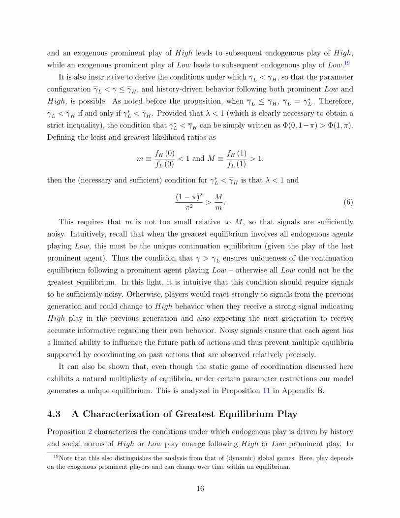
It is also instructive to derive the conditions under which γL < γH , so that the parameter

configuration γL < γ ≤ γH , and history-driven behavior following both prominent Low and

High, is possible. As noted before the proposition, when γL ≤ γH , γL = γ∗L. Therefore,

γL < γH if and only if γ∗L < γH . Provided that λ < 1 (which is clearly necessary to obtain a

strict inequality), the condition that γ∗L < γH can be simply written as Φ(0, 1−π) > Φ(1, π).

Defining the least and greatest likelihood ratios as

m ≡ fH (0)

fL (0)< 1 and M ≡ fH (1)

fL (1)> 1.

then the (necessary and sufficient) condition for γ∗L < γH is that λ < 1 and

(1− π)2

π2>

M

m. (6)

This requires that m is not too small relative to M , so that signals are sufficiently

noisy. Intuitively, recall that when the greatest equilibrium involves all endogenous agents

playing Low, this must be the unique continuation equilibrium (given the play of the last

prominent agent). Thus the condition that γ > γL ensures uniqueness of the continuation

equilibrium following a prominent agent playing Low – otherwise all Low could not be the

greatest equilibrium. In this light, it is intuitive that this condition should require signals

to be sufficiently noisy. Otherwise, players would react strongly to signals from the previous

generation and could change to High behavior when they receive a strong signal indicating

High play in the previous generation and also expecting the next generation to receive

accurate informative regarding their own behavior. Noisy signals ensure that each agent has

a limited ability to influence the future path of actions and thus prevent multiple equilibria

supported by coordinating on past actions that are observed relatively precisely.

It can also be shown that, even though the static game of coordination discussed here

exhibits a natural multiplicity of equilibria, under certain parameter restrictions our model

generates a unique equilibrium. This is analyzed in Proposition 11 in Appendix B.

4.3 A Characterization of Greatest Equilibrium Play

Proposition 2 characterizes the conditions under which endogenous play is driven by history

and social norms of High or Low play emerge following High or Low prominent play. In

19Note that this also distinguishes the analysis from that of (dynamic) global games. Here, play dependson the exogenous prominent players and can change over time within an equilibrium.

16

the next proposition, we show that when γ > γH , endogenous agents will play Low following

some signals even if the last prominent play is High—thus following a prominent play of

High, there will be a distribution of actions by endogenous agents rather than a social norm

of High. In the process, we will provide a more complete characterization of play in the

greatest equilibrium.

Let us define two more thresholds. The first one is the level of γ below which all en-

dogenous agents will play High in all circumstances, provided other endogenous agents do

the same. In particular, if a regular agent is willing to play High following a prominent

agent who played Low, then all endogenous agents are willing to play High in all periods.

A regular agent is willing to play High following a prominent agent who played Low – pre-

suming all future endogenous agents will play High – if and only if γ ≤ λ(1 − π). The

second threshold, γH , is such that above it all endogenous agents play Low, even following

prominent High. This threshold is upper bounded by (1− λ)+λ (1− π), the level of γ above

which no endogenous agent would ever play High, even if he follows a prominent agent who

has chosen High and expected all future endogenous players to play High.

Figure 2 depicts these thresholds and shows the corresponding equilibrium behavior. In

particular, it highlights that between γH and γH and between λ (1− π) and γL, behavior

immediately following a prominent agent is the same as the action of the prominent agent,

but will deviate from this thereafter. The exact pattern of behavior in these regions is

characterized in the next section. Proposition 3 summarizes the pattern shown in Figure 2.

The proposition is stated verbally here, and in the appendix we also include the state-

ments in terms of the strategy notation.

Proposition 3 In the greatest equilibrium:

1. All endogenous agents play High either if γ ≤ λ(1−π) (regardless of the last prominent

play), or if λ(1− π) < γ ≤ γH and the last prominent play was High.

2. All endogenous agents play Low either if γH < γ (regardless of the last prominent

play), or if γL < γ ≤ γH and the last prominent play was Low.

3. In the remaining regions, the play of endogenous players changes over time:

F If the last prominent play was High and γH < γ ≤ γH , then an endogenous promi-

nent player who immediately follows the last prominent play will play High, but some

other endogenous players eventually play Low for at least some signals.

17

F If the last prominent play was Low and λ(1− π) < γ ≤ γL, then a non-prominent

player who immediately follows the last prominent play will play Low, but some other

endogenous players eventually play High for at least some signals.

5 The Reversion of Play over Time

As noted in the previous section, outside of the parameter regions discussed in Proposition

2, there is an interesting phenomenon regarding the reversion of the play of regular players—

deterioration of High play starting from a prominent play of High. This is a consequence of

a more general monotonicity result, which shows that cutoffs always move in the same direc-

tion, that is, either they are monotonically non-increasing or monotonically non-decreasing,

so that High play either becomes monotonically more likely or monotonically less likely.

As a consequence, when greatest equilibrium behavior is not completely driven by the most

recent prominent play (as specified in Proposition 2), then High and Low play deteriorate

over time, meaning that as the distance from the last prominent High (resp., Low) agent

increases, the likelihood of High (resp., Low) behavior decreases and corresponding cutoffs

increase (resp., decrease).

Since we are focusing on semi-Markovian equilibria, with a slight abuse of notation,

let us denote the cutoffs used by prominent and non-prominent agents τ periods after the

last prominent agent by cPτ and cN

τ respectively. We say that High play is non-increasing

over time if (cPτ , cN

τ ) ≤ (cPτ+1, c

Nτ+1) for each τ . We say that High play is decreasing over

time, if, in addition, we have that when (cPτ , cN

τ ) 6= (0, 0) and (cPτ , cN

τ ) 6= (1, 1), (cPτ , cN

τ ) 6=(cP

τ+1, cNτ+1). The concepts of High play being non-decreasing and increasing over time are

defined analogously.

The definition of decreasing or increasing play implies that when the cutoffs for endoge-

nous agents are non-degenerate, they must actually strictly increase over time – so unless

High play completely dominates, then High play strictly decreases over time. In particular,

when γ /∈ (γL, γH ], as we know from Proposition 3, there are no constant equilibria, so High

play must be increasing or decreasing.

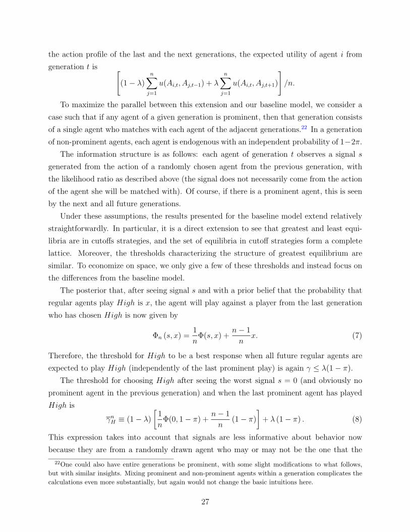
Proposition 4 1. In the greatest equilibrium, cutoff sequences(cPτ , cN

τ

)are monotone.

Thus, following a prominent agent choosing High,(cPτ , cN

τ

)are non-decreasing and

following a prominent agent choosing Low, they are non-increasing.

2. If γH < γ < γH , then in the greatest equilibrium, High play is decreasing over time

following High play by a prominent agent.

18

3. If λ(1 − π) < γ < γL, then in the greatest equilibrium, High play is increasing over

time following Low play by a prominent agent.

There is one interesting difference between the ways in which reversion occurs when it

happens from Low versus High play. Endogenous prominent agents are always at least

weakly more willing to play High than are regular agents, since they will be observed and

are thus more likely to have their High play reciprocated by the next agent. Thus, their cut-

offs are always weakly lower and their corresponding probability of playing High is higher.

Hence, if play starts at High, then it is the regular agents who are reverting more, i.e.,

playing Low with a greater probability. In contrast, if play starts at Low, then it is the

prominent agents who revert more, i.e., playing High with a greater probability (and even-

tually leading to a new prominent history beginning with a High play). It is possible, for

some parameter values, that one type of endogenous player sticks with the play of the last

prominent agent (prominent endogenous when starting with High, and non-prominent en-

dogenous when starting with Low), while the other type of endogenous player strictly reverts

in play.20

Figure 3 illustrates the behavior of the cutoffs and the corresponding probabilities of

High play for regular agents following a High prominent play. For the reasons explained in

the paragraph preceding Proposition 4, prominent endogenous agents will have lower cutoffs

and higher probabilities of High play than regular agents. Depending on the specific level

of γ, it could be that prominent endogenous agents all play High for all signals and times,

or it could be that their play reverts too.

The intuition for Proposition 4 is interesting. Immediately following a High prominent

action, an agent knows for sure that she is facing High in the previous generation. Two

periods after a High prominent action, she is playing against an agent from the previous

period who knew for sure that he was facing High in the previous generation. Thus her

opponent was likely to have chosen High himself. Nevertheless, there is the possibility that

this opponent might have been an exogenous type committed to Low, and since γ > γH , there

are some signals for which she will conclude that this opponent is indeed such an exogenous

type and choose Low instead. Now consider an agent three periods after a High prominent

action. For this agent, not only is there the possibility that one of the two previous agents

were exogenous and committed to Low play, but also the possibility that his immediate

predecessor received an adverse signal and decided to play Low instead. Thus he is even

20Note that the asymmetry between reversion starting from Low versus High play we are emphasizinghere is distinct and independent from the asymmetry that results from our focus on the greatest equilibrium.In particular, this asymmetry is present even if we focus on the least equilibrium.

19

t=0 1 2 3

x1x2

High1

Regular Agents

x3Probability High

Cutoffs

4

x4

Steady State Prob High

Steady State Cutoff

Figure 3: Reversion of Play from High to the highest Steady-State

more likely to interpret adverse signals as coming from Low play than was his predecessor.

This reasoning highlights the tendency towards higher cutoffs and less High play over time.

In fact, there is another more subtle force pushing in the same direction. Since γ > γH , each

agent also realizes that even when she chooses High, the agent in the next generation may

receive an adverse signal, and the farther this agent is from the initial prominent agent, the

more likely are the signals resulting from her choice of High to be interpreted as coming from

a Low agent. This anticipation of how her signal will be interpreted – and thus becomes more

likely to be countered by a play of Low – as the distance to the prominent agent increases

creates an additional force towards reversion.

The converse of this intuition explains why there is improvement of High play over

time starting with a prominent agent choosing Low. The likelihood of a given individual

encountering High play in the previous generation increases as the distance to prominent

agent increases as Figure 3 shows.

Proposition 4 also implies that behavior converges to a limiting (steady-state) distribution

along sample paths where there are no prominent agents. Two important caveats need to

be noted, however. First, this limiting distribution need not be unique and depends on the

starting point. In particular, the limiting distribution following a prominent agent playing

Low may be different from the limiting distribution following a prominent agent playing

High. This can be seen by considering the case where γL < γ ≤ γH studied in Proposition

2, where (trivially) the limiting distribution is a function of the action of the last prominent

agent. Second, while there is convergence to a limiting distribution along sample paths

without prominent agents, there is in general no convergence to a stationary distribution

20

because of the arrival of exogenous prominent agents. In particular, provided that q > 0

(and since π > 0), the society will necessarily fluctuate between different patterns of behavior.

For example, when γL < γ ≤ γH , as already pointed out following Proposition 2, the society

will fluctuate between social norms of High and Low play as exogenous prominent agents

arrive and choose different actions (even if this happens quite rarely).

6 Prominent Agents and Leadership

In this section, we show how prominent agents can exploit their greater visibility by future

generations in order to play a leadership role and break the Low social norm to induce a

switch to High play.

6.1 Breaking the Low Social Norm

Next consider a Low social norm where all regular agents play Low.21 Suppose that at

generation t there is an endogenous prominent agent. The key question analyzed in the next

proposition is when an endogenous prominent agent would like to switch to High play in

order to change the existing social norm.

Let γL denote the threshold such that above this level, in the greatest equilibrium, all

regular players choose Low following a prominent Low. As we show in Appendix A, 0 < γL <

γL, and so this is below the threshold where all endogenous players choose Low (because, as

we explained above, prominent endogenous agents are more willing to switch to High than

regular agents).

Proposition 5 Consider the greatest equilibrium:

1. Suppose that γL ≤ γ < min {γ∗L, γH}. Suppose also that the last prominent agent has

played Low. Then there exists a cutoff c < 1 such that an endogenous prominent agent

playing at least two periods after the last prominent agent and receiving a signal s > c

will choose High and break the Low social norm (i.e., σSMτ (a = Low, s, T = P ) =

High if s > c and τ > 1).

2. Suppose that γ < min {γL, γH}. Suppose that the last prominent agent played Low.

Then there exists a sequence of decreasing cutoffs {cτ}∞τ=2 < 1 such that an endogenous

prominent agent playing τ ≥ 2 periods after the last prominent agent and receiving

21Note that the social norm in question here involves one in which all regular agents, but not necessarilyendogenous prominent agents, play Low.

21

a signal s > cτ will choose High and switch to play from the path of convergence to

steady state to a High social norm (i.e., σSMτ (a = Low, s, T = P ) = High if s > cτ

and τ ≥ 2, and cτ is decreasing in τ with cτ < c for all τ > 1).

The results in this proposition are both important and intuitive. Their importance stems

from the fact that they show how prominent agents can play a crucial leadership role in soci-

ety. In particular, the first part shows that starting with the Low social norm, a prominent

agent who receives a signal from the last generation that is not too adverse (so that there

is some positive probability that she is playing an exogenous type committed to High play)

will find it profitable to choose High, and this will switch the entire future path of play,

creating a High social norm instead. The second part shows that prominent agents can

also play a similar role starting from a situation which does not involve a Low social norm

– instead, starting with Low and reverting to a steady state distribution. In this case, the

threshold for instigating such a switch depends on how far they are from the last prominent

agent who has chosen Low.

The intuition for these results is also interesting as it clarifies how history and expectations

shape the evolution of cooperation. Prominent agents can play a leadership role because they

can exploit their impact on future expectations and their visibility by future generations in

order to change a Low social norm into a High one. In particular, when the society is stuck

in a Low social norm, regular agents do not wish to deviate from this, because they know

that the previous generation has likely chosen Low and also that even if they were to choose

High, the signal generated by this would likely be interpreted by the next generation as

coming from a Low action. For a prominent agent, the latter is not a concern, since her

action is perfectly observed by the next generation. Moreover and perhaps more importantly

from an economic point of view, her deviation from the Low social norm can influence the

expectations of all future generations, reinforcing the incentives of the next generation to

also switch their action to High.

6.2 Prominence, Expectations and Leadership

In this subsection we highlight the role of prominence in our model, emphasizing that promi-

nence is different (stronger) than simply being observed by the next generation with certainty.

In particular, the fact that prominence involves being observed by all subsequent generations

with certainty plays a central role in our results. To clarify this, we consider four scenarios.

In each scenario, for simplicity, we assume that there is a starting non-prominent agent

at time 0 who plays High with probability x0 ∈ (0, 1), where x0 is known to all agents who

22

follow, and generates a signal for the first agent in the usual way. All agents after time 1

are not prominent. In every case all agents (including time 1 agents) are endogenous with

probability (1− 2π).

Scenario 1. The agent at time 1 is not prominent and his or her action is observed with the usual

signal structure.

Scenario 2. The agent at time 1’s action is observed perfectly by the period 2 agent, but not by

future agents.

Scenario 2′. The agent at time 1 is only observed by the next agent according to a signal, but then

is subsequently perfectly observed by all agents who follow from time 3 onwards.

Scenario 3. The agent at time 1 is prominent, and all later agents are viewed with the usual signal

structure.

Clearly, as we move from Scenario 1 to Scenario 2 (or 2′) to Scenario 3, we are moving

from a non-prominent agent to a prominent one, with Scenarios 2 and 2′ being hybrids,

where the agent of generation t = 1 has greater visibility than a non-prominent agent but is

not fully prominent in terms of being observed forever after.

We focus again on the greatest equilibrium and let ck(λ, γ, fH , fL, π) denote the cutoff

signal above which the first agent (if endogenous) plays High under scenario k as a function

of the underlying setting.

Proposition 6 The cutoffs satisfy c2(·) ≥ c3(·) and c1(·) ≥ c2′(·) ≥ c3(·), and there are

settings (λ, γ, fH , fL, π) for which the inequalities are strict.

The intuition for this result is instructive. First, comparing Scenario 2 to Scenario 3, the

former has the same observability of the action by the next generation (the only remaining

generation that directly cares about the action of the agent) but not the common knowledge

that future generations will also observe this action. This means that future generations will

not necessarily coordinate on the basis of a choice of High by this agent, and this discourages

High play by the agent at date t = 2, and through this channel, it also discourages High

play by the agent at date t = 1, relative to the case in which there was full prominence.

The comparison of Scenario 2′ to Scenario 1 is perhaps more surprising. In Scenario 2′, the

agent at date t = 1 knows that her action will be seen by future agents, so if she plays High,

then this gives agent 3 extra information about the signals that agent 2 is likely to observe.

This creates strong feedback effects in turn affecting agent 1. In particular, agent 3 would

23

choose a lower cutoff for a given cutoff of agent 2 when she sees High play by agent 1. But

knowing that agent 3 is using a lower cutoff, agent 2 will also find it beneficial to use a lower

cutoff. This not only feeds back to agent 3, making her even more aggressive in playing

High, but also encourages agent 1 to play High as she knows that agent 2 is more likely

to respond with High himself. In fact, these feedback effects continue and affect all future

agents in the same manner, and in turn, the expectation that they will play High with a

higher probability further encourages High play by agents 1 and 2. Thus, one can leverage

things upwards even through delayed prominence.

Notably, a straightforward extension of the proof of Proposition 6 shows that the same

comparisons hold if we replace “time 3” in Scenarios 2 or 2′ with “time k” for any k ≥ 3.

There are two omitted comparisons: between scenarios 2 and 2′ and between scenarios

1 and 2. Both of these are ambiguous. It is clear why the comparison between scenarios 2

and 2′ is ambiguous as those information structures are not nested. The ambiguity between

scenarios 1 and 2 is more subtle, as one might have expected that c1 ≥ c2. The reason

why this is not always the case is interesting. When signals are sufficiently noisy and x0 is

sufficiently close to 1, under scenario 1 agent 2 would prefer to choose High regardless of

the signal she receives. This would in turn induce agent 1 to choose High for most signals.

When the agent 2 instead observes agent 1’s action perfectly as in scenario 2, then (provided

that λ is not too high) she will prefer to match this action, i.e., play High only when agent

1 plays High. The expectation that she will play Low in response to Low under scenario

2 then leads agents born in periods 3 and later to be more pessimistic about the likelihood

of facing High and they will thus play Low with greater probability than they would do

under scenario 1. This then naturally feeds back and affects the tradeoff facing agent 2 and

she may even prefer to play Low following High play; in response the agent born in period

1 may also choose Low. All of this ceases to be an issue if the play of the agent born at

date 1 is observed by all future generations (as in scenarios 2′ and 3), since in this case the

ambiguity about agent 2’s play disappears.

7 Comparative Statics

We now present some comparative static results that show the role of forward versus back-

ward looking behavior and the information structure on the likelihood of different types of

social norms.

We first study how changes in λ, which capture how forward-looking the agents are,

impact the likelihood of social norms involving High and Low play. Since we do not have

24

an explicit expression for γL, we focus on the impact of λ on γH and γ∗L (recall that γL = γ∗L

when γL ≤ γH).

Proposition 7 1. γH is increasing in λ; i.e., all High endogenous play following High

prominent play occurs for a larger set of parameters as agents become more forward-

looking.

2. There exists M∗ such that γ∗L is increasing [decreasing] in λ if M < M∗ [if M > M∗],

i.e., Low play as the unique equilibrium following Low prominent play occurs for a

larger set of parameters as agents become more forward-looking provided that signals

more likely under High are sufficiently distinguishing.

The first result follows because γH is the threshold for the greatest equilibrium to involve

High following a prominent agent who chooses High. A greater λ increases the importance

of coordinating with the next generation, and this enables the choice of High being sustained

by expectations of future agents choosing High.

The second part focuses on the effects of λ on γ∗L. Recall that the greatest equilibrium

involves a social norm of Low if this is the unique (continuation) equilibrium. As λ increases,

more emphasis is placed on expectations of agents’ play tomorrow relative to interpreting

past signals. Whether this makes it easier or harder to coordinate on a Low social norm

depends on how accurate the past signals are regarding potential information that might

upset the coordination – accurate signals regarding past High can upset all Low play as

an equilibrium. Thus, when past signals are sufficiently accurate, more forward looking

preferences (i.e., higher λ) make the Low social norm following Low prominent play more

likely.

The next proposition gives comparative statics with respect to the probability of the

exogenous types, π.

Proposition 8 1. γH is decreasing in π; i.e., exclusively High play following High

prominent play occurs for a smaller set of parameter values as the probability of exoge-

nous types increases.

2. For every λ there is a threshold πλ such that for π > πλ, γ∗L is decreasing in π, and

for π < πλ, γ∗L is increasing in π. Moreover, πλ is decreasing in λ.

The results in this proposition are again intuitive. A higher π implies that there is a

higher likelihood of an exogenous type committed to Low and this makes it more difficult

to maintain the greatest equilibrium with all endogenous agents playing High (following a

25

prominent agent who has chosen High). For the second part, recall that we are trying to

maintain an equilibrium in which all endogenous agents playing Low following a prominent

Low is the unique equilibrium. A lower probability of types exogenously committed to High

makes this more likely provided that agents put sufficient weight on the past, so that the

main threat to a Low social norm comes from signals indicating that the previous generation

has played High (and this is captured by the condition that π > πλ, where πλ is decreasing

in λ). Otherwise (i.e., if π < πλ) the unique equilibrium requires all agents choosing Low

in order to target payoffs from (Low,Low) when they are matched with an exogenous type

committed to Low in the next generation. Naturally in this case a higher π makes this more

likely.

The next proposition summarizes some implications of the signals structure becoming

more informative. Comparing two information settings (fL, fH) and (fL, fH), we say that

signals become more informative if there exists s ∈ (0, 1) withbfH(s)bfL(s)

> fH(s)fL(s)

for all s > s andbfH(s)bfL(s)< fH(s)

fL(s)for all s < s.

Proposition 9 Suppose that signals become more informative from (fL, fH) to (fL, fH),

and consider a case such that γL ≤ γ < min {γ∗L, γH} both before and after the change in

the distribution of signals. If 1 > c > s (where c is the original threshold as defined in

Proposition 5), then the likelihood that a prominent agent will break a Low social norm (play

High if the last prominent play was Low) increases in the greatest equilibrium.

Prominent agents break the Low social norm when they believe that there is a sufficient

probability that the agent in the previous generation chose High (and anticipating that they

can switch the play to High given their visibility). The proposition follows because when

signals become more precise near the threshold s where prominent agents are indifferent

between sticking with and breaking the Low social norm, the probability that they will

obtain a signal greater than s increases. This increases the likelihood that they would prefer

to break the Low social norm.

8 Extensions

8.1 Multiple Agents within Generations

Suppose that there are n agents within each generation. If there are no prominent agents

in the previous and the next generations, each agent is randomly matched with one of the

n agents from the previous and one of the n agents from the next generation, so given

26

the action profile of the last and the next generations, the expected utility of agent i from

generation t is [(1− λ)

n∑j=1

u(Ai,t, Aj,t−1) + λ

n∑j=1

u(Ai,t, Aj,t+1)

]/n.

To maximize the parallel between this extension and our baseline model, we consider a

case such that if any agent of a given generation is prominent, then that generation consists

of a single agent who matches with each agent of the adjacent generations.22 In a generation

of non-prominent agents, each agent is endogenous with an independent probability of 1−2π.

The information structure is as follows: each agent of generation t observes a signal s

generated from the action of a randomly chosen agent from the previous generation, with

the likelihood ratio as described above (the signal does not necessarily come from the action

of the agent she will be matched with). Of course, if there is a prominent agent, this is seen

by the next and all future generations.

Under these assumptions, the results presented for the baseline model extend relatively

straightforwardly. In particular, it is a direct extension to see that greatest and least equi-

libria are in cutoffs strategies, and the set of equilibria in cutoff strategies form a complete

lattice. Moreover, the thresholds characterizing the structure of greatest equilibrium are

similar. To economize on space, we only give a few of these thresholds and instead focus on

the differences from the baseline model.

The posterior that, after seeing signal s and with a prior belief that the probability that

regular agents play High is x, the agent will play against a player from the last generation

who has chosen High is now given by

Φn (s, x) =1

nΦ(s, x) +

n− 1

nx. (7)

Therefore, the threshold for High to be a best response when all future regular agents are

expected to play High (independently of the last prominent play) is again γ ≤ λ(1− π).

The threshold for choosing High after seeing the worst signal s = 0 (and obviously no

prominent agent in the previous generation) and when the last prominent agent has played

High is

γnH ≡ (1− λ)

[1

nΦ(0, 1− π) +

n− 1

n(1− π)

]+ λ (1− π) . (8)

This expression takes into account that signals are less informative about behavior now

because they are from a randomly drawn agent who may or may not be the one that the

22One could also have entire generations be prominent, with some slight modifications to what follows,but with similar insights. Mixing prominent and non-prominent agents within a generation complicates thecalculations even more substantially, but again would not change the basic intuitions here.

27

current player will be matched with. Clearly, γnH is increasing in n, which implies that the

set of parameters under which High play will follow High prominent play is greater when

there are more players within each generation. This is because the signal each one receives

becomes less informative about the action that the player they will be matched with is likely

to have taken, and thus they put less weight on the signal and more weight on the action of

the last prominent agent.

This reasoning enables us to establish an immediate generalizations of Proposition 3,

with the only difference that γnH , and similarly γn

L and γnH , replace γH ,γL and γH . The most

interesting result here concerns the behavior of γnH and γn

L, which is summarized in the next

proposition.

Proposition 10 In the model with n agents within each generation, there exist greatest and

least equilibria. In the greatest equilibrium: following a prominent play of Low, there is a

Low social norm and all endogenous agents play Low (i.e., σSMτ (a = Low, s, T ) = Low for

all s, T and all τ > 0) if and only if γnL < γ. Following a prominent play of High, there is a

High social norm and all endogenous agents play High (i.e., σSMτ (a = High, s, T ) = High

for all s, T and all τ > 0) if and only if γ ≤ γnH .

The threshold γnH is increasing in n. If, in addition, γn

H ≥ γnL (which is satisfied when (6)

holds), the threshold γnL is also nonincreasing in n, so that both High and Low social norms

following, respectively, High and Low prominent play, emerge for a larger set of parameter

values. The same result also holds (i.e., the threshold γnL is nonincreasing in n) when q = 0

so that there are no prominent agents after the initial period.

The intuition for this result is related to the reason why γnH is increasing in n discussed

above. A similar reasoning also affects γnL because again more agents within a generation,

i.e., greater n, implies that the signal that each agent receives is less informative about the

action of the individual they will be matched with from the previous generation. In addition,

when there are more agents within a generation, the signal that an agent will transmit to

the next generation by choosing High is less precise (because the probability that the agent

they match with will have seen their signal is 1/n).23

23This second effect is present in general, but does not impact the thresholds γnH and γn

L, because whenthese thresholds apply, next period play is fixed (either High or Low by all endogenous agents). This effect,however, impacts other cutoffs.

Based on this effect and the lesser informativeness of signals received from the past, one might conjecturea stronger result than Proposition 10, that all cutoffs following High will be lower and all cutoffs followingLow will be higher, thus increasing the power of history in all equilibria, not just those that are completelyhistory-driven. However, this stronger conjecture turns out not to be correct because of a countervailing

28

8.2 Imperfect Prominence

As we have emphasized, prominent agents are different from non-prominent agents on two

dimensions: first, their actions are observed perfectly rather than with noise; and second,

their actions are observed by all future generations not just the next generation. Proposition

6 unpacked some distinct implications of these two differences. A natural, complementary

question is whether our results on history-driven behavior hinge on perfect observation.

To investigate this question, consider a variation where all future generations observe

the same imperfect signal concerning the action of past prominent agents. In particular,

suppose that they all receive a public signal rt ∈ {Low,High} (in addition to the private

signal st from the non-prominent agent in the previous generation) concerning the action of

the prominent agent of time t (if there is indeed a prominent agent at time t). We assume

that rt = at with probability η, where at ∈ {Low,High} is the action of the prominent

agent. Clearly, as η → 1, this environment converges to our baseline environment.

An important observation in this case is that the third part of Proposition 1 no longer

applies and the greatest and least equilibria are not necessarily semi-Markovian. This is

because, given imperfect signals about the actions of prominent agents, the play of previous

prominent agents is relevant for beliefs about the play of the last prominent agent. Nev-

ertheless, when η is sufficiently large but still strictly less than 1, the greatest equilibrium

is again semi-Markovian and is driven by history; i.e., the common signal generated by the

action of the last prominent agent. In particular, it can be shown that following a signal of

r = H, the probability that a prominent agent has indeed played High cannot be lower than

η′ ≡ πη

πη + (1− π) (1− η).

This follows because there is always a probability π that the prominent agent in question

was exogenously committed to High. For η close enough to 1, η′ is strictly greater than

Φ (0, 1− π). In that case, whenever γ ≤ γH , where γH is given by (4), the reasoning that

established Proposition 2 implies that the greatest equilibrium involves all endogenous agents

playing High (regardless of their signal) when the signal from the last prominent agent is that

she played High. A similar analysis also leads to the conclusion that when η is sufficiently

large, all endogenous agents playing Low following a prominent signal of Low is the greatest

equilibrium whenever γ > γL. Notably, for these conclusions, η needs to be greater than a

certain threshold that is strictly less than 1, and thus history-driven behavior emerges even

force: when there are more agents within a generation, the signals transmitted to the next generation areless informative and this will tend to reduce the probability that agents in the next generation will chooseHigh conditional on High by the agent in question (i.e., φτ

τ+1).

29

with signals bounded away from being fully precise.

8.3 Implications of a Public Amnesty

Part of the reason that a society gets stuck in Low play is that agents are forced to pick

actions for two periods and so the incentives to match past actions can drag their play down.

If they could adjust to play different actions against different generations, they may prefer to

switch to High in the second period of their lives and thus break out of Low play. Obvious

reasons that agents will have “sticky” play relate to various costs of changing actions. Those

could be investment costs in choosing High (“becoming educated”) or sunk costs of playing

Low (taking a corrupt or criminal action could lead to possible legal penalties). We now

show briefly that in such a situation it may be beneficial to “induce” a switch from Low

play to High by subsidizing future High play by an agent (and to let it be known that this

was subsidized). Naturally, this could be done directly by providing subsidies to High play

when this is observable. But also more interestingly, in a situation in which sunk costs of

playing Low include potential penalties, it can be achieved by forgiving the penalty from

past Low play, which can be viewed as an amnesty, i.e., a period in which an agent is allowed

to change strategies from Low to High at no cost.24

To clarify these ideas, let us briefly consider the following variation on the model. Suppose

that underlying payoffs in each interaction are similar to those in a prisoners’ dilemma:

High Low

High β, β −α, κ

Low κ,−α κ, κ

In particular, Low now has a positive payoff regardless of what the other player does. How-

ever, playing Low involves a(n expected) cost C > 0. In particular, we suppose that Low

involves corrupt or criminal behavior, and an agent who has made this choice can get caught

and punished, so that C is the expected cost of punishment. In addition, we assume that

the cost that the individual will incur from choosing Low in both periods is the same as

choosing Low only in the first period of her life, because she can get caught due to her past

Low action even if she switches to High because of her first period behavior and in this case

she will receive the same punishment.

Under these conditions, if κ > β, it becomes a dominant strategy to play Low in the

second period after having played Low in the first period of one’s life. It may even be that

a player will switch from High to Low in the second period for some ranges of beliefs and

24Tirole (1996) also discusses the implications of an amnesty.

30

costs. Focusing on the case where κ > β, the choices in this game are similar to those in

the baseline model except with one enrichment. The only strategies that could ever be part

of a best response are to choose Low in both periods, to choose High in both periods, or

play High and then Low. However, if the government legislates an amnesty for a specific

generation, whereby agents of that generation who have chosen Low in the past will not be

punished and only those who choose Low in the second period of their lives will receive the

punishment (if caught). Such an amnesty may then encourage a switch from Low to High

and can change the equilibrium social norm.

9 Conclusion

In this paper, we studied the emergence and evolution of the social norm of “cooperation”.

In our baseline model, each agent lives for two periods and interacts with agents from the

previous and next generations via a coordination game. If coordination occurs on High

play, both agents receive higher payoffs. Nevertheless, Low is a best response if an agent

expects those in the previous and the next generations to have chosen Low. Thus, society

may coordinate either on a payoff-dominant (High, High) or less attractive (Low,Low)

equilibrium, leading to a High or Low social norm, whereby High (or Low) actions persist,

and are expected to persist, for a long time.

Social norms defined as “frames of reference,” shape how information from the past

is interpreted – because agents only receive noisy information about past play. History –

shared, common knowledge past events – anchors these social norms. For example, if history

indicates that there is a Low social norm (e.g., due to a Low prominent play which can then

lock-in regular players to uniquely Low play), then even moderately favorable signals of past

actions will be interpreted as due to noise and agents would be unwilling to switch to High.

This leads to a form of history-driven social norm, potentially persisting for a long time. The

role of social norms as frames of reference is central: Low behavior persists partly because,

given the social norm, the signals the agents would generate even with a High action would

be interpreted as if they were coming from a Low action, and this discourages High actions.

The impact of history is potentially countered by “prominent” agents, whose actions are

more visible. In particular, actions by prominent agents are observed by all future agents

and this creates the possibility that future generations will coordinate on the action of a

prominent agent. Even when history drives behavior, social norms will not be everlasting,

because prominent agents exogenously committed to one or the other mode of behavior may

arrive and cause a switch in play – and thus in the resulting social norm. More interestingly,

31

prominent agents can also endogenously leverage their greater visibility and play a leadership

role by coordinating the expectations of future generations. In this case, starting from a Low

social norm, a prominent agent may choose to break the social norm and induce a switch to

a High social norm in society.

We also showed that in equilibria that are not completely driven by history, there is a

pattern of “reversion” whereby play starting with High (Low) reverts toward lower (higher)

cooperation. The reason for this is interesting: an agent immediately following a prominent

High knows that she is playing against a High action in the past. An agent two periods

after a prominent High, on the other hand, must take into account that there may have

been an exogenous non-prominent agent committed to Low in the previous period. Three

periods after a prominent High, the likelihood of an intervening exogenous non-prominent

agent committed to Low is even higher. But more importantly, there are two additional

forces pushing towards reversion: first, these agents will anticipate that even endogenous

non-prominent agents now may start choosing Low because they are unsure of who they

are playing in the previous generation and an adverse signal will make them believe that

they are playing an exogenous non-prominent agent committed to Low, encouraging them to

also do Low; and second, they will also understand that the signals that their High action

will generate may also be interpreted as if they were coming from a Low action, further

discouraging High.

Several areas of future work based on our approach, and more generally based on the

interplay between history, social norms and interpretation of past actions, appear promising.

First, our analysis can be extended to the case where the stage game is not a coordination

game. For example, similar sorts of reasoning will apply when this game takes the form

of a prisoner’s dilemma and would enable a study of how cooperation in the prisoner’s

dilemma is affected by interpretation of information and signaling motives of agents taking

this into account. Relatedly, it would be useful to extend the analysis of the role of history,

expectations and leadership to a model of collective action, in which individuals care about

how many people, from the past and future generations, will take part in some collective

action, such as an uprising or demonstration against a regime.

Second, it is important to endogenize prominence in the setup, so that individuals can,

at a cost, become prominent and change the social norm. Though this introduces some

complications (e.g., because such a game is no longer one of strategic complements), several of

the general insights presented here should continue to apply in such an extended framework.

Third and relatedly, in some situations non-prominent agents in our model have an

incentive to communicate their behavior, since by doing so they can avoid the need to rely on

32

social norms for forming accurate expectations of past and future play. Another interesting

future direction is to study the evolution of social norms in situations where incentives are

not fully aligned, so that communication does not fully circumvent the role of social norms

in coordinating expectations.

Finally, it is important to introduce an explicit network structure in the pattern of obser-

vation and interaction so that agents who occupy a central position in the social network –

whose actions are thus known to be more likely to be observed by many others in the future

– (endogenously) play the role of prominent agents in our baseline model. This will help us

get closer to understanding which types of agents, and under which circumstances, can play

a leadership role.

References

[1] Anderlini, L., Gerardi, D., and Lagunoff, R. A “Super” Folk Theorem for

dynastic repeated games. Economic Theory 37, 3 (2008), 357–394.

[2] Argenziano, R., and Gilboa, I. History as a coordination device. Mimeo, 2010.

[3] Banfield, E. The Moral Basis of a Backward Society. Free Press, New York, 1958.

[4] Bisin, A., and Verdier, T. The economics of cultural transmission and the dynamics

of preferences. Journal of Economic Theory 97, 2 (2001), 298–319.

[5] Carlsson, H., and van Damme, E. Global games and equilibrium selection. Econo-

metrica 61, 5 (1993), 989–1018.

[6] Chamley, C. Coordinating regime switches. Quarterly Journal of Economics, 114, 3

(1999), 869-905.

[7] Chassang, S. Building Routines: Learning, Cooperation, and the Dynamics of In-

complete Relational Contracts American Economic Review 100, 1 (2010), 448 – 465

[8] Corsetti, G., Dasgupta, A., Morris, S., and Shin, H. S. Does one Soros make a

difference? A theory of currency crises with large and small traders. Review of Economic

Studies 71, 1 (2004), 87–113.

[9] Diamond, P. and D. Fudenberg Rational expectations business cycles in search

equilibrium. Journal of Political Economy, 97, 3 (1989), 606 – 619.

33

[10] Doepke, M., and Zilibotti, F. Occupational choice and the spirit of capitalism.

Quarterly Journal of Economics 123, 2 (2008), 747–793.

[11] Ellison, G. Learning from personal experience: one rational guy and the justification

of myopia. Games and Economic Behavior, 19, 2, (1997), 180 – 210.

[12] Frankel, D. M., and Pauzner, A. Resolving indeterminacy in dynamic settings:

The role of shocks. Quarterly Journal of Economics 115, 1 (2000), 285–304.

[13] Fudenberg, D., and Levine, D. K. The Theory of Learning in Games. MIT Press,

1998.

[14] Galor, O. Unified Growth Theory. Princeton University Press, 2011.

[15] Hermalin, B. E. Leadership and corporate culture, forthcoming in R. Gibbons and

J. Roberts (editors) Handbook of Organizations, Princeton University Press, 2012.

[16] Jackson, M. O., and Peck, J. Speculation and Price Fluctuations with Private,

Extrinsic Signals. Journal of Economic Theory, (1991), 55, 274-295.

[17] Jackson, M. O., and Yariv, L. Diffusion of behavior and equilibrium properties in

network games. American Economic Review 97, 2 (2007), 92–98.

[18] Kandori, M., Mailath, G. J., and Rob, R. Learning, mutation, and long run

equilibria in games. Econometrica 61, 1 (1993), 29–56.

[19] Kleinberg, J. Cascading behavior in networks: Algorithmic and economic issues. in

Algorithmic game theory. Cambridge University Press, 2007, 613–632.

[20] Krugman, P. History versus expectations. Quarterly Journal of Economics 106, 2

(1991), 651–667.

[21] Lagunoff, R., and Matsui, A. Asynchronous choice in repeated coordination

games. Econometrica 65, 6 (1997), 1467–1477.

[22] Locke, R. M. Building trust. in A. Flora (editor) Mezzogiorno e Politiche di Sviluppo,

Naples: Edizioni Scientifiche Italiane: 109-133.

[23] Mailath, G. J., and Samuelson, L. Repeated Games and Reputations. Oxford

University Press, 2006.

34

[24] Matsuyama, K. Increasing returns, industrialization, and indeterminacy of equilib-

rium. Quarterly Journal of Economics 106, 2 (1991), 617–650.

[25] Milgrom, P., and Shannon, C. Monotone comparative statics. Econometrica 62,

1 (1994), 157–180.

[26] Morris, S. Contagion. Review of Economic Studies 67, 1 (2000), 57–78.

[27] Morris, S., and Shin, H. S. Unique equilibrium in a model of self-fulfilling currency

attacks. American Economic Review 88, 3 (1998), 587–597.

[28] Myerson, R. Towards a theory of leadership and state-building. Mimeo. University

of Chicago, 2011.

[29] Putnam, R. D. Making Democracy Work. Princeton University Press, 1993.

[30] Sabetti, F. Path dependency and civic culture: some lessons from Italy about inter-

preting social experiments. Politics and Society, 24, 1 (1996), 19-44.

[31] Samuelson, L. Evolutionary Games and Equilibrium Selection. MIT Press, 1997.

[32] Steiner, J., and Stewart, C. Contagion through learning. Theoretical Economics

3, 4 (2008), 431–458.

[33] Straccia, U., Ojeda-Aciego, M., and Damasio, C. V. On fixed-points of multi-

valued functions on complete lattices and their application to generalized logic programs.

SIAM Journal on Computing 38, 5 (2009), 1881–1911.

[34] Tabellini, G. The scope of cooperation: Values and incentives. Quarterly Journal of

Economics 123, 3 (2008), 905–950.

[35] Tarski, A. A lattice-theoretical fixpoint theorem and its applications. Pacific Journal

of Mathematics 5, 2 (1955), 285–309.

[36] Tirole, J. A theory of collective repetitions (with applications to the persistence of

corruption in the firm quality). Review of Economic Studies, 63, 1 (1996), 1-22.

[37] Topkis, D. M. Equilibrium points in nonzero-sum n-person submodular games. SIAM

Journal on Control and Optimization 17, 6 (1979), 773–787.

[38] Van Zandt, T., and Vives, X. Monotone equilibria in Bayesian games of strategic

complementarities. Journal of Economic Theory 134, 1 (2007), 339–360.

35

[39] Vives, X. Nash equilibrium with strategic complementarities. Journal of Mathematical

Economics 19, 3 (1990), 305–321.

[40] Young, H. P. The evolution of conventions. Econometrica 61, 1 (1993), 57–84.

[41] Zhou, L. The set of Nash equilibria of a supermodular game is a complete lattice.

Games and Economic Behavior 7, 2 (1994), 295–300.

Appendix A

Equilibrium Definition

Our definition of equilibrium is standard and requires that agents best respond to their

beliefs conditional on any history and signal and given the strategies of others.25 The only

thing that we need to be careful about is defining those beliefs. In cases where 0 < q < 1

and π > 0 those beliefs are easily derived from Bayes’ rule (and an appropriate iterative

application of (2)). We provide a careful definition that also allows for q = 0 or π = 0 even

though in the text we have assumed q > 0 and π > 0. Essentially, in these corner cases

some additional care is necessary since some histories off the equilibrium path may not be

reached.26

Consider any t ≥ 1, any history ht−1, and a strategy profile σ.

Let φtt+1(σt+1, Tt, h

t−1) be the probability that, given strategy σt+1, the next agent will

play High if agent t plays High and is of prominence type Tt ∈ {P, N}. Note that this is

well-defined and is independent of the signal that agent t observes.

Let φtt−1(σ, st, h

t−1) denote the probability that agent t assigns to the previous agent

playing High given signal st, strategy profile σ, and history ht−1. In particular: if ht−1 =

High then set φtt−1(σ, st, h

t−1) = 1 and if ht−1 = Low then set φtt−1(σ, st, h

t−1) = 0. If

ht−1 = N then define φtt−1(σ, st, h

t−1) via an iterative application Bayes’ rule. Specifically,

this is done via an application of (2) as follows. Let τ be the largest element of {1, . . . , t−1}25Definitions for perfect Bayesian equilibrium and sequential equilibrium are messy when working with

continua of private signals, and so it is easiest to provide a direct definition of equilibrium here which isrelatively straightforward.

26These beliefs can still be consequential. To see an example of why this matters in our context, considera case where all agents are endogenous and prominent (so π = 0 and q = 1, which is effectively a completeinformation game). Let an agent be indifferent between High and Low if both surrounding generationsplay Low, but otherwise strictly prefer High. Begin with agent 0 playing Low. There is a (Bayesian) Nashequilibrium where all agents play Low regardless of what others do, but it is not perfect (Bayesian). Thisleads to different minimal equilibria depending on whether one works with Bayesian or perfect Bayesianequilibrium.

36

such that hτ 6= N , so the date of the last prominent agent. Then given στ+1(hτ , N, sτ+1) and

π, there is an induced distribution on High and Low by generation τ +1 and thus over sτ+2

(and note that sτ+1 is irrelevant since τ is prominent). Then given στ+2(hτ , N, sτ+2) and π,

there is an induced distribution on High and Low by generation τ + 2, and so forth. By

induction, there is an induced distribution on High and Low at time t − 1, which we then

denote by xt−1. Then φtt−1(σ, st, h

t−1) = Φ(st, xt−1) where Φ is defined in (2).

From (3), it is a best response for agent t to play High if

(1− λ) φtt−1(σ, st, h

t−1) + λφtt+1(σt+1, Tt, h

t−1) > γ, (9)

to play Low if

(1− λ) φtt−1(σ, st, h

t−1) + λφtt+1(σt+1, Tt, h

t−1) < γ, (10)

and either if there is equality.

We say that σ forms an equilibrium if for each time t ≥ 1, history ht−1 ∈ Ht−1, signal

st ∈ [0, 1], and type Tt ∈ {P, N} σt(ht−1, st, Tt) = 1 if (9) holds and σt(h

t−1, st, Tt) = 0 if

(10) holds, where φtt−1(σ, st, h

t−1) and φtt+1(σt+1, Tt, h

t−1) are as defined above.

Equilibria in Games with Strategic Complementarities and Infinitely

Many Agents

We now establish a theorem that will be used in proving Proposition 1. This theorem is

also of potential independent interest for this class of overlapping-generation incomplete

information games.

Well-known results for games of strategic complements apply to finite numbers of agents

(e.g., see Topkis (1979), Vives (1990), Milgrom and Shannon (1994), Zhou (1994), and van

Zandt and Vives (2007)). The next theorem provides an extension for arbitrary sets of

agents, including countably and uncountably infinite sets of agents.

Let us say that a game is a game of weak strategic complements with a possibly infinite

number of agents if the agents are indexed by i ∈ I and:

• each agent has an action space Ai that is a complete lattice with a partial ordering ≥i

and corresponding supi and infi;

• for every agent i, and specification of strategies of the other agents, a−i ∈ Πj 6=i,j∈IAj,

agent i has a nonempty set of best responses BRi(a−i) that is a closed sublattice of

Ai (where “closed” here is in the lattice-sense, so that sup(BRi(a−i)) ∈ BRi(a−i) and

inf(BRi(a−i)) ∈ BRi(a−i));

37

• for every agent i, if a′j ≥j aj for all j 6= i, j ∈ I, then supi BRi(a′−i) ≥i supi BRi(a−i)

and infi BRi(a′−i) ≥i infi BRi(a−i).

For the next theorem, define a ≥ a′ if and only if ai ≥i a′i for all i. The lattice of equilibria

on A = ΠAi∈I can then be defined with respect to this partial ordering.27

Theorem 1 Consider a game of weak strategic complements with a possibly infinite number

of agents. A pure strategy equilibrium exists, and the set of pure strategy equilibria form a

complete lattice.

Proof of Theorem 1: Let A = Πi∈IAi. Note that A is a complete lattice, where we say

that a ≥ a′ if and only if ai ≥ a′i for every i ∈ I, and where for any S ⊂ A we define

sup(S) = (supi{ai : a ∈ S})i∈I ,

and similarly

inf(S) = (infi{ai : a ∈ S})i∈I .

Given the lattice A, we define the best response correspondence f : A → 2A by

f(a) = (BRi{a−i})i∈I

By the definition of a game of strategic complements, BRi(a−i) is a nonempty closed sublat-

tice of Ai for each i and a−i, and so it follows directly that f(a) is a nonempty closed sublattice

of A for every a ∈ A. Note that by the strategic complementarities f is monotone: if a ≥ a′

then sup(f(a)) ≥ sup(f(a′)) and inf(f(a)) ≥ inf(f(a′)). This follows directly from the fact

that if a′−i ≥ a−i, then sup BRi(a′−i) ≥i sup BRi(a−i) (and inf BRi(a

′−i) ≥i inf BRi(a−i)) for

each i.

Thus, by an extension of Tarski’s (1955) fixed point theorem due to Straccia, Ojeda-

Aciego, and Damasio (2009) (see also Zhou (1994)),28 f has a fixed point and its fixed points

form a complete lattice (with respect to ≥). Note that a fixed point of f is necessarily a

best response to itself, and so is a pure strategy equilibrium, and all pure strategy equilibria

are fixed points of f , and so the pure strategy equilibria are exactly the fixed points of f .

27Note, however, that the set of equilibria is not necessarily a sublattice of A, as pointed out in Topkis(1979) and in Zhou (1994) for the finite case. That is, the sup in A of a set of equilibria may not be anequilibrium, and so sup and inf have to be appropriately defined over the set of equilibria to ensure that theset is a complete lattice. Nevertheless, the same partial ordering can be used to define the greatest and leastequilibria.

28The monotonicity of f here implies the EM -monotonicity in Proposition 3.15 of Straccia, Ojeda-Aciego,and Damasio (2009).

38

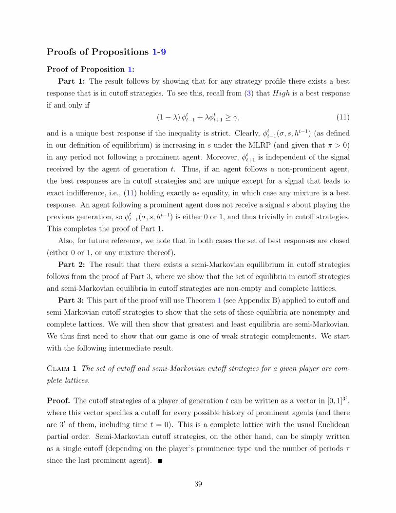
Proofs of Propositions 1-9

Proof of Proposition 1:

Part 1: The result follows by showing that for any strategy profile there exists a best

response that is in cutoff strategies. To see this, recall from (3) that High is a best response

if and only if

(1− λ) φtt−1 + λφt

t+1 ≥ γ, (11)

and is a unique best response if the inequality is strict. Clearly, φtt−1(σ, s, ht−1) (as defined

in our definition of equilibrium) is increasing in s under the MLRP (and given that π > 0)

in any period not following a prominent agent. Moreover, φtt+1 is independent of the signal

received by the agent of generation t. Thus, if an agent follows a non-prominent agent,

the best responses are in cutoff strategies and are unique except for a signal that leads to

exact indifference, i.e., (11) holding exactly as equality, in which case any mixture is a best

response. An agent following a prominent agent does not receive a signal s about playing the

previous generation, so φtt−1(σ, s, ht−1) is either 0 or 1, and thus trivially in cutoff strategies.

This completes the proof of Part 1.

Also, for future reference, we note that in both cases the set of best responses are closed

(either 0 or 1, or any mixture thereof).

Part 2: The result that there exists a semi-Markovian equilibrium in cutoff strategies

follows from the proof of Part 3, where we show that the set of equilibria in cutoff strategies

and semi-Markovian equilibria in cutoff strategies are non-empty and complete lattices.

Part 3: This part of the proof will use Theorem 1 (see Appendix B) applied to cutoff and

semi-Markovian cutoff strategies to show that the sets of these equilibria are nonempty and

complete lattices. We will then show that greatest and least equilibria are semi-Markovian.

We thus first need to show that our game is one of weak strategic complements. We start

with the following intermediate result.

Claim 1 The set of cutoff and semi-Markovian cutoff strategies for a given player are com-

plete lattices.

Proof. The cutoff strategies of a player of generation t can be written as a vector in [0, 1]3t,

where this vector specifies a cutoff for every possible history of prominent agents (and there

are 3t of them, including time t = 0). This is a complete lattice with the usual Euclidean

partial order. Semi-Markovian cutoff strategies, on the other hand, can be simply written

as a single cutoff (depending on the player’s prominence type and the number of periods τ

since the last prominent agent).

39

Next, we verify the strategic complementarities for cutoff strategies. Let zt−1(σ, ht−1)

be the prior probability that this agent assigns to an agent of the previous period play-

ing High conditional on ht−1 (and before observing s). Fix a cutoff strategy profile c =(cN1 (h0) , cP

1 (h0) , ...cNt (ht−1) , cP

t (ht−1) , ...). Suppose that sup BRT

t (c) is the greatest best

response of agent of generation t of prominence type T to the cutoff strategy profile c (mean-

ing that it is the best response with the lowest cutoffs). Now consider c =(cN1 (h0) , cP

1 (h0) , ...cNt (ht−1) , cP

t (ht−1) , ...)≤

c =(cN1 (h0) , cP

1 (h0) , ...cNt (ht−1) , cP

t (ht−1) , ...). We will show that sup BRT

t (c) ≥ sup BRTt (c)

(the argument for inf BRTt (c) ≥ inf BRT

t (c) is analogous). First, cutoffs after t + 2 do not

affect BRTt (c). Second, suppose that all cutoffs before t− 1 remain fixed and cN

t+1 and cPt+1

decrease (meaning that they are weakly lower for every history and at least one of them

is strictly lower for at least one history). This increases φtt+1(σ, T, ht−1) and thus makes

(11) more likely to hold, so sup BRTt (c) ≥ sup BRT

t (c). Third, suppose that all cutoffs

before t − 2 remain fixed, and cNt−1 and cP

t−1 decrease. This increases zt−1(σ, ht−1) and thus

φtt−1(σ, s, ht−1) and thus makes (11) more likely to hold, so again sup BRT

t (c) ≥ sup BRTt (c).

Fourth, suppose that all other cutoffs remained fixed and cNt−k−1 and cP

t−k−1 (for k ≥ 1) de-

crease. By MLRP, this shifts the distribution of signals at time t−k in the sense of first-order

stochastic dominance and thus given cNt−k and cP

t−k, it increases zt−k(σ, ht−k−1), shifting the

distribution of signals at time t − k + 1 in the sense of first-order static dominance. Ap-

plying this argument iteratively k times, we conclude that sup BRTt (c) ≥ sup BRT

t (c). This

establishes that whenever c ≥ c, sup BRTt (c) ≥ sup BRT

t (c). The same argument also ap-

plies to semi-Markovian cutoffs. Thus from Theorem 1 the set of pure strategy equilibria in

cutoff strategies and set of pure strategy semi-Markovian equilibria in cutoff strategies are

nonempty complete lattices.

To complete the proof, we next show that greatest and least equilibria are semi-Markovian.

We provide the argument for the greatest equilibrium and the argument for the least is analo-

gous. It is clear that the overall greatest equilibrium is at least as high (with cutoffs at least as

low) as the greatest semi-Markov equilibrium since it includes such equilibria, so it is sufficient

to show that the greatest equilibrium is semi-Markovian. Thus, suppose to the contrary of

the claim that the greatest equilibrium, say c =(cN1 (h0) , cP

1 (h0) , ...cNt (ht−1) , cP

t (ht−1) , ...),

is not semi-Markovian. This implies that that there exists some t (and T ∈ {P, N}) such that

cTt (ht−1) > cT

t

(ht−1

)where ht−1 and ht−1 have the same last prominent agent, say occurring

at time t−k. Then consider c = (cN1 (h0) , cP

1 (h0) , ..., cNt−k+1

(ht−k

), cP

t−k+1

(ht−k

), cN

t−k+2

(ht−k+1

), cP

t−k+2

(ht−k+1

),

... cNt (ht−1) , cP

t (ht−1) , cNt+1 (ht) , cP

t+1 (ht) , ...), where cTt−k+j+1

(ht−k+j

)= min{ctt− k + j + 1T

(ht−k+j

), cT

t−k+j+1

(ht−k+j

)}

with ht−k+j and ht−k+j are the truncated versions of histories ht−1 and ht−1. Next, it is

straightforward to see that c is also an equilibrium. In particular, note that following history

40

ht−1, c is an equilibrium by hypothesis. Since the payoffs of none of the players after t − k

directly depend on the action of the prominent agents before the last one, this implies that

when all agents after t − k switch their cutoffs after history ht−k as in c, this is still an

equilibrium. This shows that c is an equilibrium cutoff profile, but this contradicts that c is

the greatest equilibrium.

Proof of Proposition 2: First, we state the proposition in terms of strategies. Let us

denote the greatest equilibrium (which is necessarily semi-Markovian) by σSMτ (a, s, T ) and

the least equilibrium by σSMτ (a, s, T ). Then the greatest equilibrium is such that:

1. following a prominent play of Low, there is a Low social norm and all endogenous

agents play Low (i.e., σSMτ (a = Low, s, T ) = Low for all s, T and all τ > 0) if and

only if γL < γ; and

2. following a prominent play of High, there is a High social norm and all endogenous

agents play High (i.e., σSMτ (a = High, s, T ) = High for all s, T and all τ > 0) if and

only if γ ≤ γH .

Thus, endogenous players always follow the play of the most recent prominent player in

the greatest equilibrium if and only if γL < γ ≤ γH .

We first prove the second part of the proposition, and then return to the first part. And

finally, we prove that if γL ≤ γH , then γL = γ∗L; thus deriving (6) as a necessary and sufficient

condition for γL < γH .

Part 2: Suppose the last prominent agent has played a = High. Let φττ−1 and φτ

τ+1 be

the expectations of an endogenous agent τ periods after the last prominent agent that the

previous and next generations will play High. Let zτ−1(σ, High) be the prior probability

that this agent assigns to an agent of the previous period playing High conditional on the

last prominent agent having played a = High. In an equilibrium where all endogenous agents

play High, it follows that zτ−1(σ, High) = 1− π (since only exogenous agents committed to

Low will not do so). Hence, the lowest possible value of φττ−1(σ, s, High) is

mins∈[0,1]

{zτ−1(σ, High)

zτ−1(σ, High) + (fL (s) /fH(s)) (1− zτ−1(σ, High))

}= Φ(0, 1− π).

Moreover, in an equilibrium where all endogenous agents play High, we also have φττ+1 =

1− π. Then provided that

(1− λ) Φ(0, 1− π) + λ (1− π) ≥ γ,

41

or equivalently, provided that γ ≤ γH , σSMτ (a = High, s, T ) = High for all s and T is a

best response. Conversely, if this condition fails, then all High is not a best response. Thus,

we have established that if γ ≤ γH , then all endogenous agents playing High following a

prominent High is an equilibrium, and otherwise, it is not an equilibrium.

Part 1: For γ sufficiently large, all endogenous players playing Low is clearly the unique

equilibrium. In particular, if γ > (1 − λ) + λ(1 − π),then even under the most optimistic

conceivable beliefs – that the last agent was certain to have played High and the next agent

will play High unless she is exogenously and committed to Low – we have σSMτ (a, s, T ) =

Low for all a, s and T . Thus, for sufficiently high (but less than one, since (1−λ)+λ(1−π) <

1) γ, all Low following a prominent Low is the unique continuation equilibrium regardless

of others actions and history (meaning that all Low following a prominent Low is part

of all equilibria). Conversely, for sufficiently low (e.g., less than λπ) but still positive γ

all endogenous agents playing High following a prominent Low is the unique equilibrium.

Next, note that the set of γ for which all endogenous agents playing Low following the last

prominent agent playing Low is the unique equilibrium is an interval. This follows directly

from (3), since if Low is a best response for some γ for all endogenous agents, then it is

also a best response for all endogenous agents for all higher γ. Now consider the interval

of γ’s for which all endogenous agents playing Low following the last prominent Low is the

unique continuation equilibrium. The above arguments establish that this interval is strictly

between 0 and 1. Define the lowest endpoint of this interval as γL. Then, by construction,

when γ > γL, the greatest equilibrium involves all endogenous agents playing Low following

a prominent Low, and when γ ≤ γL, all Low following a prominent Low is not the greatest

equilibrium.

Proof that γL ≤ γH implies γL = γ∗L. Suppose γL ≤ γH and consider the case where

γ = γL. Then following a High play of a prominent agent, all endogenous agents will play

High. Therefore, for an endogenous prominent agent to have Low as best response for any

signal and prior x, it has to be the case that (1− λ)Φ(1, x) + λ(1− π) ≤ γL. Since γL ≤ γ∗L,

this implies

(1− λ)Φ(1, x) + λ(1− π) ≤ γL ≤ (1− λ)Φ(1, π) + λ(1− π).

Therefore, Φ(1, x) ≤ Φ(1, π), or equivalently x = π as π is the lowest possible prior of pre-

vious agent playing High. Hence γL = γ∗L.

This immediately implies that when γ∗L ≤ γH , we also have γL = γ∗L. Then (6) is obtained

by comparing the expressions for γH and γ∗L.

42

Proof of Proposition 3: We include more formal descriptions of the statement of the

proposition. In the greatest equilibrium:

1. All endogenous agents play High either if γ ≤ λ(1−π) (regardless of the last prominent

play; i.e., σSMτ (a, s, T ) = High for all a, s, T and all τ > 0), or if λ(1− π) < γ ≤ γH

and the last prominent play was High (i.e., σSMτ (High, s, T ) = High for all s, T and

all τ > 0).

2. All endogenous agents play Low either if γH < γ (regardless of the last prominent

play; i.e., σSMτ (a, s, T ) = Low for all a, s, T and all τ > 0), or if γL < γ ≤ γH and the

last prominent play was Low (i.e., σSMτ (Low, s, T ) = Low for all s, T and all τ > 0).

3. In the remaining regions, the play of endogenous players changes over time:

F If the last prominent play was High and γH < γ ≤ γH , then an endogenous promi-

nent player who immediately follows the last prominent play will play High, but some

other endogenous (non-prominent, and possibly also prominent) players eventually play

Low for at least some signals (i.e., σSM1 (High, s, P ) = High and σSM

τ (a, s, T ) = Low

for some s, T and τ > 0).

F If the last prominent play was Low and λ(1− π) < γ ≤ γL, then a non-prominent

player who immediately follows the last prominent play will play Low, but some other

endogenous (prominent and possibly also non-prominent) players eventually play High

for at least some signals (i.e., σSM1 (Low, s,N) = Low and σSM

τ (a, s, T ) = High for

some s, T and τ > 0).

Part 1: Note that if a regular agent is willing to play High following a prominent Low

when other endogenous agents play High, then all endogenous agents are willing to play

High in all periods. A regular agent is willing to play High following a prominent Low

when other endogenous agents play High provided that γ ≤ λ(1− π). Thus, below this all

playing High by all endogenous agents is an equilibrium. Next, note that if γ > λ(1 − π),

then a regular agent immediately following a prominent Low will necessarily have a unique

best response of playing Low even with the most optimistic beliefs about the future, and so

above this level all playing High following a prominent Low is not an equilibrium.

Part 2: The arguments for establishing that a threshold γH , such that above this all

endogenous agents play Low, and below which some endogenous agents play High in some

circumstances, is analogous to the proof of the existence of the threshold γL in Proposition

2. In particular, the set of γ’s for which this is true is an interval strictly between 0 and 1,

and we define γH as the lowest endpoint of this interval.

43

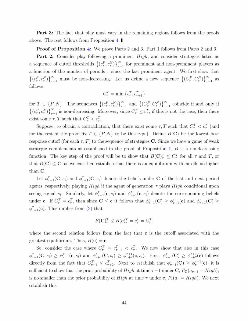
Part 3: The fact that play must vary in the remaining regions follows from the proofs

above. The rest follows from Proposition 4.

Proof of Proposition 4: We prove Parts 2 and 3. Part 1 follows from Parts 2 and 3.

Part 2: Consider play following a prominent High, and consider strategies listed as

a sequence of cutoff thresholds{(cP

τ , cNτ )

}∞τ=1

for prominent and non-prominent players as

a function of the number of periods τ since the last prominent agent. We first show that{(cP

τ , cNτ )

}∞τ=1

must be non-decreasing. Let us define a new sequence{(CP

τ , CNτ )

}∞τ=1

as

follows:

CTτ = min

{cTτ , cT

τ+1

}for T ∈ {P, N}. The sequences

{(cP

τ , cNτ )

}∞τ=1

and{(CP

τ , CNτ )

}∞τ=1

coincide if and only if{(cP

τ , cNτ )

}∞τ=1

is non-decreasing. Moreover, since CTτ ≤ cT

τ , if this is not the case, then there

exist some τ , T such that CTτ < cT

τ .

Suppose, to obtain a contradiction, that there exist some τ , T such that CTτ < cT

τ (and

for the rest of the proof fix T ∈ {P, N} to be this type). Define B(C) be the lowest best

response cutoff (for each τ , T ) to the sequence of strategies C. Since we have a game of weak

strategic complements as established in the proof of Proposition 1, B is a nondecreasing

function. The key step of the proof will be to show that B(C)Tτ ≤ CT

τ for all τ and T , or

that B(C) ≤ C, as we can then establish that there is an equilibrium with cutoffs no higher

than C.

Let φττ−1(C, si) and φτ

τ+1(C, si) denote the beliefs under C of the last and next period

agents, respectively, playing High if the agent of generation τ plays High conditional upon

seeing signal si. Similarly, let φττ−1(c, si) and φτ

τ+1(c, si) denote the corresponding beliefs

under c. If CTτ = cT

τ , then since C ≤ c it follows that φττ−1(C) ≥ φτ

τ−1(c) and φττ+1(C) ≥

φττ+1(c). This implies from (3) that

B(C)Tτ ≤ B(c)T

τ = cTτ = CT

τ ,

where the second relation follows from the fact that c is the cutoff associated with the

greatest equilibrium. Thus, B(c) = c.

So, consider the case where CTτ = cT

τ+1 < cTτ . We now show that also in this case

φττ−1(C, si) ≥ φτ+1

τ (c, si) and φττ+1(C, si) ≥ φτ+1

τ+2(c, si). First, φττ+1(C) ≥ φτ+1

τ+2(c) follows

directly from the fact that CTτ+1 ≤ cT

τ+2. Next to establish that φττ−1(C) ≥ φτ+1

τ (c), it is

sufficient to show that the prior probability of High at time τ−1 under C, PC(aτ−1 = High),

is no smaller than the prior probability of High at time τ under c, Pc(aτ = High). We next

establish this:

44

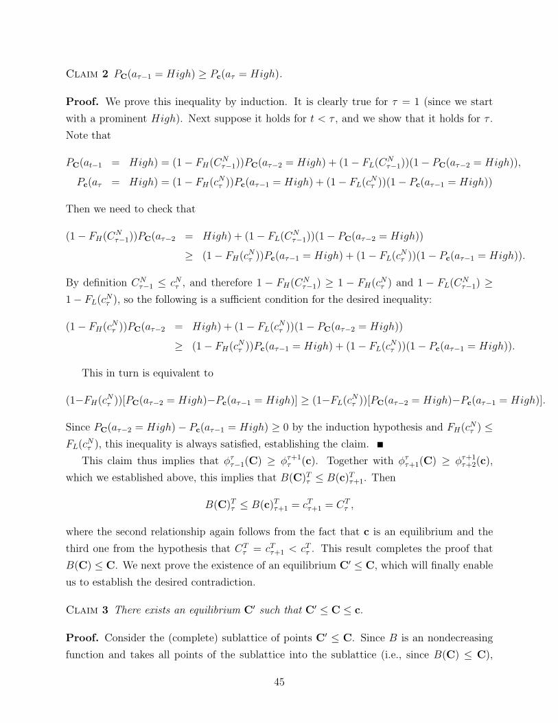
Claim 2 PC(aτ−1 = High) ≥ Pc(aτ = High).

Proof. We prove this inequality by induction. It is clearly true for τ = 1 (since we start

with a prominent High). Next suppose it holds for t < τ , and we show that it holds for τ .

Note that

PC(at−1 = High) = (1− FH(CNτ−1))PC(aτ−2 = High) + (1− FL(CN

τ−1))(1− PC(aτ−2 = High)),

Pc(aτ = High) = (1− FH(cNτ ))Pc(aτ−1 = High) + (1− FL(cN

τ ))(1− Pc(aτ−1 = High))

Then we need to check that

(1− FH(CNτ−1))PC(aτ−2 = High) + (1− FL(CN

τ−1))(1− PC(aτ−2 = High))

≥ (1− FH(cNτ ))Pc(aτ−1 = High) + (1− FL(cN

τ ))(1− Pc(aτ−1 = High)).

By definition CNτ−1 ≤ cN

τ , and therefore 1 − FH(CNτ−1) ≥ 1 − FH(cN

τ ) and 1 − FL(CNτ−1) ≥

1− FL(cNτ ), so the following is a sufficient condition for the desired inequality:

(1− FH(cNτ ))PC(aτ−2 = High) + (1− FL(cN

τ ))(1− PC(aτ−2 = High))

≥ (1− FH(cNτ ))Pc(aτ−1 = High) + (1− FL(cN

τ ))(1− Pc(aτ−1 = High)).

This in turn is equivalent to

(1−FH(cNτ ))[PC(aτ−2 = High)−Pc(aτ−1 = High)] ≥ (1−FL(cN

τ ))[PC(aτ−2 = High)−Pc(aτ−1 = High)].

Since PC(aτ−2 = High)− Pc(aτ−1 = High) ≥ 0 by the induction hypothesis and FH(cNτ ) ≤

FL(cNτ ), this inequality is always satisfied, establishing the claim.

This claim thus implies that φττ−1(C) ≥ φτ+1

τ (c). Together with φττ+1(C) ≥ φτ+1

τ+2(c),

which we established above, this implies that B(C)Tτ ≤ B(c)T

τ+1. Then

B(C)Tτ ≤ B(c)T

τ+1 = cTτ+1 = CT

τ ,

where the second relationship again follows from the fact that c is an equilibrium and the

third one from the hypothesis that CTτ = cT

τ+1 < cTτ . This result completes the proof that

B(C) ≤ C. We next prove the existence of an equilibrium C′ ≤ C, which will finally enable

us to establish the desired contradiction.

Claim 3 There exists an equilibrium C′ such that C′ ≤ C ≤ c.

Proof. Consider the (complete) sublattice of points C′ ≤ C. Since B is an nondecreasing

function and takes all points of the sublattice into the sublattice (i.e., since B(C) ≤ C),

45

Tarski’s (1955) fixed point theorem implies that B has a fixed point C′ ≤ C, which is, by

construction, an equilibrium.

Now the desired contradiction is obtained by noting that if C 6= c, then c is not greater

than C′, contradicting the fact that c is the greatest equilibrium. This contradiction estab-

lishes that C = c, and thus that{(cP

τ , cNτ )

}∞τ=1

is non-decreasing.

We next show that{(cP

τ , cNτ )

}∞τ=1

is increasing when γ > γH . Choose the smallest τ such

that cNτ > 0. This exists from Proposition 3 in view of the fact that γ > γH . By definition,

and endogenous agent in generation τ − 1 played High, whereas the agent in generation

τ + 1 knows, again by construction, that the previous generation will choose Low for some

signals. This implies that φττ−1 > φτ+1

τ , and moreover, φττ+1 ≥ φτ+1

τ+2 from the fact that the

sequence{(cP

τ , cNτ )

}∞τ=1

is non-decreasing. This implies that (cPτ+1, c

Nτ+1) > (cP

τ , cNτ ) (provided

the latter is not already (1,1)). Now repeating this argument for τ + 1,..., the result that{(cP

τ , cNτ )

}∞τ=1

is increasing (for γ > γH) is established, completing the proof of Part 2.

Part 3: In this case, we need to show that the sequence{(cP

τ , cNτ )

}∞τ=1

is non-increasing

starting from a prominent agent choosing Low. The proof is analogous, except that we now

define the sequence{(CP

τ , CNτ )

}∞τ=1

with

CTτ = min

{cTτ−1, c

Tτ

}.

Thus in this case, it follows that C ≤ c, and the two sequences coincide if and only if{(cP

τ , cNτ )

}∞τ=1

is non-increasing. We define B (C) analogously. The proof that B (C) ≤ C is

also analogous. In particular, when CTτ = cT

τ , the same argument establishes that

B(C)Tτ ≤ B(c)T

τ = cTτ = CT

τ .

So consider the case where CTτ = cT

τ−1 < cTτ . Then the same argument as above implies that

φττ+1(C) ≥ φτ−1

τ (c). Next, we can also show that φττ−1(C) ≥ φτ−1

τ−2(c) by establishing the

analogue of Claim 2.

Claim 4 PC(aτ = High) ≥ Pc(aτ−1 = High).

Proof. The proof is analogous to that of Claim 2 and is again by induction. The base step

of the induction is true in view of the fact that we now start with a Low prominent agent.

When it is true for t < τ , a condition sufficient for it to be also true for τ can again be

written as

(1−FH(cNτ−1))[PC(aτ−1 = High)−Pc(aτ−2 = High)] ≥ (1−FL(cN

τ−1))[PC(aτ−1 = High)−Pc(aτ−2 = High)].

46

Since PC(aτ−1 = High)− Pc(aτ−2 = High) ≥ 0 and FH(cNτ−1) ≤ FL(cN

τ−1), this inequality is

satisfied, establishing the claim.

This result now implies the desired relationship

B(C)Tτ ≤ B(c)T

τ−1 = cTτ−1 = CT

τ .

Claim 3 still applies and complete the proof of Part 3.

Proof of Proposition 5: Part 1: Since γ ≥ γL, the equilibrium involves all regular

agents choosing Low. Therefore, the most optimistic expectation would obtain when s = 1

and is Φ(1, π). Following the prominent agent choosing High, the greatest equilibrium is

all subsequent endogenous agents (regular or prominent) choosing High (since γ ≤ γH).

Therefore, it is a strict best response for the prominent agent to play High if s = 1 (since

γ < (1−λ)Φ(1, π) + λ (1− π) ≡ γ∗L).Therefore, there exists some c < 1 such that it is still a

strict best response for the prominent agent to choose High following s > c. The threshold

signal c is defined by

(1− λ)Φ(c, π) + λ (1− π) = γ, (12)

or 0 if the left hand side is above γ for s = 0.

Part 2: This is similar to Part 1, except in this case, since γ < γL, the greatest equilib-

rium involves regular agents eventually choosing High at least for some signals following the

last prominent agent having chosen Low. Thus, instead of using Φ(s, π), the cutoff will be

based on Φ(s, xt), where xt > π is the probability that the agent of generation t, conditional

on being non-prominent, chooses High. From Proposition 4, xt is either increasing with

time or sticks at 1− π. Thus, the prominent agent’s cutoffs are decreasing.

Proof of Proposition 6: Consider the greatest equilibrium. We let ckt (λ, γ, fH , fL, π)

denote the cutoff signal above which an endogenous agent born at time t 6= 2 plays High

under scenario k in the greatest equilibrium and as a function of the underlying setting.

As usual, for players t > 2 under scenarios 2′ and 3, this is conditional upon a High play

by the first agent, since that is the relevant situation for determining player 1’s decision to

play High (recall (3)). In scenarios 2 and 3, for agent 2 these will not apply since that

agent perfectly observes agent 1’s action; and so in those scenarios we explicitly specify the

strategy as a function of the observation of the first agent’s play.

As the setting (λ, γ, fH , fL, π) is generally a given in the analysis below, we omit that

notation unless explicitly needed.

Step 1: We show that c2′1 ≤ c1

1, with strict inequality for some settings.

Consider the greatest equilibrium under scenario 1, with corresponding cutoffs for each

date t ≥ 1 of c1t . Now, consider beginning with the same profile of strategies under scenario

47

2′ where c2′t = c1

t for all t, (where recall that for t > 2 these are conditional on High play by

agent 1, and we leave those conditional upon Low play unspecified as they are inconsequential

to the proof).

Let xτ ∈ (0, 1) denote the prior probability that an agent born in period t > τ in scenario

1 assigns to the event that agent τ ≥ 2 plays High. Let xHτ denote the probability than an

agent born in period t > τ under scenario 2′ assigns to the event that agent τ ≥ 2 plays

High (presuming cutoffs c2′t = c1

t ) conditional upon agent t > τ knowing that agent 1 played

High (but not yet conditional upon t’s signal). It is straightforward to verify that by the

strict MLRP xHτ ≥ xτ for all τ ≥ 2, with strict inequality for τ = 2 if c1

2 ∈ (0, 1).

Under scenario 1, High is a best response to (c1τ )τ for agent t conditional upon signal s

if and only if

(1− λ)Φ(s, xt−1) + λφtt+1(c

1t+1) ≥ γ

where φtt+1(c

1t+1) is the expected probability that the next period agent will play High

conditional upon t doing so, given the specified cutoff strategy. Similarly, under scenario 2′,

High is a best response to (c2′τ )τ for agent t conditional upon signal s if and only if

(1− λ)Φ(s, xHt−1) + λφt

t+1(c2′

t+1) ≥ γ

Given that xHτ ≥ xτ , it follows that under scenario 2′, the best response to c2′

t = c1t for any

agent t ≥ 2 (conditional on agent 1 choosing High) is a weakly lower cutoff than c2′t , and a

strictly lower cutoff for agent t = 3 if c12 ∈ (0, 1) and c1

3 ∈ (0, 1). Iterating on best responses,

as in the argument from Proposition 1, there exists an equilibrium with weakly lower cutoffs

for all agents. In the case where there is a strictly lower cutoff for agent 3, then this leads

to a strictly higher φ3(c2′3 ) and so a strictly lower cutoff for agent 2 provided c1

2 ∈ (0, 1).

Iterating on this argument, if c11 ∈ (0, 1), this then leads to a strictly lower cutoff for agent 1.

Thus, the strict inequality for agent 1 for some settings follows from the existence in some

settings of an equilibrium in scenario 1 where the first three cutoffs are interior. This will

be established in Step 1b.

Step 1b: Under scenarios 1 and 2′, there exist settings such that the greatest equilibrium

has all agents using interior cutoffs c1t ∈ (0, 1) for all t.

First note that if

(1− λ)Φ(0, 1− π) + λ(1− π) < γ

then c1t > 0 and c2′

t > 0 for all t, since even with the most optimistic prior probability of

past and future endogenous agents playing High, an agent will not want to choose High

conditional on the lowest signal. Similarly, if

(1− λ)Φ(1, π) + λ(π) > γ

48

then c1t < 1 and c2′

t < 1 for all t since even with the most pessimistic prior probability of past

and future endogenous agents playing High, an agent will prefer to choose High conditional

on the highest signal. Thus it is sufficient that

(1− λ)Φ(1, π) + λ(π) > (1− λ)Φ(0, 1− π) + λ(1− π)

to have a setting where all cutoffs are interior in all equilibria. This corresponds to

(1− λ) [Φ(1, π)− Φ(0, 1− π)] > λ(1− 2π).

It is thus sufficient to have Φ(1, π) > Φ(0, 1 − π) and a sufficiently small λ. It is straight-

forward to verify that Φ(1, π) > Φ(0, 1− π) for some settings: for sufficiently high values of

fL(0)/fH(0) and low values of fL(1)/fH(1), equation (2)) implies that Φ(0, 1−π) approaches

0 and Φ(1, π) approaches 1.

Step 2: We show that c31 ≤ c2

1, with strict inequality for some settings.

Consider the greatest equilibrium under scenario 2, with corresponding cutoffs for each

date t ≥ 1 of c2t . Now, consider a profile of strategies in scenario 3 where c3

t = c2t for all

t 6= 2 (where recall that this is now the play these agents would choose conditional upon a

prominent agent 1 playing High). Maintain the same period 2 agent’s strategy as a function

of the first agent’s play of High or Low. It is clear that in the greatest equilibrium under

scenario 2, agent 2’s strategy has at least as high an action after High than after Low, since

subsequent agent’s strategies do not react and the beliefs on the first period agent are strictly

higher. Let us now consider the best responses of all agents to this profile of strategies. The

only agents’ whose information have changed across the scenarios is agents 3 and above,

and are now conditional upon agent 1 playing High. This leads to a (weakly) higher prior

probability that agent 2 played High conditional upon seeing agent 1 playing High, than

under scenario 2 where agent 1’s play was unobserved. This translates into a weakly higher

posterior of High play for agent 3 for any given signal. This leads to a new best response

for player 3 that involves a weakly lower cutoff. Again, the arguments from Proposition 1

extend and there exists an equilibrium with weakly lower cutoffs for all agents (including

agent 1), and weakly higher probabilities of High for agent 2.

The strict inequality in this case comes from a situation described as follows. Consider a

setting such that γ = γH > γL (which exist as discussed following Proposition 2), so that the

greatest equilibrium is such that all endogenous agents play High after a prominent High

and Low after a prominent Low. Set x0 < 1− π. Under scenario 3, for large enough x0, it

follows that c31 satisfies (1 − λ)Φ(c3

1, x0) + λ(1 − π) = γ. Since γ = γH , this requires that

Φ(c31, x0) = Φ(0, 1− π). It follows that c3

1 > 0 and approaches 0 (and so is strictly interior)

as x0 approaches 1− π, and approaches 1 for small enough x0.

49

Now consider the greatest equilibrium under scenario 2, and let us argue that c21 > c3

1

for some such settings. We know that c21 ≥ c3

1 from the proof above, and so suppose to the

contrary that they are equal. Note that the prior probability that an endogenous agent at

date 3 has that agent 2 plays High under scenario 2 is less than 1− π, since an endogenous

agent 2 plays High at most with the probability that agent 1 does, which is less than 1− π

given that c21 = c3

1 > 0 and can be driven to π for small enough x0 (as then c31 goes to 1).

Given that γ = γH , it then easily follows that agent 3 must have a cutoff c23 > 0 in the

greatest equilibrium. Let x23 < 1− π be the corresponding probability that agent 3 will play

High following a High play by agent 2 under the greatest equilibrium in scenario 2. For

agent 2 to play High following High by agent 1, it must be that

(1− λ) + λx23 > γ.

There are settings for which γ = γH > γL and yet (1 − λ) + λx23 < γ when x2

3 is less than

(1 − π) (simply taking λ to be large enough, which does not affect sufficient conditions for

γ = γH > γL). This, then means that an endogenous agent 2 must play Low even after a

High play by agent 1. It then follows directly that an endogenous agent 1 will choose to

play Low regardless of signals, which contradicts the supposition that c21 ≥ c3

1.

Step 3: We show that c31 ≤ c2′

1 , with strict inequality for some settings.

This is similar to the cases above, noting that if agent 2 under scenario 2′ had any

probability of playing High (so that c2′2 < 1, and otherwise the claim is direct), then it is a

best response for agent 2 to play High conditional upon observing High play by the agent

1 under scenario 3 and presuming the other players play their scenario 2′ strategies. Then

iterating on best replies leads to weakly lower cutoffs. Again, the strict conclusion follows

whenever the greatest equilibrium under scenario 2′ was such that c2′1 ∈ (0, 1) and c2′

2 ∈ (0, 1).

The existence of settings where that is true follows from Step 1b which establish sufficient

conditions for all cutoffs in all equilibria under scenario 2′ to be interior.

Proof of Proposition 7: From the definition of γH ,

∂γH

∂λ= 1− π − Φ (0, 1− π) .

Since Φ (0, 1− π) = (1− π) / (1− π + π/m) < 1− π, the first part follows.

For the second part, note that

∂γ∗L∂λ

= 1− π − Φ(1, π) = 1− π − π

π + (1− π)/M.

As M → ∞, 1 − π − Φ(1, π) → 1 − 2π < 0, and as M → 0, π − Φ(1, π) → 1− π > 0.

50

Therefore, there exists M∗ such that 1− π − Φ(1, π) = 0, and

∂γ∗L∂λ

> 0 if and only if M < M∗.

Proof of Proposition 8: For the first part, just recall that γH ≡ (1− λ) Φ(0, 1 − π) +

λ (1− π), which is decreasing in π. The second part follows as

∂γ∗L∂π

= −λ +(1− λ)/M

(1/M + π(1− 1/M))2,

which is decreasing in π (for given λ) and decreasing in λ, establishing the desired result.

Proof of Proposition 9: Recall that c is defined in the proof of Proposition 5 as

(1− λ)π

π + (1− π) fL(ec)fH(c)

+ λ(1− π) = γ.

Consider a shift in the likelihood ratio as specified in the proposition, i.e., a change to

fL(s)/fH(s) < fL(s)/fH(s) (since c > s) and ensuring that we remain in Part 1 of Proposition

5. Because fL(s)/fH(s) is strictly decreasing by the strict MLRP, the left-hand side increases,

and c decreases. This implies that the likelihood that a the prominent agent will break the

Low social norm increases.

Proof of Proposition 10: An identical argument to that in Proposition 1 implies that,

under the strict MLRP, all equilibria are in cutoff strategies and greatest and least equilibria

exist. The argument in the text establishes that if (and only if) γ ≤ γnH , the greatest

equilibrium involves σSMτ (a = High, s, T ) = High for all s, T and all τ > 0, with γn

H given

by (8), which also shows that this threshold is increasing in n. Similarly, an argument

identical to that in the proof of Proposition 2 establishes that if (and only if) γ > γnL, the

greatest equilibrium involves σSMτ (a = Low, s, T ) = Low for all s, T and all τ > 0.

We next prove that γnL is decreasing in n when γn

H ≥ γnL. Let γn,∗

L be the equivalent of

the threshold γ∗L defined in (5) with n agents within a generation:

γn,∗L ≡ (1− λ)

[1

nΦ(1, π) +

n− 1

nπ

]+ λ(1− π),

which is clearly decreasing in n. With the same argument that γL ≤ γH implies γL = γ∗L as

in the proof of Proposition 2, it follows that when γnH ≥ γn

L, γnL = γn,∗

L . Thus, when γnH ≥ γn

L,

γnL is also decreasing in n.

Finally, we prove that γnL is nonincreasing in the case where there are no prominent agents

after the initial period. Suppose the initial prominent agent chose Low. Let the greatest

51

equilibrium cutoff strategy profile with n agents be cn [a] = (cn1 [a] , cn

2 [a] , cn3 [a] , ...). Let

BnLow (c) be the smallest cutoffs (thus corresponding to the greatest potential equilibrium)

following a prominent a = Low in the initial period that are best responses to the profile c.

We also denote cutoffs corresponding to all Low (following a prominent Low) by cn+1 [ Low].

We will show that BnLow (cn+1 [ Low] ) ≤ cn+1 [Low] = Bn+1

Low (cn+1 [Low]). Since BnLow is

monotone, for parameter values for which there is an all Low greatest equilibrium with n+1

agents it must have a fixed point in the sublattice defined as c ≤ cn+1 [Low]. Since cn+1 [Low]

is the greatest equilibrium with n+1 agents (following prominent Low in the initial period),

this implies that (for parameter values for which there is an all Low greatest equilibrium

with n + 1 agents) with n agents, there is a greater equilibrium (with no greater cutoffs for

non-prominent and prominent agents) following prominent Low, establishing the result.

The following two observations establish that BnLow (cn+1 [Low]) ≤ Bn+1

Low (cn+1 [Low]) and

complete the proof. First, let φττ+1(n, c) be the posterior that a random (non-prominent)

agent from the next generation plays High conditional on the generation τ agent in question

playing High when cutoffs are given by c and there are n agents within a generation. Then

for any τ and any c, φττ+1(n, c) ≥ φτ

τ+1(n + 1, c) since a given signal generated by High is

less likely to be observed with n + 1 agents than with n agents (when there is no prominent

agent in the current generation, and of course equally likely when there is a prominent agent

in the current generation).

Second, let φττ−1(s, n, cn+1 [Low]) be the posterior that a random (non-prominent) agent

from the previous generation has played High when the current signal is s, the last prominent

agent has played Low and cutoffs are given by cn+1 [Low] (i.e., all Low following initial

prominent Low). Then φττ−1(s, n, cn+1 [Low]) ≥ φτ

τ−1(s, n + 1, cn+1 [Low]). This simply

follows since when all endogenous agents are playing Low, a less noisy signal will lead to

higher posterior that High has been played.

Appendix B: Additional Results

Uniqueness

To provide conditions for uniqueness, let us define an additional threshold that is the High

action counterpart of the threshold γ∗L introduced above:

γ∗H ≡ (1− λ)Φ(0, 1− π) + λπ.

This is the expectation of (1−λ)φtt−1+λφt

t+1 conditional upon the signal s = 0 (most adverse

to High play) when endogenous agents have played High until now and are expected to play

52

Low from next period onwards. When γ < γ∗H , regardless of expectations about the future

and the signal, High play is the unique best response for all endogenous agents following

High prominent play.

Proposition 11 1. If γ < γ∗H , then following a prominent a = High, the unique con-

tinuation equilibrium involves all (prominent and non-prominent) endogenous agents

playing High.

2. If γ > γ∗L, then following a prominent a = Low, the unique continuation equilibrium

involves all (prominent and non-prominent) endogenous agents playing Low.

3. If γ∗L < γ < γ∗H , then there is a unique equilibrium driven by the starting condition:

all endogenous agents take the same action as the action of the last prominent agent.

Proof : We only prove the first claim. The proof of the second claim is analogous. Consider

τ = 1 (the agent immediately after the prominent agent). For this agent, we have φ10 = 1

and the worst expectations concerning the next agent that he or she can have is φ12 = π.

Thus from (3) in the text, γ < γ∗H is sufficient to ensure σSM1 (a = High, ·, N) = High. Next

consider τ = 2. Given the behavior at τ = 1, z1(σ, High) = 1 − π, and thus the worst

expectations, consistent with equilibrium, are φ21 = 1−π

1−π+π/mand φ2

3 = π. Thus from (3),

(1− λ) (1− π)

1− π + π/m+ λπ ≥ γ,

or γ < γ∗H is sufficient to ensure that the best response is σSM2 (a = High, ·, N) = High.

Applying this argument iteratively, we conclude that the worst expectations are φττ−1 =

1−π1−π+π/m

and φττ+1 = π, and thus γ < γ∗H is sufficient to ensure that the best response is

σSMτ (a = High, ·, N) = High.

The condition that γ∗L < γ < γ∗H boils down to

λ(1− 2π) < (1− λ) [Φ(0, 1− π)− Φ(1, π)] ,

which is naturally stronger than condition (6) in the text which was necessary and sufficient

for γ∗L < γH . In particular, in addition to (6), this condition also requires that λ be suffi-

ciently small, so that sufficient weight is placed on the past. Without this, behavior would

coordinate with future play, which naturally leads to a multiplicity.29

29Note that in parts 1 and 2 of this proposition, with a slight abuse of terminology, a “unique continuationequilibrium” implies that the equilibrium is unique until a new exogenous prominent agent arrives. Forexample, if γ < γ∗H and γ ≤ γ∗L, the play is uniquely pinned down after a prominent High only until aprominent Low, following which there may be multiple equilibrium strategy profiles.

53