Hindsight, Foresight, and Insight: An Experimental

Study of a Small-Market Investment Game with

Common and Private Values

Asen Ivanov Dan Levin James Peck ∗

Abstract

We experimentally test an endogenous-timing investment model in which

subjects privately observe their cost of investing and a signal correlated with

the common investment return. Subjects overinvest, relative to Nash. We

separately consider whether subjects draw inferences, in hindsight, and use

foresight to delay profitable investment and learn from market activity. In

contrast to Nash, cursed equilibrium, and level-k predictions, behavior hardly

changes across our experimental treatments. Maximum likelihood estimates

are inconsistent with belief-based theories. We offer an explanation in terms

of boundedly rational rules of thumb, based on insights about the game, which

provides a better fit than QRE.

∗Asen Ivanov, Department of Economics, Virginia Commonwealth University, 301 W. MainStreet, Snead Hall B3149, Richmond, VA 23284; aivanov@vcu.edu. Dan Levin: Department ofEconomics, The Ohio State University, 1945 N High Street, Arps Hall 410, Columbus, OH 43210;levin.36@osu.edu. James Peck: Department of Economics, The Ohio State University, 1945 N HighStreet, Arps Hall 410, Columbus, OH 43210; peck.33@osu.edu. This material is based upon worksupported by the NSF under Grant No. SES-0417352. Any opinions, findings and conclusions orrecommendations expressed are those of the authors and do not necessarily reflect the views of theNSF. We thank the John Glenn Institute at Ohio State for their support. We thank three anony-mous referees for their suggestions. We thank Steve Cosslett, David Harless, P. J. Healy, and OlegKorenok for helpful conversations.

1

The theoretical literature on herding with endogenous timing, pioneered by

Christophe Chamley and Douglas Gale (1994), explores the important issue of how

market activity aggregates and transmits private information. Will firms with fa-

vorable private information about the investment climate act on that information,

thereby providing benefits to others, or will they postpone investment, to acquire

information by observing other firms’ investment activity? Experimentally testing

the theoretical implications of the endogenous timing herding literature is important

for several reasons. Of course, it is worthwhile to compare the Nash equilibrium out-

comes with what actually occurs in the lab. Perhaps more importantly, since (unlike,

say, in an auction) there are no payoff externalities in this class of investment games,

we can test separately (i) whether a subject understands the expected profits of in-

vesting, (ii) whether a subject draws inferences from the other’s behavior, and (iii)

whether a subject delays profitable investment in order to gain information. This

distinction is particularly important because experimental subjects often fail to pick

actions in accordance with the relevant Nash equilibrium. Because interactions are

purely informational, the setting offers a sharp and novel test of various behavioral

theories aiming to explain discrepancies from Nash equilibrium, such as the level-k

model (see Dale O. Stahl and Paul W. Wilson (1995), Rosemarie Nagel (1995), and

Vincent P. Crawford and Nagore Iriberri (2007)), cursed equilibrium (see Erik Eyster

and Matthew Rabin (2005)), and quantal response equilibrium (see Richard D. McK-

elvey and Thomas R. Palfrey (1995, 1998)). In addition, the dynamic structure of

the interaction introduces new issues of how subjects gather information from, or an-

ticipate gathering information from, others’ behavior over time–issues which do not

arise in the mentioned behavioral theories.

Our analysis centers around three behavioral rules of thumb that can be used to

classify subjects: An “S”(self-contained) subject does not draw inferences from the

other subject’s decisions, but otherwise chooses optimally. An “M ” (myopic) subject

draws inferences from the other subject’s past decisions, in hindsight, not taking into

account the option value of waiting to observe future decisions, but otherwise decid-

ing optimally. An “F” (foresight) subject invests when profitable, unless valuable

information may be revealed by waiting (whether or not waiting would be justified

2

by a computation of expected profits). These rules of thumb reflect insight about the

key components of rational play, updating in hindsight and foresight about option

values, but does not require the mathematical sophistication to form beliefs and best

respond as implied by cursed equilibrium or the level-k model.1 In our experimental

design, the set of strategies implied by S, M , and F rules of thumb contains the

strategies consistent with Nash equilibrium, cursed equilibrium, and level-k beliefs.2

Our main findings can be summarized as follows. We find that subjects are quite

good at determining whether investment is profitable, based on their private infor-

mation, so this basic aspect of rationality is satisfied. We find that the frequency of

investment is higher and overall profits are lower than those predicted by the Nash

equilibrium. Comparing our two main treatments, we find that the patterns of invest-

ment remain remarkably similar, even though the Nash equilibrium predicts different

behavior. Maximum likelihood estimation on the proportions of S, M , and F sub-

jects are nearly identical–roughly 25-30 percent for S, 10 percent for M , and 60-65

percent for F .

Stable proportions of S, M , and F subjects across the two main treatments is

consistent with our interpretation of behavior as rules of thumb. However, this finding

is also consistent with an asymmetric version of cursed equilibrium and with a version

of the level-k model. With a view towards distinguishing between our insight-based

rule-of-thumb, cursed equilibrium, and level-k belief explanations of behavior, we

introduce Treatment 3. In this treatment, postponing profitable investment is strictly

dominated, so strategy F is inconsistent with any theory of behavior in which subjects

best respond to beliefs about the other subject’s behavior. Despite this, the estimate

of F subjects remains above 50 percent. This provides support in favor of bounded

rationality along the lines of insight-based rules of thumb, and evidence against belief-

based theories. Another possible explanation of behavior is provided by quantal

response equilibrium (QRE), in which subjects are assumed to have correct beliefs

but make mistakes in forming best responses. We find that, although the standard

logit specification of QRE fits the aggregate data quite well, it does not perform as

1In cursed equilibrium and the level-k model, players form beliefs as specified in the theory andchoose best responses accordingly.

2We will also use S, M , and F to refer to the strategies corresponding to the three rules of thumb,even when discussing alternative behavioral interpretations of those strategies.

3

well as a model in which the population consists of S, M , and F subjects.

We provide a cognitive underpinning for our insight-based rules of thumb. In two

sessions of each treatment, after playing the investment game, subjects were given

lottery problems, with each lottery corresponding to a given decision in the game,

but with strategic uncertainty eliminated. The lotteries are designed to test the

propensity/ability to think ahead through the various scenarios, i.e., they examine

foresight. Indeed, we find a strong correlation, between subjects with this type of

foresight in the investment game and in the lottery task.

After the lottery problems, subjects were given a questionnaire related to the

game. The questionnaire responses help to further clarify the nature of subjects’ in-

sights regarding hindsight and foresight. We find that subjects do not simply make

mistakes in estimating conditional probabilities - rather, many do not seem to incor-

porate probabilistic thinking. Responses to questions addressing various qualitative

aspects of insight predict actual behavior in the game. Responses to questions about

probability assessments have no predictive power at all.

Section I provides a review of the literature on cursed equilibrium, level-k, and

QRE. Section II defines the games and solves for the Nash equilibria. In section

III, we discuss our behavioral rules of thumb and show the predictions of cursed

equilibrium and the level-k model. The experimental design is explained in section

IV, and the results are presented in section V. Section VI discusses the literature on

herding experiments and the robustness of our insight-based model of rules of thumb.

Section VII concludes.

I Behavioral Literature Review

There is considerable evidence that experimental subjects fail to pick actions in accor-

dance with the relevant Nash equilibrium. Such discrepancies are particularly acute

in tasks that require players to make inferences and update their priors based on other

players’ actions in games with incomplete information.3 There are also several studies

3Leading examples from laboratory studies include failures in the takeover game (see Sheryl B.Ball and Max H. Bazerman (1991) and Gary Charness and Dan Levin (2005)), and systematic over-bidding and the winner’s curse in common-value auctions (see Bazerman and William F. Samuelson(1983), John H. Kagel and Levin (1986), Charles A. Holt and Roger Sherman (1994), Levin, Kagel,

4

claiming such failure in real markets.4 Faced with such overwhelming evidence, it is

not surprising that there were several attempts to explain these discrepancies. Stahl

and Wilson (1995) and Nagel (1995) use a non-equilibrium model of “level-k” beliefs,

where L0 players behave in some pre-determined way (usually randomly). In the

simplest version of the theory, for k = 1, 2, ..., the Lk players choose a best response

to the strategy chosen by the Lk−1 players. See Crawford and Iriberri (2007) for a

survey and an explanation for the winner’s curse in auctions, based on level-k beliefs.

Eyster and Rabin (2006) propose an alternative theory, which they call “cursed equi-

librium.” Players are assumed to best respond to the other players’ strategies in a

certain sense. In a χ−cursed equilibrium, players believe that with probability χ, each

other player j chooses an action that is type-independent, and whose distribution is

given by the ex ante distribution of player j’s actions. Also, players believe that with

probability 1− χ, each other player j chooses an action according to player j’s type-

dependent strategy. Here we consider an asymmetric version of cursed equilibrium,

where a fraction of the population, p1, is fully cursed with χ = 1, and draws no infer-

ences about other players’ types.5 The remaining fraction, 1 − p1, is uncursed with

χ = 0. These players understand the equilibrium strategies played by the cursed and

uncursed players, and rationally best respond using Bayes’ rule. Both level-k beliefs

and cursed equilibrium weaken the “usual” requirements of correct beliefs regarding

other players’ strategies, while insisting on players rationally choosing best responses

to the more flexible belief structures that are allowed.

In Quantal Response Equilibrium (see McKelvey and Palfrey (1995, 1998)), sub-

jects understand the equilibrium choices of other players and properly update beliefs

using Bayes’ rule, but make mistakes in choosing best responses. Subjects choose

and Jean-Francois Richard (1996), and Kagel and Levin (2002)).4Leading examples include oil and gas lease auctions (see Edward C. Capen, Robert V. Clapp,

and William M. Campbell (1971), Walter J. Mead, Asbjorn Moseidjord, and Philip E. Sorensen(1983, 1984), and the opposite conclusions reached in Kenneth Hendricks, Richard H. Porter, andBryan Boudreau (1987)), baseball’s free agent market (see James Cassing and Richard W. Douglas(1980) and Barry Blecherman (1996)), book publishing (see John P. Dessauer (1981)), initial publicofferings (see Kevin Rock (1986) and Mario Levis (1990)), and corporate takeovers (see Richard Roll(1986)).

5In a previous version of this paper, we considered a symmetric cursed equilibrium in whichall players have the same value of χ, which can be strictly between zero and one. The presentformulation provides a better comparison to the alternative theories, by allowing for heterogeneityacross subjects.

5

“better responses,” in the sense that strategies yielding higher expected payoffs are

more likely to be chosen. The usual approach is to use a logit quantal response func-

tion that treats all players symmetrically. Colin F. Camerer, Palfrey, and Brian W.

Rogers (2006) and Christoph Brunner and Jacob K. Goeree (2008) have developed

heterogeneous versions of QRE, in which players differ in their response functions

and their beliefs about others’ response functions. This approach combines elements

of QRE and level-k beliefs. Brunner and Goeree (2008) apply their heterogeneous

QRE to a herding experiment, and find strong evidence of heterogeneity, as we do.

However, none of these models can easily explain our finding that more than half

of our subjects choose to postpone profitable investment in Treatment 3, which is a

strictly dominated action.

Other notions of bounded rationality have been studied which bear some relation

to the rules of thumb we consider.6 Stahl (2000) proposes a theory in which players

assign probability weights to behavioral rules, by evaluating their relative performance

and assigning more weight to better-performing rules.7 The games studied in these

papers are normal-form games, and the behavioral rules are unrelated to our emphasis

on hindsight and foresight in extensive form games.8 While we have something to say

about learning, it is not our main focus. Behavioral rules in extensive form games

are studied in Philippe Jehiel (2001, 2005).9 The equilibrium notions in these papers

are consistent with some of our rules of thumb (like S), but not with the presence of

F subjects in Treatment 3.

6For other theories of bounded rationality, see Herbert A. Simon (1972) and Ariel Rubinstein(1998), including references therein.

7Stahl (2001) develops a closely related theory of population rule learning, in which the populationdistribution of rules adjusts based on relative performance.

8The rules in Stahl (2000, 2001) include level-1, level-2, Nash, and “follow the herd.” See alsoStahl and Ernan Haruvy (2008) for a study of how players’ beliefs respond to the other player havinga dominated strategy. In our Treatment 3, the players themselves are playing a dominated strategy.

9Jehiel (2001) models limited foresight in repeated games. In Jehiel (2005), players group nodesat which other players may act into classes, and best respond to the average behavior. See alsoDavid Ettinger and Jehiel (2008).

6

II Theoretical Framework

Our theoretical framework is based on the general model studied in Levin and James

Peck (forthcoming). There are 2 risk-neutral players or potential investors. Let

Z ∈ {0, 10} denote the true investment return, common to all investors, with pr(Z =

0) = pr(Z = 10) = 1/2. Each player i = 1, 2 observes a signal correlated with the

investment return, Xi ∈ {0, 1}, which we call the (common-value) signal of player

i. We assume that signals are independent, conditional on Z. The accuracy of the

signal is 0.7, so we have

pr(Z = 0 | Xi = 0) = pr(Z = 10 | Xi = 1) = 0.7.(1)

Each player i also privately observes a second signal, representing the idiosyncratic

cost of undertaking the investment, ci. Depending on the treatment, either (i) each

player’s cost is independently drawn to be either high or low with equal probability,

or (ii) both players have the same cost, and this cost is common knowledge.

Impatience is measured by the discount factor, δ < 1. If player i has cost ci and

the state is Z, her profits are zero if she does not invest, and δt−1(Z − ci) if she

invests in round t. We now describe the game. First, each player observes her signals,

(Xi, ci). For t = 1, 2, ..., each player observes the history of play through round t− 1,

and players not yet invested simultaneously decide whether to invest in round t. A

strategy for player i is a mapping from signal realizations and histories (including the

null history) into a decision of whether to invest following that history. We require

that a player can invest at most once. Our treatments are based on the following

games.

Game 1 (two costs):

This game corresponds to our Random Two-Cost Treatment (R2CT). The dis-

count factor is δ = 0.9 and there are two equally likely cost realizations, L = 3.5

and H = 6.5. Thus, we have four possible types of players, based on the common-

value signal and the cost: (0, H), (0, L), (1, H), and (1, L). Equilibrium path play

is uniquely determined, and involves pure strategies. A type (0, H) player will never

invest under any circumstances, because her expected profits from investing are neg-

7

ative even if she knows that the other player has the high common-value signal.10

Similarly, a type (1, L) player finds it profitable to invest even if she knows that the

other player has the low common-value signal, and therefore invests in round 1. A

type (0, L) player will not invest in round 1, because the expected return is 3, while

her cost is 3.5. However, since we have established that investment in round 1 must

come from a player with the high common-value signal, a type (0, L) player will invest

in round 2 if the other player invests in round 1, because her conditional expected

return becomes 5.

The remaining type, (1, H), is the most interesting. Investment in round 1 yields

positive expected profits of 0.5, but profits are slightly higher by taking advantage of

the option value of waiting, investing in round 2 if and only if the other player invests

in round 1. If all other type (1, H) players wait, profits from waiting are 0.5085.11

Thus, we have characterized the equilibrium path, which is given in Table 1.12 To

simplify the discussion, denote the choice to invest in round 1 as “1”, denote the

choice never to invest as “N”, and denote the choice to wait and invest immediately

following investment by the other player as “W”.

Game 2L (low cost):

The discount factor is δ = 0.9 and there is only one possible cost realization, 3.5.

Thus, we have two possible types of players, (0, L) and (1, L). It is easy to see that a

type (1, L) player would want to invest, no matter what she believes about the other

player’s type, so she invests in round 1. A type (0, L) player finds it unprofitable to

invest in round 1, but will invest in round 2 if the other player invests in round 1

(implying a high common-value signal).

Game 2H (high cost):

The discount factor is δ = 0.9 and there is only one possible cost realization, 6.5.

Thus, we have two possible types of players, (0, H) and (1, H). It is easy to see that

10In such a case, her conditional expected return would be 5, but her cost is 6.5.11If some other type (1, H) players would invest in round 1, the advantage of waiting is even

greater.12Several specifications of behavior and beliefs off the equilibrium path are consistent with se-

quential equilibrium, all yielding the same equilibrium path. After no one invests in round 1 andone player invests in round 2, beliefs about the investor’s common-value signal can affect the theremaining player’s decision. However, the beliefs and subsequent decision do not affect the originalinvestor’s profit, so the equilibrium path is unaffected.

8

R2CT A1CT Treatment 3type (0, H) N N Ntype (0, L) W W Wtype (1, H) W 1 with prob. 0.4916 1

W with prob. 0.5084type (1, L) 1 1 1

Table 1: Nash equilibrium characterization in each treatment

a type (0, H) player would not want to invest, no matter what she believes about the

other player’s type, so she never invests. A type (1, H) player mixes, choosing “1”

with probability 0.4916 and choosing “W” with probability 0.5084.

In our Alternating One-Cost Treatment (A1CT), the subjects alternate between

Game 2L and Game 2H. Because matching is random and anonymous, folk theorem

issues do not arise, so the equilibrium characterization combines the equilibria of

Game 2L and Game 2H, as given in Table 1.

Game 3L:

The discount factor is δ = 0.8 and there is only one possible cost realization, 3.5.

In the Nash equilibrium, a type (1, L) player chooses “1” and a type (0, L) player

chooses “W”.

Game 3H:

The discount factor is δ = 0.8 and there is only one possible cost realization,

5.7. A type (1, H) player has a dominant strategy to invest in round 1, because the

expected profits from investing in round 1 are greater than the expected profits of

waiting, even if waiting would reveal the other player’s type. In the Nash equilibrium,

a type (1, H) player chooses “1” and a type (0, H) player chooses “N”.

In our Treatment 3, the subjects alternate between Game 3L and Game 3H. The

equilibrium combines the equilibria of Game 3L and 3H, as given in Table 1.

9

III Behavioral Considerations

In the investment games we study here, interactions between players are purely infor-

mational, with no direct payoff consequences. This simple structure isolates situations

in which updating is important, and situations in which foresight is important; these

different aspects of rationality would be more difficult to disentangle in auctions or

other games with strategic interaction.13 For our investment games, a small but

nonzero proportion of type (0, H) subjects invests in round 1, which is a mistake

indicating a lack of understanding of the game. If mistakes like this occur, perhaps

less extreme departures from Nash behavior reflect a lack of insight about some of

the fine points of the game.

Let us elaborate on the insights we have in mind. Investment in round 1 is prof-

itable for types (1, H) and (1, L), and not for the other types. We start with the notion

that subjects have the basic insight that the expected revenue is 7 when receiving

the high common-value signal and 3 when receiving the low common value signal.14

We refer to the insight about updating, that a type (0, L) subject understands that

investing is profitable after the other subject invests in round 1, as Insight 1. Insight

1 can be subdivided into components:15

Insight 1a: If the other subject invests in round 1, then she is likely to have the

high signal,

Insight 1b: If the other subject is likely to have the high signal, then investment

is profitable.

To acquire Insight 1a, a subject can reason that investment would be unprofitable for

the other subject if she had the low signal. For Insight 1b, a type (0, L) subject can

reason that her low signal and the other subject’s high signal cancel, so the expected

investment return is 5.16 Insight 1 entails updating, but not explicit use of Bayes’

13For example, Rod Garratt and Todd Keister (2006) experimentally test a model of bank runs,where a player’s decision to withdraw deposits simultaneously involves Bayesian updating, consid-ering the option of withdrawing in the future, and anticipating the strategies of the other players.

14To the extent that some subjects do not even have this basic insight, this only strengthensbounded rationality as an explanation for behavior, rather than misspecified beliefs.

15This approach is inspired by Ken Binmore et al. (2002), who break backwards induction intocomponents, subgame consistency and truncation consistency.

16Even allowing for the chance that some subjects with the low signal will invest (unprofitably),

10

rule.

We refer to the insight about foresight, that a type (1, H) subject understands

that waiting provides a valuable option, as Insight 2, which can be subdivided into

components:

Insight 2a: If a subject waits, she will find out whether the other subject invested

in round 1,

Insight 2b: If the other subject does not invest in round 1, then the likelihood that

the other subject has the low signal increases substantially,

Insight 2c: If the other subject does not invest in round 1, (and therefore is much

more likely to have the low signal), then investment for a type (1,H) subject is not

profitable.

Given the instructions and practice trials, we feel that Insight 2a can be stipulated.

For Insight 2b, a type (1, H) subject can reason that the other subject might invest

with the high signal, but not with the low signal, so seeing the other subject not invest

substantially increases the likelihood that the other subject has the low signal. For

Insight 2c, a type (1, H) subject can reason that profits were only slightly positive

before observing the other subject not invest, so any negative inference should be

enough to make investment unprofitable.

We refer to 1a-1b and 2a-2c as insights, because they reflect basic understanding

that does not require much computation. It is our contention that the game is too

complex for subjects to form beliefs and compute best-responses, so they instead

choose a rule of thumb based on which of these two insights are acquired. If a subject

does not have either insight, then she is an S (for self-contained), and disregards the

behavior of the other subject. Such a subject chooses the type-dependent strategy

S ≡ (N, N, 1, 1).17 If a subject has Insight 1 but not Insight 2, then she is an M

(for myopic), and is able to draw inferences from market activity, in hindsight, but

does not look with foresight to the informational benefits of waiting. Such a subject

chooses the type-dependent strategy M ≡ (N, W, 1, 1). If a subject has Insight 1

a type (1,L) subject can reason that the decision was very close before observing the other subjectinvest, so any favorable inference that the other subject has the high signal should make investmentprofitable.

17The type-dependent strategy, (A, B, C, D), means that type (0, H) players choose A, type (0, L)players choose B, type (1, H) players choose C, and type (1, L) players choose D.

11

and Insight 2, then she is an F (for foresight), and looks with foresight to the useful

information that can be gained by waiting when her type is (0, L) or (1, H).18 Note

that this foresight does not necessarily mean that she actually calculates the value of

waiting, or even that such a calculation would justify waiting. Such a subject chooses

the type-dependent strategy F ≡ (N, W, W, 1). If subjects choose insight-based rules

of thumb as described above, the difference between the R2CT and A1CT in how

costs are determined should not affect the generation of these insights. The new

parameter values in Treatment 3 should not affect the ability of subjects to generate

these insights, so one would expect similar behavior across treatments.

A word of qualification is in order. It is possible that a type (1, H) subject has

Insight 2 and clearly understands the benefit to waiting, but feels that investment in

round 1 is the better choice. While this is certainly possible, few subjects seem to

fit in this category. One indication is that our maximum likelihood estimate for the

population fraction of F subjects in Treatment 3 is close to our estimates for the R2CT

and the A1CT, even though the tradeoff between investing and waiting is dramatically

different. Another indication (elaborated in section C) is that questionnaire responses

regarding Insight 2c are a strong indicator of whether the subject will invest in round

1 when she is type (1, H).

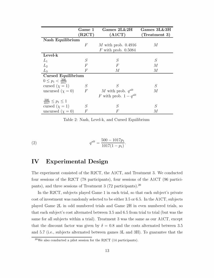
As it turns out, we can characterize the Nash equilibrium, level-k behavior, and

the cursed equilibrium, all in terms of the three strategies, S, M , and F , although

the interpretation and implications for behavior across treatments differs from our

rule-of-thumb interpretation. For our R2CT (Game 1), A1CT (Games 2L and 2H),

and Treatment 3 (Games 3L and 3H), the Nash equilibrium, level-k behavior, and the

cursed equilibrium are characterized in Table 2, all in terms of the three strategies,

S, M , and F .19 The cursed equilibrium is based on a population fraction p1 being

fully cursed (χ = 1) and the remaining fraction uncursed (χ = 0). The probability

given in Table 2, qalt, is defined as follows.

18A type (0, H) subject does not receive useful information by waiting, because the expected profitsfrom investment are always negative. A type (1, L) subject also does not receive useful informationby waiting, because the expected profits from investment are always positive.

19We are being a little loose when we refer to F , M , and S as strategies, because behavior isnot uniquely determined after unexpected contingencies that do not affect play in the NE, thecursed equilibrium, or under level-k beliefs. In our maximum likelihood estimation (section B), weare careful to specify the decisions following investment by the other subject in round 2 (after notinvesting in round 1), and following a tremble that is inconsistent with the strategy itself.

12

Game 1 Games 2L&2H Games 3L&3H(R2CT) (A1CT) (Treatment 3)

Nash EquilibriumF M with prob. 0.4916 M

F with prob. 0.5084Level-kL1 S S SL2 F F ML3 F M MCursed Equilibrium0 ≤ p1 < 500

1017

cursed (χ = 1) S S Suncursed (χ = 0) F M with prob. qalt M

F with prob. 1 − qalt

5001017

≤ p1 ≤ 1cursed (χ = 1) S S Suncursed (χ = 0) F F M

Table 2: Nash, Level-k, and Cursed Equilibrium

qalt =500 − 1017p1

1017(1 − p1).(2)

IV Experimental Design

The experiment consisted of the R2CT, the A1CT, and Treatment 3. We conducted

four sessions of the R2CT (78 participants), four sessions of the A1CT (96 partici-

pants), and three sessions of Treatment 3 (72 participants).20

In the R2CT, subjects played Game 1 in each trial, so that each subject’s private

cost of investment was randomly selected to be either 3.5 or 6.5. In the A1CT, subjects

played Game 2L in odd numbered trials and Game 2H in even numbered trials, so

that each subject’s cost alternated between 3.5 and 6.5 from trial to trial (but was the

same for all subjects within a trial). Treatment 3 was the same as our A1CT, except

that the discount factor was given by δ = 0.8 and the costs alternated between 3.5

and 5.7 (i.e., subjects alternated between games 3L and 3H). To guarantee that the

20We also conducted a pilot session for the R2CT (14 participants).

13

trials ended, without changing the equilibria, subjects were told that the trial ended

after either both subjects had invested or there were two consecutive rounds with no

investment.

Each session in all treatments consisted of two practice trials and 24 trials in which

subjects played for real money. At the start of each trial, subjects were randomly

and anonymously matched in pairs to form separate two-player markets which bore

no relation to each other. There was a new random matching from trial to trial.

Subjects were given an initial cash balance of 20 experimental currency units (ECU).

In addition, they could gain (lose) ECU in each trial, which were added to (subtracted

from) their cash balances. At the end of the session, ECU were converted into dollars

at a rate of 0.6 $/ECU in the R2CT and A1CT, and 0.5 $/ECU in Treatment 3.

Subjects were paid the resulting dollar amount or $5, whichever was greater. If a

subject’s cash balances fell below 0 at any point during the session, that subject was

paid $5 and was asked to leave.21

In order to test our interpretation of behavior, for 2 sessions of each treatment,

we followed up the investment game with some lottery problems and a questionnaire

(explained later).

Average earnings for the R2CT, the A1CT, and Treatment 3 were $26.04, $26.49,

and $24.13 respectively. Including the reading of instructions, sessions lasted between

1 hour 45 minutes and 2 hours.

Subjects in the experiment were undergraduate students at The Ohio State Uni-

versity. The sessions were held at the Experimental Economics Lab at OSU. Before

starting the trials, the experimenter read the instructions aloud as subjects read along,

seated at their computer terminals. Subjects were invited to ask questions, including

after the practice trials. Once the real trials began, no more questions were allowed.

The experiment was programmed and conducted with the software z-Tree (Urs

Fischbacher (2007)).

21This occurred for three subjects in the R2CT, for three subjects in the A1CT, and for twosubjects in Treatment 3. After a subject goes bankrupt, if the number of subjects in a session is nolonger even, one subject is randomly selected to sit out during each trial.

14

R2CTHistory (0,H) (0,L) (1,H) (1,L){} 33 (0.07) 47 (0.11) 164 (0.35) 334 (0.77){0} 18 (0.06) 28 (0.11) 43 (0.23) 37 (0.60){1} 25 (0.22) 52 (0.45) 76 (0.68) 33 (0.89){0,1} 7 (0.14) 10 (0.36) 16 (0.53) 6 (1.00){1,0} 7 (0.08) 24 (0.38) 12 (0.33) 2 (0.50){0,1,0} 1 (0.02) 2 (0.11) 3 (0.21) 0 N/Ano {0} 242 197 116 19no {1,0} 84 39 24 2no {0,1,0} 42 16 11 0Total 459 415 465 433

A1CTHistory (0,H) (0,L) (1,H) (1,L){} 28 (0.05) 72 (0.13) 207 (0.38) 447 (0.78){0} 25 (0.05) 32 (0.11) 66 (0.26) 29 (0.52){1} 16 (0.16) 105 (0.51) 53 (0.66) 59 (0.83){0,1} 13 (0.21) 12 (0.33) 14 (0.82) 4 (0.80){1,0} 13 (0.15) 44 (0.44) 11 (0.41) 7 (0.58){0,1,0} 4 (0.08) 9 (0.38) 2 (0.67) 1 (1.00)no {0} 371 218 175 22no {1,0} 74 57 16 5no {0,1,0} 45 15 1 0Total 589 564 545 574

Treatment 3History (0,H) (0,L) (1,H) (1,L){} 23 (0.06) 66 (0.15) 214 (0.46) 317 (0.79){0} 10 (0.04) 27 (0.12) 57 (0.32) 19 (0.51){1} 26 (0.28) 88 (0.57) 41 (0.59) 38 (0.83){0,1} 6 (0.16) 13 (0.43) 13 (0.52) 2 (0.50){1,0} 18 (0.27) 22 (0.33) 15 (0.54) 1 (0.13){0,1,0} 6 (0.19) 4 (0.24) 1 (0.08) 0 (0.00)no {0} 222 172 98 14no {1,0} 48 45 13 7no {0,1,0} 26 13 11 2Total 385 450 463 400

Table 3: Aggregate Actions and Frequency of Investment at each History

V Results

A Aggregate-Level Analysis

15

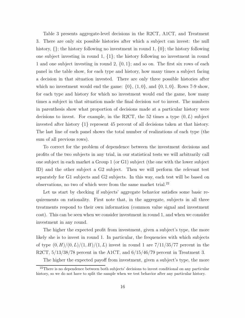
Table 3 presents aggregate-level decisions in the R2CT, A1CT, and Treatment

3. There are only six possible histories after which a subject can invest: the null

history, {}; the history following no investment in round 1, {0}; the history following

one subject investing in round 1, {1}; the history following no investment in round

1 and one subject investing in round 2, {0, 1}; and so on. The first six rows of each

panel in the table show, for each type and history, how many times a subject facing

a decision in that situation invested. There are only three possible histories after

which no investment would end the game: {0}, (1, 0}, and {0, 1, 0}. Rows 7-9 show,

for each type and history for which no investment would end the game, how many

times a subject in that situation made the final decision not to invest. The numbers

in parenthesis show what proportion of decisions made at a particular history were

decisions to invest. For example, in the R2CT, the 52 times a type (0, L) subject

invested after history {1} represent 45 percent of all decisions taken at that history.

The last line of each panel shows the total number of realizations of each type (the

sum of all previous rows).

To correct for the problem of dependence between the investment decisions and

profits of the two subjects in any trial, in our statistical tests we will arbitrarily call

one subject in each market a Group 1 (or G1) subject (the one with the lower subject

ID) and the other subject a G2 subject. Then we will perform the relevant test

separately for G1 subjects and G2 subjects. In this way, each test will be based on

observations, no two of which were from the same market trial.22

Let us start by checking if subjects’ aggregate behavior satisfies some basic re-

quirements on rationality. First note that, in the aggregate, subjects in all three

treatments respond to their own information (common value signal and investment

cost). This can be seen when we consider investment in round 1, and when we consider

investment in any round.

The higher the expected profit from investment, given a subject’s type, the more

likely she is to invest in round 1. In particular, the frequencies with which subjects

of type (0, H)/(0, L)/(1, H)/(1, L) invest in round 1 are 7/11/35/77 percent in the

R2CT, 5/13/38/78 percent in the A1CT, and 6/15/46/79 percent in Treatment 3.

The higher the expected payoff from investment, given a subject’s type, the more

22There is no dependence between both subjects’ decisions to invest conditional on any particularhistory, so we do not have to split the sample when we test behavior after any particular history.

16

likely she is to invest during some round. In particular, the frequencies with which

subjects of type (0, H)/(0, L)/(1, H)/(1, L) invest are 20/39/68/95 percent in the

R2CT, 17/49/65/95 percent in the A1CT, and 23/49/74/94 percent in Treatment

3.23 The data suggest that subjects understand when investment is profitable and

when it is not profitable, based on their signals.

We now move on to the question of whether subjects respond to the behavior of

the other subject in their trial. For each type in each treatment, we find that subjects

are considerably more likely to invest in round 2 after seeing the other subject invest

in round 1 than after seeing the other subject not invest in round 1 (compare the

frequencies of investment after history {1} and {0} in Table 3).

Now that we have established that behavior satisfies some basic requirements on

rationality, let us turn to the question of how actual investment and profit outcomes

compare with those in the NE.

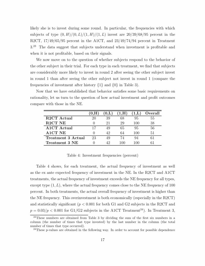
(0,H) (0,L) (1,H) (1,L) OverallR2CT Actual 20 39 68 95 55R2CT NE 0 21 29 100 38A1CT Actual 17 49 65 95 56A1CT NE 0 42 64 100 51Treatment 3 Actual 23 49 74 94 61Treatment 3 NE 0 42 100 100 61

Table 4: Investment frequencies (percent)

Table 4 shows, for each treatment, the actual frequency of investment as well

as the ex ante expected frequency of investment in the NE. In the R2CT and A1CT

treatments, the actual frequency of investment exceeds the NE frequency for all types,

except type (1, L), where the actual frequency comes close to the NE frequency of 100

percent. In both treatments, the actual overall frequency of investment is higher than

the NE frequency. This overinvestment is both economically (especially in the R2CT)

and statistically significant (p < 0.001 for both G1 and G2 subjects in the R2CT and

p = 0.03/p < 0.001 for G1/G2 subjects in the A1CT Treatment24). In Treatment 3,

23These numbers are obtained from Table 3 by dividing the sum of the first six numbers in acolumn (the number of times that type invested) by the last number in the column (the totalnumber of times that type occurred).

24These p-values are obtained in the following way. In order to account for possible dependence

17

the actual and NE frequencies of investment are equal, probably because investment

in the NE is already quite high. Summarizing:

Result 1 In the R2CT and the A1CT, the actual overall frequency of investment is

significantly higher than the NE frequency of investment. In the R2CT, overinvest-

ment is especially pronounced.

(0,H) (0,L) (1,H) (1,L) OverallR2CT Actual -0.61 0.00 0.18 3.73 0.80R2CT NE 0 0.28 0.51 3.50 1.07A1CT Actual -0.34 -0.12 0.39 3.16 0.77A1CT NE 0 0.57 0.50 3.50 1.14Treatment 3 Actual -0.31 -0.09 0.87 3.03 0.86Treatment 3 NE 0 0.50 1.30 3.50 1.33

Table 5: Average Profits per Period (in ECU)

Table 5 shows, for each treatment, the average actual profits per period as well as

the NE expected profits per period. We have:

Result 2 In all treatments, actual average profits are lower than the NE expected

profits. This difference is significant in the A1CT and in Treatment 3.25

The reason that profits are lower than the NE prediction is primarily due to un-

profitable investment by subjects with the low common-value signal, and the ensuing

unprofitable investment by subjects drawing the wrong inference.

Inspection of Tables 3 and 4 indicates that behavior in all three treatments is

remarkably similar. We employ random effects probit estimation with treatment

between investment decisions made by the same player, we perform a random effects probit esti-mation with only a constant as a right-hand-side variable. Then we test the hypothesis that thepredicted probability of investment for the average person (i.e. for someone with subject-specificrandom effect equal to 0) equals the NE ex ante probability of investment.

25p = 0.004/p = 0.042 for G1/G2 subjects in the A1CT and p < .001 for both G1 and G2 subjectsin Treatment 3. These p-values are obtained in the following way. In order to account for possibledependence between profits earned by the same player in different periods, we perform a randomeffects regression with only a constant as a right-hand-side variable. Then we test the hypothesisthat the predicted profits for the average person (i.e. for someone with subject-specific random effectequal to 0) equal the NE profits. Due to the high variance of realized profits, the difference betweenactual and NE profits is not significant in the R2CT (p = 0.203/p = 0.146 for G1/G2 subjects).

18

dummies as right-hand side variables and we cannot reject the hypothesis that there

is no treatment effect (meaning that the coefficients on all three dummies are equal)

on key history and type-contingent investment choices.

First, let us compare behavior across treatments for some key types, after the

history, {}, and after the history, {1}. In the R2CT/A1CT/Treatment 3, type

(1, L) subjects invest in round 1 77/78/79 percent of the time (p = 0.854). In the

R2CT/A1CT/Treatment 3, type (1, H) subjects invest in round 1 35/38/46 per-

cent of the time (p = 0.145).26 In the R2CT/A1CT/Treatment 3, type (1, H) sub-

jects invest after the history {1} 68/66/59 percent of the time (p = .567). In the

R2CT/A1CT/Treatment 3, type (0, L) subjects invest after history {1} 45/51/57

percent of the time (p = 0.115).

As can be seen from Table 4, the frequency of investment is also very similar

across treatments: 55/56/61 percent in the R2CT/A1CT/Treatment 3.

B Evaluating the Behavioral Theories

To evaluate which behavioral theory best explains the data, we first consider a model

in which subjects are drawn from a population of subjects who play one of the strate-

gies, F , M or S (with error). Cursed equilibrium, level-k beliefs, and insight-based

rules of thumb imply different behavior across treatments, which will allow us to

distinguish between these interpretations. Later, we will compare the values of the

likelihood functions, of our behavioral model and an extensive form QRE model.

We proceed as follows. For each treatment, for j ∈ {F, M, S}, the probability

of a subject being drawn from class j is denoted by pj. We estimate, via maximum

likelihood, the parameters pF , pM , and pS. Before proceeding to the maximum

likelihood estimation, we must specify the strategies F , M and S off the equilibrium

path. The basic principle we use is that each of these strategies prescribes correcting

one’s own departures, and choosing each action with probability 1/2 following an

unexpected choice by the other subject (i.e. after history {0, 1}).2726The p-value for the hypothesis that the coefficients on the dummies for the R2CT and Treatment

3 are equal (rather than the coefficients on all three dummies) is 0.06. R2CT and Treatment 3 arethe treatments where the NE predictions for type (1, H) differ the most (0 percent vs. 100 percent).

27Our estimates are robust to the specification of strategies off the equilibrium path. For example,we estimated a model in which, after a subject makes a mistake, she chooses to invest or not investin each subsequent round with probability one half. The estimates of pF , pM , and pS are practically

19

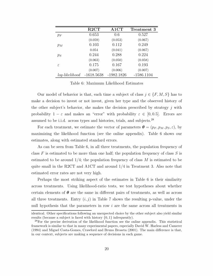
R2CT A1CT Treatment 3pF 0.653 0.6 0.527

(0.059) (0.053) (0.067)pM 0.103 0.112 0.249

0.054 (0.041) (0.067)pS 0.244 0.288 0.224

(0.063) (0.050) (0.058)ε 0.175 0.167 0.193

(0.007) (0.006) (0.007)log-likelihood -1618.5638 -1982.1826 -1586.1104

Table 6: Maximum Likelihood Estimates

Our model of behavior is that, each time a subject of class j ∈ {F, M, S} has to

make a decision to invest or not invest, given her type and the observed history of

the other subject’s behavior, she makes the decision prescribed by strategy j with

probability 1 − ε and makes an “error” with probability ε ∈ [0, 0.5]. Errors are

assumed to be i.i.d. across types and histories, trials, and subjects.28

For each treatment, we estimate the vector of parameters θ = (pF , pM , pS, ε), by

maximizing the likelihood function (see the online appendix). Table 6 shows our

estimates, along with estimated standard errors.

As can be seen from Table 6, in all three treatments, the population frequency of

class F is estimated to be more than one half; the population frequency of class S is

estimated to be around 1/4; the population frequency of class M is estimated to be

quite small in the R2CT and A1CT and around 1/4 in Treatment 3. Also note that

estimated error rates are not very high.

Perhaps the most striking aspect of the estimates in Table 6 is their similarity

across treatments. Using likelihood-ratio tests, we test hypotheses about whether

certain elements of θ are the same in different pairs of treatments, as well as across

all three treatments. Entry (i, j) in Table 7 shows the resulting p-value, under the

null hypothesis that the parameters in row i are the same across all treatments in

identical. Other specifications following an unexpected choice by the other subject also yield similarresults (because a subject is faced with history {0, 1} infrequently).

28For the precise derivation of the likelihood function see the online appendix. This statisticalframework is similar to that in many experimental papers, especially David W. Harless and Camerer(1994) and Miguel Costa-Gomes, Crawford and Bruno Broseta (2001). The main difference is that,in our context, subjects are making a sequence of decisions in each game.

20

R2CT & R2CT & A1CT & All threeA1CT Treatment 3 Treatment 3 treatments

pF 0.510 0.166 0.400 0.382pM 0.888 0.090 0.073 0.134pS 0.592 0.818 0.417 0.697ε 0.327 0.079 0.005 0.018pF , pM , pS 0.798 0.197 0.199 0.329pF , pM , pS, ε 0.708 0.088 0.009 0.041

Table 7: Hypotheses tests: p-values.

column j.

There is no strong evidence of differences in behavior across treatments. The only

p-values below 5 percent are due to the higher estimate of ε in Treatment 3.29 Most

notably, any differences in the estimates of pF across treatments are not significant.30

Let us summarize:

Result 3 (i) In all three treatments, the estimate of pF is more than 1/2; the estimate

of pS is around 1/4; the estimate of pM is quite small in the R2CT and A1CT and

is around 1/4 in Treatment 3.

(ii) The estimates of θ are very similar across treatments. In particular, any

differences in the estimates of pF across treatments are not significant.

How well do the various behavioral theories explain our estimation results for

the R2CT and A1CT treatments? (We will consider Treatment 3 shortly.) First,

consider the cursed equilibrium framework. Asymmetric cursed equilibrium, with

p1 = 0.35, predicts that (pF , pM , pS) = (0.65, 0, 0.35) in the R2CT and (pF , pM , pS) =

(0.51, 0.14, 0.35) in the A1CT, which is close to our estimates.31

Next, consider the level-k framework. Recall that, in the R2CT and A1CT, L1

plays S and L2 plays F . According to our estimates, the majority of the population

is indeed F or S. The estimates of pF and pS are nearly the same across treatments,

29The difference in the estimate of ε in Treatment 3 may be statistically significant but it is hardlyeconomically significant.

30Note that the similarity of our maximum likelihood estimates for θ across treatments is in linewith the similarity in behavior at key histories (see section A).

31In a previous version of this paper we considered a symmetric cursed equilibrium with a cursed-ness parameter, 0 < χ < 1, common to all subjects. Our MLE estimates, showing the simultaneouspresence of F and S subjects, are inconsistent with any value of χ.

21

which is what one would expect if the proportions of L1 and L2 players in the popu-

lation are stable across the treatments. Therefore, our estimates based on the R2CT

and A1CT are consistent with the level-k framework.

Finally, consider the framework in which each subject uses a rule of thumb pre-

scribing either F , M or S. Because the R2CT and A1CT are essentially the same,

in terms of the nature and difficulty of the insights discussed above, one would ex-

pect to see nearly identical behavior across the two treatments. This is indeed the

case. Therefore, our estimates based on the R2CT and A1CT are consistent with

the framework in which subjects use a rule of thumb, based on the various insights

discussed above.

Our purpose for including Treatment 3 was to distinguish between the belief-based

theories and insight-based rules of thumb. With the new parameters, a type (1, H)

subject has a dominant strategy to invest in round 1, so the strategy F is never

the optimal strategy for a risk-neutral subject within the expected utility framework,

regardless of her beliefs. If behavior in our R2CT and A1CT is driven by cursed equi-

librium or level-k beliefs, the resulting maximum likelihood estimation for Treatment

3 should show a collapse of pF .

On the other hand, suppose behavior is driven by rules of thumb based on insights

about the game. The new parameters in Treatment 3 should not affect the difficulty

of acquiring these insights. Therefore, one would expect to see a similar proportion

of F subjects as in the other two treatments. We don’t want to claim that behavior

should be completely insensitive to the new parameters. Due to the reductions of

the high investment cost and the discount factor, some subjects with foresight may

decide to invest in round 1 when their type is (1, H). However, to the extent that

behavior is mainly driven by our insights rather than based on a computation, we

would see no large drop in the estimate of pF in Treatment 3.

As we saw, the estimate of pF in Treatment 3 is above 50 percent32 and is very

similar to the estimates in the R2CT and A1CT (any differences are not significant).

This supports the view that behavior in our experiment is, to a large extent, driven

by boundedly rational rules of thumb, rather than by beliefs about the behavior of the

other subject.

32In fact, we can reject the hypothesis that pF ≤ 0.4 (0.4 is 1.96 standard errors from the estimateof pF ).

22

Our maximum likelihood estimation assumes that the strategy classes F , M , and

S are drawn from the population at the beginning of the experiment, and do not

evolve as the trials progress. This specification was made for simplicity, and because

learning issues are not our main focus. However, there seems to be some learning

going on, which sheds light on our interpretation of behavior as rules of thumb.

Random effects probit estimation is used to study the effect of the trial number on

the probability that a type (1, H) subject invests in round 1 (see equation B1 in the

online appendix). In the R2CT, the marginal effect is −0.0149 (p < 0.001); in the

A1CT, the marginal effect is −0.0105 (p = 0.003); in Treatment 3, the marginal effect

is 0.0037 (p = 0.344). The negative marginal effect in the R2CT and A1CT indicates

that subjects are “learning” to wait and observe the behavior of the other subject.33

This learning moves behavior towards the NE in the R2CT, but moves behavior away

from the NE in the A1CT. This learning could be due to a “Eureka” effect, where some

subjects suddenly acquire the insight that waiting gives them useful information about

the other subject. Why is learning absent in Treatment 3 (the estimated marginal

effect is insignificant and of the wrong sign)? Perhaps while some subjects acquire

the insight that waiting gives them useful information, other subjects realize that the

benefits are not adequate to compensate for the discounting.34 These two opposing

effects may offset each other.

Treatment 3 addresses the potential criticism that the incentives of a type (1, H)

subject are weak, so that drawing conclusions about behavior is problematic. It is true

that, in the R2CT and A1CT, the differences in the ex ante expected payoff of playing

F , M , and S are quite small (both in the NE and given the empirical frequencies of

play).35 However, in Treatment 3, the expected payoff of playing F/M/S, given the

empirical frequencies is 1.155/1.294/1.2 ECU. Therefore, the advantage of M over F

in Treatment 3 is quite substantial. Over 24 trials, the expected profit gain of playing

33This effect is large in the R2CT and A1CT. The predicted probability of investment in round 1by a type (1, H) player decreases from 0.48 in trial 1 to 0.15 in trial 24 in the R2CT and from 0.47in trial 1 to 0.23 in trial 24 in the A1CT.

34After all, even if the other subject is revealed to have the low common-value signal, the expectedloss is only 0.7 ECU in Treatment 3, while it is 1.5 ECU in the other treatments. Also, the othersubject may choose to wait with the high common-value signal, thereby weakening the inference.

35The expected payoff of playing F/M/S, given the empirical frequencies of play, is 1.084/1.057/1ECU in the R2CT and 1.09/1.10/1 ECU in the A1CT. The expected payoff of playing F/M/S, givenNE beliefs, is 1.073/1.071/1 ECU in the R2CT and 1.142/1.142/1 ECU in the A1CT.

23

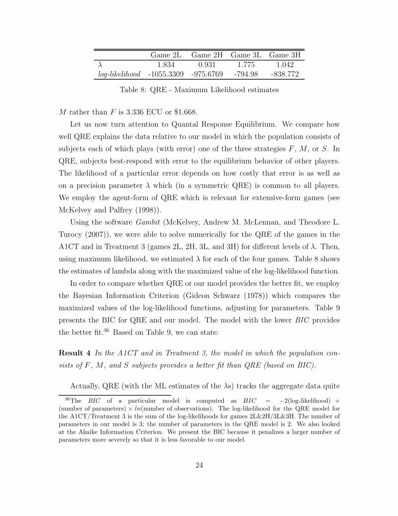
Game 2L Game 2H Game 3L Game 3Hλ 1.834 0.931 1.775 1.042log-likelihood -1055.3309 -975.6769 -794.98 -838.772

Table 8: QRE - Maximum Likelihood estimates

M rather than F is 3.336 ECU or $1.668.

Let us now turn attention to Quantal Response Equilibrium. We compare how

well QRE explains the data relative to our model in which the population consists of

subjects each of which plays (with error) one of the three strategies F , M , or S. In

QRE, subjects best-respond with error to the equilibrium behavior of other players.

The likelihood of a particular error depends on how costly that error is as well as

on a precision parameter λ which (in a symmetric QRE) is common to all players.

We employ the agent-form of QRE which is relevant for extensive-form games (see

McKelvey and Palfrey (1998)).

Using the software Gambit (McKelvey, Andrew M. McLennan, and Theodore L.

Turocy (2007)), we were able to solve numerically for the QRE of the games in the

A1CT and in Treatment 3 (games 2L, 2H, 3L, and 3H) for different levels of λ. Then,

using maximum likelihood, we estimated λ for each of the four games. Table 8 shows

the estimates of lambda along with the maximized value of the log-likelihood function.

In order to compare whether QRE or our model provides the better fit, we employ

the Bayesian Information Criterion (Gideon Schwarz (1978)) which compares the

maximized values of the log-likelihood functions, adjusting for parameters. Table 9

presents the BIC for QRE and our model. The model with the lower BIC provides

the better fit.36 Based on Table 9, we can state:

Result 4 In the A1CT and in Treatment 3, the model in which the population con-

sists of F , M , and S subjects provides a better fit than QRE (based on BIC).

Actually, QRE (with the ML estimates of the λs) tracks the aggregate data quite

36The BIC of a particular model is computed as BIC = −2(log-likelihood) +(number of parameters) × ln(number of observations). The log-likelihood for the QRE model forthe A1CT/Treatment 3 is the sum of the log-likelihoods for games 2L&2H/3L&3H. The number ofparameters in our model is 3; the number of parameters in the QRE model is 2. We also lookedat the Akaike Information Criterion. We present the BIC because it penalizes a larger number ofparameters more severely so that it is less favorable to our model.

24

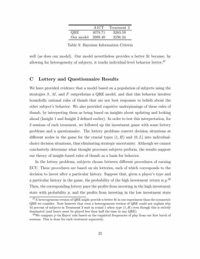
A1CT Treatment 3QRE 4078.71 3283.59Our model 3989.40 3196.34

Table 9: Bayesian Information Criteria

well (as does our model). Our model nevertheless provides a better fit because, by

allowing for heterogeneity of subjects, it tracks individual-level behavior better.37

C Lottery and Questionnaire Results

We have provided evidence that a model based on a population of subjects using the

strategies S, M , and F outperforms a QRE model, and that this behavior involves

boundedly rational rules of thumb that are not best responses to beliefs about the

other subject’s behavior. We also provided cognitive underpinnings of these rules of

thumb, by interpreting them as being based on insights about updating and looking

ahead (Insight 1 and Insight 2 defined earlier). In order to test this interpretation, for

2 sessions of each treatment, we followed up the investment game with some lottery

problems and a questionnaire. The lottery problems convert decision situations at

different nodes in the game for the crucial types (1, H) and (0, L) into individual-

choice decision situations, thus eliminating strategic uncertainty. Although we cannot

conclusively determine what thought processes subjects perform, the results support

our theory of insight-based rules of thumb as a basis for behavior.

In the lottery problems, subjects choose between different procedures of earning

ECU. These procedures are based on six lotteries, each of which corresponds to the

decision to invest after a particular history. Suppose that, given a player’s type and

a particular history in the game, the probability of the high investment return is p.38

Then, the corresponding lottery pays the profits from investing in the high investment

state with probability p, and the profits from investing in the low investment state

37A heterogeneous version of QRE might provide a better fit in our experiment than the symmetricQRE we consider. Note however that even a heterogeneous version of QRE could not explain why54 percent of subjects in Treatment 3 wait in round 1 when type (1, H) even though this is strictlydominated (and hence must be played less than half the time in any QRE).

38We compute p via Bayes’ rule based on the empirical frequencies of play from our first batch ofsessions. This is done for each treatment separately.

25

with probability 1− p.39 Lottery 1/2/3 corresponds to the decision to invest by type

(1, H) after history {}/{0}/{1}. Lottery 4/5/6 corresponds to the decision to invest

by type (0, L) after history {}/{0}/{1}.40Procedure A is simply to pay a subject according to Lottery 1.41 Hence, Procedure

A corresponds to the decision by type (1, H) to invest in round 1. To understand

Procedure B, let q be the probability that a (1, H) subject observes history {1} if

she waits until round 2.42 Procedure B is, with probability q, to let a subject choose

between Lottery 3 and getting 0 ECU for sure and, with probability 1 − q, to let a

subject choose between Lottery 2 and getting 0 ECU for sure. Hence, Procedure B

corresponds to a decision by (1, H) to wait in round 1. Procedure C is analogous to

Procedure A, except that it corresponds to the decision by type (0, L) to invest in

round 1. Procedure D is analogous to Procedure B, except that it corresponds to the

decision by type (0, L) to wait in round 1.43

The first set of lottery problems, which we call our “calibration” problems, involve

a choice between (i) being paid according to Procedure A plus receiving an amount

of money (which increases from -0.75 ECU to 1 ECU) for sure, and (ii) being paid

according to Procedure B. By finding the amount of money (the cutoff) at which each

subject switches from (ii) to (i), we can quantify by how much she values Procedure

B over Procedure A (a higher cutoff indicates a stronger preference for Procedure

B). Evaluating Procedure B requires a propensity/ability to think ahead through the

various scenarios, i.e., it requires foresight. Therefore, Procedure B is likely to be

39Actually, in the lotteries we round off p to the nearest 5 percent.40Let (X, s; Y, 1 − s) be a lottery which pays X ECU with probability s and Y ECU with

probability 1 − s. In the R2CT/A1CT/Treatment 3 Lottery 1 is (-6.5,.3;3.5,.7)/(-6.5,.3;3.5,.7)/(-5.7,.3;4.3,.7); Lottery 2 is (-5.85,.35;3.15,.65)/(-5.85,.35;3.15,.65)/(-4.56,.35;3.44,.65); Lottery 3 is(-5.85,.2;3.15,.8)/(-5.85,.2;3.15,.8)/(-4.56,.2;3.44,.8); Lottery 4 is (-3.5,.7;6.5,.3)/(-3.5,.7;6.5,.3)/(-3.5,.7;6.5,.3); Lottery 5 is (-3.15,.75;5.85,.25)/(-3.15,.75;5.85,.25)/(-2.8,.75;5.2,.25); Lottery 6 is (-3.15,.6;5.85,.4)/(-3.15,.55;5.85,.45)/(-2.8,.6;5.2,.4).

41All randomizations are performed by the computer.42We compute q via Bayes’ rule based on the empirical frequencies of play from our first batch

of sessions. This is done for each treatment separately. In the R2CT/A1CT/Treatment 3, q equals0.4/0.25/0.3.

43Let r be the probability that a (0, L) subject observes history {1} if she waits until round 2 (r iscomputed via Bayes’ rule based on the empirical frequencies of play from our first batch of sessions).Procedure D is, with probability r, to let a subject choose between Lottery 6 and getting 0 ECU forsure and, with probability 1 − r, to let a subject choose between Lottery 5 and getting 0 ECU forsure. In the R2CT/A1CT/Treatment 3, r equals 0.3/0.4/0.5.

26

unappealing for a subject without foresight.44 To the extent that waiting in round 1

by types (1, H) is driven by foresight, we may expect a correlation between a subject’s

propensity to wait in round 1 when (1, H) and her cutoff in the calibration problems.

In fact, we find that:

Result 5 A subject’s cutoff45 is a strong predictor of the probability that she waits

in round 1 when type (1, H): the marginal effect of a 0.25 ECU increase in a sub-

ject’s cutoff leads to a 12 percent increase in this probability. This effect is strongly

significant (p < 0.001).46

In the next lottery problem, subjects had to choose between Procedure A, Proce-

dure B, or getting 0 ECU for sure. This lottery problem corresponds to the decision

situation faced by a (1, H) subject in round 1.47 The top part of Table 10 shows

subjects’ choices in each treatment. Notice that the frequency with which Procedure

A is chosen in each treatment is very close to the frequency with which type (1, H)

subjects invest in round 1. Also, a subject’s choice of Procedure A is a strong pre-

dictor that she will invest in round 1 when type (1, H): the probability of investing

in round 1 is 23 percent (p = 0.009) higher for someone who chose Procedure A

(see equation B3 in the online appendix). Since the decision in the game and in the

lottery problem are framed very differently but both revolve around foresight, this

supports the view that behavior in the two settings is largely driven by whether a

subject exhibits foresight.

In the last lottery problem, subjects had to choose between Procedure C, Proce-

dure D, or getting 0 ECU for sure. This lottery problem corresponds to the decision

situation faced by a type (0, L) subject in round 1. The most interesting aspect of

44The evidence supports the view that the choice between (i) and (ii) is driven by a subject’spropensity to look ahead, rather than by a computation with errors. For example, we see notendency for lower cutoffs in Treatment 3, where the percentage of subjects whose cutoff is at least0.35 ECU is highest. However, the computed advantage of Procedure B over Procedure A is actuallylowest in Treatment 3 (and negative).

45In the R2CT/A1CT/Treatment 3 27/29/14 percent of subjects had multiple switch points. Forthese subjects, the cutoff is interpolated.

46See equation B2 in the online appendix.47The third choice, receiving 0 for sure, is analogous to a commitment in round 1 never to invest,

which is not available in the game. We included this option in the lottery problem because, if asubject lacks foresight, then she should not be expected to see that Procedure B allows her to optout later. Opting out of the lottery through procedure B requires a certain amount of foresight, butit is obvious in the game that one can choose not to invest by waiting.

27

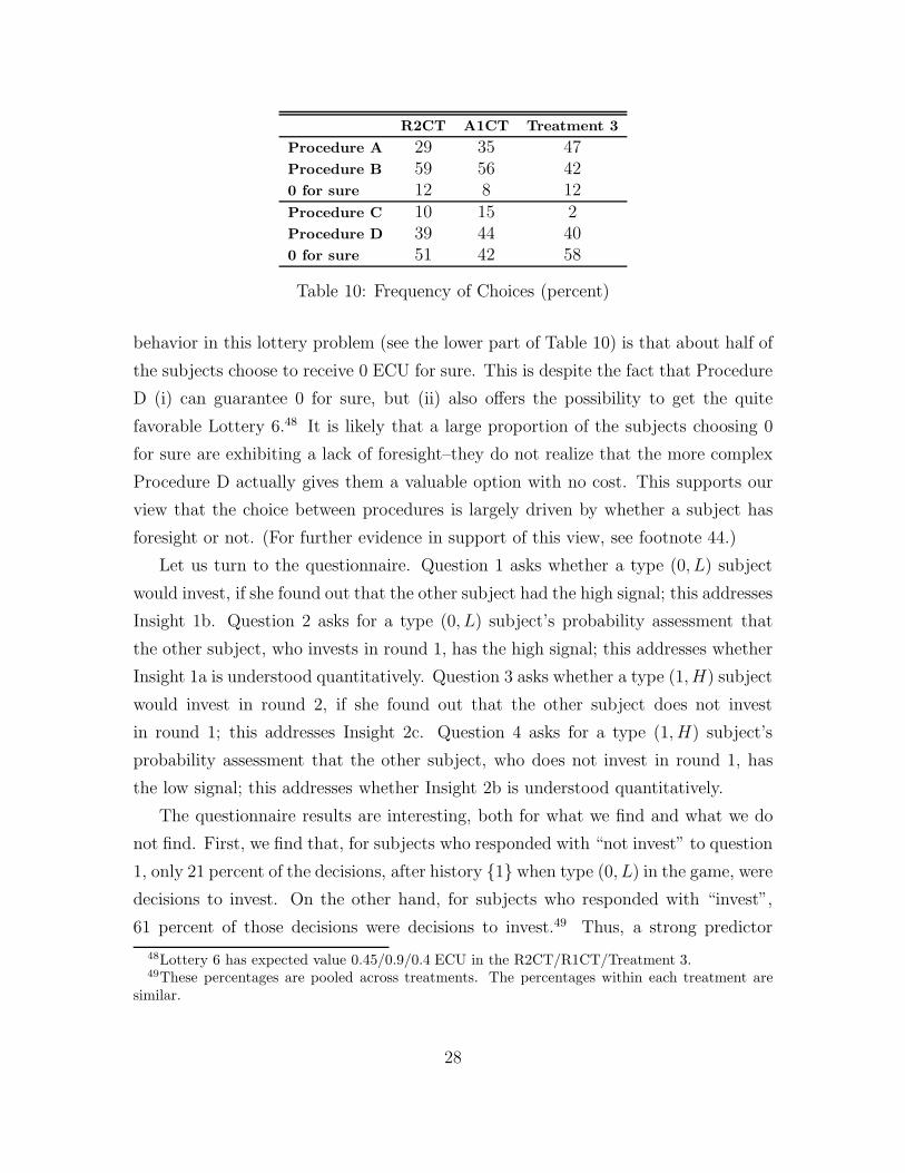
R2CT A1CT Treatment 3Procedure A 29 35 47Procedure B 59 56 420 for sure 12 8 12Procedure C 10 15 2Procedure D 39 44 400 for sure 51 42 58

Table 10: Frequency of Choices (percent)

behavior in this lottery problem (see the lower part of Table 10) is that about half of

the subjects choose to receive 0 ECU for sure. This is despite the fact that Procedure

D (i) can guarantee 0 for sure, but (ii) also offers the possibility to get the quite

favorable Lottery 6.48 It is likely that a large proportion of the subjects choosing 0

for sure are exhibiting a lack of foresight–they do not realize that the more complex

Procedure D actually gives them a valuable option with no cost. This supports our

view that the choice between procedures is largely driven by whether a subject has

foresight or not. (For further evidence in support of this view, see footnote 44.)

Let us turn to the questionnaire. Question 1 asks whether a type (0, L) subject

would invest, if she found out that the other subject had the high signal; this addresses

Insight 1b. Question 2 asks for a type (0, L) subject’s probability assessment that

the other subject, who invests in round 1, has the high signal; this addresses whether

Insight 1a is understood quantitatively. Question 3 asks whether a type (1, H) subject

would invest in round 2, if she found out that the other subject does not invest

in round 1; this addresses Insight 2c. Question 4 asks for a type (1, H) subject’s

probability assessment that the other subject, who does not invest in round 1, has

the low signal; this addresses whether Insight 2b is understood quantitatively.

The questionnaire results are interesting, both for what we find and what we do

not find. First, we find that, for subjects who responded with “not invest” to question

1, only 21 percent of the decisions, after history {1} when type (0, L) in the game, were

decisions to invest. On the other hand, for subjects who responded with “invest”,

61 percent of those decisions were decisions to invest.49 Thus, a strong predictor

48Lottery 6 has expected value 0.45/0.9/0.4 ECU in the R2CT/R1CT/Treatment 3.49These percentages are pooled across treatments. The percentages within each treatment are

similar.

28

of behavior by a type (0, L) subject after history {1} is whether she perceives that

the other subject having the high signal makes investment profitable. However, the

quantitative assessment of the probability that the other subject has the high signal

(question 2) does not have a significant effect on the probability of investment by

type (0, L) after history {1} (p = 0.153; see equation B4 in the online appendix).

Second, we find that, for subjects who responded with “not invest” to question

3, only 29 percent of the decisions, in round 1 when type (1, H) in the game, were

decisions to invest. On the other hand, for subjects who responded with “invest”,

62 percent of the decisions were decisions to invest.50 Thus, a strong predictor of

behavior by a type (1, H) subject in round 1 is whether she believes that there is an

option value of waiting (i.e., that investment is no longer profitable if the other subject

does not invest in round 1). However, the quantitative assessment of the probability

that the other subject has the low signal, after not investing in round 1, (question 4)

does not have a significant effect on the probability of investment by type (1, H) in

round 1 (p = 0.592; see equation B5) in the online appendix).51 Summarizing:

Result 6 Question 1 has a large and significant effect on the probability of investment

by type (0, L) after history {1} in the game; Question 3 has a large and significant

effect on the probability of investment by type (1, H) in round 1 in the game. However,

questions 2 and 4 have no significant predictive power for behavior in the game.

This result suggests that insights about updating and foresight play an important

role in guiding behavior in the game. However, these insights do not translate into

quantitative probability assessments.

Finally, another strong indication that behavior is driven by subjects’ ability to

acquire various insights about the game comes from a different source. We find that,

in the R2CT and A1CT, subjects’ SAT scores are a strong predictor of whether they

wait in round 1 when type (1, H) (see equation B6 in the online appendix). The

50These percentages are pooled across treatments. The percentages within each treatment aresimilar.

51There was also a question 5, which asked what a type (1, H) subject would pay to observethe other subject’s signal directly, and then decide whether to invest in round 1. We find that (i)answers are not a significant predictor of behavior in the game and (ii) the average willingness to payis 0.431 and 0.502 in the R2CT and A1CT (computed value is 0.63), while it is 0.575 in Treatment 3(computed value 0.29). Although the computed value of the information is much lower in Treatment3, average willingness to pay is higher. Thus, responses do not respond directly to computed values.

29

estimated marginal effects on the probability of waiting are 0.0013 (p < 0.001) in the

R2CT and 0.00075 (p = 0.021) in the A1CT.52 In Treatment 3, there is no significant

effect, perhaps because a high SAT score may facilitate both the acquisition of insights

as well as the realization that the benefits of waiting are not large enough.53 We also

find that subjects’ SATs are a strong predictor of whether they invest in round 2

when type (0, L) after seeing the other player invest in round 1 (see equation B7 in

the online appendix). The estimated marginal effect on the probability of following

the other subject is 0.00103 (p = 0.011).

VI Robustness of insight-based rules of thumb

In this subsection, we discuss how subjects using insight-based rules of thumb in our

games–S, M , and F subjects–would play in other experiments in the literature.

The experimental work closest to ours studies investment with endogenous timing,

where subjects observe a signal and decide whether to invest or wait. In Daniel Sgroi

(2003), subjects receive two draws from one of two urns: a “red” urn which contains

two red (R) balls and one white (W) ball, and a “white” urn which contains two

W balls and one R ball. The possible signals are either strongly red (RR), strongly

white (WW), or neutral (RW or WR). In each round, subjects either guess which

urn the draws came from, or wait (at a cost) to observe others’ guesses. Roughly 85

percent of subjects with a strong signal guess in round 1 and almost all subjects with

a neutral signal wait.

In these settings, an F subject would wait in round 1, even with a strong signal

(RR or WW). The percentage of F subjects is small (roughly 15 percent), perhaps

because there is no cost of guessing and a strong signal is extremely informative. If

an S or M subject has no clue that waiting provides a valuable option, no matter

how simple the problem, then she would always invest in round 1 (randomizing be-

tween urns with the neutral signal). However, such a literal interpretation of S and

52These marginal effects are large - in the R2CT/A1CT they imply a 41/23 percent difference inthe probability of waiting for two subjects who are two standard errors apart in their SATs.

53These findings are similar in spirit to the finding that, as the game progresses, subjects in theR2CT and A1CT learn to wait in round 1 when type (1, H), whereas subjects in Treatment 3 donot (see section B). The similarity arises when one thinks of both higher SATs and more experiencein the game as facilitating the acquisition of foresight.

30

M subjects would be a misreading of our theory, which deals with insights in com-

plex situations. A more appropriate interpretation of S and M subjects in Sgroi’s

experiment would have them guess in round 1 with a strong signal (the only complex

situation), but wait with the neutral signal.54

In Anthony Ziegelmeyer et al. (2005), each of two subjects receives a signal that is

randomly drawn from the set of integers between −4 and 4, and the subjects have to

guess whether the sum of the two signals is positive or negative. Although the Nash

equilibrium predicts perfect identification (where signals 4 and −4 guess in round 1,

signals 3 and −3 guess in round 2, etc.), a more common strategy is for signals of

absolute value 3 or 4 to guess in round 1. The authors interpret these deviations from

Nash as a cooperative attempt to internalize informational externalities.

In these settings, an F subject with the signal 3 or −3 would wait in round 1.

An S or M subject with the signal 3 or −3 would guess in round 1. Thus, we offer

an alternative explanation for why a subject with the signal 3 or −3 might guess in

round 1. Rather than an attempt at cooperation, a subject might not have a clear

insight that waiting in order to imitate is valuable, and choose a rule of thumb that

focuses on the profitability of guessing in round 1.

There is a substantial literature on herding game experiments with exogenous

timing. Obviously, these experiments do not address the issue of foresight, but Insight

1 about updating is relevant. In Lisa R. Anderson and Charles A. Holt (1997), just like

in Sgroi (2003), subjects have to guess the correct urn based on a draw from that urn

and on the observed history of others’ guesses. However, subjects make guesses in an

exogenously determined order. Information cascades, where subjects disregard their

private information and follow the majority of previous subjects, occur in 41 of the

56 periods in which an imbalance of previous guesses occurred. Goeree et al. (2007)

provide a theoretical result that the QRE of a game with sufficiently many players

will have informational cascades eventually reversing themselves and revealing the

correct urn with probability arbitrarily close to one. Experimental trials with 20 or

40 decision makers exhibit multiple, temporary cascades. In the context of Anderson

and Holt (1997) and Goeree et al. (2007), an M or F subject would go against her

54If, say, we were to increase the cost of waiting in Sgroi (2003), at some point the problem fora subject with the neutral signal would become complex. Then S and M subjects might start toinvest in round 1.

31

signal to join a cascade, while an S subject would not. If the population frequency

of S subjects is similar to our estimate of about one quarter, one would expect to see

cascades occurring after the vast majority of imbalances in Anderson and Holt (1997)

(with six subjects per market), and to see frequent cascade reversals in Goeree et al.

(2007) (with 20 or 40 subjects per market). Thus, our model provides an alternative

explanation to QRE for these experimental findings.55

Marco Cipriani and Antonio Guarino (2005) and Mathias Drehmann, Jorg Oechssler,

and Andreas Roider (2005) consider herding models where subjects decide in an ex-

ogenously determined sequence, but where the choice is whether to buy or sell an

asset. What makes this different from the urn experiments is that the asset price,

rather than being fixed, is equal to the expected asset value, given the history of

trades and the assumption that a buy (sell) decision indicates a good (bad) signal

about the asset. The Nash equilibrium is to buy with a good signal and sell with a

bad signal, without herding. Both papers find that herding is rare, but a new phe-

nomenon emerges, in which a significant minority of subjects engage in “contrarian”

behavior, selling at high prices with the good signal or buying at low prices with the

bad signal.

In these experiments, an M or F subject would follow this strategy, but an S

subject would be a contrarian.56 Thus, one explanation for contrarian behavior is

that some subjects do not update based on market histories.57

Our experimental design allows a fairly clean connection between insights, about

updating and foresight, and the corresponding behavioral rules. While it is difficult

to say exactly what strategies our S, M , and F subjects would choose in games very

different from herding games, our results are consistent with certain findings in the

55Goeree et al. (2007) find that the likelihood of abandoning a cascade falls sharply with thelength of the cascade, which suggests that even S subjects will respond to clear and compellinginformation, making the decision far less complex.

56One treatment in Drehmann, Oechssler, and Roider (2005) publicly announces previous signals,so that contrarian behavior cannot be due to beliefs about the strategies of earlier traders.

57Drehmann, Oechssler, and Roider (2005) find no evidence of heterogeneous behavior across sub-jects, which would argue against the presence of S subjects. However, each subject only participatedin 3 trials, so it was rare for a subject to have more than one or two opportunities for contrarianbehavior. Andreas Park and Sgroi (2008) ran an experiment in which contrarian behavior is ratio-nal under some circumstances. If subjects update properly, it is still the case that behavior shoulddepend on the signal and not the price. In their questionnaire, when subjects were asked whatmotivates their decisions, 44 percent said a combination of prices and signals, 31 percent said onlyprice, and 18 percent said only signal. These responses suggest heterogeneity in the population.

32

auction literature. It is known that many subjects fail to perform contingent reason-

ing, analogous to the lack of foresight exhibited by S and M subjects. For example, in

sealed-bid, second-price private-value auctions, many subjects submit bids exceeding

their value, which is a weakly dominated strategy. However, in the payoff equiva-

lent English auction, these subjects have no problem remaining in the auction until

the clock price reaches their value, and dropping out immediately thereafter. The

reason is that, although the two auctions are theoretically equivalent, the sealed-bid

auction requires the foresight to perform contingent reasoning58, while the English

auction does not. The winner’s curse in common-value auctions can involve failure

to update or failure to use foresight. In an English auction, a bidder needs to update

her assessment of the common value based on the drop-out behavior of others. In

a sealed-bid auction, a bidder needs to think ahead (with foresight) to the scenario

in which she wins, and then, within that scenario, must update her assessment of

the common value. Thus, we would expect S subjects to suffer from the winner’s

curse in both sealed-bid and English auctions, because of their inability to update,

and M subjects to suffer from the winner’s curse only in sealed-bid auctions, where

both updating and foresight are important. Charness and Levin (2007) study the

takeover game, and conclude that lack of contingent reasoning is the main cause of

the winner’s curse.59

VII Concluding Remarks

To summarize our main results, we find that subjects are more likely to invest as their

signals become more favorable, even for the subtle comparison between type (0, L)

and type (1, H). Subjects overinvest relative to the Nash benchmark. Behavior is

very similar in all three treatments.

Maximum likelihood estimates for the R2CT and A1CT are consistent with asym-

58Subjects who bid above their value in the sealed-bid auction, do not realize that the only scenarioin which the higher bid matters is one in which they pay more than their value. See Kagel, RonaldM. Harstad, and Levin (1987) as well as Kagel and Levin (2008).

59Charness and Levin show that the winner’s curse effect is greatly reduced when the game isreplaced with simpler lotteries that eliminate the need for contingent reasoning. The takeover gameis static, so contingent reasoning and Bayesian updating are intertwined. Note that our proceduresB and D are complex and multi-stage, so that the need for contingent reasoning is not eliminated.

33

metric cursed equilibrium involving a combination of fully cursed and uncursed sub-

jects. Level-k beliefs can account for these estimates as well. We can also account

for these estimates if subjects choose rules of thumb, based on insights about how to

understand the game (hindsight and foresight). To separate these explanations, we

introduce Treatment 3, in which F is strictly dominated and is inconsistent with any

theory of best responding to beliefs. We find that the proportion of F subjects does

not decline significantly, and remains above 50 percent.

Our results suggest that many subjects are not best-responding to beliefs in our

study, but this conclusion does not detract from the important contributions that

cursed equilibrium and level-k beliefs have made. Cursed equilibrium formalizes the

notion that subjects do not fully draw inferences about others’ types from their be-

havior. Level-k beliefs allow for heterogeneous beliefs about how sophisticated the

other players are, but requires best responding to those beliefs. These theories provide

important alternatives to (Bayesian) Nash equilibrium, and can account for many be-

havioral anomalies. They are particularly plausible when the primary task is to figure

out what strategies the other players will choose, and figuring out a best response is

fairly easy. In our context, a subject who understands the basic tradeoffs will have dif-

ficulty computing a best response. Also, the dynamic structure introduces new issues

of how subjects gather information from, or anticipate gathering information from,

others’ behavior over time, while cursed equilibrium and level-k beliefs are motivated

by static games.

Our model of S, M , and F subjects fits the data better than a QRE model. We

argue in section VI that insights about updating and foresight suggest corresponding

rules of thumb in herding experiments and some other experiments. However, other

games might require insights unrelated to the ones we study here. Our rules of thumb

inherently cannot provide a complete theory of bounded rationality, but they can

accurately capture behavior and perform well in an important class of environments

where insights about updating and foresight are important.

34

References

[1] Anderson, Lisa R. and Charles A. Holt. 1997. “Information Cascades in the

Laboratory.” American Economic Review, 87: 847-862.

[2] Ball, Sheryl B., Max H. Bazerman, and John S. Carroll. 1991. “An Evaluation of

Learning in the Bilateral Winner’s Curse.” Organizational Behavior and Human

Decision Processes, 48: 1-22

[3] Banerjee, Abhijit V. 1992. “A Simple Model of Herd Behavior.” Quarterly Jour-

nal of Economics, 107(3): 797-817.

[4] Bazerman, Max H. and William F. Samuelson. 1983. “I Won the Auction But

Don’t Want the Prize.” Journal of Conflict Resolution, 27: 618-634.

[5] Bikhchandani, Sushil, David Hirshleifer, and Ivo Welch. 1992. “A Theory of Fads,

Fashion, Custom, and Cultural Change as Informational Cascades.” Journal of

Political Economy, 100: 992-1026.

[6] Binmore, Ken, Jonh McCarthy, Giovanni Ponti, Larry Samuelson, and Avner

Shaked. 2002. “A Backward Induction Experiment.” Journal of Economic The-

ory, 104: 48-88.

[7] Blecherman, Barry 1996. “Is There a Winner’s Curse in the Market for Baseball

Players?” California Institute of Technology, Division of the Humanities and

Social Sciences Working Paper 966.

[8] Brunner, Christoph and Jacob K. Goeree. 2008. “Wise Crowds or Wise Minori-

ties: An Experimental Investigation.” Unpublished.

[9] Camerer, Colin F., Thomas R. Palfrey, and Brian W. Rogers. 2006. “Hetero-

geneous Quantal Response Equilibrium and Cognitive Hierarchies.” California

Institute of Technology, Division of the Humanities and Social Sciences Working

Paper 1260.

[10] Capen, Edward C., Robert V. Clapp, and William M. Campbell. 1971. “Com-

petitive Bidding in High-Risk Situations.” Journal of Petroleum Technology, 23:

641-653.

35

[11] Cassing, James and Richard W. Douglas. 1980. “Implications of the Auction

Mechanism in Baseball’s Free agent Draft.” Southern Economic Review, 47: 110-

121.

[12] Chamley, Christophe and Douglas Gale. 1994. “Information Revelation and

Strategic Delay in a Model of Investment.” Econometrica, 62(5): 1065-1085.

[13] Charness, Gary and Dan Levin. 2005. “When Optimal Choices Feel Wrong: A

Laboratory Study of Bayesian Updating, Complexity, and Psychological Affect”,

American Economic Review, 95(4): 1300-1309.

[14] Charness, Gary and Dan Levin. Forthcoming. “The Origin of the Winners Curse:

An Experimental Investigation.” American Economic Journal, Micro.

[15] Cipriani, Marco and Antonio Guarino. 2005. “Herd Behavior in a Laboratory

Financial Market.” American Economic Review, 95(5): 1427-1443.

[16] Costa-Gomes, Miguel, Vincent P. Crawford, and Bruno Broseta. 2001. “Cogni-

tion and Behavior in Normal-Form Games: An Experimental Study.” Econo-

metrica, 69: 1193-1235.

[17] Crawford, Vincent P. and Nagore Iriberri. 2007. “Level-k Auctions: Can a

Non-Equilibrium Model of Strategic Thinking Explain the Winner’s Curse and

Overbidding in Private-Value Auctions?” Econometrica, 75: 1721-70

[18] Dessauer, John P. 1981. “Book Publishing: What It Is, What It Does.” New

York: Bowker.

[19] Drehmann, Mathias, Jorg Oechssler, and Andreas Roider. 2005. “Herding and

Contrarian Behavior in Financial Markets: An Internet Experiment.” American

Economic Review 95(5), 1403-1426.

[20] Ettinger, David and Philippe Jehiel. 2008. “A Theory of Deception.”

http://www.enpc.fr/ceras/jehiel/deception.pdf

[21] Eyster, Erik and Matthew Rabin. 2005. “Cursed Equilibrium.” Econometrica,

73(5): 1623-1672.

36

[22] Fischbacher, Urs. 2007.z“-Tree: Zurich Toolbox for Ready-made Economic Ex-

periments.” Experimental Economics, 10(2): 171-178.

[23] Garratt, Rod and Todd Keister. 2006. “Bank Runs as Coordination Failures: An

Experimental Study.” Unpublished.

[24] Goeree, Jacob K., Thomas R. Palfrey, Brian W. Rogers, and Richard D. McK-

elvey. 2007. “Self-Correcting Information Cascades.” Review of Economic Studies

74(3): 733-762.

[25] Harless, David W. and Colin F. Camerer. 1994. “The Predictive Utility of Gen-

eralized Expected Utility Theories.” Econometrica, 62: 1251-1289.

[26] Hendricks, Kenneth, Richard H. Porter, and Bryan Boudreau. 1987. “Information

and Returns in OCS Auctions, 1954-1969.” Journal of Industrial Economics, 35:

517-42.

[27] Holt, Charles A., and Roger Sherman. 1994. “The Loser’s Curse and Bidder’s

Bias.” American Economic Review, 84: 642-652.

[28] Jehiel, Philippe 2001. “Limited Foresight May Force Cooperation.” Review of

Economic Studies 68: 369-391.

[29] Jehiel, Philippe 2005. “Analogy-Based Expectation Equilibrium.” Journal of

Economic Theory, 123: 81-104.

[30] Kagel, John H., Ronald M. Harstad, and Dan Levin. 1987. “Information Im-

pact and Allocation Rules in Auctions with Affiliated Private Valuations: An

Experimental Study.” Econometrica, 55: 1275-1304

[31] Kagel, John H. and Dan Levin. 1986. “The Winner’s Curse and Public Informa-

tion in Common Value Auctions.” American Economic Review, 76: 894-920.

[32] Kagel, John H. and Dan Levin. 1991. “The Winner’s Curse and Public Infor-

mation in Common Value Auctions: Reply.” American Economic Review, 81:

362-69.

37

[33] Kagel, John H. and Dan Levin. 1999. “Common Value Auctions with Insider

Information.” Econometrica, 67: 1219-1238.

[34] Kagel, John H. and Dan Levin. 2002. “Common Value Auctions and the Winner’s

Curse.” Princeton: Princeton University Press.

[35] Kagel, John H. and Dan Levin. 2008. “Comparing Efficient Multi-Object Auction

Institutions.” http://www.econ.ohio-state.edu/kagel/KL Vickrey.GEB.pdf

[36] Levin, Dan, John H. Kagel and Jean-Francois Richard. 1996. “Revenue Effects

and Information Processing in English Common Value Auctions” American Eco-

nomic Review, 86: 442-460.

[37] Levin, Dan and James Peck. Forthcoming. “Investment Dynamics with Common

and Private Values.” Journal of Economic Theory.

[38] Levis, Mario. 1990. “The Winner’s Curse Problem, Interest Costs and the Un-

derpricing of Initial Public Offerings.” Economic Journal, 100: 76-89.

[39] McKelvey, Richard D., Andrew M. McLennan, and Theodore L. Tur-

ocy. 2007. Gambit: Software Tools for Game Theory, Version 0.2007.12.04

http://gambit.sourceforge.net

[40] McKelvey, Richard D. and Thomas R. Palfrey. 1995. “Quantal Response Equi-

libria for Normal Form Games.” Games and Economic Behavior 10: 6-38.

[41] McKelvey, Richard D. and Thomas R. Palfrey. 1998. “Quantal Response Equi-

libria in Extensive Form Games.” Experimental Economics, 1: 9-41.

[42] Mead, Walter J., Asbjorn Moseidjord, and Philip E. Sorensen. 1983. “The Rate

of Return Earned by Leases Under Cash Bonus Bidding in OCS Oil and Gas

Leases.” Energy Journal, 4: 37-52.

[43] Mead, Walter J., Asbjorn Moseidjord, and Philip E. Sorensen. 1984. “Com-

petitive Bidding Under Asymmetrical Information: Behavior and Performance

in Gulf of Mexico Drainage Lease Sales, 1954-1969.” Review of Economics and

Statistics, 66: 505-08.

38

[44] Nagel, Rosemarie 1995. “Unraveling in Guessing Games: An Experimental

Study.” American Economic Review, 85: 1313-1326.

[45] Park, Andreas and Daniel Sgroi. 2008. “When Herding and Contrarianism Foster

Market Efficiency: A Financial Trading Experiment.” The Warwick Economics

Research Paper Series (TWERPS) 854, University of Warwick, Department of

Economics.

[46] Rock, Kevin. 1986. “Why New Issues are Underpriced.” Journal of Financial

Economics, 15: 187-212.

[47] Roll, Richard. 1986. “The Hubris Hypothesis of Corporate Takeovers.” Journal

of Business, 59: 197-216.

[48] Rubinstein, Ariel 1998. Modeling Bounded Rationality. Cambridge, MA and Lon-

don, England: The MIT Press.

[49] Samuelson, William F. and Max H. Bazerman. 1985. “The Winner’s Curse in

Bilateral Negotiations.” In Research in Experimental Economics (Vol. 3), ed.

Vernon Smith, Greenwich, CT: JAI Press.

[50] Schwarz, Gideon 1978. “Estimating the dimension of a model,” Annals of Statis-

tics 6(2): 461-464

[51] Sgroi, Daniel 2003. “The Right Choice at the Right Time: A Herding Experi-

ment in Endogenous Time.” Experimental Economics, 6: 159-180.

[52] Simon, Herbert A. 1972. “Theories of Bounded Rationality.” In Decisions and

Organization, eds. C.B. McGuire and Roy Radner, 161-176, Amsterdam: North

Holland.

[53] Stahl, Dale O. 2000. “Rule Learning in Symmetric Normal-Form Games: Theory

and Evidence.” Games and Economic Behavior 32: 105-138.

[54] Stahl, Dale O. 2001. “Population Rule Learning in Symmetric Normal-Form

Games: Theory and Evidence.” Journal of Economic Behavior & Organization

45: 19-35.

39

[55] Stahl, Dale O. and Ernan Haruvy. 2008. “Level-n Bounded Rationality and Dom-

inated Strategies in Normal-Form Games.” Journal of Economic Behavior &

Organization 66(2): 226-232.

[56] Stahl, Dale O. and Paul W. Wilson. 1995. “On Players’ Models of Other Players:

Theory and Experimental Evidence.” Games and Economic Behavior 10: 218-

254.

[57] Ziegelmeyer, Anthony, Kene Boun My, Jean-Christophe Vergnaud, and Marc

Willinger. 2005. “Strategic Delay and Rational Imitation in the Laboratory.”

Discussion Papers on Strategic Interaction 2005-35, Max Planck Institute of

Economics, Strategic Interaction Group.

40