hilbert space methods for control theoretic …hilbert space methods for control theoretic splines...

COMMUNICATIONS IN INFORMATION AND SYSTEMS c© 2006 International PressVol. 6, No. 1, pp. 55-82, 2006 004

HILBERT SPACE METHODS FOR CONTROL THEORETIC

SPLINES: A UNIFIED TREATMENT

Y. ZHOU∗, M. EGERSTEDT† , AND C. MARTIN‡

Abstract. In this paper we give a basic derivation of smoothing and interpolating splines and

through this derivation we show that the basic spline construction can be done through elementary

Hilbert space techniques. Smoothing splines are shown to naturally separate into a filtering problem

on the raw data and an interpolating spline construction. Both the filtering algorithm and the

interpolating spline construction can be effectively implemented. We show that a variety of spline

problems can be formulated into this common construction. By this construction we are also able to

generalize the construction of smoothing splines to continuous data, a spline like filtering algorithm.

Through the control theoretic approach it is natural to add multiple constraints and these techniques

are developed in this paper.

1. Introduction. Estimation and smoothing for data sets that contain deter-ministic and random data present difficulties not present in purely random data sets.Yet such data sets are very common in practice and if the nature of the data is notrespected conclusions may be drawn that have little relation to reality. In this pa-per we will present a unified treatment of such problems. We will extend the theoryof smoothing splines to cover such situations. Some of the techniques that we willuse have been developed in papers by Egerstedt and Martin, [4, 8, 14] and their col-leagues. The main technical contribution of this paper will be to show that many ofthese problems can be cast as minimum norm problems in suitable a Hilbert spaces.This approach unifies a series of problems that have been solved by Egerstedt, Zhou,Sun and Martin, [17, 18, 19]. Furthermore, the approach of this paper gives a unifiedtreatment of smoothing splines as developed by Wahba, [15], and the classical poly-nomial and exponential interpolating splines. The approach of this paper rests on theHilbert space methods developed by Luenberger in [7].

The theory of smoothing splines is based on the premise that a datum, α is thesum of a deterministic part, β and a random part ε. It is assumed that ε is thevalue of a random variable from some probability distribution. Smoothing splinesare designed to approximate the deterministic part by minimizing the variance ofthe random part. Often the random variable comes from measurement error. Inthe following examples the random error comes either from measurement or fromestimation based on incomplete data.

∗Department of Mathematics, Stockholm University, SE-10691 Stockholm, Sweden. E-mail:

[email protected]†Electrical and Computer Engineering, Georgia Institute of Technology, Atlanta, GA 30332, USA.

E-mail: [email protected]‡Clyde Martin, Department of Mathematics and Statistics, Texas Tech University, Lubbock, TX

79409-1042, USA. E-mail: [email protected]

55

56 Y. ZHOU, M. EGERSTEDT, AND C. MARTIN

Example 1. A very simple problem is to determine the volume of water con-tained in a playa lake in West Texas, [12]. These are transient water supplies thatbecause of their formation are almost perfectly circular. If a transect is made acrossthe center of the lake it is possible to obtain a fairly good estimate of the volume. Atthe boundary of the lake the depth of the water is 0cm. However the depth is measuredby a graduate student wading through the lake and measuring the depth at a series ofpoints. These measurement are quite random. The bottom of the lake is silted and soit is not clear where the bottom of the probe rests and the measurement is made byreading the depth of a marked probe. The data set then consists of two deterministicvalues at the boundary and a series of random numbers representing the depth at aseries of predetermined points.

Example 2. In population studies the census is taken every ten years and whethercorrect or not the values of the census are considered to be absolute for many purposes.Estimates are made of populations within a given city at irregular intervals betweenthe censuses. Thus, if it is necessary to study the growth or decline of a city over along period of time deterministic data is available at ten year intervals and estimateddata is available at shorter and often irregular time periods. The data set consists ofdeterministic census data and estimated data with random error. Estimates such asthe report by the State of California, [11], are a necessary and critical part of planningfor governments.

Example 3. For most individuals in the United States their home is the principlecomponent of their financial portfolio. The question of the value of the portfolio is ofinterest in a variety of economic indicators, [9]. When the home is purchased there isa firm monetary value that can be measured and when the home is sold there is a firmvalue. In between the value is less certain. Almost every individual can give you anestimate of the value but unless a formal appraisal is done there may be a very largeerror in the estimate. This results in a data set with a few deterministic values, thepurchase price, the selling price and formal appraisals and many random values thatare estimates by the owner.

These problems all have in common some data that can be assumed to be exactand some data that is subject to error. The goal of this paper is to find a commonframe work to treat all such linear problems.

In this paper we will consider the problem of approximating discrete or continu-ous data using the dynamics of a linear controlled system. The system may have hardconstraints such as boundary values and/or hard constraints at internal values. Thedata will be assume to noisy with known statistics. A contribution of this paper isto formulate these problems as a general class of minimum norm problems in Hilbertspace. Egerstedt, Sun and Martin, [8, 14], have formulated interpolation problemsas minimum norm problems but the general problems of smoothing spines have notto this point been so formulated. The advantage is more than conceptual in that

HILBERT SPACE METHODS FOR CONTROL THEORETIC SPLINES 57

the smoothed data is immediately available as is the smooth functional approxima-tion. Thus we will be able to split the problems into an estimation problem and aproblem of finding the interpolating splines. Both of these problems can have fastimplementations.

The outline of the paper is as follows. In Section 2 we state and solve the basicproblem of smoothing splines using Hilbert space methods to solve an associatedminimum norm problem. In Section 3 we state the basic algorithm for solving optimalcontrol problems in Hilbert space as minimal norm problems. This algorithm is thebasis for the entire paper. In Section 4 we show that interpolating splines can beconstructed using Hilbert space‘ techniques. More importantly in this section weextend the basic theory of interpolating splines to find interpolating splines withoptimal initial data. In Hilbert space this is a trivial extension of the theory but notusing other methods. In Section 5 we make a major extension of the theory to problemin which there are additional hard constraints. In one sense this amounts to changingthe spline generator to general linear boundary value problems but we show thatthese additional hard constraints can be made to define the ”constraint variety” andagain handled as minimum norm problems. In this section we solve several classicalproblems. In Section 6 we consider the related problem of smoothing continuous data.The main conceptual result is that these problems are in reality no different than theproblem of discrete data. The only complication is that they tend to involve a lot ofintegration. However we show that we can solve these filtering problems even whenthere are additional constraints that the filtered result must satisfy.

2. Statement of the basic problem. In this section we state the basic problemof smoothing splines and construct the solution. Here we show that the constructionsplits into two parts in a very natural way. Ultimately, this will allow the imple-mentation of fast algorithms for smoothing spline constructions. The basic idea ofthe construction is to define a linear variety, in a Hilbert space, that is defined bythe constraints. The data is then defined as a point in the Hilbert space and theoptimization reduces to finding the point on the affine variety that is closest (in thesense of the norm in the Hilbert space) to the data point. We know that we canconstruct this point by finding the orthogonal complement of the linear variety thatdefines the affine variety and constructing the intersection of the affine variety withthe orthogonal complement. In this process we follow Luenberger, [7].

2.1. The definitions. Let

(2.1) x = Ax + bu, y = cx, x(0) = x0

be a controllable and observable linear system with initial data x(0) = x0. We thinkof this system as the curve generator. As will be seen we achieve the smoothest


approximation if we impose the conditions for n ≥ 2

(2.2) cb = cAb = cA2b = · · · = cAn−2b = 0

where n is the dimension of the system. We impose this condition to obtain maximalsmoothness in the functions to be defined by equation (2.4). The initial data canbe chosen as part of the optimization algorithm. However, when we consider twoor multiple point value problems we will see that the initial data can be specified.Throughout we will use ( )′ to denote transpose of a matrix.

Let a data set be given as

D = {(ti, αi) : i = 1, · · · , N}and assume that ti > 0 and let T = tN . We will refer to the points ti as the “nodes.”Our goal is to find a control u(t) that minimizes

(2.3) J(u, x0) =∫ T

0

u2(t)dt + (y − α)′Q(y − α) + x′0Rx0

where Q and R are positive definite matrices. It is not strictly necessary for thesematrices to be positive definite. However, as in the case of the linear regulator, if theyare not positive definite then other conditions must be imposed to ensure a uniquesolution. We will discuss this further in Section 2.2. The vector y has components

yi = y(ti) = ceAtix0 +∫ ti

0

ceA(ti−s)bu(s)ds

and the vector α has components αi.It is convenient to define the functions

(2.4) �i(s) =

⎧⎨⎩ceA(ti−s)b, ti ≥ s,

0, ti < s.

Note that if the assumption on zeros, equation (2.2), holds then �i(s) is n − 2 timescontinuously differentiable at ti, i.e.

(2.5) �(k)i (t) =

⎧⎨⎩cAkeA(ti−s)b, ti ≥ s,

0, ti < s.

As long as cAkb = 0 the �(k)i (t) is continuous, that is until k = n − 2. We can now

write

yi = ceAtix0 +∫ T

0

�i(s)u(s)ds = ceAtix0 + 〈�i, u〉L,

where 〈�i, u〉L :=∫ T

0�i(s)u(s)ds. Now let βi := R−1eA′tic′. Then,

yi =ceAtix0 +∫ T

0

�i(s)u(s)ds

=〈βi, x0〉R + 〈�i, u〉L


where we define the inner products

〈x, w〉R = x′Rw and 〈g, h〉L =∫ T

0

g(t)h(t)dt.

Note that if we carefully take the derivatives of y(t) when u = �i(t) we have

y(2n−2)(t) =n−2∑k=0

cAn−2+kb�(n−2−k)i (t) +

∫ T

0

cA2n−1eA(t−s)b�i(s)ds.

Now this derivative is continuous but the next derivative fails to be so. Thus this y

is 2n − 2 times continuously differentiable everywhere and real analytic between thenodes.

2.2. The Hilbert space and the affine variety. Let

H = L2[0, T ]× Rn × R

N

with norm

‖(u; x; d)‖2 =∫ T

0

u2(t)dt + d′Qd + x′Rx,

and corresponding inner product

〈(u; x; d), (v; z; f)〉 =∫ T

0

u(t)v(t)dt + x′Rz + d′Qf.

Note that elements of L2[0, T ] are equivalence classes of functions. As is usual we willwork with representatives of each equivalence class. A data point in H is denoted byp. We define the linear subspace of constraints, V0, in H as

V0 = {(u; x; d) : 0 = −di + 〈βi, x〉R + 〈�i, u〉L}.

We use the notation V0 for consistency with later notation. Note that V0 is of infinitedimension since it contains a copy of L2[0, T ] and is of finite co-dimension since it isthe intersection of a finite number of co-dimension 1 subspaces. We will construct theorthogonal complement of V0 in H. Also we note that given any pair (u; x) there is acorresponding d.

Lemma 2.1. The orthogonal complement of V0 in H is

V ⊥0 = {(v; w; z) : w +

N∑i=1

〈z, ei〉Qβi = 0, v +N∑

i=1

〈z, ei〉Q�i = 0}.

Proof. By definition

V ⊥ = {(v; w; z) : 〈v, u〉L + 〈z, d〉Q + 〈w, x〉R = 0, ∀ (u; x; d) ∈ V }.


Now we have

〈z, d〉Q =N∑

i=1

〈z, ei〉Qdi =N∑

i=1

〈z, ei〉Q[〈βi, x〉R + 〈�i, u〉L]

=〈N∑

i=1

〈z, ei〉Qβi, x〉R + 〈N∑

i=1

〈z, ei〉Q�i, u〉L.

Therefore we have

0 =〈v, u〉L + 〈w, x〉R + 〈z, d〉Q

=〈v, u〉L + 〈w, x〉R + 〈N∑

i=1

〈z, ei〉Qβi, x〉R + 〈N∑

i=1

〈z, ei〉Q�i, u〉L

=〈w +N∑

i=1

〈z, ei〉Qβi, x〉R + 〈v +N∑

i=1

〈z, ei〉Q�i, u〉L.

From the definition of V0 we have that given a pair (u : x0) the there exists a d so that(u; x0, d) ∈ V0. Thus the above equality is true for u ∈ L2[0, T ] and for all x ∈ R

n

and as a consequence we must have

0 = w +N∑

i=1

〈z, ei〉Qβi and 0 = v +N∑

i=1

〈z, ei〉Q�i.

Note that the latter equality is in the sense of L2[0, T ]. The lemma follows.

2.3. The intersection of V0 ∩ (V ⊥0 + p). Before constructing the intersection

two things must be verified. The first is that V0 is nonempty and the second is thatV0 is closed. That V0 is nonempty is a consequence of the fact that every choice of u

and x determines a triple in V0. We state as a lemma the fact that V0 is closed.Lemma 2.2. V0 is a closed subspace of the Hilbert space H.Proof. Define the function with domain L2[0, T ]× R

n and range RN as

Fi((u; x)) = 〈βi, x〉R + 〈�i, u〉L.

Note that Fi is continuous since it is defined in terms of the inner products and notethat V0 is the graph of F where F is the function with components Fi. It then followsfrom the closed graph theorem that V0 is closed in H.

Since V0 is closed we have that the intersection of V0 and V ⊥0 + p consists of

a single point. This point is the solution of the optimal control problem given byequations (2.1) and (2.3).

Lemma 2.3. The intersection of V0 ∩ (V ⊥0 + p) is

V0 ∩ (V ⊥0 + p) = {(

N∑i=1

γi�i;N∑

i=1

ρiβi; (I + GQ + FQ)−1(GQ + FQ)α)},


where

γi =〈[I − (I + GQ + FQ)−1(GQ + FQ)]α, ei〉Q,

ρi =〈[I − (I + GQ + FQ)−1(GQ + FQ)]α, ei〉Q.

Proof. Equating quantities from V0 and V ⊥0 + p, (Here p = (0; 0; α) is the data

point) we have from the definition of V0 and some rearrangement of terms

di =〈βi, x〉R + 〈�i, u〉L

= −N∑

j=1

〈z, ej〉Q〈βi, βj〉R −N∑

j=1

〈z, ej〉Q〈�i, �j〉L

Now, equating d with y and z with y − α, we get

yi = −N∑

j=1

〈y − α, ej〉Q〈βi, βj〉R −N∑

j=1

〈y − α, ej〉Q〈�i, �j〉L

= − e′iGQ(y − α) − e′iFQ(y − α)

where G is the Grammian of the βi’s and F is the Grammian of the �is. Note thatsince the �is are linearly independent, F is invertible. In more compact form we have

y = −(GQ + FQ)(y − α),

or finally we have that

(2.6) (I + GQ + FQ)y = (GQ + FQ)α.

By rewriting I +GQ+FQ = (Q−1 +F +G)Q and since F and Q are positive definiteand G is positive semi-definite the matrix (I + GQ + FQ) is invertible and we find y

as linear function of the data α. This y is the optimal smoothed estimate of the dataα. Using y we can then calculate both the optimal control and the optimal initialcondition using the defining equations of the orthogonal complement.

To construct the optimal control u∗ we have from Lemma 2.1 and the identifica-tions above

u∗(t) = −N∑

i=1

〈y − α, ei〉Q�i(t)

= −N∑

i=1

〈(I + GQ + FQ)−1(GQ + FQ)α − α, ei〉Q�i(t)

=N∑

i=1

〈[I − (I + GQ + FQ)−1(GQ + FQ)b]α, ei〉Q�i(t)

The construction of the optimal initial condition is carried out in a similar manner.Thus the lemma is proved.


We summarize the results of the section with the following theorem.Theorem 2.4. Let

x = Ax + bu, y = cx

be a controllable and observable linear system with initial data x(0) = x0 and let adata set be given as

D = {(ti, αi) : i = 1, · · · , N}

and assume that ti > 0 and let T = tN . Let the cost function be given as

J(u, x0) =∫ T

0

u2(t)dt + (y − α)′Q(y − α) + x′0Rx0

where Q and R are positive definite matrices. The vector y has components

yi = y(ti) = ceAtix0 +∫ ti

0

ceA(ti−s)bu(s)ds

and the vector α has components αi. Minimizing J over u ∈ L2[0, t] and x0 ∈ Rn we

have that the optimal smoothed data is given by

(2.7) y = (I + GQ + FQ)−1(GQ + FQ)α,

the optimal control is given by

(2.8) u =N∑

i=1

〈[I − (I + GQ + FQ)−1(GQ + FQ)]α, ei〉Q�i,

and the optimal initial condition is given by

(2.9) x0 =N∑

i=1

〈[I − (I + GQ + FQ)−1(GQ + FQ)]α, ei〉Qβi

3. The basic algorithm. In the above section we have formulated and solveda problem using an algorithm based on the development in Luenberger [7] and thatis, in some sense, just an implementation of the projection theorem from the generaltheory of Hilbert space. This algorithm is extremely powerful. We will see in thispaper many problems in optimal control that can be solved by using this algorithm.We will now state the algorithm with some explanation. We begin by describing theinputs and outputs of the algorithm.INPUTS:

• a quadratic cost function in the control, possibly the initial data and in thedata;

• a given set of constraints that include a linear control system and determin-istic constraints on the solution of the control system and the initial data.


OUTPUTS:

• smoothing data y;• optimal control u;• optimal initial data x0.

The algorithm

1. Define the Hilbert space of the control, initial data and data as H = H1 ×H2×H3 where H1 is the Hilbert space of the control, H2 is the Hilbert spaceof the initial data,finite dimensional and H3 is the Hilbert space of the datawhich may be finite or infinite dimensional. The norm is based on the costfunctional.

2. Define the affine subvariety Vc of the constraints. In many of the applicationsc is replaced by the parameter from the problem, for example 0 or h.

3. Define the data as a point p in H.4. Verify that the variety is well defined in the Hilbert space. Verify that any

point evaluations are well defined. For example if f ∈ L2[0, T ] then the valuef(1) may not well defined unless it is defined in terms of the inner product.

5. Verify that the variety is closed. This is an essential step but usually in theseproblem is a consequence of the closed graph theorem.

6. Calculate the orthogonal complement of V0. This step may or may not com-plicated. It is usually straight forward.

7. Calculate the intersection of (V ⊥0 + p) ∩ Vc. This step can be complicated

because it reduces to solving a system of Linear equations derived from thedefinitions of Vc and V ⊥

0 or V ⊥0 + p. The equations can be a mix of integral

equations and finite dimensional linear equations and may involve severalparameters that must be eliminated.

8. The solution to the equations exist and is unique since we know that theintersection will contain a single point. This point is the optimal u, x0 andthe optimal output of the linear system.

This paper is an exercise in applying this algorithm to solve a series of importantproblems in the theory of control theoretic smoothing splines. There are of courseother methods of solving these problems. However, no other method seems as straightforward and as intuitive. It is basically just a generalization of the problem fromeuclidian geometry of finding a point on a given line nearest to a given point in theplane–a problem from high school geometry. The process is described by Figure (1).Note that in some problems p = 0 and these problems reduce to finding a point ofminimum norm in an affine subvariety. See [7] for many such examples.

4. Interpolating splines with initial data. For interpolating splines we arerequired to find a control that drives the output y through the points in the data set


Fig. 1. The general process for finding the point on an affine variety (Vα) in a Hilbert space

closest to a given data point (p).

D. This can be expressed in terms of additional constraints of the form

αi = 〈βi, x0〉R + 〈�i, u〉L

for i = 1, · · · , N . The goal is to find a control and an initial condition that minimizes

J(u, x0) =∫ T

0

u2(t)dt + x′0Rx0

subject to the constraints. Just as for smoothing splines we define the Hilbert spaceto be

H = L2[0, T ]× Rn.

Now the affine variety of constraints is given by

Vα = {(u; x0) : 0 = −αi + 〈βi, x0〉R + 〈�i, u〉L, i = 1, · · · , N}.

Here the goal is to find the point in Vα of minimum norm. The procedure is muchthe same as for smoothing splines. We first must verify that Vα is nonempty. Thisfollows from the hypothesized controllability of the linear system. We construct V ⊥

0

and construct the intersection

V ⊥0 ∩ Vα,

which consists of a single point, [7], provided that V0 is closed.

Lemma 4.1. V0 is closed.

Proof. Define Fi(x, w) = 〈βi, x〉R + 〈�i, w〉L. Now Fi is a continuous linearfunctional on the Hilbert space H and hence the ker(Fi) is a closed subset of H. NowV0 is the intersection of a finite number of closed subsets and hence is closed.


After some calculation we have

V ⊥0 = {(v; w) : v =

N∑i=1

τi�i, w =N∑

i=1

τiβi}.

After some more calculation we have that the optimal u is in fact given by

u =N∑

i=1

e′i(F + G)−1α�i,

and the optimal initial condition is given by

x0 =N∑

i=1

e′i(F + G)−1αβi.

the matrices F and G, the vectors βi and the elements of L2[0, T ], �i(t) are as in theprevious section. This is just a slight generalization of the construction given in [14]and hence the details are left out.

For cubic splines the classical construction reduces to solving a system of equationsof the form Λx = ρ where Λ is tridiagonal and of course this a much faster procedure.In [16] the construction of interpolating splines is reduced to solving banded matrices.However, in both cases additional constraints are required to make the problem havea unique solution. With the procedure developed here the additional constraints areunnecessary because of the optimization. Neither the classical cubic splines nor theprocedure developed in [16] can easily handle the optimal initial data.

5. Smoothing and estimation for problems with additional hard con-straints. In a series of papers Willsky and coauthors [1, 2] and Krener [6] consideredan estimation problem based on a stochastic boundary value problem. In this sectionwe consider a similar problem in which the smoothing spline is generated by linearsystem for which there are hard constraints. The constraints may occur as boundaryvalues but they may also occur as fixed internal values or even as linear operator con-straints on the solution. We will show that many of these problems can be formulatedand solved with the machinery that we have established. The basic idea is that wehave a data set in which each data point is of the form αi = f(ti) + εi where f(ti)is deterministic and the εi is the value of random variable. The goal is to producea curve (the spline) that better approximates f(t). This is, of course, a standardstatistical assumption, [15].

5.1. Two point boundary value problems. We begin by considering a gen-eral boundary value problem. Let the boundary condition be given by

(5.1) Φx(0) + Ψx(T ) = h,


where we let h ∈ Rk. This, of course, includes the classical two point boundary value

formulations and other problems of interest. We note that since

x(T ) = eAT x(0) +∫ T

0

eA(T−s)bu(s)ds,

the specific dependence on x(T ) can be removed and the boundary constraint simplybecomes

(5.2) Px(0) + Ψ∫ T

0

eA(T−s)bu(s)ds = h,

where

P := Φ + ΨeAT .

Note that if there is any solution to (5.1) then by the controllability hypothesis thereis a solution to (5.2). We hypothesize that there is at least one solution of (5.1).

We now define the Hilbert space as

H = L2[0, T ]× Rn × R

N

with norm

‖(u; x0; y)‖2 =∫ T

0

u2(t)dt + x′0Rx0 + y′Qy.

We define the constraint variety to be

Vh = {(u; x; d) : di = 〈βi, x〉R + 〈�i, u〉L, Px + Ψ∫ T

0

eA(T−s)bu(s)ds = h}.

We first prove the following lemma.Lemma 5.1. V0 is a closed subspace of H.Proof. The mapping

(u; x) → Ψ∫ T

0

eA(T−s)bu(s)ds + Px,

with domain L2[0, T ]× Rn is continuous and hence the subspace

W = {(u, x) ∈ L2[0, T ]× Rn : Px + Ψ

∫ T

0

eA(T−s)bu(s)ds = 0}

is closed. Now the mapping from W to RN defined by

di = 〈βi, x〉R + 〈�i, u〉L

is continuous and again we appeal to the closed graph theorem to finish the proof.We now construct V ⊥

0 .


Lemma 5.2. For some λ ∈ Rk,

V ⊥0 = {(v; w; z) : w = −

N∑i=1

〈z, ei〉Qβi + R−1P ′λ, v = −N∑

i=1

〈z, ei〉Q�i + (ΨeA(T−t))′λ}.

Proof. The first part of the construction is exactly the same as in subsection 2.2and from there we have

V ⊥0 = {(v; w; z) : 〈w +

N∑i=1

〈z, ei〉Qβi, x〉 + +〈v +N∑

i=1

〈z, ei〉Q�i, u〉 = 0}.

Now the relationship does not hold for all x and u but only for those x and u forwhich equation (5.2) holds. Multiplying by λ′, λ ∈ R

k, we can rewrite equation (5.2)as

(5.3) 〈R−1P ′λ, x〉R + 〈(ΨeA(T−t))′λ, u〉L = 0.

From this we conclude that

w +N∑

i=1

〈z, ei〉Qβi = R−1P ′λ,

and

v +N∑

i=1

〈z, ei〉Q�i = (ΨeA(T−t))′λ,

and the lemma follows.It remains to construct the intersection Vh ∩ (V ⊥

0 + p) to find the optimal point.This construction is technically more complicated than the simple smoothing splinebut the technique is identical.

The unique point in the intersection is defined as the solution of the followingsystem of four equations in the unknowns u, x0, y and λ, obtained by identifying x

and w with x0, d with y, and z with y + α .

u = −N∑

i=1

〈y − α, ei〉Q�i + b′eA′(T−t)Ψ′λ,(5.4)

x0 = −N∑

i=1

〈y − α, ei〉Qβi + R−1(Φ + ΨeAT )′λ,(5.5)

h = Px0 +∫ T

0

ΨeA(T−s)bu(s)ds,(5.6)

yi = 〈βi, x0〉R + 〈�i, u〉L.(5.7)

We begin by eliminating x0 and u from equation (5.7) by substituting equations (5.4)and (5.5). After some manipulation we have

yi = e′iG(y − α) − e′iF (y − α) + β′iP

′λ +∫ T

0

�i(s)b′eA′(T−s)Ψ′dsλ.


Since βi = R−1eA′tic′ let

β = R−1(eA′t1c′, · · · , eA′tN c′) =: R−1E

to obtain

y = −G(y − α) − F (y − α) + E′R−1P ′λ + Λλ,

where

Λ =∫ T

0

l(s)b′eA′(T−s)Ψ′ds.

We will now use equation (5.6) to obtain a second equation in λ and y.

h =P[−

N∑i=1

〈y − α, ei〉Qβi + R−1P ′λ]+

+∫ T

0

ΨeA(T−s)b[−

N∑i=1

〈y − α, ei〉Q�i + b′eA′(T−s)Ψ′λ]ds.

We make the following observation:

N∑i=1

〈y − α, ei〉Qβi =N∑

i=1

βie′iQ(y − α) = R−1EQ(y − α).

We now define

M =N∑

i=1

∫ T

0

ΨeA(T−s)b�i(s)e′idsQ,

and hence

N∑i=1

∫ T

0

ΨeA(T−s)b〈y − α, ei〉Q�i(s)ds = M(y − α).

Using these two constructions we then have

(5.8) h = P (−R−1EQ(y − α)) + PR−1P ′λ −−M(y − α) + ΨΓΨ′λ,

where Γ is the controllability Grammian

Γ =∫ T

0

eA(T−s)bb′eA′(T−s)ds.

By combining these two expressions linking y and λ gives the following linearequation system

(5.9)

(I + (G + F )Q −E′R−1P ′ − ΛPR−1EQ − M PR−1P ′ + ΨΓΨ′

)(y

λ

)=

((G + F )Qα

h + PR−1EQ + Mα

)


where Γ is the controllability Grammian

Γ =∫ T

0

eA(T−s)bb′eA′(T−s)ds.

Using equation (5.9) we can solve for y and for λ. These values can be used inequations (5.4) and (5.5) to uniquely determine the optimal control and the optimalinitial condition. As before we see that the optimal estimate of the data is obtainedindependently of the control.

Remark:The matrix E is a Grammian like matrix that determines if the initial datacan be recovered from sampled observational data, i.e. if x = Ax, x(0) = α, y = cx

and the output is sampled at a set of discrete points ti then the output is recoverablefrom these observations if and only if E has full rank. Thus E plays the same role asthe observability Grammian. There are no known necessary and sufficient conditionsfor E to have full rank. This problem was studied originally by Smith and Martin andwas reported in [13]. It is also interesting that the controllability Grammian arises inthe formulation of the equation (5.8). The reason for the controllability Grammian toappear is more obvious when one considers the simpler problem of optimally movingbetween affine subspaces. This problem is studied in [20].

5.2. Multiple point constraints. In this case we have a hard constraint of theform

Φ1x(r1) + · · · + Φkx(rk) = h

and the data set

D = {(ti, αi) : i = 1, · · · , N}

and we assume without loss of generality that

{ri : i = 1, · · · , k} ∪ {ti : i = 1, · · · , N} = ∅.

We again make the assumption that there exist at least one set of vectors ai such that

Φ1a1 + · · · + Φkak = h.

We construct the variety of constraints and note that we can replace x(ri) with

eArix(0) +∫ ri

0

eA(ri−s)bu(s)ds.

Thus the constraint depends only on u and x0. We use the Hilbert space

H = L2[0, T ]× Rn × R

N .


The constraint variety is

Vh = {(u; x0; y) : yi = 〈βi, x0〉 + 〈�i, u〉L,

k∑i=1

ΦieArix0 +

k∑i=1

∫ T

0

Φi�ri(s)u(s)ds = h}.

As before we construct the orthogonal complement to V0 and then determine theintersection

Vh ∩ (V ⊥0 + (0; 0; α)).

We leave this construction to the reader.

5.3. Examples. In this section we will present some examples of problems thatfit this generalized boundary value formulation. We let

A =

(0 10 0

), b =

(01

), c =

(1 0

), T = 1

t1 = 0.2, t2 = 0.3, t3 = 0.5, t4 = 0.7, t5 = 0.8

α =(0.8 0.2 0.5 1 0.3

)Q = 104I5, R = 104I2, (Ip = p × p identity matrix).

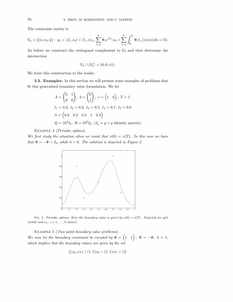
Example 4 (Periodic splines).We first study the situation when we insist that x(0) = x(T ). In this case we havethat Φ = −Ψ = I2, while h = 0. The solution is depicted in Figure 2.

0 0.1 0.2 0.3 0.4 0.5 0.6 0.7 0.8 0.9 10

0.2

0.4

0.6

0.8

1

Fig. 2. Periodic splines: Here the boundary value is given by x(0) = x(T ). Depicted are y(t)

(solid) and αi, i = 1, . . . , 4 (stars).

Example 5 (Two point boundary value problems).We now let the boundary constraint be encoded by Φ =

(1 1

), Ψ = −Φ, h = 1,

which implies that the boundary values are given by the set

{(x0, xT ) | (1, 1)x0 − (1, 1)xT = 1}.


The solution is given in Figure 3.

0 0.1 0.2 0.3 0.4 0.5 0.6 0.7 0.8 0.9 1−0.2

0

0.2

0.4

0.6

0.8

1

Fig. 3. Boundary value problem: (1, 1)x(0) − (1, 1)x(T ) = 1.

5.4. Integral constraints. In many applications ranging from statistics to med-ical there are constraints of the form∫ 1

0

y(t) dt = 1.

We will consider a simple problem with x = Ax + bu and a data set D = {(ti, αi) :i = 1, · · · , N} and we will further assume that each αi > 0. Our constraint variety isgiven by

V1 = {(u; x0; y) : yi = 〈βi, x0〉 + 〈�i, u〉, 1 =∫ T

0

y(t)dt, y(t)

= ceAtx0 +∫ t

0

eA(t−s)bu(s)ds}.

As per the algorithm we compute V ⊥0 . The definition of the orthogonal complement

gives

V ⊥0 = {(v; w, z) : 〈v, u〉 + 〈w, x0〉R + 〈z, y〉q = 0, ∀(u; x0, y) ∈ V0}.

Using the defining relation after some calculation using the first relationship in thedefinition of V0 we have

(5.10) 〈v +N∑

i=1

〈z, ei〉Q�i, u〉 + 〈w +N∑

i=1

〈z, ei〉Qβi, x0〉 = 0.

From the second and third defining relations for V0 we have

0 =∫ T

0

(eAtx0 +∫ t

0

eA(t−s)bu(s)ds)dt

=∫ T

0

eAtdtx0 +∫ T

0

∫ T

s

eA(t−s)bdtu(s)ds


Multiplying both sides by λ we have

(5.11) 0 = 〈∫ T

0

R−1eA′tdtλ, x0〉 + 〈∫ T

s

b′eA(t−s)dtλ, u〉.

Now using equations (5.10) and V ⊥0 .

V ⊥0 ={(v : w; z) : v = −

N∑i=1

〈z, ei〉Q�i +∫ T

s

b′eA(t−s)dtλ,

w = −N∑

i=1

〈z, ei〉Qβi +∫ T

0

R−1eA′tdtλ}.

Let p = (0; 0; α) where α is the vector of data.Then in order to construct (V ⊥

0 +p)∩V1 we must solve the following four equations.

yi =〈βi, x0〉 + 〈�i, u〉(5.12)

1 =∫ T

0

eAtdtx0 +∫ T

0

∫ T

s

eA(t−s)bdtu(s)ds(5.13)

u = −N∑

i=1

〈y + α, ei〉Q�i +∫ T

s

b′eA(t−s)dtλ(5.14)

x0 = −N∑

i=1

〈y + α, ei〉Qβi +∫ T

0

R−1eA′tdtλ(5.15)

The procedure for solving these four equations is exactly the same as before andwe leave the details to the reader. Use equations (5.14) and (5.15) to eliminate x0

and u from equations (5.12) and (5.13). This results in a pair of equations for λ andthe optimal y. Solve this system and substitute these values to obtain the optimal u

and x0. After some calculation the problem of finding the optimal y and λ reduces tosolving a matrix equation. The entries in the matrix must be calculated separatelyand involve some integration that can be done using standard quadrature algorithms.One y and λ are found then u and x0 are found by substituting into equations (5.14)and (5.15).

6. Continuous data. In the previous sections we developed machinery for con-structing smoothing splines with discrete data, both deterministic and random. How-ever there are many problems for which the data is continuous. EKG, ECG and EMGare primary examples for which there is a continuous data stream and often there areaspects of the data that are hidden by complexity of the stream. Smoothing splinesare an excellent tool to recover such data. In [5] smoothing splines based on B-splineswere used to recover long term trends in the stock market. In [17] it was shown thatdiscrete smoothing splines are well approximated by continuous filters which amountsto using continuous data. In this section we will develop a Hilbert space approach forsmoothing continuous data with and without additional deterministic discrete data.


6.1. The linear quadratic regulator problem. To establish the technique wewill solve the linear quadratic regulator problem and then will use the constructionfor the smoothing problems. This construction is basically the same as is given inDoolin and Martin [3]. We are given a cost function

J(u) =∫ T

0

x′(t)Qx(t) + u2(t)dt

and a controllable linear system

x = Ax + bu, x(0) = x0

and we assume that x0 is given. We also assume that the matrix Q is positive definite.We define a Hilbert space

H = L2[0, T ]× Ln2 [0, T ]

with norm

‖(u; x)‖2 =∫ T

0

x′(t)Qx(t) + u2(t)dt,

where Ln2 [0, T ] := L2[0, T ]× · · · × L2[0, T ]︸︷︷︸

n times

. Let the constraint variety be defined as

Vx0 = {(u; x) : x(t) = eAtx0 +∫ t

0

eA(t−s)bu(s)ds}.

Note again that V0 is closed by the closed graph theorem. It is seen, as for the discretecase, that we minimize the cost function by finding the point of minimum norm inVx0 . Thus we construct the orthogonal complement of V0. We have

V ⊥0 = {(v; w);

∫ T

0

x′(t)Qw(t) + u(t)v(t)dt = 0, ∀(u, ; x) ∈ V0}.

Using this definition we have

0 =∫ T

0

x′(t)Qw(t) + u(t)v(t)dt

=∫ T

0

w′(t)Q(∫ t

0

eA(t−s)bu(s)ds) + u(t)v(t)dt

=∫ T

0

∫ T

s

w′(t)Q(eA(t−s)bu(s)dtds +∫ T

0

u(s)v(s)ds

=∫ T

0

(∫ T

s

w′(t)QeA(t−s)bdt + v(s)

)u(s)ds

Thus we have

V ⊥0 = {(v; w) : v(s) = −

∫ T

s

b′eA′(t−s)Qw(t)dt}.


In order to find the intersection Vx0 ∩ V ⊥0 we must solve the following system of two

integral equations.

x(t) =eAtx0 +∫ t

0

eA(t−s)bu(s)ds(6.1)

u(s) = −∫ T

s

b′eA′(t−s)Qx(t)dt(6.2)

To solve this system we let u = −b′λ and from equation (6.2) we have

λ =∫ T

t

eA′(r−t)Qx(r)dr

and from equation (6.1) we have

x(t) = eAtx0 −∫ t

0

eA(t−s)bb′λds.

Differentiating these two equations we have the standard Hamiltonian formulation ofthe optimal control problem.

(6.3)d

dt

(x(t)λ(t)

)=

(A −bb′

−Q −A′

)(x(t)λ(t)

),

(x(0)λ(T )

)=

(x0

0

).

The solution of the equation then is done by introducing the Riccati transform. Seefor example [3] or any elementary control text.

6.2. Continuous data. As before we use a linear system

x = Ax + bu, y = cx, x(0) = x0

as the spline generator. Without loss of generality we assume that b′b = 1. We assumewe are given as our data a function

f(t) = g(t) + ε(t),

where g(t) is true underlying function and ε(t) is a represents random error. We donot need to know how the function ε is generated. We further assume that f and g

and hence ε are square integrable.We seek to minimize the following cost function. This problem is solved in great

detail in [17].

J(u, x0) =∫ T

0

u2(t)dt + x′0Rx0 +

∫ T

0

(y(t) − f(t)2)dt.

We define a Hilbert space H = L2[0, T ]× Rn × L2[0, T ] with inner product

〈(u; x; g), (v; w; h)〉 =∫ T

0

u(t)v(t)dt + x′Rw +∫ T

0

g(t)h(t)dt,


and norm

‖(u; x; g)‖2 =∫ T

0

u2(t)dt + x′Rx +∫ T

0

g2(t)dt.

Define the constraint variety to be

Vx0 = {(u(t), x0, y(t)) : y(t) = ceAtx0 +∫ t

0

ceA(t−s)bu(s)ds}

and the data point to be p = (0; 0; f(t)). Note that V0 is closed. The optimizationproblem is seen to be solved by finding the point in Vx0 that minimizes the distanceto the data point p.

In order to find this point we first construct the orthogonal complement of V inH. Now by definition we have

V ⊥0 = {(v; w; z) ∈ H : 〈u, v〉 + x′

0Rw + 〈y, z〉 = 0}.

Using this definition and the definition of y we have the following

0 =〈u, v〉 + x′0Rw + 〈y, z〉β

=∫ T

0

u(s)v(s)ds + x′0Rw +

∫ T

0

(eAtx0 +∫ t

0

ceA(t−s)bu(s))dsz(t)dt

=∫ T

0

u(s)v(s)ds + x′0Rw +

∫ T

0

(ceAtx0z(t)dt +∫ T

0

∫ T

s

ceA(t−s)bz(t)dtu(s)ds

=∫ T

0

u(s)[v(s) +∫ T

s

ceA(t−s)bz(t)dt] + x′0R[w +

∫ T

0

eA′tc′z(t)dt]

From this we conclude that

(6.4) V ⊥0 = {(v; w; z) : v(s) = −

∫ T

s

ceA(t−s)bz(t)dt, w = −∫ T

0

eA′tc′z(t)dt}.

To find the point of intersection of

(V ⊥ + p) ∩ V

we must solve the following three equations.

y(t) = ceAtx0 +∫ t

0

ceA(t−s)bu(s)ds(6.5)

u(s) = −∫ T

s

ceA(t−s)b(y(t) + f(t))dt(6.6)

x0 = −∫ T

0

eA′tc′(y(t) + f(t))dt(6.7)

Now as in the solution of the regulator problem we let

(6.8) u = −b′λ


and from equation (6.5) and (6.8) we have

x(t) = eAtx0 −∫ t

0

eA(t−s)bb′λds

and from equation (6.6) we have

λ =∫ T

s

b′beA′(t−s)c′cx(t)dt +∫ T

s

b′beA′(t−s)c′f(t))dt,

using our assumption that b′b = 1 we have the equation

λ =∫ T

s

eA′(t−s)c′cx(t)dt +∫ T

s

eA′(t−s)c′f(t))dt.

Differentiating these two equations we have the following system of equations

(6.9)d

dt

(x(t)λ(t)

)=

(A −bb′

−c′c −A′

)(x(t)λ(t)

)−(

0c′

)f(t),

(x(0)λ(T )

)=

(x0

0

)

Thus we have a forced Hamiltonian that governs the solution. This was noted andsolved in [14]. It remains to find the optimal x0. This will be done by calculating y(t)from the solution of the forced Hamiltonian. We make a change of variables definedby (

x

w

)=

(I 0

P (t) I

)(x

λ

)

Making the change of variables we have

(6.10)d

dt

(x(t)w(t)

)=

(A + b′bP (t) −bb′

R(t) −(A + bb′P (t))′

)(x(t)w(t)

)−(

0c′

)f(t),

where

(6.11) R(t) = P + PA + A′P + Pbb′P − c′c.

We now set R(t) = 0 and let P (T ) = 0 so that w(T ) = 0. Thus we have the standardRiccati equation for the linear optimal control problem of minimizing

J(u) =∫ T

0

x′c′cx + ubb′udt.

We have by solving this system of differential equations the optimal y(t) and u(t).it remains to find the optimal initial condition. We first solve and store the solutionto the Riccati equation P (t). We are guaranteed a unique solution since the systemwas assumed to be observable and controllable. We then integrate the linear system

w = −(A + bb′P (t))′w − c′f


to obtain

w(t) = −∫ T

t

φ(s, t)c′f(s)ds

and therefore we have

x(t) = −∫ t

0

φ(t, v)∫ T

v

φ(r, v)c′f(r)drdv + φ(t, 0)x0

and hence

(6.12) y(t) = −∫ t

0

cφ(t, v)∫ T

v

φ(r, v)c′f(r)drdv + cφ(t, 0)x0

From equation (6.6) we have

(6.13)u(s) =

∫ T

s

∫ s

0

∫ T

v

ceA(t−s)bcφ(s, v)φ(r, v)c′f(r)drdvdt

−∫ T

s

ceA(t−s)bf(t)dt −∫ T

s

ceA(t−s)bcφ(s, 0)x0dt.

Thus we see that u feeds back the data function f and the optimal x0 and fromequation (6.7) we see that the optimal initial data is likewise a function of the data.

x0 = −∫ T

0

eA′tc′(−∫ t

0

cφ(t, v)∫ T

v

φ(r, v)c′f(r)drdv+f(t))dt−∫ T

0

eA′tc′cφ(t, 0)dtx0

and hence we have

(∫ T

0

eA′tc′cφ(t, 0)dt + I)x0

= −∫ T

0

eA′tc′(−∫ t

0

cφ(t, v)∫ T

v

φ(r, v)c′f(r)drdv + f(t))dt.

The matrix multiplier of x0 is invertible since the solution is guaranteed to exist andto be unique from the Hilbert space formulation.

6.3. Deterministic constraints. In this subsection we consider the aboveproblem with additional constraints at specific points,

M∑i=0

Φix(ti) = h

and we assume that tM = T . This includes various forms of the boundary valueproblem (M = 1), various forms of the initial value problem (M = 0) and the problemswith constraints at internal points. We are given a measured function and the desireis to approximate it by y(t) subject to the constraints. It is possible to add otherconstraints such as constraints on integrals of y. In this case the operators Φ areintegral operators on x(t). However in this paper we will assume that the Φ are


matrices. We must verify that there is a solution (a1, · · · , aM ) of the constraintequation. If there is a solution then by controllability there is a control u that drivesthe system through the points.

We first note that the constraintM∑i=0

Φix(ti) = h can be reduced to a constraint

on u and x0.

h =M∑i=0

Φi(eAtix0 +∫ ti

0

eA(ti−s)bu(s)ds

=

(M∑i=0

ΦieAti

)x0 +

∫ T

0

(M∑i=0

ΦieA(ti−s)I[0,ti)(s)b

)u(s)ds

=Φx0 +∫ T

0

Λ(t)bu(t)dt(6.14)

where

Φ =M∑i=0

ΦieAti

and

Λ(s) =M∑i=0

ΦieA(ti−s)I[0,ti)(s),

where I[0,ti)(s) equals 1 if s ∈ [0, ti) and 0 otherwise. We see that this problem hasthe same complexity as the two point boundary value problem.

Thus we have the constraint variety defined as

Vh = {(u; x0; y) : y(t) = ceAtix0 +∫ t

0

ceA(t−s)bu(s)ds, h = Φx0 +∫ T

0

Λ(t)bu(t)dt}.

Following the previous sections we find

V ⊥0 = {(v; w; z) : v(s) = −

∫ T

s

ceA(t−s)bz(t)dt + b′Λ′λ,

w = −∫ T

0

eA′tc′z(t)dt + R−1Φ′λ}.

To find the intersection (V ⊥0 +p)∩Vh we solve the following system of four equations.

y(t) =ceAtix0 +∫ t

0

ceA(t−s)bu(s)ds(6.15)

h =Φx0 +∫ T

0

Λ(t)bu(t)dt(6.16)

u(t) = −∫ T

t

ceA(r−t)b(y(r) + f(r))dr + b′Λ′(t)λ(6.17)

x0 = −∫ T

0

eA′tc′(y(t) + f(t))dt + R−1Φ′λ(6.18)


Letting

(6.19) u(t) = −b′γ(t).

We have after some manipulation of equations (6.15) and (6.17)

x(t) =eAtix0 +∫ t

0

eA(t−s)bb′γ(s)ds,(6.20)

γ(t) = −∫ T

t

eA′(r−t)c′(y(r) + f(r))dr + Λ′(t).λ(6.21)

Differentiating equations (6.20) and (6.21) we have the system of differential equations

(6.22)d

dt

(x(t)γ(t)

)=

(A −bb′

−c′c −A′

)(x(t)γ(t)

)−(

0c′

)f(t)

with boundary conditions

x(0) = x0 and γ(T ) = 0.

As in the previous subsection we make the Riccati transform,(x

w

)=

(I 0

P (t) I

)(x

λ

),

to obtain

(6.23)d

dt

(x(t)w(t)

)=

(A + b′bP (t) −bb′

0 −(A + bb′P (t))′

)(x(t)w(t)

)−(

0c′

)f(t),

where

(6.24) P = −PA − A′P − bb′P + c′c, P (T ) = 0.

From this point the problems is exactly the same as for the two point boundary valueproblem and we leave the final construction as an exercise for the reader.

7. Conclusion. In this paper we have established a common framework forinterpolating splines and smoothing splines via a Hilbert space approach to controltheoretic splines. We have demonstrated that control theoretic splines can be used tosolve a wide variety of problems. While Willsky and colleagues, [1, 2], and Krener, [6],developed beautiful machinery based on very sophisticated stochastic analysis to solveestimation problems based on stochastic two point boundary value problems we haveshown that the same problems have elegant and simple solutions based on controltheoretic splines. Smoothing splines have along and illustrious history in statisticsthanks to the pioneering work of Grace Wahba, [15], and interpolating splines dateback to Shoenberg’s seminal paper in 1946, [10] in theory and to the early 1960s in


practice. We have been able to show that there is a common framework. Furthermorewe have been able to solve a series of problems that involve constraints on the splineand/or the data.

We recognize that not all of the interesting spline problems fall into this Hilbertspace formulation. If there are inequality constraints on the spline or its derivativeon entire intervals then we are forced to use other formulations. For example, theapproach of this paper is not really suitable for monotone smoothing splines or forsplines that are required to be in certain interval at the node points. These problemsrequire more sophisticated algorithms and have been studied by Egerstedt, Martin,Sun and Zhou in several papers, for example in [8, 14, 19].

REFERENCES

[1] M. B. Adams, A. S. Willsky, and B. C. Levy, Linear estimation of boundary value stochastic

processes. I. The role and construction of complementary models, IEEE Trans. Automat.

Control 29:9(1984), pp. 803–811.

[2] M. B. Adams, A. S. Willsky, and B. C. Levy, Linear estimation of boundary value stochastic

processes. II. 1-D smoothing problems, IEEE Trans. Automat. Control 29:9(1984), pp. 811–

821.

[3] B. Doolin and C. Martin, Differential Geometry for Control Engineers, Marcel Decker, Inc.

New York, 1990.

[4] M. Egerstedt and C. Martin, Optimal control and monotone smoothing splines, New trends

in nonlinear dynamics and control, and their applications, 279–294, Lecture Notes in Con-

trol and Inform. Sci., 295, Springer, Berlin, 2003.

[5] H. Kano, H. Nakata, and C. Martin, Optimal curve fitting and smoothing using normalized

B-splines: A tool for studying complex systems, to appear, Applied Mathematics and

Computation.

[6] A. J. Krener, Boundary value linear systems, Systems analysis (Conf., Bordeaux, 1978), pp.

149–165, Astrisque, 75-76, Soc. Math. France, Paris, 1980.

[7] D. G. Luenberger, Optimization by vector space methods, John Wiley & Sons, Inc., New

York-London-Sydney, 1969.

[8] C. F. Martin, S. Sun, and M. Egerstedt, Optimal control, statistics and path planning,

Computation and Control, VI (Bozeman, MT, 1998). Math. Comput. Modelling 33:1-

3(2001), pp. 237–253.

[9] R. F. Martin, Consumption, durable goods, and transaction costs, Dissertation, University of

Chicago, 2002.

[10] I. Schoenberg, Contributions to the problem of approximation of equidistant data by analytic

functions, Quart. Appl. Math. 4(1946), pp. 45-49.

[11] D. Sheya, M. Martindale, and L. Gage, State of California, Department of Finance, Histor-

ical City/County Population Estimates, 1991-1998, with 1990 Census Counts. Sacramento,

California, May 1998.

[12] L. M. Smith, Playas of the Great Plains. University of Texas Press, Austin, 2003.

[13] J. Smith and C. Martin, Approximation, interpolation and sampling, Differential geometry:

the interface between pure and applied mathematics (San Antonio, Tex., 1986), 227–252,

Contemp. Math., 68, Amer. Math. Soc., Providence, RI, 1987.

[14] S. Sun, M. B. Egerstedt, and C. F. Martin, Control theoretic smoothing splines, IEEE

Trans. Automat. Control, 45:12(2000), pp. 2271–2279.


[15] G. Wahba, Spline models for observational data, CBMS-NSF Regional Conference Series in Ap-

plied Mathematics, 59. Society for Industrial and Applied Mathematics (SIAM), Philadel-

phia, PA, 1990.

[16] Z. Zhang, J. Tomlinson, and C. Martin, Splines and linear control theory, Acta Applicandae

Mathematicae, 49(1997), pp. 1–34.

[17] Y. Zhou, M. Dayawansa, and C. Martin, Control theoretic smoothing splines are approximate

linear filters, Commun. Inf. Syst., 4:3(2004), pp. 253–272.

[18] Y. Zhou and C. Martin, A regularized solution to the Birkhoff interpolation problem, Com-

mun. Inf. Syst., 4(2004), pp. 89–102.

[19] Y. Zhou, M. Egersted, and C. Martin, Optimal approximation of functions, Commun. Inf.

Syst., 1:1(2001), pp. 101–112.

[20] Y. Zhou, M. Egersted, and C. Martin, Optimal trajectories between affine subspaces, sub-

mitted.

hilbert space methods for control theoretic …hilbert space methods for control theoretic splines...

Documents