highly continuous interpolants for one …...highly continuous interpolants for one-step ode solvers...
TRANSCRIPT

HIGHLY CONTINUOUS INTERPOLANTS FOR ONE-STEP ODESOLVERS AND THEIR APPLICATION TO RUNGE–KUTTA
METHODS∗
S. N. PAPAKOSTAS† AND CH. TSITOURAS‡
SIAM J. NUMER. ANAL. c© 1997 Society for Industrial and Applied MathematicsVol. 34, No. 1, pp. 22–47, February 1997 002
Abstract. We suggest a general method for the construction of highly continuous interpolantsfor one-step methods applied to the numerical solution of initial value problems of ODEs of arbitraryorder. For the construction of these interpolants one uses, along with the numerical data of thediscrete solution of a problem provided by a typical one-step method at endstep points, high-orderderivative approximations of this solution. This approach has two main advantages. It allows aneasy way of construction of high-order Runge–Kutta and Nystrom interpolants with reduced costin additional function evaluations that also preserve the one-step nature of the underlying discreteODE solver. Moreover, for problems which are known to possess a solution of high smoothness, theapproximating interpolant resembles this characteristic, a property that on occasion might be desir-able. An analysis of the stability behavior of such interpolatory processes is carried out in the generalcase. A new numerical technique concerning the accurate determination of the stability behavior ofnumerical schemes involving higher order derivatives and/or approximations of the solution fromprevious grid-points over nonequidistant meshes is presented. This technique actually turns out tobe of a wider interest, as it allows us to infer, in certain cases, more accurate results concerning thestability of, for example, the BDF formulas over variable stepsize grids. Moreover it may be used as aframework for analyzing more complex (and supposedly more promising) types of methods, as theyare the general linear methods for first- and second-order differential equations. Many particularvariants of the new method for first-order differential equations that have good prospects of findinga practical implementation are fully analyzed with respect to their stability characteristics. A de-tailed application concerning the construction of C2 and C3 continuous extensions for some fifth-and sixth-order Runge–Kutta pairs, supplemented by a detailed study of the local truncation errorcharacteristics of a class of interpolants of this type, is also provided. Various numerical examplesshow, in these cases, several advantages of the newly proposed technique with respect to functionevaluation cost and global error behavior, in comparison with others currently in use.
Key words. BDF formulas, general linear methods, interpolants, initial value problems, ODEsolvers, one-step methods, Runge–Kutta pairs
AMS subject classification. 65L05
PII. S0036142994265802
1. Introduction. We consider the νth order system of differential equations
y(ν) = f(x, y, y′, . . . , y(ν−1)
),
y (x0) = y0, y′ (x0) = y′0, . . . , y(ν−1) (x0) = y
(ν−1)0 ,
x ∈ [x0, xe] , f : R× Rm × · · · ×Rm︸ ︷︷ ︸ν
→ Rm,(1.1)
whose solution we expect to be sufficiently smooth on a neighborhood of the exactsolution. The most extensively studied numerical techniques for the solution of theproblem (1.1), both from the theoretical and the practical point of view, are thoseapplied to the cases with ν = 1, 2.
The integration methods used for the numerical solution of problem (1.1) areroughly based on the successive application, step-by-step, of a constant rule (method).
∗Received by the editors April 6, 1994; accepted for publication (in revised form) March 7, 1995.http://www.siam.org/journals/sinum/34-1/26580.html†National Technical University of Athens, Department of Mathematics, Zografou Campus, 157 80
Athens, Greece ([email protected]).‡National Air Force Academy, Dekelia TGA 1010, Athens, Greece ([email protected]).
22

HIGHLY CONTINUOUS INTERPOLANTS FOR ODE SOLVERS 23
These methods are mainly characterized, according to the number and type of infor-mation concerning the numerical solution that pass from step to step during thisprocess, as belonging to the classes of multistep (or multivalue e.t.a.), multiderivativemethods or those described as multistage (in the sense of the term used for the caseν = 1 by Hairer and Wanner in [16]). It can be seen that these methods satisfy certaintypes of algebraic order conditions. A formal presentation of these methods and therelevant algebraic theory for ν = 1 may be found, among others, in Hairer, Nørsett,and Wanner [15]. When ν = 1, the multivalue–multistage methods are also frequentlytermed general linear methods (GLMs) (see Butcher [1]). For ν > 1, the algebraictheory concerning the relevant order conditions has been studied in some particularcases; see for example Zurmuhl [35] and Hebsaker [17], [18] concerning Runge–Kutta(RK) methods for differential systems of arbitrary order.
Usually all of the above methods provide by default approximations of the theo-retical solution only at a collection of grid-points in the integration interval. Strictlymultivalue methods also provide approximations of all the derivatives of the solutionof orders at least up to ν. There are, however, cases where someone is interested inobtaining approximations at off-grid points as well. This is typically the case in thesolution (when ν = 1) of integrodifferential and delay differential equations, wherethe order of the numerical solution at the additional points, random in general, mustbe globally the same as that of the original solution, initially provided only at thegrid-points. However, this order may be one less when one is simply interested in ob-taining dense output, as for example when plotting some components of the numericalsolution.
In general, of all these methods, those that do not make use of the multistagevariant (i.e., the multivalue–multiderivative methods) are inherently based on sometype of an interpolatory scheme. For methods of this type the evaluation of thesolution at the off-grid points is, more or less, a trivial task. For all the other methodsone may employ one of two available options. The first is to use the same methodwith a different (usually smaller) stepsize in order to match exactly the specific pointat which the solution is requested each time. This option is inefficient when thefrequency of the requested off-step points is high, due to the drastic increase of the costin necessary function evaluations or even because of an emerging numerical instabilitydue to a magnification of the round-off errors. The second option is the modification ofthe original method (or the construction of a new one from scratch), which provides acontinuous solution on the whole of the integration interval. The first case of the latteroption is usually termed an interpolant or continuous extension of the original method.Alternatively, Owren and Zennaro in [25] have constructed some continuous fifth-orderRK pairs which use seven stages effectively. However, the family of continuous pairsthey define, although it uses the minimal number of stages required, does not provideany six-stage, fifth-order pair offering a discrete solution. (It is still an open questionas to whether a family of continuous pairs with these characteristics really exists.)
A popular choice for the numerical solution of the problem (1.1) when ν = 1 isthe application of an s-stage RK pair (two RK methods, usually of adjacent orders),characterized by a set of coefficients arranged in the form of the tableau
c A
b
b
where bT , bT , c ∈ Rs, A ∈ Rs×s. In addition to the approximation of the discretesolution of a problem, explicit RK methods provide approximations of the first-orderderivative at the grid-points.

24 S. N. PAPAKOSTAS AND CH. TSITOURAS
Horn in 1983 [20] was the first to propose a technique which provided a fifth-ordercontinuous extension (interpolant) to the famous 5(4)#2 pair of Fehlberg [13]. Sincethen, there has been a steady research interest in this area which has resulted inthe construction of interpolants for many RK pairs. For more up-to-date referencesin this area, see for example Verner [34]. A general framework for the constructionof interpolants for RK methods is discussed in Shampine [28] and Enright, Jackson,Nørsett and Thomsen [11]. The resulting interpolants are globally C1. A similar ap-proach may easily be followed for the construction of interpolants for explicit Nystrommethods as well (see [26] and Dormand and Prince [10]) which are globally C2.
The construction of RK pairs of order higher than four necessitates in practicethe application of a set of simplifying assumptions on the original system of algebraicorder conditions; see Curtis [7], Butcher [1]. These simplifying assumptions play adominant role in the number of additional stages required for the construction of theaccompanied interpolant, as well as for its quality. Consequently, the reconsiderationof the parent pair might also be justified, when interpolants of better quality couldbe obtained (see Calvo, Montijano, and Randez [6]; an extension and a study of thisfamily are given in [27]). A second technique is the use of multistep interpolantsas proposed in [32]. These interpolants, although they do not preserve the one-stepnature of the underlying ODE solver (in this case an RK method), they might presentan attractive alternative as they seem to offer a reduced cost in function evaluations(which, especially for low-order methods, is significant). Moreover, they are stable forarbitrary stepsize sequences chosen by the original RK code, but their local truncationerror (LTE) depends crucially on the ratios of (two or more) successive integrationsteps.
In this article we shall study the interpolation problem for an arbitrary ordersystem of differential equations, such as those described by (1.1), when the latteris solved by a general multivalue–multiderivative–multistage (MMM) method. Werestrict the formal presentation of the newly proposed technique, in the sense thatwe shall only study methods that carry past information of the numerical solutionbetween successive steps in the form of higher order derivative data that are storedin a Nordsieck-type vector [23]. This is assumed here only for notational convenience.In principle, any scheme which uses past solution points (and thus belongs to themultistep variant of MMM methods) may be transformed to an algebraically (but notanalytically) equivalent scheme involving only higher derivative data, by means of asuitable shifting operator. We term these one-step methods, and we tacitly assumethat some of the function evaluations (stages) contributing to their multistage partare, at best, strictly lower order approximations of the theoretical solution, or of someof its derivatives, at some unspecified off-grid points. When one constructs a classicalinterpolatory scheme (as those in [4], [6], [11], [28], or even [32]), one usually discardsat later steps the information contained in these off-step function evaluations of theoriginal method, as well as the information contained in the additional function eval-uations, required for the construction of the relevant continuous extension. The newinterpolation technique that we propose here carries this otherwise lost informationin the form of additional derivative data in the Nordsieck vector and uses them in away that results in the construction of interpolants of continuity higher than v. Thismight be particularly beneficial for problems whose global order of approximationdepends crucially on the smoothness of the continuous solution (for example in somedelay differential equations) or for systems of coupled differential equations when theoutput of one system is used as an input to the next.
An interpolatory process of this type, for the multistage case when ν = 1 and forthe six-stage pair FE5(4)#2, has been studied by Tsitouras and Papageorgiou [31].

HIGHLY CONTINUOUS INTERPOLANTS FOR ODE SOLVERS 25
This scheme, which provides a C2, fifth-order interpolant, uses effectively only oneadditional function evaluation, the best so far with respect to cost, for fifth-order RKpairs. (We note here that the order barriers of Owren and Zennaro [24] do not applyin this case.) While this scheme locally exhibits a rather appreciated behavior, ingeneral, when used in practical situations, it diverges. So its use is limited to onlythose cases when an interpolant is going to be used for a few number of times, forexample, when searching for the exact location of a discontinuity in the solution of aproblem.
The problem of the construction of highly continuous interpolants has also beenstudied by Higham in [19]. His work extends the interpolatory technique proposedby Shampine for RK methods [28] by including higher order derivative data amongthe points chosen for basing a highly continuous interpolant. These data are obtainedby differentiating locally an existing classical (one-step) interpolant. Hence, this ap-proach is of a different nature than that proposed here, because it does not propagateinformation of the solution other than that provided by the original RK method.Moreover, it presupposes the availability of a one-step interpolant (which, especiallyfor higher order RK pairs, is hardly the case), and consequently it does not allow anyfunction evaluation cost reduction with respect to the other classical interpolatorytechniques.
In the following, we shall describe and study the new technique in its full generalitywith respect to its stability behavior on a sequence of variable stepsizes taken bythe original one-step ODE solver. This technique may also be applied to a moregeneral class of methods (for example the BDFs or the GLMs for first- or second-order differential equations). For ν = 1, the cases which have good prospects offinding a practical implementation will be investigated in many details, particularlywith respect to their LTE behavior. We shall supplement our analysis with numericalresults concerning two schemes, the first of which offers C2 interpolants to the pairsFE5(4)#2 (Fehlberg [13]) and DP5(4) (Dormand and Prince [9]), and the other a C3
interpolant to the pair VE6(5) (Verner [33]). These new interpolatory schemes, whencompared numerically with other classical one-step interpolants for the above pairsthat have appeared in the literature, exhibit a rather appreciated behavior, as will beshown in section 6.
2. Description and stability properties of the new interpolatory tech-nique. Suppose that the application of a one-step method to the solution of problem(1.1) offers, at the grid-points x0 < x1 < · · · < xN = xe, the pth-order approximations(p ≥ ν) of the true solution and of some of its higher order derivatives y(i)
n = y(i) (xn),i = 0, 1,. . ., r, 0 ≤ n ≤ N . Usually r = ν and this is indeed the case for RK andNystrom methods. In general, for example, when some analytical derivatives of thesolution of orders exceeding v are available, we may leave a place for the possibil-ity r > ν. For ν = 1 and for the purposes of our present discussion it is irrelevantwhether these higher order derivatives are obtained by analytical differentiation of(1.1) (multiderivative methods) or are simply fictitious higher order derivative dataof the solution propagated along with it (multivalue methods; for example, Nordsieckmethods [23]).
The variable steps hi = xi − xi−1, i = 1 (1)N , at whose endpoints the evaluationof the above approximations occurs, are determined exclusively by the stepsize changemechanism, incorporated in the original ODE solver in the course of the integrationprocess.
Consider two successive integration points xn, xn+1, at which the 2 r+2, pth orderdata hiny
(i)n , hiny
(i)n+1, i = 0 (1) r are available, and suppose that we are interested in

26 S. N. PAPAKOSTAS AND CH. TSITOURAS
constructing a qth-order interpolant which will be based, among others, on thesedata. Typically q is equal to p or p − 1, and, when the original one-step methodis an essentially multistage method, for suitably large values of p it is usually q ≥p− 1 > 2 r+ 1. In such a case there is no cost-free interpolatory process immediatelyapplicable. To compensate for this, one may find a suitable number of additionalapproximations hδin y
(δi)n,pi , (pi, δi) ∈ S for i = 1, 2, . . ., λ = |S|. Classical interpolatory
processes, as those discussed in [11] and [28], are based on the points belonging to S,in addition to yn, hny′n, . . ., hrny
(r)n , yn+1, hny′n+1,. . ., hrny
(r)n+1.
Here we shall study the case in which we also have at our disposal the derivativedata hiny
(i)n , i = r + 1, r + 2,. . ., r + κ, on which we intend to base as well the newly
proposed interpolant. We assume that at some stage of the solution these derivativedata are obtained, for example, by a suitably high-order differentiation of a one-stepclassical interpolant of order p. In case there is no such interpolant available, a low-order interpolant may be used, applied, however, with a smaller stepsize. From thispoint on, these values may be easily reproduced by differentiating the interpolantunder consideration.
Setting q = 2 r + κ + λ + 1, the proposed interpolant (when t = (x− xn) /hn)assumes the form
pn (t) =r+κ∑i=0
l0,i (t)hiny(i)n +
λ∑i=1
lpiδi (t)hδin y(δi)n,pi +
r∑i=0
l1,i (t)hiny(i)n+1,(2.1)
where the polynomials li,j (t) are of the form li,j (t) = l0i,j + l1i,j t+ · · ·+ lqi,j tq and the
coefficients lki,j , k = 0 (1) q are to be determined.Define P the (q + 1)× (q + 1) matrix such that
P =(P1 P20 P3
),
with
P1 = diag (0!, 1!, . . . , (r + κ)!) ,
P2 =
(dδ1
dtδ1t0)t=p1
· · ·(dδλ
dtδλt0)t=pλ
0! 01!1! 1!
2!1!
. . ....
.... . . r!
...... (r+1)!
1!...(
dδ1
dtδ1tr+κ
)t=p1
· · ·(dδλ
dtδλtr+κ
)t=pλ
(r+κ)!(r+κ)!
(r+κ)!(r+κ−1)! · · · (r+κ)!
κ!
,
P3 =
(dδ1
dtδ1tr+κ+1
)t=p1
· · ·(dδλ
dtδλtr+κ+1
)t=pλ
(r+κ+1)!(r+κ+1)!
(r+κ+1)!(r+κ)! · · · (r+κ+1)!
(κ+1)!
......
......
...(dδ1
dtδ1tq)t=p1
· · ·(dδλ
dtδλtq)t=pλ
q!q!
q!(q−1)! · · · q!
(q−r)!
,

HIGHLY CONTINUOUS INTERPOLANTS FOR ODE SOLVERS 27
and let L be the (q + 1)× (q + 1) matrix with rows
Li =
(l00,j , l
10,j , . . . , l
q0,j
), j = i− 1, if 1 ≤ i ≤ r + κ+ 1,(
l0pj ,δj , l1pj ,δj
, . . . , lqpj ,δj
), j = i− r − κ− 1, if r + κ+ 2 ≤ i ≤ r + κ+ λ+ 1,(
l01,j , l11,j , . . . , l
q1,j
), j = i− r − κ− λ− 2, if r + κ+ λ+ 2 ≤ i ≤ q + 1.
The coefficients of the polynomials li,j (t) may be evaluated from the biorthonormalitycondition (see Davis [8]) L · P = Iq+1, where Iq+1 is the (q + 1) × (q + 1) identitymatrix. If we set a (t) = (1, t, . . . , tq)T and we define for n = 0 (1)N ,
u1n =
(yTn , hny
′Tn , . . . ,
(hrn y
(r)n
)T)T,
un =((
hr+1n y(r+1)
n
)T,(hr+2n y(r+2)
n
)T, . . . ,
(hr+κn y(r+κ)
n
)T)T,
u2n =
((hδ1n y
(δ1)n,p1
)T, . . . ,
(hδλn y
(δλ)n,pλ
)T)T,
u3n =
(yTn+1, hny
′Tn+1, . . . ,
(hrny
(r)n+1
)T)T,
zn =(u1Tn , uTn , u
2Tn , u3T
n
)T,
equation (2.1) assumes the compact form
pn (t) =((P−1a (t)
)T ⊗ Im) zn.(2.2)
So far our exposition makes use of the availability of the additional high-orderderivative information hiny
(i)n , i = (r + 1) (1) (r + κ). As we have already mentioned,
a formula for the propagation of the latter may be found by differentiating (2.1)suitably. Particularly, setting wn = hn+1/hn and rearranging the summands fori = (r + 1) (1) (r + κ), we obtain
hin+1y(i)n+1 = winh
iny
(i)n+1
= win
r+κ∑j=r+1
hjn
(di
dtil0,j (t)
)t=1
y(j)n + win
r∑j=0
hjn
(di
dtil0,j (t)
)t=1
y(j)n
+winλ∑j=1
hδjn
(di
dtilpj ,δj (t)
)t=1
y(δj)n,pj + win
r∑j=0
hjn
(di
dtil1,j (t)
)t=1
y(j)n+1.(2.3)
We define as B the matrix with columns
Bi =(dr+i
dtr+ia (t)
)t=1
, i = 1 (1)κ.
Partitioning
LB = P−1B =(DT
1 , D, DT2 , D
T3
)T,

28 S. N. PAPAKOSTAS AND CH. TSITOURAS
where D1, D, D2, DT3 are (r + 1)×κ, κ×κ, λ×κ, and (r + 1)×κ matrices, respectively,
we set
un =((u1n
)T,(u2n
)T,(u3n
)T)T,
D =(DT
1 , DT2 , D
T3
),
so that (2.3) may be written
un+1 = ((WnD)⊗ Im)un +((WnD
)⊗ Im
)un,(2.4)
where Wn = diag(wr+1n , wr+2
n , . . . , wr+κn
).
Hereafter we shall refer to the process described by (2.2), (2.4) as a highly con-tinuous interpolation method (HCIM), and we shall characterize it according to thevalues of r, κ and with an explicit reference to the data (pi, δi) as being of the form(r, κ, (p1, δ1) , (p2, δ2) , . . .).
Since the inversion of P in (2.2) is necessary only once, from the algorithmicpoint of view the new interpolatory technique imposes only one difficulty, that ofstoring at each step the values of κ, mth-length vectors (a problem which on moderncomputers with plenty of RAM, seems to be a secondary one). The special structureof P simplifies further the necessary numerical work for its inversion, observing that
P−1 =(P−1
1 −P−11 P2P
−13
0 P−13
).
An important characteristic of this technique is that the proposed interpolants are ofthe same one-step nature as the underlying discrete ODE solver.
As was mentioned in the introduction, a scheme derived in [31] may serve as anexample of a C2 interpolant of the type introduced here. Although it exhibits anappreciated local behavior in terms of cost in function evaluations, its repeated usecauses a possible divergence of the second-order derivative of the solution. Hence wehave to study this undesirable unstable behavior in more detail.
To this end we need a formula for the propagation of the errors introduced inthe scaled higher order derivatives of the solution hi y(i), i = (r + 1) (1) (r + κ). If weperform the type of interpolation described by (2.2) on the exact solution of problem(1.1) and its higher order derivatives hinψ
(i)n = hinψ
(i) (xn) we obtain analogously
ψn (t) =((P−1a (t)
)T ⊗ Im) ζn + rn (t) ,(2.5)
υn+1 = ((WnD)⊗ Im) υn +((WnD
)⊗ Im
)υn + sn,(2.6)
where for i = 1 (1)N ,
υ1n =
(ψTn , hnψ
′Tn , . . . ,
(hrnψ
(r)n
)T)T,
υn =(hr+1n
(ψ(r+1)n
)T, hr+2n
(ψ(r+2)n
)T, . . . , hr+κn
(ψ(r+κ)n
)T)T,
υ2n =
((hδ1n ψ
(δ1)n,p1
)T, . . . ,
(hδλn ψ
(δλ)n,pλ
)T)T,

HIGHLY CONTINUOUS INTERPOLANTS FOR ODE SOLVERS 29
υ3n =
(ψTn+1, hnψ
′Tn+1, . . . ,
(hrnψ
(r)n+1
)T)T,
ζn =((υ1n
)T, υTn ,
(υ2n
)T,(υ3n
)T)T,
υn =((υ1n
)T,(υ2n
)T,(υ3n
)T)T,
and rn, sn are the error terms which, from standard interpolation theory, are bothknown to behave as O (hq) (h = maxi=1(1)N (hi)).
Let
e(i)n = e(i)
n (0) = hin
(ψ(i)n − y(i)
n
),
εn = un − υn =(e(0)Tn , . . . , e(r)T
n
),
and
εn = un − υn.
Subtracting equations (2.4), (2.6), the resulting recurrence
εn+1 = ((WnD)⊗ Im) εn +((WnD
)⊗ Im
)εn − sn
leads to the formula
εn+1 =
0∏i=n(−1)
((WiD)⊗ Im)
ε0
+n−1∑i=0
i+1∏j=n(−1)
((WjD)⊗ Im)
(((WiD)⊗ Im
)εi − si
)+((WnD
)⊗ Im
)εn − sn, n = 1, . . . , (N − 1) .
(2.7)
Equation (2.7) reveals the key role played by matrix D in the error analysis of thenewly proposed interpolating method.
DEFINITION 2.1. For an HCIM of the form (r, κ, ·) we define as an interval ofstepsize change stability (w1, w2) (in short SSCSI) the interval for which there existsa consistent norm ‖·‖ on Rκ×κ such that ‖W D‖ < 1 for every w ∈ (w1, w2), whereW = diag
(wr+1, . . . , wr+κ
).
The zero SSCSI of a HCIM of the form (r, κ, ·) (denoted as 0-SSCSI) is charac-terized by the value of
w = sup‖·‖ on Rκ×κ
{w : (0, w) is an SSCSI} .
The norms in Definition 2.1 are supposed to satisfy the property ‖(WD)⊗ Im‖ =‖WD‖ for every positive integer m. While there is no definite determination of aunique SSCSI of an HCIM of the form (w1, w2) when w1 6= 0 (it is even possible thatan HCIM has no such interval), the 0-SSCSI is always uniquely determined accordingto the previous definition. Moreover, a simple continuity argument may be used inorder to show that such an interval always exists.

30 S. N. PAPAKOSTAS AND CH. TSITOURAS
DEFINITION 2.2. An HCIM is called stable with respect to stepsize changes (orsimply stable) if for this method an SSCSI of the form (w1, w2) with w1 < 1 < w2may be found.
THEOREM 2.1. Consider a one-step ODE solver applied to the solution of problem(1.1). Suppose that the errors in the initial values of u0 are O (hq) and the errors inun (introduced by the original ODE solver) are O (hp).
(i) If the original ODE solver solves exactly the special problem
y(ν) = 0, y(i) (0) = arbitrary
for i = 0, 1,. . ., ν − 1, then(a) any HCIM with ρ (D) > 1 applied to this ODE solver produces, on the
above problem, high-order derivative data that diverge;(b) if ρ (D) = 1 and µ = maxi (µi − ηi), where µi is the multiplicity of
the eigenvalues ρi of D with modulus 1 for which there exist at mostηi linearly independent eigenvectors, then the order of the high-orderderivative data produced by the HCIM is at most O (hp−µ).
(ii) If the stepsize change ratios taken by the original ODE solver belong to a(w1, w2) SSCSI for the relevant HCIM, then the global errors introduced on the high-order derivative data by this method are at most O
(hmin(p,q)
), h = maxi=0(1)N hi.
Proof. (ia) Consider a sequence of constant stepsizes h taken by the HCIMon the special problem of the hypothesis. For this particular case, since the errorsintroduced by the HCIM vanish, (2.7) leads to
εN =
(N−1∑i=0
Di
)ε0, N =
x0 − xeh
.
From linear algebra it is known that since ρ (D) > 1, some components of∑N−1i=0 Di
are at least O(ρ (D)N ) and this part of the theorem is proved.(ib) In this case some components of
∑N−1i=0 Di are at least O (Nµ) = O (h−µ).
Studying the case where ε0 = O (hp), we may see that the hypothesis is true.(ii) Applying the norm of Definition 2.1 to both sides of (2.7) we may estimate
‖εn+1‖ ≤ δn+1 ‖ε0‖+1
1− δ
(max
w∈[w1,w2]
∥∥∥Wi D∥∥∥∆1h
p + ∆2 hq
),
where δ = supw∈(w1,w2) ‖WD‖ < 1, ‖εi‖ ≤ ∆1hp, ‖si‖ ≤ ∆2h
q, i = 0 (1)N , and thequantities ∆1, ∆2 are independent of N .
Condition (i) in the hypothesis of Theorem 2.1 corresponds to one of the so-called consistency conditions of a numerical method. It is trivially satisfied by RKand Nystrom methods.
3. Full Hermit interpolation. In this section we shall first study an interpo-lation problem which arises as a special case of the more general problem introducedand studied in the previous section. Specifically, we shall study the problem of inter-polating a sufficiently smooth function y when we have at our disposal, on a prescribednumber of points
p0, p1, . . . , pm (p0 = xn, pm = xn+1),
the derivative data
hjy (pi)(j) = hjy
(j)i = hj
(djy
dxj
)x=pi
, i = 0 (1)m, j = 0 (1) ai (h = pm − p0).

HIGHLY CONTINUOUS INTERPOLANTS FOR ODE SOLVERS 31
Although from the algorithmic point of view the analysis of the previous section as itis outlined by (2.2), (2.4) seems to be adequate, for theoretical reasons the knowledgeof the expressions for each one of lij (t) (t = (x− p0) / (pm − p0)) in an explicit formis more preferable.
Let
w (x) =m∏i=1
(x− pi)ai+1 ,
ui (x) =w (x)
(x− pi)ai+1 .
It is convenient to introduce the scaled polynomials lij , li from the relations lij = hj lij ,
li (y;x) = li (x) =ai∑j=0
lij (x) y(j)i .
The Mth-order polynomial (M =∑mi=0 ai + m) that interpolates y on these points
may be expressed as
PM (x) ≡ PM (y;x) =m∑i=0
li (y;x) =m∑i=0
li (x) =m∑i=0
ai∑j=0
lij (x) y(j)i .(3.1)
Consider now for i = 0 (1)m the polynomials
PM
(li (y;x) ;x
)ui (x)
≡ li (x)ui (x)
,
which may be expanded in a Taylor series as
li (x)ui (x)
=ai∑k=0
(x− pi)k
k!dk
dxk
(li (x)ui (x)
)x=pi
.(3.2)
Since (li (y; pj)
)(k)={
0, if j 6= i,
y(k)i , if j = i,
for i, j = 0 (1)m, k = 0 (1) ai,
equation (3.2) may be written as
li (x)ui (x)
=ai∑k=0
(x− pi)k
k!dk
dxk
(y (x)ui (x)
)x=pi
.(3.3)
Substituting (3.3) in (3.1) we obtain
PM (x) =m∑i=0
ui (x)ai∑k=0
(x− pi)k
k!
k∑j=0
(k
j
)y
(j)i
(1
ui (x)
)(k−j).(3.4)
Rearranging the summation order in (3.4) we find
PM (x) =m∑i=0
ai∑j=0
ui (x)ai∑k=j
(k
j
)(x− pi)k
k!dk−j
dxk−j
(1
ui (x)
)x=pi
y(j)i ,(3.5)

32 S. N. PAPAKOSTAS AND CH. TSITOURAS
and finally comparing (3.1) with (3.5) we arrive at
lij (x) = ui (x)ai∑k=1
(k
j
)(x− pi)k
k!dk−j
dxk−j
(1
ui (x)
)x=pi
.(3.6)
Equation (3.6) gives the desired explicit form of the polynomials lij = lij/hj .
We shall now concentrate on answering the interesting question of whether thecost-free interpolation, described in the previous section, is stable; that is, if the valuew of Definition 2.1 may become greater than one for methods of the type (r, κ, ∅). Inthis case m = 1, p0 = xn, p1 = xn+1, a0 = r+κ, a1 = r, and M = 2 r+κ+1. Settingp1 = p0 + h, t = (x− p0) /h, we easily find from (3.6) that for i = 0 (1) (r + κ),
l0,i (t) = u0 (x)r+κ∑k=i
(k
i
)(x− p0)k
k!dk−i
dxk−i
(1
u0 (x)
)x=p0
= hi (t− 1)r+1r+κ∑k=i
(k
i
)tk
k!dk−i
dtk−i
(1
(t− 1)r+1
)t=0
,
from which it follows that
l0,i (t) =l0,i (t)hi
=(−1)r+1 (t− 1)r+1
r!
r+κ∑k=i
(k
i
)(k + r − i)!
k!tk.(3.7)
THEOREM 3.1. There is no stable HCIM of the form (r, κ).Proof. Differentiating (3.7) we obtain
l(j)0,i (t) =
(−1)r+1
r!
j∑k=0
(j
k
)((t− 1)r+1
)(k) r+κ∑l=i
(l
i
)(r + l − i)!
l!(tl)(j−k)
,
which after some manipulations yields
l(j)0,i (1) = (−1)r+1 (r + 1)
(j
r + 1
) r+κ∑k=max(i,j−r−1)
(k
i
)(k + r − i)!
(k − j + r − 1)!.
Substituting i→ r + i and j → r + j in (3.8) we calculate the elements of D = (di,j)
di,j = l(r+j)0,r+i (1)
= (−1)r+1 (r + 1)(r + j
r + 1
) r+κ∑k=max(r+i,j−1)
(k
r + i
)(k − i)!
(k − j + 1)!.
(3.8)
It suffices to show that the diagonal elements of D are of the same sign and eachone of them has an absolute value greater than one (because in this case the trace ofD is greater than κ and consequently its spectral radius exceeds one). The diagonalelements of D are
di,i = (−1)r+1 (r + 1)(r + i
r + 1
) r+κ∑(k=max(r+i,i−1)
=r+i )
(k
r + i
)1
k − i+ 1,
and the required result follows, since the modulus of the first summand in each oneof the above relations is greater than one and all the summands in these relations areof the same sign.

HIGHLY CONTINUOUS INTERPOLANTS FOR ODE SOLVERS 33
4. Stepsize change stability of highly continuous interpolants forRunge–Kutta methods. The negative results of Theorem 3.1 make us focus oureffort in the case of ν = r = 1 on highly continuous processes based on one or twopoints, in addition to the already available yn, hny′n, yn+1, hny′n+1. Every such ad-ditional point introduces one extra degree of freedom in the determination of theelements of matrix D while it also lowers its dimension by one as well. However, thedimension of this matrix grows in accordance with the degree of smoothness of theHCIM under consideration.
Modern RK codes usually allow stepsize change ratios between 0.5 and 1.5 andutilize pairs of orders ranging from five to eight. However, since we assume thatan arbitrary number of failures in the stepsize determination may occur, an HCIMapplicable to these pairs ought to meet two requirements. It should be based on aset of extra points allowing a 0-SSCSI of the form (0, w) with w ≥ 1.5. Moreover,these points should provide an HCIM with adequately small LTE coefficients of boththe continuous solution and its higher order derivatives at the endstep points. Inthis section we shall concentrate on answering the first of these two questions. Tothis end extensive use will be made of the J-norm associated with ‖·‖, introduced bythe relation ‖A‖J =
∥∥JAJ−1∥∥, where A, J ∈ Rκ×κ. We note that this norm fulfills
the requirements of Definition 2.1, and it is always defined in terms of some otherconsistent norm in Rκ×κ. In general J may differ from the matrix bringing A to itsJordan canonical form.
Let I = (0, w) be the 0-SSCSI of an HCIM of the form (r, κ, ·) characterized bythe matrix D and let
Is = (0, ws) =(
0, supw{w : ρ (WD) < 1 ∀w ∈ (0, w)}
)and
I‖·‖,J =(0, w‖·‖,J
)=(
0, supw{w : ‖WD‖J < 1 ∀w ∈ (0, w)}
),
where W = diag(wr+1, wr+2, . . . , wr+κ
). Then it is fairly straightforward to see that,
for any J ∈ Rκ×κ and ‖·‖ on Rκ×κ, I‖·‖,J ⊆ I ⊆ Is.Consequently, if we define for a given norm ‖·‖,
I l,‖·‖ =(0, wl,‖·‖
)=(
0, supJ∈Rκ×κ
{w‖·‖,J
}),
then
I l,‖·‖ ⊆ I ⊆ Is.(4.1)
Finally, in most cases the problem of finding the appropriate norm for an accurateestimation of the 0-SSCSI of an HCIM may be reduced essentially to that of solvingthe following maximization problem:
wl,‖·‖ = maxJ∈Rκ×κ
{w : w is the first positive root of ‖WD‖J = 1}(4.2)
for some ‖·‖ on Rκ×κ.It may be shown that the above maximum really exists as, in this case, w is a
continuous function of the elements of J and on a sufficiently small region around zero

34 S. N. PAPAKOSTAS AND CH. TSITOURAS
the value of ‖W D‖J is less than one. In the literature similar problems have appearedin the past when one tries to find accurate 0-SSCSIs for the BDF and the Nordsieck–Adams–Bashforth methods; see Grigorieff [14]; Calvo, Grande, and Grigorieff [2];Skeel and Jackson [30]; Calvo, Lisbona, and Montijano [3]. In these cases and forhigh-order formulas, one is also forced to revert to the use of numerical techniques.However, the bulk of the numerical work necessary in these cases is much lighterbecause the resulting matrices are characterized exclusively by constant coefficients,while in our case they depend on the values of the off-step points incorporated inthe HCIM. The most optimistic results have appeared in [2], [3] and were obtainedby using the J-norm evaluated from the Jordan canonical form of the relevant D (w)matrix for w = ws. The norm used in these cases was associated with the l1 norm ofa matrix.
In our case we tried two approaches for the solution of this problem. First wenumerically solved (4.2) directly. This approach allows a large number of free param-eters in J . Alternatively we reduced the problem to a single degree of freedom byrestricting J as the Jordan canonical form of WD, evaluated at some w ∈ (0, ws).For comparison purposes we compared the results obtained by associating the J-normsuccessively with each one of l1, l2, l∞.
Contrary to our initial expectations, we found that the second of the above tech-niques not only was, as expected, faster, but was also giving larger 0-SSCSIs thanthe first. We also found that in almost all cases it is preferable to associate the J-norm with the Euclidean norm. Hence, hereafter for convenience we use the notationwl = wl,l2 , I l = I l,l2 .
For illustration purposes we shall compare the values (0, w) obtained by both themethod of Calvo et al. [3] and the new method used here on an implicit three-stepNordsieck–Adams method. An upper bound for the value of w may be found to bethe number ws = 1.439. While the method of Calvo et al. predicts a poor 0.39, thenew method verifies that w cannot be less than wl = 1.41, which is very satisfactoryindeed.
In the rest of this section we shall present some numerical results related tothe stability characteristics of some candidate solutions, alternative to the classicaltechniques, for the problem of HCIM construction for RK pairs of orders 5, 6, 7, and8 that arise most frequently in practice. In the following, explicit reference of D withrespect to an HCIM of the type (r, κ, ·) will be emphasized by writing D (r, κ, ·).
Concerning fifth-order RK pairs the intervals I, I l, and Is are identical, particu-larly
D (1, 1, (p, 1)) =(p− 1) (5 p− 2)p (5 p− 3)
.
From this relation we see that for a 0-SSCSI (0, 1.5) we may select any value of
p ∈((
27−√
129)/50,
(15−
√105)/10)⋃((
27 +√
129)/50,∞
).
Moreover, when p = 2/5, the HCIM of the above form has the whole of the positivereal axis as a 0-SSCSI. Similarly, as D (1, 1, (p, 0)) = 1 − 1/p, we see that an SSCSIcontaining (0, 1.5) may be obtained when p ∈ (3/5,∞). No selection of p leads to aninfinite 0-SSCSI in this case.
Figure 1 represents a plot of the safe values wl of the 0-SSCSIs for an HCIM of theform (1, 1, (p, 1)) relative to p. Figure 2 is the respective plot when an HCIM of the

HIGHLY CONTINUOUS INTERPOLANTS FOR ODE SOLVERS 35
FIG. 1. The lower bound wl of the 0-SSCSI for an HCIM of the form (1, 1, (p, 1)). Thecontinuous line represents the safe lower bound for w, estimated using the J-norm. The upperbound for the value of w (characterized by ws) almost collapses with the line of this figure. Thisapplies to Figures 2, 3, and 4 as well.
FIG. 2. The lower bound wl of the 0-SSCSI for an HCIM of the form (1, 1, (p, 0)).
36 S. N. PAPAKOSTAS AND CH. TSITOURAS
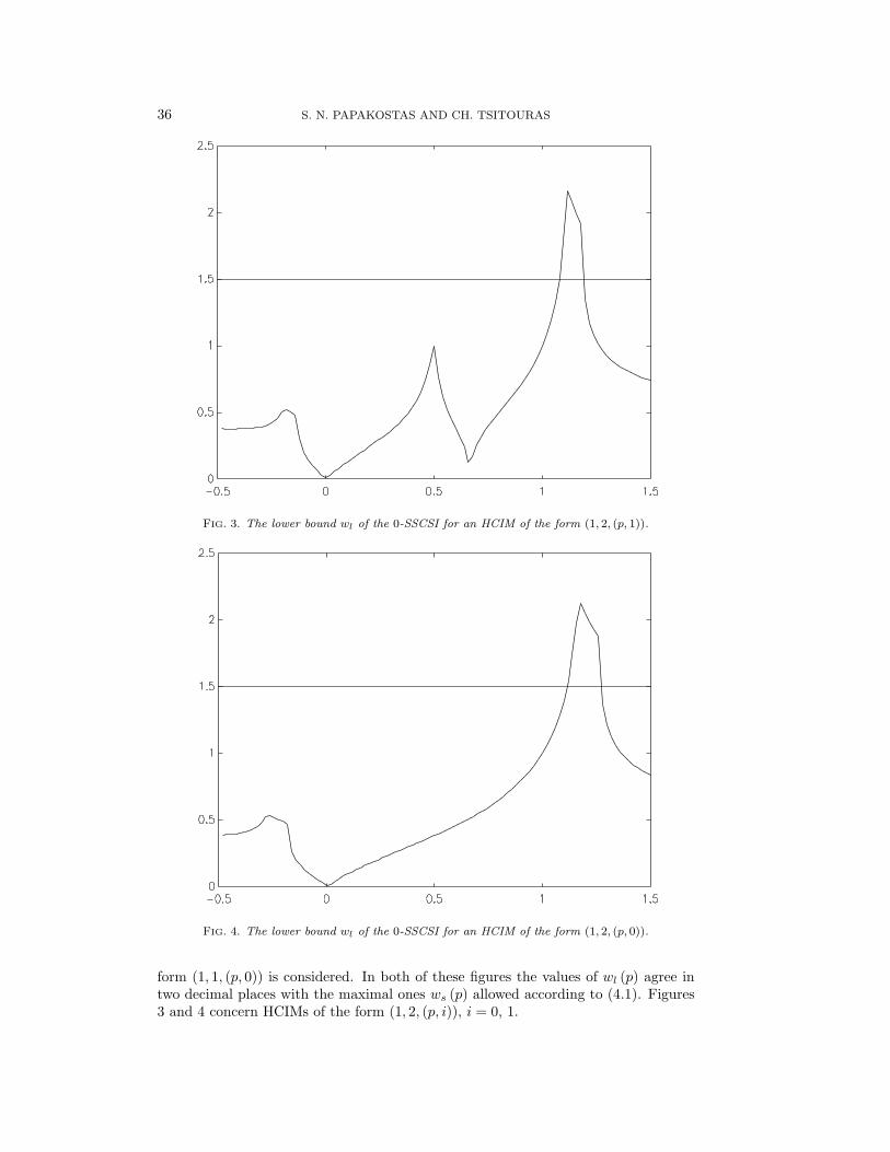
FIG. 3. The lower bound wl of the 0-SSCSI for an HCIM of the form (1, 2, (p, 1)).
FIG. 4. The lower bound wl of the 0-SSCSI for an HCIM of the form (1, 2, (p, 0)).
form (1, 1, (p, 0)) is considered. In both of these figures the values of wl (p) agree intwo decimal places with the maximal ones ws (p) allowed according to (4.1). Figures3 and 4 concern HCIMs of the form (1, 2, (p, i)), i = 0, 1.

HIGHLY CONTINUOUS INTERPOLANTS FOR ODE SOLVERS 37
FIG. 5. The continuous line represents the contour plot for wl = 1.5 of the 0-SSCSI for anHCIM of the form (1, 2, (p1, 1) , (p2, 1)). The dashed line concerns the same plot when the Calvo etal. norm is used.
FIG. 6. Contour plot for wl = 1.5 of the 0-SSCSI for an HCIM of the form (1, 2, (p1, 0) , (p2, 0)).
Figures 5, 6, and 7 correspond to HCIMs of the forms (1, 2, (p1, i) , (p2, j)), i,j = 0, 1. The contour plots presented in these figures are drawn for a safe value wlof the relevant 0-SSCSIs being equal to 1.5. Figures 8, 9, and 10 are the respective

38 S. N. PAPAKOSTAS AND CH. TSITOURAS
FIG. 7. Contour plot for wl = 1.5 of the 0-SSCSI for an HCIM of the form (1, 2, (p1, 0) , (p2, 1)).
FIG. 8. Contour plot for wl = 1.5 of the 0-SSCSI for an HCIM of the form (1, 3, (p1, 1) , (p2, 1)).
plots for HCIMs of the form (1, 3, (p1, i) , (p2, j)), i, j = 0, 1. Most interesting fromthe point of view of a practical implementation are those cases when the off-steppoints correspond to derivative data, as it is usually easier to find pointwise high-

HIGHLY CONTINUOUS INTERPOLANTS FOR ODE SOLVERS 39
FIG. 9. Contour plot for wl = 1.5 of the 0-SSCSI for an HCIM of the form (1, 3, (p1, 0) , (p2, 0)).
FIG. 10. Contour plot for wl = 1.5 of the 0-SSCSI for an HCIM of the form (1, 3, (p1, 0) , (p2, 1)).
order approximations of the derivatives than of the solution itself. (Actually thislowers by one the order of the system of the order conditions that must be solved.)

40 S. N. PAPAKOSTAS AND CH. TSITOURAS
FIG. 11. Contour plot for wl = 1.5 of the 0-SSCSI for an HCIM of the form (1, 3, (p, 1)).
Using (4.1) it may be seen that for HCIMs of the forms (1, 3, (p, i)), (1, 4, (p, i))when i = 0, 1 there exist no values of p which may yield possible SSCSIs for thesemethods (see Figures 11 and 12). A three-dimensional picture of wl for the case(1, 2, (p1, 1) , (p2, 1)) is presented in Figure 13.
The contour plots of all these figures show that many candidate HCIMs possessadequate stability characteristics and consequently might have good prospects of find-ing a practical implementation. A first attempt of assessment toward this directionis carried out in section 6.
5. Local truncation error considerations. Although the (zero) stability be-havior of the HCIMs introduced here depends on the ratios of successive integrationsteps, their LTE does not. Consider an HCIM of the form (1, k, (p1, δ1) , . . . , (pλ, δλ))applied on an effective s-stage RK pair, characterized by the triple A ∈ Rs×s, bT ,c ∈ Rs. In this section we will analyze the LTE for the case when all additional pointsused for the construction of the HCIM are based only on approximations of the solu-tion or its derivative provided by the original RK method as stated in Theorem 2.1.
Let the scaled (discrete) RK methods corresponding to the points (pi, δi), i =1,. . ., λ be described by the triples
A(i) =A 0
A(1,i) A(2,i) , b(i),
(cT ,(c(i))T)T
,
where
A =
0 0 · · · 0 00 a11 · · · a1s 0...
......
...0 as1 · · · ass 00 b1 · · · bs 0
,

HIGHLY CONTINUOUS INTERPOLANTS FOR ODE SOLVERS 41
FIG. 12. Contour plot for wl = 1.5 of the 0-SSCSI for an HCIM of the form (1, 4, (p, 1)). Thedotted line represents the upper bound for w, characterized by ws.
p1
p2
wl
FIG. 13. Three-dimensional picture of wl of the 0-SSCSI for an HCIM of the form(1, 2, (p1, 1) , (p2, 1)).

42 S. N. PAPAKOSTAS AND CH. TSITOURAS
c = A · e =(0, cT , 1
)T,
with
e ={1, . . . , 1}︸ ︷︷ ︸s+2
T
and the column dimensions of A(1,i) being identical to the dimension of c(i). Thisformulation is necessary if we want to use an original implicit RK method or if someof the stages of the scaled RK methods are computed implicitly. We also set di =dim
(c(i)). The parameters in
(A(1,i), A(2,i)
), b(i), c(i) (i = 1,. . ., λ) characterize the
extra function evaluations needed to describe the λ off-step approximations at thepoints (pi, δi) incorporated on the relevant HCIM.
Next we shall need to transform (2.1) in the compact form of an extended RKmethod. To this end let lij (t) be the generalized Lagrange polynomials of (2.1). Wedefine
A =
∣∣∣∣∣∣∣∣∣∣∣
AA(1,1) A(2,1) 0A(1,2) 0 A(2,2)
......
. . . . . .A(1,λ) 0 · · · 0 A(2,λ)
∣∣∣∣∣∣∣∣∣∣∣,
and we build up b (t) in the following way:
b (t) = (l0,1 (t) +λ∑i=1
lpi,δi (t) b(i)1 ,
l1,0 (t) b1 +λ∑i=1
lpi,δi (t) b(i)2 , . . . , l1,0 (t) bs +λ∑i=1
lpi,δi (t) b(i)s+1,
l1,1 (t) +λ∑i=1
lpi,δi (t) b(i)s+2,
lp1,δ1 (t) b(1)s+3, . . . , lp1,δ1 (t) b(1)
s+2+d1,
...lpλ,δλ (t) b(λ)
s+3, . . . , lpλ,δλ (t) b(λ)s+2+dλ).
If
c =(cT ,(c(1))T
, . . . ,(c(λ)
)T)T,
then the coefficients in the triple A, b (t), c together with l0,i (t), i = 2,. . ., κ + 1characterize completely the HCIM under consideration, if it is to be considered asa (κ+ 1)fold method propagating both the continuous solution and its higher orderderivatives at xn+1 (which are obtained by suitable differentiation).
The following theorem presents in a comprehensive way the order conditions ofthe HCIMs presented in section 2 in the context of the set of rooted trees T . Werecall that an RK method is of algebraic order p if and only if
X (τ) = 0 ∀τ ∈ Ti for i = 1 (1) p,

HIGHLY CONTINUOUS INTERPOLANTS FOR ODE SOLVERS 43
where Ti is the set of ith-order (rooted) trees and
X (τ) =1
σ (τ)
(Φ (τ)− 1
γ (τ)
).
σ, γ are integral functions of τ (symmetry and density function, respectively, in theterminology introduced by Butcher [1]), and Φ is a certain composition of A, b, c.
THEOREM 5.1. The LTE coefficients of an HCIM which is based on y, hy′ approx-imations on λ off-step points, applied to a RK method, are given by the expressions
1σ (τ)
(Φ(τ ; A, b, c
)−tρ(τ) −
∑λi=1 δρ(τ),iρ (τ)! l0,i (t)
γ (τ)
), τ ∈ T ,
where ρ (τ) is the order of tree τ . In this particular instance δij is the Kronecker delta.The expressions concerning the LTE of the higher order derivative approximations ofthe solution are obtained by differentiating suitably the above expression with respectto t.
Proof. Making use of the formulation developed immediately before this theorem,since l0,0 (t) = 1, equation (2.1) may be written as
y (t)− yn =κ∑i=2
l0,i (t)hiy(i)n + h
s∑i=1
bi (t) fn,i,(5.1)
where the fn,i correspond to the function evaluations (stages) needed for calculatingthe off-step approximations of the solution and/or its derivative. If we assume yto be infinitely differentiable, according to a generalization of a result (see [1], [15])concerning the LTE coefficients of a discrete RK method to the continuous case, it isfound that
y(i)n =
∑( τ∈Tρ(τ)=i)
α (τ)F (τ ; f ; yn) ,(5.2)
where
α (τ) =ρ (τ)!
σ (τ) γ (τ)
and F (τ ; f ; yn) are the so-called elementary differentials. Furthermore, from a formalTaylor series expansion we may find
y (t)− yn =∞∑i=1
(t h)i
i!y(i)n =
∞∑i=1
(t h)i
i!
∑( τ∈Tρ(τ)=i)
α (τ)F (τ ; f ; yn) .(5.3)
The second term in the right-hand side of (5.1) may be expanded in the infinite series
h
s∑i=1
bi (t) fn,i = h∞∑i=1
hi−1
i!
∑( τ∈Tρ(τ)=i)
α (τ) γ (τ) Φ(τ ; A, b, c
)F (τ ; f ; yn) .(5.4)
Substituting (5.2), (5.3), (5.4) in (5.1) we may estimate the desired LTEexpressions.

44 S. N. PAPAKOSTAS AND CH. TSITOURAS
6. Selection and numerical performance of some C 2 and C 3 interpola-tory schemes. The results of section 4 assure us that the construction of HCIMs forRK pairs, as long as the 0-SSCSI characteristics are concerned, is quite feasible. Oncethis part of the problem is solved, it has been solved for any RK pair of a specificorder (in this respect, Figures 1 to 12 cover all interesting cases). The other part ofthe problem is that of finding suitable values for the additional off-step points, whichwill enable the construction of particular highly continuous interpolants optimizedwith respect to their LTE coefficients for specific RK pairs.
As the HCIMs introduced here are mainly for illustrative and comparison pur-poses, we shall present numerical results concerning only RK pairs of orders five andsix. This is also due to the fact that the only reliable classical (one-step) interpolantsthat have appeared in the literature are only of orders five and six, corresponding topairs of the same orders, respectively. As of the time of this writing, the authors arenot aware of the existence of reliable RK interpolants of seventh or higher order.
The first of the HCIMs to be compared here is of the form (1, 1, (p, 1)), andit thus gives a C2, fifth-order interpolant for any fifth-order RK pair. Specifically,this method, when applied to the pairs FE5(4)#2 [13] and DP5(4) [9], results in themethods denoted NEW1 and NEW2, respectively, construction of which requires onlyone additional function evaluation. This is because for these pairs, with effectivelyone additional function evaluation only, a fifth-order approximation of the first-orderderivative of the solution may be obtained at any point inside or outside the integrationinterval. Both methods NEW1 and NEW2 are based on the selection p = 0.4, whichoffers an infinite 0-SSCSI.
A C3 HCIM may be obtained for the pair used in the code DVERK, VE6(5)(Verner [33]; Hull, Enright, and Jackson [22]), which again effectively uses only oneadditional function evaluation to the eight already used by this pair. For the pairVE6(5), a fifth-order, cost-free pointwise approximation of the solution at any point(say p) may be found. Thus with one additional function evaluation, a sixth-orderapproximation of the first-order derivative of the solution may be obtained at thesame point p. For the selection p = 1.12 the resulting pair is denoted as NEW3.
We must remark that the selection of the off-step points in all of the above HCIMswas motivated exclusively by stability considerations (maximization of the relevant0-SSCSIs), and no compromise with respect to the magnitude of the local truncationerrors of the resulting continuous methods was made. Hence, other selections mightlead to even more efficient methods.
The continuous extensions of the pairs we chose to test the new methods areamong the most reliable and competitive that have appeared in the literature. All ofthem are one step in their nature. The first of these is the fifth-order interpolant for thepair FE5(4)#2, constructed by Calvo, Montijano, and Randez [5], which effectivelyuses two additional function evaluations. The second interpolant is built up on theDP5(4) pair, and it has been proposed by the same authors [4], [5]. It has the sameorder and cost in function evaluations as the first.
For illustrative reasons, we decided to include also in our tests a continuous fifth-order pair due to Owren and Zennaro [25]. The approach followed by these authors issomewhat different than that usually adopted, since their method is not based on anypreviously known pair, but rather it has been constructed with the sole purpose ofproviding a continuous fifth-order pair with the minimal cost in function evaluations.
The fourth interpolant used in our comparisons concerns the pair used in DVERK,and it is owed to Enright, Jackson, Nørsett, and Thomsen [11]. It is a sixth-orderinterpolant, and its cost is effectively three additional function evaluations.

HIGHLY CONTINUOUS INTERPOLANTS FOR ODE SOLVERS 45
TABLE 1Efficiency gains of the Calvo et al. fifth-order interpolant for the pair FE5(4) with respect to
NEW1 (fifth-order C2), over nine problems of DETEST.
A1 A2 A3 A4 D1 D2 D3 D4 D50 13 11 11 11−1 13 12 11 11 11−2 11 14 12 12 12 12
log −3 8 12 12 14 13 12 13 13global −4 14 14 12 12 14 14 13 14 14error −5 14 15 12 12 14 14 14 14
−6 13 15 13 13 14 14−7 12 14 14−8 11 14 15−9 10 14−10
12.7% 12 13 12 13 14 13 13 12 12
TABLE 2Efficiency gains of the Calvo et al. fifth-order interpolant for DP5(4) with respect to NEW2
(fifth-order, C2) over nine problems of DETEST.
A1 A2 A3 A4 D1 D2 D3 D4 D50 12 14−1 13 10 11 2 15−2 14 10 11 3 17
log −3 15 11 15 14 10 12 5 18global −4 0 15 11 14 14 9 12 9 23error −5 2 15 11 13 14 4 14 12
−6 5 15 11 13 14 1 14−7 8 15 12 13−8 10 15 13 13−9 14 15−10
11.3% 7 15 12 13 14 7 12 5 17
TABLE 3Efficiency gains of the Owren–Zennaro seven-stage, fifth-order interpolant with respect to
NEW2, over nine problems of DETEST.
A1 A2 A3 A4 D1 D2 D3 D4 D50−1 −1 −2−2 −6 −17 1 −4 1
log −3 −3 −4 4 −8 5global −4 −13 26 14 6 9 3 −12 7error −5 −8 −17 36 −2 20 12 0 −13
−6 −1 −8 40 10 34 14 −5−7 3 5 56 15−8 10 12 20−9 16 23−107.2% 1 3 40 12 10 3 1 −8 3
Tables 1, 2, 3, and 4 contain the efficiency gain results (in the spirit of Enrightand Pryce [12]) when testing all of the above methods in pairs on the nine DETESTproblems [21] with a known analytical solution and for tolerances 10−3, 10−4,. . ., 10−9.A detailed explanation of how these tables were obtained may be found in Sharp [29]or in Papakostas, Tsitouras, and Papageorgiou [27].

46 S. N. PAPAKOSTAS AND CH. TSITOURAS
TABLE 4Efficiency gains of the Enright et al. fifth-order interpolant for the pair VE6(5) of DVERK with
respect to NEW3 (fifth-order C3), over nine problems of DETEST.
A1 A2 A3 A4 D1 D2 D3 D4 D50 6 8−1 19 13 12 10 9−2 9 8 11 9 9
log −3 9 6 −4 3 11 9 10global −4 16 10 9 5 −13 2 10 9error −5 15 10 9 5 −22 −7 9
−6 15 10 9 3 8−7 18 11 9 3−8 19 9 2−9 19−10 227.8% 18 10 9 4 −2 4 10 8 9
In the tables unity represents 1 percent. Numbers have been rounded to thenearest integer. Positive numbers mean that the second of the two methods is superior.The final row gives the mean value of efficiency gain for each tolerance and problem.The final row’s first number is the average efficiency gain over all problems. Emptyplaces in the tables are due to the unavailability of data for the respective tolerances.
The percentage numbers observed from these tables show that in general thenew HCIMs proposed here seem to offer interpolants that are more efficient thanthe existing classical one-step interpolatory technique. Since no particular truncationerror minimization took place when choosing the off-step points, we may attribute thisperformance exclusively to the lower cost in function evaluations (a potential benefitoffered by the new method).
When taking into account the possible reduction of the cost in necessary functionevaluations and the simplified approach inherent in the new interpolatory techniquewhen applied to high-order one-step methods, it is very probable that this methodmight offer good prospects for the construction of interpolants of an even higher degreeas well. The authors intend to study in the future some other aspects of this problem.
REFERENCES
[1] J. C. BUTCHER, The Numerical Analysis of Ordinary Differential Equations, John Wiley andSons, New York, Chichester, 1987.
[2] M. CALVO, T. GRANDE, AND R. D. GRIGORIEFF, On the zero stability of the variable ordervariable stepsize BDF-formulas, Numer. Math., 57 (1990), pp. 39–50.
[3] M. CALVO, F. LISBONA, AND J. MONTIJANO, On the stability of variable-stepsize NordsieckBDF methods, SIAM J. Numer. Anal., 24 (1987), pp. 844–854.
[4] M. CALVO, J. I. MONTIJANO, AND L. RANDEZ, A fifth order interpolant for the Dormand andPrince Runge-Kutta method, J. Comput. Appl. Math., 29 (1990), pp. 91–100.
[5] M. CALVO, J. I. MONTIJANO, AND L. RANDEZ, New continuous extensions for fifth orderRunge-Kutta formulas, Rev. Acad. Ciencias Zaragoza, 45 (1990), pp. 69–81.
[6] M. CALVO, J. I. MONTIJANO, AND L. RANDEZ, A new embedded pair of Runge-Kutta formulasof order 5 and 6, Comput. Math. Appl., 20 (1990), pp. 15–24.
[7] A. R. CURTIS, High order explicit Runge-Kutta formulae, their uses and their limitations, J.Inst. Math. Appl., 16 (1975), pp. 35–55.
[8] P. J. DAVIS, Interpolation and approximation, Dover, New York, 1975.[9] J. R. DORMAND AND P. J. PRINCE, A family of embedded Runge-Kutta formulae, J. Comput.
Appl. Math., 6 (1980), pp. 19–26.[10] J. R. DORMAND AND P. J. PRINCE, Runge-Kutta-Nystrom triples, Comp. Math. Appl., 13
(1987), pp. 937–949.

HIGHLY CONTINUOUS INTERPOLANTS FOR ODE SOLVERS 47
[11] W. H. ENRIGHT, K. R. JACKSON, S. P. NØRSETT, AND P. J. THOMSEN, Interpolants forRunge-Kutta formulas, ACM Trans. Math. Software, 12 (1986), pp. 193–218.
[12] W. H. ENRIGHT AND J. D. PRYCE, Two FORTRAN packages for assessing initial value meth-ods, ACM Trans. Math. Software, 13 (1987), pp. 1–27.
[13] E. FEHLBERG, Low Order Classical Runge-Kutta Formulas with Stepsize Control and TheirApplication to Some Heat-Transfer Problems, Technical report TR R–315, NASA, GeorgeMarshal Space Flight Center, Huntsville, AL, 1969.
[14] R. D. GRIGORIEFF, Stability of multistep methods on variable grids, Numer. Math., 42 (1983),pp. 359–377.
[15] E. HAIRER, S. P. NØRSETT, AND G. WANNER, Solving Ordinary Differential Equations I,Springer-Verlag, Berlin, New York, 1987.
[16] E. HAIRER AND G. WANNER, Multistep-multistage-multiderivative methods for ordinary dif-ferential equations, Computing, 11 (1973), pp. 287–303.
[17] H. M. HEBSAKER, Neue Runge-Kutta-Fehlberg-Verfahren fur Differentialgleichungs-Systemen-ter Ordnung, PhD thesis, Siegen, 1980.
[18] H. M. HEBSAKER, Conditions for the coefficients of Runge-Kutta methods for systems of nthorder differential equations, J. Comput. Appl. Math., 8 (1982), pp. 3–14.
[19] D. J. HIGHAM, Highly continuous Runge-Kutta interpolants, ACM Trans. Math. Software,17 (1991), pp. 368–386.
[20] M. K. HORN, Fourth and fifth order scaled Runge-Kutta algorithms for treating dense output,SIAM J. Numer. Anal., 20 (1983), pp. 558–568.
[21] T. E. HULL, W. H. ENRIGHT, B. M. FELLEN, AND A. E. SEDGWICK, Comparing numericalmethods for ordinary differential equations, SIAM J. Numer. Anal., 9 (1972), pp. 603–637.
[22] T. E. HULL, W. H. ENRIGHT, AND K. R. JACKSON, Users Guide for DVERK—a Subroutinefor Solving Non-Stiff ODEs, TR 100, Dept. of Comp. Sci., Univ. of Toronto, Toronto,Canada, 1976.
[23] A. NORDSIECK, Automatic numerical integration of ordinary differential equations, Math.Comp., 16 (1963), pp. 22–49.
[24] B. OWREN AND M. ZENNARO, Order barriers for continuous explicit Runge-Kutta methods,Math. Comp., 56 (1991), pp. 645–661.
[25] B. OWREN AND M. ZENNARO, Derivation of efficient, continuous, explicit Runge-Kutta meth-ods, SIAM J. Sci. Statist. Comput., 13 (1992), pp. 1488–1501.
[26] G. PAPAGEORGIOU AND C. TSITOURAS, Scaled Runge-Kutta-Nystrom methods for the secondorder differential equation y′′ = f (x, y), Internat. J. Computer Math., 28 (1989), pp. 139–150.
[27] S. N. PAPAKOSTAS, C. TSITOURAS, AND G. PAPAGEORGIOU, A general family of explicitRunge-Kutta pairs of orders 6(5), SIAM J. Numer. Anal., 33 (1996), pp. 917–936.
[28] L. F. SHAMPINE, Interpolation for Runge-Kutta methods, SIAM J. Numer. Anal., 22 (1985),pp. 1014–1027.
[29] P. SHARP, Numerical comparisons of some explicit runge-Kutta pairs of orders 4 through 8,ACM Trans. Math. Software, 17 (1991), pp. 387–409.
[30] R. D. SKEEL AND W. JACKSON, The stability of variable-stepsize Nordsieck methods, SIAM J.Numer. Anal., 20 (1983), pp. 840–853.
[31] C. TSITOURAS AND G. PAPAGEORGIOU, New interpolants for Runge-Kutta algorithms usingsecond derivatives, Internat. J. Computer Math., 31 (1989), pp. 105–113.
[32] C. TSITOURAS AND G. PAPAGEORGIOU, Runge-Kutta interpolants based on values from twosuccessive integration steps, Computing, 43 (1990), pp. 255–266.
[33] J. H. VERNER, Explicit Runge-Kutta methods with estimates of the local truncation error,SIAM J. Numer. Anal., 15 (1978), pp. 772–790.
[34] J. H. VERNER, Differentiable interpolants for high-order Runge-Kutta methhods, SIAM J.Numer. Anal., 30 (1993), pp. 1446–1466.
[35] R. ZURMUHL, Runge-Kutta-verfahren zur numerischen integration von differentialgleichungenn-ter ordnung, Z. Angew. Math. Mech., 28 (1948), pp. 173–182.