high-resolution radar based object classiﬁcation for

High-Resolution Radar Based Object Classificationfor Automotive Applications

Ganesh NageswaranDepartment of Mechanical and Process Engineering

Technical University of KaiserslauternKaiserslautern, Germany

[email protected]

Abstract—This paper presents a method for classifying trafficparticipants based on high-resolution automotive radar sensorsfor autonomous driving applications. The major classes of trafficparticipants addressed in this work are pedestrians, bicyclistsand passenger cars. The preprocessed radar detections arefirst segmented into distinct clusters using density-based spatialclustering of applications with noise (DBSCAN) algorithm. Eachcluster of detections would typically have different propertiesbased on the respective characteristics of the object that theyoriginated from. Therefore, sixteen distinct features based onradar detections, that are suitable for separating pedestrians,bicyclists and passenger car categories are selected and extractedfor each of the cluster. A support vector machine (SVM) classifieris constructed, trained and parametrised for distinguishing theroad users based on the extracted features. Experiments are con-ducted to analyse the classification performance of the proposedmethod on real data.

Index Terms—radar, clustering, feature extraction, object clas-sification, machine learning, autonomous driving

I. INTRODUCTION

High-resolution radars in the frequency range 77-79 GHzare recently developed for usage in many automotive applica-tions. With an increased resolution, multiple reflection pointsare detected from an extended object. Therefore the usualassumption of an object as point target is not valid any moreand the spatial extent of the object also needs to be considered.Moreover, every object has it’s own distinct features. Forexample, a pedestrian walks with a velocity which is verydistinct from the velocity of a car, or the dimensions ofa cyclist are smaller compared to a truck. Extracting suchfeatures out of measurements originating from an object wouldhelp to classify that object.

Vast number of methods have already been proposed fordetecting and classifying objects based on range sensors.In a method proposed in [1], [2], objects can be detectedand classified based on shape models. Classification basedon measurement characteristics and motion analysis is pre-sented in [3], [4]. Distance based clustering of detections andfitting one of the pre-defined shape models to the clusterto infer the object type is proposed in [5]. [6] proposes

This work was carried out by the author during his tenure as ScientificEmployee at the Department of Mechanical and Process Engineering atTechnical University Kaiserslautern, in cooperation with the company Knorr-Bremse System for Commercial Vehicles Private Limited in Schwieberdingen.

a method of joint object tracking and classification basedon laser scanner, where the defined object classes are 0-axis, 1-axis or 2-axes objects. A Markov chain based ondifferent observation positions of the object is constructed.The transition probabilities are defined based on the objectmanuever and the corresponding observation of the sensor.In [7], a method for segmentation of measurements fromlaser scanner and consecutive feature extraction from thesesegments is proposed. The extracted features are then usedfor training different machine learning based classifiers todetect pedestrians. As the measurement resolution of radarsensors in automotive domain have significantly improved inthe recent years, we propose an hybrid approach in this work,which combines the clustering algorithms typically applied forlaser scanner sensors, with the machine learning techniques forclassifying road users.

The proposed solution constitutes a sequence of steps whichcan be abstractly put as segmentation, feature extraction andclassification. After an initial pre-processing, density basedspatial clustering of applications with noise (DBSCAN) al-gorithm [8] is used for segmenting high-resolution radardetections into distinct clusters. From the object tracking pointof view, each cluster is fitted with pre-defined geometric shapeand a reference point is chosen accordingly, which couldbe used as a reference measurement point of the object fortracking. Apart from the geometric shape, sixteen pre-definedfeatures that could explain the potential characteristics of theunderlying object are extracted for each of the cluster. Asupport vector machine (SVM) classifier is constructed andtrained with the help of these object features, which can thenbe used in real-time for classifying pedestrians, bicyclists andpassenger cars.

The remainder of this article is organised as follows. SectionII presents the methods for segmentation of the radar data,which involves the pre-processing and data clustering steps.Different geometric and characteristic features that could behelpful in distinguishing the road users and how they canbe extracted from radar data are presented in section III.Classification based on SVM classifier and the results arepresented in section IV and section V. A short summary withremarks is given in section VI.

II. SEGMENTATION OF RADAR DATA

A. Data pre-processing

Radar measures the range, azimuth and Doppler velocity,which are extracted for each measurement point dependingon the underlying measurement principle, for example withfrequency modulated continuous wave (FMCW) detectionmethod. Unlike a point target, multiple detections can originatefrom an extended object. Therefore the segmentation algorithmtries to sort out the detection points as unique groups. Ideallyeach group or cluster should contain all the detections thatbelong to a single extended object. A typical problem withradar sensor is the so called double reflection, where theelectro-magnetic waves from the radar reflected by the objectsurface is strong enough to be reflected back again by the radarmounting or the ego-vehicle surface. If the amplitude is highenough, these double reflections would create a peak in theFast Fourier Transform (FFT), thereby creating false positiveobjects. Therefore, some pre-preprocessing of the detectionsis required in order to avoid these false positive objects. Thedouble reflections from the same object need to filtered out,before grouping them. Although the measured azimuth in thecase of a double reflection would be nearly the same, the rangeand Doppler velocity would have values that are in multiplesof two or more.

θdouble ≈ θsinglerdouble = 2 · rsinglerdouble = 2 · rsingle

(1)

Additionally, also the detection points which have an unreal-istic Doppler velocity values are filtered out before clustering.These are typically clutter measurements which is prevalentwith radar sensors.

B. Clustering of radar detections

After the pre-processing of the raw detections, the remainingdetection points can be understood as belonging to the objectsin the environment, either pedestrians, bicyclists, vehiclesor other infrastructures. The basic concept of the DBSCANalgorithm is that, any point in a cluster should contain a certainnumber of other points within a particular defined radius.Which means, a group of points make a cluster if their densityis higher than particular threshold. The distance between twopoints p and q can basically be described by any distancefunction dist(p, q). Euclidean distance function is used in thiswork. Basic definitions are made in [8] which defines Eps,MinPts, core point and border points.

Eps is defined as the threshold radius, which representsthe neighbourhood of a point. The Eps-neighbourhood of apoint p denoted as NEps(p) is defined by NEps(p) = [q ∈D|dist(p, q) ≤ Eps]. Further as illustrated in the Figure 1,the point p is a core point, if it has at least MinPts numberof points in it’s neighbourhood and also those neighbouringpoints are directly density-reachable from p. If there is apoint q1 within the Eps-neighbourhood of p but do not haveMinPts number of points that are directly density-reachable

from it, then q1 would be a border point. q1 is directly density-reachable from p but not the other way, as directly density-reachable is defined to be symmetric only for the connectionsbetween the core points. Considering another point r in theFigure 1, q1 is said to be density-reachable from r through thepath of points p1, . . . pn, with p1 = r, pn = q1, and rest of thepoints pi+1 also being core points. The definition of density-connected connects two border points q2 and q1 through thepoint r as they are both density-reachable from the core pointr. Now starting from point p, including all the core pointsthat directly density-reachable from p and the border points q1and q2 that are density-connected between them and density-reachable from p form a cluster.

q1

p

r

n

q2

Fig. 1: Illustration of the DBSCAN algorithm

Clustering parameters selection: The parameters Eps andMinPts usually could to be selected based on the applicationat hand. [8] proposes k-dist graph method for selection ofthese parameters, from the thinnest cluster of points. However,the suggestion is intended mainly for unknown applicationsituations. For our application case, the objects of interestin the environment are more or less known a-priori, whichof all the pedestrian category has the least spatial extension.Another factor in selecting the parameter is that, the densityand number of points reflected from an object depends stronglyon the position of the object with respect to sensor. When theobject is closer to the radar sensor it generates more reflectionpoints, whereas when it is detected at the farthest position inthe FoV, only a single point could be generated. From manymeasurements it was empirically observed that all the objectclasses generated as less as one detection point at the edge ofFoV. At closer positions to the sensor, pedestrians generatedup to six detections, bicyclists up to seven detection points anda passenger car up to twenty detection points. Intuitively, formany low speed use cases of autonomous driving, the area veryclose to the ego-vehicle is of high relevance and the clusteringin that area needs to be reliable, than at a higher distance.

III. FEATURE EXTRACTION

The ideal output of the above defined clustering are welldefined distinct clusters, each representing a distinct object.Further in the feature extraction step, distinct object hy-potheses are searched and extracted for each segment. Onan abstract level, the hypotheses can be divided into twocategories, namely the shape or extension of the object and

the distinct characteristic features of the object. Pedestriansare considered in this work to have a circular extension,bicyclists stick extension and other vehicles as rectangularboxes. Therefore three shape model assumptions are madewith O-shape representing pedestrians, I-shape representingone side of vehicle and bicyclist and L-shape representing twosides of vehicle. Similar kind of approach is used in many ofthe earlier works such as [5]. The parameters of the shapefeature are then extracted by fitting the detection points ineach cluster to one of the above defined models sequentially.

A. Fitting a geometric shape

Before beginning with the actual shape fitting, an idea onwhat kind of shapes should be tried for each cluster can beobtained by checking the 2-dimensional spatial spread of thedetections in the cluster. In other words, if the detectionsare spread along both the longitudinal and lateral axes, andthere are many detections available in the cluster, the clusterwould supposedly have a larger extension. If the spread isonly along one axis, it would potentially be a line type. Amethod for applying such a pre-selection is proposed in [5].Principal component analysis (PCA) is applied on each of theclusters and the corresponding eigenvalues of the covariancematrix are calculated. If the ratio of the eigenvalues is greaterthan a certain threshold, it would mean that the spread isdominated by one of the axes and therefore only I-shape istried further for that cluster. In the other case, when the ratioof the eigenvalues is lesser than the pre-defined threshold, thespread is potentially along both the axes and therefore L-shapeis tried to be fit. Additionally, if the number of detection pointsin the cluster is less than Nmin, the cluster is assumed to haveO-shape.

There are many methods and algorithms available from thefield of robotics for extracting lines from a set of points. Someimportant methods are summarized in [9]. If the model pre-selection denotes that a segment must be tested for both L-shape and I-shape, iterative end point fit (IEPF) algorithm isfirst applied on that segment. The algorithm is also known inliterature under the variants Ramer-Douglas-Peucker (RDP)algorithm or split-and-merge algorithm. The basic idea is tofit a line with first and the last point of the segment and finda point which has the maximum orthogonal distance to thisline. This point intuitively is the corner point and the set issplit into two individual set of points at this point. Lines arethen fit individually to these sets of points. Now we are leftonly with the segments that need to be looked for I-shape.

Hough-Transform introduced by Richard Duda and PeterHart is a widely used method in the field of computer visionfor extracting line segments out of images. The key idea is torepresent a line in it’s Hesse normal form

r = x cos θ + y sin θ (2)

where r is the perpendicular distance from origin to the lineand θ the angle made by the line with x-axis. The line isrepresented in the above normal form instead of general formy = mx+b because in case of vertical line the slope parameter

(a) L-shape (b) I-shape (c) O-shape

Fig. 2: Considered geometric shapes for detection clusters. Theblack color cross represents the corresponding reference point(RP) chosen for the fitted shape

would lead to singularity. Whereas a vertical line in normalform can be represented with θ = 90°and r equal to the x-axis intercept. The parameter space or Hough space is givenby (r, θ). Generally speaking, any number of lines can bedrawn through a given point in xy-plane. This would meana sinusoidal curve for each point on the Hough-space withvarying θ and r. Such sinusoidal segment is constructed forall the points in the cluster. Then the value of r′ and θ′ inthe Hough-space, where the sinusoidal curves of all pointsintersect would give the line in the xy-plane, which passesthrough all those points or in other words a line which fits thepoints in the cluster.

After fitting a line to the points, the clusters which showeda possibility of L-shape are checked for line segments whichare almost perpendicular to each other. In that case, the linesegments are merged to fit the L-shape and a rectangularbounding box covering the nearest and farthest coordinate inthe cluster is overlayed on the cluster as represented in Figure2 to represent it’s shape hypothesis. The orientation of thecluster is calculated by PCA. The covariance and eigenvectorsare calculated similar to the method as described previouslyfor pre-selection. The orientation of the cluster is then givenby the direction of the eigenvector v1 with highest eigenvalueλ1

ψL = tan−1(v1(y)

v1(x)

)(3)

In order to calculate the four corner points of the boundingbox, all the points in the cluster are first rotated by theorientation angle, so that the eigenvector v1 is parallel to thex-axis. After rotation, the maximum and minimum values ofthe x and y coordinates in the cluster represent the lengthand width of the bounding box. The coordinates of the cornerpoints (p1, p2, p3, p4) representing the bounding box are finallycalculated by again rotating the points of the cluster by it’sorientation angle in the opposite direction. The corner pointof the bounding box closest to the sensor can be then chosenas reference measurement point for the cluster, which could beused by the tracking algorithms. If there are no perpendicularline segments that are to be merged, the cluster is then denotedwith I-shape hypothesis and the middle point of the line ischosen as the reference point. The orientation of the I-shapeis then same as the estimated angle θ′. As stated before, ifthere are not enough points for both of the L-shape and I-

Pedestrian Bicyclist Car

0

1

2

3

F14:DopplerVariance


10

20

30

F1:NumOfPoints


5

10

15

F15:RangeWgdPower


0

200

400

F16:PowerDBvar

Pedestrian Bicyclist Car0

1

2

F6:BBLength


2

4

F7:BBWidth


5

10

15

F8:BBCircum


0

5

10

15F9:BBArea


500

1000F10:BBDensity


1

2

F2:Compactness


0

10

20

F3:Linearity


0

5

10F4:Circularity


2

4

F5:Radius


5

10

F11:BoundaryLength


0

5

10

F13:PolygonAreaPedestrian Bicyclist Car

0

0.5

1

1.5

F12:BoundaryRegularity

Fig. 3: Boxplot of all the features for each class

shape, the cluster is denoted with O-shape. In this case, theorientation is not known and set to zero, and the point can bechosen as reference measurement point.

B. Characteristic feature description

In addition to the geometric features, each cluster basi-cally contains other characteristics features as well, whichare representative of the actual object class that the clusterbelongs to. Methods for extraction of characteristic featuresfrom measurement clusters and how these features can be usedto classify objects has been previously studied in [10], [11]and [12], to name a few. In addition to the features describedin [10], basically meant for laser scanner, new radar specificfeatures are defined and extracted for each of the cluster inthis work. The features that are of interest for each cluster Cof radar detections are:• Number of points: denotes the total number of detection

points in that cluster

NumOfPoints = |Ci| (4)

• Standard deviation: The standard deviation of the posi-tion of points is given by

Compactness =

√1

n− 1

∑j

‖xj − x‖2 (5)

where x is the centroid of the cluster and xj the positionsof each point.

• Linearity: This feature denotes the residual sum ofsquares between the cluster points and a line fitted tothe cluster points [10]. Given the line parameters r

′and

θ′, linearity can be calculated as

Linearity =∑j

(xj cos(θ′) + yj sin θ′ − r′)2 (6)

• Circularity: The residual of sum of squares to a circlefitted for points in the cluster is denoted by this feature.If a circle of radius R and center (xc, yc) is fitted to the

points by least squares method, then the circularity of thecluster is given as in [10] by

Circularity =

n∑j=1

(R−

√(xc − xj)2 + (yc − yj)2

)2

(7)with (xj , yj) denoting the positions of detection pointsin Cartesian coordinates.

• Radius: Denotes the radius R of the circle fitted to thecluster for calculating circularity feature.

• Length of minimal bounding box: The length of a bound-ing box BBLength that would cover the points in thecluster is calculated as explained in section III-A. Forperfect line this value would be zero.

• Width of minimal bounding box: This feature representsthe width of the assumed bounding box BBWidth, againas calculated in section III-A.

• Circumference of assumed bounding box: Circumferenceof the bounding box

BBCircum = 2 · (BBLength+BBWidth) (8)

• Area of assumed bounding box: The area of the rectan-gular bounding box is calculated as

BBArea = BBLength ·BBWidth (9)

• Density of assumed bounding box: Density of the bound-ing box is the ratio of number of points in the cluster nto its area areaBB

BBDensity =NumOfPoints

BBArea(10)

• Length of the boundary: The length of the contour formedby connecting the points in a cluster is calculated by

BoundaryLength =∑j

d(pj , pj−1)

d(pj , pj−1) =√

(xj − xj−1)2 + (yj − yj−1)2

(11)

• Boundary regularity: The standard deviation of the dis-tances d(pj , pj−1) as in [10].

• Polygon Area: The area of the polygon fitted to the clusterof detection points.

• Doppler variance: This feature denotes the varianceof the Doppler velocity within a cluster. Due to themovement of the arms and legs, the Doppler variance ofthe pedestrian class is expected to be higher than otherclasses.

• Range weighted mean power: The amplitude of electro-magnetic wave reflected from metal surfaces, as in caseof vehicles, is expected to be higher than that of weakreflecting surfaces like pedestrian body. This feature istherefore used for representing the reflection characteris-tic of an object. However, the reflection power of objectsthat are in a closer range to the sensor is greater thanthat of the object at a higher range. In order to considerthis range dependency, a weight is given to the power

Fig. 4: Biplot of all the features projected onto first 3 PCs

of a reflection point in the cluster. The weight should beinversely proportional to the range

RangeWgdPower =

∑j

wjA(j)

n

where wj =1

rj

(12)

• Power variance: This feature represents the varianceof reflection power in a cluster and is denoted byPowerDBvar. Objects with regular reflecting surfaceslike passenger car is expected to have a lesser varianceof the reflected power through out it’s contour, whereasa bicycle for example can have a higher variance.

1) Dimensionality reduction: The relevance of all the fea-tures described above for class separation is usually not knownexplicitly. PCA is a widely used method in machine learningfield, to analyse the contribution of each feature to the classifi-cation problem and subsequently for dimension reduction. Thefeature vectors are projected onto a lower dimension with thehelp of the principal components (PC). The so called PCs arethe vectors that capture the highest variance of the data. Figure4 shows the bi-plot with corresponding data projected onto thefirst three PCs and also the coefficients representing the vari-ance contribution. As can be seen, the features BBDensityand PowerDBvar dominates the first two PCs and otherfeatures are entangled in the subsequent higher dimensionalPCs. The feature number of points NumOfPoints and thefeatures representing dimensions, area and density are highlycorrelated, pointing in similar direction in the bi-plot. A bi-plot illustrating the contribution of these features, neglectingthe BBDensity and PowerDBvar is given in Figure 5.

2) Remark: Many of the features like NumOfPointsare dependent on the actual position of the object withrespect to sensor. Consequently many features like circularity,radius, bounding box fit, area etc. are dependent on theNumOfPoints in the cluster. But at a higher distance fromsensor, as even a passenger car may only show same character-istic features as a pedestrian, considering these features in such

Fig. 5: Biplot of reduced features projected onto PCs

conditions would cause a bias in class separability. On solutionto overcome this would be to divide the overall classificationinto two sub-methods, considering the position dependabilityof the features. As the radar can measure the Doppler velocityof the object, it could be used as a fallback feature for thecases where the main classifier cannot give class probabilitiesbased on all the defined features. But in conditions where theobject moves with the same velocity as the ego-vehicle, thiswould again cause a higher misclassification. In most of theautonomous driving use cases, the detections of the sensorsare fed into tracking algorithms to build a stable object state.Therefore for the condition with NumOfPoints < 3, theclassification could be purely based on the estimated velocityof the tracked object. Moreover, the classification output couldactually be a fused result of the track velocity and the resultof the classifier, using some evidence based fusion techniquessuch as Dempster-Shafer method.

IV. CLASSIFICATION

Pedestrians and bicyclists are obviously very prevalent ur-ban environments, than in highways. Also most of the automo-tive grade short range radar sensors with high resolution areused for near range sensing applications such as turning assistor assisted parking. In such cases, object is expected to bein the sensor FoV for only a relatively shorter time interval.Which from the other point of view means that in order tohave many training samples, many hours of test data needs tobe logged for training the classifier. Support Vector Machine(SVM) is one of the classification methods that is least affectedby the training data sample size [13]. Therefore for objectclassification, SVM is used in this work. As mentioned inthe previous section, the validity of feature extraction dependshighly on the position of the object in the sensor’s FoV. Theazimuth separation for the classifier is empirically selected at−60°and +60°, based on many measurement observations.

A. SVM for classifying road users

Since it’s introduction in [14], SVM has been widely usedin vehicle environment perception applications like image

based detection of objects, vehicle maneuver prediction etc.SVM is a maximum margin classifier, which is able to derivea decision boundary between various classes in question.Basically the boundary is an hyperplane, calculated by map-ping the inputs to higher dimensional feature space. Moreformally the problem can be stated as, given a set of trainingdata {(x1, y1), . . . (xn, yn)} with xi ∈ X as input data andyi ∈ C = {−1, 1} the class labels, the SVM calculates adecision function F (x), which can then be used for predictingthe value yk for an input xk at the time k [15]. If the data inx are linearly separable, the decision boundary separating theclasses would be the optimal hyperplane in the input space X ,which is given by the decision function

F (x) =

N∑i=1

wi(xi) + b = 0 (13)

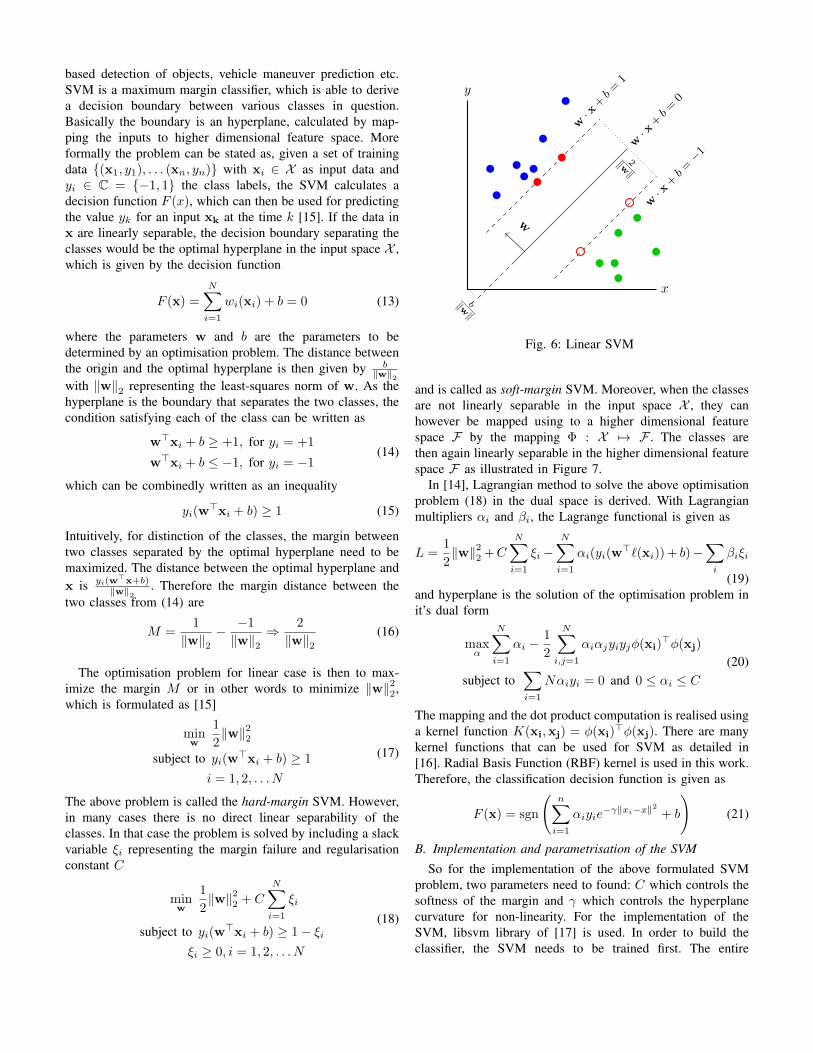
where the parameters w and b are the parameters to bedetermined by an optimisation problem. The distance betweenthe origin and the optimal hyperplane is then given by b

‖w‖2with ‖w‖2 representing the least-squares norm of w. As thehyperplane is the boundary that separates the two classes, thecondition satisfying each of the class can be written as

w>xi + b ≥ +1, for yi = +1

w>xi + b ≤ −1, for yi = −1(14)

which can be combinedly written as an inequality

yi(w>xi + b) ≥ 1 (15)

Intuitively, for distinction of the classes, the margin betweentwo classes separated by the optimal hyperplane need to bemaximized. The distance between the optimal hyperplane andx is yi(w

>x+b)‖w‖2

. Therefore the margin distance between thetwo classes from (14) are

M =1

‖w‖2− −1

‖w‖2⇒ 2

‖w‖2(16)

The optimisation problem for linear case is then to max-imize the margin M or in other words to minimize ‖w‖22,which is formulated as [15]

minw

1

2‖w‖22

subject to yi(w>xi + b) ≥ 1

i = 1, 2, . . . N

(17)

The above problem is called the hard-margin SVM. However,in many cases there is no direct linear separability of theclasses. In that case the problem is solved by including a slackvariable ξi representing the margin failure and regularisationconstant C

minw

1

2‖w‖22 + C

N∑i=1

ξi

subject to yi(w>xi + b) ≥ 1− ξi

ξi ≥ 0, i = 1, 2, . . . N

(18)

y

x

w· x+b=0

w· x+b=1

w· x+b=−12‖w‖

b‖w‖

w

Fig. 6: Linear SVM

and is called as soft-margin SVM. Moreover, when the classesare not linearly separable in the input space X , they canhowever be mapped using to a higher dimensional featurespace F by the mapping Φ : X 7→ F . The classes arethen again linearly separable in the higher dimensional featurespace F as illustrated in Figure 7.

In [14], Lagrangian method to solve the above optimisationproblem (18) in the dual space is derived. With Lagrangianmultipliers αi and βi, the Lagrange functional is given as

L =1

2‖w‖22 +C

N∑i=1

ξi−N∑i=1

αi(yi(w>`(xi)) + b)−

∑i

βiξi

(19)and hyperplane is the solution of the optimisation problem init’s dual form

maxα

N∑i=1

αi −1

2

N∑i,j=1

αiαjyiyjφ(xi)>φ(xj)

subject to∑i=1

Nαiyi = 0 and 0 ≤ αi ≤ C(20)

The mapping and the dot product computation is realised usinga kernel function K(xi,xj) = φ(xi)

>φ(xj). There are manykernel functions that can be used for SVM as detailed in[16]. Radial Basis Function (RBF) kernel is used in this work.Therefore, the classification decision function is given as

F (x) = sgn

(n∑i=1

αiyie−γ‖xi−x‖2 + b

)(21)

B. Implementation and parametrisation of the SVM

So for the implementation of the above formulated SVMproblem, two parameters need to found: C which controls thesoftness of the margin and γ which controls the hyperplanecurvature for non-linearity. For the implementation of theSVM, libsvm library of [17] is used. In order to build theclassifier, the SVM needs to be trained first. The entire

y

x

Φ : X 7→ F

x

y

z

Fig. 7: Non-linear SVM

feature data with 2658 samples is scaled to the range [0, 1]as recommended by the authors of libsvm. 66.6% of the dataset is divided as training data and the remaining 33.3% astesting data. The multi-class classification problem is solved asone-vs-rest classification problem in libsvm. Before the actualtraining of classifier, the parameters need to be estimated bycross-validation method. Cross-validation is the method ofdividing the training set into certain fold of subsets, trainthe classifier with a set of subsets and sequentially test theclassifier with one subset which was not used in training.

Grid-search on C and γ using cross-validation is recom-mended in [17] and used so in this work. Sequences of (C, γ)are tried and the one with the best cross-validation accuracyis selected. Initially a rough grid-search with 3-fold cross-validation and step-size 2 is made with broad (C, γ) rangesC = 2−20, 2−18, . . . , 220 and γ = 2−20, 2−18, . . . , 220. Thisis to roughly find the parameter regions where the cross-validation accuracy is high. As depicted in Figure 8, the bestpair obtained is (218, 22) with cross-validation accuracy of84.3115% and the regions bounded by C = 2−4, . . . , 220

and γ = 2−12, . . . , 212 has higher cross-validation accuracy.However, the number of support vectors (SV) increases by

-20 -18 -16 -14 -12 -10 -8 -6 -4 -2 0 2 4 6 8 10 12 14 16 18 20

-20

-18

-16

-14

-12

-10

-8

-6

-4

-2

0

2

4

6

8

10

12

14

16

18

20

Log2γ

Log

2c

50 60 70 80

CV Accuracy %

Fig. 8: Rough RBF-Kernel parameter search by cross-validation with step-size 2

increasing the slack value i.e. C. This consequently increasesthe prediction complexity because for every test point, a dotproduct with each SV needs to be computed. On the otherhand, a very low value of C would increase misclassification.A higher value for γ would result in over-fitting and a verylow value would not reflect the non-linearity in the decisionboundary. Therefore a trade-off is to be made between thecross-validation accuracy and kernel parameters. So in thesecond medium-scale grid-search the scale of (C, γ) is reducedto the range C = 2−2, 2−1, . . . , 218 and γ = 2−6, 2−5, . . . , 28

with a step-size 1. The best pair from medium scale searchis (216, 23), with cross-validation accuracy of 84.0293%, asshown in Figure 9. Finally, the search is narrowed down tothe region C = 24, 23.75, . . . , 213 and γ = 2−2, 2−1.75, . . . , 26

with a step-size 0.25, as depicted in Figure 10 and the bestparameter is found to be (213, 23.5) with a cross-validationaccuracy of 82.9007%. Considering the trade-off, the parame-ter pair (210.5, 24.25) providing a cross-validation accuracy of81% is chosen for training the model, along the direction ofbest parameter in the grid.

V. EXPERIMENTS AND RESULTS

A. Properties

A data set consisting of detections from a prototype radarsensor with a carrier frequency of the range 77-81 GHz isused. The range and Doppler of a target are measured byFMCW principle. The used radar has an opening angle of±75°, angular resolution of 1°and range resolution of 0.1m.The radar sensor delivers measurements in polar coordinateswith azimuth, range and relative velocity values of objects.The FoV covered by the radar sensor as mounted on the right

-6 -5 -4 -3 -2 -1 0 1 2 3 4 5 6 7 8

-2

-1

0

1

2

3

4

5

6

7

8

9

10

11

12

13

14

15

16

Log2γ

Log

2c

50 60 70 80

CV Accuracy %

Fig. 9: Medium scale RBF-Kernel parameter search by cross-validation with step-size 1

-2 -1.5 -1 -0.5 0 0.5 1 1.5 2 2.5 3 3.5 4 4.5 5 5.5 6

4

5

6

7

8

9

10

11

12

13

Log2γ

Log

2c

70 75 80

CV Accuracy %

Fig. 10: Small scale RBF-Kernel parameter search by cross-validation with step-size 0.25.

corner of the vehicle is illustrated in Figure 11. Further, theobject classes of interest are pedestrian, bicyclist and passengercar. Many sets of measurement are made for each object class,with different maneuvers, in order to capture a wide spread offeature data. A bigger test area of radius more than 60 mis chosen in order to avoid the reflections that could comefrom other objects in the test area, which would cause abias in feature extraction. However, sensor clutter cannot beavoided explicitly but are removed from measurements similarto the preprocessing method explained in section II. After these

Fig. 11: Radar sensor field of view

pre-processing steps, a total of 2658 labelled cluster samplesare considered further for feature extraction and also for theclassifier training.

B. Clustering results

Considering the properties of the used radar sensor, theparameters Eps and MinPts required for DBSCAN algorithmare chosen as 3 and 0.05 m respectively. A snapshot of thescenario for testing detections clustering and the correspondingresult is shown in Figure 12. In the shown test scenario, abicyclist moves parallel to the ego-vehicle. The sequence isrecorded in a yard, where a large wall and metal doors in thebackground, which are also detected and grouped as distinctclusters. Although the radar delivers only lesser detection

−20 −10 0 10−30

−20

−10

0

x [m]

y[m

]

Fig. 12: Snapshot of a test sequence showing the results ofdetections clustering with DBSCAN. In the top Figure thecluster detections belonging to bicyclist are indicated by redmarkers, cluster detections belonging to corner of building areindicated in blue markers and unclustered individual detectionsin yellow. Bottom Figure is the corresponding web-cam snap-shot

points compared to other high resolution sensors like laser

Fig. 13: Example measurement scenario illustrating geometricshape fit.

scanner, the results show that the clustering is still feasiblewith effective heuristics. Distinction of objects when they aretoo close to each other is possible only to a certain extentusing a single radar sensor. Also, when a poor reflectingclass like pedestrian is very close to other object class withhigh reflectivity like a passenger car, it may happen that theinterference is high and the pedestrian may not be detected atall. In addition to the radar sensor, using multiple sensors likecamera or laser scanner and fusion of detections from thesemultiple sensors would improve the object distinction.

C. Feature extraction results

Another test for evaluating the geometric shape and featureextraction was performed, this time also involving the pedes-trian and passenger car apart from the bicyclist. The shapefitting result is presented in Figure 13. The green boundingboxes belong to the passenger car, blue to the bicyclist andmagenta to the pedestrian. For clarity purpose, the shape fitof pedestrian and bicyclist are shown only for their forwardmotion.

D. Classification results

The confusion matrix of the SVM classifier for the pedes-trian, bicyclist and car classes are depicted in Figure 14. Therows of the confusion matrix represent the true class of theobject and the columns represent the predicted class. Thediagonal elements of the confusion matrix represent the true-positives (TP) of that specific class and the correspondingrow elements represent the false-negatives (FN). The car classhas the highest probability of TPs, where it is classifiedcorrectly for 88.2% of the time. The confusion of the carclass with pedestrian class is 0 %, whereas there is a smallconfusion of 11.8 % with the bicyclist class because thebicyclist samples include Doppler measurements overlappingwith the car class. The pedestrian class is classified correctly76.23 % of the time and the bicyclist is classified correctly71.25 % of the time. There is relatively larger confusionbetween the pedestrian and the bicyclist class because manyof the features from radar detections are identical to both ofthe classes, although the Doppler difference is wider. As both

Fig. 14: Confusion Matrix representing the results of radarbased object classification. Numbers represent the probabilityvalues.

pedestrians and bicyclists are relevant objects for most of theaccident avoidance applications like an urban turning assist,it is important to reduce the false alarms due to irrelevantobjects like a passenger car. This requirement can very wellbe satisfied by the developed classifier.

VI. CONCLUSION

This paper presented an approach to classify road usersbased on high-resolution radar sensors for autonomous driv-ing applications. The suggested procedure begins with pre-processing the radar detections and outputs the class ofthe objects in the vehicle environment. After an initial pre-processing, the radar detections were clustered into distinctgroups using DBSCAN clustering algorithm. Apart fromthe geometric features, different radar specific characteristicfeatures were defined and consequently extracted for eachof the detection clusters. A SVM classifier was constructedand parametrised, which takes the extracted features as aninput and gives the class probability of the object as output.The clustering, feature extraction and classification perfor-mance were demonstrated based on different evaluations. Theclassifier shows promising results for separating passengercars, bicyclists and pedestrians. However, there is still highconfusion between the pedestrian and bicyclist classes. Thiscan be improved in the future by using different classificationapproaches such as deep neural networks and also by using abigger dataset recorded with mutiple radar sensors.

REFERENCES

[1] D. Stuker, Heterogene Sensordatenfusion zur robusten Objektverfolgungim automobilen Straßenverkehr. PhD dissertation, Carl von Ossietzky-UniversityOldenburg, 2006.

[2] M. Munz, Generisches Sensorfusionsframework zur gleichzeitigenZustands-und Existenzschatzung fur die Fahrzeugumfelderkennung. PhDdissertation,Ulm University, 2011.

[3] E. Schubert, M. Kunert, A. Frischen and W.A. Menzel, Multi-Reflection-Point Target Model for Classification of Pedestrians by AutomotiveRadar. In:Proceedings of the 11th European Radar Conference, pages181–184, 2014.

[4] F. Folster, Erfassung ausgedehnter Objekte durch ein Automobil-Radar.PhD Dissertation, Technical University Hamburg-Harburg, 2006.

[5] N. Kampchen, Feature-level fusion of laser scanner and video data foradvanced driver assistance systems. PhD dissertation, Ulm University,2007.

[6] H. Zhao, X.W. Shao, K. Katabira and R. Shibasaki, Joint tracking and-classification of moving objects at intersection using a single-row laserrange scanner, in:Proceedings of the IEEE Intelligent TransportationSystems Con-ference, pages 287–294, 2006.

[7] C. Premebida, O. Ludwig, and U. Nunes, Exploiting LIDAR-basedFeatures on Pedestrian Detection in Urban Scenarios. In:Proceedings ofthe 12th Inter-national IEEE Conference on Intelligent TransportationSystems, pages 18–23, 2009.

[8] M. Ester, H.P. Kriegel, J. Sander and X. Xu, A Density-Based Algo-rithm for Discovering Clusters in Large Spatial Databases with Noise.in:Proceedingsof KDD, vol. 96, pages 226–231, 1996.

[9] V. Nguyen, A. Martinelli, N. Tomatis and R. Siegwart. A comparison ofline extraction algorithms using 2D laser rangefinder for indoor mobilerobotics. In: IEEE/RSJ Conference on Intelligent Robotics and Systems,2005.

[10] K. O. Arras, O. M. Mozos and W. Burgard. Using Boosted Featuresfor the Detection of People in 2D Range Data. In: IEEE InternationalConference on Robotics and Automation, pages 3402–3407, 2007.

[11] C. Premebida, O. Ludwig and U. Nunes. Exploiting LIDAR-basedFeatureson Pedestrian Detection in Urban Scenarios. In:Proceedings ofthe 12th Inter-national IEEE Conference on Intelligent TransportationSystems, pages 18–23,2009.

[12] S. Pietzsch. Modellgestutzte Sensordatenfusion von Laserscanner undRadar zur Erfassung komplexer Fahrzeugumgebungen. PhD dissertation,TechnicalUniveristy Munich, 2015.

[13] C. Li, J. Wang, L. Wang, L. Hu and P. Gong. Comparison of Classifica-tion Algorithms and Training Sample Sizes in Urban Land Classificationwith Landsat Thematic Mapper Imagery. In: Remote Sensing, vol. 6, no.2, pages 964–983, 2014.

[14] C. Cortes and V. Vapnik. Support-Vector Networks. In: Machine Learn-ing, pages 273–297, 1995.

[15] B. E. Boser, I. M. Guyon, V. N. and Vapnik. A Training Algorithm forOptimal Margin Classifiers. In: Proceedings of the Fifth Annual Work-shop on Computational Learning Theory, COLT ’92, pages 144–152,New York, NY, USA, 1992. ACM.

[16] M. Hoffmann, Support Vector Machines — Kernels and the KernelTrick, 2006.

[17] C.-C. Chang and C.-J. Lin, LIBSVM: a Library for SupportVector Machines, Initial version: 2001 & Updated version 2013.https://www.csie.ntu.edu.tw/ cjlin/libsvm/.

high-resolution radar based object classiﬁcation for

Documents