This content has been downloaded from IOPscience. Please scroll down to see the full text.

Download details:

IP Address: 155.97.178.73

This content was downloaded on 24/06/2014 at 10:57

Please note that terms and conditions apply.

High-resolution distributed-feedback fiber laser dc magnetometer based on the Lorentzian

force

View the table of contents for this issue, or go to the journal homepage for more

2009 Meas. Sci. Technol. 20 034023

(http://iopscience.iop.org/0957-0233/20/3/034023)

Home Search Collections Journals About Contact us My IOPscience

IOP PUBLISHING MEASUREMENT SCIENCE AND TECHNOLOGY

Meas. Sci. Technol. 20 (2009) 034023 (11pp) doi:10.1088/0957-0233/20/3/034023

High-resolution distributed-feedbackfiber laser dc magnetometer based on theLorentzian force

G A Cranch1, G M H Flockhart1 and C K Kirkendall

Naval Research Laboratory, 4555 Overlook Avenue SW, Washington, DC 20375, USA

E-mail: geoff.cranch@nrl.navy.mil

Received 6 June 2008, in final form 14 July 2008Published 4 February 2009Online at stacks.iop.org/MST/20/034023

Abstract

A low-frequency magnetic field sensor, based on a current-carrying beam driven by theLorentzian force, is described. The amplitude of the oscillation is measured by adistributed-feedback fiber laser strain sensor attached to the beam. The transductionmechanism of the sensor is derived analytically using conventional beam theory, which isshown to accurately predict the responsivity of a prototype sensor. Excellent linearity andnegligible hysteresis are demonstrated. Noise sources in the fiber laser strain sensor aredescribed and thermo-mechanical noise in the transducer is estimated. The prototype sensorachieves a magnetic field resolution of 5 nT Hz for 25 mA of current, which is shown to beclose to the predicted thermo-mechanical noise limit of the sensor. The current is suppliedoptically through a separate optical fiber yielding an electrically passive sensor head.

Keywords: DFB fiber laser, fiber-optic sensor, magnetometer, thermal noise, Lorentz force

(Some figures in this article are in colour only in the electronic version)

1. Introduction

Fiber-optic interferometric sensors have become anestablished technology for Naval underwater acousticapplications. Both platform-mounted systems [1] and seabed-mounted systems [2, 3] have been developed. Fiber-opticsensor-based seabed-mounted hydrophone arrays offer thepotential for very large area coverage with a lightweight,rapidly deployable system. The optical fiber link is capableof carrying information from a large number of fiber-opticsensors (several hundred) to a remotely located shore stationor surface mooring. Passive target detection by acousticsignature measurement forms the basis of many sonar systems.However, detection of targets by other associated signaturessuch as electric or magnetic field is also possible [4]. Thiscan be particularly advantageous in areas of high acousticreverberation and noise where acoustic detection ranges arelimited. An underwater array consisting of a combination ofsensors may therefore, in certain circumstances, provide animproved detection capability.

1 Employed by SFA Inc., Crofton, MD 21114, USA.

Fiber-optic-sensor-based magnetometers have manyfavorable attributes for applications requiring multi-point,remote measurements of low-frequency magnetic fields. Anundersea magnetometer requiring no electrical power is highlydesirable to improve reliability and to enable remote locationof the sensors. The sensors are connected by a fiber-optic link free from electromagnetic interference and do notradiate any electric or magnetic fields of their own. Afiber-optic magnetometer has previously been demonstratedthat uses a magnetostrictive material to convert the magneticfield into a strain, which is measured interferometrically [5].The magnetostrictive material was a transversely annealedMetglass cylinder around which an optical fiber is wound.This is placed in one arm of an interferometer whichmeasures the strain generated in the presence of a magneticfield. The response of the Metglass to the magnetic fieldis quadratic, such that by applying an ac magnetic ditherfield to the transducer (typically up to 20 kHz) the low-frequency magnetic field of interest appears as modulationsidebands on a carrier at the dither frequency. Low-frequencymagnetic field resolutions of 3 pT Hz−1/2 at 10 Hz [6]

0957-0233/09/034023+11$30.00 1 © 2009 IOP Publishing Ltd Printed in the UK

Meas. Sci. Technol. 20 (2009) 034023 G A Cranch et al

and 38 pT Hz−1/2 at 0.1 Hz [7] have been demonstrated,which compares very well to high performance flux-gatemagnetometers achieving low-frequency resolutions around1–10 pT Hz−1/2 [8]. However, magnetostrictive Metglassprovides a far from ideal strain response. It has beenobserved that these materials can exhibit both a significantresidual signal in the absence of a magnetic field, whichcan be equivalent to several microtesla, and 1/f sidebandnoise associated with dynamic processes in the Metglass [9].Although methods based on the choice of dither frequencyand annealing conditions have been found to reduce theseeffects, it is generally necessary to operate the sensor closedloop, maintaining the magnetostrictive at its zero internalfield point, to overcome hysteresis and the residual signalin the magnetostrictive [10]. The fiber-optic interferometermust also be –quadrature locked in order to achieve sub-microradian phase resolution. For a three-axis magnetometer,a total of four feedback loops are required resulting in arelatively complex sensor head when the associated electronicsfor the feedback loops are included. An array of eight three-axis magnetometers demonstrated magnetic field resolutionsof 0.2 nT Hz−1/2 at 0.1 Hz limited by residual 1/f noise[5]. Although laboratory-based sensors have demonstratedsignificantly improved performance, consistent improvementin sensitivity has not yet been achieved. The need to provideelectrical power and feedback signals to the sensor head is asignificant disadvantage, particularly when the sensors are tobe located several kilometers from the interrogation system.

An alternative transduction mechanism for a fiber-opticmagnetometer has also been demonstrated previously, basedon the Lorentzian force generated in a current-carryingconductor in the presence of a magnetic field [11]. A variantof this sensing concept has recently been demonstrated bythe authors [12, 13], which uses a distributed-feedback (DFB)fiber laser strain sensor to measure the strain induced in avibrating metal beam carrying an ac dither current in thepresence of a quasi-dc magnetic field. The DFB fiber laserstrain sensor provides an order of magnitude increase in strainresolution compared with the remotely interrogated fiber-opticinterferometer, for very short lengths of fiber [14]. This makesit ideally suited for this transduction mechanism, where theinteraction length is typically a few centimeters. Bending ofthe beam induces a flexural strain in the fiber in proportionto the Lorentzian force acting on the beam. This force isproportional to the product of the magnetic field strengthand current, yielding an ac strain proportional in amplitudeto the magnetic field. This transduction mechanism shouldyield no residual signal for zero applied field and is shown toexhibit no measurable hysteresis. Thus, it should be possibleto achieve a stable, drift-free magnetic field measurementwith a sensor operating open loop. An added benefit isthat the responsivity of the sensor is proportional to thecurrent; thus an increase in current will yield a proportionalincrease in responsivity and sensitivity. The strain inducedin the fiber laser modulates the laser emission frequency,which can be converted into an intensity modulation withan imbalanced fiber-optic interferometer located with theinterrogation electronics. Thus, no feedback signal is required

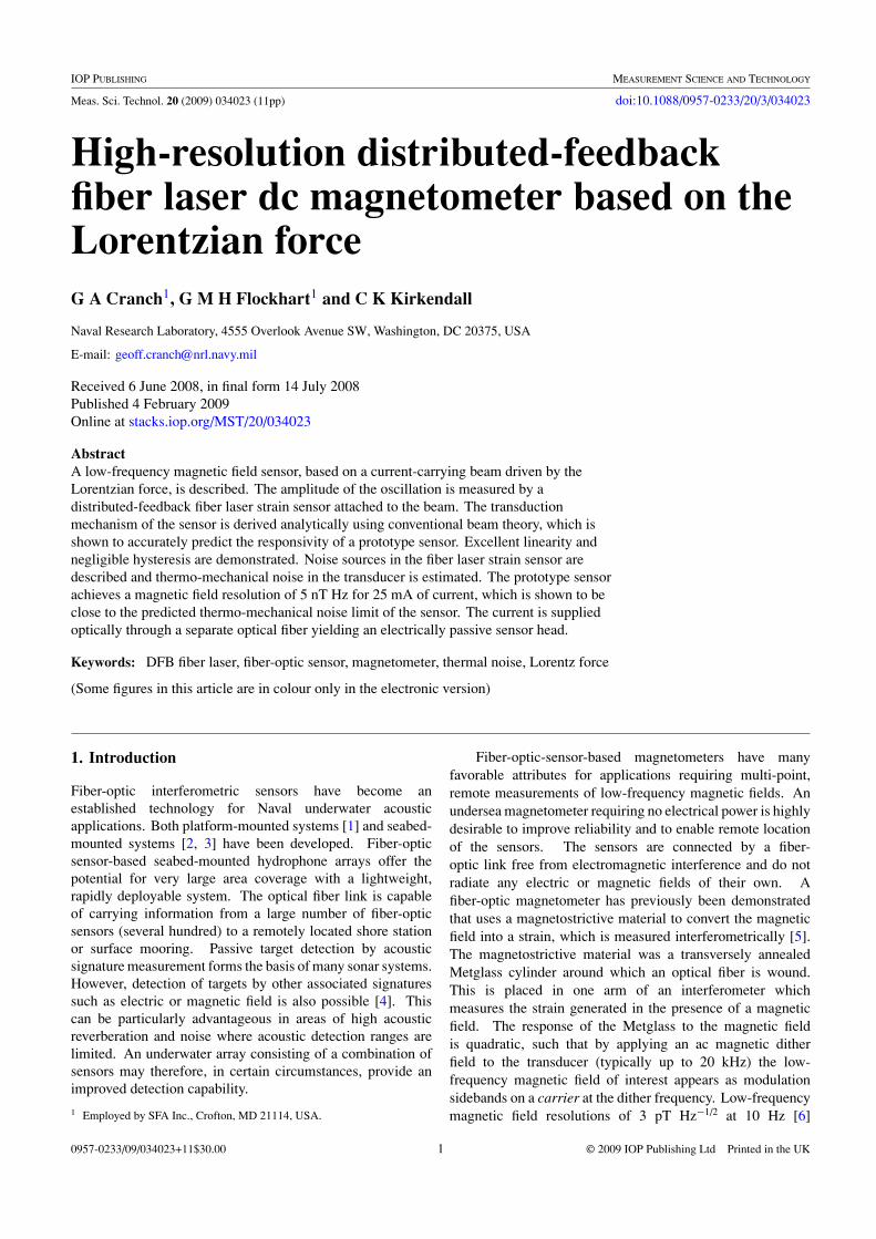
Figure 1. DFB fiber laser configuration (top) longitudinal spatialmode profile of the fiber laser.

at the sensor head. The required dither current can be suppliedoptically removing the need to transmit electrical power to thesensor head.

This paper describes in detail the fiber laser magnetometer.It is arranged as follows. Section 2 describes the operatingprinciple of the distributed-feedback fiber laser sensor.Section 3 describes the mechanical transducer, identifies thetransduction mechanism and derives the sensor responsivityusing conventional beam theory applied to a compositestructure. Section 4 describes a prototype sensor and themethod used to demodulate the strain signal from the fiberlaser sensor. Section 5 estimates the thermo-mechanicallyinduced displacement noise in the transducer and presents themeasured noise properties of the sensor. Finally, conclusionsare summarized in section 6.

2. DFB fiber laser sensing principle

The DFB fiber laser configuration is shown in figure 1. Itconsists of a length of single-mode, photosensitive erbium-doped fiber (EDF) within which a Bragg grating is formed. Thedistributed-feedback structure is a λ/4 configuration, formedwith a single π phase shift in the center of the grating. Thegrating is formed by scanning a UV beam (244 nm) acrossa phase mask. Each end of the doped fiber is spliced toa passive fiber (e.g., SMF-28TM) and the erbium is pumpedwith a semiconductor laser at 980 nm. The laser emissionwavelength is determined primarily by the pitch of the grating,�, according to the Bragg condition, λB = 2n�, where nis the effective index of the optical fiber and can be set towithin the Er3+ window (1525–1560 nm). Slope efficienciesmeasured as the ratio of emission power to input pump powerare typically less than 1% dependent on the gain characteristicsof the erbium fiber and the grating properties [16]. The laserstructure supports a single fundamental mode, the center ofwhich is located about the phase shift and thus emits a singlefrequency. The spatial mode intensity profile, I(x), is shownin the upper plot of figure 1. For the ideal case of a uniformgrating with a π phase shift in the center, the mode intensityis described by I (x) = Io exp(−2κ|x|), where x is the axialcoordinate along the fiber. The effective cavity length can beshown to be given by Lc = 1/κ [15], where κ is the amplitudeof the coupling coefficient of the grating.

2

Meas. Sci. Technol. 20 (2009) 034023 G A Cranch et al

yConductingstrip

DFB fiber laser

Fixed Support

B

( ) ( )BF t B i t

BFgF

zx

i(t) Adjustable

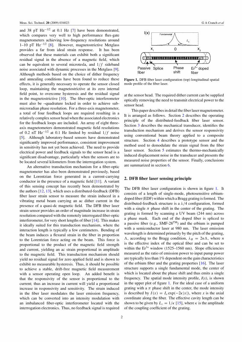
Figure 2. Lorentzian-force-based magnetic field sensorconfiguration.

If a localized strain profile, described by �ε(x, t), isapplied to the fiber, the normalized frequency shift is givenby [15]

�νs

νs

= (0.78) κ

∫ x2

x1

�ε(x, t) exp(−2κ |x|) dx. (1)

The measurement resolution of the DFB fiber laser sensor islimited by the frequency noise of the emitted radiation. Thetypical frequency noise spectra for this laser can be found in[16]. The spectral density of the frequency noise exhibits a1/f n (n ≈ 0.5) spectrum at frequencies below 1 kHz and istypically 40 Hz Hz−1/2 at 100 Hz and 20 Hz Hz−1/2 at 1 kHz.

3. Lorentzian-force-based sensor model

The sensor comprises a DFB fiber laser attached to aconducting metal strip, as illustrated in figure 2. The DFBfiber laser is 50 mm in length with a centrally located π phaseshift. The phase shift is positioned to be in the center of thebeam, and the beam and fiber are clamped at each end. Thecoupling coefficient, κ , for the laser used in the experimentsis ∼200 m−1.

The responsivity of the sensor can be derived byconsidering the static and dynamic deflections of the beamunder a uniform load.

3.1. Static and dynamic deflection properties of the beam

The deflection, y, of an elastic beam is related to the momentsacting on the beam M(x) through the flexure equation [17],

M(x) = EIz

d2x

dy2, (2)

where E is Young’s modulus and Iz is the second moment ofthe area of the beam. For a beam of length l, fixed at each endsubjected to a uniform load per unit length, F, under zero axialtension, the moments are given by

M(x) = F l

2x +

F l2

12− Fx

(x

2

), (3)

where the first term is a torque due to the reaction force, RA,at the edge of the beam, the second term is a torque, MA, dueto the end constraint and the third term is a torque due to theuniform applied load, F. The x coordinate extends from zeroto l. Substituting (3) into (2), integrating once and using the

Figure 3. Beam configuration.

condition (dy/dx)|x=0 = 0 for a fixed end boundary conditionyields the beam tangent:

θ(x) = F

EI

(−1

6x3 +

l

4x2 − l2

12x

). (4)

The beam shape, y(x), can be obtained from a furtherintegration of the beam tangent and applying the boundarycondition y(x)|x=0 = 0, yielding

y(x) = F

EI

(− 1

24x4 +

l

12x3 − l2

24x2

). (5)

Assuming that the beam is orientated with its flat face normalto the gravitational force, the applied load per unit length,F, comprises two components, Fg + �FB . Fg is the forcedue to gravity and �FB is the Lorentzian force, which for acurrent carrying conductor is equal to B · i, where B is themagnetic field induction (flux density) and is equal to μ0H,

where H is the magnetic field strength and μ0 is the magneticpermeability. i is the current in the conducting strip.

The dynamic deflection of the beam can be calculatedfrom the Euler equation for beams, by assuming simpleharmonic motion for the driving force such that F = ηω2y,where η is the mass per unit length and ω is the excitationfrequency. This yields [18]

d4y

dx4− β4y = F. (6)

Here the term β = ηω2/EI has been introduced. The naturalfrequencies of vibration ωn can be obtained from

ωn = (βnEIz/η)1/2, (7)

where the constant β1 determined from the boundaryconditions is β1 = (16/3)π4 for the first resonance of a beamfixed at each end [18].

3.2. Calculating EI for the composite beam structure

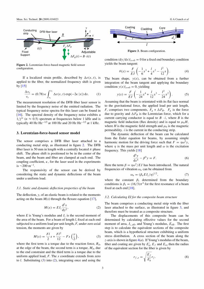
The beam comprises a conducting metal strip with the fiberlaser attached to the surface, as illustrated in figure 3, andtherefore must be treated as a composite structure.

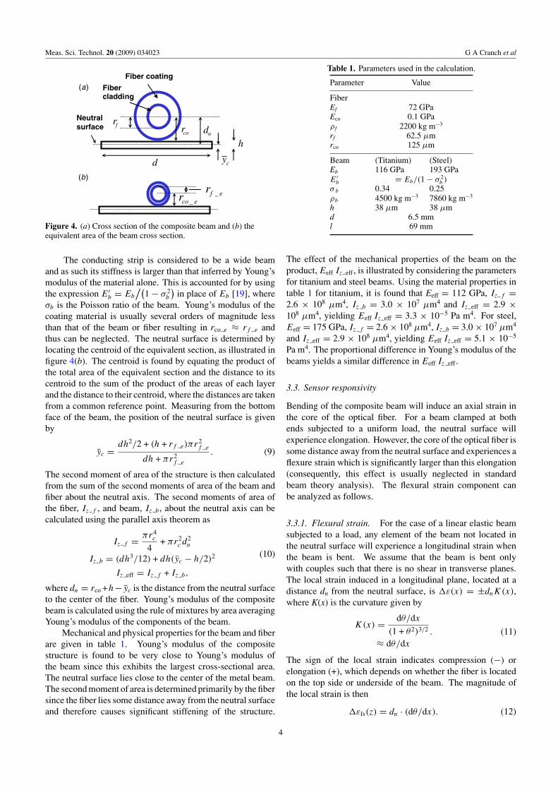
The displacements of this composite beam can bedetermined by calculating effective values for the secondmoment of area, Iz eff , and Young’s modulus, Eeff . The firststep is to calculate the equivalent sections of the compositebeam, which is a hypothetical structure exhibiting a uniformstress distribution. A cross section of the beam along thez-axis is shown in figure 4(a). If Young’s modulus of the beam,fiber and coating are given by E′

b, Ef and Eco then the radiusof the equivalent section for the fiber is given by

rf e =√

Ef

E′b

rf . (8)

3

Meas. Sci. Technol. 20 (2009) 034023 G A Cranch et al

Neutral surface

nd

Fiber coating

Fibercladding

corfr

_co er _f er

(a)

(b)

h

d cy

Figure 4. (a) Cross section of the composite beam and (b) theequivalent area of the beam cross section.

The conducting strip is considered to be a wide beamand as such its stiffness is larger than that inferred by Young’smodulus of the material alone. This is accounted for by usingthe expression E′

b = Eb

/(1 − σ 2

b

)in place of Eb [19], where

σb is the Poisson ratio of the beam. Young’s modulus of thecoating material is usually several orders of magnitude lessthan that of the beam or fiber resulting in rco e ≈ rf e andthus can be neglected. The neutral surface is determined bylocating the centroid of the equivalent section, as illustrated infigure 4(b). The centroid is found by equating the product ofthe total area of the equivalent section and the distance to itscentroid to the sum of the product of the areas of each layerand the distance to their centroid, where the distances are takenfrom a common reference point. Measuring from the bottomface of the beam, the position of the neutral surface is givenby

yc = dh2/2 + (h + rf e)πr2f e

dh + πr2f e

. (9)

The second moment of area of the structure is then calculatedfrom the sum of the second moments of area of the beam andfiber about the neutral axis. The second moments of area ofthe fiber, Iz f , and beam, Iz b, about the neutral axis can becalculated using the parallel axis theorem as

Iz f = πr4c

4+ πr2

c d2n

Iz b = (dh3/12) + dh(yc − h/2)2

Iz eff = Iz f + Iz b,

(10)

where dn = rco +h− yc is the distance from the neutral surfaceto the center of the fiber. Young’s modulus of the compositebeam is calculated using the rule of mixtures by area averagingYoung’s modulus of the components of the beam.

Mechanical and physical properties for the beam and fiberare given in table 1. Young’s modulus of the compositestructure is found to be very close to Young’s modulus ofthe beam since this exhibits the largest cross-sectional area.The neutral surface lies close to the center of the metal beam.The second moment of area is determined primarily by the fibersince the fiber lies some distance away from the neutral surfaceand therefore causes significant stiffening of the structure.

Table 1. Parameters used in the calculation.

Parameter Value

FiberEf 72 GPaEco 0.1 GPaρ f 2200 kg m−3

rf 62.5 μmrco 125 μm

Beam (Titanium) (Steel)Eb 116 GPa 193 GPaE′

b = Eb/(1 − σ 2b )

σ b 0.34 0.25ρb 4500 kg m−3 7860 kg m−3

h 38 μm 38 μmd 6.5 mml 69 mm

The effect of the mechanical properties of the beam on theproduct, Eeff Iz eff , is illustrated by considering the parametersfor titanium and steel beams. Using the material properties intable 1 for titanium, it is found that Eeff = 112 GPa, Iz f =2.6 × 108 μm4, Iz b = 3.0 × 107 μm4 and Iz eff = 2.9 ×108 μm4, yielding Eeff Iz eff = 3.3 × 10−5 Pa m4. For steel,Eeff = 175 GPa, Iz f = 2.6 × 108 μm4, Iz b = 3.0 × 107 μm4

and Iz eff = 2.9 × 108 μm4, yielding Eeff Iz eff = 5.1 × 10−5

Pa m4. The proportional difference in Young’s modulus of thebeams yields a similar difference in Eeff Iz eff .

3.3. Sensor responsivity

Bending of the composite beam will induce an axial strain inthe core of the optical fiber. For a beam clamped at bothends subjected to a uniform load, the neutral surface willexperience elongation. However, the core of the optical fiber issome distance away from the neutral surface and experiences aflexure strain which is significantly larger than this elongation(consequently, this effect is usually neglected in standardbeam theory analysis). The flexural strain component canbe analyzed as follows.

3.3.1. Flexural strain. For the case of a linear elastic beamsubjected to a load, any element of the beam not located inthe neutral surface will experience a longitudinal strain whenthe beam is bent. We assume that the beam is bent onlywith couples such that there is no shear in transverse planes.The local strain induced in a longitudinal plane, located at adistance dn from the neutral surface, is �ε(x) = ±dnK(x),where K(x) is the curvature given by

K(x) = dθ/dx

(1 + θ2)3/2

≈ dθ/dx

. (11)

The sign of the local strain indicates compression (−) orelongation (+), which depends on whether the fiber is locatedon the top side or underside of the beam. The magnitude ofthe local strain is then

�εfs(z) = dn · (dθ/dx). (12)

4

Meas. Sci. Technol. 20 (2009) 034023 G A Cranch et al

0 10 20 30 40 50 60 70

0.00

0.05

0.10

0.15

0 10 20 30 40 50 60 70-10

-5

0

5

10

Lo

cal s

tra

in,

Δε(x

) [μ

m]

Re

spo

nsi

vity

, [H

z/n

T/m

A]

Phase shift position, [mm]

κ =100m-1

Figure 5. Local strain versus position for a beam under uniformload due to its weight and responsivity as a function of thephase-shift location for the Ti beam.

The responsivity of the sensor is derived by substituting (12)and (4) into (1) to yield

�νs

νs

= (0.78) κdn

F

EI

∫ l

0

(−1

2x2 +

l

2x − l2

12

)× exp(−2κ|x − xφ|) dx, (13)

where xφ is the position of the phase shift relative to the edgeof the beam. The length of the grating is set to be equal tothe supported length of the beam. The term in the integralevaluates to a constant dependent on the position and shape ofthe laser mode. If the beam is orientated such that its flat faceis normal to the gravitational force, then the total force per unitlength acting on the beam is the sum of the gravitation force,Fg , and the Lorentzian force, �FB . Injecting an ac currentyields a time-varying force such that �FB = Bi cos(ωdt).The beam will vibrate at the ac frequency, ωd , and the strainmeasured by the laser becomes a tone at this frequency, theamplitude of which is proportional to the magnetic field, B.The component of the laser frequency modulation at the ditherfrequency, referred to as the Lorentz tone, is

�νs |ωd

νs

= (0.78) κdn

�FB

EI

∫ l

0

(−1

2x2 +

l

2x − l2

12

)× exp(−2κ|x − xφ|) dx. (14)

ωd is set to coincide with the mechanical resonance, ωn,of the transducer, which provides a significant mechanicalamplification of the responsivity. This also upconverts themagnetic field signal to a frequency above 1/f noise whichlimits the low-frequency strain resolution of the fiber lasersensor. For a composite beam under the load of its ownweight, the induced local strain is shown in figure 5, usingthe parameters given in table 1 for a titanium beam. Thecurvature is maximum in the center of the beam and changessign of approximately one quarter of the beam length fromeither end. Figure 5 also shows the responsivity of the sensordue to the flexure strain as a function of the position of thelaser phase shift and hence the laser spatial mode center. Herethe relationship �FB = �B · i has been used to express theresponsivity in units of Hz nT−1 mA−1. The responsivity ismaximum when the laser mode is located centrally on the

beam and falls to a minimum at the point when the curvaturecrosses zero.

Equation (14) can be evaluated for the case of a centrallylocated phase shift (xφ = l/2), which yields

1

νs

�νs

�B= (0.78)

dni

24κ2EeffIz eff

×{exp(−κl)[2κ2l2 + 6κl + 6] + κ2l2 − 6}. (15)

This can be simplified further to

1

νs

�νs

�B= (0.78)

dni

24κ2EeffIz eff{κ2l2[2 exp(−κl) + 1] − 6},

(16)

which is accurate to within ∼4% for κl � 4. For the specialcase of an infinitely strong grating (i.e. taking κ → ∞), suchthat exp(−2κ|x − xφ|) = ∣∣0 x �=xφ

1 x=xφ, (16) reduces to

1

νs

�νs

�B= (0.78)

dnl2i

24EeffIz eff, (17)

which overestimates the responsivity by ∼30%. Thus, theresponsivity reduces to being proportional to the distance of thefiber from the neutral axis, the product EeffIz eff and the squareof the length l. However, dn is not an entirely free parameter,since it is related to the product EeffIz eff . In general, anincrease in responsivity can only be obtained by increasingthe device length, l, reducing the beam stiffness or increasingthe current i.

The response of the composite beam to acceleration, �a,can be determined by substituting the inertial force into (13),given by Fa = η�a. This is important when consideringits sensitivity to environmental vibration. The ratio of thebeam response to magnetic field and the response to appliedacceleration is then simply given by the ratio i/η, where η isthe mass/unit length.

3.4. Effect of grating distortion on laser behavior

Figure 5 shows the spatial dependence of the local straininduced in the fiber along the beam for a beam under the load ofits own weight. This strain variation has the undesirable effectof changing the local Bragg period along the grating and canstrongly affect the lasing behavior. Distortion of the gratingwill affect both the laser threshold and emission wavelength.To quantify this effect, the behavior of a DFB laser comprisinga uniform, π phase-shifted grating subjected to increasingbeam deflection is modeled using the F-matrix [20]. The FBGis described by the complex coupling coefficient, κ . The firststep is to calculate the phase of the coupling coefficient as afunction of the beam deflection. The local Bragg pitch of thegrating, ��(x), due to a local strain, �ε(x), is

��(x) = 0.78�B�ε(x), (18)

where �B is the grating pitch of the undistorted grating. Thephase of the coupling coefficient is then given by

arg(κ(x)) = 2π

�B

∫ x

0

(�B

�B + ��(x ′)− 1

)dx ′. (19)

The peak deflection of a beam under zero tension is given by�ymax = Fgl

4/(384EeffIz eff), where Fg is the weight per unit

5

Meas. Sci. Technol. 20 (2009) 034023 G A Cranch et al

0 10 20 30 40 50

0

1

2

3

Next higher order mode

Th

resh

old

fib

er

gain

[d

B/m

]

Peak deflection [micron]

Fundamental mode

Criticaldeflection

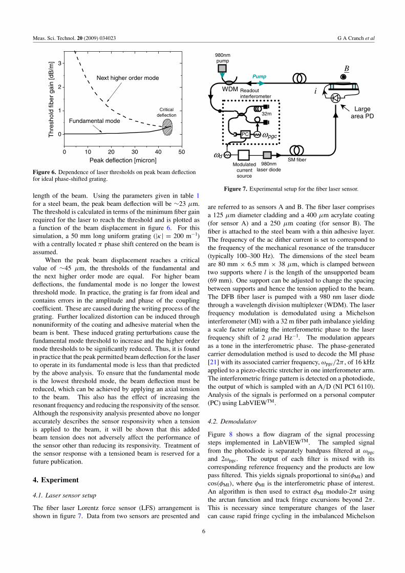
Figure 6. Dependence of laser thresholds on peak beam deflectionfor ideal phase-shifted grating.

length of the beam. Using the parameters given in table 1for a steel beam, the peak beam deflection will be ∼23 μm.The threshold is calculated in terms of the minimum fiber gainrequired for the laser to reach the threshold and is plotted asa function of the beam displacement in figure 6. For thissimulation, a 50 mm long uniform grating (|κ| = 200 m−1)with a centrally located π phase shift centered on the beam isassumed.

When the peak beam displacement reaches a criticalvalue of ∼45 μm, the thresholds of the fundamental andthe next higher order mode are equal. For higher beamdeflections, the fundamental mode is no longer the lowestthreshold mode. In practice, the grating is far from ideal andcontains errors in the amplitude and phase of the couplingcoefficient. These are caused during the writing process of thegrating. Further localized distortion can be induced throughnonuniformity of the coating and adhesive material when thebeam is bent. These induced grating perturbations cause thefundamental mode threshold to increase and the higher ordermode thresholds to be significantly reduced. Thus, it is foundin practice that the peak permitted beam deflection for the laserto operate in its fundamental mode is less than that predictedby the above analysis. To ensure that the fundamental modeis the lowest threshold mode, the beam deflection must bereduced, which can be achieved by applying an axial tensionto the beam. This also has the effect of increasing theresonant frequency and reducing the responsivity of the sensor.Although the responsivity analysis presented above no longeraccurately describes the sensor responsivity when a tensionis applied to the beam, it will be shown that this addedbeam tension does not adversely affect the performance ofthe sensor other than reducing its responsivity. Treatment ofthe sensor response with a tensioned beam is reserved for afuture publication.

4. Experiment

4.1. Laser sensor setup

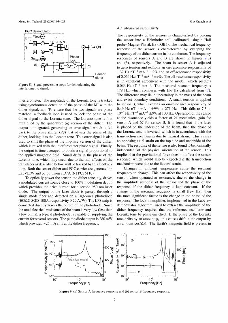
The fiber laser Lorentz force sensor (LFS) arrangement isshown in figure 7. Data from two sensors are presented and

Readout interferometer

Pump

B

i

Large area PD

WDM

SM fiber 980nm

laser diode

PC

32m

ωd

ωpgc

980nm pump

Modulated current source

Figure 7. Experimental setup for the fiber laser sensor.

are referred to as sensors A and B. The fiber laser comprisesa 125 μm diameter cladding and a 400 μm acrylate coating(for sensor A) and a 250 μm coating (for sensor B). Thefiber is attached to the steel beam with a thin adhesive layer.The frequency of the ac dither current is set to correspond tothe frequency of the mechanical resonance of the transducer(typically 100–300 Hz). The dimensions of the steel beamare 80 mm × 6.5 mm × 38 μm, which is clamped betweentwo supports where l is the length of the unsupported beam(69 mm). One support can be adjusted to change the spacingbetween supports and hence the tension applied to the beam.The DFB fiber laser is pumped with a 980 nm laser diodethrough a wavelength division multiplexer (WDM). The laserfrequency modulation is demodulated using a Michelsoninterferometer (MI) with a 32 m fiber path imbalance yieldinga scale factor relating the interferometric phase to the laserfrequency shift of 2 μrad Hz−1. The modulation appearsas a tone in the interferometric phase. The phase-generatedcarrier demodulation method is used to decode the MI phase[21] with its associated carrier frequency, ωpgc/2π , of 16 kHzapplied to a piezo-electric stretcher in one interferometer arm.The interferometric fringe pattern is detected on a photodiode,the output of which is sampled with an A/D (NI PCI 6110).Analysis of the signals is performed on a personal computer(PC) using LabVIEWTM.

4.2. Demodulator

Figure 8 shows a flow diagram of the signal processingsteps implemented in LabVIEWTM. The sampled signalfrom the photodiode is separately bandpass filtered at ωpgc

and 2ωpgc. The output of each filter is mixed with itscorresponding reference frequency and the products are lowpass filtered. This yields signals proportional to sin(φMI) andcos(φMI), where φMI is the interferometric phase of interest.An algorithm is then used to extract φMI modulo-2π usingthe arctan function and track fringe excursions beyond 2π .This is necessary since temperature changes of the lasercan cause rapid fringe cycling in the imbalanced Michelson

6

Meas. Sci. Technol. 20 (2009) 034023 G A Cranch et al

ωpgc

2ωpgc

ωd φ

1

t ∫

BPF LPF ATA N

PS

O/P

Sensor dither

φPS

∫q

i

PGC demodulator

Phase-lock

Figure 8. Signal processing steps for demodulating theinterferometric signal.

interferometer. The amplitude of the Lorentz tone is trackedusing synchronous detection of the phase of the MI with thedither signal, ωd . To ensure that the two signals are phasematched, a feedback loop is used to lock the phase of thedither signal to the Lorentz tone. The Lorentz tone is firstmultiplied by the quadrature (q) version of the dither. Theoutput is integrated, generating an error signal which is fedback to the phase shifter (PS) that adjusts the phase of thedither, locking it to the Lorentz tone. This error signal is alsoused to shift the phase of the in-phase version of the dither,which is mixed with the interferometer phase signal. Finally,the output is time averaged to obtain a signal proportional tothe applied magnetic field. Small drifts in the phase of theLorentz tone, which may occur due to thermal effects on thetransducer as described below, will be tracked by this feedbackloop. Both the sensor dither and PGC carrier are generated inLabVIEW and output from a D/A (NI PCI 6110).

To optically power the sensor, the dither tone, ωd , drivesa modulated current source close to 100% modulation depth,which provides the drive current for a second 980 nm laserdiode. The output of the laser diode is passed through asingle mode fiber and detected on a large-area photodiode(EG&G SGD-100A, responsivity 0.29 A/W). The LFS strip isconnected directly across the output of the photodiode. Sincethe total electrical resistance of the beam is very low (less thana few ohms), a typical photodiode is capable of supplying thecurrent for several sensors. The pump diode output is 280 mWwhich provides ∼25 mA rms at the dither frequency.

101

102

103

10-3

10-2

10-1

100

0

300

600

900

Ph

ase

[d

eg

]

Resp

on

sivi

ty [

Hz/

nT

/mA

]

Frequency [Hz]

Analytical model

101

102

103

10-4

10-3

10-2

10-1

100

0

300

600

900

Pha

se [d

eg

]

Re

spo

nsi

vity

[H

z/n

T/m

A]

Frequency [Hz]

Fit

(a) (b)

Figure 9. (a) Sensor A frequency response and (b) sensor B frequency response.

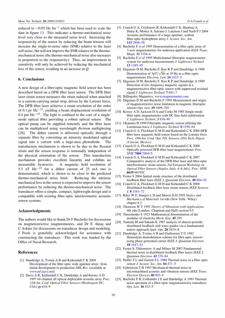
4.3. Measured responsivity

The responsivity of the sensors is characterized by placingthe sensor into a Helmholtz coil, calibrated using a Hallprobe (Magnet-Physik HS-TGB5). The mechanical frequencyresponse of the sensor is characterized by sweeping thefrequency of the dither current in the conductor. The frequencyresponses of sensors A and B are shown in figures 9(a)and (b), respectively. The beam in sensor A is adjustedto zero tension and exhibits an on-resonance responsivity of1.32 Hz nT−1 mA−1 ±9% and an off-resonance responsivityof 0.064 Hz nT−1 mA−1 ±9%. The off-resonance responsivityis in excellent agreement with the model, which predicts0.066 Hz nT−1 mA−1. The measured resonant frequency is178 Hz, which compares with 156 Hz calculated from (7).The difference may lie in uncertainty in the mass of the beamand exact boundary conditions. A small tension is appliedto sensor B, which exhibits an on-resonance responsivity of0.49 Hz nT−1 mA−1 ±9% at 271 Hz. This falls to 7.3 ×10−3 Hz nT−1 mA−1 ±9% at 100 Hz. Operation of the sensorat the resonance yields a factor of 21 mechanical gain forsensor A and 67 for sensor B. It is found that if the laseris placed on the underside of the beam, then the phase ofthe Lorentz tone is inverted, which is in accordance with thetransduction mechanism due to flexural strain. This causesan opposing axial strain on the top side and underside of thebeam. The response of the sensor is also found to be nominallyindependent of the physical orientation of the sensor. Thisimplies that the gravitational force does not affect the sensorresponse, which would also be expected if the transductionmechanism were due to the flexural strain.

Changes in ambient temperature cause the resonantfrequency to change. This can affect the responsivity of thesensor, when operated at resonance, due to the change inthe amplitude response of the sensor and the phase of theresponse, if the dither frequency is kept constant. If thechange in the resonant frequency is small (few Hz), thenthe most significant factor is the change in the phase of theresponse. The lock-in amplifier, implemented in the Labviewdemodulator algorithm, used to extract the amplitude of thedither frequency requires that the reference oscillator andLorentz tone be phase-matched. If the phase of the Lorentztone drifts by an amount φd , this causes drift in the output byan amount cos(φd). The Earth’s magnetic field is present in

7

Meas. Sci. Technol. 20 (2009) 034023 G A Cranch et al

Figure 10. Sensor B output with and without phase-lockingtechnique.

the regions where the sensor is to be deployed, which providesa constant signal for which to lock the phase of the Lorentztone and reference oscillator. Figure 10 shows the output ofthe sensor in response to the Earth’s field over 75 min. Forthis test, sensor B is placed in an acoustically isolated box.With the phase-locking algorithm on, the drift is reduced toless than 1%. The response with the phase lock off is alsoshown and exhibits a drift of 5%. This corresponds to a phasedrift of the Lorentz zone of ∼18◦. For larger shifts in theresonant frequency, a method to lock the dither frequencyto the resonance is required. The demonstrated method isadequate for cases where the environmental temperature isroughly constant.

The response of the sensor to the low-frequency magneticfields of 0.002 Hz, 0.005 Hz and 0.01 Hz is shown infigure 11(a). These fields are generated by a Helmholtzcoil and they combine with the background field due to theEarth, which produces a dc offset. The responsivity of thesensor is found to be constant for frequencies below ∼1 Hz.To illustrate linearity, the measured signal is plotted againstthe applied signal in figure 11(b) for each frequency (notethat the amplitude of the drive signal for the measurement at0.01 Hz has been reduced slightly). A dc offset has been addedto separate the plots in the figure. A solid line implies high

0 100 200 300 400 5000.0

0.10.2

0.3

0.4

00300200100.0

0.1

0.2

0.30.4

00200100.0

0.1

0.20.3

0.4

0.01 Hz

0.005 Hz

0.002 Hz

Ma

gn

etic

ind

uct

ion

[m

T]

Time [s]

-400 -200 0 200 4000.0

0.1

0.2

0.3

0.4

0.002 Hz

0.01 Hz

Me

asu

red

sig

na

l [a

rb u

nits

]

Applied signal [arb units]

0.005 Hz(a) (b)

Figure 11. (a) Sensor response to low-frequency magnetic fields and (b) measured field versus applied field.

linearity and negligible hystersis, whereas effects such as phasedelay between the drive and measured signal, nonlinearity orhysteresis in the sensor response would cause an opening ofthe line.

5. Noise properties

The self-noise of the sensor (defined as the noise measuredat the output with no magnetic input signal stimulus) canbe separated into two types. The first is the noise in theoptical read-out system, in this case the DFB fiber laser strainsensor. The fundamental frequency noise of the fiber laseris thermodynamic in origin. Suitable isolation of the laserto environmental acoustical noise permits this fundamentalnoise to be observed [22]. The noise in this sensor is dueto the frequency noise of the laser emission. Increasing theimbalance in the decoding interferometer ensures that thisfundamental frequency noise dominates other noise sources.The second noise source is intrinsic to the transducer in theform of thermo-mechanical noise. Thermodynamic noise inmechanical systems (referred to as thermo-mechanical noise)has been found to be a fundamental limitation in manyconventional and fiber-optic sensor systems [23–25]. In thenext section, we describe how this noise source can be modeledand estimated for the present sensor system.

5.1. Thermo-mechanical noise

Thermodynamic noise in a damped oscillator in thermalequilibrium with its surroundings causes small motions of themass. The rms amplitude of these motions can be simplycalculated from the equipartition theorem. However, for aresonant oscillator operated in a narrow band, it is moreinformative to calculate the frequency dependence of the noisespectral density. The first step is to calculate the frequencyresponse for a one-dimensional harmonic oscillator, illustratedin figure 12(a), driven by a sinusoidal force f0 sin(ωt), withan angular frequency ω. The equation of motion is given by

me

d2y

dt2+ R

dy

dt+ key = f0 sin(ωt), (20)

8

Meas. Sci. Technol. 20 (2009) 034023 G A Cranch et al

10 100 1000

101

102

103

Therm

o-m

ech

anic

al

dis

pla

cem

en

t nois

e [fm

/Hz1

/2]

Frequency [Hz]

Zem

ek R

(a)

0f

(b)

Figure 12. (a) Simple mass–spring model of transducerthermo-mechanical noise and (b) thermo-mechanical displacementnoise calculated from fit parameters.

where me and ke are the effective mass and spring constantof the system, respectively, and R is the mechanical lossor damping. If the relative displacement between the massand support is Z, then the solution of (20) can be expressedas

|Z(ω)| = f0

ke

1√[1 − (ω/ωr)2] + (ω/ωr)2/Q2

(21)

and its phase is

arg(Z) = tan−1 (1/Q)(ω/ωr)

1 − (ω/ωr)2, (22)

where ωr = √ke/me is the fundamental resonance frequency

of the beam and Q = ke/(ωrR) is the mechanical Q. Inthe absence of damping, the application of a driving forcef0, would cause undiminished oscillation. The presence ofdamping causes the oscillation to diminish by dissipatingenergy to the surroundings. However, this path also allowsrandom thermal energy to enter the system and sustain theoscillation at some low level. This mechanism essentiallyprevents the ever-present random jitter due to molecularmotion from decaying and hence prevents the systemtemperature from dropping below the ambient temperaturemaintaining thermal equilibrium (a direct consequence ofthe fluctuation–dissipation theorem [26]). The equivalentfluctuating force, fn, can be derived using Nyquist’s relation,and exhibits a spectral density in N Hz−1/2 given by [24]

fn(ω) =√

4kB T R, (23)

where T is absolute temperature and kB is Boltzmann’sconstant. Knowledge of the mechanical loss, R, in the systemis sufficient to estimate this noise source level and can beestimated for the present sensor by fitting the solution of (20)to the measured frequency response, using suitable values ofme and ke [27]. This is expected to provide a good estimationsince the frequency response of the sensor, which is dominatedby a single mass-spring system, is expected to closely resemblethe shape of the noise spectra. The fit for sensor B is shown bythe dotted line in figure 9(b), and corresponds to the values ofke = 200 N m−1, R = 1.6 × 10−3 kg s−1 and Q = 74. This yieldsan equivalent displacement noise of 25 fm Hz−1/2 for ω ωr ,which increases to 2 pm Hz−1/2 at ω = ωr . The estimateddisplacement noise spectrum is shown in figure 12(b).

Figure 13. Frequency noise and equivalent displacement noise ofthe fiber-laser-based Lorentz force sensor.

Mechanical loss mechanisms arise from many sourcessuch as radiation though molecular friction and internalfriction at interfaces and boundary effects. A significantsource of mechanical loss in the present sensor is likelyto be the frictional forces at the polymer/metal interfaces.Reducing these loss mechanisms is expected to yield a highermechanical Q and hence lower thermo-mechanical noise. Thethermo-mechanical-noise-limited resolution can be calculatedby equating the Lorentz force per unit length, FB = B · i, tothe equivalent thermal noise force given by (23). This yields athermo-mechanical-noise-limited magnetic field resolution inT Hz−1/2 given by

δBthermal =√

4kB T R

li, (24)

where l is the interaction length and is independent of thetransducer geometry.

5.2. Sensor noise

The sensor self-noise is characterized by placing the sensor inan acoustically isolated chamber and measuring the frequencynoise of the laser with the dither current switched off. Thisresult is shown in figure 13 for sensor B. A peak is present inthe noise spectrum at the fundamental resonance of the sensor(271 Hz) corresponding to 90 Hz Hz−1/2. This is a factor of3 above the fiber laser self-noise of 30 Hz Hz−1/2 andcorresponds to an equivalent magnetic field resolution of5.3 nT Hz−1/2 for i = 25 mA rms, for a sensor responsivityof 0.49 Hz nT−1 mA−1. Also plotted in figure 13 is thethermo-mechanical noise calculated from the model givenabove. To express this noise in terms of laser frequency noise,the relationship between beam displacement and inducedfrequency modulation must be known. This is given bydividing equation (13) with the expression for the peak beamdisplacement, �ymax, which yields 0.063 Hz fm−1 for κ =100 m−1. However, this figure is an overestimate for atensioned beam, since tension causes the beam to straighten inthe center. Modeling of this effect indicates this factor to be

9

Meas. Sci. Technol. 20 (2009) 034023 G A Cranch et al

reduced to ∼0.05 Hz fm−1 which has been used to scale thedata in figure 13. This indicates a thermo-mechanical noiselevel very close to the measured noise level. Increasing theresponsivity of the sensor by reducing the beam tension willincrease the single-to-noise ratio (SNR) relative to the laserself-noise, but will not improve the SNR relative to the thermo-mechanical noise (the thermo-mechanical noise also increasesin proportion to the responsivity). Thus, an improvement insensitivity will only be achieved by reducing the mechanicalloss of the sensor, resulting in an increase in Q.

6. Conclusions

A new design of a fiber-optic magnetic field sensor has beendescribed based on a DFB fiber laser sensor. The DFB fiberlaser strain sensor measures the strain induced when attachedto a current-carrying metal strip, driven by the Lorentz force.The DFB fiber laser achieves a strain resolution of the orderof 0.1 pε Hz−1/2, yielding a beam displacement resolution of0.4 pm Hz−1/2. The light is confined to the core of a single-mode optical fiber providing a robust optical sensor. Theoptical pump can be supplied remotely and the fiber lasercan be multiplexed using wavelength division multiplexing[28]. The dither current is delivered optically through aseparate fiber by converting an intensity modulated opticalsignal into a current with a large-area photodiode. Thetransduction mechanism is shown to be due to the flexuralstrain and the sensor response is nominally independent ofthe physical orientation of the sensor. This transductionmechanism provides excellent linearity and exhibits nomeasurable hysteresis. A magnetic field resolution of5.3 nT Hz−1/2 for a dither current of 25 mA rms isdemonstrated, which is shown to be close to the predictedthermo-mechanical noise limit. Reducing the intrinsicmechanical loss in the sensor is expected to improve the sensorperformance by reducing the thermo-mechanical noise. Thetransducer offers a simple, compact, lightweight design and iscompatible with existing fiber-optic interferometric acousticsensor systems.

Acknowledgments

The authors would like to thank Dr F Bucholtz for discussionson magnetostrictive magnetometers, and Dr E Aktas andC Askins for discussions on transducer design and modeling.J Peele is gratefully acknowledged for assistance withconstructing the transducer. This work was funded by theOffice of Naval Research.

References

[1] Dandridge A, Tveten A B and Kirkendall C K 2004Development of the fiber optic wide aperture array: frominitial development to production NRL Rev. (available atwww.nrl.navy.mil)

[2] Davis A R, Kirkendall C K, Dandridge A and Kersey A D1997 64-channel all optical deployable acoustic array Proc.12th Int. Conf. Optical Fiber Sensors (Washington DC,USA) pp 616–9

[3] Cranch G A, Crickmore R, Kirkendall C K, Bautista A,Daley K, Motley S, Salzano J, Latchem J and Nash P J 2004Acoustic performance of a large-aperture, seabed,fiber-optic hydrophone array J. Acoust. Soc. Am.115 2848–58

[4] Bucholtz F et al 1995 Demonstration of a fiber optic array of3-axis magnetometers for undersea application IEEE Trans.Magn. 31 3194–6

[5] Bucholtz F et al 1995 Multichannel fiberoptic magnetometersystem for undersea measurements J. Lightwave Technol.13 1385–95

[6] Dagenais D M, Bucholtz F, Koo K P and Dandridge A 1988Demonstration of 3pT/

√Hz at 10 Hz in a fibre-optic

magnetometer Electron. Lett. 24 1422–3[7] Dagenais D M, Bucholtz F, Koo K P and Dandridge A 1989

Detection of low-frequency magnetic signals in amagnetostrictive fiber-optic sensor with suppressed residualsignal J. Lightwave Technol. 7 881–7

[8] Billingsley Magnetics, www.magnetometer.com[9] Dagenais D M and Bucholtz F 1994 Measurement and origin

of magnetostrictive noise limitation in magnetic fiberopticsensors Opt. Lett. 19 1699–701

[10] Kersey A D, Jackson D A and Corke M 1985 Single-modefibre-optic magnetometer with DC bias field stabilizationJ. Lightwave Technol. 3 836–40

[11] Okamura H 1990 Fiberoptic magnetic sensor utilizing theLorentzian force J. Lightwave Technol. 8 1558–64

[12] Cranch G A, Flockhart G M H and Kirkendall C K 2006 DFBfiber laser magnetic field sensor based on the Lorentz forceProc. 18th Int. Conf. Opt. Fib. Sensors, OSA Tech. Digest(Cancun, Mexico)

[13] Cranch G A, Flockhart G M H and Kirkendall C K 2008Optically powered DFB fiber laser magnetometer Proc.SPIE 7004 700415

[14] Cranch G A, Flockhart G M H and Kirkendall C K 2007Comparative analysis of the DFB fiber laser and fiber-opticinterferometric strain sensors 3rd European Workshop onOptical Fiber Sensors (Naples, Italy, 4–6 July), Proc. SPIE6619 66192C

[15] Foster S 2004 Spatial mode structure of the distributedfeedback fiber laser IEEE J. Quantum Electron. 40 884–92

[16] Cranch G A, Flockhart G M H and Kirkendall C K 2008Distributed feedback fiber laser strain sensors IEEE SensorsJ. 8 1161–72

[17] Riley W F, Sturges L D and Morris D H 1995 Statics andMechanics of Materials 1st edn (New York: Wiley)chapter 8.2

[18] Thomson W T 1993 Theory of Vibrations with Applications4th edn (London: Chapman and Hall) section 9.5

[19] Timoshenko S 1923 Mathematical determination of themodulus of elasticity Mech. Eng. 45 259

[20] Yamada M and Sakuda K 1987 analysis of almost-periodicdistributed feedback slab wave-guides via a fundamentalmatrix approach Appl. Opt. 26 3474–8

[21] Dandridge A, Tveten A B and Giallorenzi T G 1982Homodyne demodulation scheme for fiber optic sensorsusing phase generated carrier IEEE J. Quantum Electron.18 1647–53

[22] Foster S, Tikhomirov A and Milnes M 2007 Fundamentalthermal noise in distributed feedback fiber lasers IEEE J.Quantum Electron. 43 378–84

[23] Hofler T L and Garrett S L 1988 Thermal noise in a fiber opticsensor J. Acoust. Soc. Am. 84 471–5

[24] Gabrielson T B 1993 Mechanical-thermal noise inmicromachined acoustic and vibration sensors IEEE Trans.Electron Devices 40 903–9

[25] Bucholtz F B, Colliander J E and Dandridge A 1991 Thermalnoise spectrum of a fiber-optic magnetostrictive transducerOpt. Lett. 16 432–5

10

Meas. Sci. Technol. 20 (2009) 034023 G A Cranch et al

[26] Callen H B and Welton T A 1951 Irreversibility andgeneralized noise Phys. Rev. 83 34–40

[27] Gabrielson T B 1995 Fundamental noise limits for miniatureacoustic and vibration sensors Trans. ASME J. Vib. Acoust.117 405–10

[28] Foster S, Tikhomirov A, Englund M, Inglis H,Edvell G and Milnes M 2006 A 16 channel fibrelaser sensor array Proc. 18th Int. Conf. on OpticalFibre Sensors (Cancun, Mexico, 23–27 October)paper FA4

11