high order numerical simulation of waves using …mmedvin/publications/medvinskyphd...tel aviv...
TRANSCRIPT

Tel Aviv University
The Raymond and Beverly Sackler Faculty of Exact Sciences
School of Mathematical Sciences
Department of Applied Mathematics
High order numerical simulation
of waves using regular grids
and non-conforming interfaces
Thesis submitted for the degree “Doctor Of Philosophy”
by
Michael Medvinsky
Submitted to the Senate of Tel Aviv University
October 6, 2013


This work was carried out under supervision of
Professor Eli Turkel, Tel-Aviv University
and
Professor Semyon Tsynkov, North-Carolina State University


To My Kids
I would like to express my gratitude and deepest appreciation to Pro-
fessor Eli Turkel for his patience, constant involvement and great support
during this work and during last seven years of acquaintance and coopera-
tion.
I am also thankful to Professor Semyon Tsynkov for his guidance,
counseling and for his friendship, and especially for the unforgettable in-
ternship in NCSU. Without his help and encouragement this work would
never have been done.
Of course, I am grateful to my family for their patience and love. To
my supporting parents, thoughtful wife and lovely kids. Without them this
work would never have come into existence (literally).
I would like to express my gratitude to many family members and
friends who were “there” during the long period of this work but wasn’t
named above.


Abstract
We study the propagation of waves over large regions of space with smooth, but
not necessarily constant, material characteristics, separated into sub-domains by
interfaces of arbitrary shape. We consider a divide and conquer approach based on
wave splitting into incoming and outgoing waves. We assemble the overall solution
from the set of individual solutions to an auxiliary problem (AP). The AP is defined
independently for each sub-domain. The choice of the AP is relatively flexible; it
can be formulated to enable an easy and economical numerical solution. Our new
method uses only simple structured grids, e.g., Cartesian or polar, regardless of the
shape of the boundaries or interfaces. In the regions of smoothness, it employs high
order accurate finite difference schemes on compact stencils. They do not require any
additional boundary conditions besides those needed for the underlying differential
equation itself. Interfaces not aligned with the grid handled by Calderon’s operators
and a method of difference potentials [52].
The operator of Calderon and the method of difference potentials have a number
of important advantages; it easily handles curvilinear boundaries, variable coeffi-
cients and general boundary conditions while the complexity is that of a finite-
difference scheme on a regular structured grid. A main advantage is that this
methodology provides high order accuracy and overcomes the difficulties inherent
in more traditional approaches.


Contents
1 Introduction 23
1.1 Helmholtz equation . . . . . . . . . . . . . . . . . . . . . . . . . . . . 26
1.1.1 Helmholtz equation in different coordinate systems . . . . . . 30
1.2 Numerical approximation of differential equations . . . . . . . . . . 33
1.2.1 Compact Equation–Based Schemes . . . . . . . . . . . . . . . 38
1.2.2 Reduction to integral equations . . . . . . . . . . . . . . . . . 40
2 Problems with non-aligned interfaces 43
2.1 Calderon’s Potentials . . . . . . . . . . . . . . . . . . . . . . . . . . . 46
2.1.1 Wave Split . . . . . . . . . . . . . . . . . . . . . . . . . . . . 48
2.1.2 Reduction of the problem to the boundary . . . . . . . . . . . 50
2.1.3 Divide and Conquer . . . . . . . . . . . . . . . . . . . . . . . 51
9

10 CONTENTS
2.1.4 Boundary conditions . . . . . . . . . . . . . . . . . . . . . . . 54
2.2 Well-posedness . . . . . . . . . . . . . . . . . . . . . . . . . . . . . . 55
2.3 Discrete Calderon’s Potentials . . . . . . . . . . . . . . . . . . . . . . 56
2.3.1 Algorithm . . . . . . . . . . . . . . . . . . . . . . . . . . . . . 56
2.3.1.1 The grid representation of the boundary shape . . . 58
2.3.1.2 Extension of the basis function . . . . . . . . . . . . 59
2.3.1.3 Difference Potentials . . . . . . . . . . . . . . . . . . 63
2.3.1.4 Examples of solutions to different problems . . . . . 65
2.3.2 Cartesian Coordinates: Homogeneous Dirichlet Problem in a
Circle . . . . . . . . . . . . . . . . . . . . . . . . . . . . . . . 69
2.3.2.1 Equation Based Extension . . . . . . . . . . . . . . 71
2.3.2.2 Auxiliary Problem . . . . . . . . . . . . . . . . . . . 72
2.3.2.3 Reduction To The Boundary . . . . . . . . . . . . . 73
2.3.2.4 The Solution . . . . . . . . . . . . . . . . . . . . . . 76
2.3.3 Cartesian Coordinates: Homogeneous Neumann Problem in a
Circle . . . . . . . . . . . . . . . . . . . . . . . . . . . . . . . 77
2.3.4 Cartesian Coordinates: Homogeneous Robin Problem in a Circle 78
2.3.5 Cartesian Coordinates: Inhomogeneous Equation in an Ellipse 80

CONTENTS 11
2.3.6 Polar Coordinates: Scattering about an Ellipse . . . . . . . . 85
2.3.7 Transmission–Reflection problem . . . . . . . . . . . . . . . . 88
2.4 Complexity . . . . . . . . . . . . . . . . . . . . . . . . . . . . . . . . 90
3 Results 93
3.1 Interior problems on a Cartesian grid . . . . . . . . . . . . . . . . . . 93
3.1.1 Schemes of various accuracy . . . . . . . . . . . . . . . . . . . 93
3.1.2 Variable wavenumber Helmholtz equation with fourth order
accuracy . . . . . . . . . . . . . . . . . . . . . . . . . . . . . . 101
3.2 Exterior scattering problems . . . . . . . . . . . . . . . . . . . . . . . 108
3.3 Transmission–Reflection problems . . . . . . . . . . . . . . . . . . . . 120
3.3.1 Piecewise constant coefficients . . . . . . . . . . . . . . . . . 120
3.3.2 Piecewise smooth coefficients . . . . . . . . . . . . . . . . . . 129
4 Discussion and Conclusion 131
4.1 Discussion . . . . . . . . . . . . . . . . . . . . . . . . . . . . . . . . . 131
4.2 Conclusions and future research . . . . . . . . . . . . . . . . . . . . . 133
Bibliography 135

12 CONTENTS

List of Algorithms
1 Create w from ξγ . . . . . . . . . . . . . . . . . . . . . . . . . . . . . 63
2 Calderon Potential PΩqξγ . . . . . . . . . . . . . . . . . . . . . . . . 64
3 Another definition of Calderon Potential . . . . . . . . . . . . . . . . 64
4 Projection operator . . . . . . . . . . . . . . . . . . . . . . . . . . . . 65
5 The Solver for a homogeneous problem . . . . . . . . . . . . . . . . . 65
6 BEP . . . . . . . . . . . . . . . . . . . . . . . . . . . . . . . . . . . . 66
7 Compute coefficients of an expansion on an interface . . . . . . . . . 66
8 The Solver for an inhomogeneous problem . . . . . . . . . . . . . . . 67
9 The Solver for Transmission-Reflection problem . . . . . . . . . . . . 68
10 Inefficient Solver for Transmission-Reflection problem with multiple
incident angles . . . . . . . . . . . . . . . . . . . . . . . . . . . . . . 68
11 Efficient Solver for Transmission-Reflection problem with multiple in-
cident angles . . . . . . . . . . . . . . . . . . . . . . . . . . . . . . . 69
13

14 LIST OF ALGORITHMS
List of Figures
1.1 Schematic Problem . . . . . . . . . . . . . . . . . . . . . . . . . . . . 27
1.2 Elliptical Coordinates . . . . . . . . . . . . . . . . . . . . . . . . . . 32
1.3 Circular body in Cartesian coordinates, staircase-mesh γ. . . . . . . 34
2.1 1D transmission problem. . . . . . . . . . . . . . . . . . . . . . . . . 44
2.2 9-point stencil centered at node pi,j . . . . . . . . . . . . . . . . . . . 58
2.3 Example of γ: general body in Cartesian coordinates. . . . . . . . . 59
2.4 Example of γ: general body in polar coordinates. . . . . . . . . . . . 60
2.5 Circular body in Cartesian coordinates with γ defined in (2.23). . . . 70
2.6 Example of discrete auxiliary problem: elliptical body in Cartesian
coordinates. . . . . . . . . . . . . . . . . . . . . . . . . . . . . . . . . 81
2.7 Example of discrete auxiliary problems: elliptical body in polar co-
ordinates. . . . . . . . . . . . . . . . . . . . . . . . . . . . . . . . . . 86
15

16 LIST OF FIGURES
2.8 Interior and Exterior subproblems . . . . . . . . . . . . . . . . . . . 88
3.1 Real and Imaginary part of the test solution (3.2) for k = 25.6. . . . 96
3.2 Profiles of the variable wavenumber k on Ω0 for k0 = 25; the part
inside Ω1 is emphasized. . . . . . . . . . . . . . . . . . . . . . . . . . 102
3.3 Real and Imaginary part of the test solution (3.6) in circle for k0 =25. 104
3.4 Real and Imaginary part of the test solution (3.6) in ellipse for k0 =25.105
3.5 Schematic of the polar grid for the exterior AP, the elliptic scatterer of
aspect ratio 2, and the grid boundary γ. . . . . . . . . . . . . . . . . . . 110
3.6 Schematic of the polar grid for the exterior AP, the elliptic scatterer of
aspect ratio 10, and the grid boundary γ. . . . . . . . . . . . . . . . . . 111
3.7 Error vs. the angle of incidence for the wavenumber k0 =3. . . . . . 116
3.8 Error vs. the angle of incidence for the wavenumber k0 =15. . . . . . 117
3.9 Error vs. the angle of incidence for the wavenumber k0 =30. . . . . . 117
3.10 An absolute value of a transmission and scattering of a plane wave
with incidence angle 40 about an ellipse with k1 = 20 (inside) and
k0 = 10 (outside). . . . . . . . . . . . . . . . . . . . . . . . . . . . . . 123
3.11 A real part of a transmission and scattering of a plane wave with
incidence angle 40 about an ellipse with k1 = 20 (inside) and k0 = 10
(outside). . . . . . . . . . . . . . . . . . . . . . . . . . . . . . . . . . 124

LIST OF FIGURES 17
3.12 An imaginary part of a transmission and scattering of a plane wave
with incidence angle 40 about an ellipse with k1 = 20 (inside) and
k0 = 10 (outside). . . . . . . . . . . . . . . . . . . . . . . . . . . . . . 125
3.13 An absolute valur of a transmission and scattering of a plane wave
with incidence angle 180 about an ellipse with k1 = 20 (inside) and
k0 = 10 (outside). . . . . . . . . . . . . . . . . . . . . . . . . . . . . . 126
3.14 A real part of a transmission and scattering of a plane wave with
incidence angle 180 about an ellipse with k1 = 20 (inside) and k0 =
10 (outside). . . . . . . . . . . . . . . . . . . . . . . . . . . . . . . . . 127
3.15 An imaginary part of transmission and scattering of a plane wave
with incidence angle 180 about an ellipse with k1 = 20 (inside) and
k0 = 10 (outside). . . . . . . . . . . . . . . . . . . . . . . . . . . . . . 128

18 LIST OF FIGURES

List of Tables
3.1 Grid convergence for the wavenumber k=1 and the dimension of the
basis (2.38) M=17. . . . . . . . . . . . . . . . . . . . . . . . . . . . 97
3.2 Grid convergence for the wavenumber k =3 and the dimension of the basis
(2.38) M=28. . . . . . . . . . . . . . . . . . . . . . . . . . . . . . . . 97
3.3 Grid convergence for the wavenumber k=6.7 and the dimension of the basis
(2.38) M=43. . . . . . . . . . . . . . . . . . . . . . . . . . . . . . . . 98
3.4 Grid convergence for the wavenumber k = 12.8 and the dimension of the
basis (2.38) M=66. . . . . . . . . . . . . . . . . . . . . . . . . . . . . 98
3.5 Grid convergence for the wavenumber k = 25.6 and the dimension of the
basis (2.38) M=111. . . . . . . . . . . . . . . . . . . . . . . . . . . . . 99
3.6 Behavior of the schemes for various dimensions of the basis (2.38) M – 4th
order compact scheme. The wavenumber is k=25.6. . . . . . . . . . . . . 99
3.7 Behavior of the schemes for various dimensions of the basis (2.38) M – 6th
order compact scheme. The wavenumber is k=25.6. . . . . . . . . . . . . 99
19

20 LIST OF TABLES
3.8 The deterioration in grid convergence for the wavenumber k = 3 and the
dimension of the basis (2.38) M=28 when n−1 degree Taylor extension used.100
3.9 Grid convergence of the solution to the Dirichlet problem for the circle
R=1. . . . . . . . . . . . . . . . . . . . . . . . . . . . . . . . . . . . 106
3.10 Grid convergence of the solution to the Dirichlet problem for the
ellipse a=1, b= 12 . . . . . . . . . . . . . . . . . . . . . . . . . . . . . 107
3.11 Grid convergence of the solution to the Dirichlet problem for the
wavenumber k=10 and the ellipses with different aspect ratios. . . . 107
3.13 Grid convergence of the solution to the Neumann problem for the
ellipse a= 1, b= 12 . . . . . . . . . . . . . . . . . . . . . . . . . . . . . 107
3.12 Grid convergence of the solution to the Neumann problem for the
circle R=1. . . . . . . . . . . . . . . . . . . . . . . . . . . . . . . . . 108
3.14 Grid convergence of the solution to the Neumann problem for the
wavenumber k=10 and the ellipses with different aspect ratios. . . . 108
3.15 Sound-soft scattering of a plane wave with incidence angle 0 about an
ellipse with aspect ratio 2. . . . . . . . . . . . . . . . . . . . . . . . . . 111
3.16 Sound-soft scattering of a plane wave with incidence angle 35 about an
ellipse with aspect ratio 2. . . . . . . . . . . . . . . . . . . . . . . . . . 112
3.17 Sound-soft scattering of a plane wave with incidence angle 35 about an
ellipse with aspect ratio 3. . . . . . . . . . . . . . . . . . . . . . . . . . 112

LIST OF TABLES 21
3.18 Sound-soft scattering of a plane wave with incidence angle 15 about an
ellipse with aspect ratio 3. . . . . . . . . . . . . . . . . . . . . . . . . . 112
3.19 Sound-soft scattering of a plane wave with incidence angle 15 about an
ellipse with aspect ratio 5. . . . . . . . . . . . . . . . . . . . . . . . . . 113
3.20 Sound-soft scattering of a plane wave with incidence angle 50 about an
ellipse with aspect ratio 5. . . . . . . . . . . . . . . . . . . . . . . . . . 113
3.21 Sound-soft scattering of a plane wave with incidence angle 50 about an
ellipse with aspect ratio 10. . . . . . . . . . . . . . . . . . . . . . . . . 113
3.22 Sound-soft scattering of a plane wave with incidence angle 50 about an
ellipse with aspect ratio 10. . . . . . . . . . . . . . . . . . . . . . . . . 114
3.23 Sound-hard scattering of a plane wave with incidence angle 50 about an
ellipse with aspect ratio 2. . . . . . . . . . . . . . . . . . . . . . . . . . 114
3.24 Sound-hard scattering of a plane wave with incidence angle 0 about an
ellipse with aspect ratio 3. . . . . . . . . . . . . . . . . . . . . . . . . . 114
3.25 Sound-hard scattering of a plane wave with incidence angle 50 about an
ellipse with aspect ratio 5. . . . . . . . . . . . . . . . . . . . . . . . . . 115
3.26 Behavior of the schemes for various k — manifestation of the pollution effect.118
3.27 CPU times for sound-soft scattering. . . . . . . . . . . . . . . . . . . 119
3.28 CPU times for hard-soft scattering. . . . . . . . . . . . . . . . . . . . 119

22 LIST OF TABLES
3.29 Transmission and scattering of a plane wave with incidence angle 40 about
an ellipse with aspect ratio 2. . . . . . . . . . . . . . . . . . . . . . . . 121
3.30 Transmission and scattering of a plane wave with incidence angle 40 about
an ellipse with aspect ratio 3. . . . . . . . . . . . . . . . . . . . . . . . 122
3.31 Transmission and scattering of a plane wave with incidence angle 40 about
an ellipse with aspect ratio 12. . . . . . . . . . . . . . . . . . . . . . . . 122
3.32 Transmission and scattering of a plane wave with incidence angle 40
about an inhomogeneous ellipse with aspect ratio 2. . . . . . . . . . 129
3.33 Transmission and scattering of a plane wave with incidence angle 40
about an inhomogeneous ellipse with aspect ratio 3. . . . . . . . . . 130
3.34 Transmission and scattering of a plane wave with incidence angle 40
about an inhomogeneous ellipse with aspect ratio 5. . . . . . . . . . 130

Chapter 1
Introduction
We consider problems that involve the propagation of acoustic or electromagnetic
waves over large regions of space with smooth, but not necessarily constant, material
characteristics, separated by interfaces of arbitrary shape. The external boundaries
can also be arbitrarily shaped. These problems play a central role in imaging (med-
ical and other types), nondestructive evaluation, land mine detection, active control
of sound, etc. We describe the system governed by the Maxwell equations coupled
with appropriate initial and boundary conditions. The acoustic case results in a
similar situation. The Maxwell equations are given by:
∂−→B
∂t+∇×
−→E = 0 (Faraday′s Law),
∂−→D
∂t−∇×
−→H = −
−→J (Ampere′s Law),
23

24 CHAPTER 1. INTRODUCTION
coupled with Gauss’s law ∇ ·−→B = 0, ∇ ·
−→D = ρ, where
−→J = σ
−→E is electric current
density, σ is electrical conductivity, and ρ is electric charge density. For linear
materials we relate the magnetic flux density vector−→B to the magnetic field vector
−→H and the electric flux density vector
−→D to the electric field vector
−→E using
−→B =
µ−→H,−→D = ε
−→E , where ε is the dielectric permittivity that describes the particular
media and µ is the magnetic permeability. We consider discontinuities in the media,
i.e. in ε.
In two dimensions the set of 6 equations decouples into two independent sets of
3 equations denoted as TMz and TEz (transverse magnetic and electric fields).
Consider the two dimensional TMz mode Maxwell equations in a lossless mate-
rial, i.e. σ = 0:
∂Hx∂t = − 1
µ∂Ez∂y ,
∂Hy
∂t = 1µ∂Ez∂x ,
∂Ez∂t = 1
ε
(∂Hy
∂x −∂Hx∂y
).
Differentiating the first equation in y, the second in x and the last in t, assuming
ε, µ are time independent, one gets
∂2Hx∂t∂y = − ∂
∂y
(1µ∂Ez∂y
),
∂2Hy
∂t∂x = ∂∂x
(1µ∂Ez∂x
),
∂2Ez∂t2
= 1ε
(∂2Hy
∂x∂t −∂2Hx∂y∂t
).
Substituting the first two equations into the third one, we get the wave equation

25
for Ez:
∂2Ez∂t2
=1
ε
(∂
∂x
(1
µ
∂Ez∂x
)+
∂
∂y
(1
µ
∂Ez∂y
)).
Since for most materials µ is constant while ε is not, we rewrite the last equation as
∂2Ez∂t2
= c2(x, y)
(∂2Ez∂x2
+∂2Ez∂y2
),
where c2(x, y) = 1ε(x,y)µ0
. When we apply the Fourier transform in time the wave
equation becomes the Helmholtz equation ∆u + k2u = 0 where k2 = ω2
c2is the
wavenumber, k = k(x, y).
In physical applications, the quantity c(x, y) may be discontinuous and therefore
the wavenumber may be only a piecewise continuous function. The propagation of
waves across media with material discontinuities is encountered in a wide variety of
settings. For example, classical problems of electromagnetic scattering/transmission
often involve sharp variations of material properties. These problems appear in
applications that range from radar imaging to telecommunication devices.
Our discussion here concerns the numerical solution of the Helmholtz equation
for domains where the boundaries and interfaces do not necessarily conform to
the discretization mesh. The material properties are assumed smooth between the
interfaces, whereas at the interfaces they may undergo jumps. In Section 1.1 we
describe the general problem and introduce the Helmholtz equation in different
coordinate systems. In Section 1.2 we review existing numerical methods while
in Chapter 2 we explain our approach in solving problems with discontinuities.
In Chapter 3 we present details of our implementation with representative results
followed by our conclusions in Chapter 4.

26 CHAPTER 1. INTRODUCTION
1.1 Helmholtz equation
The Helmholtz equation, named for Hermann von Helmholtz, is the elliptic partial
differential equation
∆u+ k2u = F, (1.1)
where ∆ = ∇2 is the Laplacian, u = u(x ) is the scalar unknown field, e.g., acoustic
pressure or linearly polarized electric field (x ∈ Rn), and F = F (x ) is the source
term, which, if present, will always be compactly supported in Rn. The quantity
k = k(x ) in (1.1) is the wavenumber, k2 = k20ν
2 and k20 =
ω20
c20, where ω0 is the fixed
carrier frequency. c is the propagation speed in the unobstructed medium (also fixed,
as the speed of sound in ambient fluid at a constant temperature or the speed of
light in vacuum), and ν = ν(x ) is the refraction index. The physical interpretation
of ν(x ) is the ratio of the reference speed c to the actual propagation speed at a
given x . The function ν(x ), and hence k(x ), can be only piecewise continuous.
The Helmholtz equation is used to model a variety of important physical processes
and phenomena in acoustics and electromagnetism. In this thesis we consider two
dimensional problems with material discontinuities and boundaries that are not
aligned to the numerical grid.
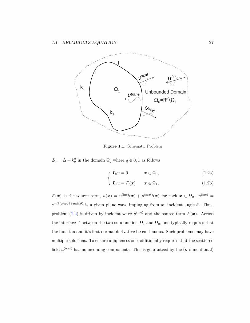
Consider an incident wave, u(inc), impinging on an arbitrary body Ω1, see Figure
1.1. It generates a transmitted wave, u(trans), and partially gets reflected, u(scat).
It could be an ultrasound wave scanning a kidney, an embryo, a carrier wave of a
cellular phone, a Wi-Fi radio signal passing through a wall or the head of a human.
In the frequency domain, such a scenario is described using the Helmholtz operator
1.1. HELMHOLTZ EQUATION 27
Г
k0
k1
Ω1
Ω0=Rn\Ω1
Unbounded Domain
Figure 1.1: Schematic Problem
Lq = ∆ + k2q in the domain Ωq where q ∈ 0, 1 as follows
L0u = 0 x ∈ Ω0, (1.2a)
L1u = F (x ) x ∈ Ω1, (1.2b)
F (x ) is the source term, u(x ) = u(inc)(x ) + u(scat)(x ) for each x ∈ Ω0. u(inc) =
e−ik(x cos θ+y sin θ) is a given plane wave impinging from an incident angle θ. Thus,
problem (1.2) is driven by incident wave u(inc) and the source term F (x ). Across
the interface Γ between the two subdomains, Ω1 and Ω0, one typically requires that
the function and it’s first normal derivative be continuous. Such problems may have
multiple solutions. To ensure uniqueness one additionally requires that the scattered
field u(scat) has no incoming components. This is guaranteed by the (n-dimentional)

28 CHAPTER 1. INTRODUCTION
Sommerfeld radiation condition:
∂u(scat)(x )
∂|x |+ ik0u
(scat)(x ) = o(|x |
1−n2
), as |x | → ∞. (1.3)
Problem (1.2) can be generalized for several bodies Ωqnq=1 ⊂ Ω0 which are
either mutually disjoint or share an interface. The problem is then defined as fol-
lowing:
L0u = 0 x ∈ Ω0,
L1u = F1(x ) x ∈ Ω1,
...
Lnu = Fn(x ) x ∈ Ωn,
(1.4)
driven by u(inc) and a set Fi, i = 1, 2, . . . , n. Across every interface one may require
that the function and it’s first normal derivative are continuous. One can also define
other interface conditions, those still can be handled by the method described below,
see equation (2.18). At infinity the Sommerfeld condition is required for uniqueness.
On the other hand, when one solves only an exterior (Ω0) or an interior (Ω1)
problem then only one boundary condition should be provided. For an exterior
problem, in addition to the Sommerfeld condition, one often requires that u(scat) =
−u(inc) or u(scat)n = −u(inc)
n on Γ which is the Dirichlet u|Γ = 0 and Neumann
un|Γ = 0 scattering problem, respectively. un, u(scat)n and u
(inc)n are the first normal
derivatives of u, u(scat), and u(inc) respectively.
Mathematical problems are often described better in some specific coordinate
system while in another system of coordinates the problem may have a less conve-

1.1. HELMHOLTZ EQUATION 29
nient representation. In boundary value problems one may change the coordinate
system to match the shape of the boundary, e.g. use polar coordinates for circular
domains or elliptical coordinates domains shaped as ellipses. However, when the
shape becomes more complicated the change of coordinates may become a major
difficulty. Furthermore, choosing a complicated coordinate system may lead to an
poor quality grid or singular points, thus ruining the advantage of changing coordi-
nates. Hence, there is a tradeoff between the complexity of the grid and complexity
of the problem.
For a generally shaped body, constructing a body fitted coordinate system needs
to be done numerically. Achieving this with high accuracy may be difficult. For a
complicated body, especially in 3D, it may be impossible to construct a simple body
fitted coordinate system. A partial remedy may be to use the multi-block overlap-
ping grids, also known as chimera grids, see, e.g., [30]. Those grids, however, do
not completely remove the difficulty associated with fitting the grid to a curvilinear
boundary. They rather partially alleviate it, because the grid no longer has to be
fitted to the entire boundary. Instead, different blocks serve different fragments of
the boundary, and instead of point matching, the grids are allowed to overlap on
some common regions, which simplifies their generation. Yet another alternative is
to use the finite element method based on an unstructured grid, see Section 1.2.
In this work we use a finite difference scheme with a regular grid regardless of
the shape of the body, and still obtain high order accuracy of the numerical solution.

30 CHAPTER 1. INTRODUCTION
1.1.1 Helmholtz equation in different coordinate systems
We next recast the Helmholtz equation two non-Cartesian coordinate systems. The
main difficulty is the Laplacian, which is defined as divergence of the vector gradient,
i.e. ∆u = div(gradu) ; one denotes div = ∇· and grad = ∇ to get ∆ = ∇ ·∇ = ∇2.
In the Cartesian coordinates one gets
∆ = ∇ ·(
∂
∂x1, . . . ,
∂
∂xn
)=
n∑j=1
∂2
∂x2j
.
Things are more complicated in polar coordinates, which are given as
x = r cos θ,
y = r sin θ,
where r ≥ 0 is a radius and 0 ≤ θ ≤ 2π is the angular coordinate. Using the chain
rule one gets
∂2
∂x2=
∂
∂x
(∂r
∂x
∂
∂r+∂θ
∂x
∂
∂θ
)=
∂
∂x
(cos θ
∂
∂r− sin θ
r
∂
∂θ
)= cos θ
∂
∂r
(cos θ
∂
∂r− sin θ
r
∂
∂θ
)− sin θ
r
∂
∂θ
(cos θ
∂
∂r− sin θ
r
∂
∂θ
)= cos θ
(cos θ
∂2
∂r2−(
sin θ
r
∂2
∂r∂θ− sin θ
r2
∂
∂θ
))− sin θ
r
(cos θ
∂2
∂θ∂r− sin θ
∂
∂r−(
sin θ
r
∂2
∂θ2+
cos θ
r
∂
∂θ
))

1.1. HELMHOLTZ EQUATION 31
and consequently
∂2
∂y2=
∂
∂y
(∂r
∂y
∂
∂r+∂θ
∂y
∂
∂θ
)=
∂
∂y
(sin θ
∂
∂r+
cos θ
r
∂
∂θ
)= sin θ
∂
∂r
(sin θ
∂
∂r+
cos θ
r
∂
∂θ
)+
cos θ
r
∂
∂θ
(sin θ
∂
∂r+
cos θ
r
∂
∂θ
)= sin θ
(sin θ
∂2
∂r2+
cos θ
r
(∂2
∂θ∂r− 1
r
∂
∂θ
))+
cos θ
r
(cos θ
(∂
∂r+
1
r
∂2
∂θ2
)+ sin
(∂2
∂r∂θ− 1
r
∂
∂θ
))
to arrive at the well known formulation
∆ =∂2
∂x2+
∂2
∂y2=
∂2
∂r2+
1
r
∂
∂r+
1
r2
∂2
∂θ2.
Such a complicated derivation is usually not convenient. Fortunately, bet-
ter methods exist. Consider an orthogonal curvilinear coordinate system y =
y(x ),x ∈ Rn. Define scale factors (also called metrics or Lame coefficients) as
h2j =
∑nm=1
(∂ym∂xj
)2. Then the vector gradient becomes ∇ =
(1h1
∂∂x1
, . . . , 1hn
∂∂xn
)and the Laplacian becomes
∆ =1∏n
j=1 hj
n∑m=1
∂
∂xm
(∏p 6=m hp
hm
∂
∂xm
).
Returning to polar coordinates one gets
hr =
√(∂x
∂r
)2
+
(∂y
∂r
)2
=√
cos2 θ + sin2 θ = 1,
hθ =
√(∂x
∂θ
)2
+
(∂y
∂θ
)2
=√r2 sin2 θ + r2 cos2 θ = r,

32 CHAPTER 1. INTRODUCTION
and the Laplacian is:
∆ =1
hrhθ
[∂
∂r
(hθhr
∂
∂r
)+
∂
∂θ
(hrhθ
∂
∂θ
)]=
1
r
[∂
∂r
(r∂
∂r
)+
∂
∂θ
(1
r
∂
∂θ
)]=
1
r
[∂
∂r+ r
∂2
∂r2+
1
r
∂2
∂θ2
]=
∂2
∂r2+
1
r
∂
∂r+
1
r2
∂2
∂θ2.
ϕ = 0
ϕ = π/6
ϕ = π/4
ϕ = π/3
ϕ = π/2
ϕ = 2π/3
ϕ = 3π/4
ϕ = 5π/6
ϕ = π
ϕ = 7π/6
ϕ = 5π/4
ϕ = 4π/3
ϕ = 3π/2
ϕ = 5π/3
ϕ = 7π/4
ϕ = 11π/6
η = 2
η = 2
η = 3/2
η = 3/2
η = 1
η = 1
(−d,0) (d,0)
Figure 1.2: Elliptical Coordinates
Elliptical coordinates are given by x+ iy = d cosh(η + iϕ) or, equivalently,
x = d cosh η cosϕ
y = d sinh η sinϕ
=
x = a cosϕ
y = b sinϕ
(1.5)
where d is semi-focal distance, η is an elliptical radius, so that each value of η defines
an unique ellipse with d =√a2 − b2, a = d cosh η, and b = d sinh η are the major
and minor semi-axes, respectively, and x2
a2+ y2
b2= cos2 ϕ+ sin2 ϕ = 1.

1.2. NUMERICAL APPROXIMATION OF DIFFERENTIAL EQUATIONS 33
In this case we have
hη = hϕ = d
√sinh2 η cos2 ϕ+ cosh2 η sin2 ϕ
= d
√sinh2 η cos2 ϕ+ cosh2 η(1− cos2 ϕ)
= d
√−(cosh2 η − sinh2 η) cos2 ϕ+ cosh2 η
= d
√cosh2 η − cos2 ϕ = d
√sinh2 η + sin2 ϕ
and consequently,
∆ =1
h2η
(∂2
∂η2+
∂2
∂ϕ2
).
1.2 Numerical approximation of differential equations
Finite difference (FD) methods were historically the first methodology for the nu-
merical solution of differential equations [54, 49]. They still remain a very powerful
tool, and for smooth solutions on regular grids lead to inexpensive and efficient algo-
rithms. Their primary disadvantage is in dealing with more complicated geometries
and solutions with low regularity. In particular, when the boundary is not aligned
with the grid staircase meshing doesn’t provide the required accuracy. For example,
consider a circular body Ω1 in Cartesian coordinates, see Figure 1.3. Denote the
circular boundary shape Γ = ∂Ω1 and let (x, y) ∈ Γ. Let vi,j be the approximate
value of the solution v at nodes xi = x + δx and yj = y + δy, i.e. vi,j ≈ v(xi, yj).
Let b(x, y) be the boundary value given on curve Γ and assume (xi, yj) /∈ Γ. The

34 CHAPTER 1. INTRODUCTION
Figure 1.3: Circular body in Cartesian coordinates, staircase-mesh γ.
staircase approach states vi,j = b(x, y). However, since
v(xi, yj) = b(x, y) +∇v(x, y) · (δx, δy) +O(δx2 + δy2),
and ∇v is not available, the boundary data is approximated by a first order method.
For additional discussion about staircase meshing and it’s disadvantages see [34].
The immersed boundary method (IBM) of Peskin [45] requires a modification of
the governing equations to treat the geometric irregularities, and a smoothed ap-
proximation of the δ function to treat the discontinuity at the interface, to achieve
first order accuracy. It has been improved upon with the immersed interface method
(IIM) of LeVeque and Li [37] (also see their book [38]). They enforce the jump at the
interface directly in the finite difference scheme. The implementation suffers from

1.2. NUMERICAL APPROXIMATION OF DIFFERENTIAL EQUATIONS 35
increased complexity, but second order accuracy can be achieved. Later Zhang and
LeVeque [71] used fictitious points to modify the discrete linear system to account
for the correct position of the interface and the proper physical interface condi-
tions. Recently Xu [68] developed efficient and stable boundary condition capturing
immersed interface method for simulating a flow around an object. The method
have almost a second order accuracy for the velocity and above first order for the
pressure. Johansen and Colella [36] used Embeded boundary to solve Poison equa-
tion with variable coefficients and Dirichlet boundary condition on irregular domain
using Cartesian grid with second order accuracy. They extended the solution into
a fictitious domain and the resultant linear system is non-symmetric. However it
is compatible with a multigrid and adaptive mesh techniques which should improve
the complexity. These techniques though aren’t immediately extendable for the
Helmholtz equation. Recently, Crockett, Colella and Graves [16] used this method
for Poison and heat equations with discontinuous coefficients and reached second
order. To the best of our knowledge, there are no reported uses in the literature of
those methods for anything but simple Dirichlet, Neumann, or interface conditions
(continuity of the solution and its normal flux), changing the boundary condition
requires major changes to the algorithm [16], and extension to higher than second
order accuracy is not straightforward. The ghost-cell immersed boundary method
(GCIBM) [62] employes extrapolation to impose the boundary condition implic-
itly; and the immersed boundary projection method (IBPM) [60] treats the no-slip
boundary conditions along with the immersed boundary as a Lagrange multiplier.
All these methods are difficult to generalize to high order accuracy.
A high order method (up to sixteenth-order accuracy) for elliptic equations, for

36 CHAPTER 1. INTRODUCTION
a matched interface and boundary method (MIB), was introduced by Zhou et al.
[74, 73]. The high-order interface conditions are implemented by repeatedly match-
ing the interface conditions across the given interface using low-order numerical in-
tegration rules. A special procedure is proposed to determine the accurate fictitious
values required for the high-order scheme. This method is meant to treat interface
curves that are not aligned to the grid, jumps in coefficients, and singular sources.
However, all the examples presented in [74, 73] reduce to a problem with only singu-
lar sources. Six new versions of IIM of fourth order accuracy were provided by Zhong
[72]. He used two different polynomials on both sides of the interface and enforced
that the two polynomials satisfy two interface conditions. Zhong used a wide stencil
that requires additional purely numerical boundary conditions. The only examples
provided were the Poisson equation with a singular source or equivalent.
An interesting solver was presented by Abarbanel and Ditkowski [1]. They con-
sidered a diffusion equation in one and two dimensions on a domain with a body
whose boundary points do not coincide with the nodes of a rectangular mesh. In
order to reach the fourth order accuracy, energy methods were used in conjunction
with simultaneous approximation terms (SAT). However, the resulting linear system
should be negative definite, which is not the case for the Helmholtz equation.
The finite element method (FEM) [58, 13, 7] and its extensions (GFEM, XFEM,
discontinuous enrichment [22, 23]), as well as discontinuous Galerkin methods [31],
are also well established and powerful. Their strength is in dealing with complex
geometries and low regularity of the solutions.
In practical problems of wave propagation though, especially in 3D, both FD

1.2. NUMERICAL APPROXIMATION OF DIFFERENTIAL EQUATIONS 37
and FEM have serious limitations because of their relatively high “points-per-
wavelength” requirement, as well as numerical dispersion and, more generally, nu-
merical pollution [35, Section 4.6.1], [5, 2]. The numerical phase velocity of the
wave in these methods depends on the wavenumber k, so a propagating packet of
waves with different frequencies gets distorted in the simulation. Furthermore, the
numerical error depends strongly on the wavenumber k, see [35], and this kind of
error is inherent in FEM/FD. The error behaves like hpkp+1 where p is the order of
accuracy of the scheme. So the number of points per wavelength needed for a given
accuracy grows like k1/p. Hence, for higher order accurate schemes the pollution
effect is reduced.
A high order approximation can be built for arbitrary boundaries using FEM,
but only in fairly sophisticated and costlier algorithms with isoparametric elements
[58]. In discontinuous enrichment / discontinuous Galerkin methods and GFEM,
high order accuracy also requires additional degrees of freedom, which entails an ad-
ditional computational cost. These additional degrees of freedom lead to expanded
approximating spaces which are capable of approximating a very broad class of
functions that may, in principle, have irregularities anywhere in the computational
domain. This is a significant advantage in problems of great geometrical and phys-
ical complexity. However, for simpler problems with smooth solutions much more
targeted and economical approximations, in narrower functional spaces, are available
using FD methods.
A FD approach, on the other hand, does not introduce additional unknowns per
grid node and thus remains inexpensive. It, however, requires a higher regularity
of the solution to guarantee consistency, and may also need a wider stencil, which

38 CHAPTER 1. INTRODUCTION
complicates the boundary conditions (more precisely, requires additional “purely
numerical” boundary conditions).
Schemes known as Collatz “Mehrstellen” [14], equation-based and related com-
pact schemes [55, 66, 69, 33, 3, 4, 8, 9], as well as Trefftz-FLAME [63], don’t expand
the stencil and therefore don’t require additional nonphysical boundary conditions.
Furthermore, as opposed to classical FEM which expands the approximating space,
these methods reduce it to the class of solutions rather than the much broader class
of generic sufficiently smooth functions. This does not imply any loss of generality,
because according to the Lax theorem, for convergence one does not need to have
consistency for any functions except the solutions.
1.2.1 Compact Equation–Based Schemes
We next present the compact scheme used hereafter in our simulations. Consider
ui,j = u (xi, yj), then the second order accurate approximation to the second deriva-
tive in x yields
Dxxui,j =ui+1,j − 2ui,j + ui−1,j
h2x
. (1.6)
Using Taylor series one can show that
Dxxui,j = uxx +h2x
12uxxxx +O
(h4).

1.2. NUMERICAL APPROXIMATION OF DIFFERENTIAL EQUATIONS 39
To obtain a 4th order approximation one eliminates uxxxx using the two dimensional
Helmholtz equation −uxx = uyy + k2u− F . Differentiating this equation we obtain
−uxxxx = uyyxx +(k2u)xx− Fxx = DyyDxxu+Dxx
(k2u− F
)+O(h2)
where Dyyui,j =ui,j+1−2ui,j+ui,j−1
h2y. Thus, the fourth order compact scheme is given
by
Dxxui,j = Dxxui,j −h2x
12
(DyyDxxu+Dxx
(k2u− F
))= uxx +O
(h4). (1.7)
Using a similar approach for the derivative in y, one gets the scheme of Singer and
Turkel [55]
(Dxx +Dyy + k2 +
1
12
(h2x + h2
y
)DxxDyy
)u+
1
12
(h2xDxx + h2
yDyy
) (k2u)
=
(1 +
1
12
(h2xDxx + h2
yDyy
))F. (1.8)
Compact fourth order accurate schemes for the more general Helmholtz -type
equations with variable coefficients have been obtained in [8, 9]. A sixth order
scheme for constant coefficients is constructed in [56]. A similar compact sixth
order scheme for the case of a variable wavenumber k = k(x ) is presented in [65].
A distinctive feature of the compact equation-based schemes is that they exploit
two stencils. The first one applies to the left-hand side of the equation, i.e., it
operates on the unknown solution. The second one applies to the right-hand side of

40 CHAPTER 1. INTRODUCTION
the equation, i.e. , it operates on the given data (source terms). The equation-based
and similar high order schemes reduce pollution while keeping the treatment of the
boundary conditions simple. Since the order of the resulting difference equation is
equal to the order of the differential equation, no nonphysical boundary conditions
are required.
1.2.2 Reduction to integral equations
In traditional boundary element methods (BEM), linear boundary value problems
are transformed into integral equations with respect to equivalent boundary sources,
which are subsequently discretized. Practical applications of such methods date
back to the 1960s. They impose no limitations on the shape of the boundary and
automatically account for the correct far field behavior. There are, however, several
major disadvantages:
• Full matrices — in contrast with the sparse FD and FEM matrices. (Cases of
quasi-sparse integral equations, due to the rapid decay of Green’s functions in
space, are exceptional, [46]).
• A relatively narrow treatment of the boundary conditions. Care must be exer-
cised, on a case-by-case basis, in the choice of the equivalent boundary sources,
so that the resulting Fredholm equation is of the second kind (well-posed)
rather than first. Moreover, mixed (Dirichlet/Neumann, etc.) or less standard
(Robin, etc.) conditions require a special development.
• Singular integral kernels (the most serious disadvantage in practice). Imme-

1.2. NUMERICAL APPROXIMATION OF DIFFERENTIAL EQUATIONS 41
diately at the boundary points, the kernel singularity can usually be handled
analytically, and the fields remain bounded as long as the surfaces are smooth.
However, for points in the vicinity of a surface, the evaluation of the integral
is problematic, as analytical expressions are usually unavailable and numerical
quadratures require extreme care.
• Limitation to constant coefficients, i.e., to homogeneous media, — these meth-
ods require explicit knowledge of the fundamental solution of the correspond-
ing differential operator.
Significant progress in Fast Multipole Methods (FMM) [25, 12, 40, 70, 24] has
helped alleviate the first disadvantage of boundary methods. FMM accelerates the
computation of fields due to distributed sources — or equivalently, matrix-vector
multiplications for the dense system matrices. But the second and especially the
third disadvantages are more difficult to overcome, whereas the fourth one can only
be addressed by switching to much less efficient volume integral methods or finding
the fundamental solution by numerical means, which is both expensive and leads to
additional errors.

42 CHAPTER 1. INTRODUCTION

Chapter 2
Problems with non-aligned
interfaces
In this chapter we describe our main methodological approach for solving problem
(1.2). We consider a divide and conquer approach based on wave splitting into
incoming and outgoing waves. We assemble the overall solution from the set of
individual solutions to the auxiliary problem (AP). The AP is defined independently
for each sub-domain Ωq, see (1.2). The choice of the AP is relatively flexible; it can
be formulated so as to enable an easy and economical numerical solution. Our new
method uses only simple structured grids, e.g., Cartesian or polar, regardless of
the shape of the boundaries or interfaces. In the regions of smoothness, it employs
high order accurate finite difference schemes on compact stencils, see Section 1.2.1.
They do not require any additional boundary conditions besides those needed for
the underlying differential equation itself.
43

44 CHAPTER 2. PROBLEMS WITH NON-ALIGNED INTERFACES
We first illustrate the key components of the numerical methodology that we
propose with a one dimensional example and then generalize this simple one di-
mensional model of wave splitting into a multidimensional one using Calderon’s
projections, see [39].
Consider the following one-dimensional problem
uxx + k20u = 0 x < 0,
uxx + k21u = 0 x > 0,
(2.1)
driven by an incoming wave u(inc) = Aeik0x, which propagates through the domain.
It generates the transmitted wave u1 = Teik1x for x > 0 and partially gets reflected
and produces u0 = Re−ik0x for x < 0, see Figure 2.1.
x=0
Aik x
e
ik xeT
R−ik x0
1
e 0
Figure 2.1: 1D transmission problem.

45
To find the amplitudes T and R one requires that u(x) and u′(x) be continuous at
x = 0. This yields two linear algebraic equations: A+R = T and k0A−k0R = k1T ,
which provide the Fresnel reflection and transmission coefficients:
T = A2k0
k0 + k1, R = A
k0 − k1
k0 + k1. (2.2)
However, one can solve this problem without introducing unknown amplitudes
and instead employ the relation that describes the entire family of waves: right
traveling u′− ik1u = 0 and the left traveling u′+ ik0u = 0. In particular, the trans-
mitted wave u1 satisfies the right traveling equation. Likewise u0 + u(inc) satisfies
the inhomogeneous left traveling equation on x < 0. So we can rewrite (2.1) as the
following system of equations
u′ − ik1u = 0 x > 0,
u′ + ik0u = 2ik0Aeik0x x < 0,
(2.3)
together with the requirement that u(x), u′(x) be continuous, which yields:
u(0) = A2k0
k0 + k1, u′(0) = A
2ik1k0
k0 + k1. (2.4)
Since T =A+R=u(0), we arrive at the same answer (2.2).
The system of equations (2.3) shows that if the impinging wave changes (new
amplitude A), then the problem does not have to be solved all over again, because
only the right-hand side of inhomogeneous part changes. In one dimension the
difference is negligible. However, in multiple space dimensions a methodology built

46 CHAPTER 2. PROBLEMS WITH NON-ALIGNED INTERFACES
around the same idea proves very useful. For example, in inverse problems one may
cheaply use multiple impinging waves or different incident angles to get additional
information to improve the accuracy.
In Section 2.1 we present the theoretical part for Calderon’s boundary equations
with projections which replaces the system of equations (2.3). We conclude chap-
ter Chapter 2 describing the discrete counterparts of the boundary equations with
projections developed by V.S. Ryaben’kii, see [50], in Section 2.3. The pseudocode
of the main algorithm for solving (1.2) is described in Section 2.3.1, followed by
examples and additional explanation in Sections 2.3.2 – 2.3.7.
2.1 Calderon’s Potentials
In this section we present the Calderon potentials, which yield the wave splitting
described above, see [39]. All the incoming and outgoing waves for a given Ωq
(analogues of the right and left traveling waves in 1D example, see Figure 2.1) belong
to the image (range) and kernel (null space), respectively, of the corresponding
projection operator. We consider time-harmonic wave propagation with a piecewise
continuous index of refraction.
Let Lq denote the Helmholtz operator of equation (1.1) with k = kq, where
q ∈ 0, 1, and the geometry as depicted in Figure 1.1, i.e. we consider problem (1.2).
Let Gq(x ) be the fundamental solution of Lq. Let the functions ξI(x ) and ξII(x )
belong to C2 , C1 respectively for x ∈ Γ. We introduce the vector ξξξΓ = (ξI , ξII)
which we call the vector density. A generalized potential of Calderon type with the

2.1. CALDERON’S POTENTIALS 47
vector density ξξξΓ is defined by
PΩqξξξΓ(x ) = σq
∫Γ
(ξI(y)
∂Gq∂n
(x− y)− ξII(y)Gq(x− y)
)dsy , x ∈ Ωq, (2.5)
where ∂∂n denotes the normal derivative and σq = (−1)q+1 changes the sign so that
we always consider a normal pointing in the same direction regardless of the domain
Ωq. Given the solution u(x ) to the problem (1.2) one defines a vector density
uΓ =(u, ∂u∂n
)∣∣Γ, and rewrites Green’s solution to the problem (1.2) as:
u(x ) =
PΩ1uΓ +
∫Ω1G1(x − y)F (y)dy x ∈ Ω1,
PΩ0uΓ x ∈ Ω0.
(2.6)
Let ξξξΓ = (ξI , ξII) belong to the space S . Inspired by the one dimensional
example we wish to split S into incoming S q+ and outgoing S q
− waves for a given Ωq
such that their direct sum is S , i.e.
S = S q+ ⊕ S q
−. (2.7)
So for each ξξξΓ ∈ S we looking for ξξξ+Γ ∈ S
q+ and ξξξ−Γ ∈ S
q− such that ξξξΓ = ξξξ+
Γ + ξξξ−Γ .
Furthermore, we require that such a representation be unique. One implements it
by a projection operator whose image is Sq+ and it’s kernel is Sq−. We stress that
while the space S doesn’t change, the representation (2.7) changes for the exterior or
interior problem, e.g. S1+ 6= S0
− in general. In addition, the choice of the projection
operator affects the representation of (2.7), which can be considered as changing
the projection angle onto the same subspace [39].

48 CHAPTER 2. PROBLEMS WITH NON-ALIGNED INTERFACES
One defines such a projection operator using Calderon’s potential (2.5). This
projection is known as the Calderon’s boundary projection. We will show that this
projection implies a wave split, see discussion in Section 2.1.1. We first define the
vector trace operator Tr v =(v, ∂v∂n
)∣∣Γ. Thus, Calderon’s boundary projection is
defined as
PqΓξξξΓ = Tr PΩqξξξΓ. (2.8)
Note, that any ξξξΓ satisfies LqPΩqξξξΓ = 0, x ∈ Ωq, and therefore Green’s formula
provides PΩqξξξΓ = PΩqTr PΩqξξξΓ which immediately implies that PqΓ is a projection
since (PqΓ)2 = Pq
Γ.
The operator PqΓ has an important property. If ξξξΓ defines u(x) = PΩqξξξΓ for
which Tr u(x) = ξξξΓ , then the following equation holds
PqΓξξξΓ = ξξξΓ. (2.9)
If equation (2.9) holds, then u(x) = PΩqξξξΓ satisfies Lqu = 0, and Tr u = ξξξΓ.
Finally, we have proved that ξξξΓ satisfies the BEP if and only if ξξξΓ = Tr u for which
Lq u = 0 [51, 53, 39]. We call equation (2.9) the boundary equation with projection
(BEP).
2.1.1 Wave Split
The solutions to the homogeneous equation Lqu = 0 can be interpreted as incoming
waves for the domain Ωq, because they have no (radiating) sources on Ωq. In order
to describe how Calderon’s projection splits the waves [39], we first recast equation

2.1. CALDERON’S POTENTIALS 49
(2.5) as:
PΩqξξξΓ(x ) =
σq∫
Γ
(ξI(y)
∂Gq
∂n (x − y)− ξII(y)Gq(x − y))dsy , x ∈ Ωq,
0 x ∈ Rn \ Ωq.
(2.10)
Next we define Green’s operator on Lq as
GqF (x ) =
∫
ΩqGq(x − y)F (y)dy , x ∈ Ωq,
0 x ∈ Rn \ Ωq.
(2.11)
Thus, one expresses the exterior solution as u0(x ) = PΩ0u0Γ(x ) where
u0Γ = Tr u0 =
(u0,
∂u0
∂n
)∣∣∣∣Γ
,
and the interior solution as the u1(x ) + G1 F (x ) = PΩ1u1Γ(x ) + G1 F (x ) where
u1Γ = Tr u1 =
(u1,
∂u1
∂n
)∣∣∣∣Γ
.
Hence, the solution to the problem (1.2) is given by
u(x ) = u0(x ) + u1(x ) + G1 F (x ), x ∈ Rn. (2.12)
We next denote uΓ = u1Γ + u0
Γ. Note, that in general uΓ does not satisfy the
BEP unless uΓ = uqΓ. This means that the operator PqΓξξξΓ eliminates that part of ξξξΓ
which is not the trace of the solution of Lqu = 0. In other words incoming waves to
Ωq, denoted as ξξξ+Γ , belong to the image of the projection Pq
Γ, i.e. ξξξ+Γ ∈ ImPq
Γ while

50 CHAPTER 2. PROBLEMS WITH NON-ALIGNED INTERFACES
outgoing waves to Ωq satisfy ξξξ−Γ ∈ KerPqΓ. Therefore, the aforementioned space S
satisfies S = ImPqΓ ⊕KerPq
Γ, since Sj+ = ImPqΓ and Sj− = KerPq
Γ.
The operators P qΓ are defined in such a way so that if there is no discontinuity,
i.e. k0 = k1 then ImP1Γ = KerP0
Γ and KerP1Γ = ImP0
Γ, and so there are no reflections
at Γ. However, in general ImP1Γ 6= KerP0
Γ and KerP1Γ 6= ImP0
Γ, which means that
there is both propagation through and reflection from the interface Γ, similar to the
1D case, see Figure 2.1.
2.1.2 Reduction of the problem to the boundary
For an exterior domain Ω0 the solution is u = u+u(inc) where u denotes the scattered
field satisfying the Sommerfeld radiation condition (1.3). Therefore, due to the
linearity of the trace operator, the density ξξξΓ for the exterior domain is given by
ξξξΓ = Tru = Tr u+ Tru(inc) = ξξξΓ + ξξξ(inc)Γ .
To satisfy (1.3) one formulates the BEP for the exterior problem for the scattered
field:
P0Γ ξξξΓ = ξξξΓ.
However, in order to match it to the interior part one complements it, for the total
field, by adding P0Γ ξξξ
(inc)Γ + ξξξ
(inc)Γ to both sides of the equation. Hence, assuming
that the solution and its first normal derivative are continuous across Γ, we can
equivalently reformulate problem (1.2) as the following system of BEP [53] defined
on ξξξΓ:

2.1. CALDERON’S POTENTIALS 51
P1
Γ ξξξΓ + TrG1F = ξξξΓ,
P0Γ ξξξΓ + (I −P0
Γ)ξξξ(inc)Γ = ξξξΓ.
(2.13)
System (2.13) can be thought of as a multi-dimensional analogue of system (2.3).
Once (2.13) has been solved for ξΓ, the solution u(x) is given by
u(x ) =
PΩ1ξξξΓ(x ) + G1F (x ) x ∈ Ω1,
PΩ0 [ξξξΓ − ξξξ(inc)Γ ](x ) + u(inc)(x ) x ∈ Ω0.
(2.14)
Note that the application of the trace operator Tr reduces system (2.14) back to
(2.13).
2.1.3 Divide and Conquer
One of the important generalizations of the proposed method is that one can redefine
(2.13) in such a way so that it is possible to solve it as two separate auxiliary prob-
lems (AP) one for the interior and one for the exterior domain. Such an approach
has several advantages. For example, one can solve each of the auxiliary problems
on a different grid. Another example is that one can change the Sommerfeld approx-
imation without recalculating the auxiliary problem for the interior area. However,
the main advantage is the relatively simple treatment of curvilinear interfaces Γ as
will be explained in the next section.
Consider an arbitrary function w(x ), x ∈ Rn, that satisfies the Sommerfeld
radiation condition (1.3) and such that Trw = ξξξΓ = (ξI , ξII). Generally Lqw 6= 0,

52 CHAPTER 2. PROBLEMS WITH NON-ALIGNED INTERFACES
x ∈ Ωq, and therefore Green’s formula gives:
w(x ) = PΩq wΓ + Gq Lq w, x ∈ Ωq.
Using the fact that PΩq wΓ = PΩq ξξξΓ(x ), we get
PΩq ξξξΓ(x ) = w(x )−GqLqw, x ∈ Ωq. (2.15)
We next generalize (2.15) in the following way: let Lq be defined for x ∈ Rn
(instead of x ∈ Ωq). We reformulate PΩq so that the equation (2.5) becomes
PΩq ξξξΓ(x ) = w(x )−Gq
(Lqw)
∣∣Ωq
, x ∈ Ωq. (2.16)
The potential (2.16) is obtained on Rn and then restricted to Ωq. Furthermore, it
is insensitive to the choice of w as long as the conditions Trw = ξξξΓ and (1.3) hold.
The projection PqΓ defined through (2.16) is the same as one defined through (2.5).
The importance of this new definition is that it does not contain surface integrals.
This further generalization is the key feature in the treatment of generally shaped
bodies that are not aligned to the numerical grid, which is discussed in Section 2.3.
Let Ωq be a regularly shaped expanded domain such that Ωq ⊂ Ωq. Assume that Lq
is also defined on Ωq, and that Gq is the corresponding inverse so that the solution u
to the equation Lqu = F on Ωq is given by u = GqF . Hereafter, we assume that this
solution exists for any given F defined on Ωq and is unique as along as u is required
to satisfy some specially chosen boundary conditions at ∂Ωq. The combination of
the differential equation Lqu = F and these boundary conditions will be referred to

2.1. CALDERON’S POTENTIALS 53
as the auxiliary problem (AP). The AP can be constructed so that it is easy to solve.
In particular, the evaluation of GqF does not need to involve any singular integrals.
Instead, the AP is discretized, and its solution computed using finite differences on
a regular grid (see Section 2.3). Finally, problem (1.2) is solved as two different
BEPs defined on ξξξΓ: P1
Γ ξξξ1Γ + TrG1F = ξξξ1
Γ,
P0Γ ξξξ
0Γ + (I −P0
Γ)ξξξ(inc)Γ = ξξξ0
Γ,
(2.17)
subject to the condition
Aξξξ1Γ + Bξξξ0
Γ = 0 , (2.18)
which is an additional generalization to (2.13) where A = B = 1. This last gener-
alization is the pathway for different interface conditions.
We denote ξξξqΓ = (ξIq , ξIIq ) where q ∈ 0, 1 refers to the interior or exterior traces
in (2.17). ξIq , ξIIq are the solution and it’s normal derivative on the interface Γ,
and are therefore unknown. In order to solve system (2.17) one expands both ξξξ1Γ,
ξξξ0Γ in some basis, e.g. Fourier, so that the coefficients of the expansion become the
unknowns of the problem. Once the coefficients are known and ξξξ1Γ, ξξξ0
Γ assembled,
the solution is computed by (2.14). We describe this approach in more detail and
provide examples in Section 2.3.
54 CHAPTER 2. PROBLEMS WITH NON-ALIGNED INTERFACES
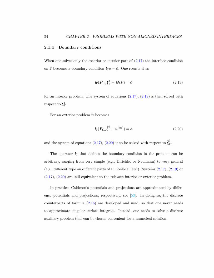
2.1.4 Boundary conditions
When one solves only the exterior or interior part of (2.17) the interface condition
on Γ becomes a boundary condition lΓu = φ. One recasts it as
lΓ(PΩ1 ξξξ1Γ + G1F ) = φ (2.19)
for an interior problem. The system of equations (2.17), (2.19) is then solved with
respect to ξξξ1Γ.
For an exterior problem it becomes
lΓ(PΩ0 ξξξ0
Γ + u(inc)) = φ (2.20)
and the system of equations (2.17), (2.20) is to be solved with respect to ξξξ0
Γ.
The operator lΓ that defines the boundary condition in the problem can be
arbitrary, ranging from very simple (e.g., Dirichlet or Neumann) to very general
(e.g., different type on different parts of Γ, nonlocal, etc.). Systems (2.17), (2.19) or
(2.17), (2.20) are still equivalent to the relevant interior or exterior problem.
In practice, Calderon’s potentials and projections are approximated by differ-
ence potentials and projections, respectively, see [53]. In doing so, the discrete
counterparts of formula (2.16) are developed and used, so that one never needs
to approximate singular surface integrals. Instead, one needs to solve a discrete
auxiliary problem that can be chosen convenient for a numerical solution.

2.2. WELL-POSEDNESS 55
2.2 Well-posedness
We assume that the original problem (1.2) is well-posed, i.e., that its solution exists,
is unique, and depends continuously on the data F (x ), φ, in the sense of appropri-
ately chosen norms. Then, the equivalent problem on the interface (2.17), (2.18)
or on the boundary (2.17), (2.19) or (2.17), (2.20) is also well-posed. This means
that if the BEP is perturbed, then the solution of the boundary system will also get
perturbed, and the perturbation of the solution will be bounded in the appropriate
norm by the perturbation introduced into the BEP.
For instance, consider the interior homogeneous case:
Lu = 0 on Ω and lΓu = φ on Γ,
for which the equivalent boundary formulation is
PΓξξξΓ − ξξξΓ = 0 and lΓ(PΩξξξΓ) = φ.
If the original problem is well-posed, then ‖u‖ 6 c‖φ‖, and consequently,
‖ξξξΓ‖ 6 c1‖φ‖.
This result has nothing to do with Calderon’s operators per se, it holds simply
because ξξξΓ = Tru. LetψψψΓ be a perturbation, so that instead of the true unperturbed
boundary problem we are solving
PΓξξξΓ − ξξξΓ = ψψψΓ and lΓ(PΩξξξΓ) = φ.

56 CHAPTER 2. PROBLEMS WITH NON-ALIGNED INTERFACES
Then, we have
‖ξξξΓ‖ 6 C(‖φ‖+ ‖ψψψΓ‖),
where the constant C depends on ‖PΩ‖ and ‖PΓ‖, but does not depend on either
φ or ψψψΓ. The proof can be found in [52, Part II, Chapter 1]. It is based on splitting
the entire space of traces ξξξΓ on Γ into the direct sum: ImP jΓ ⊕KerP j
Γ as discussed
above.
2.3 Discrete Calderon’s Potentials
We now develop the discrete counterpart of the theory introduced in the previous
section. To make the presentation easier we first describe it in relatively simple
algorithmic terms in Section 2.3.1 followed by several representative problems and
their solution supported by BEP theory in mathematical and algorithmic terms in
following sections. We stress, despite the fact that we only provide examples with
simple regular shapes, the theory remains unchanged for a generally shaped body.
2.3.1 Algorithm
In this section we present a sequence of simple algorithmic steps that implements
the solution of problem (1.2).
Thus, we provide pseudocode of the main procedures required to implement our
method and give several algorithms for solving the problem in a domain not aligned
to the grid including the transmission-reflection algorithm in heterogeneous media
with a jump at the interface and an efficient algorithm for multiple impinging waves.

2.3. DISCRETE CALDERON’S POTENTIALS 57
The main advantage of our method is that for each sub-domain Ωq, see (1.2), we
compute a relatively small set of individual solutions to a simple auxiliary problem
on a regular domain formulated to be numerically effective. Individual solutions are
used to assemble the solution of the original problem.
More precisely, we solve the system of BEPs (2.17), (2.18) as follows. For each
BEP, exterior (q = 0) or interior (q = 1) we consider an expansion of ξξξqΓ = (ξIq , ξIIq )
in some basis on Γ, e.g. Fourier:
ξIq (s) =∑
cI,qn bn(s), (2.21a)
and
ξIIq (s) =∑
cII,qn bn(s), (2.21b)
so that the problem is reduced to finding the coefficients cI,qn , cII,qn that satisfy the
condition
A(∑
cI,0n bn(s),∑
cII,0n bn(s))
+ B(∑
cI,1n bn(s),∑
cII,1n bn(s))
= 0 (2.22)
obtained by substituting expressions (2.21) into formula (2.18). Each individual
solution corresponds to a basis function chosen on Γ and extended to it’s grid rep-
resentation γ by means of the operator T to be defined in Section 2.3.1.2.
In the following sections we define γ, then describe the extension of basis func-
tion, and then describe and provide pseudocode of the discrete counterpart of
Calderon’s potentials theory followed by examples of solutions to several problems.

58 CHAPTER 2. PROBLEMS WITH NON-ALIGNED INTERFACES
2.3.1.1 The grid representation of the boundary shape
pi-1,j-1
pi,j
pi+1,j+1
pi,j+1
pi-1,j+1
pi+1,j
pi-1,j
pi,j-1
pi+1,j-1
Figure 2.2: 9-point stencil centered at node pi,j
We define now the grid representation of the curve Γ, which we denote γ, in a
following way. Let Ω be a smooth body in the domain represented by regular grid
N, e.g. Cartesian. Since Ωq is not necessary aligned to the grid, the intersections
between N and Γ may be an empty set, therefore we define γ to be a set of grid
points surrounding Γ. Formally, let Npi,j be the stencil centered at node pi,j , e.g.
the 9-point stencil on Figure 2.2 and let N+,N− be non-empty sets defined as
N+ =⋃
pi,j∈Ωq
Npi,j , N− =⋃
pi,j∈N\Ωq
Npi,j ,
where q ∈ 0, 1. Then the grid representation of the curve Γ, γ, is given as
γ = N+ ∩ N−. (2.23)
An example of γ for general body in Cartesian coordinates is shown in Figure 2.3.
In Figure 2.4 we present γ for a similar general body in polar coordinates.

2.3. DISCRETE CALDERON’S POTENTIALS 59
Figure 2.3: Example of γ: general body in Cartesian coordinates.
2.3.1.2 Extension of the basis function
We next define a new scalar function ξξξqγ in the vicinity of Γ which represents the
numerical counterpart of the trace of the solution ξξξqΓ. ξξξqγ is obtained by extension
of ξξξqΓ from Γ to γ using Equation-Based extension. The idea behind Equation-
Based extension is similar to the approach used to construct compact schemes (see
Section 1.2.1). Given the function and the first normal derivative contained in ξξξqΓ,
one differentiates the Helmholtz equation Lq u = F to obtain higher order normal
derivatives and uses these to build a Taylor formula (2.24) that yields the value of

60 CHAPTER 2. PROBLEMS WITH NON-ALIGNED INTERFACES
Figure 2.4: Example of γ: general body in polar coordinates.
ξξξqγ at every node γ.
v(n+ δn, s) = v(n, s) +N∑t=1
1
t!
∂tv(n, s)
∂ntδnt (2.24)
We denote the Equation-Based Taylor extension as ξξξqγ = T (ξIq , ξIIq , F |Γ) where F
is the source term of the equation. An example of Equation-Based Taylor extension
in polar coordinates can be found in Section 2.3.2 and in Section 2.3.5 we show the
extension in elliptic coordinates. The general case is analyzed in [42].
The extension T applies to any boundary vector function ξξξΓ = (ξIq , ξIIq ), and
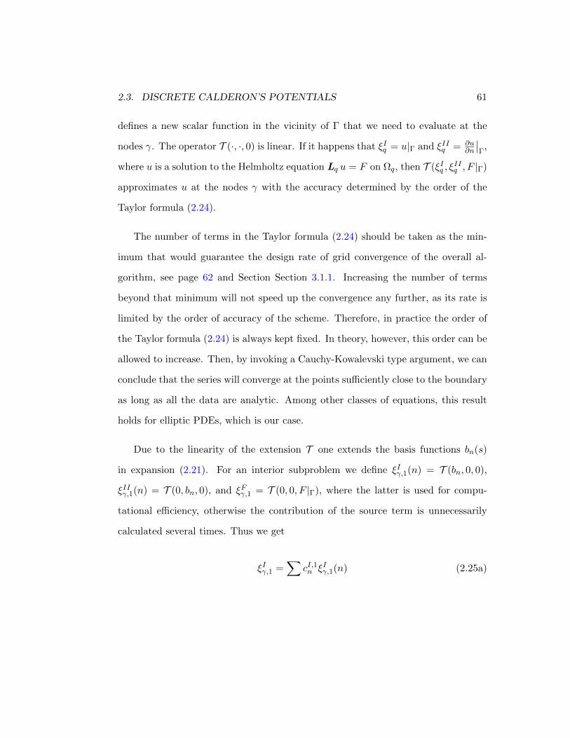
2.3. DISCRETE CALDERON’S POTENTIALS 61
defines a new scalar function in the vicinity of Γ that we need to evaluate at the
nodes γ. The operator T (·, ·, 0) is linear. If it happens that ξIq = u|Γ and ξIIq = ∂u∂n
∣∣Γ,
where u is a solution to the Helmholtz equation Lq u = F on Ωq, then T (ξIq , ξIIq , F |Γ)
approximates u at the nodes γ with the accuracy determined by the order of the
Taylor formula (2.24).
The number of terms in the Taylor formula (2.24) should be taken as the min-
imum that would guarantee the design rate of grid convergence of the overall al-
gorithm, see page 62 and Section Section 3.1.1. Increasing the number of terms
beyond that minimum will not speed up the convergence any further, as its rate is
limited by the order of accuracy of the scheme. Therefore, in practice the order of
the Taylor formula (2.24) is always kept fixed. In theory, however, this order can be
allowed to increase. Then, by invoking a Cauchy-Kowalevski type argument, we can
conclude that the series will converge at the points sufficiently close to the boundary
as long as all the data are analytic. Among other classes of equations, this result
holds for elliptic PDEs, which is our case.
Due to the linearity of the extension T one extends the basis functions bn(s)
in expansion (2.21). For an interior subproblem we define ξIγ,1(n) = T (bn, 0, 0),
ξIIγ,1(n) = T (0, bn, 0), and ξFγ,1 = T (0, 0, F |Γ), where the latter is used for compu-
tational efficiency, otherwise the contribution of the source term is unnecessarily
calculated several times. Thus we get
ξIγ,1 =∑
cI,1n ξIγ,1(n) (2.25a)

62 CHAPTER 2. PROBLEMS WITH NON-ALIGNED INTERFACES
and
ξIIγ,1 =∑
cII,1n ξIIγ,1(n), (2.25b)
and we define
ξξξ1γ = ξIγ,1 + ξIIγ,1 + ξFγ,1. (2.26)
For an exterior (homogeneous) subproblem we define ξIγ,0(n) = T (bn, 0, 0) and
ξIIγ,0(n) = T (0, bn, 0), thus
ξIγ,0 =∑
cI,0n ξIγ,0(n) (2.27a)
and
ξIIγ,0 =∑
cII,0n ξIIγ,0(n), (2.27b)
and we define
ξξξ0γ = ξIγ,0 + ξIIγ,0. (2.28)
Theoretically, to reach nth order of accuracy for the overall solution to the prob-
lem one requires N = n+ 2, see [47]. However the experimental results presented in
Section 3.1.1 and in [42] show that it is sufficient to take N = n.
We should also mention that according to [28, 27, 59], for maintaining the overall
given order of accuracy across the domain, it may be sufficient to approximate the
boundary conditions with lower accuracy. In the future, it may be of interest to
investigate whether this phenomenon is related to our finding that the order of the
extension operator can be taken lower than theoretically predicted.

2.3. DISCRETE CALDERON’S POTENTIALS 63
2.3.1.3 Difference Potentials
In section Section 2.1.3 we required an arbitrary function w(x ), x ∈ Rn, that satisfies
the Sommerfeld radiation condition (1.3) and such that it’s vector trace is equal ξξξΓ,
i.e. Trw = (w,wn) = (ξI , ξII) = ξξξΓ where wn is the normal derivative of w along
Γ. We denote the discrete trace operator similarly as the continuous one, i.e. Tr .
In the discrete case the trace operator become the value of the function at the grid
boundary γ, i.e. Trw = w|γ . Thus, we require the discrete w to satisfy Trw = ξξξγ ,
where ξξξγ defined in Section 2.3.1.2.
Numerically one creates w(x ) using the same structure and the same size as the
solution to the problem. One fills w(x ) with values of ξγ at nodes corresponding to
γ and zeroes elsewhere. We present such a procedure in Algorithm 1:
Algorithm 1 Create w from ξγ
function W(ξγ)w ← 0 on grid Nw|γ ← ξγreturn w
end function
Let S(N, k, F, g) be a solver of the equation (1.1) on some regular grid N subject
to the numerical boundary condition u|∂N = g, where ∂N is the informal notation
for boundary nodes of N. We seek to solve the same AP with different source terms.
Therefore, we choose a fixed g to provide uniqueness and redefine the solver as
S(N, k, F ). Let n be the order of accuracy of S. One can use the solver described
in Section 1.2.1 or as described in more detail in [65, 42, 10, 55, 41]. We denote by
S the solver for either the exterior or interior problem.
We next define, in Algorithm 2, the discrete counterpart of Calderon’s potential

64 CHAPTER 2. PROBLEMS WITH NON-ALIGNED INTERFACES
PΩq which, unlike in continues case, will take as input w(x ) instead of ξγ (see Section
2.1.3) and assume that Trw = ξξξγ or similarly w(x )|γ = ξγ , i.e. here we consider
w(x ) is known:
Algorithm 2 Calderon Potential PΩqξγ
function PΩq(N,k,w) . Assuming Trw = ξξξγ
rhs← 0 on grid Nrhs|Ωq ← (Lq w)|Ωq . set an artificial rhsv ← S(N, k, rhs)return w − v . return potential, see sections 2.1,2.3
end function
(Lq w)|Ωq is the result of the direct Helmholtz operator Lq on the entire grid N and
truncated to the domain of interest Ωq.
One defines Calderon Potential in the following way. Let u(s) = h(s) and
∂u∂n (s) = g(s) therefore:
Algorithm 3 Another definition of Calderon Potential
function PΩq(N,k,h,g,F )
ξγ ← T (h, g, F )w ←W(ξγ)return PΩq (N, k, w)
end function
The difference between Algorithm 2 and Algorithm 3 is that the latter creates w from
u and ∂u∂n using an extension T while the former gets w as an argument. Algorithm
2 can be used more effectively for multiple values of w, therefore Algorithm 3 is not
used in further algorithms and presented here for didactic purpose only.
We now define the projection operator, which numerically become a truncation
of the Calderon operator in Algorithm 4.

2.3. DISCRETE CALDERON’S POTENTIALS 65
Algorithm 4 Projection operator
function P qγ (N,k,ξγ)w ←W(ξγ)return PΩq
(N, k, w)|γend function
2.3.1.4 Examples of solutions to different problems
We next solve the homogeneous problem Lqu + k2qu = 0 in a domain Ωq (either
interior or exterior) and let the boundary condition bc of type bc type be given on
∂Ωq. We assume that the solution has an expansion in some functional basis, e.g.
Fourier, u(s) =∑
n c1nbn(s) and ∂u
∂n (s) =∑
n c2nbn(s) and get
Algorithm 5 The Solver for a homogeneous problem
function Homogeneous-SolverΩq(N,k,bc type,bc)
(ξIγ , QI , ξIIγ , QII)← BEPq(N, k) . See Algorithm 6
(cI , cII)← Coefficients(QI , QII , bc type, bc, 0) . See Algorithm 7u← 0 on grid Nu|Ωq
← (Sq(N, k, ξIγcI + ξIIγ cII))|Ωq
return uend function
Algorithm 6 used in Algorithm 5 plays the discrete counterpart of (2.9) which
one recasts as Pqγξξξγ = ξξξγ . The algorithm Algorithm 6 doesn’t provide the solution
to BEP, but the matrix with columns of (P qγ −I)ξγ(n) where ξγ(n) denotes nth basis
function extended to the γ, see Section 2.3.1.2. This matrix is used to construct the
linear system which is solved to find the coefficients of the expansion (2.21).

66 CHAPTER 2. PROBLEMS WITH NON-ALIGNED INTERFACES
Algorithm 6 BEP
function BEPq(N,k) . Calculate operator (P qγ − I)ξγforeach Basis Functions bn
ξIγ(n)← T (bn, 0, 0) . set ξγ ’s as columns of matrices ξIγ , ξIIγ
ξIIγ (n)← T (0, bn, 0)
5: PI(n)← P qγ (N, k, ξIγ(n)) . solutions to AP’s are columns of PI , PIIPII(n)← P qγ (N, k, ξIIγ (n))
end foreach
QI ← PI − ξIγQII ← PII − ξIIγ
10: return (ξIγ , QI , ξIIγ , QII)
end function
The coefficients are actually found using Algorithm 7 in the least square sense using
QR, since the linear system is redundant for sufficiently fine grid. It is solved by
least squares via QR. See [42] and following examples.
Algorithm 7 Compute coefficients of an expansion on an interface
function Coefficients(QI ,QII ,bc type,bc,InHomoPart)c← CoeffsOf(bc) . coefficients of bc =
∑n cnbn
switch bc typecase Dirichlet . u|γ = bc
5: cI ← ccII ← QR(QII , −QI cI − InHomoPart)
case Neumann . un|γ = bccII ← ccI ← QR(QI , −QII cII − InHomoPart)
10: case Robin . (αu+ βun)|γ = bccI ← QR(QI − α
βQII , −QII c− InHomoPart)cII ← 1
β g −αβ c
I
end switchreturn (cI , cII)
15: end function
We next solve the inhomogeneous problem in Algorithm 8. A distinctive feature of
compact schemes is that the right-hand side of the difference equation gets trans-
formed, see (1.8), we denote this transformation as B(F ). However the transforma-

2.3. DISCRETE CALDERON’S POTENTIALS 67
tion of the source term requires F to be defined not only on Ωq where it is originally
defined in the analytical problem, but also on γ. Therefore, we continue F from Ωq
to Ωq ∪ γ using the Taylor extension T (F ).
Algorithm 8 The Solver for an inhomogeneous problem
function Inhomogeneous-SolverΩq(N,k,bc type,bc)
(ξIγ , QI , ξIIγ , QII)← BEPq(N, k)
ξFγ ← Ex(0, 0, F ) . calculate inhomogeneous part of Ex only once
PF ← P qγ (N, k, ξFγ ) . which give another AP to solve
5: QF ← PF − ξFγGF = S(N, k,B(T (F )))(cI , cII)← Coefficients(QI , QII , bc type, bc,QF +GF |γ)u← 0 on grid Nu|Ωq
← Sq(N, k, ξIγcI + ξIIγ cII + ξFγ )|Ωq
10: return u+GFend function
We finally solve the transmission-reflection problem driven by the incident wave
u(inc) in Algorithm 9. The media of the interior part can be heterogeneous. The
exterior problem is considered in the far field and therefore the media is homoge-
neous. However, a jump is allowed at the interface between the interior and exterior
problem. The solution to the exterior problem is considered as a sum of the scattered
and incident field.
A clear advantage of our method is that scattering about a given shape but
for multiple angles of incidence, and even for different boundary conditions, can
be computed very efficiently. This is particularly important if the direct scattering
problem needs to be solved many times while using an iterative method to solve an
inverse scattering problem.

68 CHAPTER 2. PROBLEMS WITH NON-ALIGNED INTERFACES
Algorithm 9 The Solver for Transmission-Reflection problem
function Transmission-Reflection-Solver(N,k0,k1,bc type,u(inc))(ξ1,Iγ , Q1,I , ξ
1,IIγ , Q1,II)← BEP1(N1, k1) . Interior
(ξ0,Iγ , Q0,I , ξ
0,IIγ , Q0,II)← BEP0(N0, k0) . Exterior
ξ1γ ←
(ξ1,Iγ , ξ1,II
γ
)Tξ0γ ←
(ξ0,Iγ , ξ0,II
γ
)T6: ξ1,F
γ ← Ex(0, 0, F )
Q1,F ← P 1γ (N1, k1, ξ
1,Fγ )− ξ1,F
γ
Q0,(inc) ← P 0γ (N0, k0, u
(inc)|γ)− u(inc)|γGF1 = S1(N1, k1,B(T (F )))
c = QR
((Q0,I , Q0,II
Q1,I , Q1,II
),
(−Q0,(inc)
−GF1|γ −Q1,F
))u← 0 on entire grid N0 ∪ N1
12: u|Ω0 ← S0(N0, k0, ξ0γc)|Ω0 + u(inc)|Ω0
u|Ω1← S1(N1, k1, ξ
1γc+ ξ1,F
γ )|Ω1+GF1
return uend function
Consider a set of incident waves u(inc)(θm), The naive algorithm uses Algorithm
9 m times.
Algorithm 10 Inefficient Solver for Transmission-Reflection problem with multipleincident angles
function Transmission-Reflection-Solver-MA(N,k0,k1,bc type,u(inc),θ)foreach Incident Angle θm
Um ← Transmission−Reflection− Solver(N, k, bc type, u(inc)m )
end foreachreturn U
6: end function
However, it can be done much more efficiently, since the call to the most time
expensive function BEP does not depend on the impinging wave and therefore can
be called once per problem (Interior, Exterior) regardless of the number of incident
angles used:

2.3. DISCRETE CALDERON’S POTENTIALS 69
Algorithm 11 Efficient Solver for Transmission-Reflection problem with multipleincident angles
function Transmission-Reflection-Solver-MA(N,k0,k1,bc type,u(inc),θ)(ξ1,Iγ , Q1,I , ξ
1,IIγ , Q1,II)← BEP1(N1, k1) . Interior
(ξ0,Iγ , Q0,I , ξ
0,IIγ , Q0,II)← BEP0(N0, k0) . Exterior
ξ1γ ←
(ξ1,Iγ , ξ1,II
γ
)Tξ0γ ←
(ξ0,Iγ , ξ0,II
γ
)T6: ξ1,F
γ ← Ex(0, 0, F )
Q1,F ← P 1γ (N1, k1, ξ
1,Fγ )− ξ1,F
γ
GF1 = S1(N1, k1,B(T (F )))foreach Incident Angle θm
Q0,(inc) ← P 0γ (N0, k0, u
(inc)m |γ)− u(inc)
m |γ
c = QR
((Q0,I , Q0,II
Q1,I , Q1,II
),
(−Q0,(inc)
−GF1|γ −Q1,F
))12: u← 0 on entire grid N0 ∪ N1
u|Ω0← S0(N0, k0, ξ
0γc)|Ω0
+ u(inc)m |Ω0
u|Ω1← S1(N1, k1, ξ
1γc+ ξ1,F
γ )|Ω1+GF1
Um ← uend foreachreturn U
18: end function
2.3.2 Cartesian Coordinates: Homogeneous Dirichlet Problem in
a Circle
Consider the Dirichlet problem (2.29) in a circular domain Ω1 = (x, y)|√x2 + y2 <
R solved on a Cartesian grid, where the boundary is not aligned to the grid.
∆u+ k2u = 0 x2 + y2 < R2,
u(x, y) = g(x, y) x2 + y2 = R2.
(2.29)
We introduce a finite-difference approximation to this problem. Let N be the
Cartesian grid on the (−xt, xt)×(−yt, yt), where xt = yt > R and let pi,j = (xi, yj) ∈

70 CHAPTER 2. PROBLEMS WITH NON-ALIGNED INTERFACES
N be the nodes of the grid with |pi,j | =√x2i + y2
j . Denote M = pi,j : |pi,j | < R.
Figure 2.5: Circular body in Cartesian coordinates with γ defined in (2.23).
To solve problem (2.29) with higher order accuracy we first define the grid coun-
terpart of original boundary shape Γ whose fragment and approximation are shown
in Figure 2.5 as
γ = N+ ∩ N−, (2.30)
where Npi,j is the 9-point stencil centered at node pi,j , see Figure 2.2. N+,N− are
non-empty sets defined as
N+ =⋃
pi,j∈MNpi,j , N− =
⋃pi,j∈N\M
Npi,j .

2.3. DISCRETE CALDERON’S POTENTIALS 71
2.3.2.1 Equation Based Extension
The set γ introduced by formula (2.23) will be used to define the density ξξξγ of a
difference potential. In turn, ξξξγ will be obtained from ξξξΓ by means of the Equation-
Based Taylor extension as explained in Section 2.3.1.2. We present an example
of a 5th order Equation-Based Taylor extension (2.31). Since the boundary shape
is a circle it is convenient to rewrite the boundary condition as u(R, θ) = g(θ).
Although we solve the homogeneous problem, the extension is for a more general
inhomogeneous case of an equation based extension.
u (R+ δr, θ) = u(R, θ) + δrur +δr2
2urr +
δr3
6urrr +
δr4
24urrrr. (2.31)
We use Helmholtz equation in polar coordinates
urr +1
rur +
1
r2uθθ + k2(r, θ)u = F (r, θ) (2.32)
and solve (2.32) for the second radial derivative
urr = F − 1
rur −
1
r2uθθ − k2u.
We differentiate it twice, for the third derivative
urrr = Fr +1
r2ur −
1
rurr +
2
r3uθθ −
1
r2urθθ − k2ur − 2kkru,

72 CHAPTER 2. PROBLEMS WITH NON-ALIGNED INTERFACES
and the fourth derivative
urrrr = Frr +
(2
r2urr −
1
rurrr −
2
r3ur
)+
(− 6
r4uθθ +
4
r3urθθ −
1
r2urrθθ
)− k2urr − 4kkrur − 2k2
ru− 2kkrru
= Frr − 2(k2r + kkrr
)u− 2
(1
r3+ 2kkr
)ur +
(2
r2− k2
)urr
− 1
rurrr −
6
r4uθθ +
4
r3urθθ −
1
r2uθθrr.
The mixed derivative uθθrr is obtained using the angular derivative of the equa-
tion:
uθθrr = Fθθ −1
rurθθ −
1
r2uθθθθ − k2uθθ.
Finally,we define
T Ri,jTru = T (u, ur, F, |pi,j | −R), pi,j ∈ γ,
where T denotes the Taylor extension (2.31).
2.3.2.2 Auxiliary Problem
Consider the following auxiliary problem
Lpi,jvpi,j = fpi,j pi,j ∈ N \ ∂N,
lpi,jvpi,j = 0 pi,j ∈ ∂N,(2.33)

2.3. DISCRETE CALDERON’S POTENTIALS 73
where the boundary condition lpi,jvpi,j = 0 in (2.33) can be arbitrary as long as it
guarantees the existence and uniqueness of the solution for any right-hand side fpi,j ,
and well-posedness of the entire formulation. In practice, the AP is also chosen so
that it admits an easy numerical solution. For example, one can use an absorbing-
type boundary condition in (2.33):
lpi,jvpi,j =
(vx)pi,j = ikvpi,j xi,j ∈ −xt, xt,
vpi,j = 0 yi,j ∈ −yt, yt.(2.34)
The AP (2.33) is used to compute the difference potential with the density ξξξγ
defined on the grid boundary γ. For a given ξξξγ , we first introduce the auxiliary
function
wpi,j =
ξξξγ |pi,j pi,j ∈ γ,
0 elsewhere,
(2.35)
so that Trwpi,j = ξξξγ . Then we define the right-hand side for the AP as follows
fpi,j =
Lpi,jwpi,j pi,j ∈M,
0 elsewhere.
(2.36)
2.3.2.3 Reduction To The Boundary
Denote by vpi,j the solution to the auxiliary problem (2.33) with the right-hand side
given by (2.36). The difference potential with the density ξξξγ is defined for the grid

74 CHAPTER 2. PROBLEMS WITH NON-ALIGNED INTERFACES
nodes pi,j ∈ N+ according to the following formula:
Pqξξξγ = wpi,j − vpi,j , (2.37)
where wpi,j is given by (2.35). The difference potential (2.37) converges to the
continuous potential (2.16) with the design rate as the grid size decreases, see [48, 47]
and also [42].
We next assume the Fourier expansions, i.e. bn(θ) = einθ, see Section 2.3.1.2:
u(R, θ) =
M∑n=−M
u[n]einθ (2.38a)
and
ur(R, θ) =M∑
n=−Mur[n]einθ. (2.38b)
When we solve the Dirichlet problem the coefficients u[n] are known while ur[n]
are unknowns. We next define two sets of the source term via ξγ :
ξIγ(n) = T Ri,j(einθ, 0) = T (einθ, 0, 0, δΓ), n ∈ [−M,M ]
and another for
ξIIγ (n) = T Ri,j(0, einθ) = T (0, einθ, 0, δΓ), n ∈ [−M,M ],
where δΓ represents the shortest distance between pi,j ∈ γ and the analytical shape
Γ, i.e. in this instance δΓ = |pi,j | −R.

2.3. DISCRETE CALDERON’S POTENTIALS 75
We next introduce the discrete projection
Pγξξξγ = Pqξξξγ∣∣γ
and the difference counterpart of BEP (2.9):
Pγξξξγ = ξξξγ (2.39)
or equivalently
(wpi,j − vpi,j )|γ = wpi,j |γ .
We rewrite the BEP (2.39) as
Pγξξξγ − ξξξγ = 0,
and define
Qqξξξγ = (Pq − I)ξξξγ = (wpi,j − vpi,j )|γ − wpi,j |γ = −vpi,j |γ . (2.40)
We next use (2.26) to recast (2.40) as
Qqξξξγ = QqξIγ + Qqξ
IIγ ,
where
Qqξmγ =
∑cm,qn Qqξ
mγ,q(n),
76 CHAPTER 2. PROBLEMS WITH NON-ALIGNED INTERFACES
see (2.25). We next combine QqξIγ(n) and Qqξ
IIγ (n) in a matrix:
Q = [QI |QII ] =
| | | |
QqξIγ(−M) · · · Qqξ
Iγ(M) Qqξ
IIγ (−M) · · · Qqξ
IIγ (M)
| | | |
.
(2.41)
The size of the matrix Q is |γ| × 2(2M + 1), where |γ| denotes number of nodes of
grid in γ, which also the size of Qqξmγ (n) and ξmγ (n). Thus, we are looking for a
non-zero vector
c = [u[−M ], . . . , u[M ], ur[−M ], . . . , ur[M ]]T (2.42)
that satisfies
Qc = 0. (2.43)
2.3.2.4 The Solution
Equation (2.43) has multiple solutions since we did not yet use the boundary con-
dition, which we do now. The problem (2.29) is a Dirichlet problem and therefore
the 2M + 1 coefficients of (2.38a) are easy to calculate by Fourier transforming the
data g(θ). One then denotes
cI = [u[−M ], . . . , u[M ]]T , (2.44)
cII = [ur[−M ], . . . , ur[M ]]T . (2.45)

2.3. DISCRETE CALDERON’S POTENTIALS 77
and rewrite (2.43) as a system of equations with respect to cII
QIIcII = −QIc
I . (2.46)
For a sufficiently fine grid, system (2.46) is overdetermined, and its solution
is to be sought for in the sense of the least squares. However, as the solution to
the original continuous problem exists, and system (2.46) equivalently represents its
fourth order accurate finite difference approximation, the residual of its least squares
solution is expected to vanish with the rate O(h4) as the grid is refined. In this sense,
the overdetermined system (2.46) can be said to have an “almost classical” solution.
To obtain the solution to problem (2.29) one again solves the auxiliary problem
(2.33). Thus, the approximation is given by u = Pq ξγ where
ξγ =∑n
u[n]ξIγ(n) +∑n
ur[n]ξIIγ (n)
where now all the coefficients are known.
2.3.3 Cartesian Coordinates: Homogeneous Neumann Problem in
a Circle
Consider the Neumann problem:
∆u+ k2u = 0 x2 + y2 < R2,
ur(x, y) = g(x, y) x2 + y2 = R2.
(2.47)

78 CHAPTER 2. PROBLEMS WITH NON-ALIGNED INTERFACES
The solution to the problem (2.47) is similar to the solution of (2.29). The main
difference is that unlike in (2.29) where first 2M + 1 elements of c are known in
Neumann problem the second 2M + 1 elements of c are known and the first 2M + 1
elements are unknown. Thus, to solve the Neumann problem one exchanges between
the right hand side and left hand side of (2.46), i.e.
QIcI = −QIIc
II (2.48)
and the rest of the procedure remains unchanged. Therefore, one computes un-
known coefficients using (2.48) and approximates the solution to problem (2.47) by
computing
ξγ =∑n
u[n]ξIγ(n) +∑n
ur[n]ξIIγ (n)
and then solving an auxiliary problem (2.33) for u = Pq ξγ .
2.3.4 Cartesian Coordinates: Homogeneous Robin Problem in a
Circle
We next consider the Robin problem:
∆u+ k2u = 0 x2 + y2 < R2,
αu(x, y) + βur(x, y) = g(x, y) x2 + y2 = R2,
(2.49)
where α2 +β2 6= 0. One uses the orthogonality of the basis in the expansions (2.38)
to rewrite the boundary condition as αu[n] + βur[n] = g[n], ∀n ∈ [−M,M ]. Hence,

2.3. DISCRETE CALDERON’S POTENTIALS 79
one solves the following system of equations
αcI + βcII = g, (2.50)
QIcI + QIIc
II = 0. (2.51)
One solves (2.50) to find cII
cII =1
βg − α
βcI (2.52)
and then uses it in (2.51) to obtain
QIcI + QII(
1
βg − α
βcI) = 0
and hence one solves
(QI −α
βQII)c
I = − 1
βQII g (2.53)
to find cI and substitute it in (2.52) to obtain cII .
Alternatively, one solves
(QII −β
αQI)c
II = − 1
αQI g
to compute cII , and then substitute it in cI = 1α g −
βαc
II .
Once the coefficients cI , cII are known, one then computes
ξγ =∑n
u[n]ξIγ(n) +∑n
ur[n]ξIIγ (n)
to approximate the solution to the problem (2.49) by solving an auxiliary problem
80 CHAPTER 2. PROBLEMS WITH NON-ALIGNED INTERFACES
(2.33) for u = Pq ξγ .
2.3.5 Cartesian Coordinates: Inhomogeneous Equation in an El-
lipse
We next present the inhomogeneous Dirichlet problem (2.54) for an elliptical body
to be solved on a Cartesian grid, see Figure 2.6.
∆u+ k2u = F (x, y) x2
a2+ y2
b2< 1,
u(x, y) = g(x, y) x2
a2+ y2
b2= 1,
(2.54)
where a = d cosh η0, b = d sinh η0 are the major and minor semiaxes of the ellipse
respectively, d =√a2 − b2 is the focal distance and η0 is the elliptical radial coordi-
nate. One reexpresses (2.54) using
η(x, y) = Re
(arcosh
x+ iy
d
)
as ∆u+ k2u = F (x, y) η(x, y) < η0,
u(x, y) = g(x, y) η(x, y) = η0.
(2.55)
The finite-difference approximation to this problem is given by an auxiliary prob-
lem (2.33). The grid N is the Cartesian grid on (−xt, xt) × (−yt, yt), see Figure
2.6 and pi,j = (xi, yj) ∈ N is the node of the grid. Instead of |pi,j | we define
ηi,j ≡ η(pi,j) = η(xi, yj) and denote M = pi,j : ηi,j < η0. The definition of γ
remains unchanged.

2.3. DISCRETE CALDERON’S POTENTIALS 81
Figure 2.6: Example of discrete auxiliary problem: elliptical body in Cartesian coordinates.
Obviously, since the boundary is not aligned to the grid one needs to develop an
Equation Based Taylor extension for the new curve. The general case is explained in
[42]. Here we limit our discussion to the Helmholtz equation in elliptical coordinates
1
h2(η, ϕ)(uηη + uϕϕ) + k2(η, ϕ)u = F (η, ϕ), (2.56)
where h(η, ϕ) = d√
sinh2 η + sin2 ϕ is the scale factor.
We first solve (2.56) for uηη to get
uηη = h2F − uϕϕ − h2k2u
then we differentiate it to get the third derivative
uηηη = 2hhηF + h2Fη − uηϕϕ − 2(hhηk
2 + h2kkη)u− h2k2uη

82 CHAPTER 2. PROBLEMS WITH NON-ALIGNED INTERFACES
and the fourth derivative
uηηηη = 2(h2η + hhηη
)F + 4hhηFη + h2Fηη − uηηϕϕ
− 2((h2η + hhηη
)k2 + 4hkhηkη + h2kkηη + h2k2
η
)u
− 4(hhηk
2 + h2kkη)uη − h2k2uηη
and similarly
uηηϕϕ = 2(h2ϕ + hhϕϕ
)F + 4hhϕFϕ + h2Fϕϕ − uϕϕϕϕ
− 2((h2ϕ + hhϕϕ
)k2 + 4hkhϕkϕ + h2kkϕϕ + h2k2
ϕ
)u
− 4(hhϕk
2 + h2kkϕ)uϕ − h2k2uϕϕ
We next use these derivatives in
u (η + h, ϕ) = u (η, ϕ) + huη +h2
2uηη +
h3
6uηηη +
h4
24uηηηη (2.57)
and define
T η0i,j Tru = T (u, uη, F, ηi,j − η0), pi,j ∈ γ, (2.58)
where T denotes Taylor extension (2.57).
We next assume the Fourier expansions
u(η0, ϕ) =M∑
n=−Mu[n]einϕ (2.59a)

2.3. DISCRETE CALDERON’S POTENTIALS 83
and
uη(η0, ϕ) =
M∑n=−M
uη[n]einϕ (2.59b)
and define the sets of ξmγ (n). In order to reduce the computational cost instead of
two sets
ξIγ(n) = T (einx, 0, F, δΓ), n ∈ [−M,M ]
and
ξIIγ (n) = T (0, einx, F, δΓ), n ∈ [−M,M ],
where δΓ = ηi,j − η0 is the shortest distance from pi,j ∈ γ to Γ. One solves these
two sets without the source term i.e.
ξIγ(n) = T (einx, 0, 0, δΓ), n ∈ [−M,M ]
and
ξIIγ (n) = T (0, einx, 0, δΓ), n ∈ [−M,M ]
and defines an additional AP for the source term F . This is done so we need to
compute it’s part of the extension only once
ξFγ = T (0, 0, F, δΓ), n ∈ [−M,M ].
This adds another column to the matrix Q in equation (2.43), QqξFγ = (Pq − I)ξFγ .
More precisely there is another change to (2.43), i.e. it’s become inhomogeneous:
Qc = −GF |γ , (2.60)

84 CHAPTER 2. PROBLEMS WITH NON-ALIGNED INTERFACES
where GF is the solution of AP (2.33) with
fpi,j =
B T Fpi,j pi,j ∈M ∪ γ,
0 elsewhere,
(2.61)
where the operator B represents the right hand side stencil of the compact scheme,
see Section 1.2.1, particularly the right hand side of (1.8). Note that B requires F
to be defined for pi,j for which ηi,j ≥ η0 where F is not necessary known. Therefore,
one extends the source term F to these nodes using regular (non equation based)
Taylor extension which we denote T . See also [42].
Thus, the equation (2.46) becomes
QII uη[n] = −QI u[n]−QqξFγ −GF |γ . (2.62)
To obtain the solution to problem (2.55) one computes the coefficients from
(2.62) and then solves the auxiliary problem Pq ξγ using
ξγ =∑n
u[n]ξIγ(n) +∑n
uη[n]ξIIγ (n) +QqξFγ .
Finally u = Pq ξγ +GF .

2.3. DISCRETE CALDERON’S POTENTIALS 85
2.3.6 Polar Coordinates: Scattering about an Ellipse
Consider the scattering problem in polar coordinates about an elliptical body
usrr + 1
rusr + 1
r2usθθ + k2us = 0 η(R, θ) > η0,
us(R, θ) = g(θ) η(R, θ) = η0,
limr→∞
r12 (usr + ikus) = 0.
(2.63)
where us denotes a scattering field, g(θ) = −u(inc)(θ) = e−ik(x cos θ+y sin θ) is an
incident wave, η0 is the elliptical radial coordinate and
η(r, θ) = Re
(arcosh
reiθ
d
),
and d is the semi-focal distance, see Figure 1.2.
Since on a computer one can’t solve the problem in an infinite domain one trun-
cates the infinite domain and defines an artificial boundary. It is convenient to choose
the artificial boundary to be aligned to the the grid, therefore, the numerical domain
becomes a ring, Figure 2.7. The Sommerfeld condition limr→∞
r12 (usr + ikus) = 0 is
changed to an Absorbing Boundary Condition (ABC) which uses the decomposition
of the waves into incoming and outgoing and allows the propagation of only the
outgoing waves. Such an approach resembles the idea of Sommerfeld condition of
“no wave radiating from infinity” by “no wave is entering the computational do-
main” or more precisely no wave is reflecting from the artificial boundary. This is a
commonly used approach [64, 29], and is valid since we are considering only regular
bounded solutions, which eliminates the possible ambiguity in the definition of the

86 CHAPTER 2. PROBLEMS WITH NON-ALIGNED INTERFACES
Figure 2.7: Example of discrete auxiliary problems: elliptical body in polar coordinates.
incoming and outgoing waves pointed out in [17].
Occasionally, for an elliptical or oval like scatterer one wishes that the outer
artificial surface resemble the scatterer to prevent unnecessary interior nodes. One
then uses an ABC in elliptical coordinates (see [44, 43, 41]). However, we set the
artificial boundary on an outer circle of the grid. We Fourier transform the auxiliary
problem (2.33) to get a linearly solved tridiagonal linear system [15], see algorithm
described in [8]. Therefore, in this instance we neglect the problem of redundant
nodes.
The AP (2.33), transformed to the Fourier space, has the advantage that the

2.3. DISCRETE CALDERON’S POTENTIALS 87
ABC becomes an exact condition instead of an approximation of the Sommerfeld
condition [8]. The boundary condition on the inner circle may be chosen arbitrarily
since unlike the ABC it belongs to the AP but not to the original problem. One de-
fines a homogeneous boundary condition on the inner circle. By this we accomplish
the new definition of lpi,j in (2.33).
One then uses an Equation Based Taylor extension T η0i,j defined in (2.58) (see
[42] for more general case) and assumes the Fourier expansion of the solution on an
interface Γ as given in equations (2.59a) and (2.59b). Next, one solves the AP for
ξIγ(n) = T (einx, 0, 0, δΓ), n ∈ [−M,M ]
and
ξIIγ (n) = T (0, einx, 0, δΓ), n ∈ [−M,M ],
where δΓ = ηi,j − η0 is the shortest distance from pi,j ∈ γ to Γ.
Finally, one defines the matrix Q and using (2.40), one solves
QII usη[n] = −QI us[n], (2.64)
where us = −u(inc) and computes
ξγ =∑n
us[n]ξIγ(n) +∑n
usη[n]ξIIγ (n)
to approximate the solution to problem (2.63) as us = Pq ξγ or the total field as
u = us + u(inc) = Pq ξγ + u(inc).

88 CHAPTER 2. PROBLEMS WITH NON-ALIGNED INTERFACES
2.3.7 Transmission–Reflection problem
Consider the problem (1.2) described also in Figure 1.1. For convenience we redefine
it as ∆u+ k2
0u = 0 x ∈ Ω0,
∆u+ k1(x )2u = F (x ) x ∈ Ω1.
(2.65)
Figure 2.8: Interior and Exterior subproblems
In this instance we consider that Γ is an ellipse and therefore the auxiliary
problems that solve system of BEPs (2.17) becomes the problems (2.54) and (2.63).
When these problems are solved the information about the boundary function of
these problems, g, are used at a very late stage. More precisely the matrices Q in
both problems are computed without any knowledge about g and this fact is a key
property.
Thus, one defines four sets of ξγ , two sets ξIγ,0(n), ξIIγ,0(n) for the exterior and two

2.3. DISCRETE CALDERON’S POTENTIALS 89
sets ξIγ,1(n), ξIIγ,1(n) for the interior subproblem, i.e. assume an expansion (2.59a),
(2.59b) and obtain a matrix Q .
Let Q1 be the matrix Q of the interior subproblem (2.54) for which the BEP is
given by
Q1c = −Q1ξFγ −G1
F |γ
and let Q0 be the matrix Q of the interior subproblem (2.63) with it’s BEP
Q0c = Q0ξ(inc)γ .
When problems (2.54) and (2.63) are solved half of the vector of coefficients c are
known from the boundary condition and the other half are solved. In this instance
c is fully unknown, and instead one solves
Q1
Q0
c =
−Q1ξFγ −G1
F |γ
Q0ξ(inc)γ
, (2.66)
which is again overdetermined for a fine enough grid and it’s solution exists again
as long as solution to original problem does. Hence (2.66) is understood in the least
square sense.
To approximate the solution to problem (2.65) one computes
ξ1γ =
∑n
u[n]ξIγ(n) +∑n
uη[n]ξIIγ (n) +Q1ξFγ .

90 CHAPTER 2. PROBLEMS WITH NON-ALIGNED INTERFACES
and
ξ0γ =
∑n
us[n]ξIγ(n) +∑n
usη[n]ξIIγ (n)
and solves
u =
P1 ξ
1γ +G1
F x ∈ Ω1,
P0 [ξ0γ − ξ
(inc)γ ] + u(inc) x ∈ Ω0.
2.4 Complexity
The key contribution to the overall complexity of the proposed algorithm is the
repeated solution of the discrete AP (2.33). Each subproblem of the transmission
reflection problem needs to be solved (2M +1) times to find the coefficients and one
more to obtain the solution when coefficients are known. Altogether, it needs to be
solved 4(M + 1) times. However, only the right-hand side of the AP changes from
time to time, whereas the two operators remain the same.
In the case of constant coefficients, each of the 4(M+1) equations requires a FFT
solve which has a log-linear complexity with respect to |N|, the dimension of the
problem, i.e. the number of nodes of the grid N. In the case of variable coefficients,
the overall complexity will be that of a single sparse LU decomposition of a matrix
of dimension |N| × |N| plus 4(M + 1) backward substitutions. This is, of course,
significantly faster than solving the overall system many times.
In the case of variable coefficients, one can use an iterative solver, for example
see [65]. In 3D, a straightforward Gaussian elimination (LU decomposition) is not
feasible. For constant coefficients, a Fourier based solver that does not require

2.4. COMPLEXITY 91
storing the matrix and has a log-linear complexity will provide the most efficient
approach to solution, if, of course, the AP can be formulated so that it will admit
the solution by FFT. Otherwise, an iterative solve will become a necessity in 3D
for either variable or constant coefficients. For example, using the iterative scheme
Risolv of [61], one needs to find the optimal parameters of the algorithm only once
independent of the RHS. Let Nnz be the number of non-zero entries in the system
matrix that has the dimension |N|×|N|, NK be the dimension of the Krylov subspace,
and NA be the number of times we apply the Arnoldi algorithm. Then the total
amount of work for the first solve, i.e., for one RHS, is approximatelyNA×NK×Nnz+
NA× 12N
2K×|N|. For each subsequent solve the total work is approximatelyNA×NK×
Nnz. Hence, it no longer depends on N2K|N|, which means that the dependence on the
dimension |N| of the system matrix disappears, and the dependence on the dimension
NK of the Krylov subspace becomes linear rather than quadratic. Regarding the
preconditioning of the Helmholtz equation, see, e.g. [21, 19, 18, 20].
Another contribution to the overall complexity is the QR decomposition. If the
modified Gram-Schmidt algorithm is used, then the corresponding cost is about
2(2M+1)2|γ| operations, where for the current two-dimensional setting |γ| ∼√|N|.
The cost of all other components of the algorithm, see Section 2.3.1, is negligible.
We re-emphasize that as the discretization grid is refined, only the quantities
|N| and |γ| increase, whereas M stays the same. This is the strategy we have
adopted for all our numerical simulations, see Chapter 3. Of course, choosing M
grid-independent represents the most conservative scenario. It allows us to make
sure that the accuracy of the spectral representation at the boundary (in the basis
of dimension M) will certainly exceed any accuracy that one may possibly obtain

92 CHAPTER 2. PROBLEMS WITH NON-ALIGNED INTERFACES
on the grid. In fact, M does not always have to be chosen this way. For coarser
grids it can be smaller, which will yield additional savings, see [10, Section 4.5].

Chapter 3
Results
3.1 Interior problems on a Cartesian grid
3.1.1 Schemes of various accuracy
We first solve the interior Dirichlet problem for the constant coefficient homogeneous
Helmholtz equation:
∆u+ k2u = 0 on Ω,
u∣∣Γ
= φ,
(3.1)
on the domain Ω which is a disk of radius R = 3 centered at the origin. The auxiliary
problem (2.33) is formulated on a larger square Ω = (−π, π)× (−π, π) and consists
of solving the inhomogeneous Helmholtz equation
∆v + k2v = g
93

94 CHAPTER 3. RESULTS
subject to the zero Dirichlet boundary condition v∣∣∂Ω
= 0. To avoid resonances and
guarantee uniqueness of the solution to the AP, we require that k2 6= l2 +m2, where
l and m are any two integers. The AP is solved by a sparse LU decomposition.
We take the test solution of problem (3.1) in the form of a plane wave:
u(x, y) = ei(kxx+kyy), where k2x + k2
y = k2, (3.2)
so that the boundary data in (3.1) become
φ(θ) = eiR(kx cos θ+ky sin θ), (3.3)
where θ is the polar angle. The specific values that we choose are: kx = 45k and
ky = 35k and k to be chosen later. We note that in further discussion we use the
notation of k rather than non-dimensional kD where D is a radius R or the major
elliptical semi-axis a since the size shape is fixed.
To discretize the Helmholtz equation, we use a uniform, in both directions,
Cartesian grid with size h on the square Ω (the domain of the AP). In doing so, the
circular boundary Γ of the domain Ω, i.e., the domain of the original problem (3.1),
does not conform to the grid. The Helmholtz equation is discretized by means of
the following three schemes:
1. The standard central difference second order accurate scheme on the five-node
stencil;
2. The fourth order accurate compact scheme of Section 1.2.1, which uses the
nine-node stencil shown in Figure 2.2 [the equation in (3.1) is homogeneous,

3.1. INTERIOR PROBLEMS ON A CARTESIAN GRID 95
and no stencil is needed for the right-hand side]. For the case of k=const, the
scheme simplifies compared to formula (1.8);
3. The sixth order accurate compact scheme of [56], which uses the same nine-
node stencil.
The goals of the computations are to demonstrate the design order of the grid
convergence of the numerical solution to the exact solution for a non-conforming
boundary. We also determine what is the minimum number of Taylor derivatives
needed to maintain the required order of accuracy of the overall scheme; see discus-
sion before formula (2.31) or [42]. An additional goal is to show how the pollution
effect [35, 5, 2] manifests itself.
The grid convergence is studied by solving on a sequence of grids of increasing
dimension: 2d × 2d, from 16 × 16 to the maximum of 1024 × 1024. So for a given
d the grid size is h= 2π2d
=π21−d, and it is halved every time the grid dimension is
increased.
We have solved problem (3.1) for five different values of the wavenumber k: 1,
3, 6.7, 12.8, and 25.6. For the highest k that we have considered, the test solution
(3.2) already exhibits a fair amount of oscillations on the domain Ω — about 25 full
wavelengths along the radius, as shown in Figure 3.1. The results of computations
for all k’s are presented in Table 3.1 through Table 3.5.
Altogether, Tables 3.1 – 3.5 show that for every scheme we have tested, the
proposed methodology guarantees the design rate of grid convergence for a non-
conforming boundary and a Cartesian grid.

96 CHAPTER 3. RESULTS
(a) Real Part
(b) Imaginary Part
Figure 3.1: Real and Imaginary part of the test solution (3.2) for k = 25.6.

3.1. INTERIOR PROBLEMS ON A CARTESIAN GRID 97
Grid Scheme
2nd order ctr. difference 4th order compact 6th order compact
‖u− unum‖∞ rate ||u− unum||∞ rate ||u− unum||∞ rate
16× 16 3.474855e-2 — 4.590536e-4 — 3.626766e-6 —32× 32 5.346252e-3 2.7004 5.163260e-6 6.4742 8.250530e-9 8.780064× 64 1.238241e-3 2.1102 1.704410e-7 4.9209 6.486869e-11 6.9908128× 128 3.001289e-4 2.0446 9.090205e-9 4.2288 1.112940e-12 5.8651256× 256 7.389904e-5 2.0220 3.272063e-10 4.7960 2.343009e-12 -1.0740512× 512 1.835138e-5 2.0097 2.457055e-11 3.7352 7.287204e-12 -1.63701024× 1024 4.571995e-6 2.0050 3.070920e-11 -0.3217 2.411052e-11 -1.7262
Table 3.1: Grid convergence for the wavenumber k = 1 and the dimension of the basis(2.38) M = 17. Note that the apparent breakdown of convergence of higher order schemeson finer grids is due to the loss of significant digits, as the absolute levels of the error becomevery small and approach machine zero.
Grid Scheme
2nd order ctr. difference 4th order compact 6th order compact
‖u− unum‖∞ rate ||u− unum||∞ rate ||u− unum||∞ rate
16× 16 2.157031 — 1.093211 — 6.252035e-2 —32× 32 2.212195e-1 3.2855 1.491703e-3 9.5174 1.905533e-5 11.679964× 64 6.296501e-2 1.8129 4.695925e-5 4.9894 2.743013e-7 6.1183128× 128 1.621645e-2 1.9571 2.736886e-6 4.1008 3.956555e-9 6.1154256× 256 4.049416e-3 2.0017 1.612331e-7 4.0853 5.830238e-11 6.0845512× 512 1.008930e-3 2.0049 9.823236e-9 4.0368 1.288003e-12 5.50031024× 1024 2.515190e-4 2.0041 6.235303e-10 3.9777 7.870095e-12 -2.6112
Table 3.2: Grid convergence for the wavenumber k = 3 and the dimension of the basis(2.38) M=28.
The dimension M of the basis (2.38) is chosen by Fourier transforming the
boundary data (3.3) of problem (3.1) and truncating the series at the machine
precision level (double precision). The resulting values of M for every k are
provided in the captions to Tables 3.1 – 3.5. We see that M increases as k increases.
This is not surprising, as the solution becomes more oscillatory;1 for example, our
highest k = 25.6 corresponds to over 75 full wavelengths along the circumference
1Convergence of the Fourier series remains exponential due to the smoothness, but the constantsbecome larger.

98 CHAPTER 3. RESULTS
Grid Scheme
2nd order ctr. difference 4th order compact 6th order compact
‖u− unum‖∞ rate ||u− unum||∞ rate ||u− unum||∞ rate
16× 16 8.228113 — 7.976387 — 1.459757e+1 —32× 32 4.299483 0.9364 1.001469e-1 6.3155 1.071898e-2 10.411364× 64 1.933134 1.1532 4.111705e-3 4.6062 1.345917e-4 6.3154128× 128 3.065574e-2 2.6567 2.420283e-4 4.0865 1.845635e-6 6.1883256× 256 7.028536e-3 2.1249 1.488596e-5 4.0232 2.757929e-8 6.0644512× 512 1.861682e-3 1.9166 9.101549e-7 4.0317 4.192718e-10 6.03961024× 1024 4.726287e-4 1.9778 5.640010e-8 4.0123 1.170244e-11 5.1630
Table 3.3: Grid convergence for the wavenumber k= 6.7 and the dimension of the basis(2.38) M=43.
Grid Scheme
2nd order ctr. difference 4th order compact 6th order compact
‖u− unum‖∞ rate ||u− unum||∞ rate ||u− unum||∞ rate
16× 16 3.135403e+1 — 7.284196e+1 — 9.174488e+1 —32× 32 2.693366e+1 0.2192 4.960223 3.8763 1.344958e+1 2.770164× 64 8.177246 0.2192 1.233802 2.0073 8.032610e-2 7.3875128× 128 1.095035e+1 -0.4213 3.200884e-2 5.2685 1.039313e-3 6.2722256× 256 2.603452 2.0725 2.048553e-3 3.9658 1.395774e-5 6.2184512× 512 6.781712e-1 1.9407 1.277844e-4 4.0028 2.125559e-7 6.03711024× 1024 1.448771e-1 2.2268 7.718401e-6 4.0493 3.172309e-9 6.0662
Table 3.4: Grid convergence for the wavenumber k= 12.8 and the dimension of the basis(2.38) M=66.
R= 3. On the other hand, we also see in Tables 3.1 through 3.5 that the accuracy
actually achieved on the grid is often orders of magnitude less than the machine
precision. This indicates that the chosen M may be superfluous, and the same
accuracy of the solution can be obtained using a smaller basis (2.38) at a lower
computational cost. For example, the fourth and sixth order computations presented
in Table 3.5 (k = 25.6) were repeated for various values of M with similar results.
From Tables 3.6 and 3.7 one learns that for the finest grids the higher accuracy
reached with the large value of M degrades when the value of M decreased more

3.1. INTERIOR PROBLEMS ON A CARTESIAN GRID 99
then 20 percent. This result is not surprising since Fourier series were cut at 10−2
and 10−3 for M = 90 and M = 85 respectively.
Grid Scheme
2nd order ctr. difference 4th order compact 6th order compact
‖u− unum‖∞ rate ||u− unum||∞ rate ||u− unum||∞ rate
16× 16 1.144291e+2 — 2.065713e+3 — 1.175546e+4 —32× 32 4.851901e+1 1.2378 8.885777e+1 4.5390 4.453015e+1 8.044364× 64 1.280298e+1 1.9221 2.818431 4.9785 1.219721e+1 1.8682128× 128 1.901798e+1 -0.5709 4.128656e-1 2.7711 1.039313e-3 5.5781256× 256 1.448009e+1 0.3933 1.737760e-1 1.2484 1.973019e-3 7.0158512× 512 4.563927 1.6657 4.317500e-3 5.3309 2.883989e-5 6.09621024× 1024 3.892365 0.2296 2.603055e-4 4.0519 4.398634e-7 6.0349
Table 3.5: Grid convergence for the wavenumber k= 25.6 and the dimension of the basis(2.38) M=111.
Grid M
111 100 90 85
||u− unum||∞ ||u− unum||∞ ||u− unum||∞ ||u− unum||∞16× 16 2.065713e+3 2.253702e+3 2.222923e+3 2.222930e+332× 32 8.885777e+1 6.484520e+1 6.827580e+1 5.631450e+164× 64 2.818431 2.813891 2.503964 2.192968e+0128× 128 4.128656e-1 4.070042e-1 4.048406e-1 4.057072e-1256× 256 1.737760e-1 1.735016e-1 1.733309e-1 1.734153e-1512× 512 4.317500e-3 4.317889e-3 4.317991e-3 1.220778e-21024× 1024 2.603055e-4 2.603074e-4 5.893227e-4 1.066776e-2
Table 3.6: Behavior of the schemes for various dimensions of the basis (2.38) M – 4thorder compact scheme. The wavenumber is k=25.6.
Grid M
111 100 90 85
||u− unum||∞ ||u− unum||∞ ||u− unum||∞ ||u− unum||∞16× 16 1.175546e+4 1.352850e+4 1.276175e+4 1.237621e+432× 32 4.453015e+1 4.953919e+1 4.407588e+1 4.927018e+164× 64 1.219721e+1 7.862976 7.118779 6.783102128× 128 1.039313e-3 2.549135e-1 2.530015e-1 2.529428e-1256× 256 1.973019e-3 1.973351e-3 1.971636e-3 1.491697e-2512× 512 2.883989e-5 2.884148e-5 6.756577e-4 1.194734e-21024× 1024 4.398634e-7 4.882227e-7 5.914269e-4 1.065307e-2
Table 3.7: Behavior of the schemes for various dimensions of the basis (2.38) M – 6thorder compact scheme. The wavenumber is k=25.6.

100 CHAPTER 3. RESULTS
Grid Scheme
2nd order ctr. difference 4th order compact 6th order compact
‖u− unum‖∞ rate ||u− unum||∞ rate ||u− unum||∞ rate
16× 16 3.752407 — 2.907471e-1 — 7.342967e-2 —32× 32 2.290364e-1 4.0342 1.010567e-2 4.8465 1.432143e-4 9.002064× 64 6.503502e-2 1.8163 8.516129e-4 3.5688 3.976092e-6 5.1707128× 128 1.990979e-2 1.7077 7.105160e-5 3.5833 9.373316e-8 5.4066256× 256 5.743664e-3 1.7934 4.898880e-6 3.8583 1.693751e-9 5.7903512× 512 2.130201e-3 1.4310 3.736573e-7 3.7127 3.099734e-11 5.77191024× 1024 4.835611e-4 2.1392 2.310974e-8 4.0151 7.720891e-12 2.0053
Table 3.8: The deterioration in grid convergence for the wavenumber k=3 and the dimen-sion of the basis (2.38) M=28 when n− 1 degree Taylor extension used.
Previously, in Section 2.3.1.2 we claimed that in order to obtain nth order ap-
proximation to the original problem one needs Equation Based Taylor extension of
nth degree. Thus, we note that all the computations presented in Tables 3.1 – 3.5
and in Tables 3.6, 3.7 were conducted using a nth degree Equation Based Taylor
extension. Theoretically, the degree of Taylor extension were predicted to be n+ 2,
see [47]. To see whether or not our current (lower) choice of Taylor’s order can be
improved further, we have conducted similar computations, but for an even smaller,
n − 1, degree of Taylor extension. In Table 3.8, we present the results for k= 3.
The data show a certain deterioration of the convergence rate (cf. Table 3.2), which
indicates that the number of terms in the equation-based extension formulae should
not be taken any lower than the order of accuracy n of the scheme (i.e. nth degree
Taylor extension).

3.1. INTERIOR PROBLEMS ON A CARTESIAN GRID 101
3.1.2 Variable wavenumber Helmholtz equation with fourth order
accuracy
We now use the fourth order accurate compact scheme (1.8) to solve the inhomoge-
neous Helmholtz equation (1.1) with a variable wavenumber inside the circles and
ellipses, subject to Dirichlet or Neumann boundary conditions. The goal of the
computations is to demonstrate the capability of the proposed method to address
variable coefficients and various types of the boundary conditions, and again, to
show the design order of grid convergence for non-conforming boundaries (the dis-
cretization grid is always Cartesian). The domain Ω1 is either a disk of radius R = 1
centered at the origin, or the interior of the ellipse with the major semi-axis a = 1
and minor semi-axis b = 1/2, see formula (1.5).
The Helmholtz equation (1.1) that we solve on the domain Ω1 has a variable
wavenumber k. For the case of the disk we choose
k = k0e−10(r−r0)6r6 cos θ, (3.4)
and for the case of the ellipse we take
k = k0e−10(r−r0)6r6 , (3.5)
where r is the polar radius and θ is the polar angle and the parameter r0 =1.6. The
profiles of k are schematically shown in Figure 3.2.

102 CHAPTER 3. RESULTS
(a) Ω1 is a circle, formula ( 3.4)
(b) Ω1 is an ellipse, formula ( 3.5)
Figure 3.2: Profiles of the variable wavenumber k on Ω0 for k0 = 25; the part inside Ω1 isemphasized.
In either case, circle or ellipse, the exact solution is chosen in the form:
u = eikx. (3.6)

3.1. INTERIOR PROBLEMS ON A CARTESIAN GRID 103
Since k is variable, see formulae (3.4) and (3.5), this solution is not a plane wave, as
shown in Figure 3.3 and 3.4. The corresponding right-hand side f(x, y) in formula
(1.1) is obtained by backward engineering, i.e., by substituting u given by (3.6) into
the left-hand side of the Helmholtz equation.
The boundary condition at Γ = ∂Ω1 for the Helmholtz equation (1.1) can be of
either Dirichlet or Neumann type. The required boundary data are also obtained
by backward engineering, i.e., by taking the trace of either the solution u itself or
its normal derivative ∂u∂n at the boundary Γ.
When Ω1 is a disk of radius R = 1, the AP (see 2.33) is formulated on the square
Ω0 = (x, y) | − 1.2 6 x, y 6 1.2
with the following boundary conditions: v = 0 at y = ±1.2,and
dv
dx+ iv = 0 at x = 1.2 and
dv
dx− iv = 0 at x = −1.2. (3.7)
The pair of complex boundary conditions (3.7) guarantees that regardless of k there
will be no resonances in the solution of the AP on the square Ω0.
In the case of the ellipse, the AP is formulated on the rectangle
Ω0 = (x, y) | − 1.2 6 x 6 1.2, −0.7 6 y 6 0.7
with the boundary conditions:
v = 0 at y = ±0.7,

104 CHAPTER 3. RESULTS
(a) Real part
(b) Imaginary part
Figure 3.3: Real and Imaginary part of the test solution (3.6) in circle for k0 =25.
and the same complex boundary conditions (3.7) at x = ±1.2.
Similar to Section 3.1.1, the AP is discretized on a sequence of uniform, in each
direction, Cartesian grids of dimension 2d × 2d, with a maximum of 2048 × 2048.

3.1. INTERIOR PROBLEMS ON A CARTESIAN GRID 105
(a) Real Part
(b) Imaginary Part
Figure 3.4: Real and Imaginary part of the test solution (3.6) in ellipse for k0 =25.
For a given d, the grid size in the case of a square is h = 2.42d
, and the grid sizes in
the case of a rectangle are hx = 2.42d
and hy = 1.42d
. The grid sizes are halved every
time d is incremented by 1, which is convenient for studying the convergence. As in

106 CHAPTER 3. RESULTS
Section 3.1.1, the AP is also solved by the sparse LU decomposition.
Numerical results for solving the Dirichlet problem for the variable coefficient
Helmholtz equation (1.1) are presented in Table 3.9 in the case of a circle and in
Table 3.10 in the case of an ellipse of an aspect ratio AR = 2 for the range of k’s
that we have investigated, k0= 5, 15, and 25. In Table 3.11 we fix the wavenumber
to be k0= 10 and vary the aspect ratio of an ellipse for the values AR = 2, 4 and
8. Ellipses with even higher AR are presented in later sections. We stress that the
data in the tables fully corroborate the design fourth order rate of grid convergence
for the compact Cartesian scheme (1.8) when the non-conforming boundaries are
handled by the method of difference potentials.
Similar numerical results for the Neumann problem are presented in Table 3.12
for the circle, in Table 3.13 for the ellipse, and in Table 3.14 for ellipses with different
aspect ratios. As with the Dirichlet problem, the data in the tables fully corroborate
the design fourth order rate of grid convergence of the proposed methodology.
Grid Circle
k0 = 5, M = 42 k0 = 15, M = 54 k0 = 25, M = 67
||u− unum||∞ rate ||u− unum||∞ rate ||u− unum||∞ rate
16× 16 3.038830 — 1.517016e+1 — 1.571341e+2 —32× 32 2.231693e-2 7.0892 3.324707 5.5119 1.304138e+1 3.590864× 64 1.405180e-3 3.9893 1.032080e-1 5.0096 2.744285 2.2486128× 128 7.302520e-5 4.2662 5.746378e-3 4.1668 5.751020e-2 5.5765256× 256 4.465171e-6 4.0316 3.454849e-4 4.0560 3.678247e-3 3.9667512× 512 2.701632e-7 4.0468 2.125100e-5 4.0230 2.265488e-4 4.02111024× 1024 1.680068e-8 4.0072 1.321587e-6 4.0072 1.405292e-5 4.01092048× 2048 1.040726e-9 4.0129 8.239623e-8 4.0035 8.745530e-7 4.0062
Table 3.9: Grid convergence of the solution to the Dirichlet problem for the circle R= 1.Variable coefficient Helmholtz equation (1.1) and a fourth order compact scheme (1.8).

3.1. INTERIOR PROBLEMS ON A CARTESIAN GRID 107
Grid Ellipse
k0 = 5, M = 42 k0 = 15, M = 54 k0 = 25, M = 67
||u− unum||∞ rate ||u− unum||∞ rate ||u− unum||∞ rate
16× 16 8.283939 — 3.950658e+1 — 5.206655e+1 —32× 32 1.978583e-2 8.7097 6.015599e-1 6.0372 3.388063e+1 0.619964× 64 3.104902e-4 5.9938 7.001777e-3 6.4248 8.662025e-2 8.6115128× 128 1.659692e-5 4.2256 7.492233e-4 3.2243 5.811711e-3 3.8977256× 256 5.597237e-7 4.8901 2.551093e-5 4.8762 3.104959e-4 4.2263512× 512 2.094249e-8 4.7402 1.551669e-6 4.0392 1.881038e-5 4.04501024× 1024 6.565249e-10 4.9954 9.538440e-8 4.0239 1.160326e-6 4.01892048× 2048 2.761463e-11 4.5713 5.897927e-9 4.0155 7.200706e-8 4.0102
Table 3.10: Grid convergence of the solution to the Dirichlet problem for the ellipse a=1,b = 1
2 . Variable coefficient Helmholtz equation (1.1) and a fourth order compact scheme(1.8).
Grid M = 54, AR = 2 M = 72, AR = 4 M = 98, AR = 8
||uh − u2h||∞ rate ||uh − u2h||∞ rate ||uh − u2h||∞ rate
16× 16 3.707995e+1 — 6.563552 e+2 — 3.514365e+2 —32× 32 1.678518e-1 7.7873 3.475799 e+2 0.9171 4.113777e+4 -6.871164× 64 1.771571e-3 6.5660 2.900153 e+3 -3.0607 1.338930e+1 1.5852128× 128 1.915687e-4 3.2091 2.715441 e-4 23.3484 1.148908e+2 -3.1011256× 256 5.270431e-6 5.1838 1.038533 e-5 4.7086 2.092065e-3 15.7450512× 512 2.157025e-7 4.6108 8.242304 e-7 3.6554 1.650560e-6 10.30781024× 1024 1.315849e-8 4.0350 2.520539 e-8 5.0312 7.926636e-8 4.38012048× 2048 7.490176e-10 4.1349 6.660874 e-10 5.2419 6.770679e-9 3.5493
Table 3.11: Grid convergence of the solution to the Dirichlet problem for the wavenumberk=10 and the ellipses a=1, b∈ 12 ,
14 ,
18. Variable coefficient Helmholtz equation (1.1) and
a fourth order compact scheme (1.8).
Grid Ellipse
k0 = 5, M = 42 k0 = 15, M = 54 k0 = 25, M = 67
||u− unum||∞ rate ||u− unum||∞ rate ||u− unum||∞ rate
16× 16 4.267776e+1 — 1.772119e+2 — 3.649132e+2 —32× 32 9.712126e-2 8.7795 2.316084 6.2576 3.309569e+1 3.462864× 64 7.548180e-3 3.6856 6.203786e-2 5.2224 1.573478e-2 7.7165128× 128 4.486249e-4 4.0725 4.713176e-3 3.7184 1.589413e-3 3.3074256× 256 2.486193e-5 4.1735 2.419222e-4 4.2841 6.383346e-4 4.6380512× 512 1.372890e-6 4.1787 1.635393e-5 3.8868 4.329843e-5 3.88191024× 1024 9.028545e-8 3.9266 9.750050e-7 4.0681 2.425497e-6 4.15802048× 2048 5.198146e-9 4.1184 6.308512e-8 3.9500 1.584606e-8 3.9361
Table 3.13: Grid convergence of the solution to the Neumann problem for the ellipse a= 1,b = 1
2 . Variable coefficient Helmholtz equation (1.1) and a fourth order compact scheme(1.8).

108 CHAPTER 3. RESULTS
Grid Circle
k0 = 5, M = 42 k0 = 15, M = 54 k0 = 25, M = 67
||u− unum||∞ rate ||u− unum||∞ rate ||u− unum||∞ rate
16× 16 1.188942 — 8.839874e+1 — 1.713283e+2 —32× 32 1.801846e-2 6.0441 6.391570e+1 5.5119 7.346974e+1 1.221564× 64 1.245872e-3 3.8542 3.179250e-1 5.0096 2.938586 4.6440128× 128 5.731111e-5 4.4422 3.336937e-2 4.1668 4.978325e-2 5.8833256× 256 4.343596e-6 3.7219 2.037841e-3 4.0560 2.970674e-3 4.0668512× 512 2.118921e-7 4.3575 1.218354e-4 4.0230 1.810039e-4 4.03671024× 1024 1.467516e-8 3.8519 7.567901e-6 4.0072 1.144116e-5 3.98372048× 2048 8.996365e-10 4.0279 4.647261e-7 4.0035 7.144455e-7 4.0013
Table 3.12: Grid convergence of the solution to the Neumann problem for the circle R=1.Variable coefficient Helmholtz equation (1.1) and a fourth order compact scheme (1.8).
Grid M = 54, AR = 2 M = 72, AR = 4 M = 98, AR = 8
||uh − u2h||∞ rate ||uh − u2h||∞ rate ||uh − u2h||∞ rate
16× 16 1.118772e+2 — 5.034143e+3 — 2.361988e+4 —32× 32 4.950664e-1 7.8201 1.350765e+4 -1.4240 2.316460e+5 -3.293864× 64 9.400937e-3 5.7187 6.645722e+1 7.6671 1.798778e+1 13.6526128× 128 7.042638e-4 3.7386 2.195422e-3 14.8856 5.980095e+1 -1.7332256× 256 3.226175e-5 4.4482 1.562795e-4 3.8123 3.296630e-2 10.8250512× 512 2.080956e-6 3.9545 1.028099e-5 3.9261 4.720918e-5 9.44771024× 1024 1.202756e-7 4.1128 5.577696e-7 4.2042 3.309864e-6 3.83422048× 2048 7.788341e-9 3.9489 3.868259e-8 3.8499 2.209241e-7 3.9051
Table 3.14: Grid convergence of the solution to the Neumann problem for the wavenumberk=10 and the ellipses a=1, b∈ 12 ,
14 ,
18. Variable coefficient Helmholtz equation (1.1) and
a fourth order compact scheme (1.8).
3.2 Exterior scattering problems
We next consider the scattering of an incoming plane wave with a given frequency
(wavelength) and given angle of incidence off an elliptical body with a given aspect
ratio. In our simulations, we take the major semi-axis of the ellipse to be a = 1.8,
while its minor semi-axis varies between b = 0.9 and b = 0.18, which yields aspect

3.2. EXTERIOR SCATTERING PROBLEMS 109
ratios between 2 and 10. The wavenumber in the Helmholtz equation ( 1.2a) varies
between k0 = 1 and k0 = 25, which yields the variation of the wavelength between
λ0 = 2π and λ0 = 2π/25, i.e., between roughly twice the size 2a of the ellipse and
about 8% of this size. We consider several values of the angle of incidence between
0 and 50 with respect to the direction of the major axis. We also consider both
Dirichlet and Neumann boundary conditions at the contour Γ, i.e., at the perimeter
of the ellipse. In the context of acoustics, the former corresponds to sound-soft
scattering, whereas the latter corresponds to sound-hard scattering. The exterior
AP is solved on the domain Ω1 shaped as an annulus, Ω1 = R0 6 r 6 R1, see
Figure 2.4, with R0 that may vary between 0.1 (for larger aspect ratios) and 0.3
(for smaller aspect ratios), and R1 = 2. This AP is discretized on a uniform, in
each direction, polar grid that may have between 64 × 64 and 4096 × 4096 cells.
The quantity M that represents the dimension of the basis on Γ, see formula (2.38),
is grid-independent and chosen so as to guarantee that the given boundary data
(Dirichlet or Neumann) are approximated by the corresponding finite Fourier series
up to the machine precision. The problem is solved using the simplified methodology
of Section 2.3.6. In doing so, the discrete exterior AP is integrated by means of the
separation of variables combined with a FFT. The exact nonlocal ABC at the outer
circle r = R1 is conveniently set in the Fourier space, see [8].
As the overall set of results for all wavenumbers, incidence angles, aspect ratios,
etc., is rather large, we have chosen to show only a representative sample. In Fig-
ures 3.5 and 3.6, we show the schematic geometry for two ellipses — of aspect ratio
2 and of aspect ratio 10 (cf. Figure 2.4).
To assess the grid convergence, we do not evaluate the exact solution using its
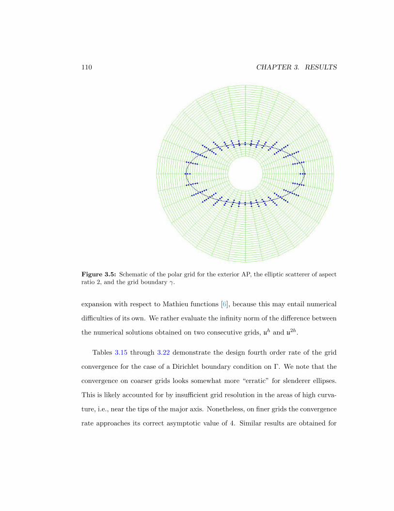
110 CHAPTER 3. RESULTS
Figure 3.5: Schematic of the polar grid for the exterior AP, the elliptic scatterer of aspectratio 2, and the grid boundary γ.
expansion with respect to Mathieu functions [6], because this may entail numerical
difficulties of its own. We rather evaluate the infinity norm of the difference between
the numerical solutions obtained on two consecutive grids, uh and u2h.
Tables 3.15 through 3.22 demonstrate the design fourth order rate of the grid
convergence for the case of a Dirichlet boundary condition on Γ. We note that the
convergence on coarser grids looks somewhat more “erratic” for slenderer ellipses.
This is likely accounted for by insufficient grid resolution in the areas of high curva-
ture, i.e., near the tips of the major axis. Nonetheless, on finer grids the convergence
rate approaches its correct asymptotic value of 4. Similar results are obtained for

3.2. EXTERIOR SCATTERING PROBLEMS 111
Figure 3.6: Schematic of the polar grid for the exterior AP, the elliptic scatterer of aspectratio 10, and the grid boundary γ.
the Neumann boundary condition on Γ, see Tables 3.24 and 3.25, as well as for a
variety of other Dirichlet and Neumann cases that are not presented in these tables.
Grid k0 = 1, M = 12 k0 = 10, M = 37 k0 = 25, M = 69
||uh − u2h||∞ rate ||uh − u2h||∞ rate ||uh − u2h||∞ rate
64× 64 2.737716ee-3 — 6.104800 — 3.945149e+1 —128× 128 3.658040ee-4 2.9038 6.761083e-2 6.4965 1.020563e+2 -1.3712256× 256 2.075372ee-5 4.1396 3.888347e-3 4.1200 3.843873e-1 8.0526512× 512 1.134933ee-6 4.1927 2.382304e-4 4.0287 2.189631e-2 4.13381024× 1024 6.890566ee-8 4.0418 1.481515e-5 4.0072 1.329834e-3 4.04142048× 2048 4.235718ee-9 4.0239 9.247807e-7 4.0018 8.251120e-5 4.01054096× 4096 2.637849ee-10 4.0052 5.778413e-8 4.0004 5.147419e-6 4.0027
Table 3.15: Sound-soft scattering of a plane wave with incidence angle 0 about an ellipsewith aspect ratio 2.

112 CHAPTER 3. RESULTS
Grid k0 = 1, M = 12 k0 = 10, M = 37 k0 = 25, M = 69
||uh − u2h||∞ rate ||uh − u2h||∞ rate ||uh − u2h||∞ rate
64× 64 2.924441e-3 — 1.399531 — 1.588919e+1 —128× 128 3.686772e-4 2.9877 9.024242e-2 3.9550 2.571935e+1 -0.6948256× 256 2.092322e-5 4.1392 5.042251e-3 4.1617 4.528627e-1 5.8276512× 512 1.140182e-6 4.1978 3.077507e-4 4.0342 2.614107e-2 4.11471024× 1024 7.045679e-8 4.0164 1.912254e-5 4.0084 1.576210e-3 4.05182048× 2048 4.352290e-9 4.0169 1.193405e-6 4.0021 9.766250e-5 4.01254096× 4096 2.708936e-10 4.0060 7.456103e-8 4.0005 6.090803e-6 4.0031
Table 3.16: Sound-soft scattering of a plane wave with incidence angle 35 about an ellipsewith aspect ratio 2.
Grid k0 = 1, M = 12 k0 = 10, M = 37 k0 = 25, M = 69
||uh − u2h||∞ rate ||uh − u2h||∞ rate ||uh − u2h||∞ rate
64× 64 3.647013e-2 — 6.942957 — 6.094755e+5 —128× 128 3.229204e-3 3.4975 1.556797e-1 5.4789 8.271102 16.1691256× 256 5.948035e-4 2.4407 5.275428e-3 4.8831 4.000126e-1 4.3700512× 512 2.733103e-5 4.4438 2.869505e-4 4.2004 2.340879e-2 4.09491024× 1024 1.429272e-6 4.2572 1.782570e-5 4.0088 1.410523e-3 4.05272048× 2048 8.252679e-8 4.1143 1.112633e-6 4.0019 8.738691e-5 4.01274096× 4096 5.198425e-9 3.9887 6.951841e-8 4.0004 5.449762e-6 4.0032
Table 3.17: Sound-soft scattering of a plane wave with incidence angle 35 about an ellipsewith aspect ratio 3.
Grid k0 = 1, M = 12 k0 = 10, M = 37 k0 = 25, M = 69
||uh − u2h||∞ rate ||uh − u2h||∞ rate ||uh − u2h||∞ rate
64× 64 2.261699e-2 — 5.730228 — 1.742757e+3 —128× 128 3.149537e-3 2.8442 9.782407e-2 5.8723 9.548658 7.5119256× 256 6.271734e-4 2.3282 4.605138e-3 4.4089 2.276872 2.0682512× 512 2.917059e-5 4.4263 2.738948e-4 4.0716 2.445093e-2 6.54101024× 1024 1.537777e-6 4.2456 1.701433e-5 4.0088 1.483170e-3 4.04312048× 2048 8.870759e-8 4.1156 1.061794e-6 4.0022 9.201076e-5 4.01074096× 4096 5.523241e-9 4.0055 6.633567e-8 4.0006 5.739903e-6 4.0027
Table 3.18: Sound-soft scattering of a plane wave with incidence angle 15 about an ellipsewith aspect ratio 3.
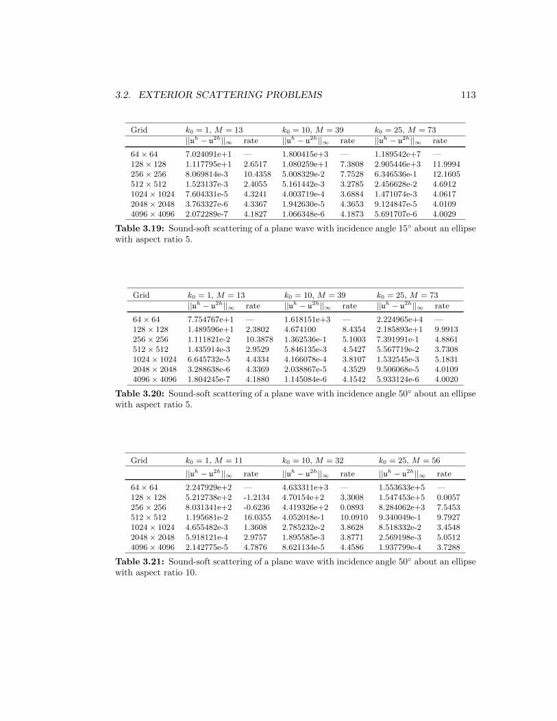
3.2. EXTERIOR SCATTERING PROBLEMS 113
Grid k0 = 1, M = 13 k0 = 10, M = 39 k0 = 25, M = 73
||uh − u2h||∞ rate ||uh − u2h||∞ rate ||uh − u2h||∞ rate
64× 64 7.024091e+1 — 1.800415e+3 — 1.189542e+7 —128× 128 1.117795e+1 2.6517 1.080259e+1 7.3808 2.905446e+3 11.9994256× 256 8.069814e-3 10.4358 5.008329e-2 7.7528 6.346536e-1 12.1605512× 512 1.523137e-3 2.4055 5.161442e-3 3.2785 2.456628e-2 4.69121024× 1024 7.604331e-5 4.3241 4.003719e-4 3.6884 1.471074e-3 4.06172048× 2048 3.763327e-6 4.3367 1.942630e-5 4.3653 9.124847e-5 4.01094096× 4096 2.072289e-7 4.1827 1.066348e-6 4.1873 5.691707e-6 4.0029
Table 3.19: Sound-soft scattering of a plane wave with incidence angle 15 about an ellipsewith aspect ratio 5.
Grid k0 = 1, M = 13 k0 = 10, M = 39 k0 = 25, M = 73
||uh − u2h||∞ rate ||uh − u2h||∞ rate ||uh − u2h||∞ rate
64× 64 7.754767e+1 — 1.618151e+3 — 2.224965e+4 —128× 128 1.489596e+1 2.3802 4.674100 8.4354 2.185893e+1 9.9913256× 256 1.111821e-2 10.3878 1.362536e-1 5.1003 7.391991e-1 4.8861512× 512 1.435914e-3 2.9529 5.846135e-3 4.5427 5.567719e-2 3.73081024× 1024 6.645732e-5 4.4334 4.166078e-4 3.8107 1.532545e-3 5.18312048× 2048 3.288638e-6 4.3369 2.038867e-5 4.3529 9.506068e-5 4.01094096× 4096 1.804245e-7 4.1880 1.145084e-6 4.1542 5.933124e-6 4.0020
Table 3.20: Sound-soft scattering of a plane wave with incidence angle 50 about an ellipsewith aspect ratio 5.
Grid k0 = 1, M = 11 k0 = 10, M = 32 k0 = 25, M = 56
||uh − u2h||∞ rate ||uh − u2h||∞ rate ||uh − u2h||∞ rate
64× 64 2.247929e+2 — 4.633311e+3 — 1.553633e+5 —128× 128 5.212738e+2 -1.2134 4.70154e+2 3.3008 1.547453e+5 0.0057256× 256 8.031341e+2 -0.6236 4.419326e+2 0.0893 8.284062e+3 7.5453512× 512 1.195681e-2 16.0355 4.052018e-1 10.0910 9.340049e-1 9.79271024× 1024 4.655482e-3 1.3608 2.785232e-2 3.8628 8.518332e-2 3.45482048× 2048 5.918121e-4 2.9757 1.895585e-3 3.8771 2.569198e-3 5.05124096× 4096 2.142775e-5 4.7876 8.621134e-5 4.4586 1.937799e-4 3.7288
Table 3.21: Sound-soft scattering of a plane wave with incidence angle 50 about an ellipsewith aspect ratio 10.

114 CHAPTER 3. RESULTS
Grid k0 = 1, M = 13 k0 = 10, M = 39 k0 = 25, M = 73
||uh − u2h||∞ rate ||uh − u2h||∞ rate ||uh − u2h||∞ rate
64× 64 2.448706e+2 — 2.323499 e+4 — 2.151660e+7 —128× 128 4.433401e+2 -0.8564 1.156875e+4 1.0061 3.572665e+6 2.5904256× 256 6.193218e+2 -0.4823 2.889933e+2 5.3231 1.535344e+4 7.8623512× 512 1.050433e-2 15.8474 1.251498e-1 11.1732 4.447023e-1 15.07541024× 1024 5.264725e-3 0.9966 1.706648e-2 2.8744 3.105638e-2 3.83992048× 2048 6.643254e-4 2.9864 1.993312e-3 3.0979 1.968995e-3 3.97944096× 4096 2.408868e-5 4.7855 1.040010e-4 4.2605 2.088858e-4 3.2367
Table 3.22: Sound-soft scattering of a plane wave with incidence angle 50 about an ellipsewith aspect ratio 10.
Grid k0 = 1, M = 13 k0 = 10, M = 35 k0 = 25, M = 61
||uh − u2h||∞ rate ||uh − u2h||∞ rate ||uh − u2h||∞ rate
64× 64 1.181451e-2 — 1.316527 e+1 — 1.879091e+2 —128× 128 3.146854e-4 5.2305 5.405421e-1 4.6062 7.405706e+1 1.3433256× 256 1.566558e-5 4.3282 4.087686e-3 7.0470 3.811382e-1 7.6022512× 512 1.011771e-6 3.9526 2.520713e-4 4.0194 2.007000e-2 4.24721024× 1024 6.381159e-8 3.9869 1.567661e-5 4.0071 1.242483e-3 4.01372048× 2048 4.023256e-9 3.9874 9.784086e-7 4.0020 7.724207e-5 4.00774096× 4096 2.545110e-10 3.9826 6.104984e-8 4.0024 4.834473e-6 3.9980
Table 3.23: Sound-hard scattering of a plane wave with incidence angle 50 about anellipse with aspect ratio 2.
Grid k0 = 1, M = 14 k0 = 10, M = 43 k0 = 25, M = 79
||uh − u2h||∞ rate ||uh − u2h||∞ rate ||uh − u2h||∞ rate
64× 64 5.859690e-2 — 4.558268 — 1.053224e+2 —128× 128 9.846534e-3 2.5731 1.448027e-1 4.9763 4.461393e+1 1.2392256× 256 1.884702e-4 5.7072 8.659281e-3 4.0637 5.844125e-1 6.2544512× 512 9.615561e-6 4.2928 2.363689e-4 5.1951 2.368270e-2 4.62511024× 1024 4.412894e-7 4.4456 1.470104e-5 4.0071 1.454638e-3 4.02512048× 2048 2.845780e-8 3.9548 9.188393e-7 4.0000 9.027833e-5 4.01014096× 4096 1.589844e-9 4.1619 5.934903e-8 3.9525 5.631228e-6 4.0029
Table 3.24: Sound-hard scattering of a plane wave with incidence angle 0 about an ellipsewith aspect ratio 3.

3.2. EXTERIOR SCATTERING PROBLEMS 115
Grid k0 = 1, M = 13 k0 = 10, M = 35 k0 = 25, M = 61
||uh − u2h||∞ rate ||uh − u2h||∞ rate ||uh − u2h||∞ rate
64× 64 3.381436 — 5.287685 — 8.812860e+4 —128× 128 1.076195 1.6517 1.602327 1.7225 6.882858e+1 10.3224256× 256 1.593996e-1 2.7552 5.157602e-1 1.6354 2.620046 4.7153512× 512 1.921666e-3 6.3741 9.974005e-3 5.6924 3.826752e-2 6.09731024× 1024 3.456720e-5 5.7968 2.426475e-4 5.3612 1.628882e-3 4.55422048× 2048 3.522082e-6 3.2949 1.769029e-5 3.7778 1.062220e-4 3.93874096× 4096 1.822888e-7 4.2721 9.543673e-7 4.2123 6.264534e-6 4.0837
Table 3.25: Sound-hard scattering of a plane wave with incidence angle 50 about anellipse with aspect ratio 5.
We also emphasize that the scheme converges with the same design rate for all
angles of incidence, all wavenumbers, and all aspect ratios. The actual values of the
error may, of course, depend on the specific parameters involved. For example, from
Tables 3.16 through 3.25 one can see that as the wavenumber k0 increases while all
other parameters remain the same (the aspect ratio, the grid, etc.), the error also
increases (maximum norm evaluated across the domain). On the other hand, the
angle of incidence does not affect the convergence rate and does not noticeably affect
the actual error either. In Figures 3.7, 3.8 and 3.9 we show the dependence of the
error on the angle of incidence for both sound-soft (Dirichlet boundary condition)
and sound-hard (Neumann boundary condition) scattering about an ellipse of aspect
ratio 3. We see that for both k0 = 3,k0 = 15 and k0 = 30 the error changes by less
than a factor of 2 over the entire 90 range.
For the same setting as before, we also conducted a series of computations that
corroborate the pollution effect. As mentioned in Section 1.2, to maintain the same
level of error for different values of the wavenumber k, the quantity hnkn+1 must
remain constant, where h is the grid size and n is the order of accuracy. This
means, in particular, that if the grid size h is halved, then the same level of error

116 CHAPTER 3. RESULTS
Figure 3.7: Error vs. the angle of incidence for sound-soft (Dirichlet BC) and sound-hard (Neu-mann BC) scattering about an ellipse with aspect ratio 3 for the wavenumber k0 = 3 and thedimension of the basis (2.38) M =21 computed on the polar grid of dimension 1024× 1024.
shall be expected if the wavenumber k increases by a factor of 2n
n+1 . Specifically, the
wavenumber k should increase by a factor of 223 ≈ 1.5874 for the central difference
second order scheme, by a factor of 245 ≈ 1.7411 for the fourth order compact
scheme (1.8), and by a factor of 256 ≈ 1.7818 for the sixth order compact scheme of
[56]. We see that this factor is always less than two, which means that the “points-
per-wavelength” quantity does not stay constant but rather increases as k grows.
However, the higher the accuracy n of the scheme the slower the error increases. In
Table 3.26, we summarize the computational data for all three schemes. Specifically,
we fix the value of k = 4 for the grid of dimension 256× 256, and then vary h and
change k according to the power law 2n
n+1 that corresponds to each scheme.
We next perform complexity profiling of the algorithm. We stress that our
methodology is naturally very effective for problems with several impinging waves

3.2. EXTERIOR SCATTERING PROBLEMS 117
Figure 3.8: Error vs. the angle of incidence for sound-soft (Dirichlet BC) and sound-hard (Neu-mann BC) scattering about an ellipse with aspect ratio 3 for the wavenumber k0 = 15 and thedimension of the basis (2.38) M =52 computed on the polar grid of dimension 1024× 1024.
(a) k0 = 30, M = 86
Figure 3.9: Error vs. the angle of incidence for sound-soft (Dirichlet BC) and sound-hard (Neu-mann BC) scattering about an ellipse with aspect ratio 3 for the wavenumber k0 = 30 and thedimension of the basis (2.38) M =86 computed on the polar grid of dimension 1024× 1024.

118 CHAPTER 3. RESULTS
Grid k M Problem
Diriclet Neumann
||uh − u2h||∞ ||uh − u2h||∞64× 64 1.3195 14 5.088513e-3 1.107942e-3128× 128 2.2974 18 4.707891e-4 1.385318e-4256× 256 4.0000 24 5.628050e-5 1.061957e-5512× 512 6.9644 32 4.670625e-5 4.257857e-51024× 1024 12.125 46 4.203750e-5 3.942691e-52048× 2048 21.112 66 3.922412e-5 3.755659e-54096× 4096 36.758 100 3.764344e-5 3.643574e-5
Table 3.26: Behavior of the schemes for various k — manifestation of the pollution effect.
(see discussion in one dimensional example in Chapter 2 and also Algorithm 11).
This is useful in many practical problems, therefore information about complexity
in solving a scattering problem with multiple incident angles is presented.
Our implementation was written in MATLAB, and the linear systems obtained
from our scheme are solved via MATLAB’s built-in direct sparse solver. The com-
putations were performed on a 2.93 GHz Quad-Core Intel Xeon with 32 Gb of RAM
running on Mac OS X.
In Table 3.27 we present sound-soft scattering of a plane wave about an ellipse
with an aspect ratio of 2 for the wavenumber k0 = 20. The dimension of the basis
(2.38) is M=43. We first solve for an incidence angle of 0 and then use the obtained
information to solve the same problem with an impinging wave at a different incident
angle of 5. Column 4 shows that the computational complexity of the method is
somewhat better than linear as the grid is refined. This behavior is caused by the
direct solver used which was developed in [8]. Column 7 shows the linear behavior
of the computational complexity of the calculation of the second impinging wave.
The matrices Q (2.64) computed for the first impinging wave don’t need to be

3.2. EXTERIOR SCATTERING PROBLEMS 119
recalculated, and therefore the reduced time at this stage is due to the calculation of
the coefficients and obtaining the final solution by solving another auxiliary problem
one more time using the solver from [8], see Section 2.3.6. Column 8 shows the time
saved when a second problem is solved relative to the first one. Similar savings
apply for any number of different incident waves. A sound-hard scattering with the
same setting is presented in Table 3.28. We find a similar linear behavior and a
similar saving of time for the second problem.
Grid 1 wave θ(inc) = 0 2 wave θ(inc) = 5 Saving
||uh − u2h||∞ Time(s) Scaling ||uh − u2h||∞ Time(s) Scaling
64× 64 1.354291e+1 6.2004e-1 — 1.110603e+1 8.7971e-2 — 7.05128× 128 1.234442e-1 1.4990 2.4176 1.317353e-1 1.9846e-1 2.2560 7.55256× 256 6.971178e-3 4.7169 3.1466 7.434611e-3 4.0498e-1 2.0405 11.65512× 512 4.245374e-4 1.7626e+1 3.7368 4.521149e-4 1.1563 2.8553 15.241024× 1024 2.635393e-5 6.6883e+1 3.7944 2.805860e-5 3.9594 3.4240 16.892048× 2048 1.644256e-6 2.6894e+2 4.0211 1.750468e-6 1.6856e+1 4.2571 15.964096× 4096 1.027215e-7 1.4513e+3 5.3963 1.093551e-7 8.7533e+1 5.1929 16.58
Table 3.27: CPU times for sound-soft scattering of a plane wave with incidence angles 0
and 5 about an ellipse with aspect ratio 2 for wavenumber k0 = 20. The dimension of thebasis M=43.
Grid 1 wave θ(inc) = 0 2 wave θ(inc) = 5 Saving
||uh − u2h||∞ Time(s) Scaling ||uh − u2h||∞ Time(s) Scaling
64× 64 6.366639 6.1528e-1 — 5.899738 1.3213e-1 — 4.66128× 128 5.268134 e-1 1.4878 2.4180 1.096330 2.0253e-1 1.5328 7.35256× 256 7.056579e-3 4.7161 3.1700 7.205329e-3 4.0841e-1 2.0166 11.55512× 512 4.305407e-4 1.7395e+1 3.6884 4.414049e-4 1.1562 2.8309 15.051024× 1024 2.680923e-5 6.6856e+1 3.8434 2.748845e-5 3.9751 3.4381 16.822048× 2048 1.673873e-6 2.6953e+2 4.0315 1.715142e-6 1.6876e+1 4.2455 15.974096× 4096 1.046800e-7 1.4521e+3 5.3875 1.071411e-7 8.7569e+1 5.1888 16.58
Table 3.28: CPU times for hard-soft scattering of a plane wave with incidence angles 0
and 5 about an ellipse with aspect ratio 2 for wavenumber k0 = 20. The dimension of thebasis M=43.

120 CHAPTER 3. RESULTS
3.3 Transmission–Reflection problems
3.3.1 Piecewise constant coefficients
The numerical simulation of the simultaneous transmission and scattering of waves
off a given shape (an ellipse) is done using a computational framework similar to that
of Section 3.2, except that instead of setting a boundary condition on Γ we assume
that the medium inside the ellipse is characterized by a constant wavenumber k1
(typically, k1 > k0). At the interface Γ the overall solution and its first normal
derivative are continuous.
The exterior AP and its discretization remain the same as in Section 3.2, while
the interior AP is formulated on the rectangle [−a−0.2, a+ 0.2]× [−b−0.2, b+ 0.2],
where a and b are the major and minor semi-axes of the ellipse, respectively. We
keep a = 1.8 and vary b between 0.9 and 0.15, which yields aspect ratios between 2
and 12. The boundary conditions for the interior AP are zero Dirichlet at the two
horizontal sides of the rectangle, and local Sommerfeld-type conditions (complex) at
its two vertical sides (see (2.34)). The latter guarantees the unique solvability of the
interior AP (no resonances), see [9, Section 4.2] or [42, Section 5.2]. The interior AP
is discretized by the compact scheme [9] with fourth order accuracy on a uniform,
in each coordinate direction, Cartesian grid. It is then solved by a sparse direct
linear solver built into MATLAB. To simplify the monitoring and analysis of the
grid convergence, the grid dimensions for the interior and exterior AP are always
kept the same, i.e., those two grids are refined synchronously. As in Section 3.2, the
convergence is assessed by evaluating the maximum volume norm of the difference
between the numerical solutions obtained on two consecutive grids. In this section

3.3. TRANSMISSION–REFLECTION PROBLEMS 121
though, it is done independently for the exterior and interior parts of the overall
solution.
Grid Exterior
k0 = 1, k1 = 3,M = 18 k0 = 5, k1 = 15,M = 43 k0 = 10, k0 = 30,M = 70
||uh − u2h||∞ rate ||uh − u2h||∞ rate ||uh − u2h||∞ rate
64× 64 4.595301e-3 — 3.193901 — 6.548224e+2 —128× 128 1.680380e-4 4.7733 3.294341e-1 3.2773 1.939342 8.3994256× 256 9.570738e-6 4.1340 1.892338e-3 7.4437 1.929997e-1 3.3289512× 512 4.988526e-7 4.2619 1.133776e-4 4.0610 6.944723e-3 4.79651024× 1024 2.966397e-8 4.0718 6.982484e-6 4.0213 4.325129e-4 4.00512048× 2048 1.713626e-9 4.1136 4.349789e-7 4.0047 2.695934e-5 4.0039
Interior
||uh − u2h||∞ rate ||uh − u2h||∞ rate ||uh − u2h||∞ rate
64× 64 1.580527e-2 — 8.622188 — 7.361263e+2 —128× 128 1.371018e-4 6.8490 4.000175e-1 4.4299 4.175908 7.4617256× 256 8.490845e-6 4.0132 2.746052e-3 7.1866 2.013473e-1 4.3743512× 512 4.202829e-7 4.3365 1.663763e-4 4.0448 8.816271e-3 4.51341024× 1024 2.442490e-8 4.1049 1.028977e-5 4.0152 5.509656e-4 4.00012048× 2048 1.366547e-9 4.1597 6.430838e-7 4.0001 3.435270e-5 4.0035
Table 3.29: Transmission and scattering of a plane wave with incidence angle 40 aboutan ellipse with aspect ratio 2.
The data Tables 3.29, 3.30 and 3.31 demonstrate the grid convergence for two
particular sets of parameters involved. The convergence for other cases that we
have tried with piecewise constant k looks similar. In addition to showing the
convergence data in Tables 3.29, 3.30 and 3.31, we also plot an absolute value and
real and imaginary parts of the solutions that we have computed, see Figures 3.10
through 3.15.

122 CHAPTER 3. RESULTS
Grid Exterior
k0 = 1, k1 = 3,M = 18 k0 = 5, k1 = 15,M = 43 k0 = 10, k0 = 30,M = 70
||uh − u2h||∞ rate ||uh − u2h||∞ rate ||uh − u2h||∞ rate
64× 64 3.397953e-2 — 1.928982 — 1.564833e+4 —128× 128 5.257675e-4 6.0141 1.222531 0.6580 2.540071 12.5889256× 256 2.968034e-5 4.1468 1.256795e-2 6.6040 2.505713 0.0196512× 512 1.621693e-6 4.1939 7.215245e-4 4.1226 5.294069e-2 5.56471024× 1024 8.319173e-8 4.2849 4.686281e-5 3.9445 3.040675e-3 4.12192048× 2048 5.185747e-9 4.0038 2.980399e-6 3.9749 1.824703e-4 4.0587
Interior
||uh − u2h||∞ rate ||uh − u2h||∞ rate ||uh − u2h||∞ rate
64× 64 5.915841e-2 — 4.502945 — 2.997456e+4 —128× 128 4.727249e-4 6.9674 1.476710 1.6085 1.454990e+1 11.0085256× 256 9.910096e-6 5.5760 7.240317e-2 4.3502 3.219025 2.1763512× 512 8.298524e-7 3.5780 7.604703e-4 6.5730 5.533717e-2 5.86221024× 1024 3.405935e-8 4.6067 5.105078e-5 3.8969 3.352915e-3 4.04482048× 2048 2.025545e-9 4.0717 3.330358e-6 3.9382 2.093157e-4 4.0017
Table 3.30: Transmission and scattering of a plane wave with incidence angle 40 aboutan ellipse with aspect ratio 3.
Grid Exterior
k0 = 1, k1 = 3,M = 17 k0 = 5, k1 = 15,M = 42 k0 = 10, k0 = 30,M = 68
||uh − u2h||∞ rate ||uh − u2h||∞ rate ||uh − u2h||∞ rate
128× 128 3.339419 — 1.011317e+2 — 8.966609e+2 —256× 256 2.525248e-3 10.3690 4.429088 4.5131 1.265494e+1 6.1468512× 512 3.016655e-4 3.0654 3.727909e-2 6.8925 5.603543e-1 4.49721024× 1024 7.296313e-5 2.0477 4.070004e-3 3.1953 6.315946e-3 6.47122048× 2048 9.046537e-6 3.0117 3.237602e-4 3.6520 3.668013e-4 4.1059
Interior
||uh − u2h||∞ rate ||uh − u2h||∞ rate ||uh − u2h||∞ rate
128× 128 2.895946 — 7.446942e+2 — 4.085428e+4 —256× 256 2.649119e-3 10.0943 4.907694 7.2455 1.662587e+2 7.9409512× 512 2.590272e-4 3.3543 4.386424e-2 6.8059 1.008079 7.36571024× 1024 5.793892e-5 2.1605 3.933254e-3 3.4792 8.501939e-3 6.88962048× 2048 6.983459e-6 3.0525 3.009321e-4 3.7082 3.740583e-4 4.5065
Table 3.31: Transmission and scattering of a plane wave with incidence angle 40 aboutan ellipse with aspect ratio 12.

3.3. TRANSMISSION–REFLECTION PROBLEMS 123
(a) Aspect ratio 2
(b) Aspect ratio 10
Figure 3.10: Transmission and scattering of a plane wave with incidence angle 40 aboutan ellipse with k1 = 20 (inside) and k0 = 10 (outside). Absolute value of the total field isshown. The grid dimension is 1024× 1024 for both the interior AP (Cartesian) and exteriorAP (polar).

124 CHAPTER 3. RESULTS
(a) Aspect ratio 2
(b) Aspect ratio 10
Figure 3.11: Transmission and scattering of a plane wave with incidence angle 40 aboutan ellipse with k1 = 20 (inside) and k0 = 10 (outside). Absolute value of the total field isshown. The grid dimension is 1024× 1024 for both the interior AP (Cartesian) and exteriorAP (polar).

3.3. TRANSMISSION–REFLECTION PROBLEMS 125
(a) Aspect ratio 2
(b) Aspect ratio 10
Figure 3.12: Transmission and scattering of a plane wave with incidence angle 40 aboutan ellipse with k1 = 20 (inside) and k0 = 10 (outside). Absolute value of the total field isshown. The grid dimension is 1024× 1024 for both the interior AP (Cartesian) and exteriorAP (polar).

126 CHAPTER 3. RESULTS
(a) Aspect ratio 3
(b) Aspect ratio 5
Figure 3.13: Transmission and scattering of a plane wave with incidence angle 180 aboutan ellipse with k1 = 20 (inside) and k0 = 10 (outside). Absolute value of the total field isshown. The grid dimension is 513 × 513 for both the interior AP (Cartesian) and exteriorAP (polar).

3.3. TRANSMISSION–REFLECTION PROBLEMS 127
(a) Aspect ratio 3
(b) Aspect ratio 5
Figure 3.14: Transmission and scattering of a plane wave with incidence angle 180 aboutan ellipse with k1 = 20 (inside) and k0 = 10 (outside). Absolute value of the total field isshown. The grid dimension is 513 × 513 for both the interior AP (Cartesian) and exteriorAP (polar).
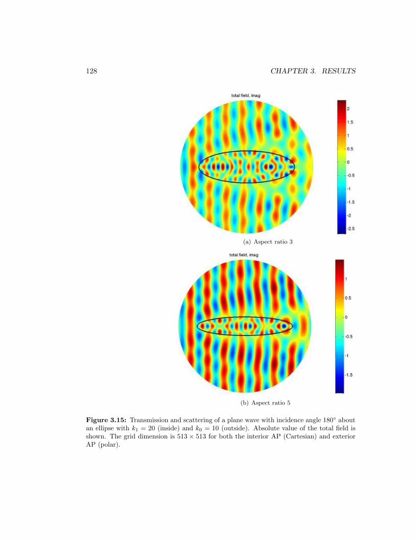
128 CHAPTER 3. RESULTS
(a) Aspect ratio 3
(b) Aspect ratio 5
Figure 3.15: Transmission and scattering of a plane wave with incidence angle 180 aboutan ellipse with k1 = 20 (inside) and k0 = 10 (outside). Absolute value of the total field isshown. The grid dimension is 513 × 513 for both the interior AP (Cartesian) and exteriorAP (polar).

3.3. TRANSMISSION–REFLECTION PROBLEMS 129
3.3.2 Piecewise smooth coefficients
In this section, we keep the computational setting the same as in Section 3.3.1,
except that we allow for a smooth variation of the wavenumber inside the ellipse:
k =
k1e−10(r−r0)6r6 , if r 6 r0,
k1, if r > r0,
(3.8)
where r =√x2 + y2 and r0 = 1.6. The variable coefficient Helmholtz equation
is approximated with fourth order accuracy by the compact scheme of [9]. In Ta-
ble 3.32, we show the results for the ellipse with aspect ratio 2: a = 1.8 and b = 0.9.
In Table 3.33, we show the results for the ellipse with aspect ratio 3: a = 1.8 and
b = 0.6. In Table 3.34, we show the results for the ellipse with aspect ratio 5: a = 1.8
and b = 0.36. These results corroborate the design fourth order convergence rate of
the algorithm in the case of variable coefficients.
Grid Exterior
k0 = 1, k1 = 3,M = 50 k0 = 5, k1 = 15,M = 50 k0 = 10, k0 = 30,M = 69
||uh − u2h||∞ rate ||uh − u2h||∞ rate ||uh − u2h||∞ rate
128× 128 1.196903e-1 — 2.740357 — 9.679627 —256× 256 8.888395e-4 7.0732 1.071586e-1 4.6765 8.093132e-1 3.5802512× 512 5.054118e-5 4.1364 1.339804e-3 6.3216 8.933817e-3 6.50131024× 1024 9.918967e-7 5.6711 4.031620e-5 5.0545 5.392737e-4 4.05022048× 2048 7.239554e-8 3.7762 2.729896e-6 3.8844 4.167435e-5 3.6938
Interior
||uh − u2h||∞ rate ||uh − u2h||∞ rate ||uh − u2h||∞ rate
128× 128 2.169952e-1 — 5.413927 — 2.473694e+1 —256× 256 1.267208e-3 7.4199 1.422706e-1 5.2500 1.466237 4.0765512× 512 4.573756e-5 4.7921 1.506757e-3 6.5610 5.642709e-2 4.69961024× 1024 6.765407e-7 6.0791 2.968551e-5 5.6655 4.756129e-4 6.89052048× 2048 5.114153e-8 3.7256 2.285437e-6 3.6992 2.445819e-5 4.2814
Table 3.32: Transmission and scattering of a plane wave with incidence angle 40 about aninhomogeneous ellipse with aspect ratio 2 and interior wavenumber given by formula ( 3.8).

130 CHAPTER 3. RESULTS
Grid Exterior
k0 = 1, k1 = 3,M = 44 k0 = 5, k1 = 15,M = 43 k0 = 10, k0 = 30,M = 70
||uh − u2h||∞ rate ||uh − u2h||∞ rate ||uh − u2h||∞ rate
128× 128 1.342633e-3 — 3.189426e-1 — 2.273503 —256× 256 4.704559e-5 4.8349 2.112324e-3 7.2383 1.428778 0.6701512× 512 1.972406e-6 4.5760 1.037815e-4 4.3472 8.515279e-3 7.39051024× 1024 1.128138e-7 4.1279 6.701632e-6 3.9529 4.664540e-4 4.19022048× 2048 6.620319e-9 4.0909 5.703865e-7 3.5545 2.867676e-5 4.0238
Interior
||uh − u2h||∞ rate ||uh − u2h||∞ rate ||uh − u2h||∞ rate
128× 128 3.067343e-3 — 1.043931 — 9.253122 —256× 256 6.693782e-5 5.5180 3.225823e-2 5.0162 2.960923 1.6439512× 512 1.396376e-6 5.5831 1.002967e-4 8.3292 4.859728e-2 5.92901024× 1024 8.178574e-8 4.0937 6.580268e-6 3.9300 4.749737e-4 6.67692048× 2048 5.333208e-9 3.9388 4.146442e-7 3.9882 2.935093e-5 4.0164
Table 3.33: Transmission and scattering of a plane wave with incidence angle 40 about aninhomogeneous ellipse with aspect ratio 3 and interior wavenumber given by formula ( 3.8).
Grid Exterior
k0 = 1, k1 = 3,M = 50 k0 = 5, k1 = 15,M = 50 k0 = 10, k0 = 30,M = 69
||uh − u2h||∞ rate ||uh − u2h||∞ rate ||uh − u2h||∞ rate
128× 128 1.196903e-1 — 2.740357 — 9.679627 —256× 256 8.888395e-4 7.0732 1.071586e-1 4.6765 8.093132e-1 3.5802512× 512 5.054118e-5 4.1364 1.339804e-3 6.3216 8.933817e-3 6.50131024× 1024 9.918967e-7 5.6711 4.031620e-5 5.0545 5.392737e-4 4.05022048× 2048 7.239554e-8 3.7762 2.729896e-6 3.8844 4.167435e-5 3.6938
Interior
||uh − u2h||∞ rate ||uh − u2h||∞ rate ||uh − u2h||∞ rate
128× 128 2.169952e-1 — 5.413927 — 2.473694e+1 —256× 256 1.267208e-3 7.4199 1.422706e-1 5.2500 1.466237 4.0765512× 512 4.573756e-5 4.7921 1.506757e-3 6.5610 5.642709e-2 4.69961024× 1024 6.765407e-7 6.0791 2.968551e-5 5.6655 4.756129e-4 6.89052048× 2048 5.114153e-8 3.7256 2.285437e-6 3.6992 2.445819e-5 4.2814
Table 3.34: Transmission and scattering of a plane wave with incidence angle 40 about aninhomogeneous ellipse with aspect ratio 5 and interior wavenumber given by formula ( 3.8).

Chapter 4
Discussion and Conclusion
4.1 Discussion
We have described a combined implementation of the method of difference poten-
tials along with the compact high order accurate finite difference schemes for the
numerical solution of wave propagation problems in the frequency domain. The
governing Helmholtz equation is approximated on a regular structured grid, which
is efficient and entails a low computational complexity. At the same time, the
method guarantees no loss of accuracy for curvilinear non-conforming boundaries,
and can also handle variable coefficients that describe a non-homogeneous medium.
As such, the resulting method provides a viable alternative to both BEM and high
order FEM.
The performance of the method and, in particular, its design high order accu-
racy, has been corroborated numerically by solving a variety of 2D interior, exterior,
131

132 CHAPTER 4. DISCUSSION AND CONCLUSION
and reflection/transmission Helmholtz problems, including those with variable co-
efficients, on Cartesian and Polar grids for non-conforming boundaries/interfaces
shaped as circles and ellipses.
Among other advantages of the proposed methodology is its capability to accu-
rately reconstruct the solution and/or its normal derivative directly at the boundary.
This is done without interpolating and/or using one-sided differences, such as in con-
ventional FD, and with no additional developments needed as in FEM, see, e.g., [11].
Additional advantages of the method are the absence of any singular integrals or
similar constructs, the minimum number of unknowns that characterize the discrete
solution — just one per grid node, and the same number of boundary conditions
needed for the scheme as that needed for the underlying differential equation.
For exterior problems we constructed auxiliary problems (see Section 2.3.2.2)
with the appropriate artificial boundary conditions (ABCs), see [64]. For the con-
stant coefficient 2D Helmholtz equation (typical for the far field), the APs were
formulated using polar coordinates, which enables a natural and efficient implemen-
tation of the exact non-local ABCs in Fourier space. The proposed methodology is
extended for the combined reflection/transmission problems. The latter formulation
involves a joint solution of the interior and exterior Calderon’s BEPs constructed at
the interface between the interior and exterior sub-regions.
Thus far, we have computed solutions only for circular and elliptical boundaries.
The case of general smooth boundaries was analyzed theoretically in [42, Appendix
A], and the corresponding Taylor-based extension operators have been developed.

4.2. CONCLUSIONS AND FUTURE RESEARCH 133
4.2 Conclusions and future research
We have simulated a broad range of constant and variable coefficient 2D test cases
for non-conforming boundaries/interfaces on regular structured grids. Our com-
putations convincingly corroborate the design high order accuracy of the proposed
method.
A study is needed to explore alternative strategies for choosing M – the dimen-
sion of the basis used for representing the solution at the boundary Γ as in (2.38) or
(2.59). In addition to that, the possibility of using other bases has to be examined.
The ideas of reduced order modeling [26] (or, similarly, principal component analysis
or proper orthogonal decomposition) has to be investigated to further reduce the
dimension of the basis on Γ. Other bases may be more convenient to use like in the
case of piece-wise parametrization [10].
Actual computations of the scattering and transmission/scattering solutions for
arbitrarily shaped domains (other than circles or ellipses) will need to be performed.
The corresponding general construct of the equation based extension has been de-
veloped in [42, Appendix A].
The domains of a more general shape (beyond circles and ellipses) have to be
developed. Arbitrary smooth boundaries will require a more general construction
of the extension operators (see Appendix in [42]).
Yet another direction for future work will be to allow for multiple sub-regions,
for example, multiple scatterers immersed into the same background medium. The
simplest case will amount to considering a piece-wise constant function k2(x, y) in

134 CHAPTER 4. DISCUSSION AND CONCLUSION
the Helmholtz equation (1.1), while more elaborate settings may also include the
variation of material characteristics.
The proposed methodology needs to be extended to 3D wave propagation which
requires that the coordinates associated with a curve be replaced with surface-
oriented coordinates, see [32].
Finally, the extension of the proposed methodology to time-dependent prob-
lems (e.g., the wave, i.e., d’Alembert, equation instead of the Helmholtz equation)
requires additional theoretical developments.
Note, that even though the current implementation and discussion focuses on
wave propagation problems, the method of difference potentials is capable of ad-
dressing a considerably broader range of formulations, including problems in heat
transfer, elasticity, fluid dynamics, and other areas, see for example [52].

Bibliography
[1] S. Abarbanel and A. Ditkowski. Asymptotically stable fourth-order accurate
schemes for the diffusion equation on complex shapes. J. Comput. Phys.,
133(2):279–288, 1997.
[2] I. M. Babuska and S.A. Sauter. Is the pollution effect of the FEM avoidable
for the Helmholtz equation considering high wave numbers? SIAM Journal on
Numerical Analysis, 34(6):2392–2423, 1997.
[3] G. Baruch, G. Fibich, and S. Tsynkov. High-order numerical method for the
nonlinear Helmholtz equation with material discontinuities in one space dimen-
sion. J. Comput. Phys., 227:820–850, 2007.
[4] G. Baruch, G. Fibich, S. Tsynkov, and E. Turkel. Fourth order scheme for
wave-like equations in frequency space with discontinuities in the coefficients.
Communications in Computational Physics, 5(2–4):442–455, 2009.
[5] A. Bayliss, C. I. Goldstein, and E. Turkel. On accuracy conditions for the
numerical computation of waves. J. Comput. Phys., 59(3):396–404, 1985.
[6] J. J. Bowman, T. B. A. Senior, and P. L. E. Uslenghi, editors. Electromag-
135

136 BIBLIOGRAPHY
netic and Acoustic Scattering by Simple Shapes. A Summa Book. Hemisphere
Publishing Corp., New York, 1987. Revised reprint of the 1969 edition.
[7] S. C. Brenner and L. Ridgway Scott. The Mathematical Theory of Finite El-
ement Methods, volume 15 of Texts in Applied Mathematics. Springer-Verlag,
New York, second edition, 2002.
[8] S. Britt, S. Tsynkov, and E. Turkel. A compact fourth order scheme for the
Helmholtz equation in polar coordinates. J. Sci. Comput., 45(1-3):26–47, 2010.
[9] S. Britt, S. Tsynkov, and E. Turkel. Numerical simulation of time-harmonic
waves in inhomogeneous media using compact high order schemes. Commun.
Comput. Phys., 9(3):520–541, March 2011.
[10] S. Britt, S. Tsynkov, and E. Turkel. A high order numerical method for the
Helmholtz equation with non-standard boundary conditions. SIAM Journal on
Scientific Computing, 2012. [Submitted for publication].
[11] G. F. Carey, S.-S. Chow, and M. K. Seager. Approximate boundary-flux cal-
culations. Comput. Methods Appl. Mech. Engrg., 50(2):107–120, 1985.
[12] H. Cheng, L. Greengard, and V. Rokhlin. A fast adaptive multipole algorithm
in three dimensions. J. Comput. Phys., 155(2):468–498, 1999.
[13] P. G. Ciarlet. The Finite Element Method for Elliptic Problems, volume 40 of
Classics in Applied Mathematics. Society for Industrial and Applied Mathe-
matics (SIAM), Philadelphia, PA, 2002. Reprint of the 1978 original [North-
Holland, Amsterdam; MR0520174 (58 #25001)].

BIBLIOGRAPHY 137
[14] L. Collatz. The Numerical Treatment of Differential Equations. New York:
Springer, 1966.
[15] S. Conte and C. de Boor. Elementary Numerical Analysis: An Algorithmic
Approach. McGraw-Hill, New York, third edition, 1980.
[16] R. K. Crockett, P. Colella, and D. T. Graves. A Cartesian grid embedded
boundary method for solving the Poisson and heat equations with discontinuous
coefficients in three dimensions. J. Comput. Phys., 230(7):2451–2469, 2011.
[17] A. Ditkowski and M. Sever. On the intersection of sets of incoming and outgoing
waves. Quart. Appl. Math., 66(1):1–26, 2008.
[18] Y. A. Erlangga. Advances in iterative methods and preconditioners for the
Helmholtz equation. Arch. Comput. Methods Eng., 15(1):37–66, 2008.
[19] Y. A. Erlangga, C. W. Oosterlee, and C. Vuik. A novel multigrid based pre-
conditioner for heterogeneous Helmholtz problems. SIAM J. Sci. Comput.,
27(4):1471–1492 (electronic), 2006.
[20] Y. A. Erlangga and E. Turkel. Iterative schemes for high order compact dis-
cretizations to the exterior Helmholtz equation. Mathematical Modeling and
Numerical Analysis (ESAIM: M2AN), 2011. [To appear].
[21] Y. A. Erlangga, C. Vuik, and C. W. Oosterlee. On a class of preconditioners for
solving the Helmholtz equation. Appl. Numer. Math., 50(3-4):409–425, 2004.
[22] C. Farhat, I. Harari, and L.P. Franca. The discontinuous enrichment method.
Computer Meth. in Appl. Mech. & Eng., 190:6455–6479, 2001.
138 BIBLIOGRAPHY
[23] C. Farhat, R. Tezaur, and J. Toivanen. A domain decomposition method for
discontinuous Galerkin discretizations of Helmholtz problems with plane waves
and Lagrange multipliers. International Journal for Numerical Methods in En-
gineering, 78:1513–1531, 2009.
[24] W. Fong and E. Darve. The black-box fast multipole method. J. Comput.
Phys., 228(23):8712–8725, 2009.
[25] L. Greengard and V. Rokhlin. A fast algorithm for particle simulations. J.
Comput. Phys., 73(2):325–348, 1987.
[26] M. Gunzburger and J. Peterson. Reduced-order modeling of complex systems
with multiple system parameters. In Large-scale scientific computing, volume
3743 of Lecture Notes in Comput. Sci., pages 15–27. Springer, Berlin, 2006.
[27] B. Gustafsson. The convergence rate for difference approximations to general
mixed initial-boundary value problems. SIAM Journal on Numerical Analysis,
18(2):179–190, 1981.
[28] Bertil Gustafsson. The convergence rate for difference approximations to mixed
initial boundary value problems. Mathematics of Computation, 29(130):396–
406, 1975.
[29] T. Hagstrom. Radiation boundary conditions for the numerical simulation of
waves. In A. Iserlis, editor, Acta Numerica, volume 8, pages 47–106, Cambridge,
1999. Cambridge University Press.
[30] William D. Henshaw. A high-order accurate parallel solver for Maxwell’s equa-

BIBLIOGRAPHY 139
tions on overlapping grids. SIAM J. Sci. Comput., 28(5):1730–1765 (electronic),
2006.
[31] J. S. Hesthaven and T. Warburton. Nodal discontinuous Galerkin methods,
volume 54 of Texts in Applied Mathematics. Springer, New York, 2008. Algo-
rithms, analysis, and applications.
[32] E. H. Hirschel and W. Kordulla. Shear Flow in Surface-Oriented Coordinates,
volume 4 of Notes on Numerical Fluid Mechanics. Friedr. Vieweg & Sohn
Verlagsgesellschaft mbH, Braunschweig/Wiesbaden, 1981-1986.
[33] R. Hixon and E. Turkel. Compact implicit MacCormack-type schemes with
high accuracy. J. Comput. Phys., 158(1):51–70, 2000.
[34] R. Holland. Pitfalls of staircase meshing. IEEE Trans. Electromagnetic Com-
patibility, 35:434–439, 1993.
[35] F. Ihlenburg. Finite Element Analysis of Acoustic Scattering, volume 132 of
Applied Mathematical Sciences. Springer, 1998.
[36] H. Johansen and P. Colella. A Cartesian grid embedded boundary method for
Poisson’s equation on irregular domains. J. Comput. Phys., 147(1):60–85, 1998.
[37] R. J. LeVeque and Z. Li. The immersed interface method for elliptic equations
with discontinuous coefficients and singular sources. SIAM J. Numer. Anal.,
31(4):1019–1044, 1994.
[38] Z. Li and K. Ito. The Immersed Interface Method, volume 33 of Frontiers in
Applied Mathematics. Society for Industrial and Applied Mathematics (SIAM),

140 BIBLIOGRAPHY
Philadelphia, PA, 2006. Numerical solutions of PDEs involving interfaces and
irregular domains.
[39] J. Loncaric, V. S. Ryaben’kii, and S. V. Tsynkov. Active shielding and control
of noise. SIAM J. Applied Math., 62(2):563–596, 2001.
[40] P. G. Martinsson. Fast multiscale methods for lattice equations. PhD thesis,
Texas Institute for Computational and Applied Mathematics, The University
of Texas at Austin, Austin, TX, USA, 2002.
[41] M. Medvinsky. Comparison of local absorbing radiation conditions for scatter-
ing about elliptical body. Master’s thesis, Tel Aviv University, 2007.
[42] M. Medvinsky, S. Tsynkov, and E. Turkel. The method of difference potentials
for the Helmholtz equation using compact high order schemes. J. Sci. Comput.,
53(1):150–193, 2012.
[43] M. Medvinsky and E. Turkel. On surface radiation conditions for an ellipse.
Journal of Computational and Applied Mathematics, 234(6):1647–1655, 2010.
[44] M. Medvinsky, E. Turkel, and U. Hetmaniuk. Local absorbing boundary con-
ditions for elliptical shaped bodies. J. Comput. Phys., 227:8254–8267, 2008.
[45] C. S. Peskin. The immersed boundary method. Acta Numer., 11:479–517, 2002.
[46] D. Pissoort, E. Michielssen, and A. Grbic. An electromagnetic crystal Green
function multiple scattering technique for arbitrary polarizations, lattices, and
defects. J. of Lightwave Technology, 25(2):571–583, 2007.
[47] A. A. Reznik. Approximation of surface potentials of elliptic operators by
difference potentials. Dokl. Akad. Nauk SSSR, 263(6):1318–1321, 1982.

BIBLIOGRAPHY 141
[48] A. A. Reznik. Approximation of the surface potentials of elliptic operators
by difference potentials and solution of boundary-value problems. PhD thesis,
Moscow Institute for Physics and Technology, Moscow, USSR, 1983. [in Rus-
sian].
[49] R. D. Richtmyer. Difference methods for initial-value problems. Interscience
tracts in pure and applied mathematics. Tract 4. Interscience Publishers, Inc.,
New. York, 1957.
[50] V. S. Ryaben’kii. Boundary equations with projections. Russian Math. Surveys,
40(2):147–183, 1985.
[51] V. S. Ryaben’kii. Boundary equations with projections. Russian Math. Surveys,
40(2):147–183, 1985.
[52] V. S. Ryaben’kii. Method of Difference Potentials and Its Applications, vol-
ume 30 of Springer Series in Computational Mathematics. Springer-Verlag,
Berlin, 2002.
[53] V. S. Ryaben’kii. Method of Difference Potentials and Its Applications, vol-
ume 30 of Springer Series in Computational Mathematics. Springer-Verlag,
Berlin, 2002.
[54] V. S. Ryaben’kii and A. F. Filippov. On Stability of Difference Equations.
Gosudarstv. Izdat. Tehn.-Teor. Lit., Moscow, 1956. [Russian].
[55] I. Singer and E. Turkel. High-order finite difference methods for the Helmholtz
equation. Comput. Methods Appl. Mech. Engrg., 163(1-4):343–358, 1998.

142 BIBLIOGRAPHY
[56] I. Singer and E. Turkel. Sixth-order accurate finite difference schemes for the
Helmholtz equation. J. Comput. Acoust., 14(3):339–351, 2006.
[57] I. A. Stegun and M. Abramowitz. Handbook of Mathematical Functions: With
Formulas, Graphs, and Mathematical Tables. National Bureau of Standards,
1968.
[58] G. Strang and G. J. Fix. An Analysis of the Finite Element Method. Prentice
Hall, Englewood Cliffs, NJ, 1973.
[59] M. Svard and J. Nordstrom. On the order of accuracy for difference approxi-
mations of initial-boundary value problems. Journal of Computational Physics,
218(1):333–352, 2006.
[60] K. Taira and T. Colonius. The immersed boundary method: a projection
approach. Journal of Computational Physics, 225(2):2118–2137, 2007.
[61] H. Tal-Ezer and E. Turkel. The iterative solver Risolv with application to the
exterior Helmholtz problem. SIAM J. Sci. Comput., 32(1):463–475, 2010.
[62] Y.H. Tseng and J.H. Ferziger. A ghost-cell immersed boundary method for
flow in complex geometry. Journal of Computational Physics, 192(2):593–623,
2003.
[63] I. Tsukerman. A class of difference schemes with flexible local approximation.
J. Comput. Phys., 211(2):659–699, 2006.
[64] S. V. Tsynkov. Numerical solution of problems on unbounded domains. A
review. Appl. Numer. Math., 27(4):465–532, 1998.

BIBLIOGRAPHY 143
[65] E. Turkel, D. Gordon, R. Gordon, and S. Tsynkov. Compact 2d and 3d sixth
order schemes for the helmholtz equation with variable wave number. Journal
of Computational Physics, 2012.
[66] E. Turkel and A. Yefet. On the construction of a high order difference scheme
for complex domains in a Cartesian grid. Appl. Numer. Math., 33(1-4):113–124,
2000.
[67] J. C. G. Vega and S. C. Cerda. Theory and numerical analysis of the Mathieu
functions. Tecnologico de Monterrey, Mexico report and the references given in
this paper, 2003.
[68] S. Xu. A boundary condition capturing immersed interface method for 3D rigid
objects in a flow. J. Comput. Phys., 230(19):7176–7190, 2011.
[69] A. Yefet and E. Turkel. Fourth order compact implicit method for the Maxwell
equations with discontinuous coefficients. Appl. Numer. Math., 33(1-4):125–
134, 2000.
[70] L. Ying, G. Biros, and D. Zorin. A kernel-independent adaptive fast multipole
algorithm in two and three dimensions. J. Comput. Phys., 196(2):591–626,
2004.
[71] C. Zhang and R. J. LeVeque. The immersed interface method for acoustic wave
equations with discontinuous coefficients. Wave Motion, 25(3):237–263, 1997.
[72] X. Zhong. A new high-order immersed interface method for solving elliptic equa-
tions with imbedded interface of discontinuity. J. Comput. Phys., 225(1):1066–
1099, 2007.

144 BIBLIOGRAPHY
[73] Y. C. Zhou and G. W. Wei. On the fictitious-domain and interpolation for-
mulations of the matched interface and boundary (MIB) method. J. Comput.
Phys., 219(1):228–246, 2006.
[74] Y. C. Zhou, S. Zhao, M. Feig, and G. W. Wei. High order matched interface
and boundary method for elliptic equations with discontinuous coefficients and
singular sources. J. Comput. Phys., 213(1):1–30, 2006.


תקציר
המופרד קבוע, בהכרח לא אך חלק, טווח של גדולים אזורים פני על גלים התפשטות חוקרים אנו
ומשול הפרד בשיטת משתמשים אנו שרירותית. צורה בעלי ממשקים ידי על תחומים לתת
פתרונות של מסט מורכב לבעיה הפתרון ויוצאים. נכנסים לגלים הגל חלוקת על המבוססת
בעיית של הבחירה תחום. תת לכל תלוי בלתי באופן מוגדרת עזר בעיית עזר. לבעיית פרטיים
החדשה השיטה וחסכוני. קל נומרי פתרון המאפשרת בצורה לנסחה ניתן יחסית: גמישה היא עזר
קשר ללא ופולריות, קרטזיות רשתות כגון ומובנות, פשוטות נומריות ברשתות רק משתמשת שלנו
משתמשת היא חלקים, באזורים הממשקים. צורת או הבעיה של התחום גבולות של לצורתם
נוספים שפה תנאיי דורשים אינם אשר גבוהה דיוק מסדר קומפקטית סופיים הפרשים בסכמת
הרשת על יושבים אינם אשר ממשקים עצמה. הדיפרנציאלית למשוואה הנדרשים אלו מלבד
.[74] ההפרשיים הפוטנציאלים ושיטת קלדרון של אופרטור ידי על מטופלים הנומרית
מטפל הוא חשובים: יתרונות מספר ההפרשיים הפוטנציאלים ולשיטת קלדרון של לאופרטור
היא המורכבות ואילו כלליים שפה ותנאי משתנים מקדמים עקומים, וממשקים בגבולות בקלות
שהמתודולוגיה הוא העיקרי היתרון רגילה. מובנית רשת על הסופיים, ההפרשים סכימת של זה
יותר. מסורתיות בגישות הכרוכים הקשיים על ומתגברת גבוה וסדר דיוק מספקת הזו


לילדיי
על טורקל אלי לפרופסור העמוקה והערכתי תודתי את להביע ברצוני
ובמהלך זה מחקר במהלך הרבה והתמיכה המתמדת המעורבות הסבלנות,
פעולה. ושיתוף היכרות שנות שבע
ייעוץ הדרכה, על צנקוב סמיון לפרופסור תודה אסיר אני כן, כמו
קרוליינה. צפון באוניברסיטת נשכחת בלתי התמחות עבור במיוחד וידידות,
נעשת. הייתה לא לעולם זו עבודה שלו והעידוד העזרה ללא
התומכים, להוריי והאהבה. הסבלנות על למשפחתי מודה אני כמובן,
יכול לא לעולם זה מחקר בלעדיהם המקסימים. והילדים המתחשבת אישתי
כמשמעו). (פשוטו להתקיים היה
בשבילי "שם" שהיו והחברים המשפחה בני לכל תודתי את להביע ברצוני
לעיל. מופיע לא שמם אך זו, ארוכה בתקופה


המנחים בהדרכת נעשתה זו עבודה
תל־אביב אוניברסיטת טורקל, אלי פרופסור
קרוליינה צפון אוניברסיטת צנקוב, סמיון ופרופסור


תל־אביב אוניברסיטתסאקלר ובברלי ריימונד שם על מדויקים למדעים הפקולטה
המתמטיקה למדעי ביה"ס
שימושית למתמטיקה החוג
גלים עבור גבוה מסדר נומריות שיטות
חורגים וממשקים רגילות ברשתות שימוש תוך
לפילוסופיה" "דוקטור תואר קבלת לשם חבור
ידי על
מיכאל מדבינסקי
תל־אביב אוניברסיטת של לסנט הוגש
2013 באוקטובר 6