high-frequency homogenization for periodic...

Proc. R. Soc. A (2010) 466, 2341–2362doi:10.1098/rspa.2009.0612

Published online 10 March 2010

High-frequency homogenizationfor periodic media

BY R. V. CRASTER1,*, J. KAPLUNOV2 AND A. V. PICHUGIN2

1Department of Mathematical and Statistical Sciences, University of Alberta,Edmonton, Canada T6G 2G1

2Department of Mathematical Sciences, Brunel University, Uxbridge,Middlesex UB8 3PH, UK

An asymptotic procedure based upon a two-scale approach is developed for wavepropagation in a doubly periodic inhomogeneous medium with a characteristic lengthscale of microstructure far less than that of the macrostructure. In periodic media, thereare frequencies for which standing waves, periodic with the period or double period ofthe cell, on the microscale emerge. These frequencies do not belong to the low-frequencyrange of validity covered by the classical homogenization theory, which motivates ouruse of the term ‘high-frequency homogenization’ when perturbing about these standingwaves. The resulting long-wave equations are deduced only explicitly dependent uponthe macroscale, with the microscale represented by integral quantities. These equationsaccurately reproduce the behaviour of the Bloch mode spectrum near the edges of theBrillouin zone, hence yielding an explicit way for homogenizing periodic media in thevicinity of ‘cell resonances’. The similarity of such model equations to high-frequencylong wavelength asymptotics, for homogeneous acoustic and elastic waveguides, validin the vicinities of thickness resonances is emphasized. Several illustrative examples areconsidered and show the efficacy of the developed techniques.

Keywords: Floquet–Bloch waves; stop bands; photonics;high-frequency long waves; homogenization

1. Introduction

Many structures are constructed from composites with periodic, or doublyperiodic, variations in material parameters. The varied, and sometimesunexpected, wave propagation properties of composites (Milton 2002) havemotivated a number of remarkable new applications, including, but not limitedto, photonic crystals and microstructured fibres (Joannopoulos et al. 1995; Zollaet al. 2005), as well as the rapidly developing area of metamaterials (Smithet al. 2004). Thus, there is considerable interest in modelling wave propagationthrough media with regularly spaced defects or inhomogeneities. Direct numericalsimulation using finite elements (Zolla et al. 2005) is popular, but can become

*Author for correspondence ([email protected]).

Received 17 November 2009Accepted 4 February 2010 This journal is © 2010 The Royal Society2341

on May 12, 2018http://rspa.royalsocietypublishing.org/Downloaded from

mailto:[email protected]

http://rspa.royalsocietypublishing.org/

2342 R. V. Craster et al.

intensive for large-scale media with many small inclusions even if calculated overa single cell with Floquet–Bloch conditions invoked. In the latter case, progresscan also be made using Rayleigh’s multipole method (Rayleigh 1892) and modernextensions and refinements are possible (Movchan et al. 2002; Poulton et al.in press). Another popular procedure is the plane wave expansion method thatamounts to expanding all relevant fields over the cell into Fourier series andsolving the resulting infinite system of linear equations (Kushwaha et al. 1993;Andrianov et al. 2008).

Complementary to this literature is that of homogenization, which involvestaking a medium with rapidly oscillatory material properties on a fine microscaleand averaging these out, in some fashion, to obtain an equivalent homogeneousmaterial with effective material parameters. This is naturally convenient asit buries the microstructure into coefficients, and computations (or analysis)are then just performed on the macroscale. The development of traditionaltechniques of asymptotic homogenization has been strongly focused on recoveringthe classical limiting behaviours in effective media (Sanchez-Palencia 1980;Bakhvalov & Panasenko 1989). This usually implies slow variation of relevantfields both on the microscale and on the macroscale, which limits the applicabilityof the associated expansions to low-frequency situations, e.g. Parnell & Abrahams(2006) or Andrianov et al. (2008). While the frequency range of such modelscan be extended by considering higher order correction terms (Santosa & Symes1991; Bakhvalov & Eglit 2000; Smyshlyaev & Cherednichenko 2000), the resultingmodels cannot fully reproduce high-frequency dynamic behaviours characteristicof microstructured materials, such as strong dispersion, the presence of band gapsor negative refraction. The other way to describe this limitation of the traditionalhomogenization theory would be to say that it is only capable of describing thefundamental Bloch mode at low frequencies. When inclusions are small withrespect to the period, it is possible to construct ‘wide-spacing’ approximationschemes capable of reproducing higher Bloch modes (Poulton et al. 2001;McIver 2007).

Traditional homogenization holds the frequency fixed, while the natural smallparameter tends to zero, which is incompatible with the rapidly oscillating fieldscharacteristic of higher Bloch modes. Bensoussan et al. (1978) demonstrate thatin order to obtain the complete spectrum of Bloch modes, in their notation,one needs to scale frequency as the inverse of the natural small parameter, i.e.to consider the high-frequency regime. Even at leading order, fields obtainedin this asymptotic limit oscillate on the microscale, hence motivating the useof the Wentzel–Kramers–Brillouin–Jeffreys (WKB) ansatz by Bensoussan et al.(1978). Intuitively, this may seem to contradict the very definition of whathomogenization is usually thought to achieve. Nevertheless, for fields oscillatingat the microscale, the variation of the solution from one periodicity cell to anothercan be very small. The high-frequency homogenization we develop is designed toexploit this situation and aims to model the modulation of the strongly oscillatingfield. Although very different from the physical point of view, a mathematicallysimilar asymptotic regime is also observed in the so-called ‘double porosity limit’of high-contrast homogenization, e.g. Arbogast et al. (1990). When the contrastin material parameters is sufficiently large, higher Bloch modes may become partof the low-frequency response; this has been recently studied in the context ofwave propagation (Babych et al. 2008; Smyshlyaev 2009).

Proc. R. Soc. A (2010)



High-frequency homogenization 2343

For periodic, and doubly periodic, media the interest is often in identifyingthe Bloch spectra and stop band structure of the solution (Zolla et al. 2005).The Bloch spectra at the edges of the irreducible Brillouin zone correspondto standing waves (Brillouin 1953). Our aim is to develop a high-frequencyasymptotic procedure based upon perturbing about these standing wave solutionsoccurring at particular frequencies across a periodic structure. Taking advantageof the scale separation between micro- and macroscales, the standing waves can beconsidered upon the microscale and then ‘averaged’ to get a problem just uponthe macroscale. The existence of a differential operator of this type has beenrecently proved rigorously (Birman 2004; Birman & Suslina 2006). The upshot ofour analysis is that an effective partial differential equation is constructed on themacroscale that is valid for frequencies in the vicinity of the standing wave. Thecoefficients of this equation involve integrals of the standing wave solutions andan auxiliary solution along an elementary cell on the microscale. The problem istherefore homogenized in the sense that the microscale plays no explicit rolein the effective model. However, in contrast to classical homogenization, theasymptotic macroscale equation is strongly dispersive and can be used to model arange of dynamic phenomena characteristic for composite media. The final formof the effective model bears remarkable similarity to high-frequency long-waveequations in asymptotic theories, for elastic and acoustic waveguides, valid inthe vicinity of thickness resonances (Berdichevski 1983; Kaplunov et al. 1998;Le 1999; Gridin et al. 2005).

This paper is structured as follows. In §2, we take a two-dimensional structureand develop an asymptotic procedure where we perturb away from standing wavesolutions. The exposition of the two-dimensional case is simplified by consideringstanding waves with period of exactly one cell size. Very similar expansions canbe constructed in the vicinity of standing waves with the period of two cellsizes along one or both coordinates; motivated by the form of correspondingboundary conditions, we term such waves anti-periodic. The point is explicitlydemonstrated for one-dimensional examples treated in §2a. Illustrative examplesaimed at showing the accuracy of the asymptotics for Floquet–Bloch problemsare then chosen. A piecewise homogeneous medium, §3a, illustrates the influenceof double roots in the Bloch spectra. The piecewise homogeneous string on aWinkler foundation, §3b, has a lowest curve in the spectra that does not passthrough the origin, and a low-frequency band gap, allowing us to contrast theasymptotics developed here with the classical theory. A string with periodicallyvarying density considered in §3c leads us to a Mathieu equation for which theleading order solutions can have a degeneracy that must be overcome, and isa non-trivial example for which the asymptotics are pursued using numericalmethods. Some concluding remarks are drawn together in §4.

2. General theory

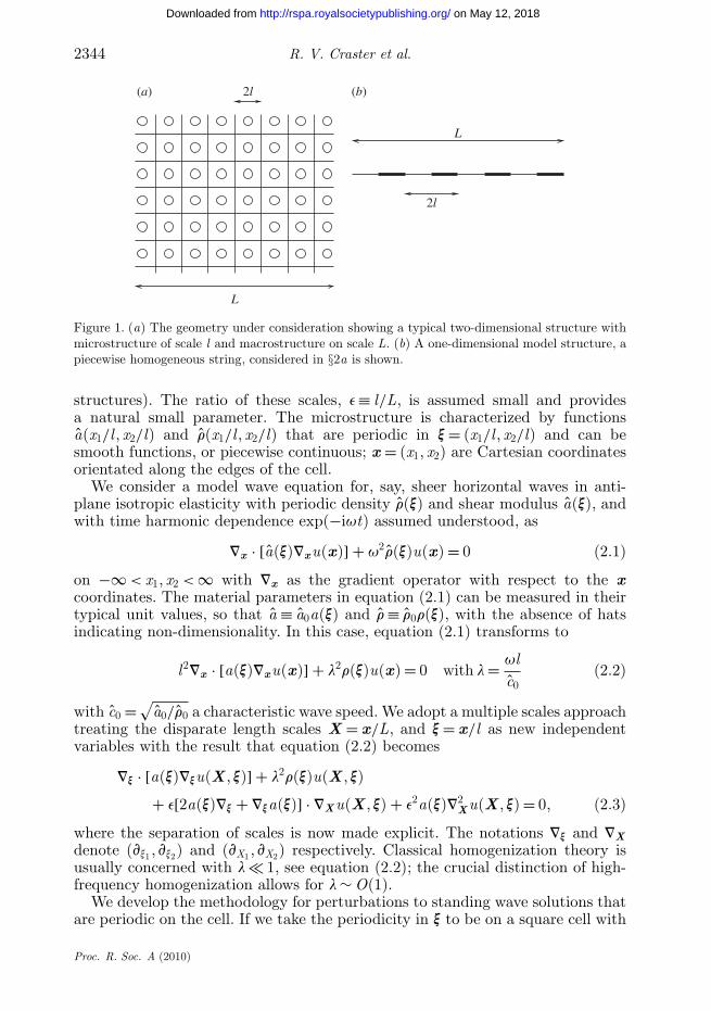
For generality, we consider a regular periodic structure composed of inclusionsand a matrix material. The inclusions are defined on a short scale l , that of themicrostructure, whereas the overall problem is considered on a macroscale L thatcan be thought of as a typical wavelength dominating the dynamic response, oran overall dimension of the structure (see figure 1 for an illustration of typical





2l(a) (b)

L

2l

L

Figure 1. (a) The geometry under consideration showing a typical two-dimensional structure withmicrostructure of scale l and macrostructure on scale L. (b) A one-dimensional model structure, apiecewise homogeneous string, considered in §2a is shown.

structures). The ratio of these scales, e ≡ l/L, is assumed small and providesa natural small parameter. The microstructure is characterized by functionsa(x1/l , x2/l) and r(x1/l , x2/l) that are periodic in x = (x1/l , x2/l) and can besmooth functions, or piecewise continuous; x = (x1, x2) are Cartesian coordinatesorientated along the edges of the cell.

We consider a model wave equation for, say, sheer horizontal waves in anti-plane isotropic elasticity with periodic density r(x) and shear modulus a(x), andwith time harmonic dependence exp(−iut) assumed understood, as

Vx · [a(x)Vxu(x)] + u2r(x)u(x) = 0 (2.1)

on −∞ < x1, x2 < ∞ with Vx as the gradient operator with respect to the xcoordinates. The material parameters in equation (2.1) can be measured in theirtypical unit values, so that a ≡ a0a(x) and r ≡ r0r(x), with the absence of hatsindicating non-dimensionality. In this case, equation (2.1) transforms to

l2Vx · [a(x)Vxu(x)] + l2r(x)u(x) = 0 with l = ulc0

(2.2)

with c0 = √a0/r0 a characteristic wave speed. We adopt a multiple scales approach

treating the disparate length scales X = x/L, and x = x/l as new independentvariables with the result that equation (2.2) becomes

Vx · [a(x)Vxu(X , x)] + l2r(x)u(X , x)

+ e[2a(x)Vx + Vxa(x)] · VXu(X , x) + e2a(x)V2Xu(X , x) = 0, (2.3)

where the separation of scales is now made explicit. The notations Vx and VXdenote (vx1 , vx2) and (vX1 , vX2) respectively. Classical homogenization theory isusually concerned with l � 1, see equation (2.2); the crucial distinction of high-frequency homogenization allows for l ∼ O(1).

We develop the methodology for perturbations to standing wave solutions thatare periodic on the cell. If we take the periodicity in x to be on a square cell with





−1 ≤ xi ≤ 1, for i = 1, 2, then periodicity conditions are to be taken in x along theedges of the cell, namely

u|x1=1 = u|x1=−1, u|x2=1 = u|x2=−1 (2.4)

and

ux1 |x1=1 = ux1 |x1=−1, ux2 |x2=1 = ux2 |x2=−1. (2.5)

The corresponding solution u(X , x) will be periodic in x, but not necessarily in X .One can replace these periodicity conditions along one or both spatial dimensionswith special ‘out-of-phase’ boundary conditions. These anti-periodic boundaryconditions lead to solutions that are periodic across two cells in the appropriatedirection(s) of x. For the sake of clarity, we specialize the two-dimensionalderivations to the case periodic in both x1 and x2 for which equations (2.4)and (2.5) apply. We illustrate the application and consequences of anti-periodicboundary conditions only for the one-dimensional case presented in §2a.

Next, we adopt the ansatz:

u(X , x) = u0(X , x) + eu1(X , x) + e2u2(X , x) + · · · , l2 = l20 + el2

1 + e2l22 + · · · .

(2.6)

Each ui(X , x) for i = 1, 2, . . ., is periodic in x, cf. equations (2.4) and (2.5).This ansatz assumes variation at both the microscale and macroscale evenat leading order, as opposed to the classical homogenization theory for whichu0(X , x) ≡ u0(X).

Substituting equation (2.6) into equation (2.3), and equating to zero thecoefficients of individual powers of e, we obtain a hierarchy of equations forui(X , x) and li with associated boundary conditions from the periodicity in x.This hierarchy is resolved from the lowest order up. At the lowest order, weobtain an eigenvalue problem for

Vx · [a(x)Vxu0] + l20r(x)u0 = 0 (2.7)

subject to the appropriate periodicity boundary conditions. This gives rise toa discrete spectrum of eigenvalues l2

0 for which there is no phase shift across aperiod of the structure and standing wave is formed. If we fix a simple eigenvaluel0, then the corresponding eigenmode is of the form

u0(X , x) = f0(X)U0(x, l0), (2.8)

where U0(x, l0) is a periodic function of x, and f0(X) remains to be determined;we introduce l0 into the argument of the periodic function to emphasize that itdepends upon the frequency l0. This leading order solution is exactly periodic onthe cell, hence conforming to the commonly used notion of the unit cell resonance(or microresonance). Notably, the case of coincident eigenvalues can also arise andis discussed in the simpler context for one-dimensional structures in the followingsection. Generally, the leading order problem would need to be solved numerically,as is the case in classical homogenization. As we desire the corrections l2

1, l22 and

the function f0(X), we continue with the hierarchy.





At next order, the equation for u1(X , x) is

Vx · [a(x)Vxu1] + l20r(x)u1 = −VX f0 · [2a(x)VxU0 + U0Vxa(x)] − f0l2

1r(x)U0 (2.9)

and we now invoke an orthogonality condition that involves multiplyingequation (2.9) by U0 and integrating over the periodic cell in x. This yields

∫∫S

(U0Vx · [a(x)Vxu1] + l2

0r(x)U0u1)dS

= −VX f0 ·∫∫

SVx[a(x)U 2

0 ] dS − f0l21

∫∫S

r(x)U 20 dS , (2.10)

where∫∫

S denotes integration over the cell. Using a corollary to the divergencetheorem, the first integral on the right-hand side is converted to an integral alongthe edges of the cell, and thereafter we use periodicity of a(x) and U0 and itvanishes. We now subtract the integral of equation (2.7), multiplied by u1/f0,over the cell, from equation (2.10), which results in

∫∫S(U0Vx · [a(x)Vxu1] − u1Vx · [a(x)VxU0]) dS = −f0l2

1

∫∫S

r(x)U 20 dS . (2.11)

Using Green’s second identity, the left-hand side becomes

∫vS

a(x)(

U0vu1

vn− u1

vU0

vn

)ds, (2.12)

where vS is the boundary of region S and n is the outward pointing normal. Fromperiodicity in x of U0, u1 and a, this integral vanishes. Thus, the only non-zeroterm is that multiplying l2

1; therefore, l1 must be identically zero. An explicitsolution for u1(X , x), from equation (2.9), with x restricted to be in the cell S , isfound as

u1(X , x) = f1(X)U0(x, l0) + VX f0(X) · [V 1(x, l0) − xU0(x, l0)], (2.13)

where the coefficient, f1, of the homogeneous solution does not appear, to leadingorder, in the final result and plays no further role here. The vector functionV 1 = (V (1)

1 , V (2)1 ) satisfies the leading order equation (2.7), that is,

Vx · [a(x)Vx]V 1 + l20r(x)V 1 = 0, (2.14)

i.e. each component of V 1 is the non-doubly periodic solution of equation (2.7)linearly independent of U0(x, l0). Notably u1(X , x) must be periodic in x; however,both terms in the square brackets of equation (2.13) are not. Therefore, we selecteach individual component of V 1 to be periodic along one of the xi and thenchoose its boundary conditions along the other xj , j �= i, in such a way thatconditions (2.4) and (2.5) are enforced; the solution can then be periodically





continued to the full structure. We set V (1)1 (x, l0) to have periodicity in x2 and

then periodicity of u1 in x1 results in

V (1)1 |x1=1 − V (1)

1 |x1=−1 = 2U0|x1=1 (2.15)

and

V (1)1x1

|x1=1 − V (1)1x1

|x1=−1 = 2U0x1 |x1=1. (2.16)

Thus, V (1)1 (x, l0) is a periodic function in x2 that must be found by solving

the inhomogeneous boundary value problem given by equation (2.14) subjectto boundary conditions consistent with equations (2.15) and (2.16), as well asequations (2.4)2 and (2.5)2.

Similarly, we take V (2)1 (x, l0) to be a solution of equation (2.14) periodic in x1

with boundary conditions

V (2)1 |x2=1 − V (2)

1 |x2=−1 = 2U0|x2=1 (2.17)

and

V (2)1x2

|x2=1 − V (2)1x2

|x2=−1 = 2U0x2 |x2=1. (2.18)

The second-order equation for u2(X , x) is

Vx · [a(x)Vxu2] + l20r(x)u2 = −a(x)U0V2

X f0 − [2a(x)Vx + Vxa(x)] · VXu1

− l22r(x)f0U0 (2.19)

and this contains both f0(X) and the correction, l22, to the eigenvalue l2

0.Invoking an orthogonality condition, as at the previous order, by multiplyingequation (2.19) by U0, subtracting equation (2.7) times u2/f0 from it, andintegrating the result over the cell yields an eigenvalue problem for f0 and l2

2as the homogenized partial differential equation

Tijv2f0

vXivXj+ l2

2f0 = 0, with Tij = tij∫∫S r(x)U 2

0 dSfor i, j = 1, 2. (2.20)

The components of the matrix tij are given by

t11 = −2∫ 1

−1[a(x)U 2

0 ]x1=1 dx2 +∫∫

S(2a(x)V (1)

1x1+ ax1(x)V

(1)1 )U0 dS , (2.21)

t12 = t21 = 12

∫∫S

(2a(x)(V (1)

1x2+ V (2)

1x1) + ax2(x)V

(1)1 + ax1(x)V

(2)1

)U0 dS (2.22)

and t22 = −2∫ 1

−1[a(x)U 2

0 ]x2=1 dx1 +∫∫

S(2a(x)V (2)

1x2+ ax2(x)V

(2)1 )U0 dS . (2.23)

Thus, given a particular structure, we solve the leading order equation (2.7) todetermine l0, U0(x, l0). Then, solve equation (2.14), with boundary conditions(2.15)–(2.18) and periodicity, to find V 1(x, l0). Given these quantities, thedifferential eigenvalue problem (2.20) is formed, and thus l2 identified.





We now specialize to one-dimensional or quasi-one-dimensional problems forwhich this scheme is more readily applied and for which some explicit details areimmediately apparent.

(a) One-dimensional periodic media

Assuming a(x) is constant, then for one-dimensional structures equation (2.2)simplifies to

l2d2udx2

+ l2 uc2(x)

= 0, with l = ulc0

, (2.24)

where we define c2(x) = a/r(x). The assumption that a(x) is constant inequation (2.24) is not essential as any homogeneous second-order differentialequation can be transformed into this form by an appropriate change of variables.

The independent variables are now X = x/L, x = x/l , and the solution u(X , x)will be periodic, or anti-periodic, in x, but not necessarily in X . The two-scalesapproach yields

v2uvx2

+ 2ev2u

vxvX+ e2 v2u

vX 2+ l2

c2(x)u = 0. (2.25)

This equation is solved subject to either x-periodicity conditions u(X , 1) =u(X , −1) and ux(X , 1) = ux(X , −1) or, what we have named, anti-periodicityconditions u(X , 1) = −u(X , −1) and ux(X , 1) = −ux(X , −1), which actually resultin the solutions being x-periodic across two cells. As we shall see shortly, these twocases correspond to standing waves that are either in-phase or completely out-of-phase at the end of each cell and, in Floquet–Bloch theory, to wavenumberssituated at the opposite ends of the Brillouin zone.

The separation of scales is loosely analogous to the long-wave high-frequencyasymptotics outlined for infinite, deformed, waveguides (Berdichevski 1983;Kaplunov et al. 1998; Le 1999) and this analogy can be pursued to obtain aphysical interpretation of the results and this is discussed in §§2b and 4. Asin the two-dimensional theory, we form a hierarchy of equations to be solvedorder-by-order. To leading order

u0xx + l20

c2(x)u0 = 0, (2.26)

and if l0 is a simple eigenvalue of the problem with an appropriate set of boundaryconditions, then

u0(x, X) = f0(X)U0(x, l0). (2.27)

In the periodic case, U0(1, l0) = U0(−1, l0), U0x(1, l0) = U0x(−1, l0) and inthe anti-periodic case, U0(1, l0) = −U0(−1, l0), U0x(1, l0) = −U0x(−1, l0). FromFloquet theory, all band gaps present in the Bloch spectra of equation (2.26) arebound by the eigenvalues corresponding to periodic or anti-periodic solutions.Hence, the high-frequency asymptotics developed here are expected to provideaccurate description of the solution’s band gap structure in a wide rangeof problems.





To next order

u1xx + l20

c2(x)u1 = −2u0xX − l2

1

c2(x)u0 (2.28)

with the compatibility condition giving l1 = 0. The solution is

u1(X , x) = f0X [AW1(x, l0) − xU0(x, l0)] + f1(X)U0(x, l0), (2.29)

where W1(x, l0) is a non-periodic solution of the leading order equation and

A = 2U0(1, l0)W1(1, l0) ∓ W1(−1, l0)

(2.30)

with the upper (lower) sign being for the periodic (anti-periodic) case and theconstant A is chosen to enforce that behaviour. At next order,

u2xx + l20

c2(x)u2 = − l2

2

c2(x)u0 − u0XX − 2u1xX (2.31)

with the compatibility condition giving

Tf0XX + l22f0 = 0, (2.32)

where the coefficient T is

T = 2

(−U 20 (1, l0) + A

∫1−1 U0W1x dx∫1

−1 U 20 /c2(x) dx

). (2.33)

The differential eigenvalue problem (2.32) then encapsulates the essentialphysics on the macroscale and the correction to the frequency squared, l2

2, isits eigenvalue.

If the leading order solution has U0(±1, l0) = 0, then equation (2.29) is notvalid; however, this is easy to overcome with equation (2.33) replaced by

T = 2A∫1

−1 U0W1x dx∫1−1 U 2

0 /c2(x) dx, (2.34)

where A = 2U0x(1, l0)/[W1x(1, l0) ∓ W1x(−1, l0)] and the non-periodic functionW1 satisfies the Dirichlet conditions, W1(±1, l0) = 1 (or any non-zero constant).

A degeneracy occurs whenever l0 is not a simple eigenvalue, as the leadingorder solution (2.26) must consist of two linearly independent periodic solutions

u0(x, X) = f (1)0 (X)U (1)

0 (x, l0) + f (2)0 (X)U (2)

0 (x, l0). (2.35)

The compatibility condition for the first-order term then gives two coupledordinary differential equations (ODEs) for f (1,2)

0 from which the eigenvaluecorrection l2

1 is obtained; the correction to the eigenvalue is now linear ratherthan quadratic. The coupled equations are

f (i)0X

∫ 1

−1U (j)

0 U (i)0x dx + l2

1

∫ 1

−1

(f (j)0 U (j)2

0 + f (i)0 U (i)

0 U (j)0

) dx

c2(x)= 0 (2.36)

for i, j = 1, 2 and j �= i.





The asymptotic model (2.32) is not uniform in the sense that when materialparameters are continuously varied, such that two eigenvalues approach oneanother, one has then to switch to the model equations (2.36). Examples fromthe waveguide theory suggest that it is possible to construct uniformly validcomposite expansions (Moukhomodiarov et al. in press) to overcome this.

(b) Analogy with homogeneous waveguides

Placing equation (2.32) in dimensional form

l2Td2f0dx2

+ (l2 − l20)f0 = 0, (2.37)

then this equation governs the one-dimensional long-wave motion of a periodicmedium near the resonance frequencies of a cell. It may be subject to macroscopicboundary conditions along the edges and may also involve inhomogeneous termson the right-hand side corresponding to edge and surface loadings, see Kaplunovet al. (1998) and references therein.

The long-wave equation (2.37) may be interpreted as describing a homogeneousstring attached to an elastic foundation. Although the microscale problem isgoverned by a Helmholtz equation with periodic coefficients, equation (2.24), theproposed model cannot be formally identified as a Helmholtz equation with anaveraged wave speed, which contrasts with traditional homogenization theory. Atthe same time, the model does not contain microscale variables operating onlywith long-scale phenomena. It is worth noting that non-local equations are alsoknown to occur as homogenized limits for certain high-contrast composite media(Cherednichenko et al. 2006).

As we have mentioned earlier, the model represents an analogue of the high-frequency long-wave theories for elastic and acoustic homogeneous waveguides(e.g. Kaplunov et al. 1998; Gridin et al. 2005). In fact, the problem on a cell (2.26)corresponds to one on the transverse cross section of a thin rod, plate or a shell.In this case, the cell size l in equation (2.24) corresponds to the half thickness andthe cell eigenvalue l0 corresponds to a thickness resonance frequency. A similaranalogy also occurs in conventional homogenization theory, which is, in a sense,a counterpart of the classical low-frequency theories for rods, plates and shellsassociated with the names of Euler, Bernoulli, Kirchhoff and Love (e.g. Love 1944;Landau & Lifshitz 1970; Graff 1975). The discussion above is also applicable totwo-dimensional periodic media.

3. Illustrative examples

To illustrate the efficacy of this approach, we turn our attention to some examples.The first example, a periodic piecewise homogeneous material, has the advantageof being explicitly solvable and serves to illustrate typical features of Blochwaves and pass-stop bands in periodic media. For some parameters, double rootsoccur allowing this feature to also be explored. This example is extended byintroducing a parameter leading to the formation of a low-frequency stop band,hence allowing us to compare and contrast the high-frequency theory with a





traditional low-frequency homogenization. Our last example is of a string witha periodic density that leads to Mathieu’s equation, allowing us to present anon-trivial application of our asymptotics.

(a) Periodic piecewise homogeneous media

For a material with piecewise constant variation in c(x),

c(x) =⎧⎨⎩

1r

for 0 ≤ x < 1

1 for − 1 ≤ x < 0(3.1)

for r a positive constant, an exact solution is readily obtained. Floquet–Bloch conditions (Brillouin 1953; Kittel 1996) are set at x = ±1; so u(1) =exp(i2ke)u(−1) and ux(1) = exp(2ike)ux(−1), the solution and its derivatives arecontinuous at x = 0, and k is the Bloch parameter. The dispersion relation relatingfrequency, l, to Bloch parameter, k, is

2r[cos l cos rl − cos 2ek] − (1 + r2) sin l sin rl = 0. (3.2)

This dispersion relation was seemingly first obtained by Kronig & Penney (1931)for electrons in crystal lattices; it also naturally appears in many guises in one-dimensional photonic and phononic crystals (with layers of infinite height), e.g.Movchan et al. (2002) and Adams et al. (2008). There are an infinite numberof discrete eigenfrequencies, l(k), to the dispersion relation that we denote asl(n) with n = 0, 1, 2 . . . ordered from the lowest curve upward; typical Blochspectra are shown in figure 2. The asymptotic technique we describe extractsthe behaviour of the dispersion curves near l

(n)0 , which is the frequency at the

edge of the Brillouin zone where k = 0. The standing waves that occur whenk = 0 correspond to solutions periodic across each elementary cell of width 2e.The other end of the Brillouin zone is at 2ek = p and corresponds to standingwaves out-of-phase across the cell, the anti-periodic solutions that are periodicon a double cell and the frequencies at which these occur are denoted by l

(n)p .

The asymptotics we develop are valid near each l(n)p and all l

(n)0 except the

low-frequency fundamental mode passing through l(0)0 = 0. This mode is the one

described by classical homogenization, whose characterization is straightforward,l

(0)0 ∼ 2ek/

√2(1 + r2), cf. equation (3.14), at b = 0, which corresponds to

the substitution ⟨1c2

⟩= 1

2

∫ 1

−1

1c2(x)

dx (3.3)

in equation (2.24). We compare the classical philosophy with the high-frequencytheory at the end of §3b.

We now turn to the asymptotic procedure. The leading order solution isdetermined as

U0(x, l(n)q ) =

{sin rl

(n)q x + p cos rl

(n)q x for 0 ≤ x < 1

r sin l(n)q x + p cos l

(n)q x for − 1 ≤ x < 0

(3.4)





0 1 2 3

11

12

13

14(b)

λ

1 2 30

2

4

6

8

10

12

14

16

18

20(a)

2ek

λ

10−1 10010−3

10−2

10−1

100(c)

2ek

λ(3) −

λ 0(3)

Figure 2. (a) The dispersion curves from equation (3.2), for r = 1/4, shown across the Brillouinzone. The solid line is from the numerical solution, the asymptotics for k → 0 are representedby the dashed curve and that for 2ek → p are by the dotted curve. Asymptotics for the doubleroot are shown as dot–dashed lines. (b) The detail for the Bloch spectra at the double root at

l(4)p = l

(5)p = 4p with the asymptotics shown as the dot–dashed lines. (c) Plots l

(3) − l(3)0 on log–

log axes to illustrate the accuracy: numerics are given by the solid line and the asymptotics by thedashed line.

for l(n)q = l

(n)0 , l

(n)p and p = (r sin l

(n)q ± sin rl

(n)q )/(cos l

(n)q ∓ cos rl

(n)q ) with the

upper, lower signs for q = 0, p, respectively. We also need a linearly independentsolution, which does not satisfy periodicity or anti-periodicity conditions atx = ±1, W1(x, l

(n)q ). We take it as

W1(x, l(n)q ) =

{sin rl

(n)q x for 0 ≤ x < 1

r sin l(n)q x for − 1 ≤ x < 0.

(3.5)

Note that W1 can be taken to be any solution of the leading order equation withfixed l0, which is neither periodic nor anti-periodic. Once W1 is found, it can bere-used in the asymptotics for either end of the Brillouin zone.

Substituting these into equation (2.33) gives T0 and Tp, that is, the T valuesassociated with the periodic and anti-periodic solutions. These two are writtenusing a single formula as

T (n)q = ±4l

(n)q

sin l(n)q sin l

(n)q r

(r sin l(n)q ∓ sin rl

(n)q )(cos l

(n)q ∓ cos rl

(n)q )

, (3.6)

where we append a subscript to T to denote its dependence upon l(n)q and T (n)

0 ;(T (n)

p ) is the value with the upper (lower) sign and l(n)q = l

(n)0 (l(n)

p ).





We now turn our attention to the ODE for f0, namely equation (2.32), andnote that the Floquet–Bloch conditions lead to u(X + 2e, x) = exp(2iek)u(X , x).For the periodic case in x, this forces f0(X) = exp(ikX). Thus, we connect theBloch parameter with the frequency, found from equation (2.32), via Tk2 = l

(n)22

and deduce that

l(n) ∼ l(n)0 + e2

2l

(n)22

l(n)0

+ · · · = l(n)0 + e2

2T (n)

0 k2

l(n)0

+ · · · . (3.7)

Similarly, in the anti-periodic case, we deduce f0(X) = exp(i(k − p)X) and

l(n) ∼ l(n)p + e2

2T (n)

p (k − p)2

l(n)p

+ · · · . (3.8)

The same results are found directly by expanding the exact dispersion relation(3.2), thereby validating the asymptotic scheme for an example that can beexplicitly analysed; the advantage of the asymptotic procedure is that it isapplicable even when the dispersion relation is unwieldy or unavailable. As thederived expansion makes no specific assumptions about the form of the leadingorder solution, it is valid for arbitrary volume fractions, although the resultingnumerical accuracy at fixed wavenumbers may vary.

We order the eigenvalues for n = 0 . . . ∞ from lowest to highest in magnitudeand note that the asymptotics do not apply to the lowest eigenvalue, l

(0)0 ,

which passes through the origin and which have been approached separately,but is accurate for high frequencies. Figure 2 shows the band gap structure andassociated asymptotics that emanate from the frequencies at the edges of theBrillouin zone. The quadratic corrections are highly accurate even for valuesof k far away from the edges of the zone and this is shown in figure 2c. Adouble root occurs at l

(4)p = l

(5)p and the asymptotics shown in figure 2b are the

linear corrections from equation (2.36). An essential ingredient of the asymptoticprocedure is the identification of the leading order solutions U0(x, l

(n)q ) for the

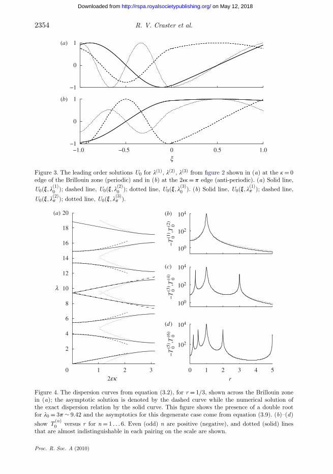
standing waves across the structure. Typical curves are shown in figure 3 for theU0 at each edge of the Brillouin zone, and as the frequency increases the solutionsgain more spatial structure.

The degenerate case of a double root is again illustrated in figure 4. In figure 4b,we note that T (n)

0 diverges for some values of r and further analysis showsthat these values correspond to the cases of a double root for l

(n)q , which occur

whenever r = 1/m, m (for integer m). For instance, for r = 1/3, as in the figure,l

(4),(5)0 = 3p, and there is no band gap (as shown in figure 4a). The asymptotics

are extracted using the coupled equations (2.36) as

l(3),(4) ∼ 3p ± 3ek√5

+ · · · (3.9)

and as noted earlier, the correction is linear in k rather than the quadraticbehaviour found for distinct roots. A similar double root behaviour occurs atthe other end of the Brillouin zone, and is shown in figure 2b, together with theasymptotics from equation (2.36).





−1

0

1(a)

(b)

−1.0 −0.5 0 0.5 1.0−1

0

1

x

Figure 3. The leading order solutions U0 for l(1), l(2), l(3) from figure 2 shown in (a) at the k = 0edge of the Brillouin zone (periodic) and in (b) at the 2ek = p edge (anti-periodic). (a) Solid line,

U0(x, l(1)0 ); dashed line, U0(x, l

(2)0 ); dotted line, U0(x, l

(3)0 ). (b) Solid line, U0(x, l

(1)p ); dashed line,

U0(x, l(2)p ); dotted line, U0(x, l

(3)p ).

1 2 30

2

4

6

8

10

12

14

16

18

20(a) (b)

(c)

(d)

2ek

l

100

102

104

100

102

104

0 1 2 3 4 5

102

104

r

−T

0(5) ,T

0(6)

−T

0(3) ,T

0(4)

−T

0(1) ,T

0(2)

Figure 4. The dispersion curves from equation (3.2), for r = 1/3, shown across the Brillouin zonein (a); the asymptotic solution is denoted by the dashed curve while the numerical solution ofthe exact dispersion relation by the solid curve. This figure shows the presence of a double rootfor l0 = 3p ∼ 9.42 and the asymptotics for this degenerate case come from equation (3.9). (b)–(d)

show T (n)0 versus r for n = 1 . . . 6. Even (odd) n are positive (negative), and dotted (solid) lines

that are almost indistinguishable in each pairing on the scale are shown.





(b) A model structure with non-uniform low-frequency behaviour

The piecewise homogeneous structure has its lowest Bloch spectra curvel(0)(k) passing through l(0)(0) = l

(0)0 = 0 and as it passes exactly through zero,

this low-frequency mode is not captured within our asymptotics. The classicalhomogenization theory describes the behaviour of this low-frequency curve bothwhen it passes through zero and when an extra (small) parameter exists, as inthe example to be considered in this section, that moves the curve upward toexpose a low-frequency stop band. We now consider an adaption of the piecewisehomogeneous model that allows us to contrast the classical theory with ourhigh-frequency asymptotic approach for this lowest curve of the Bloch spectra.

We previously mentioned that the model equations obtained during thehigh-frequency homogenization of one-dimensional periodic structures describevibration of an effective homogeneous string on a Winkler foundation. In thiscontext, it is instructive to study homogenization of a periodically piecewisehomogeneous string on a Winkler foundation. This setup also describes a stripedwaveguide (Adams et al. 2008, 2009) of finite thickness with Dirichlet, Neumannor impedance (Robin) boundary conditions along the guide walls. In both cases,the governing equation is equivalent to

l2d2udx2

− b2u + l2

c2(x/l)u = 0. (3.10)

The additional term −b2u corresponds to the constant elastic restoring parameterin the Winkler model, or to the separation constant that is related to thetransverse mode number for the striped waveguide, and its presence createsa low-frequency stop band. The dispersion relation is a minor adjustment ofequation (3.2) to

2k1k2(cos k1 cos k2 − cos 2ek) − (k21 + k2

2 ) sin k1 sin k2 = 0 (3.11)

with k21 = l2 − b2, k2

2 = r2l2 − b2. For non-zero b, there is no fundamental modepassing through the origin in the Bloch spectra for this model; hence, high-frequency asymptotics are capable of describing every Floquet–Bloch mode. Thetwo-scales analysis goes through precisely as before with l

(n)0 deduced from

equation (3.11) with k = 0. The asymptotic correction l(n)2 is deduced from

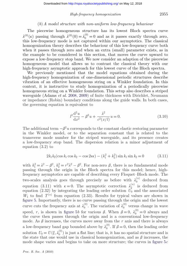
equation (2.32) by integrating the leading order solution U0 and the associatedW1 to find T (n) from equation (2.33). Results for typical values are shown infigure 5. Importantly, there is no curve passing through the origin and the lowestcurve cuts the frequency axis at l

(0)0 . The variation of l

(0)0 versus change in wave

speed, r , is shown in figure 5b for various b. When b = 0, l(0)0 = 0 always and

the curve then passes through the origin and is a conventional low-frequencymode. As b increases, the curves move away from the r axis and there is alwaysa low-frequency band gap bounded above by l

(0)0 . If b = 0, then the leading order

solution U0 = U (x, l(0)0 ) is just a flat line; that is, it has no spatial structure and is

the state that one would use in classical homogenization, and as b increases, themode shape varies and begins to take on more structure; the curves in figure 5c





1 2 30

1

2

3

4

5

6

7

8

9

10(a) (b)

(c)

2ek

λ

−1 0 10.90

0.95

1.00

x

U0

2 40

0.5

1.0

1.5

r

l0(0)

Figure 5. The dispersion curves for the piecewise homogeneous string on a Winkler foundation.(a) is for r = 1/4, b = 1 showing the absence of the fundamental mode and the curves from the fullnumerics (solid) versus the asymptotics (dashed). (b) The variation of the lowest frequency cut-off

at k = 0, namely l(0)0 , versus the change in wave speed r for various values of b. (c) The variation

in the leading order solution, U0(x, l(0)0 ) as b increases for fixed r : r = 1.5 in (c). (b,c) Solid line,

b = 0.25; dashed line, b = 0.5; dot-dashed line, b = 0.75; dotted line, b = 1.

are normalized to have max(|U0|) = 1. Further details of the Bloch spectra for thisexample are in Adams et al. (2008, 2009) together with the details of numericalschemes and other asymptotic techniques that can be applied.

The lowest curve of the Bloch spectra can be approximated using quasi-static distributions along the cell corresponding to classical homogenization. Thisrequires low frequencies and b ∼ eb for which the appropriate asymptotic orderingis that

u(X , x) = u0(X , x) + eu1(X , x) + · · · , l2 = e2l22 + · · · . (3.12)

The leading order equation then gives u0(X , x) = f0(X), which is uniform alongthe cell; that is, it does not depend upon the small-scale x at all and thisdifference, and the scaling of l, is a major difference between the high- and low-frequency models. The function f0(X), from the second-order equation, satisfiesthe differential eigenvalue problem

f0XX − b2f0 + f0l2

2

2

∫ 1

−1

1c2(x)

dx = 0. (3.13)





1 2 30

0.5

1.0

1.5

2.0b = 0.5

b = 0.25

50

1

2

3

4

5

0 1 2 31.0

1.5

2.0

2.5

3.0(a) (b) (c)

λ

b = 2

b = 1

2ek 2ek b

l0(0)

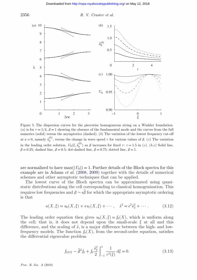
Figure 6. A comparison of the low-frequency homogenization formula (3.14) (dotted lines) withthe numerical solution (solid) and the high-frequency asymptotics (dashed). In all panels, r = 1/4and in (a), we show l(0) for b = 2 and b = 1. Likewise in (b) but for b = 0.5 and b = 0.25. (c)

The variation in l(0)0 versus b predicted by the low-frequency asymptotics (dotted) and from the

numerics (solid).

In this classical model, the inverse-squared wave speed c is replaced inequation (3.10) by an averaged quantity 〈1/c2〉, defined in equation (3.3), andhomogenization replaces the variable wave speed by this averaged quantity. Thehigh-frequency asymptotics that we employ are fundamentally different; theyare not limited by low-frequency quasi-static variations along the cell and donot simply replace periodic inverse wave speed squared by a constant. Theasymptotics take the solution of the standing wave and construct an effectiveparameter, T , as an integral over x that involves the wave speed and the standingwave solution.

Returning to the problem at hand, the Bloch conditions yield f0(X) = exp(ikX)and thus this lowest curve is given asymptotically in the low-frequency limit as

l(0)2 ∼ 4b2 + (2ek)2

2(1 + r2)(3.14)

for b � 1 and small k. We compare this result with the high-frequency asymptoticsin figure 6; from (b) and (c), we see that at low frequencies, equivalently smallb, equation (3.14) performs well in predicting the dispersion curves. The high-frequency theory is applicable for small k but diverges from the numerics soonerthan the low-frequency results. For large b, figure 6a, the low-frequency theorydrifts away from the solid curve, and becomes inaccurate, and the high-frequencyresults remain accurate and are so over a longer domain in k.

(c) A continuous periodic variation

We now consider a string with periodic variation in density that leads tothe wave speed c−2(x) = a − 2Q cos 2x, where a, Q are positive constants; thisvariation gives the classical Mathieu equation (Abramowitz & Stegun 1964;McLachlan 1964) and to more readily connect with the standard theory for that





0.5 1.00

1

2

3

4

5

6

7

8

ek

l

(a) (b)

(c)

−1.0

−0.5

0

0.5

1.0

0 1 2 3

–0.5

0

0.5

1.0

x

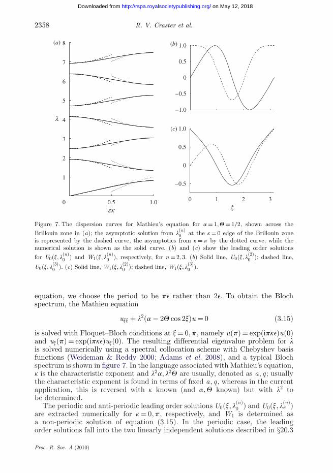
Figure 7. The dispersion curves for Mathieu’s equation for a = 1, Q = 1/2, shown across theBrillouin zone in (a); the asymptotic solution from l

(n)0 at the k = 0 edge of the Brillouin zone

is represented by the dashed curve, the asymptotics from k = p by the dotted curve, while thenumerical solution is shown as the solid curve. (b) and (c) show the leading order solutions

for U0(x, l(n)0 ) and W1(x, l

(n)0 ), respectively, for n = 2, 3. (b) Solid line, U0(x, l

(2)0 ); dashed line,

U0(x, l(3)0 ). (c) Solid line, W1(x, l

(2)0 ); dashed line, W1(x, l

(3)0 ).

equation, we choose the period to be pe rather than 2e. To obtain the Blochspectrum, the Mathieu equation

uxx + l2(a − 2Q cos 2x)u = 0 (3.15)

is solved with Floquet–Bloch conditions at x = 0, p, namely u(p) = exp(ipke)u(0)and ux(p) = exp(ipke)ux(0). The resulting differential eigenvalue problem for lis solved numerically using a spectral collocation scheme with Chebyshev basisfunctions (Weideman & Reddy 2000; Adams et al. 2008), and a typical Blochspectrum is shown in figure 7. In the language associated with Mathieu’s equation,k is the characteristic exponent and l2a, l2Q are usually, denoted as a, q; usuallythe characteristic exponent is found in terms of fixed a, q, whereas in the currentapplication, this is reversed with k known (and a, Q known) but with l2 tobe determined.

The periodic and anti-periodic leading order solutions U0(x, l(n)0 ) and U0(x, l

(n)p )

are extracted numerically for k = 0, p, respectively, and W1 is determined asa non-periodic solution of equation (3.15). In the periodic case, the leadingorder solutions fall into the two linearly independent solutions described in §20.3





0.1 0.2 0.3 0.4Q Q

0.5100

102

104

(a) (b)

T

0.1 0.2 0.3 0.4 0.51.8

2.0

2.2

2.4

Figure 8. (a) and (b) show the variation of T (n)0 and l

(n)0 versus Q, for a = 1, for n = 2, 3. (a) Solid

line, −T (2)0 ; dashed line, T (3)

0 . (b) Solid line, l(2)0 ; dashed line, l

(3)0 .

of Abramowitz & Stegun (1964): one being characterized by U0(0, l(n)0 ) = 1,

U0(p, l(n)0 ) = 1, U0x(p, l

(n)0 ) = 0 (these lead to the n odd cases) and the other by

U0x(0, l(n)0 ) = 1, U0x(p, l

(n)0 ) = 1, U0(p, l

(n)0 ) = 0 (these lead to the n even cases).

The n even cases have U0(p, l(n)0 ) = 0 and the formula for T from equation (2.34)

is used. The non-periodic solution W1 is taken to have boundary conditionsW1(0, l

(n)0 ) = 0, W1(p, l

(n)0 ) = 1 for the odd case and W1(0, l

(n)0 ) = W1(p, l

(n)0 ) = 1

for the even case. The anti-periodic case also naturally falls into two linearindependent solutions and these too are found numerically.

Given the leading order (U0) and non-periodic (W1) solutions, the integralsfor T are evaluated numerically. The change of length of the periodic domainleads to minor changes owing to a rescaling of the domain, and after performingthis change the corrections l

(n)2 to l

(n)0 and l

(n)p are readily found and the resulting

asymptotics are shown versus the complete numerics in figure 7. The asymptoticsare highly accurate near the edges of the Brillouin zone, as illustrated in figure 7a.The curve for l(0) passes through the origin and the asymptotics for this curve nearzero are found using the classical low-frequency approach, as in equation (3.13),and l(0) ∼ ek/

√a.

The leading order solutions for U0 are shown in figure 7b with the n = 2 solutionclearly zero at the ends of the domain, and the solutions chosen for W1 are shownin figure 7c. Figure 8a,b shows that as Q → 0, physically the material variationdecreasing, the values of T (n)

0 shown increase dramatically and the differencebetween the consecutive l

(n)0 decreases until the band gap disappears and one

obtains a double root; the figure shows the results for n = 2, 3 and similar resultshold for higher n and at the other end of the Brillouin zone.

4. Concluding remarks

The high-frequency asymptotic theory that we present extends classicalhomogenization, breaking free of the static or low-frequency limitation on thesolution variation along the cell. The examples chosen show that by perturbingaway from the standing wave solutions, the Bloch spectra are identified through a





simple differential eigenvalue problem (2.20) in two-dimension and (2.32) in one-dimension. This differential eigenvalue problem is characterized by a constantparameter whose definition involves the integrations over the short scale of theperiodic cell and this short scale plays no further role in the problem; themethodology differs from conventional homogenization theory in several criticalways, and the main one is that the basic state has spatial dependence andso the integrated quantities are not simply averaged wave speeds or simpleaveraged quantities.

Remarkably, the final ODE equation (2.32) is exactly that which arises inthe high-frequency long-wave asymptotics in, say, a straight acoustic waveguide(Gridin et al. 2004). Near the thickness resonance frequencies for the waveguide,i.e. near the eigenvalues of the transverse resonance problem for a homogeneouswaveguide, a wave bounces across the guide width, forming a near-standingwave that barely propagates along the guide. Therefore, despite being at highfrequency, the wavelength is long. In the periodic situation considered in thisarticle, the vision we have of the wave is that it bounces within a periodic cell ofthe structure with no phase change, or complete phase change, across the period,to leading order, again forming a standing wave barely propagating along thestructure. In both situations, the transverse resonance and standing waves, thewave about which we perturb has a large wavelength, but can occur at a highfrequency and so they are both amenable to similar asymptotic methods. A majorbenefit of having an asymptotic theory at hand is that it uncovers the physics andalso complements numerical schemes. For instance, by evaluating the parameterT directly from the standing wave solutions, it is possible to both determine thesign and estimate the value of group velocity of Bloch modes near the edges ofthe Brillouin zone.

In the long-wave high-frequency theory of waveguides, the ODE is oftenaugmented by terms that account for curvature or geometrical variations alongthe guide (Gridin et al. 2005; Kaplunov et al. 2005) and which may lead totrapping or localization phenomena. Similar adjustments to the periodic theorycan be undertaken and this approach leads to a theory identifying localizedmodes in media with weakly varying periodic behaviour. The two-scales approachoutlined in this article provides a general methodology for treating doublycontinuous periodic media, and can be extended to discrete periodic modelsconsisting of point masses and springs. Such models are commonplace in solidstate physics and they also exhibit band gap phenomena (Brillouin 1953; Kittel1996). This, and other, extensions of the theory are underway.

The authors thank NSERC (Canada) and the EPSRC (UK) for support through the DiscoveryGrant Scheme and grant EP/H021302, respectively. J.K. thanks the University of Alberta for itshospitality and support under the Visiting Scholar programme. The authors gratefully acknowledgeuseful conversations with Sebastien Guenneau, Evgeniya Nolde and Valery Smyshlyaev.

References

Abramowitz, M. & Stegun, I. A. 1964 Handbook of mathematical functions. Washington, DC:National Bureau of Standards.

Adams, S. D. M., Craster, R. V. & Guenneau, S. 2008 Bloch waves in periodic multi-layeredwaveguides. Proc. R. Soc. A 464, 2669–2692. (doi:10.1098/rspa.2008.0065)



http://dx.doi.org/doi:10.1098/rspa.2008.0065



Adams, S. D. M., Craster, R. V. & Guenneau, S. 2009 Negative bending mode curvature via Robinboundary conditions. C. R. Phys. 10, 437–446. (doi:10.1016/j.crhy.2009.03.009)

Andrianov, I. V., Bolshakov, V. I., Danishevs’kyy, V. V. & Weichert, D. 2008 Higher orderasymptotic homogenization and wave propagation in periodic composite materials. Proc. R.Soc. A 464, 1181–1201. (doi:10.1098/rspa.2007.0267)

Arbogast, T., Douglas Jr, J. & Hornung, U. 1990 Derivation of the double porosity model of singlephase flow via homogenization theory. SIAM J. Math. Anal. 21, 823–836. (doi:10.1137/0521046)

Babych, N. O., Kamotski, I. V. & Smyshlyaev, V. P. 2008 Homogenization of spectral problems inbounded domains with doubly high contrasts. Netw. Heterogen. Media 3, 413–436.

Bakhvalov, N. & Panasenko, G. 1989 Homogenization: averaging processes in periodic media.Dordrecht, MA: Kluwer.

Bakhvalov, N. S. & Eglit, M. E. 2000 Effective dispersive equations for wave propagation in periodicmedia. Doklady Math. 370, 1–4.

Bensoussan, A., Lions, J. & Papanicolaou, G. 1978 Asymptotic analysis for periodic structures.Amsterdam, The Netherlands: North-Holland.

Berdichevski, V. L. 1983 Variational principles of continuum mechanics. Moscow, Russia: Nauka.[In Russian.]

Birman, M. S. 2004 On homogenization procedure for periodic operators near the edge of aninternal gap. St Petersbg. Math. J. 15, 507–513. (doi:10.1090/S1061-0022-04-00819-2)

Birman, M. S. & Suslina, T. A. 2006 Homogenization of a multidimensional periodic ellipticoperator in a neighborhood of the edge of an internal gap. J. Math. Sci. 136, 3682–3690.(doi:10.1007/s10958-006-0192-9)

Brillouin, L. 1953 Wave propagation in periodic structures: electric filters and crystal lattices, 2ndedn. New York, NY: Dover.

Cherednichenko, K. D., Smyshlyaev, V. P. & Zhikov, V. V. 2006 Non-local homogenized limitsfor composite media with highly anisotropic periodic fibres. Proc. Roy. Soc. Edin. 136, 87–114.(doi:10.1017/S0308210500004455)

Graff, K. F. 1975 Wave motion in elastic solids. Oxford, UK: Oxford University Press.Gridin, D., Adamou, A. T. I. & Craster, R. V. 2004 Electronic eigenstates in quantum rings:

asymptotics and numerics. Phys. Rev. B 69, 155 317. (doi:10.1103/PhysRevB.69.155317)Gridin, D., Craster, R. V. & Adamou, A. T. I. 2005 Trapped modes in curved elastic plates. Proc.

R. Soc. A 461, 1181–1197. (doi:10.1098/rspa.2004.1431)Joannopoulos, J. D., Meade, R. D. & Winn, J. N. 1995 Photonic crystals, molding the flow of light.

Princeton, NJ: Princeton University Press.Kaplunov, J. D., Kossovich, L. Yu. & Nolde, E. V. 1998 Dynamics of thin walled elastic bodies.

New York, NY: Academic Press.Kaplunov, J. D., Rogerson, G. A. & Tovstik, P. E. 2005 Localized vibration in elastic structures with

slowly varying thickness. Quart. J. Mech. Appl. Math. 58, 645–664. (doi:10.1093/qjmam/hbi028)Kittel, C. 1996 Introduction to solid state physics, 7th edn. New York, NY: John Wiley & Sons.Kronig, R. L. & Penney, W. G. 1931 Quantum mechanics in crystals lattices. Proc. R. Soc. Lond. A

130, 499–531. (doi:10.1098/rspa.1931.0019)Kushwaha, M. S., Halevi, P., Dobrzynski, L. & Djafari-Rouhani, B. 1993 Acoustic band structure of

periodic elastic composites. Phys. Rev. Lett. 71, 2022–2025. (doi:10.1103/PhysRevLett.71.2022)Landau, L. D. & Lifshitz, E. M. 1970 Theory of elasticity, 2nd edn. Oxford, UK: Pergamon Press.Le, K. C. 1999 Vibrations of shells and rods. Berlin, Germany: Springer.Love, A. E. H. 1944 A treatise on the mathematical theory of elasticity. New York, NY: Dover.Mciver, P. 2007 Approximations to wave propagation through doubly-periodic arrays of scatterers.

Waves Random Complex Media 17, 439–453. (doi:10.1080/17455030701481831)McLachlan, N. W. 1964 Theory and application of Mathieu functions. New York, NY: Dover

Publications.Milton, G. W. 2002 The theory of composites. Cambridge, UK: Cambridge University Press.Moukhomodiarov, R. R., Pichugin, A. V. & Rogerson, G. A. In press. The transition between

Neumann and Dirichlet boundary conditions in isotropic elastic plates. Math. Mech. Solids.Movchan, A. B., Movchan, N. V. & Poulton, C. G. 2002 Asymptotic models of fields in dilute and

densely packed composites. London, UK: ICP Press.



http://dx.doi.org/doi:10.1016/j.crhy.2009.03.009


http://dx.doi.org/doi:10.1137/0521046

http://dx.doi.org/doi:10.1090/S1061-0022-04-00819-2

http://dx.doi.org/doi:10.1007/s10958-006-0192-9

http://dx.doi.org/doi:10.1017/S0308210500004455

http://dx.doi.org/doi:10.1103/PhysRevB.69.155317


http://dx.doi.org/doi:10.1093/qjmam/hbi028


http://dx.doi.org/doi:10.1103/PhysRevLett.71.2022




Parnell, W. J. & Abrahams, I. D. 2006 Dynamic homogenization in periodic fibre reinforced media.quasi-static limit for SH waves. Wave Motion 43, 474–498. (doi:10.1016/j.wavemoti.2006.03.003)

Poulton, C. G., McPhedran, R. C., Nicorovici, N. A., Botten, L. C. & Movchan, A. B.2001 Asymptotics of photonic band structures for doubly-periodic arrays. In IUTAM Symp.on Mechanical and Electromagnetic Waves in Structured Media (eds R. C. McPhedran,L. C. Botten & N. A. Nicorovici), pp. 227–238. New York, NY: Kluwer.

Poulton, C. G., Mcphedran, R. C., Movchan, N. V. & Movchan, A. B. In press. Convergenceproperties and flat bands in platonic crystal band structures using the multipole formulation.Waves Random Complex Media.

Rayleigh, J. W. S. 1892 On the influence of obstacles arranged in rectangular order upon theproperties of a medium. Phil. Mag. 34, 481–502.

Sanchez-Palencia, E. 1980 Non-homogeneous media and vibration theory. Berlin, Germany:Springer.

Santosa, F. & Symes, W. W. 1991 A dispersive effective medium for wave propagation in periodiccomposites. SIAM J. Appl. Math. 51, 984–1005. (doi:10.1137/0151049)

Smith, D. R., Pendry, J. B. & Wiltshire, M. C. K. 2004 Metamaterials and negative refractiveindex. Science 305, 788–792. (doi:10.1126/science.1096796)

Smyshlyaev, V. P. 2009 Propagation and localization of elastic waves in highly anisotropicperiodic composites via two-scale homogenization. Mech. Mater. 41, 434–447. (doi:10.1016/j.mechmat.2009.01.009)

Smyshlyaev, V. P. & Cherednichenko, K. D. 2000 On rigorous derivation of strain gradient effectsin the overall behaviour of periodic heterogeneous media. J. Mech. Phys. Solids 48, 1325–1357.(doi:10.1016/S0022-5096(99)00090-3)

Weideman, J. A. C. & Reddy, S. C. 2000 A MATLAB differentiation matrix suite. ACM Trans.Math. Software 26, 465–519. (doi:10.1145/365723.365727)

Zolla, F., Renversez, G., Nicolet, A., Kuhlmey, B., Guenneau, S. & Felbacq, D. 2005 Foundationsof photonic crystal fibres. London, UK: Imperial College Press.



http://dx.doi.org/doi:10.1016/j.wavemoti.2006.03.003


http://dx.doi.org/doi:10.1126/science.1096796

http://dx.doi.org/doi:10.1016/j.mechmat.2009.01.009

http://dx.doi.org/doi:10.1016/j.mechmat.2009.01.009

http://dx.doi.org/doi:10.1016/S0022-5096(99)00090-3

http://dx.doi.org/doi:10.1145/365723.365727


high-frequency homogenization for periodic...

Documents