Higgs  CP  measurements  in  di-­‐boson  decays  

Kirill  Prokofiev      

Outline  

•  Present  spin-­‐parity  measurements      

•  CP  mixing  and  anomalous  couplings    

•  Measurements  for  the  LHC  run-­‐II  and  HL-­‐LHC    

•  Beyond  the  HL-­‐LHC.  

                         page  2  

Introduc@on  

•  The  run-­‐I  of  the  LHC:    about  5  D-­‐1  at  √s  =  7  TeV  and  about  20    D-­‐1  at  √s  =  8  TeV    per  experiment.  –  Observa@on  of  the  new  resonance:  WW,  ZZ*,  γγ  (10  D-­‐1)  –  Confirma@on:  full  run-­‐I  dataset.  

 •  Spin  and  parity  measurement:  considering  spin-­‐0,1,2.  

–  Integer  spin:  decay  to  two  vector  bosons.  –  Spin-­‐1  hypothesis  is  strongly  disfavored  due  to  the  observa@on  of  

decay  to  two  on-­‐shell  photons.  

•  Direct  spin  and  parity  analyses  performed  in  both  ATLAS  and  CMS.  

                         page  3  

Spin  and  parity  analyses  •  Observed  decays  (full  LHC  run-­‐I  dataset)  and  corresponding  spin-­‐CP  analyses:  

         

               •  Combined  spin  and  parity  measurements:  

–  ATLAS:  WW+ZZ*+γγ  (Phys.  Le).  B  726  (2013),  pp.  120-­‐144)    

–  CMS:  WW+ZZ*+γγ      (arXiv:1411.3441v1)                              page  4  

ATLAS   CMS  

Significance  observed  

Spin-­‐CP  analysis  

Significance  observed  

Spin-­‐CP  analysis  

Hàγγ   7.4  σ   ✔   3.9  σ   ✔  

HàZZ(*)à4l   6.6  σ   ✔   6.7  σ   ✔  

HàWW(*)àlνlν   3.8  σ   ✔   4.0  σ   ✔  

Hàττ   4.2  σ   ?   >3  σ   ?  VH  (Hàbb)   1.4  σ   ?   2.1  σ   ?  VBF  (any)   ?   ?  

The  spin-­‐0  par@cle  •  The  absolute  majority  of  these  studies  were  based  on  direct  exclusion  of  

alterna@ve  JP  hypotheses  in  favor  of  the  JP=0+  suggested  by  the  Standard  Model.  

                     •  DØ  constraint  on  0-­‐  scenario  at  97.9%  CL  from  W/Z+bb  (DØ  Note  6406-­‐CONF);  

constraint  on  2+  scenario  at  99.9%  CL  from  W/Z+bb  (DØ  Note  6387-­‐CONF).  –  Assuming  Standard  Model  produc@on  CS  X  BR.  

                           page  5  

JP  hypotheses  ATLAS     CMS  exclusion  

Exclusion  (%CL)   channel   Exclusion  (%CL)   channel  

0-­‐   97.8   ZZ*   >99.9   ZZ*+WW  

1+   >99.9   ZZ*+WW   >99.9   ZZ*+WW  1-­‐   99.7   ZZ*+WW   >99.9   ZZ*+WW  2+m   >99.9   ZZ*+WW+γγ   >99.9   ZZ*+WW+γγ  

Phys.  Le).  B  726  (2013),  pp.  120-­‐144   CMS-­‐PAS-­‐HIG-­‐13-­‐005   CMS-­‐PAS-­‐HIG-­‐13-­‐002   arXiv:1411.3441v1  

The  spin-­‐0  par@cle  •  LHC  Run-­‐I  data:  Large  campaign  on  excluding  alterna@ve  hypotheses  in  favor  of  

the  Standard  Model  JP=0+  hypothesis.    –  CMS  has  published  pre-­‐final  run-­‐I  results,  ATLAS  analyses  are  also  

converging.    

                         page  6  Phys.  Le).  B  726  (2013),  pp.  120-­‐144  

CMS:  a  large  number  of  spin-­‐2  models  of  both  pari@es  including  scenarios  with  higher  dimension  operators.    Both  ggF  and  qq  produc@on  mechanisms.  Combined  ZZ*+WW*  exclusion  >  3.5σ  for  each  model.  

1411.3441v1  

) + 0 /

LP J

ln(L

×-2

-60-40-20

020406080

100120 CMS (7 TeV)-1 (8 TeV) + 5.1 fb-119.7 fb ZZ + WW→X

Observed Expectedσ 1± +0 σ 1± PJσ 2± +0 σ 2± PJσ 3± +0 σ 3± PJ

- 1 + 1 m+ 2 h2+ 2 h3+ 2 h+ 2 b+ 2 h6+ 2 h7+ 2 h- 2 h9- 2 h10

- 2 m+ 2 h2+ 2 h3+ 2 h+ 2 b+ 2 h6+ 2 h7+ 2 h- 2 h9- 2 h10

- 2

qq gg production productionqq

Spin-­‐0  par@cle?  •  HàZZ*à4l:  vector-­‐  

pseudo-­‐vector  admixture.  –  Ignoring  possible  Zγ*    

and  γγ*  contribu@ons.              

•  HàZZ*à4l:  Non-­‐interfering  states:  narrow  resonances  with  different  spin  and  parity  AND  nearly  degenerate  mass.  Both  spin-­‐1  and  spin-­‐2  cases.  

                         page  7  

1411.3441v1  

b2f0 0.2 0.4 0.6 0.8 1

)+ 0 /

LP J

ln(L

×-2

-20

-10

0

10

20

30

40

50

60

CMS (7 TeV)-1 (8 TeV) + 5.1 fb-119.7 fb

ZZ→ X → qq

+0Expected at 95% CLExpected at 68% CL

ObservedPJ

Expected at 95% CLExpected at 68% CL

b2f0 0.2 0.4 0.6 0.8 1

)+ 0 /

LP J

ln(L

×-2

-20

-10

0

10

20

30

40

50

60

CMS (7 TeV)-1 (8 TeV) + 5.1 fb-119.7 fb

ZZ→X

+0Expected at 95% CLExpected at 68% CL

ObservedPJ

Expected at 95% CLExpected at 68% CL

)Pf(J

0

0.1

0.2

0.3

0.4

0.5

0.6

0.7

0.8

0.9

1

m+ 2

gg production

h2+ 2

productionqq

h3+ 2

(gg acceptance)decay-only discriminants

h+ 2 b+ 2 h6+ 2 h7+ 2 h- 2 h9- 2 h10

- 2 m+ 2 h2+ 2 h3+ 2 h+ 2 b+ 2 h6+ 2 h7+ 2 h- 2 h9- 2 h10

- 2 m+ 2 h2+ 2 h3+ 2 h+ 2 b+ 2 h6+ 2 h7+ 2 h- 2 h9- 2 h10

- 2σ 1±Best fit Excluded at 95% CLExpected at 95% CLExpected at 68% CL

CMS (7 TeV)-1 (8 TeV) + 5.1 fb-119.7 fb ZZ→H

Spin-­‐0  par@cle?  

•  Hàγγ,  HàZZ*:  Direct  measurement  of  compa@bility  with  spin-­‐0  hypothesis.  –  Differen@al  cross  sec@on  as  the  func@on  of  produc@on  angle  |cos  θ*|.  –  Spin-­‐sensi@ve:  isotropic  for  spin-­‐0,  polynomial  up  to  cos2JΘ*  for  other  spin  

values.  

                         page  8  JHEP09(2014)112   Phys.  Le).  B  726  (2013),  pp.  120-­‐144.   Physics  Le)ers  B  738  (2014)  234-­‐253  

Why  tensor  structure?  

•  Spin  and  parity  analyses  to-­‐date  suggest  that  the  observed  Higgs  boson  has  spin-­‐0.  Is  it  the  Standard  Model  Higgs  boson?  –  Exclusion  of  pure  JP=0-­‐  at  97.9%  CL  (WW+ZZ:  ATLAS  hypotheses  tests)  and  

>99.9CL  (ZZ  hypotheses  tests,  ZZ+WW  indirect  from  tensor  couplings  measurement).    

•  Almost  all  Beyond  the  Standard  Model  theories  with  extended  Higgs  sector  predict  possible  anomalous  contribu@on  and/or  CP-­‐viola@on  in  the  Higgs  sector.    

•  Example:  scalar  h0  and  pseudo-­‐scalar  A0  in  2HDM.  –  If  Higgs  poten@al  is  not  CP-­‐symmetric,  the  lightest  mass  eigenstate  is  their    

superposi@on.    

•  Model-­‐independent  approach:  measure  the  couplings  structure  and  compare  it  to  the  Standard  Model.  

                         page  9  

Opportuni@es  at  125.5  GeV  for  the  LHC  

                         page  10  

HVV   Hff  HàZZ*  in  decay  

HàWW  in  decay  

ggàH+gg  in  produc@on    

VBF  HàX  in  produc@on  

VHàX    in  produc@on  

Hàττ  in  decay  

uHàX  in  produc@on  

…certainly  there  are  more  ways…  

Loop-­‐induced  CP-­‐odd  coupling   Tree-­‐level  CP-­‐odd  coupling  

Anomalous  couplings  framework    •  Proposed  in  YR3  (CERN-­‐2013-­‐004)  and  Snowmass  Higgs  report  (1310.8361).  

 •  Applied  in  recent  CMS  analyses  HàZZ*à4l  +  HàWWàlνlν  (1411.3441v1).  

So  far  the  only  direct  measurement  of  the  tensor  structure.  –  ATLAS  results  are  not  yet  finalized.  

                         page  11  

CP-­‐Even   CP-­‐Odd  Expected  couplings  size  in  the  SM:    a1=2,  a2,  a2Zγ,a2γγ~10-­‐3.    Standard  Model:  a1  =  1,  a2,3=0;  Completely  CP-­‐odd  state:  a1,2  =  0,  a3  ≠  0.    CP-­‐mixing  scenario:  a1  ≠  0  and  a3  ≠  0.  

ZZ,WW  Zγ*  γ*γ*  

Anomalous  couplings  framework    •  Proposed  in  YR3  (CERN-­‐2013-­‐004)  and  Snowmass  Higgs  report  (1310.8361).  

 •  Applied  in  recent  CMS  analyses  HàZZ*à4l  +  HàWWàlνlν  (1411.3441v1).  

So  far  the  only  direct  measurement  of  the  tensor  structure.  –  ATLAS  results  are  not  yet  finalized.  

                         page  12  

Complex  couplings:  parameters  ai  can  have  both  real  and  imaginary  parts.  They  acquire  complex  part  if  the  corresponding  par@cles  in  loops  are  lighter  than  Higgs  mass/2.  

CP-­‐Even   CP-­‐Odd  

ZZ,WW  Zγ*  γ*γ*  

Λ1:  an  expansion  of  a1,  reflec@ng  possible  BSM  contribu@on  to  the  tree-­‐level  SM  coupling.        

Anomalous  couplings  framework  •  Measurement  parameteriza@on  model:  effec@ve  frac@onal  cross  sec@ons  

and  phases.                    

•  Here  σi  is  the  effec@ve  cross  sec@on  corresponding  to  ai=1,  aj≠i=0.  –  fai  are  bound  between  0  and  1  and  are  independent  of  defini@ons  used  

for  a’s.    

•  Transla@on  to  the  |ai|/|a1|  basis  exists.  

                         page  13  

Final  state  observables  

 page  14  

•  Four-­‐vectors  of  the  final  state  par@cles  give    access  to  boson  decay  planes  and  to  the  tensor    structure.    

•  Easier  in  ZZ*à4l  case,  harder  in  WWàlνlν  case.    

•  Reasonable  target:  10%  CP-­‐odd  admixture    corresponds  to  fCP<  10-­‐5  in  VV  decays.  (Snowmass)  

0+;    0-­‐    

Φ  

Cos  θ1  

mZ2  

HàZZ*à4l    

cosθ1,2,Φ,mZ1,  mZ2,m4l    

General  measurement  methodology  •  Suppose  we  have  Monte  Carlo  model(s)  for  various  range(s)  of  anomalous  

coupling(s).    

•  Direct  fit  of  all  observables  is  challenging.  –  5  observables  to  iden@fy  the  mixed  states  +  at  least  3  observables  to  

separate  signal  and  background:  (cosθ1,2,Φ,mZ1,mZ2)  +  (m4l,pT4l,η4l  ,…).  –  8+  dimensions  to  be  covered  by  Monte  Carlo  simula@on.    –  ZZ*:  low  background  but  also  low  signal  observa@on:  order  of  1  signal  

candidate  per  D-­‐1  in  the  Higgs  signal  region  at  8  TeV.      

•  Possible  measurement  strategies.  –  Compressing  observables  into  MC-­‐trained  mul@variate  discriminants    at  

separa@on  of  various  mixed  states  and  signal  to  backgrounds.  Fit.  –  Analy@cal  descrip@on  of  decay  as  func@on  of  the  FS  4-­‐vectors.    Es@ma@ng  

the  detector  acceptance  from  MC.  Fit.      –  At  large  sta@s@cs:  unfolding  detector  acceptance/resolu@on  up  to  level  of  

diff.  distribu@on  of  observables.  Fit.                            page  15  

CMS  current  measurements  •  ZZà4l:  5.1  D-­‐1  at  7  TeV  +  19.6  D-­‐1  at    8  TeV.  

 •  Discriminant  constructed  using  the  Matrix  element  likelihood  approach:  

       where  probabili@es  P  are  constructed  using  LO  Matrix  Elements.  

 •  2  or  3D  templates  

composed  of  the    above  observables  for  various  sets  of    couplings  +  Likelihood  fit.  

                         page  16  

arXiv:1411.3441v1  

Dbckg =Psig

Psig +PbckgD

JP=

PSM

PSM +PJP

VS  Observables:  

bkgD0 0.2 0.4 0.6 0.8 1

Even

ts /

0.05

0

5

10

15

20ObservedSM

=1a3f*γZZ/Z

Z+X

CMS (7 TeV)-1 (8 TeV) + 5.1 fb-119.7 fb

0-D0 0.2 0.4 0.6 0.8 1

Even

ts /

0.05

0

2

4

6

8ObservedSM

=1a3f*γZZ/Z

Z+X

CMS (7 TeV)-1 (8 TeV) + 5.1 fb-119.7 fb

> 0.5bkgD

etc..  

CMS  current  measurements  •  Possible  observables  in  WWàlνlν  case:  Δφll,  mll,  mT.    

–  ME  calcula@on  is  difficult  due  to  unobserved  neutrinos.  –  2D  template  fit  based  on  mll,  mT.    –  0  and  1  jet  (5%VBF)  categories.  Low  sensi@vity.    

                         page  17  arXiv:1411.3441v1  

(GeV)llm0 50 100 150 200

Even

ts /

8.0

GeV

0

200

400

600

ObservedSM

=-0.4a2WWf

VVTopW/Z+jets

CMS (7 TeV)-1 (8 TeV) + 4.9 fb-119.4 fb

0-jetµe

(GeV)Tm100 150 200 250

Even

ts /

7.3

GeV

0

200

400

600

800ObservedSM

=-0.4a2WWf

VVTopW/Z+jets

CMS (7 TeV)-1 (8 TeV) + 4.9 fb-119.4 fb

0-jetµe

CMS  current  measurements  

                         page  18  arXiv:1411.3441v1   Allowed  95%  CL  intervals  for  the  ZZ*  analysis    

0

2

4

6

8

10

12

14

)a3φ cos(a3f-1 -0.5 0 0.5 1

)a2φ

cos

(a2f

-1

-0.5

0

0.5

195% CL68% CLBest fitSM

CMS (7 TeV)-1 (8 TeV) + 5.1 fb-119.7 fb

ln L

∆-2

π = 0 or a3φ,

a2φ

0

2

4

6

8

10

12

14

a3f0 0.2 0.4 0.6 0.8 1

a2f

0

0.2

0.4

0.6

0.8

195% CL68% CLBest fitSM

CMS (7 TeV)-1 (8 TeV) + 5.1 fb-119.7 fb

ln L

∆-2

Measurements  of  anomalous  couplings  with  fixed  and  profiled  phases  in  ZZ*  channel.  In  WW  the  couplings  are  considered  to  be  real.  

CMS  current  measurements  •  Combined  exclusion  in  WW  and  ZZ  channels  with  assump@ons  of  custodial  

symmetry  and  assump@ons  of  equality  of  ra@os  of  couplings.  

)a2φ cos(a2f-1 -0.5 0 0.5 1

lnL

∆-2

0

2

4

6

8

10

12

14

16

18

20

22 ZZ→H

=0.5a2WW, R→H

=0.5a2ZZ+WW, R→H

ZZ1=aWW

1=0.5, a

a2ZZ+WW, R→H

ZZ→H

=0.5a2WW, R→H

=0.5a2ZZ+WW, R→H

ZZ1=aWW

1=0.5, a

a2ZZ+WW, R→H

ZZ→H

=0.5a2WW, R→H

=0.5a2ZZ+WW, R→H

ZZ1=aWW

1=0.5, a

a2ZZ+WW, R→H

ZZ→H

=0.5a2WW, R→H

=0.5a2ZZ+WW, R→H

ZZ1=aWW

1=0.5, a

a2ZZ+WW, R→H

CMS (7 TeV)-1 (8 TeV) + 5.1 fb-119.7 fb

68% CL

95% CL

)a3φ cos(a3f-1 -0.5 0 0.5 1

lnL

∆-2

0

5

10

15

20

25ZZ→H

=0.5a3WW, R→H

=0.5a3ZZ+WW, R→H

ZZ1=aWW

1=0.5, a

a3ZZ+WW, R→H

ZZ→H

=0.5a3WW, R→H

=0.5a3ZZ+WW, R→H

ZZ1=aWW

1=0.5, a

a3ZZ+WW, R→H

ZZ→H

=0.5a3WW, R→H

=0.5a3ZZ+WW, R→H

ZZ1=aWW

1=0.5, a

a3ZZ+WW, R→H

ZZ→H

=0.5a3WW, R→H

=0.5a3ZZ+WW, R→H

ZZ1=aWW

1=0.5, a

a3ZZ+WW, R→H

CMS (7 TeV)-1 (8 TeV) + 5.1 fb-119.7 fb

68% CL

95% CL

arXiv:1411.3441v1                            page  19  

High  luminosity  es@mates  

                         page  20  

Prospec@ve  studies  -­‐  I                            page  21  

•  CMS:  Snowmass  2013  projec@on  by  scaling  the  7  TeV  +  8  TeV  results  in  HàZZ*à4l  channel  alone  to  300  D-­‐1  and  3000  D-­‐1  at  14  TeV.    

•  Scaling  the  signal  and    background  yields  assuming    the  present  detector    performance.    

•  Expected:    fa3<0.13  at  95%CL  for  300  D-­‐1      and      fa3<0.04  at  95%CL  at  3000  D-­‐1.  

1307.7135v2  

Prospec@ve  studies  -­‐  II  

                         page  22  

•  ATLAS:  Dedicated  Monte  Carlo    CP-­‐mixing  study  in  HàZZ*à4l  decay  channel  for  14  TeV,  300  D-­‐1  and  3000  D-­‐1.  –  Monte  Carlo  generator  level  with  smearing  func@on  and  weights  

modeling  future  detector  resolu@on  and  efficiency.    

•  Scaling  the  event  yields  according  to  the  cross  sec@on  change,  assuming  the  reducible  background  as  50%  of    ZZ*  yeild.  –  S/B~1.87  in  115  <M4l<  130  GeV.  

 •  Measurement  of    (g1,  g4)  and  (g1,  g2)  pairs  in  ra@os.  

–  In  this  nota@on    fa3=  fg4.    

Re(g4 )g1

Im(g4 )g1

ATL-­‐PHYS-­‐PUB-­‐2013-­‐013   Arxiv:1208.4018  

                         page  23  

ME-­‐observable  fit  

Re(g4 )g1

Im(g4 )g1

•  Using  LO  Matrix  Element  re-­‐weigh@ng  to  simulate  effect  of  different  combina@ons  of  couplings  on  the  final  state  observables.  –  Producing  an  MC  sample  for  each  point  on  examined  plane.  

 •  Making  a  likelihood  fit  to  data  for  each  combina@on  of  couplings.  

 •  Finding  a  global  minimum  in  2D  distribu@on  of  nega@ve  log  likelihood  (or  

other  test  sta@s@c).  

− lnL Re(g4 )g1

; Im(g4 )g1

;µ̂"

#$

%

&'

Parity-­‐sensi@ve    observable  

BDT(J=0    vs  Z

Z)   ZZ  

Signal  

For  a  given  (g1,g4)  

The  signal  strength  is  fiued  individually  for  every  point  of  the  plane.  

ATLAS-­‐PHYS-­‐PUB-­‐2013-­‐013  

8D  fit    •  Construc@ng  an  8-­‐dimensional  per  event  likelihood  by  using  the  full  

analy@cal  expression  of  the  ME  of  the  H→  ZZ*→4l  process  calculated  at  LO.      

•  The  calculated  ME  depends  on  the  coupling  constants  gi  and  on  the  parity-­‐sensi@ve  observables.      

•  Detector  acceptance  and  resolu@on  effects  are  described  by  parametriza@ons  based  on  simulated  events.      

•  Simula@on-­‐based  templates  to  describe  background  pdf’s.            

•  Scan  the  nega@ve  log  likelihood,  find  the  global  minimum.  

                         page  24  ATLAS-­‐PHYS-­‐PUB-­‐2013-­‐013  

ATLAS  prospec@ve  studies  

                         page  25  

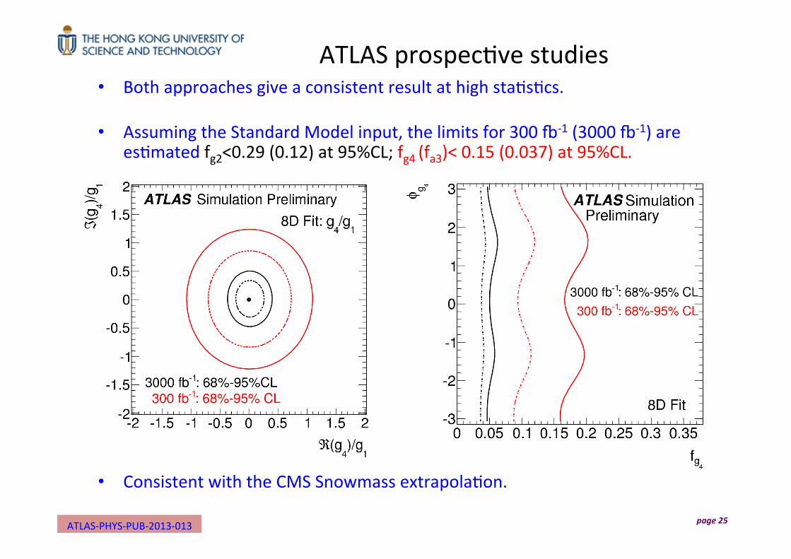
•  Both  approaches  give  a  consistent  result  at  high  sta@s@cs.    

•  Assuming  the  Standard  Model  input,  the  limits  for  300  D-­‐1  (3000  D-­‐1)  are  es@mated  fg2<0.29  (0.12)  at  95%CL;  fg4  (fa3)<  0.15  (0.037)  at  95%CL.                                

•  Consistent  with  the  CMS  Snowmass  extrapola@on.  

ATLAS-­‐PHYS-­‐PUB-­‐2013-­‐013  

Independent  sensi@vity  es@mate  

                         page  26  

                         page  27  

•  Effec@ve  field  theory  descrip@on  valid  up  to  some  new  physics  scale  Λ.    

•  Spin-­‐0    par@cle  interac@on  Lagrangians  with  vector  bosons.  

CERN-­‐2013-­‐004  

Higgs  Characterisa@on  model  

ki  are  dimensioneless  coupling  parameters.  All  couplings  “k”  are  real.    Mixing  between  0+  and  0-­‐  is  introduced  through  cos  α    

The  CP-­‐viola@ng  coupling  ra@o  a3/a1  corresponds  to      

 kAVV/kSM  tgα  ~  

Independent  sensi@vity  es@mates  

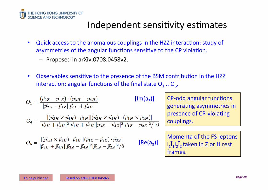
•  Quick  access  to  the  anomalous  couplings  in  the  HZZ  interac@on:  study  of  asymmetries  of  the  angular  func@ons  sensi@ve  to  the  CP  viola@on.  –  Proposed  in  arXiv:0708.0458v2.  

 •  Observables  sensi@ve  to  the  presence  of  the  BSM  contribu@on  in  the  HZZ  

interac@on:  angular  func@ons  of  the  final  state  O1  ..  O6.    

                         page  28  To  be  published   Based  on  arXiv:0708.0458v2  

CP-­‐odd  angular  func@ons  genera@ng  asymmetries  in  presence  of  CP-­‐viola@ng    couplings.  

Momenta  of  the  FS  leptons  l1Ī1l2Ī2  taken  in  Z  or  H  rest  frames.        

[Im(a3)]  

[Re(a3)]  

14  TeV  collisions  

•  MG5  simula@on  of  the  HàZZ*à4l  process  and    dominant  backgrounds.  Pythia  6  parton  shower    and  PGS  detector  simula@on.    

•  Generic  LHC-­‐like  detector.                    

•  Combinatorial  4l  final  state  selec@on.  

 page  29  5O

0.5− 0.4− 0.3− 0.2− 0.1− 0 0.1 0.2 0.3 0.4 0.5ex

pN

0

10

20

30

40

50

ZZ-Continuum) = 1.0αcos() = 0.5αcos(

-1 L = 300 fb∫

4O0.5− 0.4− 0.3− 0.2− 0.1− 0 0.1 0.2 0.3 0.4 0.5

exp

N

0

10

20

30

40

50

60

70

80 ZZ-Continuum) = 1.0αcos() = 0.5αcos(

-1 L = 300 fb∫

1O1− 0.8− 0.6− 0.4− 0.2− 0 0.2 0.4 0.6 0.8 1

exp

N

0

5

10

15

20

25

30

ZZ-Continuum) = 1.0αcos() = 0.5αcos(

-1 L = 300 fb∫

To  be  published  

Asymmetries  •  Propor@onal  to  the  probed  anomalous  couplings.  Becomes  non-­‐zero  only  if  

the  corresponding  BSM  contribu@on  is  present.      •  The  asymmetries  are  defined  through  the  simple  coun@ng  experiment:    

                         page  30  

αcos 0.00 0.05 0.10 0.15 0.20 0.25 0.30 0.35 0.40 0.45 0.50 0.55 0.60 0.65 0.70 0.75 0.80 0.85 0.90 0.95 1.00

| i|A

0

0.02

0.04

0.06

0.08

0.1

0.12

0.141O2O3O4O5O6O

To  be  published  

Asymmetries  amplitudes  for  HàZZ*à4l  process  at  14  TeV  including  background  es@mates.  

HL-­‐LHC  exclusions  •  95%  CL  exclusions  based  on  

asymmetry  significances  are  consistent  with  ATLAS  and  CMS  es@mate.    

•  Full  likelihood  fit  of  all  observables  may  improve  this  result.      

                         page  31  

300  D-­‐1  excluded  at  95%CL  

3000  D-­‐1  excluded  at  95%CL  

To  be  published  

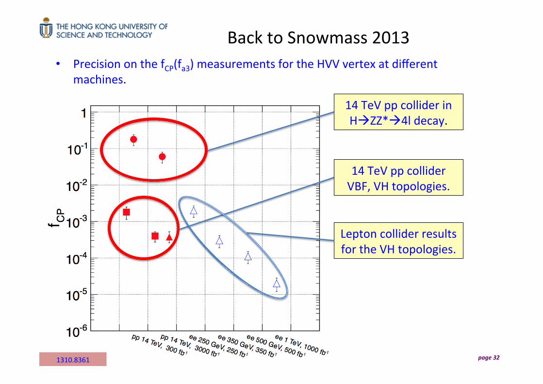
Back  to  Snowmass  2013  •  Precision  on  the  fCP(fa3)  measurements  for  the  HVV  vertex  at  different  

machines.  

                         page  32  

14  TeV  pp  collider  in  HàZZ*à4l  decay.  

14  TeV  pp  collider  VBF,  VH  topologies.    

Lepton  collider  results  for  the  VH  topologies.    

1310.8361  

Back  to  Snowmass  2013  

•  Available  es@mates  show  that  the  HL-­‐LHC  will  achieve  an  order  of  10-­‐2  precision  on  the  fa3  measurements  in  decays.  Can  we  do  beuer?    

                         page  33  1310.8361  

Summary  

•  Fixed  hypotheses  spin  and  parity  results  suggest  we  deal  with  a  spin-­‐0  par@cle.    

•  Current  CP-­‐mixing  and  anomalous  couplings  results  from  CMS  are  consistent  with  the  Standard  Model  expecta@ons.  –  Beuer  limits  than  expected.  –  The  corresponding    ATLAS  measurements  are  in  progress.  

 •  The  exis@ng  projec@ons  all  agree  that  for  the  most  sensi@ve  channel  

HàZZ*à4l,  the  upper  limit  on  fa3  of  the  order  of  10-­‐2  will  be  set  at  3000  D-­‐1.  –  The  WW  decay  will  provide  weaker  exclusion.  –  The  VBF/VH  topologies  provide  stronger  fa3  limit  due  to  the  different  CS  

ra@os.  

•  Hff  vertex  measurements  need  to  be  seriously  explored.  Most  importantly,  the  Hττ.    

                         page  34  

Backup                            page  35  

The  spin-­‐0  par@cle  •  The  absolute  majority  of  these  studies  were  based  on  direct  exclusion  of  

alterna@ve  JP  hypotheses  in  favor  of  the  JP=0+  suggested  by  the  Standard  Model.  

                     •  DØ  constraint  on  0-­‐  scenario  at  97.9%  CL  from  W/Z+bb  (DØ  Note  6406-­‐CONF);  

constraint  on  2+  scenario  at  99.9%  CL  from  W/Z+bb  (DØ  Note  6387-­‐CONF).  –  Assuming  Standard  Model  produc@on  CS  X  BR.  

•  The  only  data-­‐based  CP-­‐mixing  study  to-­‐date  is  published  by  CMS  in  ZZ*à4l  decay    

                         page  36  

JP  hypotheses  ATLAS     CMS  exclusion  

Exclusion  (%CL)   channel   Exclusion  (%CL)   channel  

0-­‐   97.8   ZZ*   >99.9   ZZ*  

1+   >99.9   ZZ*+WW   >99.9   ZZ*+WW  1-­‐   99.7   ZZ*+WW   >99.9   ZZ*+WW  2+m   >99.9   ZZ*+WW+γγ   >99.9   ZZ*+WW+γγ  

Phys.  Le).  B  726  (2013),  pp.  120-­‐144   CMS-­‐PAS-­‐HIG-­‐13-­‐005   CMS-­‐PAS-­‐HIG-­‐13-­‐002  

CMS-­‐PAS-­‐HIG-­‐13-­‐002  

arXiv:1411.3441v1  

Experimental  CP-­‐mixing  studies  •  Spin  and  parity  analyses  to-­‐date  suggest  that  the  observed  Higgs  boson  

has  spin  0.  Dominant  CP-­‐even  parity  (JP=0+)    established  in  ZZ*  decay.    

•  Almost  all  Beyond  the  Standard  Model  theories  with  extended  Higgs  sector  predict  possible  anomalous  contribu@on  and/or  CP-­‐viola@on  in  the  Higgs  sector.    

•   Di-­‐boson  decays  and  VBF  produc@on  probing  the  VVH  vertex.  –  Already  accessible  with  the  run-­‐I    LHC  dataset  (25  D-­‐1).  Some  work  is  

done  in  ZZ*  decays.  –  Growing  interest  to  individual  and  combined  VBF  studies:  VBF  Hàττ,  

Hàγγ,  HàWW  and    ZZ.      

•   Fermion  decays  probing  Hff  vertex.  –  Signal  observed  in  Hàττ.  Most  probably,  run-­‐I  data  will  not  allow  for  

meaningful  measurement,  however,  run-­‐II  sta@s@cs  should  greatly  help.  

–   uH?    

                         page  37  

Recent  CMS  results  (ICHEP  2014)  •  Mixing  in  the  spin-­‐0  sector:  results  in  ZZ*,  WW*  and  combina@on.  

 

                         page  38  

Amplitude  used  for  the  ZZ*  analysis  now  includes  the  Zγ*  and  γγ*  terms.        

In  both  ZZ*  and  WW*  analyses,  an  expansion  of  a1,  reflec@ng  possible  BSM  contribu@on  to  the  tree-­‐level  SM  coupling.        

Expected  couplings  size  in  the  SM:    a1=2,  a2,  a2Zγ,a2γγ~10-­‐3.  CMS  limit  at  20xSM.    The  Zγ*  and  γγ*  terms  in  principle  modify  the  m34  distribu@on.  But  they  are    very  sensi@ve  to  the  m12  cut  (40  GeV  in  CMS).    Are  we  sensi@ve?  Is  γ*γ*  interes@ng  provided  we  measure  Hàγγ?  

Backup                            page  39  

Backup                            page  40  

Prospec@ve  studies  -­‐  II  

                         page  41  

•  ATLAS:  Dedicated  Monte  Carlo    CP-­‐mixing  study  in  HàZZ*à4l  decay  channel  for  14  TeV,  300  D-­‐1  and  3000  D-­‐1.  –  Generator  level  with  smearing  func@on  and  weights  modeling  

detector  resolu@on  and  efficiency.    

•  Measurement  of    (g1,  g4)  and  (g1,  g2)  pairs  in  ra@os.            

The  results  of  the  measurement  is  expressed  in  (fg2,  fg4,  Φg2,  Φg4)  parametriza@on.    In  this  nota@on,  fa3=  fg4.  

Re(g4 )g1

Im(g4 )g1

ATL-­‐PHYS-­‐PUB-­‐2013-­‐013   Arxiv:1208.4018  

                         page  42  

ME-­‐observable  fit  

•  Considering  several  observables  sensi@ve  to  the  rela@ve  magnitude  and  sign  of  the  real  and  complex  parts  of  coupling.    –  Log(|ME(0+)|2/|ME(0-­‐)|2):  |g4|/g1  sensi@ve.  –  Log(|ME(0+)|2/|ME(0+h)|2):  |g2|/g1  sensi@ve.  

 •  Pdfs  are  extended  to  2D  by  a  ZZ-­‐sensi@ve  

discriminant.  –  BDT  trained  per  final  state  on  parity    

insensi@ve  observables:    pT,  η,  m4l,  cosθ*,  Δφ.    

•  Test  sta@s@c:  -­‐2ln(L)                                                                                                                                                                                                                                                                                                                                                                                                                                                  where  Nsig  (fixed  to  expecta@on)  and  Nbckg  are  signal    and  background  expecta@ons  respec@vely  and    μ  is  the  signal  strength.  

 

Parity-­‐sensi@ve  observable  

BDT(J=0    vs  Z

Z)  

ZZ  

Signal  

For  a  given  (g1,g4)  

L(µ,N, syst) = (µ ⋅Nsig ⋅ pdfsig + Nbckg ⋅ pdfbkg )∏

ATLAS  prospec@ve  studies  

                         page  43  

•  Both  approaches  give  a  consistent  result  at  high  sta@s@cs.    

•  Assuming  the  Standard  Model  input,  the  limits  for  300  D-­‐1  (3000  D-­‐1)  are  es@mated  fg2<0.29  (0.12)  at  95%CL;  fg4<  0.15  (0.037)  at  95%CL.  

ATLAS-­‐PHYS-­‐PUB-­‐2013-­‐013  

ATLAS  prospec@ve  studies  

                         page  44  

•  Exclusion  limits  for  |g4|/g1  and  |g2|/g1  at  300  D-­‐1  and  3000  D-­‐1.  

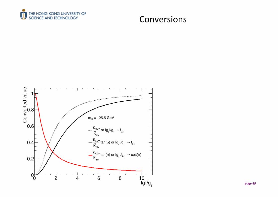
Conversions  

                         page  45  1

|/gi

|g0 2 4 6 8 10

Con

verte

d va

lue

0

0.2

0.4

0.6

0.8

1

= 125.5 GeVHm

g2 f→ 1

|/g2

or |gSMK~

HVVκ∼

g4 f→ 1

|/g4

) or |gα tan(SMK~

AVVκ∼

)α cos(→ 1

|/g4

) or |gα tan(SMK~

AVVκ∼