hierarchical drawing algorithms - brown universityrt/gdhandbook/chapters/hierarchical.pdf ·...

13Hierarchical Drawing Algorithms

Patrick HealyUniversity of Limerick

Nikola S. NikolovUniversity of Limerick

13.1 Introduction . . . . . . . . . . . . . . . . . . . . . . . . . . . . . . . . . . . . . . . . . . . . . . . . . 409Current Approaches and Their Limitations • Overview ofSugiyama’s Framework

13.2 Cycle Removal . . . . . . . . . . . . . . . . . . . . . . . . . . . . . . . . . . . . . . . . . . . . . . 413Heuristics Based on Vertex Orderings • Berger-ShorAlgorithm • Greedy Cycle Removal • Heuristics Based onCycle Breaking • Minimum FAS in a Weighted Digraph •

Other Approaches

13.3 Layer Assignment . . . . . . . . . . . . . . . . . . . . . . . . . . . . . . . . . . . . . . . . . . 417Additional Criteria and Variations of the Problem •

Layer Assignment Algorithms • The Layering AlgorithmsCompared • Layer-Assignment with Long Vertices

13.4 Edge Concentration . . . . . . . . . . . . . . . . . . . . . . . . . . . . . . . . . . . . . . . . 430Intersection Cover • Newbery’s Algorithm

13.5 Vertex Ordering . . . . . . . . . . . . . . . . . . . . . . . . . . . . . . . . . . . . . . . . . . . . 432One-Sided Crossing Minimization • Multi-Layer CrossingMinimization • Planarization – An Alternative

13.6 x-Coordinate Assignment . . . . . . . . . . . . . . . . . . . . . . . . . . . . . . . . . 44113.7 Extensions and Alternatives to Sugiyama’s Framework 443References . . . . . . . . . . . . . . . . . . . . . . . . . . . . . . . . . . . . . . . . . . . . . . . . . . . . . . . . . . 446

13.1 Introduction

In many cases a directed graph represents a hierarchy and we want to draw it in this way.We will define a hierarchy later, but for now it is sufficient to think of a hierarchy as a cycle-free digraph where it is useful for nodes of the graph to be stratified into discrete, parallellayers. Examples of hierarchies or near-hierarchies are, among others, PERT charts forproject management, object-oriented class diagrams, and function call graphs from softwareengineering. As usual, nodes represent entities and edges represent relationships betweenthe entities. Closely related to hierarchically layered drawings and discussed later are radialdrawings where nodes are placed on concentric circles [DDLM04, Bac07] and cyclic leveldrawings, where nodes are placed on “spokes” emanating from a centre-point [BBBF12].

What is common to all of the examples described above is the need to represent allthe relationships graphically so that the positioning of nodes are as consistent with thetransitivity of the relationship as can be achieved. That is, the edges should “flow” in auniform direction. Whether this direction should be top-to-bottom, or left-to-right, dependson the application domain, with different disciplines having different preferences.

Di Battista et al. [DGL+00] conduct an experimental study of directed graph drawingalgorithms. They look at two broad categories of algorithms, those that provide layered

409

410 CHAPTER 13. HIERARCHICAL DRAWING ALGORITHMS

drawings and those that are grid-based. From the point of view of edge crossings, animportant aspect in the readability of graph drawings [PCJ96], the hierarchical or layeredapproach performs better, they conclude.

For digraphs that are almost a hierarchy it still can be possible to take advantage ofthe methods we describe in this chapter. Since the methods work best for hierarchicaldigraphs, however, one may find the results disappointing when applied to a digraph thatis fundamentally non-hierarchical. A method for computing the hierarchical index – thatis, the amount of hierarchy in a directed graph – has been proposed [CHK02].

In addition to the applications we mentioned earlier, it is common and appropriate torepresent computer file systems and social networks as a graph. Due to the possibility ofsymbolic links a graph representation of a computer file system may have directed cycles, andso may be more complicated than a tree. Likewise, a graph representation of relationshipsamong a social network graph may have cycles.

In the following sections we describe the current approaches to drawing directed graphshierarchically and consider in more depth the dominant player, the Sugiyama frameworkfor drawing digraphs. It is perhaps a measure of its effectiveness and its success that themethod has been used to draw undirected graphs, by imposing orientations on the edges.However, as we have mentioned earlier, results may be disappointing if care is not taken inhow orientations of edges are fixed.

13.1.1 Current Approaches and Their Limitations

Force-directed methods, discussed elsewhere in this handbook, can be modified to takeaccount of edge directions, and thus can be used to draw digraphs. Sugiyama andMisue [SM95b] propose modifications of Eades’ spring embedder model [Ead84] to takeaccount of the possible directedness of edges.

Far and away the most popular method of drawing directed graphs is the Sugiyamamethod , or Sugiyama framework [STT81], which separates the nodes into layers. Theidea of layered drawings can be traced back earlier to work by Warfield [War77] andCarpano [Car80]. Systems such as da Vinci [FW95], dot [GKN02] (part of the GraphViz

suite of tools [GN00]), GraphLet [Him00], the AGD graph drawing library [NPT90] and oth-ers implement this framework for drawing directed graphs. In testament to its popularitymany modifications and enhancements have been proposed in the literature. However, theframework has its limitations. Figure 13.1 shows two drawings of C4, firstly drawn usingforce-directed methods and secondly drawn using the Sugiyama framework. In spite of thedirected edge entering node a, by imposing a leveling Figure 13.1b suggests that node d isinferior to the others.

In the following section we describe the Sugiyama framework in general terms. In subse-quent sections we consider the framework in more detail, elaborating on issues specific toeach step of the framework. It should be noted at the outset that this is only a frameworkand for many steps of the process alternative algorithms exist, each with their own merits.Equally important is the fact that the steps may interact with each other and a solution toone step can have a bearing on later steps.

13.1.2 Overview of Sugiyama’s Framework

The Sugiyama framework is motivated by a number of aesthetically desirable propertiesthat make for a more readable graph. Indeed the steps of the Sugiyama framework can beseen to address, in turn, each of the following aesthetics.

13.1. INTRODUCTION 411

a

b

c

d

(a)

a

b

c

d

(b)

Figure 13.1 Two alternative drawings of C4.

• Edges should point in a uniform direction

• Short edges are more readable

• Uniformly distributed nodes avoid clutter

• Edge crossings obstruct comprehension

• Straight edges are more readable

Figure 13.2 demonstrates how these aesthetics are achieved on a typical directed graph1

G. So that all edges are directed uniformly, any directed cycles are broken by reversing asubset of edges (see Figure 13.2b). The resulting graph is then leveled (Figure 13.2c) where,through the introduction of dummy vertices, “long” edges are replaced by a series of shortersegments, after which vertices on each level are permuted in order to reduce edge crossings(Figure 13.2d). Finally, edges spanning more than one level (long edges) are straightenedby adjusting the x-coordinates of their end vertices and by aligning the inserted dummynodes on long edges.

As we have remarked before the Sugiyama framework draws directed graphs as layers ofvertices. We have loosely described a hierarchy in terms of layers of nodes and this is partof its formal definition, also. Definition 13.1 formalizes a level graph, and the definition ofa hierarchy follows from this.

DEFINITION 13.1 A level graph G = (V,E, λ) is a directed acyclic graph with a map-ping λ : V → 1, 2, . . . , k, k ≥ 1, that partitions the vertex set V as V = V1 ∪V2 ∪ · · · ∪Vk,Vj = λ−1(j), Vi ∩ Vj = ∅ for i 6= j, such that λ(v) = λ(u) + 1 for each edge (u, v) ∈ E.

DEFINITION 13.2 A hierarchy is a level graph G(V,E, λ) where for every v ∈ Vj , j > 1,there exists at least one edge (w, v) such that w ∈ Vj−1.

1The figure is due to Bachmaier et al. [BBBF12]; the authors’ permission to reproduce the figure isgratefully acknowledged.


9

10

2

1

43

11

5

6

15

8

714

13

12

(a) Input digraph, G.

9

10

2

1

43

11

5

6

15

8

714

13

12

(b) Cycles removed.

9 10

21

4 3

11

5 6

15

8 7

141312

(c) After leveling.

9 10

21

43

11

5 6

15

87

141312

(d) Edge crossings minimized.

9 10

21

43

11

5 6

15

87

141312

(e) Edges straightened.

Figure 13.2 A digraph drawn according to the Sugiyama framework.

13.2. CYCLE REMOVAL 413

Note that Definition 13.2 restricts all sources of the graph to appear on the first levelbut this may be relaxed if desired. Further, the definition implies that all edges are of unitlength, a property that is necessary for the crossing minimization step. While an inputdigraph may not be a hierarchy initially, the steps described in the following subsectionswill transform it into an equivalent hierarchy.

13.2 Cycle Removal

The first step of the Sugiyama method is a preprocessing step that aims the reversal of thedirection of some edges in order to make the input digraph acyclic. A digraph is acyclic ifit does not contain any directed cycles. Note that the digraph may have undirected cyclesand be acyclic. It is usually assumed that the input digraph has no two-cycles. A two-cycleis a cycle consisting of a pair of edges (u, v) and (v, u). If any are present then one edgeof each pair can be removed before applying the Sugiyama method and reintroduced backinto the final drawing.

The cycle-removal preprocessing step is necessary because the input to the the layer-assignment step must be an acyclic digraph, also called a DAG (directed acyclic graph).Once vertices are assigned to layers, the original direction of the reversed edges can berestored. These are edges which point against the flow in the final drawing. It is alsopossible to remove edges instead of reversing them, and introduce them back after thelayer-assignment step. However, if edges are removed then the layer-assignment step willwork with a subgraph of the input digraph and may have undesirable results.

A set of edges whose removal makes the digraph acyclic is commonly known as a feedbackarc set (FAS). Following the terminology used by Di Battista et al. [DETT99] we call a setof edges whose reversal makes the digraph acyclic a feedback set (FS). Each FS is also aFAS. However, not each FAS is a FS. For example, if a digraph has only one cycle, then theset of all edges in the cycle is a FAS but not a FS.

It is always possible and easy to find a FS for a digraph. Any linear ordering of thevertices partitions the edge set into two subsets, a subset of edges whose source is beforetheir target in the ordering, and a subset of edges edges whose source is after their targetin the ordering. Each of the two subsets is a FS. However, it might be much harder to finda FS with some specific properties.

A typical requirement for a FS is to contain as few edges as possible because they are theedges against the flow in the final drawing. The problem of finding a minimum-cardinalityFS is known as the minimum FS problem. As we mentioned above not every FAS is aFS. However, it is easy to see that every minimal cardinality FAS is also a FS. Thus, theminimum FS problem is as hard as the widely studied minimum FAS problem which isknown to be NP-hard [Kar72, GJ79].

Any heuristic for solving the minimum FAS problem can be applied for solving the min-imum FS problem as well. Consider a digraph G = (V,E) and let F ⊆ E be a FAS. F is aminimal FAS if for each e ∈ F there is a cycle in (E \F )∪e. If F is not minimal then oneby one we can remove edges from it until it becomes minimal. However, such a procedurewill add additional running time.

The remainder of this section summarizes the known heuristics for solving either theminimum FS problem or the minimum FAS problem. Some of the FAS heuristics have beenoriginally proposed as heuristic for solving its complimentary problem, i.e., the maximumacyclic subgraph problem.


13.2.1 Heuristics Based on Vertex Orderings

As we mentioned above any linear ordering of the vertices provides two FSs. Imagine thevertices placed on a horizontal line in accordance with the provided linear ordering. Thefirst FS consists of the edges with direction from left to right, and the second FS consistsof the edges with direction from right to left. It can be shown that there are digraphs andlinear orderings of the vertices for which both FSs have the same size [BS90]. Thus, thesimple approach is a 2-approximation heuristic for solving both the minimum FS and FASproblems.

It is clear that the outcome of this simple approach depends on the linear ordering of thevertices. Some researchers have suggested to use a linear ordering provided by a depth-firsttraversal [RDM+87, GKNV93]. This is based on the intuition that such an ordering maybe “natural” for the digraph i.e., it may look “natural” to the viewer that the edges againstthe flow are drawn this way. A depth-first-traversal ordering can be computed in lineartime. Here it is assumed that always the set of edges with direction to the left, i.e., againstthe ordering, are chosen as FSs. These are the back edges in the depth-first-traversal tree.Their number can be at most |E| − |V | − 1 which could be high for dense digraphs.

Eades et al. proposed two alternative linear orderings [ELS89]. The first one is basedon the intuition that vertices with large outdegree should appear at the top of the finaldrawing. First in the ordering comes vertex v with the maximum d+

G(v), next comes vertexv′ with the maximum d+

G−v(v′), etc. This linear ordering can be computed in linear time

and reportedly gives smaller FSs than the ordering provided by the depth-first search.

The second linear ordering proposed by Eades at al. is the result of a divide-and-conquerapproach. Assuming an input digraph G = (V,E) the vertices of which have to be assignedthe labels i, i+ 1, . . . , i+ |V |− 1, the recursive procedure for assigning these labels works asfollows. If |V | = 1 then the single vertex gets the label i. Otherwise V is partitioned intotwo subsets V1 and V2 and the procedure is applied recursively to G[V1] and G[V2] with setsof labels i, i+ 1, . . . , i+ |V1|− 1 and i+ |V1|, i+ |V1|+ 1, . . . , i+ |V |− 1, respectively. V1 andV2 are such that for each pair of vertices (v1, v2) ∈ V1 × V2 d

+G(v1) ≥ d+

G(v2). If |V | is eventhen V1 and V2 have the same cardinality. Otherwise, V1 contains a singe vertex, and V2

contains the rest of the vertices. It takes O(min((|V |+ |A|)log|V |, |V |2)) time to computethis linear ordering. However, the the authors have observed that it regularly obtains results20% better than the results obtained by their other ordering. They also prove performanceguarantees for dense digraphs.

13.2.2 Berger-Shor Algorithm

The first polynomial-time algorithm for solving the minimum FAS problem with an approx-imation ratio less than 2 in the worst case is the algorithm proposed by Berger and Shor in1990 [BS90].

Consider a digraph G = (V,E) and let Ea ⊂ E denote a set of edges such that G[Ea] isacyclic. Let also δ(v) denote all edges adjacent to vertex v, and δ−(v) and δ+(v) denote thesets of incoming and outgoing edges of v, respectively. The algorithm starts with an emptyset Ea and one by one scans all vertices of G, in an arbitrary order. For each vertex v ∈ Vif d+(v) ≥ d−(v) then Ea ← Ea ∪ δ+(v). Otherwise, Ea ← Ea ∪ δ−(v). After processingvertex v it is deleted from G (together with its adjacent edges).

The time complexity of this algorithm is O(|V | + |E|). Berger and Shor prove thatG′ = (V,Ea) is a DAG and thus F = E\Ea is a FAS. They also propose a modification to thealgorithm for making sure the FAS is minimal. It consists of running a strongly connectedcomponents algorithm before processing each vertex, adding the edges between strongly

13.2. CYCLE REMOVAL 415

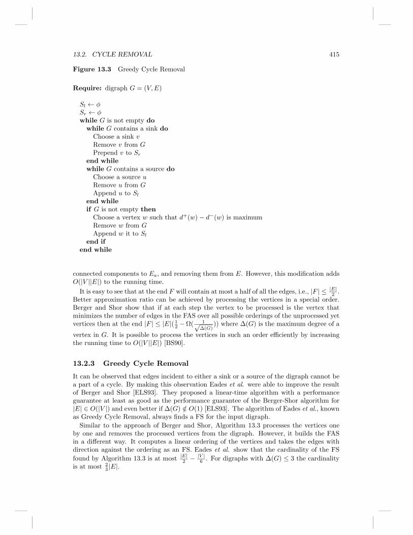
Figure 13.3 Greedy Cycle Removal

Require: digraph G = (V,E)

Sl ← φSr ← φwhile G is not empty do

while G contains a sink doChoose a sink vRemove v from GPrepend v to Sr

end whilewhile G contains a source do

Choose a source uRemove u from GAppend u to Sl

end whileif G is not empty then

Choose a vertex w such that d+(w)− d−(w) is maximumRemove w from GAppend w it to Sl

end ifend while

connected components to Ea, and removing them from E. However, this modification addsO(|V ||E|) to the running time.

It is easy to see that at the end F will contain at most a half of all the edges, i.e., |F | ≤ |E|2 .Better approximation ratio can be achieved by processing the vertices in a special order.Berger and Shor show that if at each step the vertex to be processed is the vertex thatminimizes the number of edges in the FAS over all possible orderings of the unprocessed yetvertices then at the end |F | ≤ |E|( 1

2 −Ω( 1√∆(G)

)) where ∆(G) is the maximum degree of a

vertex in G. It is possible to process the vertices in such an order efficiently by increasingthe running time to O(|V ||E|) [BS90].

13.2.3 Greedy Cycle Removal

It can be observed that edges incident to either a sink or a source of the digraph cannot bea part of a cycle. By making this observation Eades et al. were able to improve the resultof Berger and Shor [ELS93]. They proposed a linear-time algorithm with a performanceguarantee at least as good as the performance guarantee of the Berger-Shor algorithm for|E| ∈ O(|V |) and even better if ∆(G) /∈ O(1) [ELS93]. The algorithm of Eades et al., knownas Greedy Cycle Removal, always finds a FS for the input digraph.

Similar to the approach of Berger and Shor, Algorithm 13.3 processes the vertices oneby one and removes the processed vertices from the digraph. However, it builds the FASin a different way. It computes a linear ordering of the vertices and takes the edges withdirection against the ordering as an FS. Eades et al. show that the cardinality of the FS

found by Algorithm 13.3 is at most |E|2 −|V |6 . For digraphs with ∆(G) ≤ 3 the cardinality

is at most 23 |E|.


Sander has proposed a modification to Algorithm 13.3 similar to the modification whichinvolves the computation of strongly connected components in the Berger-Shor algo-rithm [San96b]. It decreases the running time to O(|V ||E|) but reportedly leads to betterresults in practice. Generalizing the ideas of Sander, Eades and Lin showed how Algo-rithm 13.3 can be modified to guarantee that no more that one quarter of the edges will bereversed for cubic digraphs [EL95].

13.2.4 Heuristics Based on Cycle Breaking

Most of the heuristics discussed above focus on computing linear orderings of the verticeswhich provide FSs. Alternative point of view the minimum FAS problem (and also theminimum FS problem) is to build the FAS edge by edge choosing edges which belong tocycles.

A very simple algorithm based on this approach is the following one. Start with twoempty sets S and T and scan all edges one by one. For each edge e, if S ∪ e is acyclicthen add e to S. Otherwise add e to T . It is easy to show that at the end of this processboth S and T are acyclic and the smaller of the two sets provides a FAS with at most ahalf of all the edges. Note that T is a minimal FAS, while S might not be.

Related to this approach is the heuristic implemented by Gansner et al. in their systemdot [GKNV93]. It takes one non-trivial strongly connected component of the digraph ata time, in an arbitrary order. Within each component it performs a depth-first traversaland adds to the FS an edge which participates in a maximum number of cycles. This isrepeated until there are no more non-trivial strongly connected components. Gansner etal. report that this heuristic performs well in practice. They also observed that it reversesedges whose direction against the flow is “natural” for the input digraph [GKNV93].

13.2.5 Minimum FAS in a Weighted Digraph

In some applications edges are assigned nonnegative weight. Then it might be requiredto reverse not the minimum number of edges but a set of edges with the minimum totalweight. Demetrescu and Finocchi proposed an algorithm for the weighted minimum FASproblem that runs in O(|V ||E|) time. Their approach compromises between two possibleapproaches, i.e., greedily adding light edges to the FAS, and adding edges that belong to alarge number of cycles. The latter is the approach of Gansner et al., which we discussed inSection 13.2.4.

The algorithm of Demetrescu and Finocchi is presented as Algorithm 13.4. Within thewhile-loop heavy edges which belong to a large number of cycles become progressively morelikely to be added to the FAS F . Note also that at the end edges which do not form a cyclewith E \F are excluded from F , thus making sure F is minimal. Demetrescu and Finocchialso prove that their algorithm approximates a minimum FAS of the input digraph G withina ratio bounded by the length of a longest simple cycle of G [DF03].

13.2.6 Other Approaches

There are other approaches to the minimum FAS problem which we would like to refer thereader to. These include the heuristic of Flood [Flo90], and the best-known approximationalgorithm which achieves a performance ratio O(log |V | log log |V |), and requires to solve alinear program [ENRS95, Sey95]. An interesting result is that all minimal solutions can beenumerated with polynomial delay [SS97].

13.3. LAYER ASSIGNMENT 417

Figure 13.4 Algorithm of Demetrescu and Finocchi

Require: digraph G = (V,E), w : E → R

F ← φwhile V,E \ F ) is not acyclic do

Let C be a simple cycle in (V,E \ F )Let (x, y) be a minimum weight edge in CLet ε = w(x, y)for all (u, v) ∈ C dow(u, v)← w(u, v)− εif w(u, v) = 0 thenF ← F ∪ (u, v)

end ifend for

end whilefor all (u, v) ∈ F do

if (V,E \ F ∪ (u, v)) is acyclic thenF ← F \ (u, v)

end ifend for

For an exact ILP approach to the minimum FAS problem we refer the reader to the workof Grotschel et al. and Rienelt et al. [GJR85, Rei85]. Their study of the facial structure ofthe acyclic subgraph polytope can be used for finding the minimum FS by a branch-and-cutalgorithm.

13.3 Layer Assignment

Consider a DAG G = (V,E) with a set of vertices V and a set of edges E. Let L =L0, L1, . . . , Lh be a partition of the vertex set of G into h ≥ 1 subsets such that if(u, v) ∈ E with u ∈ Lj and v ∈ Li then i < j. L is called a layering of G and the sets L0,L1, . . ., Lh are called layers. A DAG with a layering is called a layered DAG. The problemof partitioning the vertex set of a graph into layers is known as the layering problem or thelayer assignment problem.

Sometimes the term levels is used instead of layers. It emphasizes the usual visual rep-resentation of layers as mapped to either parallel horizontal lines or concentric circles. Inthis section we consider the layer assignment problem without relating it to a specific vi-sual representation. The example drawings we give have only illustrative character. Theyemploy the parallel horizontal levels convention, i.e., all vertices in layer Li are placed onthe horizontal level with an y-coordinate equal to i.

Let l(u,L) be the number of the layer that contains vertex u ∈ V , i.e., l(u,L) = i if andonly if u ∈ Li. Sometimes l(u,L) is called rank of vertex u. The span of edge e = (u, v) inlayering L is defined as s(e,L) = l(u,L)− l(v,L). Clearly, s(e,L) ≥ 1 for each e ∈ E; edgeswith a span 1 are tight edges; edges with a span greater than 1 are long edges. A layeringof G is proper if all edges are tight. The layering found by a layering algorithm might notbe proper because only a small fraction of DAGs can be layered properly and also becausea proper layering may not satisfy other layering requirements.


L1

L3

L2

L0

(a) A layered DAG with 4 layers and 5dummy vertices.

L0

L1

L2

L3

L4

(b) A layered DAG with 5 layers and 4dummy vertices.

Figure 13.5 Two alternative layered drawings of the same DAG with introduced dummyvertices which subdivide long edges. Dummy vertices are represented by transparentsquares.

Within the Sugiyama method the vertex ordering algorithms applied after the layer as-signment phase assume that their input is a DAG with a proper layering. Thus, if thelayering found at the layering phase is not proper then it must be transformed into aproper one. Normally, this is done by introducing so-called dummy vertices which subdi-vide long edges (see the illustration in Figure 13.5). Formally, let e = (u, v) be an edge withl(u,L) = j and l(v,L) = i and s(e,L) = j− i > 1. Then we add dummy vertices di+1

e , di+2e ,

. . . , dj−1e to layers Li+1, Li+2, . . . , Lj−1 respectively and we replace edge e by the path

(u, dj−1e , . . . , di+1

e , v). We refer to vertices which are not dummy as original vertices. Wealso denote the set of all dummy vertices introduced to a layered DAG G with a layering Lby D(G,L). Clearly,

|D(G,L)| =∑e∈E

s(e,L)− |E|.

13.3.1 Additional Criteria and Variations of the Problem

If there are no additional requirements it is not hard to find a layering of a DAG. Classicalgraph algorithms such as breadth-first search, depth-first search and algorithms for findinga minimum spanning tree can be easily modified to partition the vertex set of a DAG intolayers. However, normally it is desirable to take into account a number of additional criteriawhen computing a layering [ES90].

It is desirable that |D(G,L)| is as small as possible because a large number of dummyvertices significantly slows down the vertex ordering phase of the Sugiyama method. Thus,one of the goals of a layering assignment algorithm should be to find a layering with asfew as possible dummy vertices. There are also aesthetic reasons for keeping the num-ber of dummy vertices small. A layered DAG with a small number of dummy verticeswould also have a small number of undesirable long edges and edge bends. The problemof finding a layering with the minimum number of dummy vertices is in P. It can be mod-eled as an integer linear programming problem and safely relaxed to a linear programmingproblem for which there are available polynomial-time algorithms. Alternatively, it can beconverted to a min-cost flow or circulation problem, for which there are polynomial-timealgorithms [GKNV93]. Gansner et al. have introduced an integer linear programming (ILP)


model of the problem and a specific network simplex algorithm for solving it which althoughnot proven polynomial-time finds a layering with the minimum number of dummy verticesreportedly fast [GKNV93].

Other parameters of a layering that reflect on the quality of the drawing are the widthand the height of a layering and the edge density between adjacent layers. The height of alayering is the number of layers, and the width is the maximum number of vertices in a layer.Usually these two parameters are used to approximate the dimensions of the final drawing.When measuring the width of a layering the contribution of the dummy vertices may or maynot be taken into account. A more precise definition of the layering width takes into accountboth variable vertex widths and the contribution of the dummy vertices [BLME02, HN02a].The area of a layering, used to approximate the area of the final drawing, is defined as theproduct of the layering width and the layering height.

A layering with the minimum height can be found in linear time by the longest-pathalgorithm [ES90]. It is also easy to find a layering with the minimum number of dummyvertices subject to an upper bound on the number of layers. The ILP model of Gansneret al. can be easily modified to take such an upper bound into account without making itmore difficult to solve.

It is trivial to find a layering with the minimum number of original vertices per layerand no upper bound on the height. Any layering with a single vertex per layer is anoptimal solution. However, it is NP-hard to find a layering with a given upper bound onthe width if the width of the dummy vertices is considered greater than zero [BLME02]. Afew heuristics have emerged since for layering with the minimum width and considerationof dummy vertices [BELM01, TNB04].

It is also NP-hard to find a layering with given upper bounds both on the height andon the width even without taking into account the contribution of the dummy verticesto the width and if all original vertices have the same unit width [ES90]. This variationof the layer assignment problem is equivalent to the precedence-constrained multiprocessorscheduling (PCMS) problem. The Coffman-Graham algorithm, which is an early and highlyinfluential polynomial-time algorithm for solving PCMS approximately, has been also largelyemployed as a layering algorithm [CG72]. Healy and Nikolov have designed a branch-and-cut algorithm which finds layerings with the minimum number of dummy vertices andwith height and width within pre-specified upper bounds [HN02a]. It is not a polynomial-time algorithm but it is an efficient way to find an optimal solution if the problem is notinfeasible. The branch-and-cut algorithm of Healy and Nikolov takes into account variablevertex widths as well as the contribution of the dummy vertices to the width of the layering.

The edge density between layers Li and Lj with i < j is defined as the number of edges(u, v) with u ∈ Lj ∪Lj+1∪ . . .∪Lh and v ∈ L0∪L1∪ . . .∪Li. The edge density of a layeredDAG is the maximum edge density between adjacent layers. Naturally, drawings with lowmaximum and average edge density are clearer and easier to comprehend provided theyare also compact and having not too many long edges. There has not been proposed anyalgorithm which find layerings specifically with consideration of edge density. A few studieshave compared the edge density in layerings found by some of the algorithms mentionedabove [HN02b, NT06, TNB04].

In the next section we take a closer look at the algorithms used for layer assignment.

13.3.2 Layer Assignment Algorithms

The easiest way to partition the vertex set of a DAG into layers is to take any spanningtree of the underlying undirected graph. It can be the depth first search tree or the breadthfirst search tree, for example. For each spanning tree a layering can be generated by picking


a vertex and assigning it to an arbitrary layer, Li. Then assign all its neighbours in thetree to either layer Li−1 or Li+1 depending on the direction of the connecting tree-edge.Then repeat the same with all neighbours of the already assigned vertices and so on untilall vertices are assigned to a layer. It cannot be guaranteed that the set of layers will startwith L1 but this can be easily fixed by shifting the whole set of layers.

In general, this method does not guarantee any properties of the layering. The layerassignment algorithms, which find layerings subject to some of the criteria discussed in theprevious section, broadly fall into two groups. The first group of algorithms are adopted fromthe area of static precedence-constrained multiprocessor scheduling. They produce layeringswith either the minimum height or a specified maximum number of vertices per layer.The second group of algorithms employ network simplex and branch-and-cut techniques,respectively, for minimizing the number of dummy vertices.

List Scheduling Algorithms

The precedence-constrained multiprocessor scheduling problem is the problem ofscheduling n causally related tasks (which represent a parallel program) on m processorswith the goal of minimizing the completion time of the parallel program. This problem isNP-hard when m <∞ [Ulm75]. It is also known as static scheduling because all the taskswith their causal relationship are given in advance and the schedule must be constructedprior executing any of them [KA99]. A simplified version of this problem, when all the taskshave the same computational cost and the communication time between tasks is neglected,is equivalent to the problem of finding a layering of a DAG with at most m vertices per layerand the minimum number of layers. Thus, the earliest static scheduling algorithms whichdeal with simplified models have also found an application as DAG layering algorithms.

Most of the static scheduling algorithms are variations of a generic list scheduling tech-nique which consists of two main steps:

1. Build a scheduling list that contains all the tasks.

2. While the scheduling list is not empty remove the first task from it and scheduleit for execution on a processor which allows earliest start time.

There are two list scheduling algorithms that have been widely employed as layering algo-rithms: the longest-path algorithm and the Coffman-Graham algorithm.

The Longest-Path Algorithm

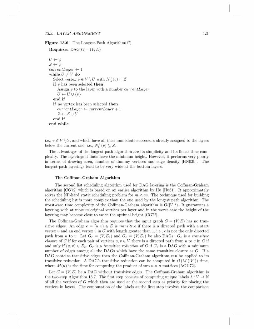
The longest-path algorithm solves the static scheduling problem for m =∞. Let π bethe number of vertices in the longest directed path in a DAG. The longest path algorithmbuilds the scheduling list by assigning priority π to the vertices without outgoing edges. If allimmediate successors of a vertex have been assigned a priority then that vertex is assignedthe lowest of the priorities of its immediate successors minus one. This is repeated until allvertices are assigned a priority. The vertices with the same priority k form layer Lπ−k+1.It has been shown that the longest-path algorithm has linear time complexity. [Meh84].

Algorithm 13.6 is a version of the longest-path algorithm where vertices are assigned tolayers as soon as they are assigned priority. It employs two vertex sets U and Z which areempty in the beginning. The value of the variable current layer is the label of the layercurrently being built. As soon as a vertex gets assigned to a layer it is also added to theset U . Thus, U is the set of all vertices already assigned to a layer. Z is the set of allvertices assigned to a layer below the current layer. A new vertex v to be assigned to thecurrent layer is picked among the vertices which have not been already assigned to a layer,


Figure 13.6 The Longest-Path Algorithm(G)

Requires: DAG G = (V,E)

U ← φZ ← φcurrentLayer ← 1while U 6= V do

Select vertex v ∈ V \ U with N+G (v) ⊆ Z

if v has been selected thenAssign v to the layer with a number currentLayerU ← U ∪ v

end ifif no vertex has been selected thencurrentLayer ← currentLayer + 1Z ← Z ∪ U

end ifend while

i.e., v ∈ V \U , and which have all their immediate successors already assigned to the layersbelow the current one, i.e., N+

G (v) ⊆ Z.

The advantages of the longest path algorithm are its simplicity and its linear time com-plexity. The layerings it finds have the minimum height. However, it performs very poorlyin terms of drawing area, number of dummy vertices and edge density [HN02b]. Thelongest-path layerings tend to be very wide at the bottom layers.

The Coffman-Graham Algorithm

The second list scheduling algorithm used for DAG layering is the Coffman-Grahamalgorithm [CG72] which is based on an earlier algorithm by Hu [Hu61]. It approximatelysolves the NP-hard static scheduling problem for m <∞. The technique used for buildingthe scheduling list is more complex than the one used by the longest path algorithm. Theworst-case time complexity of the Coffman-Graham algorithm is O(|V |2). It guarantees alayering with at most m original vertices per layer and in the worst case the height of thelayering may become close to twice the optimal height [CG72].

The Coffman-Graham algorithm requires that the input graph G = (V,E) has no tran-sitive edges. An edge e = (u, v) ∈ E is transitive if there is a directed path with a startvertex u and an end vertex v in G with length greater than 1, i.e., e is not the only directedpath from u to v. Let Gr = (V,Er) and Gc = (V,Ec) be also DAGs. Gc is a transitiveclosure of G if for each pair of vertices u, v ∈ V there is a directed path from u to v in G ifand only if (u, v) ∈ Ec. Gr is a transitive reduction of G if Gr is a DAG with a minimumnumber of edges among all the DAGs which have the same transitive closure as G. If aDAG contains transitive edges then the Coffman-Graham algorithm can be applied to itstransitive reduction. A DAG’s transitive reduction can be computed in O (M (|V |)) time,where M(n) is the time for computing the product of two n× n matrices [AGU72].

Let G = (V,E) be a DAG without transitive edges. The Coffman-Graham algorithm isthe two-step Algorithm 13.7. The first step consists of computing unique labels λ : V → Nof all the vertices of G which then are used at the second step as priority for placing thevertices in layers. The computation of the labels at the first step involves the comparison


Figure 13.7 The Coffman-Graham Layering Algorithm

Require: A DAG G = (V,E) without transitive edges and an integer W > 0

for all v ∈ V doλ(u)←∞

end forfor i← 1 to |V | do

Choose v ∈ V with λ(v) =∞ such that N−G (v) is minimized;λ(u)← i;

end fork ← 1, L1 ← ∅, U ← ∅while U 6= V do

Choose v ∈ V \ U such that N+G (v) ⊆ U and λ(v) is maximized;

if |Lk| ≤W and N+G (v) ⊆ L1 ∪ L2 ∪ . . . ∪ Lk−1 then

Lk ← Lk ∪ velsek ← k + 1; Lk ← v

end ifU ← U ∪ v

end while

between vertex sets defined as follows. If U1 and U2 are two sets of vertices then U1 < U2

if either

• U1 = ∅ and U2 6= ∅; or

• U1 6= ∅, U2 6= ∅, and maxλ(v) : v ∈ U1 < maxλ(v) : v ∈ U2; or

• U1 6= ∅, U2 6= ∅, maxλ(v) : v ∈ U1 = maxλ(v) : v ∈ U2, and U1 \ v : λ(v) =maxλ(u) : u ∈ U1 < U2 \ v : λ(v) = maxλ(u) : u ∈ U2

In the second step each vertex is assigned to a layer starting from the bottom layer andgoing upward keeping the maximum number of vertices in a layer less than or equal to anupper bound W .

It has been observed that Coffman-Graham layerings have a large amount of dummyvertices and when they are taken into account the area of the layerings can be even worsethan the area of the longest path layerings [HN02b].

Nikolov and Tarassov have proposed a vertex-promotion improvement heuristic which canbe applied after either the longest-path algorithm or the Coffman-Graham algorithm for re-ducing the number of dummy vertices [NT06]. It is a cubic algorithm which is compensatedby its simplicity. We describe the vertex-promotion heuristic in the following section.

Layering with the Minimum Width

It is NP-hard to find a layering with the minimum width if the dummy vertices areassigned non-negative width. This problem can be solved exactly by the Healy and Nikolov’sbranch-and-cut layering algorithm described in Section 13.3.2. In this section we describethe fast heuristic approach proposed by Tarassov et al. [TNB04]. Their min-width layeringalgorithm is the first successful attempt to design a heuristic for layering with the minimumwidth and consideration of dummy vertices. An earlier attempt is the heuristic developedby Branke et al. [BELM01].


Figure 13.8 Min-width(G,W, c)

Requires: DAG G = (V,E), integers W and c

U ← φ; Z ← φcurrentLayer ← 1; widthCurrent← 0; widthUp← 0while U 6= V do

Select vertex v ∈ V \ U with N+G (v) ⊆ Z and ConditionSelect

if v has been selected thenAssign v to the layer with a number currentLayerU ← U ∪ vwidthCurrent← widthCurrent− d+(v) + 1widthUp← widthup+ d−(v)

end ifif no vertex has been selected OR ConditionGoUp thencurrentLayer ← currentLayer + 1Z ← Z ∪ UwidthCurrent← widthUpwidthUp← 0

end ifend while

The min-width algorithm, presented as Algorithm 13.8, is roughly based on the longest-path algorithm which is shown in detail in Algorithm 13.6. Besides the DAG G the min-width algorithm has two input parameters W and c which are explained below.

Similar to the longest-path algorithm, the min-width algorithm builds the layering layerby layer starting from layer 1. The two variables widthCurrent and widthUp are used tostore the width of the current layer and the width of the layers above it, respectively. Thewidth of the current layer, widthCurrent, is calculated as the number of original verticesalready placed in that layer plus the number of potential dummy vertices along edges witha source in V \ U and a target in Z (one dummy vertex per edge). The variable widthUp

provides an estimation of the width of any layer above the current one. It is the numberof potential dummy vertices along edges with a source in V \U and a target in the currentlayer (one dummy vertex per edge).

Vertex v is selected to be placed in a layer subject to an additional conditionConditionSelect which is true if v is the vertex with the maximum out-degree among thecandidates to be placed in the current layer. Such a choice of v results in maximum reduc-tion of widthCurrent. If either no vertex has been selected or ConditionGoUp is true thenthe current layer is completed and the algorithm moves to the next layer. ConditionGoUp

is true if either:

• widthCurrent ≥W and d+(v) < 1, or

• widthUp ≥ c×W .

It is required that d+(v) < 1 when widthCurrent ≥ W because the initial value ofwidthCurrent is determined by the dummy vertices in the current layer and it gets smaller(or at least it does not change) when a vertex with a positive out-degree gets placed in thecurrent layer. In that case, the dummy vertices along edges with a source v are removed fromthe current layer and get replaced by v. If d+(v) ≥ 1, the condition widthCurrent ≥ Won its own is not a reason for moving to the upper layer because there is still a chance to


add vertices to the current layer which will reduce widthCurrent. If d+(v) < 1 then theassignment of v to the current layer increases widthCurrent because it does not replaceany dummy vertices. This is an indication that widthCurrent can not be reduced further.

The min-width layering algorithm has the same time complexity as the longest-pathalgorithm which has been shown to run in linear time [Ulm75]. Through an extensivecomputational study Tarassov et al. have determined that the narrowest layerings arefound for 1 ≤ UBW ≤ 4 and 1 ≤ c ≤ 2. Thus, they propose to run the algorithm forUBW ∈ 1, 2, 3, 4 and c ∈ 1, 2, choose the narrowest of the eight layerings and apply toit vertex-promotion heuristic described in the following section.

Improvement by Promotion of Vertices

The list-scheduling based layering algorithms described above have been shown tofind layerings with a relatively large number of dummy vertices. Nikolov and Tarassovhave proposed a simple vertex-promotion heuristic that can be applied to any layering forreducing its dummy vertex count [NT06].

The vertex-promotion heuristic modifies a given layering L = L0, L1, . . . , Lh of a DAGG by promoting vertices from the layer where they are placed to the layer above. It isapplied only to the original DAG vertices, not to the dummy vertices. To promote vertexv with l(v,L) = k is to move v from Lk to Lk+1 which results in a new partition L∗ =L0, . . . , Lk \v, Lk+1∪v, . . . , Lh. If v ∈ Lh has to be promoted then a new empty layerLh+1 is added to the layering and v is promoted to it. If v has an immediate predecessorplaced in layer Lk+1 then L∗ is not a layering of G. To ensure that the result of thepromotion of vertex v to layer Lk+1 is a layering all immediate predecessors of v in layerLk+1 (if there is any) have to be promoted to layer Lk+2; the same applies to their immediatepredecessors and so on.

The recursive function which performs the described vertex promotion is shown in Algo-rithm 13.9. It takes vertex v as an input parameter and returns dummydiff which is thedifference between the number of dummy vertices before and after the promotion v. In thefor loop, each immediate predecessor u of v which lies in the layer above v gets promoted.The return value of its promotion is added to dummydiff. Then we promote v, subtractfrom dummydiff the number of immediate predecessors of v, and add to it the number ofimmediate successors of v. That is, we promote v one layer up, recursively promoting inadvance all its immediate predecessors which need to be promoted. The time complexityof PromoteVertex is O(|E|) because in the worst case all DAG edges might be traversedwhile promoting vertices recursively.

Then the vertex-promotion heuristic consists of two nested loops shown in Algo-rithm 13.10, an external repeat-until loop and an internal for loop. In the internal loop allvertices in a layered DAG are scanned in no particular order and each vertex with a positivein-degree gets promoted by PromoteVertex (see Algorithm 13.9) if its layering-preservingpromotion reduces the total number of dummy vertices. The external loop goes on untilthe internal loop makes no promotion.

When performed after the min-width layering algorithm, described above, the vertex-promotion heuristic performs only promotions which do not increase the maximum numberof vertices (original plus dummy) in a layer.

There is empirical evidence that 80 iterations of the repeat-until loop are enough forachieving a significant reduction of the number of dummy vertices for graphs with up to100 vertices. If the number of iterations of the repeat-until loop is O(|V |) then the vertex-promotion heuristic is cubic in the worst case.


Figure 13.9 PromoteVertex(v)

Require: A layered DAG G = (V,E) with the layering information stored in a globalvertex array of integers called layering ; a vertex v ∈ V .

dummydiff← 0for all u ∈ N−G (v) do

if layering[u] = layering[v] + 1 thendummydiff← dummydiff+ PromoteVertex(u)

end ifend forlayering[v]← layering[v] + 1dummydiff← dummydiff−N−G (v) +N+

G (v)return dummydiff

Figure 13.10 Vertex-Promotion Heuristic

Require: G = (V,E) is a layered DAG; a valid layering of G is stored in a global vertexarray called layering.

layeringBackUp← layeringrepeatpromotions← 0for all v ∈ V do

if d−(v) > 0 thenif PromoteVertex(v) < 0 thenpromotions← promotions+ 1layeringBackUp← layering

elselayering ← layeringBackUp

end ifend if

end foruntil promotions = 0

Network-Simplex Layering Algorithm

The integer linear programming (ILP) approaches to the layering algorithm have beenintroduced for layering with the minimum number of dummy vertices. The first such ap-proach is the layering technique designed by Gansner, Koutsofios, North and Vo for their sys-tem dot,2 which is probably the most popular system for layered graph drawing [GKNV93].

2http://www.graphviz.org/


Figure 13.11 Network Simplex Layer Assignment

Require: G = (V,E) is a DAG.

feasible tree

while (e =leave edge()) 6= nil dof =enter edge(e)exchange(e, f)

end whilenormalize()balance()

They model the layering problem by the following integer linear program:

min∑

(u,v)∈E

l(u,L)− l(v,L)

subject to: l(u,L)− l(v,L) ≥ 1, ∀(u, v) ∈ El(u,L) ≥ 0, ∀u ∈ Vall l(u,L) are integer

The linear programming relaxation of this integer program always has an integer solutionbecause its constraint matrix is totally unimodular [NW88]. Thus, the integer program canbe solved by the simplex method or any of the polynomial-time algorithms for solving linearprograms. If we add an additional set of constraints of the type l(u,L) ≤ H, where H is anupper bound on the number of layers, the constraint matrix remains totally unimodular.Thus, the problem of finding a layering with the minimum number of dummy verticessubject to an upper bound on the number of layers is also in P.

Gansner et al. go further by introducing a network simplex algorithm for solving their ILPformulation [GKNV93]. It has not been proved to run in polynomial-time but reportedlyrequires a few iterations and runs fast. Its main part is presented in Algorithm 13.11.

The network simplex algorithm is based on the idea that each spanning tree of the under-lying undirected graph of a DAG induces a family of equivalent (in terms of dummy vertexcount) layerings. The algorithm starts with an initial spanning tree which is modified byreplacing edges in order to get a spanning tree that induces a layering with the minimumnumber of dummy vertices. The procedure normalize() at the end of the algorithm is theone that makes sure the set of layers in the induced layering start from L1.

The network simplex starts with an initial spanning tree built by the procedurefeasible tree. Gansner et al. suggest to compute a longest-path layering and then take aspanning tree of short subject to the layering edges. Then each iteration of the while-loopremoves an edge from the spanning tree which breaks the tree into two connected compo-nents. Then a new edge is added to the tree that connects the two components into a newspanning tree. The two edges to leave and enter the tree respectively are chosen so that thenew tree induces a layering with a lower dummy vertex count.

The edge to leave the tree at each iteration of the while-loop is chosen by the functionleave edge() which picks an edge with a negative cut value, or nil if all edges have non-negative cut value. The cut value is defined as follows. If an edge e is removed from thespanning tree, it breaks into two connected components, a tail and a head. The tail is thecomponent that contains the source of e and head is the component that contains its target.The cut value of e is the number of all directed edges from the tail to the head, including e,


(a) Two layers and no dummy vertices. (b) Three layers and fourdummy vertices.

Figure 13.12 Two alternative layerings of the same DAG: a layering with the minimumnumber of dummy vertices may become too wide.

minus the number of all directed edges from the head to the tail. Typically a negative cutvalue of an edge means that the dummy vertex count can be reduced by lengthening thatedge as much as possible, until one of the head-to-tail edges becomes tight. That tight edgeis the one chosen by the function enter edge(). It is the edge with the minimum span inthe layering induced by the spanning tree before removing e.

After the end of the while-loop the spanning tree induces a layering with the minimumnumber of dummy vertices. The procedure balance(), applied at the end, moves verticeswith equal in- and out-degree to a feasible layer with the fewest vertices. This is done inorder to have more even distribution of vertices between layers. Gansner et al. also showhow the network-simplex algorithm can work for graphs with weighted edges and with edgeswhich are required to have span greater than 1 [GKNV93].

In general, layerings with the minimum number of dummy vertices lead to compactdrawings. However some patterns in a DAG can result in too wide layerings with theminimum number of dummy vertices as shown in Figure 13.12.

Healy-Nikolov’s Branch-and-Cut Algorithm

Another ILP approach is the branch-and-cut layering algorithm introduced by Healyand Nikolov [HN02a]. It finds layerings with the minimum number of dummy verticessubject to upper bounds on both the height and the width of the layering if there is anyfeasible solution. Variable vertex width and the contribution of the dummy vertices to thewidth of the layering can be taken into account. Since it solves exactly an NP-hard problem,this algorithm has exponential running time. It is especially designed for producing highquality layerings which satisfy exactly the pre-specified upper bounds on the width and theheight.

Consider a DAG G = (V,E) and let x be the incidence vector of a subset of V ×1, . . . ,H.Healy and Nikolov model the layering problem by the following ILP formulation.

min∑

(u,v)∈E

ρ(u)∑k=ϕ(u)

kxuk −ρ(v)∑

k=ϕ(v)

kxvk

(13.1)


Subject to

ρ(v)∑k=ϕ(v)

xvk = 1 ∀v ∈ V (13.2)

k∑i=ϕ(u)

xui +

ρ(v)∑i=k

xvi ≤ 1 ∀k ∈ LS(u) ∩ LS(v), ∀(u, v) ∈ E (13.3)

∑v∈V ∗

k

wvxvk +Dk ≤W ∀k = 1, . . . ,H (13.4)

∑v∈V ∗

k

xvk ≥ 1 ∀k = 1, . . . , π(G) (13.5)

all xvk are binaries

W and H are upper bounds on the width and height of the layering respectively; π(G)is the number of vertices in the longest directed path in G; ϕ(v) and ρ(v) are respectivelythe lowest and the highest layer where vertex v can be placed in; LS(v) = ϕ(v), . . . , ρ(v)and V ∗k = v ∈ V : ϕ(v) ≤ k ≤ ρ(v). The objective minimizes the sum of edge spans, i.e.,the number of dummy vertices. Equalities (13.2) force each vertex to be placed in exactlyone layer; inequalities (13.3) force each edge to point downward; and inequalities (13.5)introduce the additional requirement of having at least one vertex in the first π(G) layers.This reduces the number of identical layerings (but shifted vertically) if the height of thesolution is less than the upper bound H.

Inequalities (13.4) restrict the width of each layer (including the dummy vertices) to beless than or equal to W : the first term on the left hand side represents the contribution ofthe real vertices to the width of layer Vk while Dk represents the contribution of the dummyvertices. We set

Dk =∑

e=(u,v)∈E

wde

ρ(u)∑l>k

xul −ρ(v)∑l≥k

xvl

where wde is the width of the dummy vertices along edge e. The difference of the two sumsin the parentheses is 1 if edge e = (u, v) spans layer Vk and 0 otherwise.

Healy and Nikolov propose solving their ILP formulation in a branch-and-bound frame-work with the employment of a cutting-plane algorithm at each vertex of the branch-and-bound tree. The cutting-plane algorithm generates valid inequalities for the constraintpolytope of their formulation, some of which are facet-defining. Healy and Nikolov reportthat the running-time of this branch-and-cut algorithm is close to the time necessary forthe ILP solver of CPLEX3 to solve the formulation and they show some examples wherethe branch-and-cut algorithm is significantly faster than CPLEX.

13.3.3 The Layering Algorithms Compared

If any layering is acceptable then probably the easiest way to construct one is either to usethe longest-path algorithm (Section 13.3.2) or to find any spanning tree of the underlyingundirected graph and take the layering induced by it as described in the beginning ofSection 13.3.2. If there is an upper bound on the the number of original vertices perlayer then the Coffman-Graham algorithm, described in Section 13.3.2, is the best solution.

3http://www.ilog.com/products/cplex/


Although the longest-path algorithm finds layerings with the minimum number of layersand the Coffman-Graham algorithm finds layerings with a pre-specified maximum numberof vertices in a layer, their layerings typically lead to drawings which occupy large drawingarea and have too many long edges.

For a compact layering, the network simplex algorithm of Gansner et al., described inSection 13.3.2, is probably the best fast solution. It finds layerings with the minimumnumber of dummy vertices which are also very compact in general. However, there areparticular patterns in graph that may make the network simplex layering either too wide ortoo long. The branch-and-cut algorithm of Healy and Nikolov, outlined in Section 13.3.2,is much slower but in addition to the network simplex algorithm it guarantees that thelayering’s width and height will be within pre-specified bounds. It also considers variablevertex width and the contribution of the dummy vertices to the width of the layering.

The first fast heuristic for layer assignment with the minimum number of vertices per layerwhen both the original and the dummy vertices are considered is the min-width algorithmdescribed in Section 13.3.2. It is not optimal but when followed by the vertex promotionheuristic, described in Section 13.3.2, it finds layerings which on average are narrower thanthe layerings found by any other known layering algorithm. The same vertex-promotionheuristic significantly improves the layerings found by the longest-path and the Coffman-Graham algorithms and makes them comparable to the layerings found by the networksimplex algorithm. The longest-path algorithm followed by the vertex-promotion heuristic isprobably the easiest to implement layering algorithm which results in good-quality layerings.Its only disadvantage is the relatively slow running time, which is cubic in the worst case.

13.3.4 Layer-Assignment with Long Vertices

The layer-assignment algorithms described above assume that all the vertices have similarheight and can be aesthetically arranged on parallel horizontal levels without too muchblank space between the levels. However, in some applications a few vertices in the inputdigraph may have large labels which can make them occupy significantly larger space in thevertical direction than the rest of the vertices. Such long vertices can be allowed to occupymore than one horizontal level in order to achieve aesthetically pleasant drawing.

Misue et al. propose to assign vertices to layers with one of the describe algorithms assum-ing all vertices have the same size. Then in a postprocessing step vertices can be enlargedto their original size and the eventual intersection between vertices are removed [MELS95].However, this approach may lead to drawings which are not aesthetically acceptable.

Recently two studies have proposed layering algorithms that consider the actual sizeof the vertices while assigning them to layers. North and Woodhull have introduced analgorithm that assigns each vertex to two layers which correspond to the lower and theupper bounds of its height, respectively [NW01]. In a subsequent step vertices and edgeswhich cross one or more layers are split into chains of vertices to obtain simpler layering.The second algorithm has been introduced by Friedrich and Schreiber [FS04]. It breaks thelong vertices into chains of vertices while assigning them to layers.

While the special treatment of long vertices makes the final drawing compact, it alsocomplicates the subsequent steps of the Sugiyama method. The vertex-ordering and thecoordinate-assignment steps need to take the long vertices into account. It also becomesmore difficult to rout edges so that they do not go through the long vertices. This mayresult in a large number of edge bends, which is compensated by their short length in thecompact drawing.


13.4 Edge Concentration

Edge concentration is an optional step in the Sugiyama algorithm. It reduces the edgedensity between adjacent layers and the number of edge crossings. It can also reduce thedummy vertex count. The eventual drawbacks are that edge concentration modifies thegraph and may increase the number of layers.

Consider a layered DAG G = (V,E) with a layering L = L1, . . . , Lh. An intersectionin G is a complete bipartite (biclique) subgraph I with a set of source vertices SI and a setof target vertices TI , such that SI ⊆ Lj , and TI ⊆ Li for some i < j. We use the notationI = (SI , TI). If |SI | = |TI | = 1 then the intersection is trivial. The vertex size of I is|S|+ |T |, and the edge size of I is |S| ∗ |T |.

To perform edge concentration on a given nontrivial intersection I is to

• remove all edges between SI and TI from G

• add a new edge-concentration vertex ec to G, i.e., V ← V ∪ ec• add edges e = (ec, u) : u ∈ TI and e = (u, ec) : u ∈ SI to E.

That is, all edges of the intersection C are removed from the graph, a new edge-concentrationvertex is added and all vertices in SI and TI are connected to it by an edge to form a star-like subgraph. An example is shown in Figure 13.13. If SI and TI occupy adjacent layers,i.e., j− i = 1, then a new layer is introduced between Li and Lj and the edge-concentrationvertex ec is placed in it. Otherwise ec is placed in some layer Lk with i < k < j.

Figure 13.13 An example of a bipartite graph before and after the introduction of twoedge-concentration vertices labeled “ec” [New89].

13.4. EDGE CONCENTRATION 431

A set of intersections I = I1, . . . , Ik : 1 ≤ k ≤ |E| is an intersection cover of G if eachedge of G is contained in at least one intersection in the set. The edge concentration stepwithin the Sugiyama method consists of finding an intersection cover I of G and performingedge concentration on each non-trivial intersection in I. If intersections between non-adjacent layers are considered then the dummy vertices are ignored and edge concentrationis applied to intersections of original vertices and edges. After the edge concentration stepdummy vertices are introduced again to subdivide long edges.

In the next section we discuss the different approaches to choosing an intersection coverfor edge concentration.

13.4.1 Intersection Cover

The most important part of the edge concentration step is the choice of an intersectioncover. There are two alternative approaches to this problem proposed in the graph drawingliterature: choose either only intersections between adjacent layers, or only intersectionsbetween non-adjacent layers.

The only edge concentration approach with intersections between non-adjacent layers isthe one employed by AT&T’s dot [GKN02]. Only non-trivial intersections with a singletarget vertex are considered. This is a simple but fast solution for the edge concentrationstep.

Newbery as well as Eppstein et al. suggest a different approach to building the intersec-tion cover [New89, EGM04]. The non-trivial intersections are only intersections betweenadjacent layers and the choice of intersections between two adjacent layers does not dependon the intersections between other layers. Thus, the problem of choosing an intersectioncover of the whole graph is reduced to the problem of choosing a biclique (i.e., completebipartite graph) cover of a bipartite graph.

The best biclique cover from the point of view of edge concentration is the one thatwill result in the fewest number of edges after applying edge concentration. This is whatNewbery calls the Edge Concentration problem and it is defined as a decision problem asfollows.

Edge ConcentrationInstance: A bipartite graph G = (V,E) and a positive number K.Question: Is there an biclique cover I = I1, . . . , Ik : 1 ≤ k ≤ |E| of G with∑ki=1 vs(Ii) ≤ K?

Edge Concentration is NP-complete [Lin00]. Newbery proposes a polynomial-timeheuristic algorithm for solving its optimization version, i.e., to find a biclique coverI = I1, . . . , Ik : 1 ≤ k ≤ |E| with the minimum

∑kj=1 vs(Ij) [New89]. We describe

the heuristic in detail in the following section.

Related to Edge Concentration is the problem of finding a biclique cover of a bipartitegraph with no more than K > 0 bicliques. This problem is known as Complete BipartiteSubgraph Cover, problem GT18 of Garey and Johnson’s NP-complete problems [GJ79].In their paper on confluent layered drawings, Eppstein et al. propose two-layer edge con-centration with a biclique cover which is an approximate solution to the optimization ver-sion of Complete Bipartite Subgraph Cover [EGM04]. Fishburn and Hammer have shownthat Complete Bipartite Subgraph Cover is equivalent to a simply-restricted edge color-ing problem which in turn can be transformed to a vertex coloring problem for bipartitegraphs [FH96]. Thus, Eppstein et al. propose the biclique cover for edge concentrationto be computed by one of the vertex coloring algorithms and specifically by either the


Recursive Largest First (RLF) algorithm of Leighton[Lei79] or the DSATUR algorithm ofBrelaz [Bre79]. Both vertex coloring algorithms have O(|E|3) worst-case time complexityand their solutions can be transformed to a biclique cover in O(|E|2) time.

In the next section we describe in detail Newbery’s heuristic for solving Edge Concentra-tion approximately.

13.4.2 Newbery’s Algorithm

Newbery’s algorithm (Algorithm 13.14) finds an approximate solution to the optimizationversion of Edge Concentration [New89]. Consider a bipartite graph G = (V,E). Two listsof bicliques, B1 and B2, are maintained throughout. B1 is the list of all possible bicliqueswith two source vertices at all times. The bicliques in B1 are sorted in increasing order bynumber of target vertices. Initially B2 contains only the empty biclique, i.e., a biclique withan empty source and target sets. At the end B2 is a list of the non-trivial bicliques for edgeconcentration.

The algorithm takes an input parameter M which is a lower bound on the edge size of abiclique. Newbery defines the edge size of a biclique x as |Sx| ∗ (|Tx| − 1) which is slightlydifferent from the actual number of edges in the biclique. This is chosen in order to avoidbicliques with a single target vertex.

The main part of the heuristic is the for loop that goes through all bicliques in B1 withtwo nested for loops that go through all bicliques in B2. Consider a biclique x ∈ B1 with asource set Sx and a target set Tx. If the edge size of x is less than the lower bound M thenx is discarder from B1. Otherwise x is compared to each biclique y in B2. If x and y havethe same target set then the source vertices of x are added to the source vertices of y. Ifthere is no biclique y in B2 with the same target set as x then x is compared once again toall bicliques in B2 in the second nested for loop. Let Sy and Ty be the source and targetsets of y respectively. Two cases are considered:

• Case 1. If Tx ⊆ Ty then add (Sy ∪ Sx, Tx) to the front of B2 and remove Txfrom the target set of y.

• Case 2. If Ty ⊆ Tx then add (Sx, Tx \ Ty) to the front of B2 and add Sx to thesource set of y, i.e., Sy ← Sy ∪ Sx.

Note that if no other condition becomes true then at the end of the second nested forloop x will be compared to the biclique with the empty target set in B2 which will resultin adding x to B2. At the end all bicliques in B2 with the same target set are merged andbicliques with size less than M are discarded. The biclique with the empty target set willalso be discarded from B2.

The heuristic has O(n4) worst-case time complexity assumed m < n3. The worst case ismuch worse than the typical case encountered in practice.

13.5 Vertex Ordering

For readability edge crossings are one of the crucial parameters of a graph drawing [Pur97].While edge reversal and layer assignment can have an impact on this, it is through the or-dering of vertices that minimizing edge crossings between adjacent layers is mainly achieved(crossings are dependent on the relative order of vertices and not their positions). Thus,this step is often known as the crossing minimization or crossing reduction step.

Crossing minimization is of interest to VLSI-layout researchers and so has a historythat predates much of the graph drawing literature. Garey and Johnson showed that the

13.5. VERTEX ORDERING 433

Figure 13.14 Newbery’s Biclique Cover Heuristic

Require: A bipartite graph G = (V,E) and an integer M > 0

B1 ← φB2 ← φfor all pair of source vertices (u, v) do

add the largest biclique with a source set u, v to B1.end forSort the bicliques in B1 in increasing order by number of target verticesAdd a biclique with empty source and target sets to B2

for all x ∈ B1 doif the Sx ∗ (Tx − 1) < M then

Discard xelse

for all y ∈ B2 doif Tx = Ty thenSy ← Sy ∪ SxContinue the external for loop

end ifend forfor all y ∈ B2 do

if Tx ⊆ Ty thenAdd (Sy ∪ Sx, Tx) to the front of B2

Ty ← Ty \ TxContinue the external for loop

end ifif Ty ⊆ Tx then

Add (Sx, Tx \ Ty) to the front of B2

Sy ← Sy ∪ SxContinue the external for loop

end ifend for

end ifend for


general crossing minimization problem, where permutations for both layers that minimizethe number of crossings are required, is NP -hard [GJ83]; even if one layer is fixed, theproblem still remains NP -hard [EW94]. To counter these apparently negative results,several heuristic and exact methods have been proposed.

While we will mainly be concerned with algorithms that find a drawing with few crossings,the decision version of the problem [GJ83, EW94] also is of interest. In particular, fixed-parameter tractable algorithms have been developed to answer the question of whether anordering of the vertices on one “shore” of a bipartite graph admits a k-crossing (or less)solution when the vertices of the other shore remain fixed [DFH+01a, DW02, DFK03]. Inthe latter an O(1.4656k + kn2)-time decision algorithm is presented.

We may assume that the graph G = (V,E) is properly k-layered. That is, like the levelgraph in Definition 13.1 V = V1 ∪ · · · ∪ Vk, Vi ∩ Vj = ∅, 1 ≤ i 6= j ≤ k, although we donot insist that sources appear on the first layer. The set of edges, E = (u, v)|u ∈ Vi, v ∈Vi+1, 1 ≤ i ≤ k − 1. We let ni = |Vi|,m = |E| and we call N(u) = v ∈ V |(u, v) ∈ E theneighborhood of vertex u. An ordering or permutation, πi, of each Vi provides a solutionfor the crossing minimization problem since it is the relative ordering along the line y = lithat causes edges incident on that layer to cross each other. What we seek, then, is the setof permutations, Π = πi|1 ≤ i ≤ k that minimizes the edge crossings C(G, π1, π2).

In the following sections we will describe the one-layer and two-layer crossing minimizationproblems and solutions. We then go on to discuss techniques for handling multi-layer graphs.Finally, we discuss an alternative to crossing minimization, where the goal is to initiallyextract (and draw) a large planar subgraph, and then draw the remaining edges.

13.5.1 One-Sided Crossing Minimization

Few systems attempt to globally minimize edge crossings. Instead, a heuristic approachbased on one-layer crossing minimization is adopted. This problem, then, is key to many ofthe algorithms that have been proposed for the bi- and multi-partite crossing minimizationproblems. The goal of the one-layered crossing minimization (OLCM) problem is to find,for a given G and π1, the permutation π2 that minimizes C(G, π1, π2).

Counting Crossings

Many of the algorithms we describe below require knowledge of the exact numberof crossings between two layers. Algorithms that compute crossings fall in two categories:those that simply count the crossings and those that can report those edge crossings, also.Since it is possible to have Ω(|E|2) crossings, the latter class of algorithms have runningtime Ω(|E|2) in the worst case. The naive algorithm that considers every pair of edges andruns in O(|E|2) time is, in this sense, optimal.

A further issue is whether the algorithm can be used to compute a crossing numbermatrix which is used by many heuristics. The crossing number matrix, with entries cuv,counts the number of edge crossings between edges incident to u, v ∈ V2, when u is to theleft of v (π2(u) < π2(v)). Since it assumes that the vertices in V1 are fixed, the matrixis only relevant for OLCM. Note that since u is to the left of v or v is to the left of u inany solution then the sum

∑u,v min(cuv, cvu) yields a simple lower bound on the optimal

number of crossings. Junger and Mutzel report that this figure is surprisingly tight on avariety of graphs [JM97]. For dense graphs, Nagamochi [Nag05] presents an upper boundon OLCM of 1.2964 + 12/(δ − 4), where δ > 4 is the minimum degree of a vertex.

Computing the crossing number matrix can be done naively in O(|E|2)-time althoughSander [San94] proposes a sweep algorithm that can compute all entries in O(|V1|+ |V2|+


|E| + C), where C is the number of crossings. Barth et al. [BJM02] investigate a num-ber of different existing algorithms for computing the bilayer crossing number, as well asproposing a new O(|E| log |Vs|)-time algorithm, where Vs is the smaller of the two sets V1

and V2. The algorithm is based on Waddle and Malhotra’s accumulation tree used in theirearlier algorithm [WM99]. Nagamochi and Yamada [NY04] have proposed two algorithmsbased on dynamic programming and divide-and-conquer that run in time O(|V1||V2|) andO(min|V1||V2|, |E| log |Vs|), respectively; both algorithms use O(|E|)-space. For densegraphs these algorithms will outperform the O(|E| log |Vs|)-time algorithm by Barth et al.While Sander’s algorithm turns out to be uncompetitive for large graphs, it does have theadvantage of being able to compute the crossing matrix, which is not possible with eitherof the other faster-running algorithms.

Heuristic Approaches

Eades and Kelly [EK86] propose three heuristics: 1) greedy insertion, 2) greedy switch-ing, and 3) split for the problem. All three methods require the precomputation of thecrossing number matrix.

The greedy insertion heuristic orders vertices left to right on the “free” layer accordingto the one which minimizes the number of crossings that the edges incident to u makewith the edges incident to vertices to u’s right. That is, u is chosen to minimize

∑v∈R,

where R is the set of unchosen vertices. The algorithm runs in time O(|V2|2). The greedyswitching heuristic compares adjacent vertices and switches them if the change in crossingcount, cuv− cvu > 0, where vertex u immediately precedes v. With a precomputed crossingnumber matrix the algorithm’s running time is obviously O(|V2|2). Like greedy switching,the split heuristic is reminiscent of sorting. Here, however, the analogy is with quicksortwhere a vertex, p, is chosen as a “pivot” and the vertices are rearranged into two consecutivesets, Vl and Vr so that cup < cpu for all vertices in Vl and cpu ≤ cup for all vertices in Vr;the left and right subsets of vertices are then ordered recursively. As with quicksort itsworst-case running time is O(|V2|2), but its expected running time is O(|V2| log |V2|).

Eades and Wormald [EW94] propose the median heuristic that assigns to each vertexv ∈ V2 the median position of the x-coordinates of its neighbours, N(v) ⊆ V1. This heuristichas the important property that it will find an ordering with 0 crossings if such an orderingexists; in general, it guarantees an ordering, π2, such that C(G, π1, π2) ≤ 3Copt(G, π1, π2).

Computing the median position for a vertex v has time complexity O(|N(v)|) and, thus,all medians can be found in O(|E|)-time. Sorting the set V2 according to the computedmedians provides the ordering and requires O(|V2| log |V2|)-time.

An alternative to placing a vertex at the median of its neighbours’ x-coordinates is toplace it at the average of them. This gives rise to the barycenter or averaging heuristic[STT81]. It has the same running time bounds as the median heuristic and it, too, willfind a crossing-free ordering if one exists, but there does not exist a general performanceguarantee as exists for the median heuristic.

Some other heuristics of note are Catarci’s [Cat95] assignment heuristic which is basedon an approximation of the linear assignment problem. Catarci claims that the heuristic ismore accurate than the median heuristic, especially when applied to dense graphs. Dresbach[Dre94] has proposed a stochastic heuristic which, having calculated assessment numbersfor each vertex and position (the assessment number is a term borrowed from statistics),begins placing vertices in the position with the smallest assessment position, updating theremaining numbers after each placement.

Genetic algorithms have also been employed as heuristic solutions to the one-layer crossingminimization problem. Makinen and Sieranta [MS94] encode a permutation of V2 as a


tuple. The mutation operator is defined as removing and re-inserting a random memberxi of the tuple to a new random position, with intervening members shifted accordingly.The crossover operation on tuples generates two points i < j, fixes the elements in thetwo tuples between i and j, and reorders the remainders of the two tuples so that they areboth valid permutations. Branke et al. [UBSE98] also use a genetic algorithm for crossingminimization. Due to its more general setting, however, we will postpone its discussionuntil Section 13.7.

Exact Methods

Junger and Mutzel [JM97] present a branch-and-cut algorithm for OLCM that drawson solving the linear ordering problem. Letting δkij be a 0-1 variable that represents theordering of vertices i and j on level k = 1, 2, they develop an expression for the number ofcrossings of a pair of permutations, πi, which will be the objective function to minimize.That is, let δkij = 1 if πk(i) < πk(j) and 0 otherwise; it is clear that δij = 1− δji. Then

C(π1, π2) =

n2−1∑i=1

n2∑j=i+1

∑k∈N(i)

∑l∈N(j)

δ1klδ

2ji + δ1

lkδ2ij (13.6)

For OLCM we assume a fixed π1 and seek the ordering of V2, π2, that minimizes thecrossings. That is, we wish to minimize

C(π2) =

n2−1∑i=1

n2∑j=i+1

∑k∈N(i)

∑l∈N(j)

δ1klδ

2ji + δ1

lkδ2ij (13.7)

As currently posed C(π2) is problematical since it involves quadratic terms. However,using the crossing number for a pair of vertices i and j in V2 from before

cij =∑

k∈N(i)

∑k∈N(i)

δ1lk

we can rewrite equation (13.7) as

C(π2) =

n2−1∑i=1

n2∑j=i+1

cji(1− δ2ji) + cijδ

2ij (13.8)

n2−1∑i=1

n2∑j=i+1

(cij − cji)δ2ij +

n2−1∑i=1

n2∑j=i+1

cji (13.9)

The problem then reduces to finding the vector δ2 ∈ 0, 1(n22 ) that orders the vertices.

In order for the vertices to be given a consistent ordering, we need to impose a “3-cycle”constraint that says that if vertex i precedes vertex j and vertex j precedes vertex k thenvertex i must precede vertex k.

Since cij and cji can be determined beforehand and since the second double sum ofequation (13.9) is a constant, the problem can be written as the following linear program,where δ2

ij is replaced by the more usual xij


minimize

n2∑i=1

n2∑j=i+1

aijxij (13.10)

0 ≤ xij + xjk − xik ≤ 1 1 ≤ i < j < k ≤ n2 (13.11)

0 ≤ xij ≤ 1 1 ≤ i < j ≤ n2 (13.12)

xij an integer (13.13)

This is a well-known formulation of the linear ordering problem and from it the numberof crossings can easily be computed. As the integrality constraint (equation (13.13)) causessignificant difficulty from a computational complexity consideration, a standard approach isto solve a relaxation of the formulation. This approach, called branch-and-cut , is achievedby dropping initially the integrality constraint and as many of the constraints as is necessary,and introducing them subsequently on an as-needed basis. In this case since there are 2

(n2

3

)3-cycle constraints (equation (13.11)) and 2

(n2

2

)hypercube constraints (equation (13.12))

it has been found to be reasonable to begin simply with the hypercube constraints andto introduce constraints for violated 3-cycles until a solution is found. If the solution isnon-integral a branch step takes place where a non-integral variable is selected and twosubproblems are solved, one using 0 as the value of the selected variable and the secondusing 1 as its value.

Algorithm Performance

The most comprehensive experimental analysis of the performance of the various ap-proaches to OLCM that we have discussed is Junger and Mutzel’s [JM97]. Their focus isin bipartite graphs and they consider the OLCM and TLCM versions of the problem usingmost of the heuristics we have discussed above, and others. In this section we will focus ontheir findings for OLCM.

Two classes of experiments are performed. First, the algorithms are applied to randominstances of graphs, of varying edge density, each with 20 vertices on each side. Secondly,motivated by the sparseness that is often observable in graphs of interest, a set of sparsegraphs of varying sizes were considered. It is worth noting that as graphs get denser andthe exact crossing count increases all algorithms perform relatively better. Thus, the secondclass of experiments may tell more about the algorithms’ behaviors.

For the first set of experiments it was observed that the greedy switch, greedy insertionand split heuristics had significantly higher running times as the edge densities increased.This is most certainly due to the requirement to compute the crossing number matrix. Therunning time of the exact method was surprisingly competitive here, although its expo-nential behavior became more obvious on the second class of graphs. The split algorithmperformed best in terms of solution quality and also fared very well in the second class ofsparse graphs.

Over both classes of graphs it would appear that barycenter is the best performer. Itsrunning time is always among the best and its solution quality on the sparse graphs isalways with 3% of optimality. In spite of their similarity, the median algorithm performspoorer than barycenter on both classes of graphs. (The barycenter algorithm is also aneasier algorithm to implement.)

Finally, Makinen and Sieranta [MS94] claim that their genetic algorithm outperforms thebarycenter method in terms of accuracy, although running time is significantly higher.


13.5.2 Multi-Layer Crossing Minimization

In the multi-layer crossing minimization problem (MLCM) we are given a k-layered graph,G = (V1, . . . , Vk, E), with the goal of finding permutations π1, . . . , πk such that the edgecrossings are minimized. Again, both exact and heuristic methods have been proposed.

Before we deal with the full k-layer problem, it is worth considering a number of ap-proaches to the two-layer crossing minimization problem (TLCM). Recall that it was onthis problem that first complexity results were found [GJ83].

Two-Layer Crossing Minimization

For TLCM Valls et al. [VML96] propose a branch-and-bound algorithm that, theyclaim, considers a small fraction of the total search space. They report that the average timetaken to compute Copt for a bipartite graph G(U, V,E), |U | = |V | = 13 and edge-density0.3 was 40 minutes. As the following method appears to give better results we focus on thismethod.

In the course of considering OLCM Junger and Mutzel [JM97] observed that a simplelower bound on the number of crossings proved to be tight. Based on this they developeda branch-and-bound algorithm for TLCM. Given an hour of computation time on a SunSparcstation 10 it was possible to solve to optimality problems varying in size from vertexsize V1 = V2 = 11 with 80% edge density, to vertex size V1 = V2 = 16 with 10% edgedensity. Of heuristic methods for TLCM iterated barycenter was the clear champion, evensurpassing, surprisingly, an iterated scheme based around an exact OLCM algorithm.

Newton et al. [NSV02] consider two new heuristics that, they claim, outperforms theiterated barycenter method. The first method is based on a connection between the bipartitecrossing number and the linear arrangement problem which seeks to order the vertices ofa graph so that the absolute distance between edges is minimized [SSSV01]. Any heuristicsolution to the linear arrangement problem can then be immediately used as a solutionto the bipartite crossing number problem. Two methods based on computing the Fiedlereigenvector of the Laplacian of G are proposed. Another method proposed by the authors[NSV02] that also yields very good results is to repeatedly randomly choose a pair of verticeson the same side, swap their positions and keep this new solution (only) if an improvementresulted.

Heuristic Approaches

The most usual heuristic approach is to repeatedly apply a layer-by-layer sweep of aone-layer crossing minimization algorithm until no further improvement is possible [STT81].That is, for a layer i, the vertices of layers i−1 and i+1 are held fixed if the layers exist and Viis permuted. This procedure is then applied for successively increasing and decreasing i untilthere is no further improvement. Obviously other stopping criteria may be used instead andmore sophisticated control mechanisms can replace the simple up-down strategy describedhere [GKNV93, San95].

An alternative to the layer-by-layer sweep approach was proposed by Matuszewski etal. [MSM99]. The idea, which can also be applied to OLCM, orders all vertices in V =V1 ∪ · · · ∪Vk according to their degree and finds the best position for it on its layer. It doesthis by sifting the vertex through all possible positions (all others remaining fixed), usingthe crossing number matrix to count the crossings that would result at each position.

A different heuristic alternative solves an exact crossing minimization problem on a subsetor window of the multi-layer graph that matches certain criteria [EGDB02]. Some improve-ments over the champion iterated barycenter are presented, although running time remainsa problem with the procedure.


Exact Methods

Following from their work on the linear ordering and OLCM problems Junger etal. derived an integer linear programming (ILP) formulation for MLCM [JLMO97]. Asin the one-layer case, quadratic terms analogous to those appearing in equation (13.7)prevent formulation as a linear program. In this case, however, neither layer is fixed soa different strategy is called for. The proposed solution is to introduce crossing variables,cijkl, denoting whether the edges (i, j) and (k, l) cross when i < j, k < l, i < k and j 6= l.Using this notation along with boolean variables xij to denote π1(i) < π1(j) and yij todenote π2(i) < π2(j) TLCM can be formulated as

minimize∑

(i,j),(k,l)∈E

cijkl (13.14)

− cijkl ≤ yjl − xik ≤ cijkl (i, j), (k, l) ∈ E, j < l (13.15)

1− cijkl ≤ ylj + xik ≤ 1 + cijkl (i, j), (k, l) ∈ E, l > j (13.16)

0 ≤ xij + xjk − xik ≤ 1 1 ≤ i < j < k ≤ n1 (13.17)

0 ≤ yij + yjk − yik ≤ 1 1 ≤ i < j < k ≤ n2 (13.18)

xij , yij , cijkl ∈ 0, 1 (13.19)

If cijkl = 0 then equation (13.15) forces the ordering of vertices i and k to be the sameas that of j and l; similarly, if edges (i, j) and (k, l) cross then yjl − xik = −1, 1, forcingcijkl = 0. Since the variable yjl, l < j does not exist equation (13.16) uses the identityyjl = 1− yjl analogously.

The k-layer problem can then be formulated as

minimize

p−1∑r=1

∑(i,j),(k,l)∈Er

crijkl (13.20)

− crijkl ≤ xr+1jl − x

rik ≤ crijkl (i, j), (k, l) ∈ Er, j < l (13.21)

1− crijkl ≤ xr+1lj + xrik ≤ 1 + crijkl (i, j), (k, l) ∈ Er, l > j (13.22)

0 ≤ xrij + xrjk − xrik ≤ 1 1 ≤ i < j < k ≤ nr (13.23)

xrij , crijkl ∈ 0, 1 (13.24)

whereEr = (u, v) ∈ E|u ∈ Vr, v ∈ Vr+1. (13.25)

Junger et al. [JLMO97] analyze the polytope associated with this ILP formulation andpresent some results that describe facets of the polytope. Healy and Kuusik analyze thecycle space of an MLCM instance [HK04] and derive additional constraints for the ILPformulation (13.20)–(13.24). In his PhD thesis Kuusik [Kuu00] uses these new inequalities.Also described is how additional constraints such as different paths that may not cross, ora group of vertices must appear consecutively can be included.

Algorithm Performance

Matuszewski et al. [MSM99] claim that their global sifting method leads to a 20%improvement over iterated barycenter, although the time taken is considerable. An improvedversion of the algorithm [GSBM01] improves the running time of the original by a factor of10, the authors claim.


Junger et al. [JLMO97] present some preliminary results of their ILP formulation ofMLCM on 3-layer problems. The largest problem has V1 = 26, V2 = 18, V3 = 17, E1 =29, E2 = 29 and takes 330 seconds to find an optimal solution. Kuusik [Kuu00] presentssolutions to larger problems, one measuring over 90 vertices and 112 edges spread over9 levels (Forrester’s “World Dynamics” [GKNV93]). What emerges is that the model issensitive to the number of linear ordering variables, which is driven by the average nodecount per layer.

More recently, semidefinite programming (SDP) methods have begun to offer the prospectof solving larger problems to optimality. Following on from the 2-level case formulated byBuchheim et al. [BWZ10] general k-level solutions have been obtained. Chimani et al.[CHJM11] report on experiments where the method outperformed an ILP implementation.Test cases with up to 20 levels and up to 25 vertices per layer were randomly generatedand while an ILP implementation was capable of solving sparse instances (inter-layer edgedensity, d, of up to 0.1) it was unable to solve a single case where d ≥ 0.2, instances whichtheir SDP solver was routinely able to solve.

13.5.3 Planarization – An Alternative

Mutzel [Mut01] observes that the understandability of a graph may be subtler than simplycounting the number of crossings in the graph. It may be that if a few edges accountfor the crossings then the eye may more easily filter these crossings even if more than theminimum. Thus, an alternative to minimizing edge crossings in a k-level graph presentsitself: determine the maximum level planar subgraph; draw this k-level subgraph withoutcrossings; and, finally, reinsert the “nonplanar” edges, in the expectation that not manycrossings will result. This problem has become of interest in the graph drawing communityand a number of complexity results are known [DFH+01a, DFH+01b].

Mutzel and Weiskircher [MW98] adopt this approach by finding the maximum planarsubgraph, which they call the two-layer planarization problem. They formulate the pla-narization problem as an ILP and they identify a set of facets of the associated polytope inthe cases where one or both layers are fixed. In order to solve k-layer problems they solvea succession of two-layer problems, although this is clearly a sub-optimal strategy.

Kuusik uses ILP methods also for the general k-level planarization problem [Kuu00]. Westate the problem as, given a k-level graph, G = (V,E), find a k-level planar subgraphGp = (V,Ep) so that |Ep| is maximum. An important aspect of finding the maximumk-level planar subgraph is identifying k-level subgraphs that are minimally non-planar andbased on this characterization [HKL04] and the cycle space of the graph [HK04] facets of theassociated polytope are identified. Some of these facets are put to use in a branch-and-cutalgorithm.

An ILP formulation follows easily from that described for the minimum-crossing ILP(13.20)–(13.24). By introducing a binary variable pij for each edge where pij = 1 if andonly if (i, j) ∈ Ep and observing that if (i, j) ∈ Ep and (k, l) ∈ Ep then cijkl = 0, thefollowing constraint expresses the relationship between the two

pij + pkl + cijkl ≤ 2 (13.26)

A complete ILP may then be expressed as

maximize∑

(i,j)∈E

pij (13.27)

13.6. X-COORDINATE ASSIGNMENT 441

subject to

pij + pkl + cijkl ≤ 2 (13.28)

constraints(13.21)− (13.24) (13.29)

pij ∈ 0, 1 (13.30)

Among several equal in size maximum level planar subgraph solutions it may be desirableto favor ones with that will result in fewer crossings. Objective function (13.27) can bemodified to take account of crossing variables and favor solutions with fewer crossings

maximize∑

(i,j)∈E

pij +1

kc + 1

∑(i,j),(k,l)∈E

cijkl (13.31)

where kc is the number of crossing variables.Kuusik reports [Kuu00] being able to solve a set of randomly generated problems of size

k = 8, V1 = · · · = V8 = 12, E = 110 in times ranging from 62(s) to, in an extreme case,343(s).

13.6 x-Coordinate Assignment

Having determined a relative ordering of the vertices on each level the final step requirespositioning the vertices so that, insofar as is possible, the edges are straight and vertices arecentered among their neighbors. Aesthetically straight edges are desirable and this can beachieved by adjusting the positioning – the x-coordinate – of each vertex; there is also someevidence that, perceptually, straight edges are preferable [HEH09]. However, it is likely thatthe width of the graph will increase during this step.

It will be remembered that long edges of the input graph will have been subdivided by theintroduction of dummy nodes and a vertical “flow through” for these vertices is particularlydesirable. Given an edge from level i to level j in the input graph it becomes the path(vi, vi+1, . . . , vj) after the insertion of dummy nodes. It is reasonable to expect that thesub-path (vi+1, . . . , vj−1) be drawn strictly vertical with the (at most two) bends occurringat vertices vi+1 and vj−1, if necessary. Most algorithms in the literature make this a priority.

In their original paper Sugiyama et al. [STT81] propose a mathematical programmingsolution with a quadratic objective function that is a convex combination of two separategoals. Closeness to connected vertices and a balance, or centering, between a vertex’spredecessor neighbors and its successor neighbors are the two criteria identified. Since thesegoals will counteract each other in general they are each weighted by parameters c and 1−c,0 < c ≤ 1 respectively. All dummy nodes associated with a long edge are restricted to bevertically aligned; this presupposes that if two long edges cross, the crossing occurs on eitherthe first or last segment of both edges. Because quadratic programming was computationallyexpensive at the time the authors also proposed a “Priority Layout Method” that operatesin a similar spirit to their crossing-minimization level-by-level sweep. Dummy nodes areassigned a high priority so that they will be aligned, though care is required to ensure thatthe level’s vertex ordering is maintained.

Gansner et al., too, propose exact and heuristic algorithms [GKNV93]. Their exactalgorithm is linear programming-based again. Whereas the quadratic objective function ofSugiyama [STT81] minimizes terms (among others) such as

∑(u,v∈E(x(u)−x(v)2, Gansner

et al. replace the quadratic term by |x(u) − x(v)|. This can now be linearized but at theexpense of introducing an additional variable and two additional constraints for each edge.


1 2

3

4 5

6 7

8 9

10 11 12

13 14 15 16

17 18 19 20

21 22

23

(a) leftmost upper

1 2

3

4 5

6 7

8 9

10 11 12

13 14 15 16

17 18 19 20

21 22

23

(b) rightmost upper

1 2

3

4 5

6 7

8 9

10 11 12

13 14 15 16

17 18 19 20

21 22

23

(c) leftmost lower

1 2

3

4 5

6 7

8 9

10 11 12

13 14 15 16

17 18 19 20

21 22

23

(d) rightmost lower

Figure 13.15 Four “extreme” alignments computed by the Brandes-Kopf algorithm.

Thus, on the grounds that the constraint matrix grows from size V E to size (V +E)E, theydismiss this and propose a heuristic that operates, again, by sweeping up and down over thelevels. Other heuristics have been proposed by Eades et al. who place nodes belonging to anylayer other than the top or bottom according to a degree-weighted barycenter and sweep upand down the levels “until x converges” [ELT96], and Sander with his Pendulum heuristic,which lays out edges Manhattan style and thus may require four bends per edge [San96a].

We close this section with a more detailed look at Brandes and Kopf’s algorithm [BK02],which is considered to be the algorithm of choice for assignment of x-coordinate; the algo-rithm’s running time is linear in the number of vertices and edge segments. As we haveremarked, the algorithm guarantees that, for long edges, at most two bends will occur, andif they are necessary they will occur on the external segments of an edge. Thus, providedthe crossing reduction step has ensured that no two long edges cross internally, all dummy(internal) nodes of a long edge will be aligned.

Similar to Gansner et al. above, the algorithm uses |x(u)− x(v)| as a surrogate for edge-

length. Since, for a set X = xi of real numbers,∑ki=1 |x− xi| is minimized when x is the

median of the set, the algorithm focuses on placing a vertex at the median of its neighbors.

The algorithm firstly computes four “extreme” layouts where each vertex is aligned eitherwith its upper or lower median neighbor and, for each case, vertices on a level are consideredin a left-to-right (left alignment) or right-to-left (right alignment) order. Figure 13.15(reproduced with the authors’ kind permission from their paper [BK02]) illustrates thefour layouts for a given graph. Conflicts – called type 0 conflicts – can arise due to apair of external segments that either cross or are incident upon the same vertex and theseare resolved by the order of consideration. Because the algorithm favors vertical innersegments a crossing of an inner segment with an outer segment – a type 1 conflict – shouldgive precedence to aligning the vertices of the inner segment. A preprocessing step markssuch external segments as being excluded from consideration for alignment.

After each of the four extreme layouts are computed, the layout’s blocks are computed.A block is a maximal set of vertically aligned vertices. These blocks may then be compacted,subject to minimum separation requirements, giving an x-coordinate for each vertex.

Having performed this procedure four times, each with a directional bias, what is sur-prising, perhaps, is that the four candidate positions can be combined so straightforwardlyto get the final position with such satisfactory results. Of the four possibilities the al-gorithm chooses what is called the average median, which, for x1 ≤ x2 ≤ . . . ≤ xk, is

13.7. EXTENSIONS AND ALTERNATIVES TO SUGIYAMA’S FRAMEWORK 443

(xb(k+1)/2c + xd(k+1)/2e)/2. One of the arguments for this choice as opposed to the mean,say, is if a vertex is aligned twice with its upper median neighbor and unevenly positionedin the other two runs the average median will maintain verticality of the segment.

The main body of the algorithm is the four linear sweeps over the segments. The authorsdemonstrate how the type 1 conflicts can be detected in linear time, also. Finally, for eachvertex, the average median of four can be determined in linear time.

13.7 Extensions and Alternatives to Sugiyama’s Framework

There are a few attempts to extend the Sugiyama method beyond the originally proposedframework. Some extensions such as the cycle-removal step and the edge-concentration stephave become standard features of the Sugiyama framework nowadays.

Do Nascimento and Eades have proposed and extensively studied methods for applyinguser constraints to hierarchical drawings interactively [dNE01a, dNE01b]. In particular,they allow the user to interact with an already-computed hierarchical drawing and introduceadditional constraints on the relative position of some vertices. Taking the user constraintsinto account they show how to reapply the Sugiyama method locally to a subgraph of thedigraph and efficiently recompute the coordinates of the affected nodes only. They alsopropose an interactive genetic algorithm with similar features [dNE02].

Although the Sugiyama method has been the most popular method for hierarchicaldrawing of digraphs, several researchers have proposed successful alternative methods.Sugiyama and Misue proposed a magnetic-field method for hierarchical drawing of acyclicdigraphs [SM95a]. A global magnetic field is applied to the edges and they are alignedto it. As a result all edges point unidirectionally without specifically placing the verticeson parallel horizontal lines. Note that in any drawing with edges pointing into the samedirection and continuous y-coordinates of the vertices levels can be easily induced from bya simple quantization procedure.

Utech et al. [UBSE98] proposed a genetic algorithm as an alternative to the Sugiyamamethod. The chromosome contains values which represent the y-coordinate (i.e., layer) andx-coordinate (i.e., position within the layer) of each original and dummy vertex. Thus, thex- and y-coordinates of the vertices evolved simultaneously. The fitness of each individualis provided by the number of edge crossings.

Carmel et al. proposed an energy-based alternative to the Sugiyama method [CHK04].Based on rapidly solving a unique one-dimensional optimization problem for each of theaxes their algorithm produces a clear representation of the hierarchical structure of thedigraph. Vertices are not restricted to lie on horizontal levels which allows their layouts toconvey the symmetries of the digraph. An interesting detail is that the algorithm can beapplied without change to both cyclic or acyclic digraphs, and even to graphs containingboth directed and undirected edges.

A few researchers have attempted 3D hierarchical drawing of digraphs. Ostry has pro-posed wrapping a 2D hierarchy around either a cylinder or a cone [Ost96]. A 3D approachintrinsically different from the Sugiyama method has been proposed within the graph draw-ing system GIOTTO3D [GT97]. In its first phase it applies a planarization method to drawthe digraph in 2D; in the second phase vertices and edges are assigned z-coordinates so thatall edges point into the same vertical direction and the total edge span is minimized; andat the third phase the shape of the vertices and the edges is determined.


Hong and Nikolov have proposed an extension to the Sugiyama framework for hierarchicaldrawing of digraphs in 3D [HN05b, HN05a]. They introduced the convention of drawing thedigraph in a set of parallel planes, called walls, each containing a 2D hierarchical drawingof a subgraph of the input digraph. The partition of the vertex set into walls is doneat a separate wall-assigning step applied after the layer-assignment step and before thevertex-ordering step. Hong and Nikolov proposed and evaluated various wall-assignmentalgorithms which partition the vertex set into walls according to different criteria.

One of the limitations of the Sugiyama framework is that decisions made at previoussteps influence later steps and yet cannot be undone. We have seen that the edge of a cycleone chooses to break can have a bearing on how the graph is interpreted. Likewise, how onelevels the graph impacts on the number of dummy nodes which has a bearing on the runningtime of the algorithm. Chimani et al. attempt to decouple some of these dependencies bysidestepping the three-step decomposition and instead search for a global solution with theprincipal goal of minimizing crossings [CGMW11, CGMW10]. The algorithm necessarilysacrifices drawing height for a lower crossing count and thus edge-length is increased. Inspite of this the authors assert that their UPL system improves aspect-ratio; running timeof their system suffers and is greater than their Sugiyama implementation [CGMW11].

An alternative fashion of drawing 2D hierarchies is by arranging the layers as concentriccircles [RFEM88, Ead92]. Such drawings are known as radial level drawings. They canbe very useful if the input digraph represents the structure of a website or a file system,for example. They have been used for visualizing social networks as well [BKW03]. TheSugiyama method can be applied with all its steps for making radial hierarchical drawings.However, each step may require a specific algorithm for producing aesthetically pleasingresult. There are a few recent results in this area of research. Bachmaier et al. haveproposed an algorithm for computing a radial level planar embedding if one exists alongwith a linear-time algorithm for the coordinate-assignment step [BFF05]. The figure below(reproduced with permission of the authors [BBF05]) illustrates one of the advantages ofthe drawing style: edge (18,19) of Figure 13.16a effectively can be routed “around the backof the drawing” thus avoiding the crossings, as demonstrated in Figure 13.16b.

1

3

2

4

5

1

2 3 4

5 6 7 8

9 10 11 12 13 14 15 16 18

19 20 21 22 23

17

(a) Horizontal leveling.

23

4

5

2

1

23

22

21

20

19

18

1716

15

14

13

12

11

10

9

8

7

6

5

4

3

(b) Radial leveling.

Figure 13.16 A Horizontally Leveled Drawing and its Radial Counterpart.

Much of what has gone before relies on the input (directed) graph being acyclic, or beingpreprocessed so that it becomes one. Yet, Sugiyama and his colleagues in their seminalpaper [STT81] also addressed the drawing of a particular class of cyclic digraph they calledrecurrent hierarchies. In this situation an additional set of edges En ⊆ Vn × V1 connectvertices on the bottom layer to vertices on the top layer. Brunner et al. consider thecyclic style of drawing [Bru10, BBBL08] where the inevitable “implied ranking” associated

13.7. EXTENSIONS AND ALTERNATIVES TO SUGIYAMA’S FRAMEWORK 445

with a top-to-bottom leveling (see Figure 13.1) is avoided. Vertices assigned to a level aredistributed along a spoke of an imaginary wheel with spokes evenly distributed. Figure13.17 below illustrates the technique on the example graph of Figure 13.2.

9

10

2

1

43

11

5

6

15

8

714

13

12

(a) Input graph, G, with cycles.

1

23

4

56

2 1

4

3

11

5

6

15

87

10 14

9

13

12

(b) Cyclic drawing.

Figure 13.17 A Cyclic Drawing of the graph G of Figure 13.2.


References

[AGU72] A. V. Aho, M. R. Garey, and J. D. Ullman. The transitive reduction of adirected graph. SIAM Journal on Computing, 1(2):131–137, June 1972.

[Bac07] C. Bachmaier. A radial adaptation of the Sugiyama framework for visu-alizing hierarchical information. IEEE Transactions on Visualization andComputer Graphics, 13(3):583 –594, 2007.

[BBBF12] Christian Bachmaier, Franz J. Brandenburg, Wolfgang Brunner, and Ray-mund Fulop. Drawing recurrent hierarchies. Journal of Graph Algorithmsand Applications, 16(2):151–198, 2012.

[BBBL08] Christian Bachmaier, Franz-Josef Brandenburg, Wolfgang Brunner, andGergo Lovasz. Cyclic leveling of directed graphs. In Ioannis G. Tollisand Maurizio Patrignani, editors, Graph Drawing, volume 5417 of LectureNotes in Computer Science, pages 348–359. Springer, 2008.

[BBF05] Christian Bachmaier, Franz J. Brandenburg, and Michael Forster. Radiallevel planarity testing and embedding in linear time. Journal of GraphAlgorithms and Applications, 9(1):53–97, 2005.

[BELM01] J. Branke, P. Eades, S. Leppert, and M. Middendorf. Width restrictedlayering of acyclic digraphs with consideration of dummy nodes. TechnicalReport No. 403, Intitute AIFB, University of Karlsruhe, 76128 Karlsruhe,Germany, 2001.

[BFF05] Christian Bachmaier, Florian Fischer, and Michael Forster. Radial coor-dinate assignment for level graphs. In L. Wang, editor, Proc. Computingand Combinatorics Conference, COCOON 2005, volume 3595 of LectureNotes in Computer Science, pages 401–410. Springer, 2005.

[BJM02] Wilhelm Barth, Michael Junger, and Petra Mutzel. Simple and efficientbilayer cross counting. In Kobourov and Goodrich [KG02], pages 130–141.

[BK02] U. Brandes and B. Kopf. Fast and simple horizontal coordinate assign-ment. In P. Mutzel, M. Junger, and Leipert S., editors, Graph Drawing:Proceedings of 9th International Symposium, GD 2001, volume 2265 ofLecture Notes in Computer Science, pages 31–44. Springer-Verlag, 2002.

[BKW03] U. Brandes, P. Kenis, and D. Wagner. Communicating centrality in policynetwork drawings. IEEE Transact. Vis. Comput. Graph., 9(2):241–253,2003.

[BLME02] J. Branke, S. Leppert, M. Middendorf, and P. Eades. Width-restriced lay-ering of acyclic digraphs with consideration of dummy nodes. InformationProcessing Letters, 81(2):59–63, January 2002.

[Bre79] D. Brelaz. New methods to color the vertices of a graph. Communicationsof the ACM, 22(4):251–256, 1979.

[Bru10] Wolfgang Brunner. Cyclic Level Drawings of Directed Graphs. PhD thesis,Universitt Passau, Innstrasse 29, 94032 Passau, 2010.

[BS90] B. Berger and P. W. Shor. Approximation algorithms for the maximumacyclic subgraph problem. In Proceedings of the 1st Annual ACM-SIAMSymposium on Discrete Algorithms, pages 236–243, 1990.

[BWZ10] Christoph Buchheim, Angelika Wiegele, and Lanbo Zheng. Exact algo-rithms for the quadratic linear ordering problem. INFORMS Journal onComputing, 22(1):168–177, 2010.

REFERENCES 447

[Car80] M. J. Carpano. Automatic display of hierarchized graphs for computeraided decision analysis. IEEE Transactions on Systems, Man and Cyber-netics, 10(11):705–715, 1980.

[Cat95] T. Catarci. The assignment heuristics for crossing reduction. IEEE Trans-actions on Systems, Man, and Cybernetics, 25(3):515–521, 1995.

[CG72] E. G. Coffman and R. L. Graham. Optimal scheduling for two processorsystems. Acta Informatica, 1:200–213, 1972.

[CGMW10] Markus Chimani, Carsten Gutwenger, Petra Mutzel, and Hoi-Ming Wong.Layer-free upward crossing minimization. J. Exp. Algorithmics, 15:2.2:2.1–2.2:2.27, March 2010.

[CGMW11] Markus Chimani, Carsten Gutwenger, Petra Mutzel, and Hoi-Ming Wong.Upward planarization layout. J. Graph Algorithms Appl., 15(1):127–155,2011.

[CHJM11] Markus Chimani, Philipp Hungerlander, Michael Junger, and PetraMutzel. An SDP approach to multi-level crossing minimization. InMatthias Muller-Hannemann and Renato F. Werneck, editors, ALENEX,pages 116–126. SIAM, 2011.

[CHK02] Liran Carmel, David Harel, and Yehuda Koren. Drawing directed graphsusing one-dimensional optimization. In Michael Goodrich and StephenKoubourov, editors, Proceedings of 10th International Symposium, GD2002, number 2528 in Lecture Notes in Computer Science, pages 193–206.Springer, 2002.

[CHK04] L. Carmel, D. Harel, and Y. Koren. Combining hierarchy and energyfor drawing directed graphs. IEEE Transactions on Visualization andComputer Graphics, 10(1):46–57, 2004.

[DDLM04] Emilio Di Giacomo, Walter Didimo, Giuseppe Liotta, and Henk Meijer.Computing radial drawings on the minimum number of circles. In JanosPach, editor, Graph Drawing, volume 3383 of Lecture Notes in ComputerScience, pages 251–261. Springer, 2004.

[DETT99] G. Di Battista, P. Eades, R. Tamassia, and I. G. Tollis. Graph Drawing.Prentice Hall, 1999.

[DF03] C. Demetrescu and I. Finocchi. Combinatorial algorithms for feedbackproblems with directed graphs. Information Processing Letters, 86:129–136, 2003.

[DFH+01a] Vida Dujmovic, Michael R. Fellows, Michael T. Hallett, Matthew Kitch-ing, Giuseppe Liotta, Catherine McCartin, Naomi Nishimura, PrabhakarRagde, Frances A. Rosamond, Matthew Suderman, Sue Whitesides, andDavid R. Wood. On the parameterized complexity of layered graph draw-ing. In Friedhelm Meyer auf der Heide, editor, ESA, volume 2161 of LectureNotes in Computer Science, pages 488–499. Springer, 2001.

[DFH+01b] Vida Dujmovic, Michael R. Fellows, Michael T. Hallett, Matthew Kitch-ing, Giuseppe Liotta, Catherine McCartin, Naomi Nishimura, PrabhakarRagde, Frances A. Rosamond, Matthew Suderman, Sue Whitesides, andDavid R. Wood. A fixed-parameter approach to two-layer planarization.In Petra Mutzel, Michael Junger, and Sebastian Leipert, editors, GraphDrawing, volume 2265 of Lecture Notes in Computer Science, pages 1–15.Springer, 2001.


[DFK03] Vida Dujmovic, Henning Fernau, and Michael Kaufmann. Fixed parame-ter algorithms for one-sided crossing minimization revisited. In GiuseppeLiotta, editor, Graph Drawing, volume 2912 of Lecture Notes in ComputerScience, pages 332–344. Springer, 2003.

[DGL+00] Giuseppe Di Battista, Ashim Garg, Giuseppe Liotta, Armando Parise,Roberto Tamassia, Emanuele Tassinari, Francesco Vargiu, and Luca Vis-mara. Drawing directed acyclic graphs: An experimental study. Int. J.Comput. Geometry Appl., 10(6):623–648, 2000.

[dNE01a] H. A. D. do Nascimento and P. Eades. A framework for human-computerinteraction in directed graph drawing. In InVis.au, pages 63–69. CRPIT,2001.

[dNE01b] H. A. D. do Nascimento and P. Eades. User hints for directed graphdrawing. In P. Mutzel, M. Junger, and S. Leipert, editors, Graph Drawing:Proceedings of 9th International Symposium, GD 2001, volume 2265 ofLecture Notes in Computer Science, pages 205–219. Springer-Verlag, 2001.

[dNE02] H. A. D. do Nascimento and P. Eades. A focus and constraint-basedgenetic algorithm for interactive directed drawing. HIS, pages 634–643,2002.

[Dre94] S. Dresbach. A new heuristic layout algorithm for directed acyclic graphs.In U. Derigs, A. Bachem, and A. Drexl, editors, Operations Research Pro-ceedings 1994, pages 121–126, Berlin–Heidelberg, 1994.

[DW02] Vida Dujmovic and Sue Whitesides. An efficient fixed parameter tractablealgorithm for 1-sided crossing minimization. In Kobourov and Goodrich[KG02], pages 118–129.

[Ead84] Peter Eades. A heuristic for graph drawing. Congressus Numerantium,42:149–160, 1984.

[Ead92] P. Eades. Drawing free trees. Bulletin of the Institute of Combinatoricsand its Applications, 5:10–36, 1992.

[EGDB02] Thomas Eschbach, Wolfgang Gunther, Rolf Drechsler, and Bernd Becker.Crossing reduction by windows optimization. In Kobourov and Goodrich[KG02], pages 285–294.

[EGM04] D. Eppstein, M. T. Goodrich, and J. Y. Meng. Confluent layered draw-ings. In J. Pach, editor, Graph Drawing: Proceedings of 12th InternationalSymposium, GD 2004, volume 3383 of Lecture Notes in Computer Science,pages 184–194. Springer-Verlag, 2004.

[EK86] P. Eades and D. Kelly. Heuristics for reducing crossings in 2-layered net-works. Ars Combinatoria, 21-A:89–98, 1986.

[EL95] P. Eades and X. Lin. A new heuristic for the feedback arc set problem.Australian Journal of Combinatorics, 12:15–26, 1995.

[ELS89] P. Eades, X. Lin, and W. F. Smyth. Heuristics for the feedback arc setproblem. Technical Report 1, Curtin University of Technology, School ofComputing Science, Perth, Australia, 1989.

[ELS93] P. Eades, X. Lin, and W. F. Smyth. A fast and effective heuristic for thefeedback arc set problem. Information Processing Letters, 47(6):319–323,1993.

[ELT96] Peter Eades, Xue-Min Lin, and Roberto Tamassia. An algorithm for draw-ing hierarchical graphs. Int. J. Comput. Geom. Appl., 6:145–156, 1996.

REFERENCES 449

[ENRS95] G. Even, J. Naor, S. Rao, and B. Schieber. Divide-and-conquer approxi-mation algorithms via spreading metrics. In Proceedings of the 36th An-nual IEEE Symposium on Foundations of Computer Science, pages 62–71,1995.

[ES90] P. Eades and K. Sugiyama. How to draw a directed graph. Journal ofInformation Processing, 13(4):424–437, 1990.

[EW94] P. Eades and N. C. Wormald. Edge crossings in drawings of bipartitegraphs. Algorithmica, 11:379–403, 1994.

[FH96] P. C. Fishburn and P. L. Hammer. Bipartite dimensions and bipartitedegree of graphs. Discrete Mathematics, 160:127–148, 1996.

[Flo90] M. M. Flood. Exact and heuristic algorithms for the weighted feedbackarc set problem: A special case of the skew-symetric quadratic assignmentproblem. Networks, 20:1–23, 1990.

[FS04] C. Friedrich and F. Schreiber. Flexible layering in hierarchical drawingswith nodes of arbitrary size. In Proceedings of the 27th Conference onAustralasian Computer Science, pages 369–376, Dunedin, New Zealand,2004.

[FW95] M. Frohlich and M. Werner. Demonstration of the interactive graph visual-ization system daVinci. In R. Tamassia and I. Tollis, editors, Proceedingsof DIMACS Workshop on Graph Drawing ’94, Princeton (USA) 1994,volume 894 of LNCS. Springer-Verlag, 1995.

[GJ79] M. R. Garey and D. S. Johnson. Computers and Intractability: A Guideto the Theory of NP-Completeness. W. H. Freeman, New York, 1979.

[GJ83] M. R. Garey and D. S. Johnson. Crossing number is NP -complete. SIAMJ. Algebraic and Discrete Methods, 4(3):312–316, 1983.

[GJR85] M. Grotschel, M. Junger, and G. Reinelt. On the acyclic subgraph poly-tope. Mathematical Programming, 33(1):28–42, 1985.

[GKN02] Emden Gansner, Eleftherios Koutsofios, and Stephen North. Draw-ing graphs with dot. Technical report, AT&T Labs—Research, 2002.http://www.research.att.com/sw/tools/graphviz/dotguide.pdf.

[GKNV93] E. R. Gansner, E. Koutsofios, S. C. North, and K.-P Vo. A techniquefor drawing directed graphs. IEEE Transactions on Software Engineering,19(3):214–230, March 1993.

[GN00] Emden R. Gansner and Stephen C. North. An open graph visualizationsystem and its applications to software engineering. Softw., Pract. Exper.,30(11):1203–1233, 2000.

[GSBM01] W. Gunther, R. Schonfeld, B. Becker, and P. Molitor. k-layer straightlinecrossing minimization by speeding up sifting. In J. Marks, editor, GraphDrawing: Proceedings of 8th International Symposium, GD 2000, volume1984 of Lecture Notes in Computer Science, pages 253–258. Springer-Verlag, 2001.

[GT97] A. Garg and R. Tamassia. GIOTTO: A system for visualizing hierarchi-cal structures in 3D. In S. North, editor, Graph Drawing: Symposiumon Graph Drawing, GD ’96, volume 1190 of Lecture Notes in ComputerScience, pages 193–200. Springer-Verlag, 1997.


[HEH09] Weidong Huang, Peter Eades, and Seok-Hee Hong. A graph reading behav-ior: Geodesic-path tendency. In Peter Eades, Thomas Ertl, and Han-WeiShen, editors, PacificVis, pages 137–144. IEEE Computer Society, 2009.

[Him00] Michael Himsolt. Graphlet: design and implementation of a graph editor.Softw., Pract. Exper., 30(11):1303–1324, 2000.

[HK04] Patrick Healy and Ago Kuusik. Algorithms for multi-level graph planaritytesting and layout. Theoretical Computer Science, 320(2–3):331–344, 2004.

[HKL04] Patrick Healy, Ago Kuusik, and Sebastian Leipert. A characterisation oflevel planar graphs. Discrete Mathematics, 280(1–3):51–63, 2004.

[HN02a] P. Healy and N. S. Nikolov. A branch-and-cut approach to the directedacyclic graph layering problem. In M. Goodrich and S. Koburov, edi-tors, Graph Drawing: Proceedings of 10th International Symposium, GD2002, volume 2528 of Lecture Notes in Computer Science, pages 98–109.Springer-Verlag, 2002.

[HN02b] P. Healy and N. S. Nikolov. How to layer a directed acyclic graph. InP. Mutzel, M. Junger, and S. Leipert, editors, Graph Drawing: Proceedingsof 9th International Symposium, GD 2001, volume 2265 of Lecture Notesin Computer Science, pages 16–30. Springer-Verlag, 2002.

[HN05a] S.-H. Hong and N. S. Nikolov. Hierarchical layouts of directed graphs inthree dimensions. In P. Healy and N. S. Nikolov, editors, Graph Drawing:Proceedings of 13th International Symposium, GD 2005, volume 3843 ofLNCS. Springer-Verlag, 2005.

[HN05b] S.-H. Hong and N. S. Nikolov. Layered drawings of directed graphs inthree dimensions. In S.-H. Hong, editor, Information Visualisation 2005:Asia-Pacific Symposium on Information Visualisation (APVIS2005), vol-ume 45, pages 69–74. CRPIT, 2005.

[Hu61] T. Hu. Parallel sequencing and assembly line problems. Operations Re-search, 9:841–848, November 1961.

[JLMO97] M. Junger, E. K. Lee, P. Mutzel, and T. Odenthal. A polyhedral approachto the multi-layer crossing minimization problem. In G. Di Battista, editor,Graph Drawing: 5th International Symposium, GD ’97, volume 1353 ofLecture Notes in Computer Science, pages 13–24, Rome, Italy, September1997. Springer-Verlag.

[JM97] Michael Junger and Petra Mutzel. 2-layer straightline crossing minimiza-tion: Performance of exact and heuristic algorithms. J. Graph AlgorithmsAppl., 1, 1997.

[KA99] Y.-K. Kwok and I. Ahmad. Static scheduling algorithms for allocat-ing directed task graphs to multiprocessors. ACM Computing Surveys,31(4):406–471, 1999. ACM Computing Surveys 31(4): 406-471 (1999).

[Kar72] R. M. Karp. Reducibility among combinatorial problems. In R. E. Millerand J. W. Thatcher, editors, Complexity of Computer Computations,pages 85–103. Plenum Press, 1972.

[KG02] Stephen G. Kobourov and Michael T. Goodrich, editors. Graph Drawing,10th International Symposium, GD 2002, volume 2528 of Lecture Notes inComputer Science. Springer, 2002.

REFERENCES 451

[Kra99] Jan Kratochvıl, editor. Graph Drawing, 7th International Symposium,GD’99, Stirın Castle, Czech Republic, September 1999, Proceedings, vol-ume 1731 of Lecture Notes in Computer Science. Springer, 1999.

[Kuu00] Ago Kuusik. Integer Linear Programming Approaches to HierarchicalGraph Drawing. PhD thesis, University of Limerick, 2000.

[Lei79] F. T. Leighton. A graph coloring algorithm for large scheduling problems.Journal of Research of National Bureau of Standard, 84:489–506, 1979.

[Lin00] X. Lin. On the computational complexity of edge concentration. DiscreteApplied Mathematics, 101:197–205, 2000.

[Meh84] K. Mehlhorn. Data Structures and Algorithms, Volume 2: Graph Al-gorithms and NP-Completeness. Springer-Verlag, Heidelberg, Germany,1984.

[MELS95] K. Misue, P. Eades, W. Lai, and K. Sugiyama. Layout adjustment andthe mental map. Journal of Visual Languages and Computing, 6:183–210,1995.

[MS94] E. Makinen and M. Sieranta. Genetic algorithms for drawing bipartitegraphs. Technical Report A-1994-1, Department of Computer Science,University of Tampere, 1994.

[MSM99] Christian Matuszewski, Robby Schonfeld, and Paul Molitor. Using siftingfor k-layer straightline crossing minimization. In Kratochvıl [Kra99], pages217–224.

[Mut01] P. Mutzel. An alternative method to crossing minimization on hierarchicalgraphs. SIAM Journal on Optimization, 11(4):1065–1080, 2001.

[MW98] Petra Mutzel and Rene Weiskircher. Two-layer planarization in graphdrawing. In Kyung-Yong Chwa and Oscar H. Ibarra, editors, ISAAC,volume 1533 of Lecture Notes in Computer Science, pages 69–78. Springer,1998.

[Nag05] Hiroshi Nagamochi. On the one-sided crossing minimization in a bipartitegraph with large degrees. Theor. Comput. Sci., 332(1-3):417–446, 2005.

[New89] F. J. Newbery. Edge concentration: A method for clustering directedgraphs. In Proceedings of the 2nd International Workshop on SoftwareConfiguration Management, pages 76–85. ACM Press, 1989.

[NPT90] Frances Newbery-Paulisch and Walter F. Tichy. Edge: An extendiblegraph editor. Softw., Pract. Exper., 20(S1):S1/63–S1/88, 1990.

[NSV02] Matthew Newton, Ondrej Sykora, and Imrich Vrto. Two new heuristicsfor two-sided bipartite graph drawing. In Kobourov and Goodrich [KG02],pages 312–319.

[NT06] N. S. Nikolov and A. Tarassov. Graph layering by promotion of nodes.Discrete Applied Mathematics, 154(5):848–860, 2006.

[NW88] G. L. Nemhauser and L. A. Wolsey. Integer and Combinatorial Optimiza-tion. Wiley-Interscience series in discrete mathematics and optimization.John Wiley & Sons, Inc., 1988.

[NW01] S. North and G. Woodhull. Online hierarchical graph drawing. InP. Mutzel, M. Junger, and Leipert S., editors, Graph Drawing: Proceedingsof 9th International Symposium, GD 2001, volume 2265 of LNCS, pages232–246. Springer-Verlag, 2001.


[NY04] Hiroshi Nagamochi and Nobuyasu Yamada. Counting edge crossings in a2-layered drawing. Inf. Process. Lett., 91(5):221–225, 2004.

[Ost96] D. Ostry. Some three-dimensional graph drawing algorithms. Master’sthesis, University of Newcastle, 1996.

[PCJ96] H. C. Purchase, R. F. Cohen, and M. James. Validating graph drawingaesthetics. In F. J. Brandenburg, editor, Graph Drawing: Symposiumon Graph Drawing, GD ’95, volume 1027 of Lecture Notes in ComputerScience, pages 435–446. Springer-Verlag, 1996.

[Pur97] H. C. Purchase. Which aesthetic has the greatest effect on human un-derstanding? In Giuseppe Di Battista, editor, Graph Drawing. 5th Inter-national Symposium, GD ’97, volume 1353 of Lecture Notes in ComputerScience, pages 248–261. Springer-Verlag, 1997.

[RDM+87] L. A. Rowe, M. Davis, E. Messinger, C. Mayer, C.and Spirakis, andA. Tuan. A browser for directed graphs. Software Practice and Expe-rience, 17(1):61–76, 1987.

[Rei85] G. Reinelt. The linear ordering problem: Algorithms and applications. InResearch and Exposition in Mathematics, volume 8. Heldermann, 1985.

[RFEM88] M. G. Reggiani and F. E. F. E. Marchetti. A proposed method for repre-senting hierarchies. IEEE Transact. Systems, Man, and Cyb., 18(1):2–8,1988.

[San94] G. Sander. Graph layout through the VCG tool. Technical Report A03/94,Universitat des Saarlandes, 1994.

[San95] G. Sander. Graph layout through the VCG tool. In Graph Drawing.DIMACS International Workshop GD’94, volume 894 of Lecture Notes inComputer Science. Springer-Verlag, 1995.

[San96a] G. Sander. A fast heuristic for hierarchical Manhattan layout. In FranzBrandenburg, editor, Graph Drawing, volume 1027 of Lecture Notes inComputer Science, pages 447–458. Springer Berlin / Heidelberg, 1996.10.1007/BFb0021828.

[San96b] G. Sander. Graph layout for applications in compiler construction. Tech-nical Report A01-96, Universitat des Saarlandes, FB 14 Informatik, 1996.

[Sey95] P. D. Seymour. Packing directed circuits fractionally. Combinatorica,15:281–288, 1995.

[SM95a] K. Sugiyama and K. Misue. Graph drawing by the magneting springmodel. Journal of Visual Languages and Computing, 6(3):217–231, 1995.

[SM95b] K. Sugiyama and K. Misue. A simple and unified method for drawinggraphs: Magnetic-spring algorithm. In R. Tamassia and I. G. Tollis, edi-tors, Graph Drawing: DIMACS International Workshop, GD ’94, volume894 of Lecture Notes in Computer Science, pages 364–375. Springer-Verlag,1995.

[SS97] B. Schwikowski and E. Speckenmeyer. On computing all minimal solutionsfor feedback problems. Technical report, Universitat zu Koln, 1997.

[SSSV01] Farhad Shahrokhi, Ondrej Sykora, Laszlo A. Szekely, and Imrich Vrto.On bipartite drawings and the linear arrangement problem. SIAM J.Computing, 30:1773–1789, 2001.

REFERENCES 453

[STT81] K. Sugiyama, S. Tagawa, and M. Toda. Methods for visual understandingof hierarchical system structures. IEEE Transaction on Systems, Man,and Cybernetics, 11(2):109–125, 1981.

[TNB04] A. Tarassov, N. S. Nikolov, and J. Branke. A heuristic for minimum-widthof graph layering with consideration of dummy nodes. In C. C. Ribeiroand S. L. Martins, editors, Experimental and Efficient Algorithms, ThirdInternational Workshop, WEA 2004, volume 3059 of Lecture Notes inComputer Science, pages 570–583. Springer-Verlag, 2004.

[UBSE98] J. Utech, J. Branke, H. Schmeck, and P. Eades. An evolutionary algorithmfor drawing directed graphs. In Proceedings of the 1998 InternationalConference on Imaging Science, Systems, and Technology (CISST’98),pages 154–160, 1998.

[Ulm75] J. Ulman. NP-complete scheduling problems. Journal of Computer andSystem Sciences, 10:384–393, 1975.

[VML96] V. Valls, R. Marti, and P Lino. A branch and bound algorithm for mini-mizing the number of crossing arcs in bipartite graphs. Eur. J. Op. Res.,90:303–319, 1996.

[War77] J. N. Warfield. Crossing theory and hierarchical mapping. IEEE Trans-actions on Systems, Man and Cybernetics, 7(7):502–523, 1977.

[WM99] Vance E. Waddle and Ashok Malhotra. An E logE line crossing algorithmfor levelled graphs. In Kratochvıl [Kra99], pages 59–71.

hierarchical drawing algorithms - brown universityrt/gdhandbook/chapters/hierarchical.pdf ·...

Documents