a 2.5d hierarchical drawing of directed...

Journal of Graph Algorithms and Applicationshttp://jgaa.info/ vol. 11, no. 2, pp. 371–396 (2007)

A 2.5D Hierarchical Drawing of Directed Graphs

Seok-Hee Hong

IMAGEN Program, National ICT Australia Ltd.School of IT, University of Sydney, NSW, Australia

[email protected]

Nikola S. Nikolov

Department of CSIS, University of Limerick, Limerick, [email protected]

Alexandre Tarassov

Department of CSIS, University of Limerick, Limerick, IrelandIBM HPC Group, Dublin Software Lab, Ireland

[email protected]

Abstract

We introduce a new graph drawing convention for 2.5D hierarchicaldrawings of directed graphs. The vertex set is partitioned both into layersof vertices drawn in parallel planes and into k ≥ 2 subsets, called walls,and also drawn in parallel planes. The planes of the walls are perpen-dicular to the planes of the layers. We present a method for computingsuch layouts and introduce five alternative algorithms for partitioning thevertex set into walls which correspond to different aesthetic requirements.We evaluate our method with an extensive computational study.1

Article Type Communicated by Submitted Revised

Regular paper P. Eades and P. Healy March 2006 February 2007

1An online gallery with examples of our 2.5D hierarchical layouts is available athttp://www.cs.usyd.edu.au/∼visual/valacon/gallery/3DHL.

This work is supported by IRCSET under basic research grant SC/2003/161 and

National ICT Australia (NICTA). Two extended abstracts of the paper were published

in [20, 19].

S. Hong et al., 2.5D Hierarchical Drawing , JGAA, 11(2) 371–396 (2007) 372

1 Introduction

The visual representation of hierarchically organised data has applications inareas such as Social Network Analysis, Bioinformatics, and Software Engineer-ing, to mention a few. Hierarchies are commonly modeled by directed graphs(digraphs) and thus visualized by algorithms for drawing digraphs. Most of theresearch effort in this area has been related to improvements of various aspectsof the Sugiyama framework method, the most popular method for creating 2Dhierarchical drawings of digraphs [10, 25].

The increasing availability of powerful graphic displays opens the opportu-nity for developing new methods for 3D graph drawing. There is evidence that3D graph layouts combined with novel interaction and navigation methods makegraphs easier to comprehend by humans and increase the efficiency of task per-formance on graphs [26]. Three dimensional graph drawings with a variety ofaesthetics and edge representations have been extensively studied by the graphdrawing community (see [4, 6, 9, 18, 11, 23]). Examples include algorithmsfor 3D orthogonal drawing with a limited number of bends, 3D straight-linegrid drawing algorithms with good resolution (volume), and 3D graph drawingalgorithms that maximise symmetry.

There has been relatively little research on drawing digraphs in 3D. One ofthe known approaches is the method of Ostry which consists of first computinga 2D hierarchical layout of the digraph and then wrapping it around either acone or a cylinder [22]. Another approach is the one taken by the graph draw-ing system GIOTTO3D [17]. GIOTTO3D employs a simple 3-phase method,conceptually different from the Sugiyama framework, for 3D hierarchical di-graph drawing. In the first phase the digraph is drawn in 2D by a planarisationmethod; in the second phase vertices are assigned z-coordinates so that all edgespoint into the same direction and the total edge span is minimized; and at thethird phase the shape of the vertices and the edges is determined.

In the present paper we propose and evaluate a 2.5D hierarchical graphdrawing based on the Sugiyama framework for 2D hierarchical graph drawing.A 2.5D graph drawing is a drawing where the graph is partitioned into sub-graphs, and each subgraph is drawn in a bounded plane in 2D. The Sugiyamaframework is a method for drawing digraphs in 2D as hierarchies with the ad-ditional property that vertices are grouped in layers. Typically layers occupyeither parallel lines, or concentric circles. In the case of parallel lines as manyedges as possible point into the same direction, and in the case of concentric cir-cles as many edges as possible point away from the origin. The work presentedin this paper considers the case of layers occupying parallel lines.

The Sugiyama framework method consists of four phases or steps. The firststep is to remove all directed cycles from the digraph by converting the directionof some edges. In the second step, the vertices of the digraph are partitionedinto layers. In the third step, a linear order is established for the vertices ineach layer. The last step assigns x-coordinates to all vertices and determines theshape of the edges. Various algorithms, which emphasize on different propertiesof the drawing, have been suggested for each step of the Sugiyama method [7].


We propose an extra step between the layer-assignment and the vertex-ordering steps in the Sugiyama framework for 2.5D drawing. The new stepconsists of partitioning the vertex set into subsets, called walls. Any subsetof the vertex set can be a wall. Layers occupy parallel planes with all edgespointing into the same direction; walls also occupy parallel planes which areperpendicular to the planes of the layers. Each pair of a wall and a layerintersect into a set of vertices placed along the line which is the intersectionof the corresponding wall and layer planes. That is, each wall contains a 2Dhierarchical drawing. We propose five different wall partitioning algorithmsbased on different criteria. Examples of such layouts can be seen in Figure 1;all drawings are made with the visual analysis tool GEOMI [1].

The motivation behind the proposed drawing convention is summarized inthe following points:

• 2.5D hierarchical drawings of digraphs allow the employment of specific3D navigation and interaction techniques. For example, each wall can beviewed separately, the camera may move along edges between the walls,etc. [2]

• By grouping the vertices in layers and walls, we decrease the negativeeffect of occlusion which is a typical obstacle in 3D visualisation.

• The partition of the hierarchy into a set of walls, each containing a smaller2D hierarchy, allows us to

– draw the smaller 2D hierarchies efficiently with fast heuristics or evenexact algorithms which generally would perform worse if employedfor drawing the whole graph as a 2D hierarchy.

– utilize the extensively developed techniques for drawing hierarchiesin 2D.

Our method can be applied to any digraph, such as a class hierarchy thatoriginates from a software engineering application, or a hierarchical relationshipin a social network, for example. In particular, we report the results from acomputational study with the digraphs in the Rome data set [8].

The paper is organised as follows: in the next section, we introduce somedefinitions and in Section 3 we describe our method and five alternative meth-ods for assigning vertices to walls. The wall-assignment methods are evaluatedand compared in an extensive computational study presented in Section 4. InSection 5, we draw conclusions from this work.

2 Terminology

Let G = (V,E) be a digraph without directed cycles. We denote the set ofall immediate predecessors of vertex v by N−(v) = {u : (u, v) ∈ E}, and theset of all its immediate successors by N+(v) = {u : (v, u) ∈ E}. A layeringof G is defined as an ordered partition L = {L1, L2, ..., Lh} of its vertex set


(a) 2D

(b) 2.5D: view 1

(c) 2.5D: view 2

(d) 2.5D: view 3

Figure 1: A 2D and three 2.5D hierarchical drawings of the same graph.


into h subsets, called layers, such that (u, v) ∈ E with u ∈ Li and v ∈ Lj

implies j < i. A digraph with a layering is a layered digraph. A layeringis proper if all edges are between vertices in adjacent layers. If this is notthe case, then after the second step of the Sugiyama method dummy verticeswhich subdivide long edges, i.e. edges which connect vertices in non-adjacentlayers, are introduced. Formally, for each edge e = (u, v) with u ∈ Li, v ∈ Lj ,and j < i − 1, we introduce i − j − 1 dummy vertices de

j+1, dej+2, . . . , d

ei−1

into layers Lj+1, Lj+2, . . . , Li−1, respectively. We also replace edge e by edges(u, de

i−1), (dei−1, d

ei−2), . . . , (d

ej+2, d

ej+1), (d

ej+1, v).

3 2.5D Hierarchical Drawing of Directed Graphs

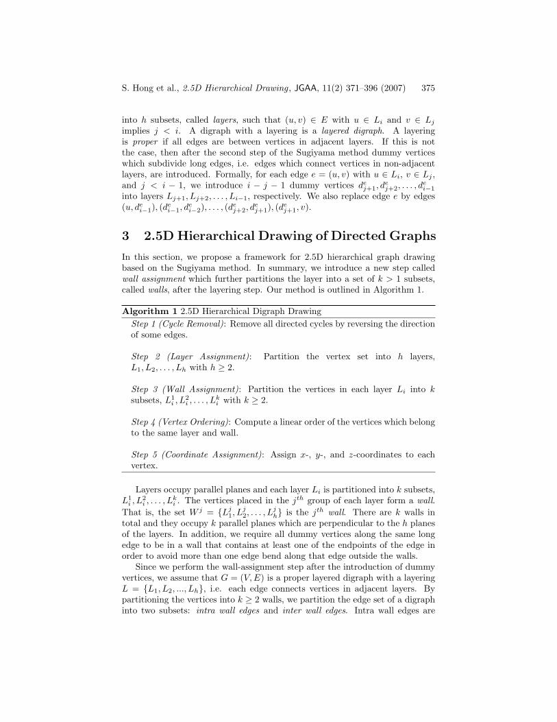
In this section, we propose a framework for 2.5D hierarchical graph drawingbased on the Sugiyama method. In summary, we introduce a new step calledwall assignment which further partitions the layer into a set of k > 1 subsets,called walls, after the layering step. Our method is outlined in Algorithm 1.

Algorithm 1 2.5D Hierarchical Digraph Drawing

Step 1 (Cycle Removal): Remove all directed cycles by reversing the directionof some edges.

Step 2 (Layer Assignment): Partition the vertex set into h layers,L1, L2, . . . , Lh with h ≥ 2.

Step 3 (Wall Assignment): Partition the vertices in each layer Li into ksubsets, L1

i , L2i , . . . , L

ki with k ≥ 2.

Step 4 (Vertex Ordering): Compute a linear order of the vertices which belongto the same layer and wall.

Step 5 (Coordinate Assignment): Assign x-, y-, and z-coordinates to eachvertex.

Layers occupy parallel planes and each layer Li is partitioned into k subsets,L1

i , L2i , . . . , L

ki . The vertices placed in the jth group of each layer form a wall.

That is, the set W j = {Lj1, L

j2, . . . , L

jh} is the jth wall. There are k walls in

total and they occupy k parallel planes which are perpendicular to the h planesof the layers. In addition, we require all dummy vertices along the same longedge to be in a wall that contains at least one of the endpoints of the edge inorder to avoid more than one edge bend along that edge outside the walls.

Since we perform the wall-assignment step after the introduction of dummyvertices, we assume that G = (V,E) is a proper layered digraph with a layeringL = {L1, L2, ..., Lh}, i.e. each edge connects vertices in adjacent layers. Bypartitioning the vertices into k ≥ 2 walls, we partition the edge set of a digraphinto two subsets: intra wall edges and inter wall edges. Intra wall edges are


edges with both endpoints in the same wall, and inter wall edges are edges withendpoints in different walls. The span of an inter wall edge is the absolutevalue of the difference between the numbers of the two walls which contain theendpoints of that edge. Note that each inter wall edge has at least one endpointwhich is not a dummy vertex because we require all dummy vertices along thesame long edge to be in the same wall.

The partition of the original vertex set into k walls may originate from thedigraph’s application domain. They might be the clusters of a given clustereddigraph. If no such partition is given, then the vertex set can be partitionedinto k walls according to the following optimization criteria:

• C1. Even distribution of vertices among walls, i.e. balanced partition ofthe vertex set into walls.

• C2. Minimum number of inter wall edges for avoiding occlusion in the 3Dspace.

• C3. Minimum number of crossings between inter wall edges in the pro-jection of the drawing into a plane which is orthogonal to both the layerplanes and the wall planes. This criterion expresses the desire that interwall edges to be grouped in planes which can only intersect in the walls.

• C4. Minimum total edge length of inter wall edges.

These criteria are designed to express the properties of layouts with lowvisual complexity. They give rise to some hard optimization problems whichrequire the development of efficient algorithms. In the remainder of this section,we propose a few alternative wall-assignment algorithms which are designed tosatisfy different subsets of the listed optimization criteria.

3.1 Two-Wall Partitions Based on Minimum Bisection

The minimum number of walls in a 2.5D hierarchical layout is two. The specialcase of having only two walls is interesting because it combines the advantagesof our 2.5D drawing convention with a simple presentation that helps to pre-vent occlusion. In this and the following sections, we propose two alternativeapproaches to two-wall assignment according to different optimization criteria.

To find a partition of the vertex set into two walls according to criteria C1

and C2 is a special case of the well-known minimum b-balanced cut problemfor b = 1/2. For a given undirected graph G = (V,E) and a subset of verticesC ⊆ V , the cut (C, V \ C) is the set of all edges with one endpoint in C andone endpoint in V \ C. Let w : V → N and c : E → N be a vertex-weightand an edge cost function, respectively. The minimum b-balanced cut problemis the problem of finding a cut (C, V \ C) with the minimum total edge cost,such that min{w(C), w(V − C)} ≥ b.w(V ) for a given positive b ≤ 1/2. Whenb = 1/2 and c(e) = 1 for each e ∈ E, the problem is also known as the minimumbisection problem. This is the same problem that has to be solved if the vertexset is partitioned into two walls according to criteria C1 and C2.


The minimum bisection problem is NP-hard [16]. Various heuristic and ap-proximation algorithms have been proposed for solving it (see [21, 14, 24, 13]) thelatest of which is the divide and conquer algorithm by Feige and Krauthgamerwhich finds a bisection with a cost within ratio of O(log1.5 n) from the minimumin polynomial time [12].

The first wall-assignment algorithm that we propose solves the minimumbisection problem heuristically. It is a simplistic approach to minimum bisectioncompared to the algorithm of Feige and Krauthgamer, but it is specificallydesigned for use within the Sugiyama framework. When assigning vertices towalls according to C1 and C2, additional requirements may take higher prioritythan the exact separation of the vertex set into two equal-size halves with theexact minimum number of edges between them. Such an additional requirement,for example, is to have all dummy vertices along the same edge assigned to thesame wall. It is also very important for a wall-assignment algorithm to run fastbecause it is only a part of a five-step framework.

We propose to assign vertices to walls layer by layer starting with the firstlayer. For this purpose, we define the minimum one-layer bisection problem asfollows.

Minimum One-Layer Bisection Problem

Consider two adjacent layers Li−1 and Li. Let Li−1 be partitioned into subsetsAi−1 and Bi−1. Find a partition of Li into subsets Ai and Bi such that||Ai| − |Bi|| ≤ 1 and the number of edges between Ai−1 and Bi plus thenumber of edges between Ai and Bi−1 is the minimum.

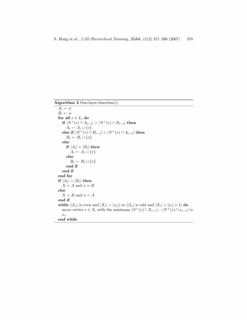
We propose a greedy algorithm, Algorithm 2, which solves the one-layerbisection problem optimally. It has two phases; at the first phase each vertex inlayer Li is assigned to the wall that contains the biggest number of its immediatesuccessors; at the second phase some vertices are moved from one wall to theother in order to achieve a balanced partition.

Theorem 1 For given i, Ai−1, and Bi−1, Algorithm 2 partitions layer Li intoAi and Bi so that:

Property 1: |Ai| = |Bi| if |Li| is even, and ||Ai| − |Bi|| = 1 if |Li| is odd.Property 2: The number of inter wall edges between Ai−1∪Ai and Bi−i∪Bi

is the minimum for a partition with Property 1.

Proof: Property 1 is trivially implied by the while loop. Assume there existsanother partition of layer Li into subsets A′

i and B′i which satisfy both Prop-

erty 1 and Property 2. We will show that the partition defined by A′i and B′

i

must have the same number of inter wall edges as the partition defined by Ai

and Bi.Without loss of generality, assume that |Ai| ≥ |Bi| before the while loop

in Algorithm 2 and let Ci be the set of vertices moved from Ai to Bi after theexecution of the while loop. Let also Abefore

i and Aafteri denote Ai before and

after the while loop, respectively. Similarly, let Bbeforei and Bafter

i denote Bi

before and after the while loop, respectively.


Algorithm 2 One-layer-bisection(i)

Ai ← φBi ← φfor all v ∈ Li do

if |N+(v) ∩Ai−1| > |N+(v) ∩Bi−1| then

Ai ← Ai ∪ {v}else if |N+(v) ∩Bi−1| > |N

+(v) ∩Ai−1| then

Bi ← Bi ∪ {v}else

if |Ai| < |Bi| then

Ai ← Ai ∪ {v}else

Bi ← Bi ∪ {v}end if

end if

end for

if |Ai| > |Bi| then

X = A and x = Belse

X = B and x = Aend if

while (|Li| is even and |Xi| > |xi|) or (|Li| is odd and |Xi| > |xi|+ 1) do

move vertex v ∈ Xi with the minimum |N+(v)∩Xi−1| − |N+(v)∩ xi−1| to

xi

end while


Figure 2: A 2.5D hierarchical layout with a wall partition based on minimumbisection.

Case 1. There is a vertex v ∈ A′i ∩Bbefore

i . By moving v to B′i, we subtract

from the number of inter wall edges |N+(v) ∩Bi−1| − |N+(v) ∩Ai−1| ≥ 0. Let

A′′i = A′

i \ {v} and B′′i = B′

i ∪ {v}. If A′′i and B′′

i do not satisfy Property 1

because B′′i is too large, then clearly |B′′

i | > |Bbeforei | and there is a vertex

u ∈ B′′i ∩ Abefore

i which can be moved to A′′i to satisfy Property 1 without

increasing the number of inter wall edges. If the number of inter wall edgesdecreases, this will contradict the assumption that the partition (A′

i, B′i) has

the minimum number of inter wall edges. Otherwise we can repeat the sameconsiderations until we end up with A′′

i ∩ Bbeforei = φ. Then we continue with

the considerations in case 2.Case 2. A′

i ⊆ Abeforei . If A′

i is different from Aafteri , then B′

i ∩ Aafteri is

not empty. Let v ∈ B′i ∩ Aafter

i . By moving v to A′i, we will subtract from

the number of inter wall edges α = |N+(v) ∩ Ai−1| − |N+(v) ∩ Bi−1| ≥ 0.

(Note that Aafter ⊆ Abefore.) Let A′′i ← A′

i ∪ {v} and B′′i ← B′

i \ {v}. IfA′′

i and B′′i do not satisfy Property 1 because A′′

i is too large, then clearly

|A′′i | > |Aafter

i | and there is a vertex u ∈ Ci ∪ A′′i which is different from v

and β = |N+(u) ∩ Ai−1| − |N+(u) ∩ Bi−1| ≤ α. Let A′′′

i ← A′′i \ {u} and

B′′′i ← B′′

i ∪ {u}. The partition (A′′′i , B′′′

i ) has α− β ≥ 0 fewer inter wall edges

than the partition (A′i, B

′i). If A′′′

i is different from Aafteri , we can repeat the

considerations for A′′′i and B′′′

i . Since this procedure cannot repeat forever, it

will eventually end up with A′′′i = Aafter

i . 2

For partitioning the whole vertex set into two walls, we propose to partitionthe first layer into two halves randomly and then apply Algorithm 2 for all layersfrom L2 to Lh layer by layer. An example layout is shown in Figure 2.

The for loop takes O(|V |+ |E|) time in total because each vertex and edgeare scanned once. The while loop can take additional O(|V | log |V |) time in


total if Ai and Bi are sorted lists implemented efficiently, e.g. by Fibonacciheaps. Thus, the total worst-case time complexity of running Algorithm 2 forall layers from L2 to Lh is O(|V | log |V |+ |E|).

Lemma 1 The total worst-case time complexity of running Algorithm 2 for alllayers from L2 to Lh is O(|V | log |V |+ |E|).

Since some layers may have an odd number of vertices, Algorithm 2 cannotguarantee that the vertices will be equally split between the two walls. Howeverthe balance is good enough for the purpose of hierarchical digraph drawingand our computational study in Section 4 shows evidence that the algorithmguarantees a relatively low total number of inter wall edges by working optimallyon the two-layer scale.

Note that the described method does not necessarily place all dummy ver-tices along the same edge in the same wall. In order to enforce it, we need toforbid the movement of dummy vertices in the while loop in Algorithm 2. Thatmay worsen the balance of the partition, but it may also reduce the number ofinter wall edges.

3.2 Two-Wall Partitions with Specific Arrangements of

Inter Wall Edges

The following two algorithms for partitioning the vertex set into two walls aredesigned to have all inter wall edges arranged in a particular pattern such thatC3 is satisfied. We call them zig-zag wall partition and dominating-wall parti-tion respectively.

Both algorithms scan all layers one by one from bottom to top and partitioneach of them into two subsets. We start with a random balanced partitionof the first layer. Each next layer Li is partitioned into L1

i and L2i such that

L1i ∪ L2

i = Li and L1i ∩ L2

i = φ based on the partition of layer Li−1.In both algorithms this is performed by the procedure DIVIDELAYER(i, x, y)

which sets Lxi ← {v ∈ Li : N+(v) ∩ Ly

i−1 = φ} and Lyi ← Li \ Lx

i .Algorithm 3 presents the zig-zag wall partition, and algorithm 4 presents the

dominating-wall partition. Example layouts are shown in Figures 3 and 4.

Algorithm 3 Zig-zag wall partition

Partition L1 randomly into two halves.for i = 2..h do

if i mod 2 = 0 then

DIVIDELAYER(i, 1, 2)else

DIVIDELAYER(i, 2, 1)end if

end for


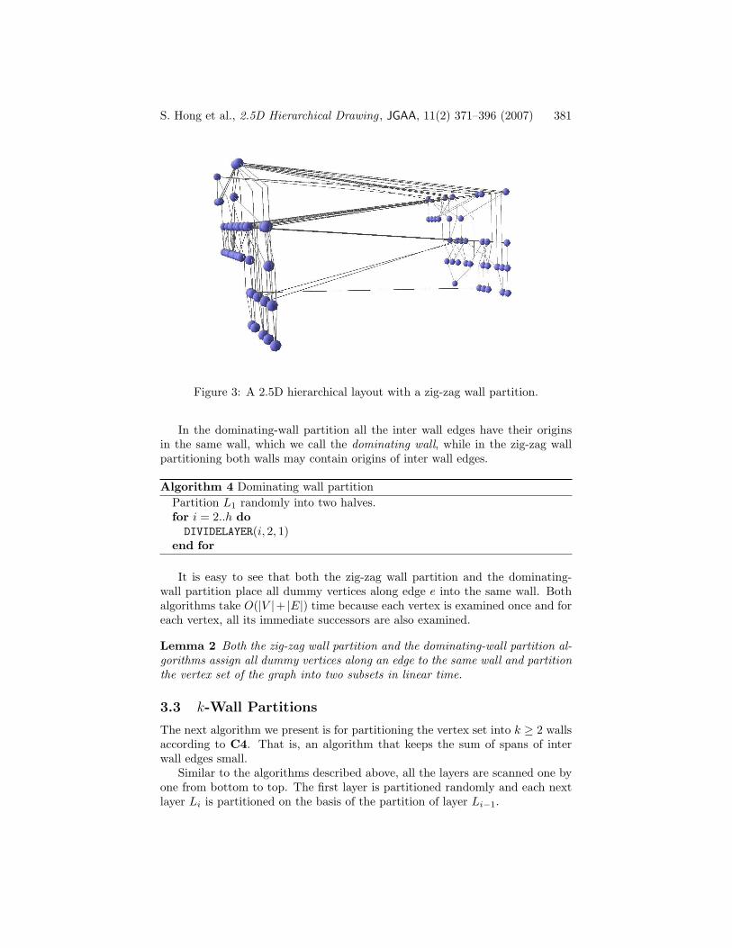
Figure 3: A 2.5D hierarchical layout with a zig-zag wall partition.

In the dominating-wall partition all the inter wall edges have their originsin the same wall, which we call the dominating wall, while in the zig-zag wallpartitioning both walls may contain origins of inter wall edges.

Algorithm 4 Dominating wall partition

Partition L1 randomly into two halves.for i = 2..h do

DIVIDELAYER(i, 2, 1)end for

It is easy to see that both the zig-zag wall partition and the dominating-wall partition place all dummy vertices along edge e into the same wall. Bothalgorithms take O(|V |+ |E|) time because each vertex is examined once and foreach vertex, all its immediate successors are also examined.

Lemma 2 Both the zig-zag wall partition and the dominating-wall partition al-gorithms assign all dummy vertices along an edge to the same wall and partitionthe vertex set of the graph into two subsets in linear time.

3.3 k-Wall Partitions

The next algorithm we present is for partitioning the vertex set into k ≥ 2 wallsaccording to C4. That is, an algorithm that keeps the sum of spans of interwall edges small.

Similar to the algorithms described above, all the layers are scanned one byone from bottom to top. The first layer is partitioned randomly and each nextlayer Li is partitioned on the basis of the partition of layer Li−1.


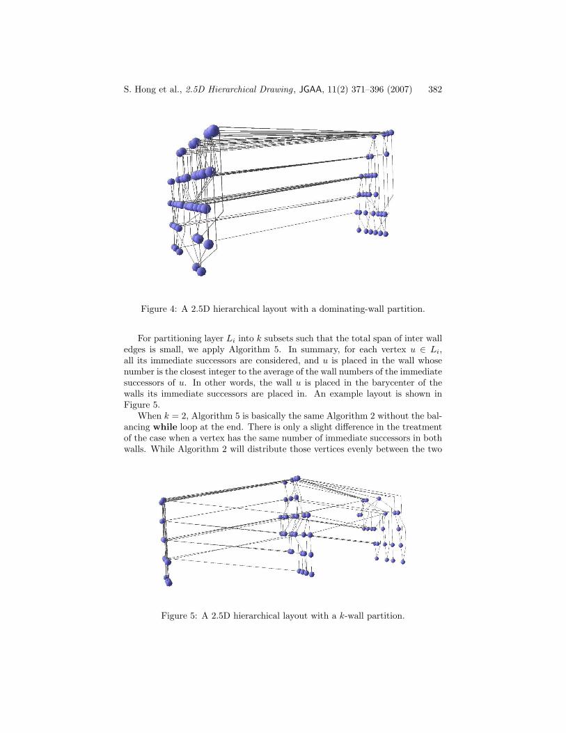
Figure 4: A 2.5D hierarchical layout with a dominating-wall partition.

For partitioning layer Li into k subsets such that the total span of inter walledges is small, we apply Algorithm 5. In summary, for each vertex u ∈ Li,all its immediate successors are considered, and u is placed in the wall whosenumber is the closest integer to the average of the wall numbers of the immediatesuccessors of u. In other words, the wall u is placed in the barycenter of thewalls its immediate successors are placed in. An example layout is shown inFigure 5.

When k = 2, Algorithm 5 is basically the same Algorithm 2 without the bal-ancing while loop at the end. There is only a slight difference in the treatmentof the case when a vertex has the same number of immediate successors in bothwalls. While Algorithm 2 will distribute those vertices evenly between the two

Figure 5: A 2.5D hierarchical layout with a k-wall partition.


Algorithm 5 Barycenter k-wall partition of layer Li

for all j = 1..k do

Lji ← φ

end for

for all u ∈ Li do

if |N+(u)| = 0 then

Let b be a number such that |Lbi | = min{|L1

i |, |L2i |, . . . , |L

ki |}

else

for all j = 1..k do

neighbours[j]← |N+(u) ∩ Lji−1|

end for

b←⌊

∑ kj=1

j∗neighbours[j]∑

kj=1

neighbours[j]+ 0.5

⌋

end if

Lbi ← Lb

i ∪ {u}end for

walls, Algorithm 5 will place all of them in the same wall.Clearly, the proposed algorithm while keeping the number of inter wall edges

low does not guarantee balanced distribution of the vertices among the walls.The problem of balanced partitioning the vertex set of a graph into k ≥ 2 subsetswith the minimum number of edges between the subsets is a generalization of theNP-hard minimum bisection problem discussed in Section 3.1. It is known as the(k, ν)-balanced partitioning problem where each subset is required to have size

at most ν∗ |V |k

. In a recent study, Andreev and Racke have shown that the (k, 1)-balanced partitioning problem has no polynomial time approximation algorithmwith finite approximation factor unless P = NP , and propose a polynomialtime algorithm for solving the (k, 1 + ǫ)-balanced partitioning problem with anO(log2 |V |/ǫ4) approximation ratio [3].

In order to achieve a more even distribution of vertices between the walls,i.e. to satisfy C1, we propose a technique which is simpler compared to thealgorithm of Andreev and Racke [3], but it runs in linear time and our com-putational study gives evidence that it achieves a good enough balance. Ourmethod is the following. When computing the barycenter value b, we alternateit for giving preference to the walls with fewer number of vertices.

The implementation of such a procedure is presented in Algorithm 6, whichis a generalised version of Algorithm 5. Now the wall for vertex u is computedas

b =

⌊

∑k

j=1 j ∗max{0, neighbours[j]− |Lji |}

∑k

j=1 max{0, neighbours[j]− |Lji |}

+ 0.5

⌋

. (1)

in the case∑k

j=1 max{0, neighbours[j] − |Lji |} > 0. Otherwise, u is placed in

the wall with the fewest number of vertices in the current layer. An examplelayout is shown in Figure 6.

It is easy to see that Algorithm 5 guarantees that all dummy vertices along


Figure 6: A 2.5D hierarchical layout with a balanced k-wall partition.

Algorithm 6 Balanced barycenter k-wall partition of layer Li

for all j = 1..k do

Lji ← φ

end for

for all u ∈ Li do

if u is a dummy vertex then

Let b be the number such that the only immediate successor of u isassigned to Lb

i−1.else

for all j = 1..k do

neighbours[j]← |N+(v) ∩ Lji−1|

end for

if∑k

j=1 max{0, neighbours[j]− |Lji |} > 0 then

b←

⌊

∑ kj=1

j∗max{0,neighbours[j]−|Lj

i|}

∑

kj=1

max{0,neighbours[j]−|Lj

i|}

+ 0.5

⌋

else

Let b be a number such that |Lbi | = min{|L1

i |, |L2i |, . . . , |L

ki |}

end if

end if

Lbi ← Lb

i ∪ {u}end for


an edge belong to the same wall. However, this is no longer guaranteed withthe balancing technique in Algorithm 6. Thus, when applying the balancingtechnique, we first need to check whether u is dummy and if it is then assign itto the wall of its immediate successor.

The time complexity of the proposed k-wall partitioning algorithm is alsoO(|V |+ |E|) because each vertex and each edge are scanned once.

Lemma 3 Both versions of the k-wall partition algorithm assign all dummyvertices along an edge to the same wall, and partition the vertex set of the graphinto k ≥ 2 subsets in linear time.

4 Computational Results

In our experimental work we used 5911 DAGs from the well-known Rome graphdataset introduced by di Battista et al. in their experimental studies [8] andavailable at the GDToolkit website2. The copy of the Rome graph set we haveconsists of 11,530 graphs in LEDA3 format. Since, by default, a graph in LEDAformat is directed, we accepted the default direction of the edges given by theLEDA format and filtered out the graphs with directed cycles. We also filteredout the unconnected graphs leaving 5911 DAGs. The graphs have vertex countbetween 10 and 100. The x-axis in all the plots below represents the numberof original vertices in a graph. We have partitioned all DAGs into groups byvertex count. Each group covers an interval of size 5 on the x-axis, except thelast group which represents only the graphs with 100 vertices. We display theaverage result for each group. Partitioning the DAGs into groups by edge countreveals the same results because the DAGs typically have twice as many edgesas vertices.

The objective of our computational study was to compare the different wallassignment techniques introduced in Section 3. Note that the k-wall partitiontechniques can be applied for two-wall partitioning as well when k = 2. The firstpart of our computational study compares the two-wall partition techniques, andthe second compares k-wall partitions for different values of k ≥ 2.

To each of the test DAGs, we applied our method (Algorithm 1) with thesame algorithms for all steps except the wall-assignment step. Since the testdigraphs are acyclic, we did not have to remove cycles. For the layer-assignmentstep, we used the network-simplex layering algorithm introduced by Gansner etal. [15]. To be able to compare the number of edge crossings between intra walledges we had to adapt the vertex-ordering step in order to take into accountthe multiple walls.

For the vertex-ordering step, we applied layer-by-layer sweep with the bary-center heuristic for two-layer crossing minimization. In our extended abstracts,we considered ordering the vertices in each wall both independently from otherwalls and taking into account the neighbours of each vertex in other walls. Our

2http://www.dia.uniroma3.it/∼gdt/3http://www.algorithmic-solutions.de/enleda.htm


pilot study gave some evidence that the number of crossings between intra walledges is slightly lower when the vertices in each wall are ordered independentlyfrom other walls [20, 19]. Thus, in the present computational study, we apply thelayer-by-layer sweep for each wall independently. For the computational resultspresented below, we did not have to perform the coordinate assignment step.The example drawings in this paper were made with applying the Brandes-Kopfalgorithm for each wall independently [5].

4.1 Two-Wall Partitions

First we compare the proposed methods for partitioning the vertex set into twowalls. Here we also include the two k-wall methods with k = 2. In the plots,we use the following two-letter references to the wall-assignment methods.

• MB Two Wall-partition based on minimum bisection (Algorithm 2).

• ZZ Zig-zag wall assignment (Algorithm 3).

• DW Dominating-wall assignment (Algorithm 4).

• KW k-wall partition (Algorithm 5).

• BW Balanced k-wall partition (Algorithm 6).

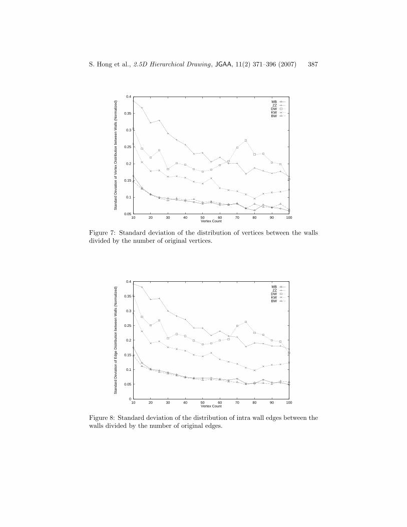
The plot in Figure 7 compares the standard deviation of the distribution ofvertices between the walls. We divided the standard deviation for each DAGby its original vertex count (i.e. before introducing dummy vertices) in order tonormalize it. Similar normalization is applied in all other plots.

As we expected MB and BW have the lowest values which means thatthey have the most balanced distribution of vertices between the walls. Thesame wall-assignment algorithms behave best in terms of distribution of intrawall edges as shown in Figure 8. Figures 7 and 8 also demonstrate that thedistribution of vertices and intra wall edges is not too unbalanced for ZZ, DW,and KW on average. We did not particularly expect this result.

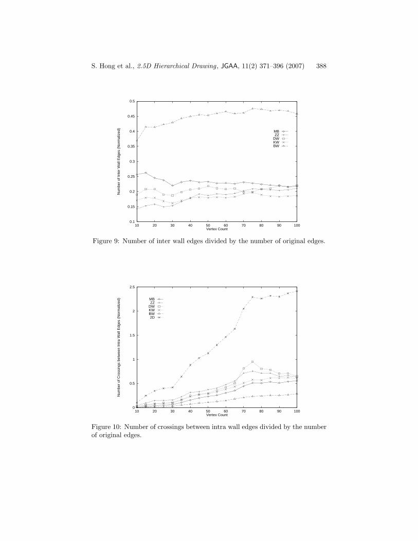
Figure 9 shows that BW has a significantly higher number of inter walledges than any of the other wall-assignment algorithms. KW has the lowestnumber of inter wall edges as we expected, but it is very closely followed by ZZ

and DW. This figure shows that the balancing technique employed by BW istoo simplistic as it fails to keep the number of inter wall edges low.

Finally, Figure 10 compares the number of crossings between intra wall edgesfor all wall assignment methods and the 2D case (i.e. without partitioning intowalls). The low number of edge crossings for BW is due to the high numberof inter wall edges. In general, Figure 10 gives evidence that by partitioning ahierarchy into two walls by any of the proposed methods, the number crossingsbetween intra wall edges can be reduced at least twice.


0.05

0.1

0.15

0.2

0.25

0.3

0.35

0.4

10 20 30 40 50 60 70 80 90 100

Sta

ndar

d D

evia

tion

of V

erte

x D

istr

ibut

ion

betw

een

Wal

ls (

Nor

mal

ized

)

Vertex Count

MBZZ

DWKWBW

Figure 7: Standard deviation of the distribution of vertices between the wallsdivided by the number of original vertices.

0

0.05

0.1

0.15

0.2

0.25

0.3

0.35

0.4

10 20 30 40 50 60 70 80 90 100

Sta

ndar

d D

evia

tion

of E

dge

Dis

trib

utio

n be

twee

n W

alls

(N

orm

aliz

ed)

Vertex Count

MBZZ

DWKWBW

Figure 8: Standard deviation of the distribution of intra wall edges between thewalls divided by the number of original edges.


0.1

0.15

0.2

0.25

0.3

0.35

0.4

0.45

0.5

10 20 30 40 50 60 70 80 90 100

Num

ber

of In

ter

Wal

l Edg

es (

Nor

mal

ized

)

Vertex Count

MBZZ

DWKWBW

Figure 9: Number of inter wall edges divided by the number of original edges.

0

0.5

1

1.5

2

2.5

10 20 30 40 50 60 70 80 90 100

Num

ber

of C

ross

ings

bet

wee

n In

tra

Wal

l Edg

es (

Nor

mal

ized

)

Vertex Count

MBZZ

DWKWBW2D

Figure 10: Number of crossings between intra wall edges divided by the numberof original edges.


0.05

0.1

0.15

0.2

0.25

0.3

10 20 30 40 50 60 70 80 90 100

Sta

ndar

d D

evia

tion

of V

erte

x D

istr

ibut

ion

betw

een

Wal

ls (

Nor

mal

ized

)

Vertex Count

k=2k=3k=4k=5

Figure 11: Standard deviation of the distribution of vertices between the wallsdivided by the number of original vertices.

4.2 k-Wall Partitions

Our study for k = 2 as well as our practical experience with k > 2 showedevidence that BW while achieving balanced partitioning has a higher numberof inter wall edges than KW. In this section we study the behavior only of KW

for different values of k.Figures 11 and 12 demonstrate that the distribution of vertices and intra wall

edges does not depend on the number of walls too heavily. It can be expectedthat the distribution becomes more balanced with increasing the number ofwalls. However, with the growth of the number of walls, grows the number ofinter wall edges and their total span, as seen in Figures 13 and 14. Based onthis evidence, we would suggest partitioning of digraphs with up to 100 verticesinto no more than four walls. Figure 15 shows the maximum number of edgesbetween adjacent walls, i.e. the maximum edge density between the walls. It canbe observed that it does not depend on the number of walls for the considereddataset and values of k.

We also experimented with partitioning the vertex set of each DAG intowalls whose count depends on the size of the vertex set. For this purpose, weset the number of walls at max{2, n/30}, where n is the total number of originaland dummy vertices in the DAG. Figure 16 presents the average number of wallsfor our dataset. Figure 17 shows an interesting result. It compares the numberof crossings between intra wall edges in KW to the number of edge crossings in2D layouts. While the average number of edge crossings grows with the growthof the size of the graph in the 2D layouts, it is virtually constant in the KW

layouts when the number of walls depends on the size of the graph.


0.05

0.1

0.15

0.2

0.25

0.3

10 20 30 40 50 60 70 80 90 100

Sta

ndar

d D

evia

tion

of E

dge

Dis

trib

utio

n be

twee

n W

alls

(N

orm

aliz

ed)

Vertex Count

k=2k=3k=4k=5

Figure 12: Standard deviation of the distribution of intra wall edges betweenthe walls divided by the number of original edges.

0.15

0.2

0.25

0.3

0.35

0.4

0.45

0.5

10 20 30 40 50 60 70 80 90 100

Num

ber

of In

ter

Wal

l Edg

es (

Nor

mal

ized

)

Vertex Count

k=2k=3k=4k=5

Figure 13: Number of inter wall edges divided by the number of original edges.


0.15

0.2

0.25

0.3

0.35

0.4

0.45

0.5

0.55

0.6

10 20 30 40 50 60 70 80 90 100

Tot

al S

pan

of In

ter

Wal

l Edg

es (

Nor

mal

ized

)

Vertex Count

k=2k=3k=4k=5

Figure 14: Total span of the inter wall edges divided by the number of originaledges.

0.15

0.16

0.17

0.18

0.19

0.2

0.21

10 20 30 40 50 60 70 80 90 100

Max

imum

Edg

e D

ensi

ty b

etw

een

Wal

ls (

Nor

mal

ized

)

Vertex Count

k=2k=3k=4k=5

Figure 15: Maximum number of edges between adjacent walls divided by thenumber of original edges.


2

3

4

5

6

7

8

10 20 30 40 50 60 70 80 90 100

Num

ber

of W

alls

Vertex Count

KW

Figure 16: Variable number of walls in KW layouts dependent on the size ofthe DAG.

0

0.5

1

1.5

2

2.5

10 20 30 40 50 60 70 80 90 100

Num

ber

of E

dge

Cro

ssin

gs b

etw

een

Intr

a W

all E

dges

(N

orm

aliz

ed)

Vertex Count

KW2D

Figure 17: Number of crossings between intra wall edges in 2D layouts and inKW layouts with number of walls dependent on the size of the DAG.


5 Conclusions

We introduce a framework for 2.5D hierarchical graph drawing based on theSugiyama method. We propose to partition the vertex set into k ≥ 2 parallelplanes, called walls; each wall containing a 2D drawing of a layered digraph. Thisis done by introducing an additional wall assignment step into the Sugiyamamethod after the layer assignment step.

We propose five alternative fast wall-assignment algorithms and evaluatethem in an extensive computational study with a large dataset. The choice ofa particular wall assignment algorithm may highly depend on the interactionand navigation techniques used for visualizing the layout [2]. We were able toshow evidence that four of the proposed wall-assignment methods perform wellin practice in terms of various properties of the corresponding 2.5D layouts.

Additional improvement in the proposed 2.5D layouts may come from vertex-ordering and coordinate-assignment algorithms specifically developed for 2.5Dhierarchical layouts. Another direction of future research might be related todefining new optimization problems arising from 3D drawing aesthetic criteria.

Acknowledgments

The authors would like to thank Michael Forster for the valuable discussion andsuggestions, and to the whole GEOMI team for implementing our algorithms.


References

[1] A. Ahmed, T. Dwyer, M. Forster, X. Fu, J. Ho, S.-H. Hong, D. Koschutzki,C. Murray, N. S. Nikolov, R. Taib, A. Tarassov, and K. Xu. GEOMI:GEOmetry for Maximum Insight. In P. Healy and N. S. Nikolov, editors,Graph Drawing, 13th International Symposium, GD 2005, volume 3843 ofLecture Notes in Computer Science, pages 468–479. Springer-Verlag, 2005.

[2] A. Ahmed and S.-H. Hong. Navigation techniques for 2.5D graph layout.In Proceedings of APVIS 2007 (Asia-Pacific Symposium on InformationVisualisation). IEEE, to appear.

[3] K. Andreev and H. Racke. Balanced graph partitions. In Proc. of the 16thSPAA, pages 120–124, 2004.

[4] T. Biedl, T. Thiele, and D. R. Wood. Three-dimensional orthogonal graphdrawing with optimal volume. In J. Marks, editor, Graph Drawing: Pro-ceedings of 8th International Symposium, GD 2000, volume 1984 of LectureNotes in Computer Science, pages 284–295. Springer-Verlag, 2001.

[5] U. Brandes and B. Kopf. Fast and simple horizontal coordinate assignment.In P. Mutzel, M. Junger, and S. Leipert, editors, Graph Drawing: Proceed-ings of 9th International Symposium, GD 2001, volume 2265 of LectureNotes in Computer Science, pages 31–44. Springer-Verlag, 2002.

[6] R. Cohen, P. Eades, T. Lin, and F. Ruskey. Three dimensional graphdrawing. Algorithmica, 17(2):199–208, 1996.

[7] G. Di Battista, P. Eades, R. Tamassia, and I. G. Tollis. Graph Drawing.Prentice Hall, 1999.

[8] G. Di Battista, A. Garg, G. Liotta, R. Tamassia, E. Tassinari, andF. Vargiu. An experimental comparison of four graph drawing algorithms.Computational Geometry: Theory and Applications, 7:303–316, 1997.

[9] V. Dujmovic, P. Morin, and D. R. Wood. Path-width and three-dimensionalstraight-line grid drawing of graphs. In M. Goodrich and S. Koburov,editors, Graph Drawing: Proceedings of 10th International Symposium, GD2002, volume 2528 of Lecture Notes in Computer Science, pages 42–53.Springer-Verlag, 2002.

[10] P. Eades and K. Sugiyama. How to draw a directed graph. Journal ofInformation Processing, 13(4):424–437, 1990.

[11] P. Eades, A. Symvonis, and S. Whitesides. Three dimensional orthogonalgraph drawing algorithms. Discrete Applied Mathematics, 103:55–87, 2000.

[12] U. Feige and R. Krauthgamer. A polylogarithmic approximation of theminimum bisection. SIAM J. Comput, 31(4):1090–1118, 2002.


[13] U. Feige, R. Krauthgamer, and K. Nissim. Approximating the minimumbisection size. In Proceedings of the 32nd ACM Symposium on Theory ofComputing (STOC), pages 530–536, 2000.

[14] C. M. Fiduccia and R. M. Mattheyses. A linear time heuristic for improvingnetwork partitions. In Proceedings of the 19th IEEE Design AutomationConference, pages 175–181, 1982.

[15] E. R. Gansner, E. Koutsofios, S. C. North, and K.-P. Vo. A techniquefor drawing directed graphs. IEEE Transactions on Software Engineering,19(3):214–230, March 1993.

[16] M. R. Garey and D. S. Johnson. Computers and Intractability: A Guideto the Theory of NP-Completeness. W. H. Freeman, New York, 1979.

[17] A. Garg and R. Tamassia. GIOTTO: A system for visualizing hierarchicalstructures in 3D. In S. North, editor, Graph Drawing: Symposium on GraphDrawing, GD ’96, volume 1190 of Lecture Notes in Computer Science, pages193–200. Springer-Verlag, 1997.

[18] S.-H. Hong. Drawing graphs symmetrically in three dimensions. InP. Mutzel, M. Junger, and S. Leipert, editors, Graph Drawing: Proceed-ings of 9th International Symposium, GD 2001, volume 2265 of LectureNotes in Computer Science, pages 189–204. Springer-Verlag, 2002.

[19] S.-H. Hong and N. S. Nikolov. Hierarchical layouts of directed graphs inthree dimensions. In P. Healy and N. S. Nikolov, editors, Graph Drawing,13th International Symposium, GD 2005, volume 3843 of Lecture Notes inComputer Science, pages 251–261. Springer-Verlag, 2005.

[20] S.-H. Hong and N. S. Nikolov. Layered drawings of directed graphs in threedimensions. In S.-H. Hong, editor, Information Visualisation 2005: Asia-Pacific Symposium on Information Visualisation (APVIS2005), volume 45,pages 69–74. CRPIT, 2005.

[21] B. W. Kernigham and S. Lin. An efficient heuristic procedure for parti-tioning graphs. Bell System Technical Journal, 49(2):291–308, 1970.

[22] D. Ostry. Some three-dimensional graph drawing algorithms. Master’sthesis, University of Newcastle, 1996.

[23] J. Pach, T. Thiele, and G. Toth. Three-dimensional grid drawings of graphs.In G. Di Battista, editor, Graph Drawing: Proceedings of 5th InternationalSymposium, GD 1997, volume 1353 of Lecture Notes in Computer Science,pages 47–51. Springer-Verlag, 1998.

[24] H. Saran and V. V. Vazirani. Finding k cuts within twice the optimal.SIAM J. Comput., 24(1):101–108, 1995.


[25] K. Sugiyama, S. Tagawa, and M. Toda. Methods for visual understandingof hierarchical system structures. IEEE Transaction on Systems, Man, andCybernetics, 11(2):109–125, February 1981.

[26] C. Ware and G. Franck. Viewing a graph in a virtual reality display is threetimes as good as a 2D diagram. In IEEE Conference on Visual Languages,pages 182–183, 1994.

a 2.5d hierarchical drawing of directed...

Documents