hierarchical bayesian modeling using sas procedure mcmc ... · sas+and+winbugs+output+ deviance...
TRANSCRIPT

Hierarchical Bayesian modeling using SAS procedure MCMC:
An Introduction
Ziv Shkedy
Interuniversity Ins,tute for Biosta,s,cs and sta,s,cal Bioinforma,cs CenStat, Hasselt University
Agoralaan 1, B3590 Diepenbeek, Belgium
Bayes2010, May 19-21, 2010

Overview
• Simple comparison between SAS procedure MCMC and Winbugs, 5 examples:
1. Logistic regression model. 2. Model selection using DIC. 3. Diagnostic plot. 4. Hierarchical Bayesian linear model. 5. A change point model.

Example 1:
Proc MCMC – syntax and comparison with Winbugs
Beetles: Example Volume 2 in Winbugs (logis7c regression)

Dose-response modeling for binary data
• Analysis of binary dose response data. • The numbers of beetles killed after 5 hour exposure
to carbon Disulphide. • N=8 different
concentrations.
Beetles: Example Volume 2 in Winbugs (logis7c regression)

Model formulation
Likelihood and linear predictor
Prior models for α and β
Beetles: Example Volume 2 in Winbugs (logis7c regression)

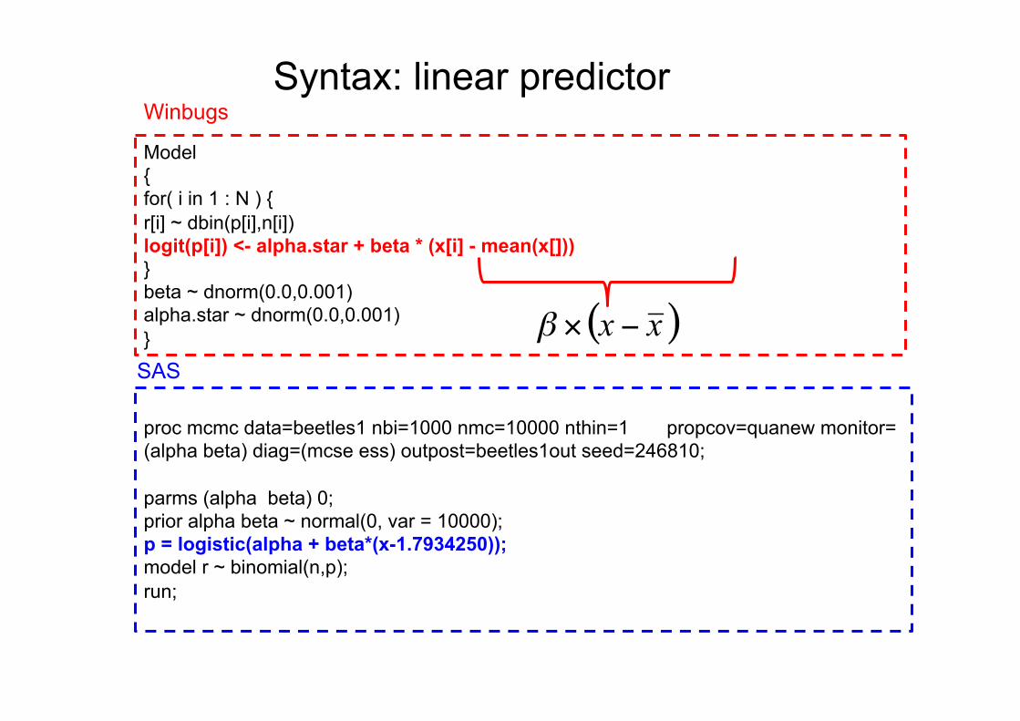
Model { for( i in 1 : N ) { r[i] ~ dbin(p[i],n[i]) logit(p[i]) <- alpha.star + beta * (x[i] - mean(x[])) } beta ~ dnorm(0.0,0.001) alpha.star ~ dnorm(0.0,0.001) }
proc mcmc data=beetles1 nbi=1000 nmc=10000 nthin=1 propcov=quanew monitor=(alpha beta) diag=(mcse ess) outpost=beetles1out seed=246810;
parms (alpha beta) 0; prior alpha beta ~ normal(0, var = 10000); p = logistic(alpha + beta*(x-1.7934250)); model r ~ binomial(n,p); run;
Winbugs
SAS
Syntax: Likelihood

Model { for( i in 1 : N ) { r[i] ~ dbin(p[i],n[i]) logit(p[i]) <- alpha.star + beta * (x[i] - mean(x[])) } beta ~ dnorm(0.0,0.001) alpha.star ~ dnorm(0.0,0.001) }
proc mcmc data=beetles1 nbi=1000 nmc=10000 nthin=1 propcov=quanew monitor=(alpha beta) diag=(mcse ess) outpost=beetles1out seed=246810;
parms (alpha beta) 0; prior alpha beta ~ normal(0, var = 10000); p = logistic(alpha + beta*(x-1.7934250)); model r ~ binomial(n,p); run;
Winbugs
SAS
Syntax: prior models for α and β
Model { for( i in 1 : N ) { r[i] ~ dbin(p[i],n[i]) logit(p[i]) <- alpha.star + beta * (x[i] - mean(x[])) } beta ~ dnorm(0.0,0.001) alpha.star ~ dnorm(0.0,0.001) }
proc mcmc data=beetles1 nbi=1000 nmc=10000 nthin=1 propcov=quanew monitor=(alpha beta) diag=(mcse ess) outpost=beetles1out seed=246810;
parms (alpha beta) 0; prior alpha beta ~ normal(0, var = 10000); p = logistic(alpha + beta*(x-1.7934250)); model r ~ binomial(n,p); run;
Winbugs
SAS
Syntax: linear predictor
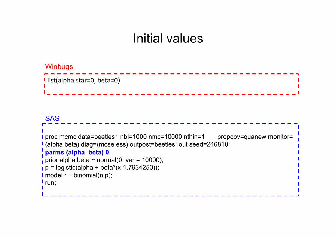
Initial values
list(alpha.star=0, beta=0)
proc mcmc data=beetles1 nbi=1000 nmc=10000 nthin=1 propcov=quanew monitor=(alpha beta) diag=(mcse ess) outpost=beetles1out seed=246810; parms (alpha beta) 0; prior alpha beta ~ normal(0, var = 10000); p = logistic(alpha + beta*(x-1.7934250)); model r ~ binomial(n,p); run;
Winbugs
SAS
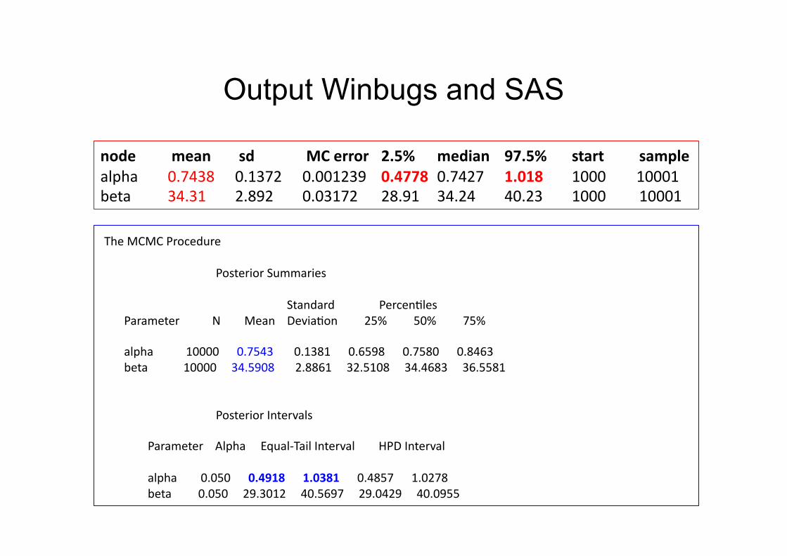
Output Winbugs and SAS
node mean sd MC error 2.5% median 97.5% start sample alpha 0.7438 0.1372 0.001239 0.4778 0.7427 1.018 1000 10001 beta 34.31 2.892 0.03172 28.91 34.24 40.23 1000 10001
The MCMC Procedure
Posterior Summaries
Standard Percen,les Parameter N Mean Devia,on 25% 50% 75%
alpha 10000 0.7543 0.1381 0.6598 0.7580 0.8463 beta 10000 34.5908 2.8861 32.5108 34.4683 36.5581
Posterior Intervals
Parameter Alpha Equal-‐Tail Interval HPD Interval
alpha 0.050 0.4918 1.0381 0.4857 1.0278 beta 0.050 29.3012 40.5697 29.0429 40.0955

proc mcmc data=beetles1 nbi=1000 nmc=10000 nthin=1 propcov=quanew monitor=(alpha beta) diag=(mcse ess) outpost=beetles1out seed=246810;
Options in the proc statement
Burn in period (default=1000)
Number of itera,ons aYer the burn-‐in period
Monitoring every itera,on
Parameter to monitor
In Winbugs: the update tool box and the sample monitor tool.

Example 2: Model Selection using the deviance
information criterion
Beetles: Example Volume 2 in Winbugs (different models for binary data)

Three alternative models for the data
Link function:
Logit
C-log-log
probit
Beetles: Example Volume 2 in Winbugs (different models for binary data)
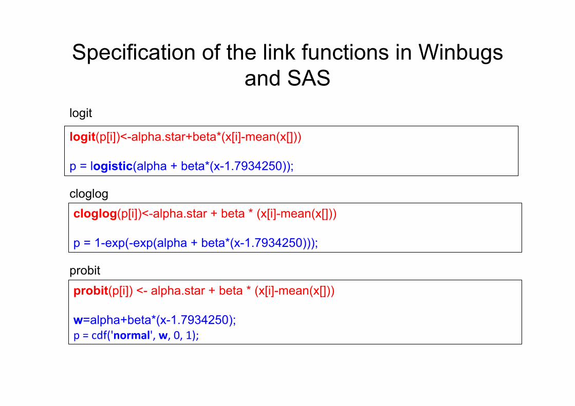
Specification of the link functions in Winbugs and SAS
logit(p[i])<-alpha.star+beta*(x[i]-mean(x[]))
p = logistic(alpha + beta*(x-1.7934250));
cloglog(p[i])<-alpha.star + beta * (x[i]-mean(x[]))
p = 1-exp(-exp(alpha + beta*(x-1.7934250)));
probit(p[i]) <- alpha.star + beta * (x[i]-mean(x[]))
w=alpha+beta*(x-1.7934250); p = cdf('normal', w, 0, 1);
logit
cloglog
probit
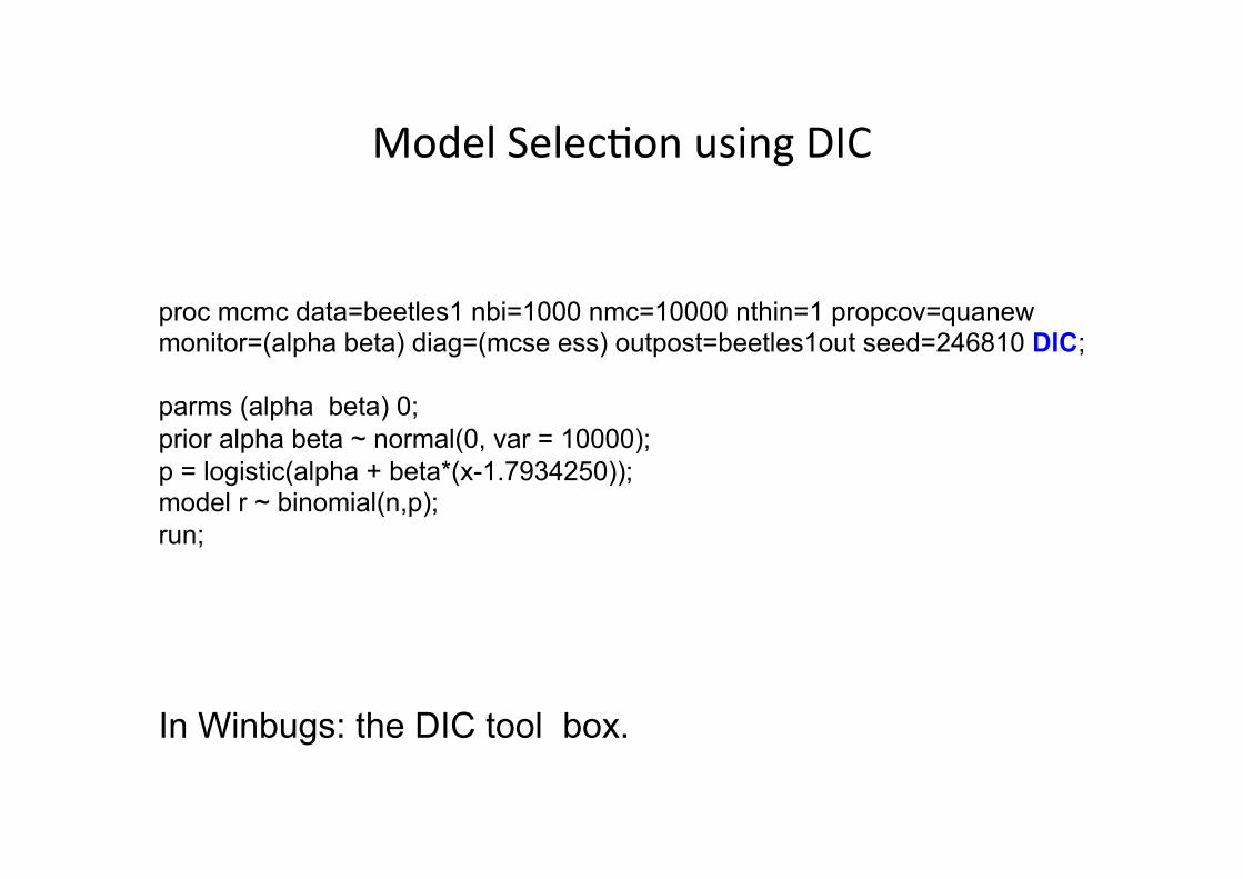
Model Selec,on using DIC
proc mcmc data=beetles1 nbi=1000 nmc=10000 nthin=1 propcov=quanew monitor=(alpha beta) diag=(mcse ess) outpost=beetles1out seed=246810 DIC;
parms (alpha beta) 0; prior alpha beta ~ normal(0, var = 10000); p = logistic(alpha + beta*(x-1.7934250)); model r ~ binomial(n,p); run;
In Winbugs: the DIC tool box.
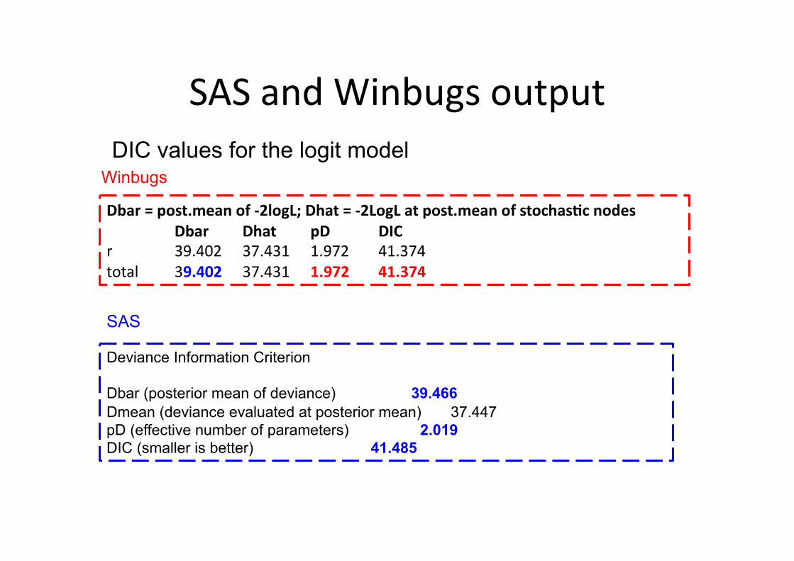
SAS and Winbugs output
Deviance Information Criterion
Dbar (posterior mean of deviance) 39.466 Dmean (deviance evaluated at posterior mean) 37.447 pD (effective number of parameters) 2.019 DIC (smaller is better) 41.485
Dbar = post.mean of -‐2logL; Dhat = -‐2LogL at post.mean of stochas7c nodes Dbar Dhat pD DIC
r 39.402 37.431 1.972 41.374 total 39.402 37.431 1.972 41.374
DIC values for the logit model Winbugs
SAS

DIC, data and posterior means
model DIC SAS DIC WinBUgs
logit 41.485 41.374
c-log-log
33.801 33.715
probit 40.284 40.347

Example 3: Diagnostic plots
Beetles: Example Volume 2 in Winbugs
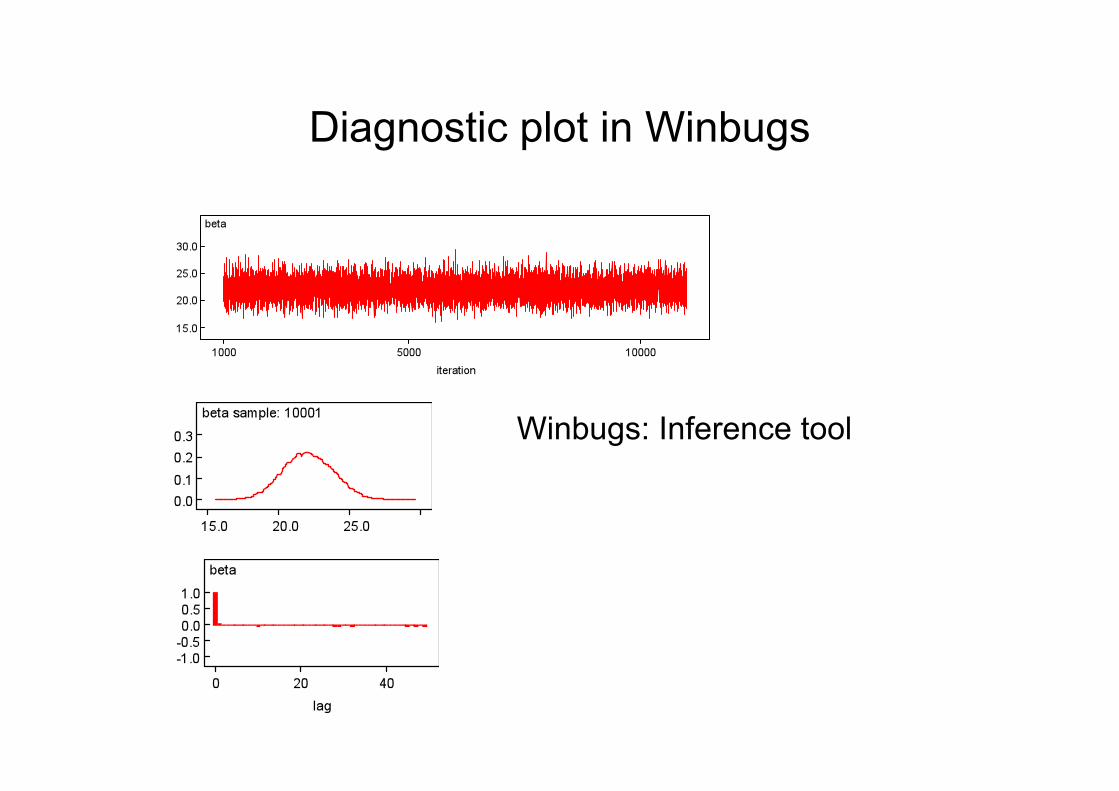
Diagnostic plot in Winbugs
Winbugs: Inference tool
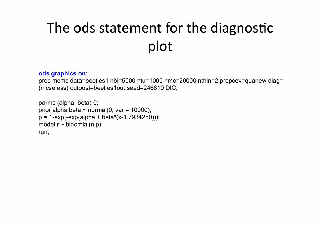
The ods statement for the diagnos,c plot
ods graphics on; proc mcmc data=beetles1 nbi=5000 ntu=1000 nmc=20000 nthin=2 propcov=quanew diag=(mcse ess) outpost=beetles1out seed=246810 DIC;
parms (alpha beta) 0; prior alpha beta ~ normal(0, var = 10000); p = 1-exp(-exp(alpha + beta*(x-1.7934250))); model r ~ binomial(n,p); run;
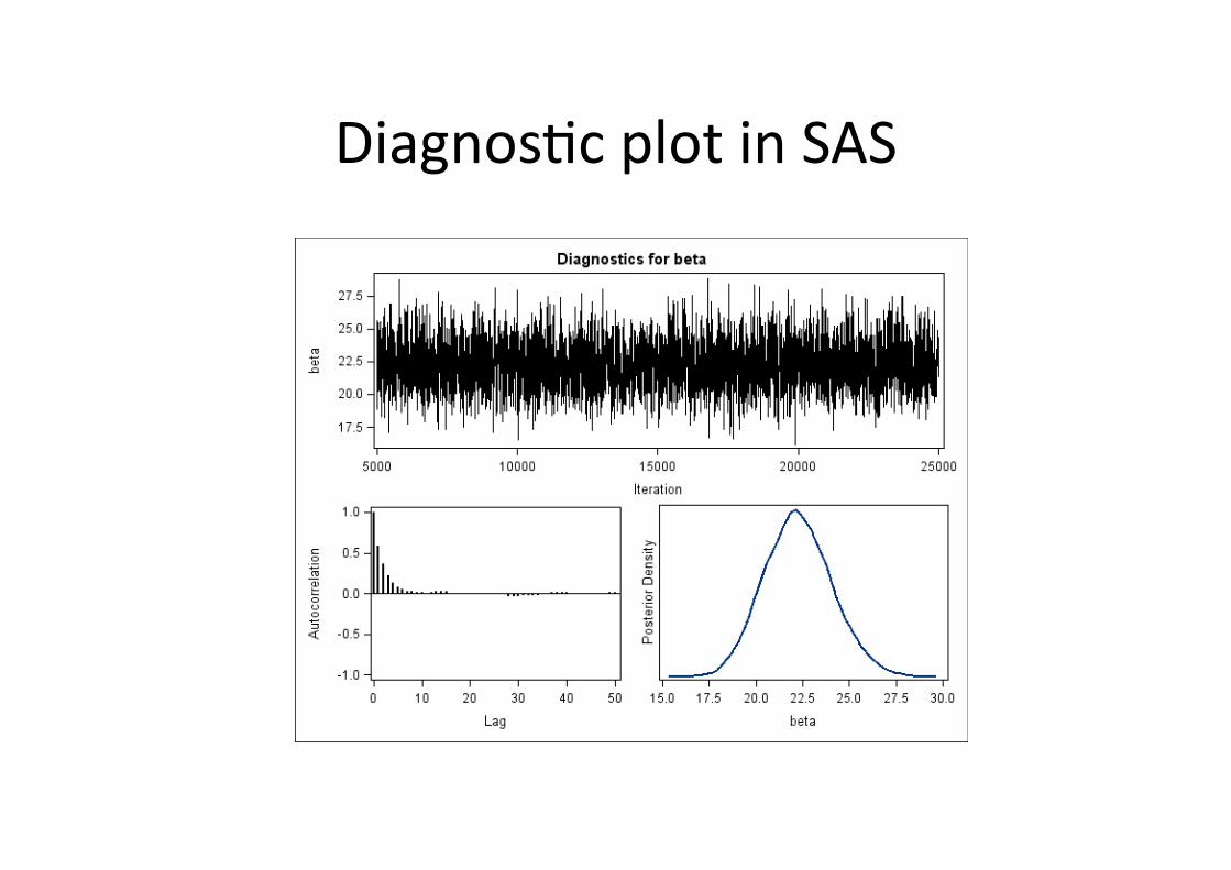
Diagnos,c plot in SAS
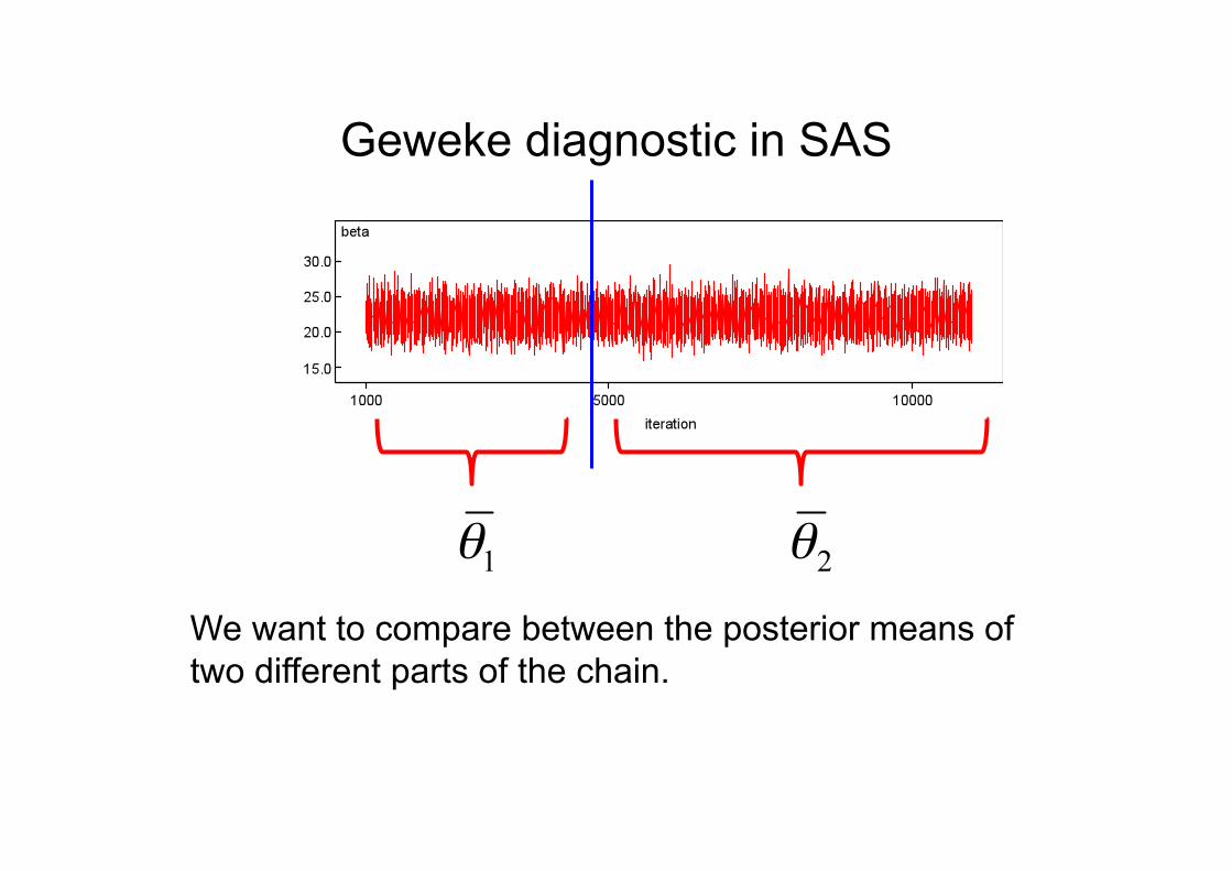
Geweke diagnostic in SAS
We want to compare between the posterior means of two different parts of the chain.
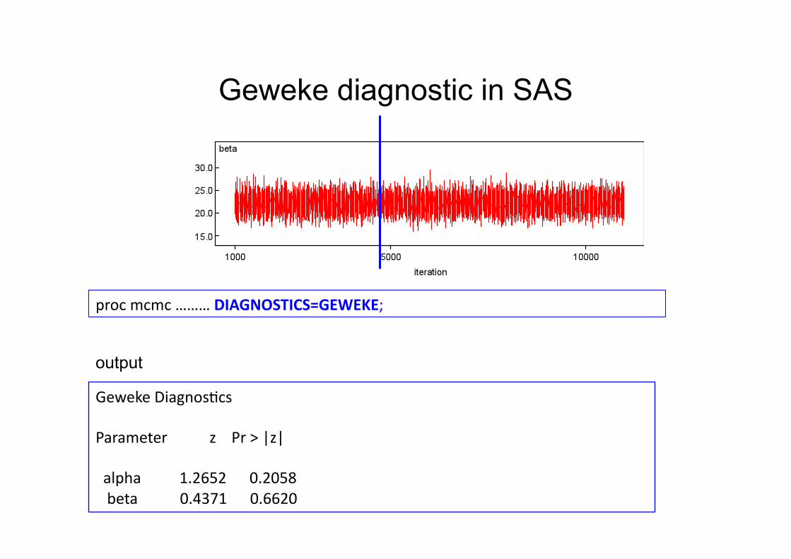
Geweke diagnostic in SAS
proc mcmc ……… DIAGNOSTICS=GEWEKE;
Geweke Diagnos,cs
Parameter z Pr > |z|
alpha 1.2652 0.2058 beta 0.4371 0.6620
output
Example 4: hierarchical linear mixed model
Rats: a normal hierarchical model (Example volume I in winbugs)
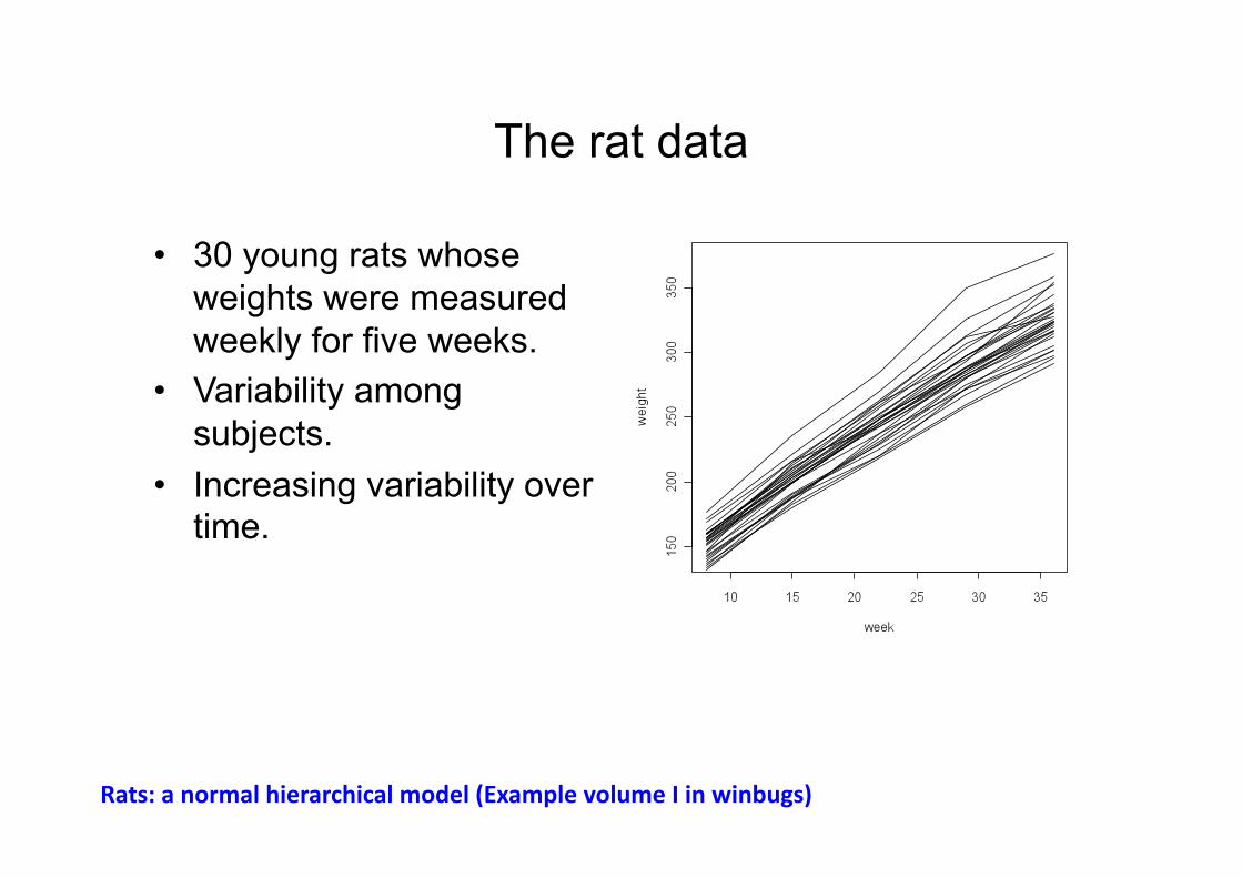
The rat data
• 30 young rats whose weights were measured weekly for five weeks.
• Variability among subjects.
• Increasing variability over time.
Rats: a normal hierarchical model (Example volume I in winbugs)

Model formulation
Linear mixed model with random intercept and random slope:
Rats: a normal hierarchical model (Example volume I in winbugs)
The parameters β0 and β1 are the fixed effects, b0i and b1i are random intercept and slope.

Procedure Mixed: random intercept and random slope
proc mixed data=rat; class id; model y=time/s; repeated id/type=simple; random intercept time/subject=id type=simple; run;
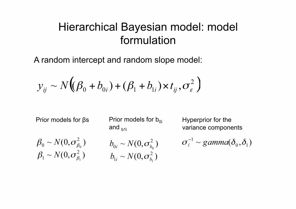
Hierarchical Bayesian model: model formulation
A random intercept and random slope model:
Prior models for βs Prior models for b0i and b1i
Hyperprior for the variance components
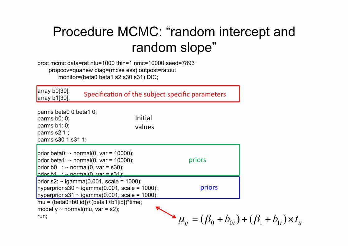
Procedure MCMC: “random intercept and random slope”
proc mcmc data=rat ntu=1000 thin=1 nmc=10000 seed=7893 propcov=quanew diag=(mcse ess) outpost=ratout monitor=(beta0 beta1 s2 s30 s31) DIC;
array b0[30]; array b1[30];
parms beta0 0 beta1 0; parms b0: 0; parms b1: 0; parms s2 1 ; parms s30 1 s31 1;
prior beta0: ~ normal(0, var = 10000); prior beta1: ~ normal(0, var = 10000); prior b0 : ~ normal(0, var = s30); prior b1 : ~ normal(0, var = s31); prior s2: ~ igamma(0.001, scale = 1000); hyperprior s30 ~ igamma(0.001, scale = 1000); hyperprior s31 ~ igamma(0.001, scale = 1000); mu = (beta0+b0[id])+(beta1+b1[id])*time; model y ~ normal(mu, var = s2); run;
Specifica,on of the subject specific parameters
priors
priors
Ini,al values

Specification of the mean
Obs time y id ti 1 8 151 1 -14 2 15 199 1 -7 3 22 246 1 0 4 29 283 1 7 5 36 320 1 14 6 8 145 2 -14 7 15 199 2 -7 8 22 249 2 0 9 29 293 2 7 10 36 354 2 14
array b0[30]; array b1[30];
mu = (beta0+b0[id])+(beta1+b1[id])*time;
Data for the first two subjects
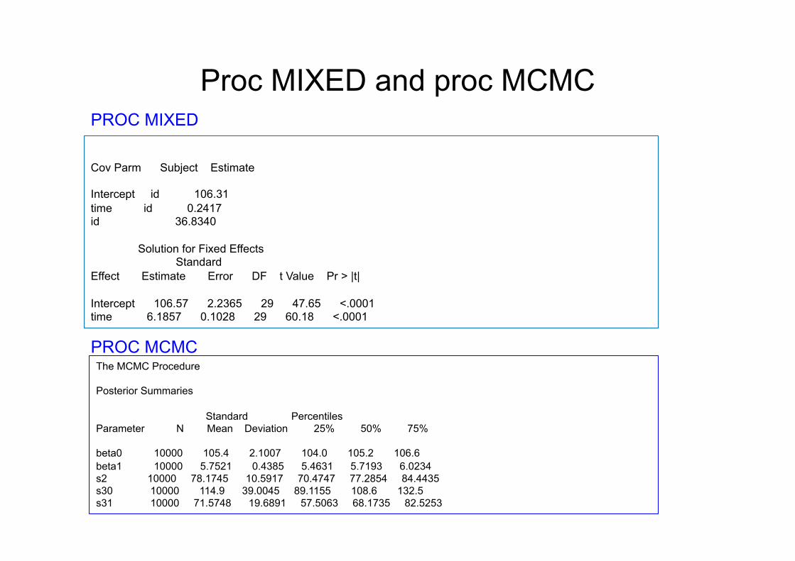
Proc MIXED and proc MCMC
The MCMC Procedure
Posterior Summaries
Standard Percentiles Parameter N Mean Deviation 25% 50% 75%
beta0 10000 105.4 2.1007 104.0 105.2 106.6 beta1 10000 5.7521 0.4385 5.4631 5.7193 6.0234 s2 10000 78.1745 10.5917 70.4747 77.2854 84.4435 s30 10000 114.9 39.0045 89.1155 108.6 132.5 s31 10000 71.5748 19.6891 57.5063 68.1735 82.5253
Cov Parm Subject Estimate
Intercept id 106.31 time id 0.2417 id 36.8340
Solution for Fixed Effects Standard Effect Estimate Error DF t Value Pr > |t|
Intercept 106.57 2.2365 29 47.65 <.0001 time 6.1857 0.1028 29 60.18 <.0001
PROC MIXED
PROC MCMC

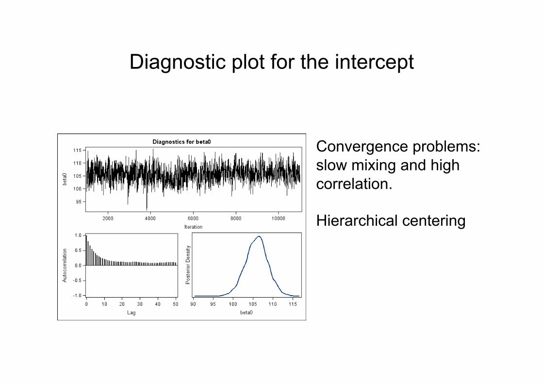
Diagnostic plot for the intercept
Convergence problems: slow mixing and high correlation.
Hierarchical centering.

Hierarchical centering: model formulation
A random intercept and random slope model:
The mean of the “random” effects is not zero but the “fixed” effects.
Prior models for b0i and b1i
Hyperprior models for βs
Hyperprior for the variance components
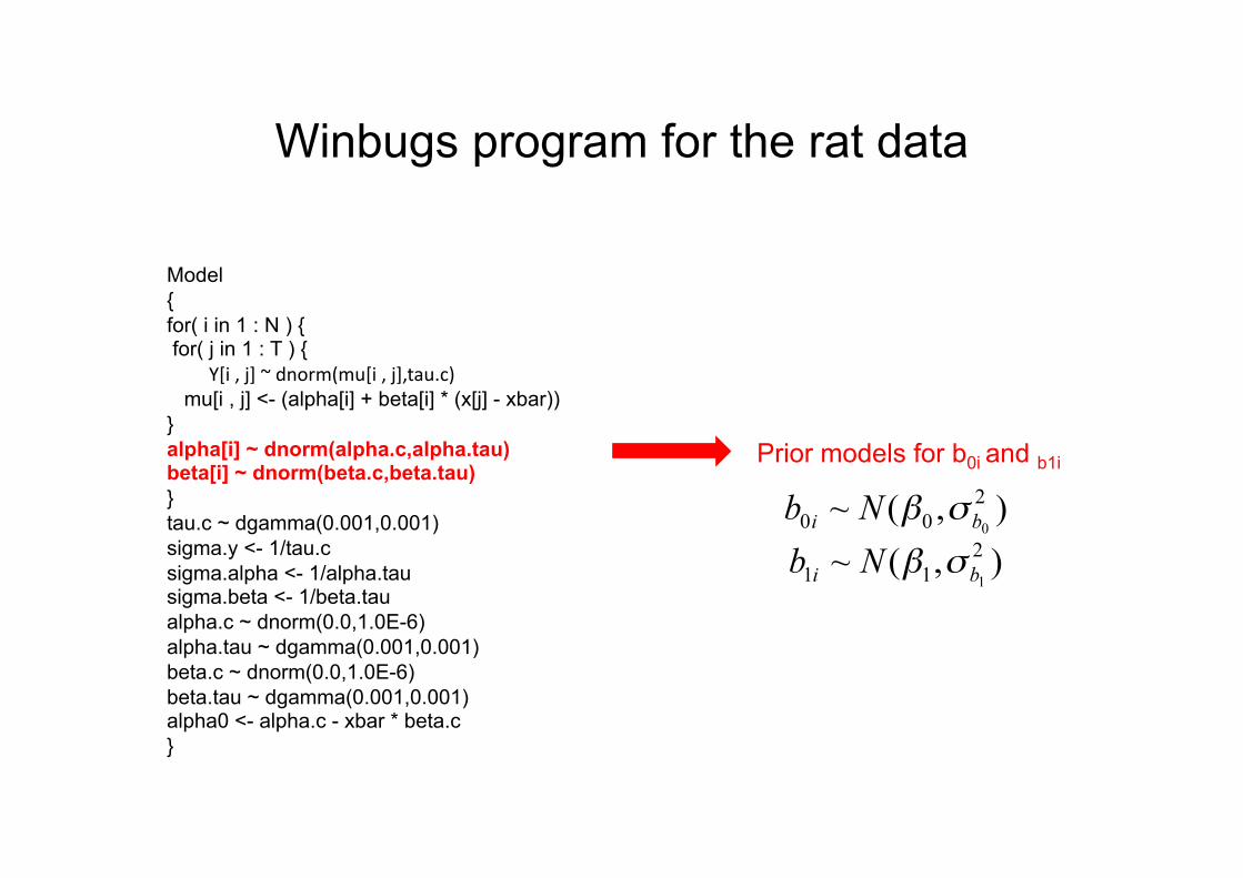
Winbugs program for the rat data
Model { for( i in 1 : N ) { for( j in 1 : T ) { Y[i , j] ~ dnorm(mu[i , j],tau.c) mu[i , j] <- (alpha[i] + beta[i] * (x[j] - xbar)) } alpha[i] ~ dnorm(alpha.c,alpha.tau) beta[i] ~ dnorm(beta.c,beta.tau) } tau.c ~ dgamma(0.001,0.001) sigma.y <- 1/tau.c sigma.alpha <- 1/alpha.tau sigma.beta <- 1/beta.tau alpha.c ~ dnorm(0.0,1.0E-6) alpha.tau ~ dgamma(0.001,0.001) beta.c ~ dnorm(0.0,1.0E-6) beta.tau ~ dgamma(0.001,0.001) alpha0 <- alpha.c - xbar * beta.c }
Prior models for b0i and b1i
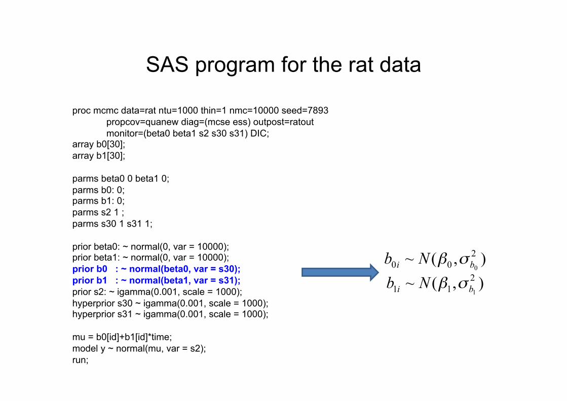
SAS program for the rat data
proc mcmc data=rat ntu=1000 thin=1 nmc=10000 seed=7893 propcov=quanew diag=(mcse ess) outpost=ratout monitor=(beta0 beta1 s2 s30 s31) DIC; array b0[30]; array b1[30];
parms beta0 0 beta1 0; parms b0: 0; parms b1: 0; parms s2 1 ; parms s30 1 s31 1;
prior beta0: ~ normal(0, var = 10000); prior beta1: ~ normal(0, var = 10000); prior b0 : ~ normal(beta0, var = s30); prior b1 : ~ normal(beta1, var = s31); prior s2: ~ igamma(0.001, scale = 1000); hyperprior s30 ~ igamma(0.001, scale = 1000); hyperprior s31 ~ igamma(0.001, scale = 1000);
mu = b0[id]+b1[id]*time; model y ~ normal(mu, var = s2); run;

Winbugs and SAS output
node mean sd MC error 2.5% median 97.5% start sample alpha0 106.5 3.656 0.04112 99.44 106.5 113.8 1000 10001 beta.c 6.185 0.1062 0.0013 5.975 6.185 6.395 1000 10001 Sigma.alpha 219.3 64.82 0.6982 125.0 208.3 372.1 1000 10001 sigma.beta 0.2728 0.09908 0.001621 0.1266 0.2572 0.5129 1000 10001 sigma.y 37.25 5.687 0.09148 27.61 36.73 49.69 1000 10001
The MCMC Procedure
Posterior Summaries
Standard Percentiles Parameter N Mean Deviation 25% 50% 75%
beta0 10000 105.9 2.8147 104.1 106.0 107.7 beta1 10000 6.2014 1.5549 5.1696 6.1859 7.2083 s2 10000 58.1899 7.9568 52.7546 57.3587 63.0212 s30 10000 191.4 64.1846 146.4 179.2 222.6 s31 10000 73.4174 19.7368 59.6083 70.6727 84.4961
Winbugs
SAS
Diagnostic plot for the intercept
Convergence problems: slow mixing and high correlation.
Hierarchical centering

Improving convergence
proc mcmc data=rat nbi=1000 thin=5 nmc=50000 seed=7893…..
We can run the model for higher number of iteration and monitor every k (k=5 in our example) iterations.

Winbugs and SAS output
Standard Percentiles Parameter N Mean Deviation 25% 50% 75%
beta0 10000 106.3 2.9998 104.3 106.3 108.3 beta1 10000 6.1629 1.5786 5.1264 6.1772 7.1907 s2 10000 55.3038 8.3116 49.4731 54.4440 60.1196 s30 10000 223.2 72.8559 172.2 210.8 261.9 s31 10000 73.9487 20.4162 59.2302 70.3625 85.2244
node mean sd MC error 2.5% median 97.5% start sample alpha0 106.5 3.656 0.04112 99.44 106.5 113.8 1000 10001 beta.c 6.185 0.1062 0.0013 5.975 6.185 6.395 1000 10001 Sigma.alpha 219.3 64.82 0.6982 125.0 208.3 372.1 1000 10001 sigma.beta 0.2728 0.09908 0.001621 0.1266 0.2572 0.5129 1000 10001 sigma.y 37.25 5.687 0.09148 27.61 36.73 49.69 1000 10001
Winbugs
SAS

Example 5: A changepoint model

Changepoint models
• The simplest changepoint model assumes that yi ∼ P1(y|θ1), i = 1,2,3,...,k and yi ∼ P2(y|θ2) i = k + 1,k + 2,...,n. • Note that P1 and P2 are assumed to be known, in our
example P1 and P2 are both Poisson.

Changepoint model
• The likelihood for this model is given by
• The model assumes that there is a change in the location (and scale) of y and that the change occurred at k.

The British cool mining disasters data
The British cool mining disasters data by year (1=1851,112=1962).
Number of events by year, over a period of 112 years.

Model formulation
• We assume that the number of events yi is a Poisson random variable.
• In this model, the mean is change from λ1 to λ2 at year k + 1. • k, the year of the change is unknown but we know that 1 < k < 112.

Model formulation
We formulate the following hierarchical model:
• Note that k is assumed to be a random variable which follows a uniform distribution. • This means that we assume that the changepoint can occurs at each year between the first and the last year.
likelihood
Prior (for the mean)
Prior for the changepoint

Winbugs program
model { for( i in 1 : N ) { y[i] ~ dpois(mu[i]) log(mu[i]) <-‐ lambda[J[i]] J[i] <-‐ 1 + step(year[i] -‐ x.change-‐ 0.5) } for( j in 1 : 2 ) { lambda[j] ~ dnorm(0.0,1.0E-‐6) } x.change ~ dunif(1,112) }
Prior for the changepoint
Prior for the mean
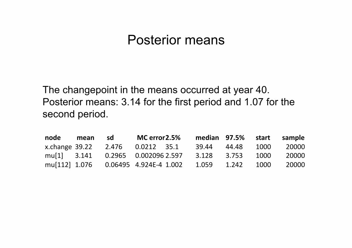
Posterior means
node mean sd MC error 2.5% median 97.5% start sample x.change 39.22 2.476 0.0212 35.1 39.44 44.48 1000 20000 mu[1] 3.141 0.2965 0.002096 2.597 3.128 3.753 1000 20000 mu[112] 1.076 0.06495 4.924E-‐4 1.002 1.059 1.242 1000 20000
The changepoint in the means occurred at year 40. Posterior means: 3.14 for the first period and 1.07 for the second period.

Data, posterior means (for the means) and 95% credible intervals
The change point at month 40

Density estimate for the posterior distribution of the changepoint
The density estimate for the posterior distribution of the changepoint suggests that a more complicated model is needed with possibly two changepoints.
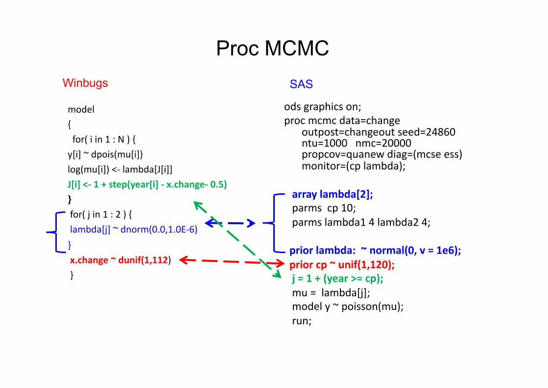
Proc MCMC
ods graphics on; proc mcmc data=change
outpost=changeout seed=24860 ntu=1000 nmc=20000 propcov=quanew diag=(mcse ess) monitor=(cp lambda);
array lambda[2]; parms cp 10; parms lambda1 4 lambda2 4;
prior lambda: ~ normal(0, v = 1e6); prior cp ~ unif(1,120); j = 1 + (year >= cp); mu = lambda[j]; model y ~ poisson(mu); run;
model {
for( i in 1 : N ) {
y[i] ~ dpois(mu[i])
log(mu[i]) <-‐ lambda[J[i]]
J[i] <-‐ 1 + step(year[i] -‐ x.change-‐ 0.5)
}
for( j in 1 : 2 ) {
lambda[j] ~ dnorm(0.0,1.0E-‐6)
}
x.change ~ dunif(1,112)
}
Winbugs SAS
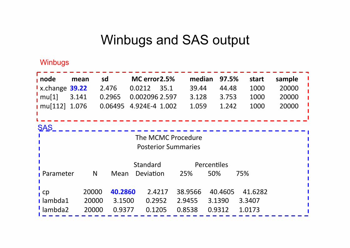
Winbugs and SAS output
The MCMC Procedure Posterior Summaries
Standard Percen,les Parameter N Mean Devia,on 25% 50% 75%
cp 20000 40.2860 2.4217 38.9566 40.4605 41.6282 lambda1 20000 3.1500 0.2952 2.9455 3.1390 3.3407 lambda2 20000 0.9377 0.1205 0.8538 0.9312 1.0173
node mean sd MC error 2.5% median 97.5% start sample x.change 39.22 2.476 0.0212 35.1 39.44 44.48 1000 20000 mu[1] 3.141 0.2965 0.002096 2.597 3.128 3.753 1000 20000 mu[112] 1.076 0.06495 4.924E-‐4 1.002 1.059 1.242 1000 20000
Winbugs
SAS
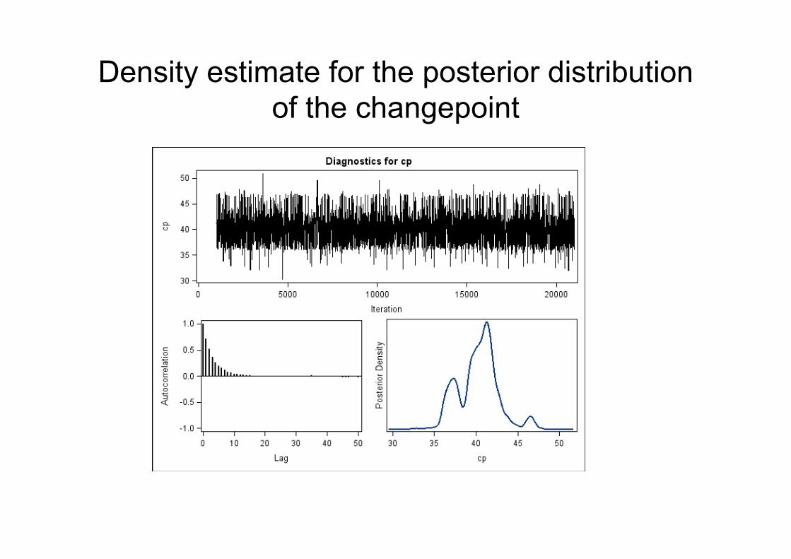
Density estimate for the posterior distribution of the changepoint

Thank you !!!