heterogeneous multi-agent deep reinforcement learning for ... · heterogeneous multi-agent deep...
TRANSCRIPT

Heterogeneous Multi-Agent Deep Reinforcement
Learning for Traffic Lights Control
Jeancarlo Josue Arguello Calvo
A dissertation submitted to University of Dublin, Trinity College
in fulfilment of the requirements for the degree of
Master of Science in Computer Science Future Networked
Systems
August 2018

Declaration
I, the undersigned, declare that this work has not previously been submitted as an
exercise for a degree at this, or any other University, and that unless otherwise stated,
is my own work.
Jeancarlo Josue Arguello Calvo
August 26, 2018
Permission to Lend and/or Copy
I, the undersigned, agree that Trinity College Library may lend or copy this thesis
upon request.
Jeancarlo Josue Arguello Calvo
August 26, 2018

Acknowledgments
To my lovely girlfriend Vivian, for supporting me unconditionally during all this year
that we have been apart. To my supervisor, Prof. Ivana Dusparic, for her guidance in
this research process. To my roommate, Larry, for always being there. And finally, to
all my family for all their support, for believe in me and for always being there for me
without questioning me.
Gracias Totales y Pura vida!!!
Jeancarlo Josue Arguello Calvo
University of Dublin, Trinity College
August 2018
iv

Abstract
People are wasting time in traffic jams that often are caused by an inefficient control
of traffic lights in intersections. In recent years several approaches have been taken in
order to optimize traffic flow in junctions. The most promising technique has been
Reinforcement Learning (RL) due to its capacity to learn the dynamics of complex
problems without any human intervention. Different RL implementations have been
applied in urban traffic control (UTC) to optimize towards single and multiple agents
achieving collaboration. The main problem of these approaches is the curse of dimen-
sionality that arises from the exponential growth of the state and action spaces because
of the number of intersections.
RL had a breakthrough when it was combined with Neural Networks to implement a
method so called Deep Reinforcement Learning (DRL) which enhances hugely the per-
formance of RL for large scale problems. Cutting edge Deep Learning (DL) techniques
have demonstrated to work very well for traffic lights in single agent environments.
Nonetheless, when the problem scales up to multiple intersections the need for coor-
dination becomes more complex, and as a result, the latest studies take advantage of
the similarity of agents in order to train several agents at the same time. However, the
usage of homogeneous junctions is not a real world scenario where a city has different
layouts of intersections.
This thesis proposes to use Independent Deep Q-Network (IDQN) to train hetero-
v
geneous multi-agents to deal with both the curse of dimensionality and the need for
collaboration. The curse of dimensionality is handled by using the Deep Q-Network
technique, whose performance and stability is enhanced by using aggregated methods
such as Dueling Networks for faster training by computing separately the value and
the advantage functions, Double Q-Learning for selecting better Q-values by preventing
overoptimistic value estimations and Prioritized Experience Replay for learning more
efficient from the experience replay memory by sampling more frequently transitions
from which there is a high expected learning progress. IDQN trains simultaneously and
separately each agent which allow us to support heterogeneous agents. Unfortunately,
this technique can lead to convergence problems because one agent’s learning makes
the environment appear non-stationary to other agents, and this problem conflicts with
experience replay memory on which DQN relies. We address this issue by conditioning
each agent’s value function on a fingerprint that disambiguates the age of the data
sampled from the replay memory.
The proposed solution is evaluated in the widely used open source SUMO simula-
tor. We demonstrate that the proposed IDQN technique is suitable for optimization of
traffic light control in a heterogeneous multi-agent setting with the usage of the pro-
posed fingerprint technique that stabilizes the experience replay memory in order to
deal with non-stationary environments. We show that it outperforms normal fixed-time
and DQN without experience replay.
vi

Contents
Acknowledgments iv
Abstract v
List of Tables xi
List of Figures xii
Chapter 1 Introduction 1
1.1 Multi-Agent Training Schemes . . . . . . . . . . . . . . . . . . . . . . . 2
1.1.1 Centralized . . . . . . . . . . . . . . . . . . . . . . . . . . . . . 2
1.1.2 Parameter Sharing . . . . . . . . . . . . . . . . . . . . . . . . . 3
1.1.3 Independent . . . . . . . . . . . . . . . . . . . . . . . . . . . . . 3
1.2 Issues in Multi-Agent Environments . . . . . . . . . . . . . . . . . . . . 4
1.2.1 Agent Dependency . . . . . . . . . . . . . . . . . . . . . . . . . 4
1.2.2 Agent Heterogeneity . . . . . . . . . . . . . . . . . . . . . . . . 5
1.2.3 Cooperation in Heterogeneous Environments . . . . . . . . . . . 5
1.3 Thesis Aims and Objectives . . . . . . . . . . . . . . . . . . . . . . . . 6
1.4 Thesis Assumptions . . . . . . . . . . . . . . . . . . . . . . . . . . . . . 6
1.5 Thesis Contribution . . . . . . . . . . . . . . . . . . . . . . . . . . . . . 7
1.6 Document Structure . . . . . . . . . . . . . . . . . . . . . . . . . . . . 8
Chapter 2 Background and Related Work 9
2.1 Reinforcement Learning . . . . . . . . . . . . . . . . . . . . . . . . . . 9
2.1.1 Q-Learning . . . . . . . . . . . . . . . . . . . . . . . . . . . . . 12
2.2 Deep Learning . . . . . . . . . . . . . . . . . . . . . . . . . . . . . . . . 13
vii

2.2.1 Backpropagation . . . . . . . . . . . . . . . . . . . . . . . . . . 13
2.2.2 Convolutional Neural Networks . . . . . . . . . . . . . . . . . . 14
2.2.3 Optimization Algorithms . . . . . . . . . . . . . . . . . . . . . . 15
2.3 Deep Reinforcement Learning . . . . . . . . . . . . . . . . . . . . . . . 16
2.3.1 Deep Q Networks . . . . . . . . . . . . . . . . . . . . . . . . . . 17
2.3.2 Double DQN . . . . . . . . . . . . . . . . . . . . . . . . . . . . 18
2.3.3 Prioritized Experience Replay . . . . . . . . . . . . . . . . . . . 19
2.3.4 Dueling Network . . . . . . . . . . . . . . . . . . . . . . . . . . 21
2.4 Multi-Agent Reinforcement Learning . . . . . . . . . . . . . . . . . . . 22
2.4.1 Independent DQN . . . . . . . . . . . . . . . . . . . . . . . . . 23
2.4.2 Fingerprints . . . . . . . . . . . . . . . . . . . . . . . . . . . . . 24
2.5 Deep Reinforcement Learning in Traffic Control . . . . . . . . . . . . . 24
2.5.1 Multi-Agent Reinforcement Learning . . . . . . . . . . . . . . . 25
2.5.2 Single Agent Deep Reinforcement Learning . . . . . . . . . . . . 31
2.5.3 Multi-Agent Deep Reinforcement Learning . . . . . . . . . . . . 38
2.6 Summary . . . . . . . . . . . . . . . . . . . . . . . . . . . . . . . . . . 43
Chapter 3 Design 44
3.1 Traffic Light Control Problem . . . . . . . . . . . . . . . . . . . . . . . 44
3.1.1 State Representation . . . . . . . . . . . . . . . . . . . . . . . . 45
3.1.2 Action Space . . . . . . . . . . . . . . . . . . . . . . . . . . . . 46
3.1.3 Reward Function . . . . . . . . . . . . . . . . . . . . . . . . . . 49
3.2 Deep Reinforcement Learning Techniques . . . . . . . . . . . . . . . . . 51
3.3 Deep Neural Network Architecture . . . . . . . . . . . . . . . . . . . . 57
3.4 Single Agent Training . . . . . . . . . . . . . . . . . . . . . . . . . . . . 58
3.5 Multi-Agent Design . . . . . . . . . . . . . . . . . . . . . . . . . . . . . 58
3.5.1 Training . . . . . . . . . . . . . . . . . . . . . . . . . . . . . . . 61
3.6 Summary . . . . . . . . . . . . . . . . . . . . . . . . . . . . . . . . . . 61
Chapter 4 Implementation 64
4.1 Simulation Environment . . . . . . . . . . . . . . . . . . . . . . . . . . 64
4.2 Deep Reinforcement Learning . . . . . . . . . . . . . . . . . . . . . . . 65
4.2.1 TrafficEnv . . . . . . . . . . . . . . . . . . . . . . . . . . . . . . 65
viii

4.2.2 TrafficTfInput . . . . . . . . . . . . . . . . . . . . . . . . . . . . 66
4.2.3 DQNAgent . . . . . . . . . . . . . . . . . . . . . . . . . . . . . 66
4.3 Neural Network Architecture . . . . . . . . . . . . . . . . . . . . . . . . 67
4.3.1 Optimizer . . . . . . . . . . . . . . . . . . . . . . . . . . . . . . 70
4.4 Multi-Agent Deep Reinforcement Learning . . . . . . . . . . . . . . . . 72
4.4.1 TrafficEnv . . . . . . . . . . . . . . . . . . . . . . . . . . . . . . 72
4.4.2 DQNAgent . . . . . . . . . . . . . . . . . . . . . . . . . . . . . 73
4.5 IDQN Neural Network . . . . . . . . . . . . . . . . . . . . . . . . . . . 73
4.6 Summary . . . . . . . . . . . . . . . . . . . . . . . . . . . . . . . . . . 74
Chapter 5 Evaluation 75
5.1 Objectives . . . . . . . . . . . . . . . . . . . . . . . . . . . . . . . . . . 75
5.2 Metrics . . . . . . . . . . . . . . . . . . . . . . . . . . . . . . . . . . . . 76
5.3 Evaluation Scenarios . . . . . . . . . . . . . . . . . . . . . . . . . . . . 76
5.3.1 Evaluation Techniques . . . . . . . . . . . . . . . . . . . . . . . 76
5.3.2 Scenarios . . . . . . . . . . . . . . . . . . . . . . . . . . . . . . 77
5.4 Setup . . . . . . . . . . . . . . . . . . . . . . . . . . . . . . . . . . . . . 77
5.4.1 Network Layout . . . . . . . . . . . . . . . . . . . . . . . . . . . 78
5.4.2 Traffic Demand . . . . . . . . . . . . . . . . . . . . . . . . . . . 79
5.4.3 Hyper-paraments . . . . . . . . . . . . . . . . . . . . . . . . . . 80
5.5 Results and Analysis . . . . . . . . . . . . . . . . . . . . . . . . . . . . 80
5.5.1 Low Traffic Load . . . . . . . . . . . . . . . . . . . . . . . . . . 81
5.5.2 High Traffic Load . . . . . . . . . . . . . . . . . . . . . . . . . . 86
5.6 Evaluation Summary . . . . . . . . . . . . . . . . . . . . . . . . . . . . 88
Chapter 6 Conclusions and Future Work 89
6.1 Thesis Contribution . . . . . . . . . . . . . . . . . . . . . . . . . . . . . 89
6.2 Future Work . . . . . . . . . . . . . . . . . . . . . . . . . . . . . . . . . 90
Appendix A Appendix 93
A.1 Traffic Demand Generation . . . . . . . . . . . . . . . . . . . . . . . . . 93
A.2 Metrics for Experiments . . . . . . . . . . . . . . . . . . . . . . . . . . 95
A.3 Complete views of the Implementation of the Deep Neural Network . . 96
ix

Bibliography 99
x
List of Tables
2.1 Existing research in Multi-Agent Reinforcement Learning for Traffic Sig-
nal Control . . . . . . . . . . . . . . . . . . . . . . . . . . . . . . . . . 26
2.2 Test environments of existing research in Multi-Agent Reinforcement
Learning for Traffic Signal Control . . . . . . . . . . . . . . . . . . . . 31
2.3 Existing research in Single Agent Deep Reinforcement Learning for Traf-
fic Signal Control . . . . . . . . . . . . . . . . . . . . . . . . . . . . . . 32
2.4 Existing research in Multi-agent Deep Reinforcement Learning for Traf-
fic Signal Control . . . . . . . . . . . . . . . . . . . . . . . . . . . . . . 39
2.5 Test environments of existing research in Multi-agent Deep Reinforce-
ment Learning for Traffic Signal Control . . . . . . . . . . . . . . . . . 42
3.1 DRL techniques evaluation hyper-parameters . . . . . . . . . . . . . . . 50
3.2 DRL techniques evaluation hyper-parameters . . . . . . . . . . . . . . . 51
4.1 Reward function evaluation hyper-parameters . . . . . . . . . . . . . . 70
5.1 Multi-agent evaluation hyper-parameters . . . . . . . . . . . . . . . . . 81
xi

List of Figures
1.1 Heteregenous Muti-agent setting . . . . . . . . . . . . . . . . . . . . . . 4
2.1 Reinforcement Learning [1] . . . . . . . . . . . . . . . . . . . . . . . . . 11
2.2 A popular single stream Q-network (top) and the dueling Q-network
(bottom). The dueling network has two streams to separately estimate
(scalar) state-value and the advantages for each action; the green output
module implements equation (2.21) to combine them. Both networks
output Q-values for each action [2] . . . . . . . . . . . . . . . . . . . . 22
2.3 Distributed W-Learning [3] . . . . . . . . . . . . . . . . . . . . . . . . . 27
2.4 Architecture [4] . . . . . . . . . . . . . . . . . . . . . . . . . . . . . . . 28
2.5 The deep SAE neural network for approximating Q function [5] . . . . 33
2.6 DNN structure. Note that the small matrices and vectors in this figure
are for illustration simplicity, whose dimensions should be set accord-
ingly in DNN implementation [6] . . . . . . . . . . . . . . . . . . . . . 34
2.7 Agent training process [6] . . . . . . . . . . . . . . . . . . . . . . . . . 35
2.8 The architecture of the deep convolutional neural network to approxi-
mate the Q-value [7] . . . . . . . . . . . . . . . . . . . . . . . . . . . . 36
2.9 The architecture of the reinforcement learning model in our system [7] . 37
2.10 Non parametric control learnt by experience. A neural network decides [8] 40
3.1 State Representations . . . . . . . . . . . . . . . . . . . . . . . . . . . . 45
3.2 Traffic light phases available to agent with 4 roads . . . . . . . . . . . . 47
3.3 Traffic light phases available to agent with 3 roads . . . . . . . . . . . . 48
3.4 Reward Functions Experiment . . . . . . . . . . . . . . . . . . . . . . . 50
3.5 DQN Single Agent Experiments . . . . . . . . . . . . . . . . . . . . . . 52
xii

3.6 DDQN Single Agent Experiments . . . . . . . . . . . . . . . . . . . . . 53
3.7 Prioritized DDQN Single Agent Experiments . . . . . . . . . . . . . . . 55
3.8 Prioritized Dueling DDQN Single Agent Experiments . . . . . . . . . . 56
3.9 The architecture of the Deep Neural Network. . . . . . . . . . . . . . . 57
3.10 Multi-Agent Partial Observation . . . . . . . . . . . . . . . . . . . . . . 61
4.1 DRL Traffic Control System Class Diagram . . . . . . . . . . . . . . . 65
4.2 Dueling Network built with TensorFlow [9] . . . . . . . . . . . . . . . . 68
4.3 Deep Q-Networks built with TensorFlow [9] . . . . . . . . . . . . . . . 69
4.4 Comparison between RMSProp and Adam Optimizers . . . . . . . . . . 71
4.5 IDQN Traffic Control System Class Diagram . . . . . . . . . . . . . . . 72
4.6 Independent Deep Q-Networks for 3 agents built with TensorFlow [9] . 73
5.1 Network Layout for Multi-Agent Experiments . . . . . . . . . . . . . . 78
5.2 Entry and Departure points in Network for Multi-Agent Experiments.
Green points correspond to entry and departure points, while blue points
are intersections. . . . . . . . . . . . . . . . . . . . . . . . . . . . . . . 79
5.3 Low Traffic IDQN Experiments . . . . . . . . . . . . . . . . . . . . . . 83
5.4 Low Traffic IDQN Experiments with Standard ERM . . . . . . . . . . 85
5.5 High Traffic IDQN Experiments . . . . . . . . . . . . . . . . . . . . . . 87
A.1 Single intersection routes . . . . . . . . . . . . . . . . . . . . . . . . . . 94
A.2 Whole view of the Neural Network Architecture built with TensorFlow [9] 96
A.3 Zoomed upper view of Whole Neural Network Architecture built with
TensorFlow [9] . . . . . . . . . . . . . . . . . . . . . . . . . . . . . . . . 97
A.4 Zoomed lower view of Whole Neural Network Architecture built with
TensorFlow [9] . . . . . . . . . . . . . . . . . . . . . . . . . . . . . . . . 98
xiii

Chapter 1
Introduction
This thesis addresses heterogeneous multi-agents for urban traffic control (UTC) sys-
tems as the first study applying Deep Reinforcement Leaning (DRL) in a heterogeneous
network layout which is a reflection of the cities in the real world. It proposes the usage
of DRL to deal with the curse of dimensionality that suffers Reinforcement Learning
approaches by using Neural Networks which works better for complex large problems.
It also uses Indepedent Q-Learning (IQL), where each agent learns independently and
simultaneously its own policy, treating other agents as part of the environment. How-
ever, the environment becomes nonstationary from the point of view of each agent, as
it involves the interaction with other agents who are themselves learning at the same
time, ruling out any convergence guarantees. The technique used for this problem is
Deep Q-Networks which relies in a component so called experience replay memory in
order to stabilize and improve the learning. However, this memory is incompatible
with non-stationary environments. In order to combine the experience replay memory
and IQL, we used a technique of fingerprinting which stabilizes the memory against
the non-stationarity. This fingerprint disambiguates the age of the data sampled from
the replay memory. We evaluate the usage of IQL with Deep Q-Networks in a multi-
agent setting by using a simulation of an urban traffic control system. This chapter
motivates the work, introduces multi-agent optimization and IQL, outlines the main
contributions of this work, and presents a roadmap for the remainder of the thesis.
1

1.1 Multi-Agent Training Schemes
This section describes three training schemes for multi-agent DRL. It outlines the
advantages and disadvantages of each approach, and describes how each can be used
in DRL.
The following approaches to multi-agent decision making under uncertainty are
based in the theory of Markov Decision Processes (MDPs), for example Decentralized
Partially Observable MDPs (Dec-POMDPs) [10] which are intractable without commu-
nication; and Multiagent MDPs (MMDPs) and POMDPs (MPOMDPs), which assume
free communication between agents [11].
1.1.1 Centralized
This method assumes a joint model for the actions and observations of all the agents.
A centralized policy maps the joint observation of all the agents to a joint action, which
is based on a MPOMDP policy. The major problem of a MPOMDP is the exponential
growth in the observation and actions spaces with the number of agents. This can be
address by factoring the action space of centralized multi-agent systems. Assuming
that the joint action space can be split into individual components for each agent, the
factored centralized multi-agent system can then be defined as a set of independent
sub-policies that map the joint observation to an action for a single agent [12].
In a policy gradient approach this is done by dividing the joint action probability
as P(−→a ) =∏
i P(ai) where ai are the individual actions of an agent. As a result,
the output of the neural network policy has to capture just the action distributions
for each single agent rather than the joint action distributions for all the agents. In
systems with discrete actions, the size of the action space is decreased from ‖A‖n to
n‖A‖, where n is the number of agents and A is the action space for a individual agent.
In spite of the significant reduction in the size of the action space, the exponential
growth in the observation space makes centralized approaches unusable for complex
cooperative problems [12].
2

1.1.2 Parameter Sharing
This approach is only suitable for homogeneous agents, hence it is inappropriate for the
goal of this research which aims to work with heterogeneous agents. When the agents
are homogeneous, their policies can be trained more efficiently using parameter shar-
ing. In this method all the agents share the parameters of a single policy. This allows
the policy to be trained with the experiences of all agents at the same time. Nonethe-
less, it allows different behaviors between agents because each agent receives different
observations. In this approach, the control is decentralized but not the learning, which
makes it the most scalable approach out of the three described in this section, however
its disadvantage is that it does not work for heterogeneous agents [12].
A policy gradient version of the parameter sharing training approach is presented
in [13]. At each iteration of the TRPO algorithm, the decentralized policy is used to
sample trajectories from each agent. The batch of trajectories from all the agents is
used to compute the advantage value and maximize the following objective [12].
1.1.3 Independent
In this method each agent learns its own policy by following a Dec-POMDP approach.
Independent policies map an agents local observation to an action for that agent.
One strength is that it makes learning of heterogeneous policies easier. This can be
advantageous in situations where agents may need to take on specific roles in order to
coordinate and receive reward. Although, there are two complications on this approach.
First, the training of independents policies does not scale to large numbers of agents
because the agents do not share experience with each other. The training requires a
policy for each agent, which increases the computational and memory resources needed
when the policies are represented by complex models such as neural networks. Second,
as the agents are learning and adjusting their policies simultaneously, the modifications
in the policies make the environment dynamics non-stationary. This normally leads
to instability issues, and it is incompatible with DRL approaches based on Deep Q-
Networks (DQN) that relies on experience replay memory to stabilize and enhance the
learning. The standard experience replay memory of DQN can quickly turns the stored
experiences obsolete due to the updates of other agents that are perceived as part of
the environment [12]. We address the latter issue by using a fingerprint as proposed in
3
[14]. This technique is going to be explained later in Chapter 2 and 4.
1.2 Issues in Multi-Agent Environments
In this section we introduce and analyze properties of multi-agent that can conflict to
achieve a good performance of the UTC system. Specifically, we discuss issues of agent
heterogeneity dependency, as well as consequences that these might have on agent
collaboration.
1.2.1 Agent Dependency
The performance of an agent in a multi-agent settings can be impacted, directly or
indirectly, and both positively and negatively, by other agents actions [15]. In the case
of a UTC system the performance of one junction can be affected by some or all of its
upstream and/or downstream neighbours.
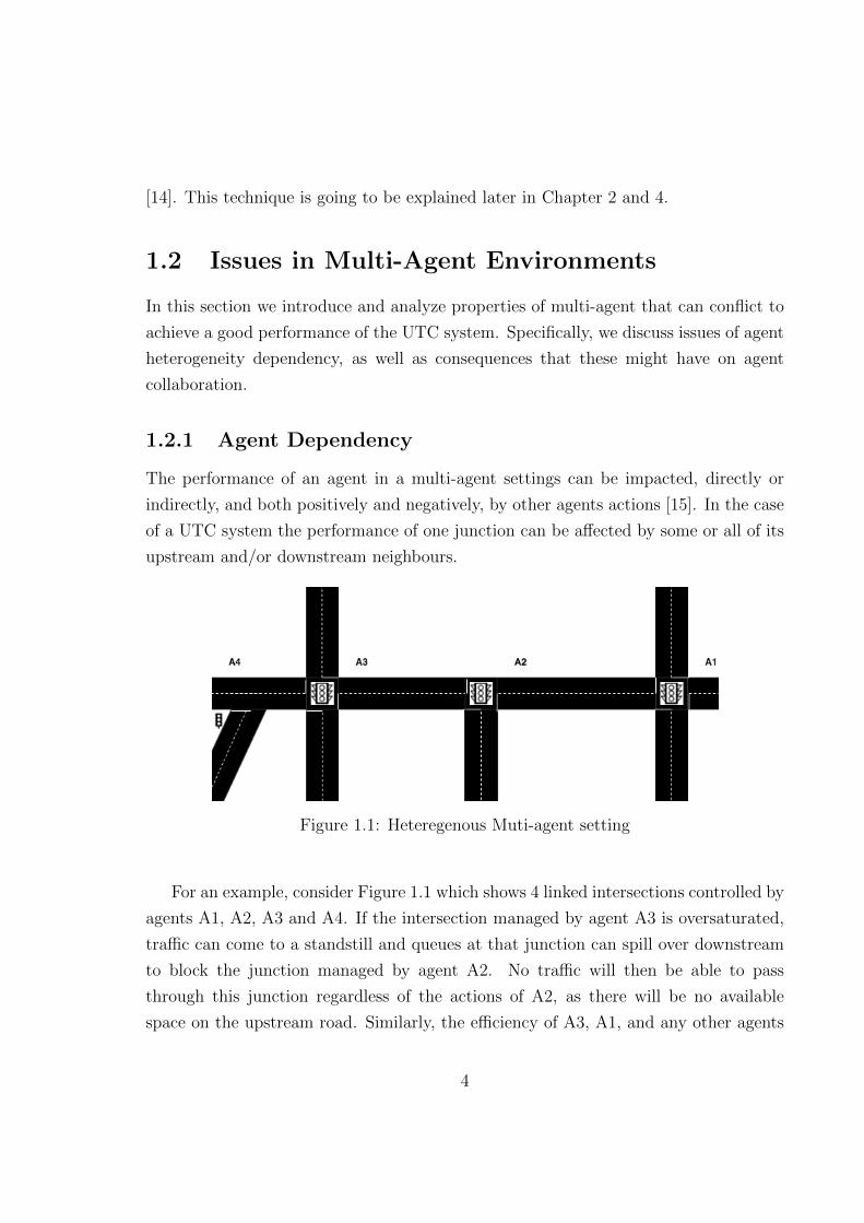
Figure 1.1: Heteregenous Muti-agent setting
For an example, consider Figure 1.1 which shows 4 linked intersections controlled by
agents A1, A2, A3 and A4. If the intersection managed by agent A3 is oversaturated,
traffic can come to a standstill and queues at that junction can spill over downstream
to block the junction managed by agent A2. No traffic will then be able to pass
through this junction regardless of the actions of A2, as there will be no available
space on the upstream road. Similarly, the efficiency of A3, A1, and any other agents
4

at other intersections that feed traffic to A2 can cause oversaturation at A2 if they are
letting pass more traffic than A2 is clearing. The dependency can also be extended
to the agents further downstream from A2, such as A4, as that agent influences the
performance of A3, which in turn influences the performance of A2, causing a potential
dependency between non neighbouring agents A2 and A4. As a consequence, there is
a transitive dependency between all of the agents in a UTC system. Due to this
dependency, agents should consider not only their local view benefit, but also the
repercussion of other agents’ actions, specially their immediate neighbours.
1.2.2 Agent Heterogeneity
It is specially hard for agents to take the needs of other agents into consideration when
agents are heterogeneous and implement different policies. The first source of hetero-
geneity is the discrepancy in the agents operating environment and capabilities. For
instance, in a UTC system the intersections can have several layouts, i.e., the number
of incoming and outgoing ways and the allowed traffic operations can be distinct. In
RL, this results on agents having different state and action spaces, since the combi-
nations of traffic signal phases available to agents managing the junctions of different
layout differ. As a consequence, the agents do not have a common interpretation of
the meaning of particular states and/or actions.
1.2.3 Cooperation in Heterogeneous Environments
Due to the aforementioned issues, an optimal performance of the system as a whole
might not be as simple as optimizing the performance of all agents individually, but
they may require to cooperate with each other in order to achieve a global optimal
behaviour. In order to implement cooperation, some information should be shared
or exchange with the purpose of overcoming the aforementioned problems. However,
heterogeneous agents are not able to exchange experiences with each other, as their
state and actions spaces differ, such that the learning obtained at one agent is not
useful to other agents with different state-action spaces. Once the exchange information
component is chosen, it is important to determine with whom each agent is going to
cooperate. As the levels of dependency between agents might differ, an agent might
only need to collaborate with other agents whose actions it is influenced by, and agents
5

that are influenced by its local actions. For example, it might need to cooperate only
with neighbour agents.
1.3 Thesis Aims and Objectives
The general objective of the thesis is to address the gap in DRL-based self-optimization
techniques for traffic control lights, whereby existing techniques address either a sin-
gle agent, or address collaborative optimization in multi-agent systems, but towards
only homogeneous agents. We believe that, if DRL-based techniques are widely used
for optimization in UTC systems, they need to be able to optimize towards multiple
heterogeneous agents simultaneously. Such an approach can be applied to realistic
intersection scenarios of any city worldwide. This thesis argues that DRL is a suitable
basis for such a technique, due its ability to learn suitable behaviours without requiring
a model of the environment, and ability to deal with large complex problems. This
thesis analyses requirements for such an multi-agent DRL-based method for optimiza-
tion heterogeneous environments, presents the design and implementation of a suitable
technique, and evaluates it in a simulation of UTC.
1.4 Thesis Assumptions
In designing and evaluating this multi-agent DRL, this thesis makes a number of as-
sumptions about the environment in which it is to be deployed. The design assumptions
limit the scope of the thesis by limiting the number of issues that it addresses, while the
evaluation environment assumptions are imposed by the capabilities and limitations of
the UTC simulation system used.
In this thesis, agents are assumed to be stationary, i.e., their locations are fixed and
they do not move through the environment. This is the case in our evaluation area, as
agents are associated with traffic lights, which are stationary. Agents are also assumed
to be failure-free, and hence issues arising from agents not being able to contact their
neighbours, or agents receiving incomplete or inaccurate information are not addressed.
The state space is assumed to be a post-processing representation of video images
of traffic cameras, additionally is assumed that all the intersections have the same
6

capabilities of observation of the state, i.e., the same viewpoint, image resolution and
view size.
System timing on all agents in the system is synchronized, and the agents are
assumed to make decisions simultaneously at fixed time intervals. This thesis does
not investigate how asynchronous decision making would impact on the design and
performance of the multi-agent DRL approach.
In the simulations performed in this thesis, the behaviour of traffic lights is de-
termined by the simulated control mechanism (DRL or the baselines), while the be-
haviour of cars, i.e., their starting position, route, and destination, are predefined. A
consequence of this characteristic of the simulation environment is that, if there is no
available road space for cars to join the simulation at the junction specified as their
starting position, they are not inserted into the simulation.
1.5 Thesis Contribution
This thesis identifies and motivates the need for a DRL-based heterogeneous multi-
agent technique as it has not been studied before. It intends to answer the question
of if DRL is a suitable technique for heterogeneous multi-agent for UTC system. It
presents the challenges of a heterogeneous multi-agent UTC system using DRL, and
based on them proposes the requirements for such a technique. The main contri-
bution of the thesis is the design, implementation and evaluation of a DRL method
for heterogeneous multi-agent traffic light control system. Unlike existing DRL-based
techniques, Independent Deep Q-Network (IDQN) enables the optimization of hetero-
geneous junctions that are a more realistic reflection of real cities where the layout of
the intersections are different. IDQN enables collaboration between agents regardless
of the policies they implement, enabling optimization in heterogeneous environments.
IDQN uses Independent Q-Learning where each agent independently learns its own
policy, treating other agents as part of the environment. IDQN learns and takes into
consideration the dependencies between policies of other agents in order to improve
their local and global performance with the usage of a fingerprint in the experience
replay memory that avoids the instability caused by the non-stationarity of the en-
vironment. Finally, this thesis evaluates the technique in a simulation of UTC. The
evaluation shows that it is suitable for application in UTC, as it outperforms existing
7

UTC techniques.
1.6 Document Structure
The structure of the thesis is as follows. Chapter 2 presents the background material
about the cutting edge Reinforcement Learning and Deep Learning techniques that
are used for the proposed work. It focuses on RL model free algorithms, providing
the background of these techniques. It also presents the state-of-the-art studies in the
field for single and multi-agent environments with and without Deep Learning for UTC
systems. It introduces multi-agents methods for UTC and different Neural Networks
architectures for single and multi-agent systems. Chapter 3 describes the design of
the proposed research. Chapter 4 describes the implementation of the design stated in
Chapter 3. Chapter 5 presents the evaluation of the suggested study as a heterogeneous
multi-agent DRL technique and analyses the findings. Chapter 6 concludes this thesis
with the summary of the work and outlines the issues that remain open for future work.
8
Chapter 2
Background and Related Work
This sections covers the main technical concepts to be used in order to build an adaptive
traffic signal control (ATSC). The first section presents Reinforcement Learning which
is essential for dynamic complex problems and its most popular technique, so called Q-
Learning. The second section introduces the concept of Deep Learning and its impact
nowadays. The third sections describes Deep Reinforcement Learning and the state-
of-the-art methods for Deep Q-Learning. The next section describes our proposed
technique, Independent Deep Q-Network (IDQN) with fingerprint. The last section
gives the reasons to use DRL in UTC problems and it presents recent studies for single
and multi agents in UTC problems.
2.1 Reinforcement Learning
Reinforcement learning (RL) is about learning optimal actions from specific situations
where the agent has to discover which actions maximize a reward signal by explor-
ing them in a trial-and-error basis. These actions may affect future situations and
subsequent reward signals [1].
RL is formulated in the mathematical representation of a complex decision making
process called Markov Decision Process (MDP) [16], which it is defined by:
• A time step t.
• A set of states s ∈ S.
9

• A set of actions a ∈ A.
• A transition function T(st, at, st+1), which is the probability that an action a
leads to st+1 from st, i.e. P(st+1 | st, at).
• A reward function R(st, at, st+1).
RL is the optimal control of incompletely-known MDP where the transition and the
reward functions are unknown. They are learned during the RL training. Therefore, in
RL an active decision making agent interacts with the environment in order to achieve
a goal regardless of the uncertainty.
Beyond the agent and the environment, there are other four subcomponents: (1) a
policy, (2) a reward signal, (3) a value function and (4) the model of the environment.
Firstly, a policy defines the behaviour of the agent at a given time, more specifically, a
policy maps observed states of the environment to actions in order to be taken when
in those states. In RL, the agent seeks to learn the optimal policy that corresponds
to the best action for every possible state, i.e. π* : S → A, where π represents the
policy. Secondly, a reward signal defines the goal in a RL system. On each time
step, the environment sends a reward to the agent when it transitions from a state st
to a state st+1. The agent’s objective is to maximize the expected reward, therefore
the policy will be altered in order to achieve the optimal policy that accomplishes
this. Thirdly, the value function is associated to a state, and it indicates the total
amount of reward an agent can expect to acquire over the long term, starting from
that state s and by following the policy π. Finally, the model mimics the dynamics of
the environment (transition and reward functions) allowing to make inferences about
how the environment will behave. Models are used for planning, meaning that the
agent can decide which actions to take by considering possible future situations before
it had experienced them. The algorithms that use models and planning are called
model-based. On the other hand, the algorithms that rely on trial-and-error to update
its knowledge are called model-free. Model-based algorithms are impractical as the
space and action spaces grows, therefore for complex problems model-free algorithms
are utilized, and are the ones that are going to be discussed further in this research.
Given these points, RL is a system where an agent interacts with the environment.
On each time step t, the agent perceives an state st in state space S from where it
10
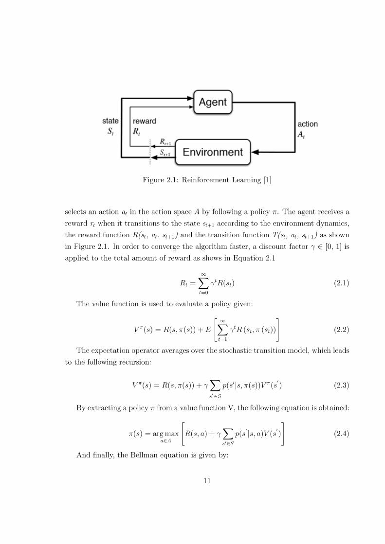
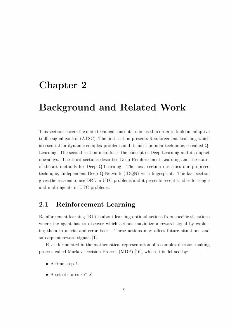
Figure 2.1: Reinforcement Learning [1]
selects an action at in the action space A by following a policy π. The agent receives a
reward rt when it transitions to the state st+1 according to the environment dynamics,
the reward function R(st, at, st+1) and the transition function T(st, at, st+1) as shown
in Figure 2.1. In order to converge the algorithm faster, a discount factor γ ∈ [0, 1] is
applied to the total amount of reward as shows in Equation 2.1
Rt =∞∑t=0
γtR(st) (2.1)
The value function is used to evaluate a policy given:
V π(s) = R(s, π(s)) + E
[∞∑t=1
γtR (st, π (st))
](2.2)
The expectation operator averages over the stochastic transition model, which leads
to the following recursion:
V π(s) = R(s, π(s)) + γ∑s′∈S
p(s′|s, π(s))V π(s′) (2.3)
By extracting a policy π from a value function V, the following equation is obtained:
π(s) = arg maxa∈A
[R(s, a) + γ
∑s′∈S
p(s′ |s, a)V (s
′)
](2.4)
And finally, the Bellman equation is given by:
11

V ∗(s) = maxa∈A
[R(s, a) + γ
∑s′∈S
p(s′|s, a)V ∗(s
′)
](2.5)
Solving this non-linear system of equations for each state s yields the optimal value
function, and consequently an optimal policy π*.
2.1.1 Q-Learning
As in RL, the transition and the reward functions are unknown because it has no prior
knowledge of the model (model-free), RL agents learn Q-values instead of learning
values. A Q-value is a function of state-action pair that returns a real value: Q: S x A
→ R. By using Q-values, the policy can be represented as:
π(s) = arg maxa∈A
Q(s, a) (2.6)
where the Q-value can be learned by using Q-learning updates [17]:
Q(s, a) = (1− α)Q(s, a) + α[R(s, a) + maxa∈A
Q(s′, a′)] (2.7)
where 0 < α ≤ 1 is a learning rate.
[17] demonstrated that Q-learning converges to the optimal policy with probability
1 as long as all actions are repeatedly sampled in all states and the Q-values are
represented discretely. Exploration is needed to make sure all action in all states are
sampled. As a consequence the dilemma of the trade-off between exploration and
exploitation arises. An agent must prefer the actions that it has found produce highest
rewards given actions it has tried in the past. However, in order to discover those
actions, it has to try new actions (exploration) that it has not performed before. At
some point, the agent has to use what it has learned (exploitation) in order to get
rewards. One common technique for exploration is to randomly select actions with
small probability, this is known as ε-greedy exploration.
12

2.2 Deep Learning
Deep learning (DL) is an machine learning implementation that is based in the knowl-
edge of the human brain, specifically in the biological neural networks, statistics and
applied math. In the last years, deep learning has had a huge growth and impact on its
popularity and usefulness, mainly due to the development of more powerful computers,
larger datasets and better techniques to train deeper networks [18].
Computational models that contains multiple processing layers can learn represen-
tations of data by using multiple levels of abstraction called artificial neural networks.
These layers are used by DL representation-learning methods that are obtained by
non-linear modules that each transforms one level of abstraction, from the beginning
with raw input to a higher abstract level. The main aspect of DL is that these layers
are not built by human, but they are learned directly from the data using a learning
mechanism. A DL architecture is a multilayer stack of simple modules which are sub-
ject to learning and many of them compute non-linear input-output mappings. Each
one of these modules can transform its input to boost both the selectivity and the
invariance of the representation[19].
DL can identify complex structures in large data sets by using the backpropagation
algorithm to indicate changes of internal parameters that are used as part of the pro-
cessing of the representation in each layer basing on the representation in the previous
layer. Deep convolutional nets have brought advances in images, video, speech and
audio recognition, whereas recurrent nets have shined on sequential data such as text
and speech
2.2.1 Backpropagation
The multilayer architectures can be trained by stochastic gradient descent as long as
the modules are relatively smooth functions of their inputs and of their internal weights
by using the backpropagation procedure which is a practical application of the chain
rule of derivatives. The reason is that the derivative of the objective function with
respect to the input of a module can be computed backwards from the gradient with
respect to the output of that module or the input of the subsequent module. The
backpropagation equation can be applied over and over again to spread gradients to
all modules, starting from the output where the prediction is made, until where the
13

input is fed. Once these gradients have been computed, the gradients with respect to
the weights of each module can be computed easier [19].
Another approach is to use feedforward neural network architectures, which can
learn to map a fixed-size to a fixed-size output. A set of units compute a weighted
sum of their inputs from the previous layer and pass the result through a non-linear
function in order to the next layer. The most common used non-linear function is the
rectified linear unit (ReLU). The units that are not in the input or output layer are
so-called hidden units. The hidden layers deceives the input in a non-linear manner
such that the categories become linearly separable by the last layer. Convolutional
neural network (CNN) is a specific feedforward network that is easier to train and it
generalizes better than networks with full connectivity[19].
2.2.2 Convolutional Neural Networks
Convolutional Neural Networks (CNN) processes data fed as multiple arrays. CNNs
are based on four insights: (1) local connections, (2) shared weights, (3) pooling and
the (4) use of many layers.
A CNN is structured as a succession of phases. The first phase consists of two
types of layers: (1) convolutional and (2) pooling layers. The units in a convolutional
layer are arranged in feature maps. Each unit is connected to local patches in the
feature maps of the previous layer through a set of weights called a filter bank, which
is shared for all the units in the respective feature map The result of this local weighted
sum is passed through a non-linearity function. The name of CNN is derived of the
filtering operation carried out by a feature map which is, mathematically, a discrete
convolution. On the other hand, a pooling layer merges semantically similar features
into one. A pooling unit computes the maximum of a local patch of units in one or in
a few feature maps. Adjacent pooling units take input from patches that are shifted
by more than one row or column, thereby reducing the dimension of the representation
and creating an invariance to small shifts and distortions. Backpropagation in CNN is
simple as a regular deep network, allowing all the weights in all the filter banks to be
trained[19].
14
2.2.3 Optimization Algorithms
Gradient descent is the most used algorithm to optimize neural networks. Gradient
descent is a way to minimize the cost function J(θ) by updating the parameters in
the opposite direction of the gradient of the cost function ∇θJ(θ). The most used
algorithms in Deep Learning are: (1) Momentum, (2) Adagrad, (3) AdaDelta, (4)
RMSProp and (5) ADAM.
Adagrad
[20] proposed Adagrad which as a method which adaptively updates parameters based
on a sum of squared gradients per parameter. It uses that value to normalize the
learning rate before the update for each parameter i with the formula:
Gti = Gt−1
i +
(δJ(θ)
δσjt−1
)2
(2.8)
σjt = σjt−1 − α
Gti + ε
+δJ(θ)σδσjt−1
(2.9)
where ε is a small constant to prevent division by zero.
The learning rate for each parameter is set adaptively based on past updates. If
past gradients for parameter i were large, the learning rate for i is small and vice-versa.
By dividing the learning rate by the sum of past square gradients, Adagrad removes
the need for extensive learning rate tuning.
RMSProp
RMSprop and Adadelta have both been developed independently from the need to solve
Adagrads aggressive diminishing learning rates. [21] proposed RMSProp in order to
solve that problem by defining an exponentially decaying average of squared gradients.
Gti = γGt−1
i + (1− γ)
(δJ(θ)
δσjt
)2
(2.10)
where γ is recommended to be 0.9.
15
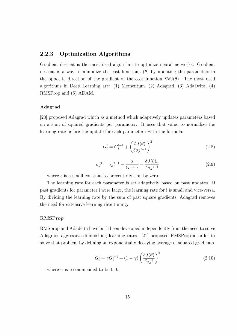
ADAM
[22] developed Adaptive Moment Estimation (ADAM) algorithm by combining Adamgrad
and RMSProp with a new implementation of Momemtum. It uses a decaying average
of squared gradients and a decaying average of past gradients:
mt = β1 ·mt−1 + (1− β1) · ∇J(θ) (2.11)
vt = β2 · vt−1 + (1− β2) · ∇J(θ)2 (2.12)
where mt and vt are estimates of the first moment (the mean) and the second
moment (the uncentered variance) of the gradients respectively. β1 and β2 are hyper-
parameters. Because mt and vt are initialized as zero vectors, this causes a biased
towards zero, especially during the initial time steps, and especially when the decay
rates are small due to β1 and β2 are close to 1. In order to solve this issue, the first
and second moment estimates are bias-corrected with:
mt =mt
1− βt1(2.13)
vt =vt
1− βt2(2.14)
and the final updating being:
θt = θt−1 − α ·mt
√vt + ε
(2.15)
2.3 Deep Reinforcement Learning
The curse of dimensionality given by large state and action spaces make unfeasible
to learn Q value estimates for each state and action pair independently as in normal
tabular Q-Learning. Therefore, Deep Reinforcement Learning (DRL) models the com-
ponents of RL with deep neural networks. The parameters of these networks are trained
by gradient descent to minimize some suitable loss function. The following subsections
describe the methods used for the current research to implement the proposed Deep
16

Reinforcement Learning in Traffic Light problem. More techniques are explained in
[23] and a benchmark of the aggregation of techniques is offered in [24].
2.3.1 Deep Q Networks
[25] proposed Deep Q-Networks (DQN) as a technique to combine Q-Learning with deep
neural networks where such technique proved to achieve super-human performance in
several Atari Games. This benchmark has become in the most common one.
Reinforcement learning is known to be unstable or even to diverge when a non-
linear function approximator such as a neural network is used to represent the Q value.
DQN addresses these instabilities by using two insights, experience replay and target
network.
The experience replay has three main advantages. Firstly, it allows greater data
efficiency because each step of experience is potentially used in many weight updates.
Secondly, learning directly from consecutive samples is inefficient, due to the correla-
tions between the samples; therefore, by randomizing the samples these correlations
can be broken and the variance of the updates can be reduced. Thirdly, when learning
on policy the current parameters determine the next data sample that the parameters
are trained on. By using this technique the behavior distribution is averaged over many
of the prior states, stabilizing the learning and avoiding fluctuations or divergence in
the parameters.
The another technique which improves the stability of neural networks is to use a
separate network to generating the targets yi during the Q-learning update. Specifi-
cally, every C updates the network Q is cloned in order to obtain a target network Q
and use Q for generating the Q-learning targets yi for the following C updates to Q. By
using this generations with older set of parameters it allows a delay between when an
update is done to Q and when that update affects the targets yi which makes unlikely
the presence of divergences or oscillations.
DQN parameterizes an approximate value function Q(s, a; θi) using CNN, where θi
are the weights of the network at iteration i. The experience replay stores the agent’s
experiences et = (st, at, rt, st+1) at each time step t in a dataset Dt = e1,,et pooled
over many episodes into a replay memory. Then, mini batches of experience drawn
uniformly at random from the dataset (s, a, r, s) ∼ U(D) are applied as Q-updates
17

during the training. The Q-learning update at iteration i follows the loss function:
Li(θi) = E(s,a,r,s)∼U(D)
[(r + γmax
a′Q(s′, a′; θ−i
)−Q (s, a; θi)
)2](2.16)
where θi are the parameters of the Q-network at iteration i and θ−i are the target
network parameters. The target network parameters are only updated with the Q-
network parameters every C steps and are held fixed between individual updates. The
Algorithm 1 states the procedure.
Algorithm 1: Deep Q-learning with Experience Replay
Initialize replay memory D to capacity NInitialize action-value function Q with random weights
Initialize target action-value function Q with weights θ− = θfor episode = 1, M do
Initialize sequence s1 = {x1} and preprocessed sequence φ1 = φ(s1)for t = 1, T do
With probability ε select a random action atotherwise select at = arg maxaQ(φ(st),a;θ)Execute action at in emulator and observe reward rt and image xt+1
Set st+ 1 = st,at,xt+1 and preprocess φt+1 = φ(st+1)Store transition (φt,at,rt,φt+1) in DSample random minibatch of transitions (φj,aj,rj,φj+1) from D
Set yj =
{rj, if episode terminates at step j + 1
r + γmaxa′ Q(φj+1, a′; θ−), otherwise
Perform a gradient descent step on (yj −Q(φj, aj; θ))2 with respect to the
network parameters θ
Every C steps reset Q = Q
2.3.2 Double DQN
The max operator in standard Q-learning and DQN uses the same values both to select
and to evaluate an action. It is known the this maximization sometimes produces to
learn unrealistically high action values which tends to prefer overestimated values over
18
underestimated values, resulting in overoptimistic value estimations. To prevent this,
Double Q-learning decouples the selection and the evaluation [26]. In this algorithm,
two value functions are learned by assigning each experience randomly to update one
of the two value functions, such that there are two sets of weights, θ and θ’. For each
update, one set of weights is used to determine the greedy policy and the other to
determine its value. After decoupling the selection and evaluation in Q-learning, the
Double Q-Learning error is formulated as:
Y DoubleQt = Rt+1 + γQ(st+1, arg max
aQ(st+1, a; θt); θ
′i) (2.17)
For DQN architectures is not desired to fully decoupled the target because the target
network provides a intuitive option for the second value function, without having to
include extra networks. For that reason, [27] propose to evaluate the greedy policy
according to the online network, but using the target network to estimate its value
given as result the Double DQN (DDQN) algorithm. Therefore, the DDQN can be
written as:
Y DDQNt = Rt+1 + γQ(st+1, arg max
aQ(st+1, a; θt); θ
−i ) (2.18)
The difference with the Double Q-learning is that the weights of the second network
θ′i are replaced with the weights of the target network θ−i for the evaluation of the
current greedy policy. The update to the target network works the same as normal
DQN.
2.3.3 Prioritized Experience Replay
[28] presented prioritized experience replay, a method that can make learning from
experience replay more efficient. Experience replay detaches online agents from pro-
cessing transitions in the exact order they are experienced. Prioritized replay detaches
agents from considering transitions with the same frequency that they are experienced.
[28] found that prioritized replay speeds up learning by a factor 2 in the performance
on the Atari benchmark. Prioritized replay samples more frequently transitions from
which there is a high expected learning progress. as measured by the magnitude of
their temporal-difference (TD) error. It samples transitions with probability pt relative
19

Algorithm 2: Dobuble DQN with proportional prioritization
Input: minibatch k, step size η, replay period K and size N, exponents α and β,budget T.
Initialize replay memory D = ∅, 4 = 0, piObserver S0 and choose A0 ∼ πθ(S0)for t = 1, T do
Observe St, R st, γtStore transition (St−1,At−1,Rt,γt,St) in D with maximum priority pt =maxi<t pi
if t ≡ 0 mod K thenfor j = 1, k do
Sample transition j /sim P(j) = pαj /∑
i pαi
Compute importance-sampling weight wj = (N · P(j))β / maxiwiCompute TD-error δj = Rj +γjQtarget(Sj, arg maxaQ(Sj, a))−Q(Sj−1, Aj−1)
Update transition priority pj ← |δj|Accumulate weight-change 4← 4 = wj · δj · ∇θQ(Sj−1, Aj−1)
Update weights θ ← θ + η · 4, reset4 = 0From time to time copy weights into target network θtarget ← θ
Choose action At ∼ πθ(St)
20

to the last encountered absolute TD error:
pt ∝∣∣∣(Rt+1 + γt+1 max
a′Q(s′, a′; θ−i
)−Q (s, a; θi)
)∣∣∣ω (2.19)
Where ω is a hyper-parameter that determines the pattern of the distribution. New
transitions are pushed into the replay buffer memory with maximum priority, providing
a bias towards recent transitions. Algorithm 2 describes the process for a proportional
prioritization.
2.3.4 Dueling Network
Dueling Network is a technique proposed by [2] which computes separately the value
V(s) and advantage A(s, a) functions that are represented by a duelling architecture
that consists of two streams where each stream represents one of these functions. These
two streams are combined by an convolutional layer to produce an estimate of the
state-action value Q(s, a) as shown in Figure 2.2. The dueling network automatically
produces separate estimates of the state value and advantage functions without super-
vision. Besides that, it can learn which states are valuable, without having to explore
the consequence of each action for each state.
The Q-values corresponds to the optimality of taking an action a given a state s
being Q(s, a). The Q-value can decomposed as:
Qπ(s, a) = V π(s) + A(s, a) (2.20)
where the state-value V π(s) describes how optimal is to be in a state s, and ad-
vantage A(s,a) expresses how more optimal is to take an action a compared to other
actions. The final equation used for dueling network is:
Q(s, a; θ, α, β) = V (s; θ, β) +
(A (s, a; θ, α)− 1
|A|∑a′
A (s, a; θ, α)
)(2.21)
21
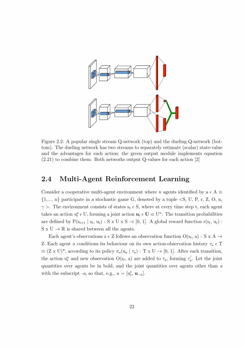
Figure 2.2: A popular single stream Q-network (top) and the dueling Q-network (bot-tom). The dueling network has two streams to separately estimate (scalar) state-valueand the advantages for each action; the green output module implements equation(2.21) to combine them. Both networks output Q-values for each action [2]
2.4 Multi-Agent Reinforcement Learning
Consider a cooperative multi-agent environment where n agents identified by a ε A ≡{1,..., n} participate in a stochastic game G, denoted by a tuple <S, U, P, r, Z, O, n,
γ >. The environment consists of states st ε S, where at every time step t, each agent
takes an action uat ε U, forming a joint action ut ε U ≡ Un. The transition probabilities
are defined by P(st+1 | st, ut) : S x U x S → [0, 1]. A global reward function r(st, ut) :
S x U → R is shared between all the agents.
Each agent’s observations z ε Z follows an observation function O(st, a) : S x A →Z. Each agent a conditions its behaviour on its own action-observation history τa ε T
≡ (Z x U)*, according to its policy πa(ua | τa) : T x U → [0, 1]. After each transition,
the action uat and new observation O(st, a) are added to τa, forming τ′a. Let the joint
quantities over agents be in bold, and the joint quantities over agents other than a
with the subscript -a, so that, e.g., u = [utt, u−a].
22
2.4.1 Independent DQN
Independent Q-Learning (IQL) was proposed in [29] to train agents independently while
each agent can learn its own policy by treating other agents as part of the environment.
Each agent learns its own Q-function that conditions only on the state and its own
action. IQL overcomes the scalability problems of centralised learning, but it introduces
the problem of the environment becoming nonstationary from the point of view of each
agent, as it involves other agents who are themselves learning at the same time, ruling
out any convergence guarantees [14].
Independent DQN (IDQN) is an extension of IQL with DQN for cooperative multi-
agent environment, where each agent a observes the partial state sat , selects an indi-
vidual action uat , and receives a team reward, rt shared among all agents. [30] com-
bines DQN with independent Q-learning, where each agent a independently and si-
multaneously learns its own Q-function Qa(s, ua; θai ) [31]. Since our setting is partially
observable, IDQN can be implemented by having each agent condition on its action-
observation history, i.e., Qa(τa, ua). In DRL, this can be implemented by given to each
agent a DQN on its own observations and actions.
As mentioned before, a key component of DQN is the experience replay memory.
Unfortunately, the combination of experience replay with IQL appears to be problem-
atic because the non-stationarity introduced by IQL which provokes that the dynamics
that generated the data in the agent’s experience replay memory no longer indicate
the current dynamics in which the agent is learning. IQL without a experience replay
memory can learn relatively well in spite of the non-stationarity so long as each agent
is able to progressively record the other agents’ policies, which it is not the case with a
experience replay memory enabled which is constantly confusing the agent with obso-
lete experiences. Besides that, disabling the experience replay memory as in [31], it is
not the optimal decision since it limits the sample efficiency and threats the stability
of multi-agent training. Experience replay not only stabilises the training, but it also
enhances the sample efficiency by constantly reusing experience tuples, therefore it is
important for DQN to use it.
23

2.4.2 Fingerprints
The technique was introduced by [14] along with another technique with importance
sampling similar to Prioritized Replay Experience. In the evaluations the fingerprint
method outperforms the importance sampling technique for feed forwards neural net-
works, which are the ones we use in this research.
[14] states that the disadvantage of IQL is that it ignores the changing over time
of the other agents’ policies because it perceives these other agents as part of the envi-
ronment, which cause non-stationarity on its own Q-function. Hence, the Q-function
might be made stationary if it conditioned on the other agents’ policies.
The idea to address this problem is to use something similar to hyper Q-learning
where each agent’s state space is resized with an estimate of the other agents’ policies
computed via Bayesian inference. The study discards the usage of the weights of the
other agents’ networks θ−a in the new observation, i.e. O’(st) = { O(st), θ−a }, because
is far too large to include as input to the Q-function due other agents -a are using DQN
as well. Although, a key insight is that each agent does not need to be able to condition
on any possible θ−a, but only on those values of θ−a that actually impact its experience
replay memory. The sequence of policies that generated the data in this buffer can be
interpreted as following an one-dimensional trajectory through the high-dimensional
policy space. In order to stabilise experience replay should be enough if each agent’s
observations disambiguate where this trajectory the training sample originated from.
Based on those points, a fingerprint must be correlated with the true value of state-
action pairs given the other agents’ policies. It should gradually change over training
time in order to allow the model to generalise across experiences in which the other
agents execute policies as they learn.
2.5 Deep Reinforcement Learning in Traffic Con-
trol
RL technique naturally models the dynamics of complex systems by learning the control
actions and the consequences of the traffic flow. It aims to get the optimal control
policy from the training in the exploration phase according to the inputs and outputs
observed. The harder part of reinforcement learning for traffic signal problems has been
24
in the exponentially increasing complexity of the dimensionality with respect to the
number of traffic signal states (the curse of dimensionality). The state space for traffic
control problems is so huge that becomes too expensive to solve the problem within a
finite time by using a table based Q learning method. Similarly, a traditional function
approximator based Q learning method has difficulties capturing the dynamics of traffic
flows. DL is being used to tackle this problem because it can simultaneously solve the
modeling and optimization problems of complex systems by using techniques such as
DQN. The combination of both RL and DL techniques enables to use multiple layers of
artificial neural networks to learn to choose the action that maximizes the discounted
future reward without prior knowledge of the environment for huge dimensionality
problems.
This section recaps previous works on traffic management, especially in traffic light
control, using Artificial Intelligence techniques. It comprises research applying novel
techniques for RL and DRL with both single and multiple agents. The first section
presents works in RL multi-agents dealing with the problem of need for coordination.
Then, it proceeds to more recent approaches that utilize DRL with single agents to
deal with the curse of dimensionality. Finally, the last section analyzes DRL with
multi-agents approaches not only for traffic lights but also for other UTC problems.
2.5.1 Multi-Agent Reinforcement Learning
Applying Multi-Agent Reinforcement Learning (MARL) for ATSC problem can be
challenging because the agents can adapt to changes in the environment at a local level
leading to non-collaborative learning and control, and therefore, a non-optimal global.
For that reason, besides the curse of dimensionality that ATSC suffers, MARL is also
challenged with the need of coordination among the multiple agents. The following
MARL approaches seek to achieve a collaborative result in order to learn a global
optimal policy between intersections. Table 2.1 summarizes the studies introduced in
this section.
[3] presents Realtime Adaptive Learning-based Traffic Control system (REALT),
which can simultaneously optimize multiple traffic management goals, learn suitable
junction collaboration parameters and optimize the learning and decision-making phases
by using a RL algorithm called Distributed W-Learning (DWL). DWL allows hetero-
25

Table 2.1: Existing research in Multi-Agent Reinforcement Learning for Traffic SignalControl
Research Algorithm State Action Phases Rewards
[3] DistributedW-Learning
Number of ve-hicles waitingand presenceof publictransportation
Ability to gen-erate multiplephase groups
Difference oftraffic countand no pres-ence of publictransportation
[32] Q-Learningand for learn-ing and min-sum commu-nication forsharing
Traffic condi-tions (i.e. rate,speed, and oc-cupancy)
2 Number on-road vehicles,average ofarriving ratesand average ofdeparting rate
[4] Swarm Re-inforcementLearning
Average queuelength
4 Number of ve-hicles waitingand crossing
[33] Q-Learning forlearning andMARLIN forcoordination
Queue length Mode de-pendent andconfigurable
Total Cumula-tive Delay
geneous intelligent agents to collaborate between each other in order to simultaneously
meet multiple heterogeneous policies. As can be seen from Figure 2.3, DWL manages
two levels of optimization: local agent optimization by using local policies and collab-
orative optimization by using remote policies. Each DWL agent uses Q-learning to
achieve its own local goals. Remote policies are learned by each agent using Q-learning
to realize how its local actions affect its nearest neighbors policies. Both local and re-
mote policies suggest an action to be executed at each time step. To mediate between
these two policies, an agent uses W-learning to learn importance of agents policies in
each state and it represents them as W values. The action with the highest W-value
for the current state is executed.
[32] introduces Min-sum Approximate Q-Learning (MAQL) which provides a multi-
agent distributed reinforcement learning where the agents achieves collaboration of a
global optimal goal by incorporating a distributed communication technique into RL
such that the learning and searching cost of large scale multi-agent systems can be
26

Figure 2.3: Distributed W-Learning [3]
significantly reduced. Specifically, it decomposes the global Q-learning function into
local Q-learning functions in order that each local agent can compute its own local
optimal policy based on local observations. Then, it applies the max-sum message
passing algorithm to share information between agents in order to find a stable and
optimal global policy that is used by all agents. The distributed RL is represented as a
factor graph where each variable node i ∈ V and each function node l := i ∈ Vi, and they
are connected by a function Ql. A max-sum algorithm is used for transferring messages
between local variable and function nodes, and achieving a cooperative joint control
among all the agents. In the paper, the algorithm is called the min-sum communication
because it minimizes the delayed cost function Ql. This algorithm performs directly on
the factor graph by specifying the messages that should be transferred across variable
and function nodes. In theory, the max-sum algorithm guarantees to converge to
the optimal global solution if the factor graph is acyclic. However, the factor graph
normally contains cycles in practice due to the mutual dependencies between agents.
Even though, there is evidence that shows max-sum algorithm can accomplish positive
results even in cyclic factor graphs.
[4] used a population based method called Particle Swarm Optimization which en-
ables to find efficiently the global optimal solution for multi-modal functions with wide
solution space. Particle swarm optimization is a population-based method originally
designed for continuous optimization problems. Agents learn through their local ex-
periences and by exchanging information among them. The agents interact in two
manners: (1) intra-level or horizontal interaction; where the agents interacts with each
27
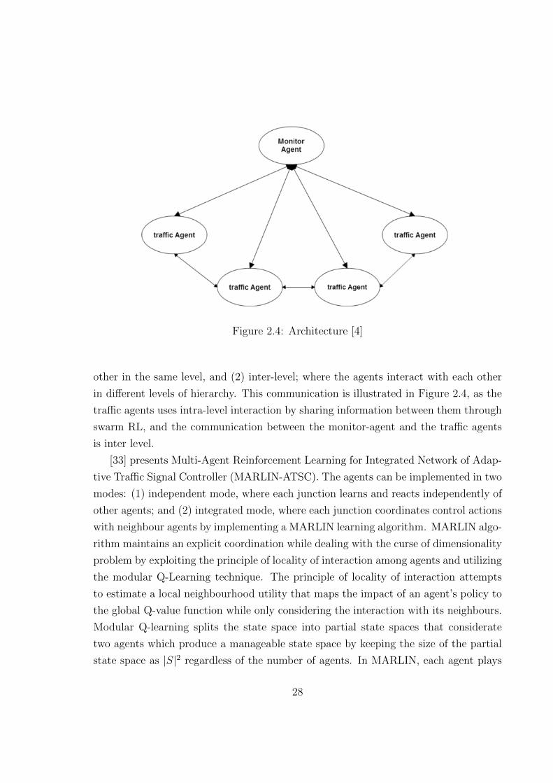
Figure 2.4: Architecture [4]
other in the same level, and (2) inter-level; where the agents interact with each other
in different levels of hierarchy. This communication is illustrated in Figure 2.4, as the
traffic agents uses intra-level interaction by sharing information between them through
swarm RL, and the communication between the monitor-agent and the traffic agents
is inter level.
[33] presents Multi-Agent Reinforcement Learning for Integrated Network of Adap-
tive Traffic Signal Controller (MARLIN-ATSC). The agents can be implemented in two
modes: (1) independent mode, where each junction learns and reacts independently of
other agents; and (2) integrated mode, where each junction coordinates control actions
with neighbour agents by implementing a MARLIN learning algorithm. MARLIN algo-
rithm maintains an explicit coordination while dealing with the curse of dimensionality
problem by exploiting the principle of locality of interaction among agents and utilizing
the modular Q-Learning technique. The principle of locality of interaction attempts
to estimate a local neighbourhood utility that maps the impact of an agent’s policy to
the global Q-value function while only considering the interaction with its neighbours.
Modular Q-learning splits the state space into partial state spaces that considerate
two agents which produce a manageable state space by keeping the size of the partial
state space as |S|2 regardless of the number of agents. In MARLIN, each agent plays
28

a Markov game [34, 35], also known as an Stochastic Game, with all its immediate
agents within its neighbourhood. Every agent has several learning modules where each
module corresponds to one game. Following the principle of modular Q-learning, the
state and action spaces are partitioned so that the agent can learn the joint policy with
one of the neighbours agents at a time.
Three out of the four approaches presented drew to a local learning first, to then
use a communication technique to either share or coordinate the learning across the
different agents. Only MARLIN-ATSC made usage of a different approach where the
agents learn along with its neighbors without any prior own local learning because this
study considered that the coordination can be achieved by taking into account the joint
state and joint action for the other agents. Besides that, only REALT allows to modify
the local goal independently, this is, the goals can be added, removed or modified, and
not all agents need to implement the same goals or have the same number of goals
which supports to handle different types of junctions.
Another interesting analysis to make is about the goals each work was trying to
optimize. Due to each goal in DWL is specified as an independent Q-learning process,
REALT implemented two policies: the first one is to optimize overall traffic flow by
rewarding positively if the overall traffic count at the current time-step is less than
at the previous time-step (i.e. the intersection cleared more traffic than it arrived in
the meantime), and the second is to prioritize special vehicles/buses, which rewards if
no special vehicle is waiting at any of its paths at decision time. On the other hand,
MAQL allows to each road of the simulated environment to be able to measure the real-
time traffic condition such as rate, speed, and occupancy. Besides that, each road has
a maximum capacity and a speed limit. Based on these conditions three parameters
can be estimated and targeted: (1) the number of on-road vehicles, (2) the moving
average of arriving rates and (3) the moving average of departing rates. In the case of
the Swarm RL, the reward function is based on the number of vehicles waiting in an
road of an intersection, and the number of vehicles crossed the junction coming from
another road of the intersection. It also used a penalty if the number of vehicles passing
over the roads is superior to the number of vehicles that are waiting for it. While in
MARLIN-ATSC, the reward is defined as the reduction in the total cumulative delay
associated with a junction, i.e., the difference between the total cumulative delays of
two successive decision points.
29

The final observation is about the evaluation and the results obtained in each study.
The Table 2 summarizes the environment for each work. First, REALT was rep-
resented in a simulation application called VISSIM which was set with 6 junctions,
using historical traffic and signal data of a real road network in Cork, Ireland. The
evaluation was against SCOOT, the traffic management system that controlled that
area. The performance comparison was done with three REALT settings and SCOOT
where the measured results were vehicle delay and number of stops. The three settings
of REALT outperformed SCOOT in low and medium traffic loads, however in high
loads the performance of SCOOT was better. In contrast, MAQL used the simulator
SUMO where simulated a traffic grid of 10x10 signalized intersections. It evaluated
the learning performance and convergence rate of MAQL using linear and sigmoid ap-
proximations. Then, it compared the performance of trained MAQL to decentralized
AQL (DAQL) method, which is the decentralized version of MAQL since each agent
learns independently without the message passing, and heuristic control methods .
The results demonstrated that the MAQL method had better performance than the
other approaches. It was also proved that DAQL method performed fast learning but
a greedy control. Additionally, DAQL and MAQL outperformed traditional heuristic
control models. Similar to MAQL, the Swarm RL research used SUMO but using four
junctions in a grid presentation with double lane edges. This research compared the
proposed method to a multi-agent architecture with standard Q-learning algorithm.
Results showed that the swarm Q-learning surpass the simple Q-learning causing less
average delay time and higher flow rate. Finally, MARLIN-ATSC used the simulator
PARAMICS with a network of 59 junctions of the lower downtown core of the City of
Toronto, ON, Canada, during the morning rush hour. The results demonstrated reduc-
tions in the average delay of 27% in independent mode and 39% in integrated mode.
Furthermore, the travel-time was decreased in 15% in independent mode and 26% in
integrated mode in the most congested roads in Downtown Toronto. An important
point to notice is that only two proposals, REALT and MARLIN-ATSC, were tested
with real traffic data.
30

Table 2.2: Test environments of existing research in Multi-Agent Reinforcement Learn-ing for Traffic Signal Control
Research Number of Junc-tions
Junction Struc-tures
Environment
[3] 6 Irregular. Allstructures aredifferent
VISSIM simulator.Real data of West-ern Road, Cork,Ireland.
[32] 100 Regular 10x10grid. All struc-tures are thesame
SUMO simulator
[4] 4 Regular. All struc-tures are the same
SUMO simulator
[33] 59 Irregular. Somejunctions have thesame structure butnot all
PARAMICS sim-ulator. Real dataof DowntownToronto, ON,Canada.
2.5.2 Single Agent Deep Reinforcement Learning
As mentioned before, DL helps to deal with the curse of dimensionality for complex
problems such as ASTC. This sections focuses only in single-agent approaches that
used DRL. The Table 2.3 shows a summary of the main aspects of previous works.
[5] made the estimation of Q-values with deep stacked autoencoders (SAE) neural
networks. The Figure 2.5 shows the architecture of this neural network which receives
as input the state and it outputs the Q-value for each possible action. The SAE neural
network contains several hidden layers of autoencoders where the outputs of each layer
is wired to the inputs of the successive layer. Autoencoder is a neural network that
defines the input and the target output to be the same. During Q-learning, the deep
SAE network is trained by minimizing the next loss function over samples of experience
until a specific time. The network was built with a four-layer SAE neural network and
two hidden layers. The hidden layers use a sigmoid activation function.
[36] proposed the combination of two RL algorithms: (1) deep policy-gradient (PG)
and (2) value-function based on a DNN, which perceives image observations in order
31
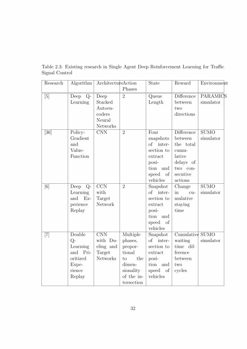
Table 2.3: Existing research in Single Agent Deep Reinforcement Learning for TrafficSignal Control
Research Algorithm ArchitectureActionPhases
State Reward Environment
[5] Deep Q-Learning
DeepStackedAutoen-codersNeuralNetworks
2 QueueLength
Differencebetweentwodirections
PARAMICSsimulator
[36] Policy-GradientandValue-Function
CNN 2 Foursnapshotsof inter-section toextractposi-tion andspeed ofvehicles
Differencebetweenthe totalcumu-lativedelays oftwo con-secutiveactions
SUMOsimulator
[6] Deep Q-Learningand Ex-perienceReplay
CCNwithTargetNetwork
2 Snapshotof inter-section toextractposi-tion andspeed ofvehicles
Changein cu-mulativestayingtime
SUMOsimulator
[7] DoubleQ-Learningand Pri-oritizedExpe-rienceReplay
CNNwith Du-eling andTargetNetworks
Multiplephases,propor-tionalto thedimen-sionalityof the in-tersection
Snapshotof inter-section toextractposi-tion andspeed ofvehicles
Cumulativewaitingtime dif-ferencebetweentwocycles
SUMOsimulator
32

Figure 2.5: The deep SAE neural network for approximating Q function [5]
to produce control signals in an isolated intersection. The PG based agent maps its
observation directly to the control signal; however, the value-function-based agent first
estimates values for all legal control signals. The agent then selects the optimal control
action with the highest value. The state of the system is an snapshot of the current
state of a graphical simulator, SUMO graphical user interface in this case. This image
is sent to a CNN such that the application can detect the location and the presence of
all vehicles in each lane. The history of consecutive observation is stacked in the CNN
as input to estimate the speed and direction of the vehicles. In PG, the policy is defined
as a mapping from the input state to a probability distribution over the action space
where this policy distribution is learned with DNN by performing gradient descent on
the policy parameters. Meanwhile, in the value function-based algorithm, the DNN is
used to estimate the action-value function. The action-value-function maps the input
state to action values that represent the future reward that can be obtained by doing the
given action from the given state. The network was employed with two convolutional
layers and one fully connected layer. All three layers are activated with some non-linear
function that is not specified.
33

Figure 2.6: DNN structure. Note that the small matrices and vectors in this figureare for illustration simplicity, whose dimensions should be set accordingly in DNNimplementation [6]
[6] proposed the usage of a DQN with experience replay and target network meth-
ods to improve the stability. The Figure 3.4 shows the architecture of the DNN as
follows: the state consists of the position and speed of vehicles that are fed to the CNN
as matrices P and V respectively. Each one of these matrices pass through two convo-
lutional layers that are activated with the ReLU function. Then, a traffic signal state
vector L is aggregated to the outputs of the two aforementioned networks, forming the
input of the third layer. The third and fourth layers are fully connected layers that are
also activated with ReLU functions. The output layer is another fully connected layer
that returns a vector of Q-values.
Figure 2.7 shows how an agent is trained in this model. The agent records observed
interaction experience into a replay memory M. Additionally, it used the estimated
Q-value from the DNN as the input of a target network to best approximate the
optimal Q-value. This target network has the same architecture as the DNN. It used
34
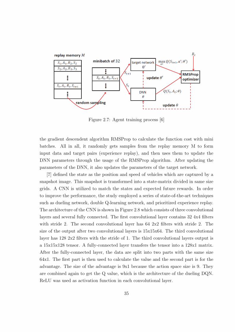
Figure 2.7: Agent training process [6]
the gradient descendent algorithm RMSProp to calculate the function cost with mini
batches. All in all, it randomly gets samples from the replay memory M to form
input data and target pairs (experience replay), and then uses them to update the
DNN parameters through the usage of the RMSProp algorithm. After updating the
parameters of the DNN, it also updates the parameters of the target network.
[7] defined the state as the position and speed of vehicles which are captured by a
snapshot image. This snapshot is transformed into a state-matrix divided in same size
grids. A CNN is utilized to match the states and expected future rewards. In order
to improve the performance, the study employed a series of state-of-the-art techniques
such as dueling network, double Q-learning network, and prioritized experience replay.
The architecture of the CNN is shown in Figure 2.8 which consists of three convolutional
layers and several fully connected. The first convolutional layer contains 32 4x4 filters
with stride 2. The second convolutional layer has 64 2x2 filters with stride 2. The
size of the output after two convolutional layers is 15x15x64. The third convolutional
layer has 128 2x2 filters with the stride of 1. The third convolutional layers output is
a 15x15x128 tensor. A fully-connected layer transfers the tensor into a 128x1 matrix.
After the fully-connected layer, the data are split into two parts with the same size
64x1. The first part is then used to calculate the value and the second part is for the
advantage. The size of the advantage is 9x1 because the action space size is 9. They
are combined again to get the Q value, which is the architecture of the dueling DQN.
ReLU was used as activation function in each convolutional layer.
35
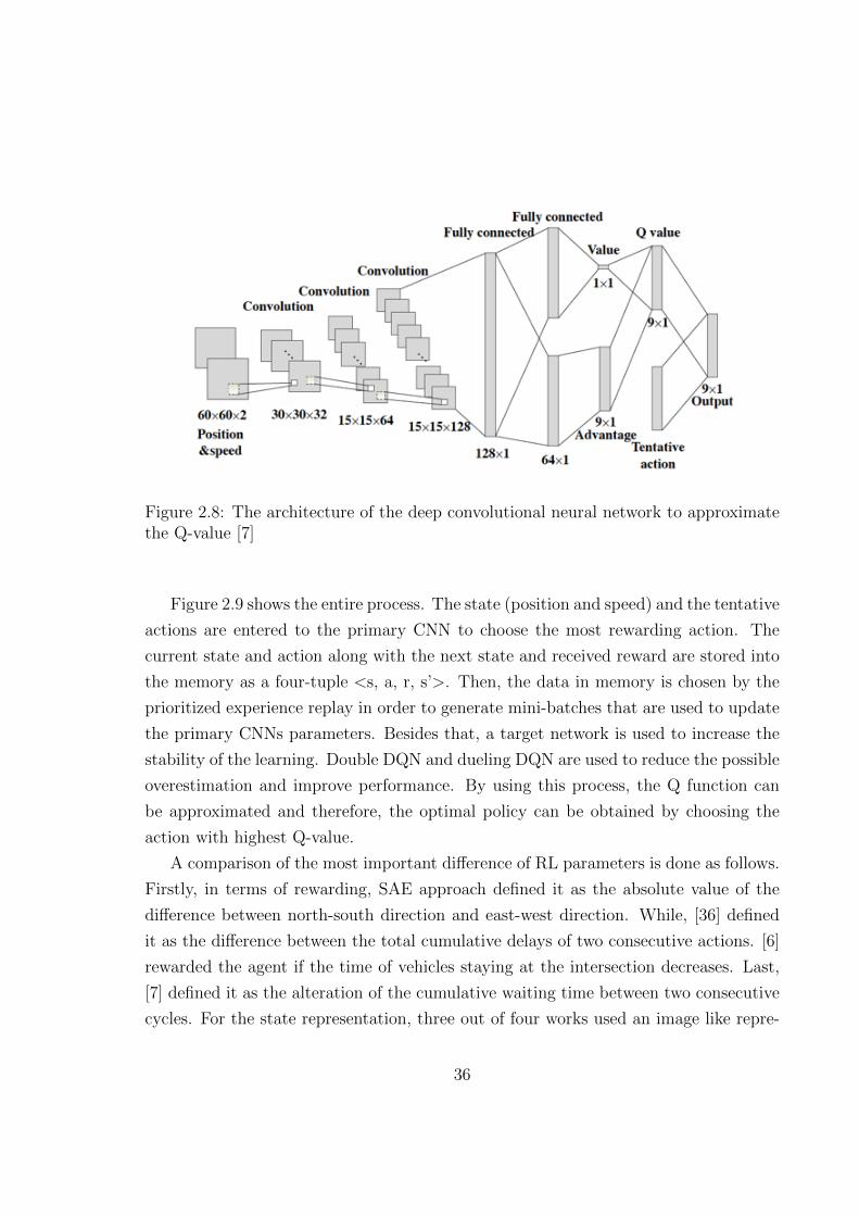
Figure 2.8: The architecture of the deep convolutional neural network to approximatethe Q-value [7]
Figure 2.9 shows the entire process. The state (position and speed) and the tentative
actions are entered to the primary CNN to choose the most rewarding action. The
current state and action along with the next state and received reward are stored into
the memory as a four-tuple <s, a, r, s’>. Then, the data in memory is chosen by the
prioritized experience replay in order to generate mini-batches that are used to update
the primary CNNs parameters. Besides that, a target network is used to increase the
stability of the learning. Double DQN and dueling DQN are used to reduce the possible
overestimation and improve performance. By using this process, the Q function can
be approximated and therefore, the optimal policy can be obtained by choosing the
action with highest Q-value.
A comparison of the most important difference of RL parameters is done as follows.
Firstly, in terms of rewarding, SAE approach defined it as the absolute value of the
difference between north-south direction and east-west direction. While, [36] defined
it as the difference between the total cumulative delays of two consecutive actions. [6]
rewarded the agent if the time of vehicles staying at the intersection decreases. Last,
[7] defined it as the alteration of the cumulative waiting time between two consecutive
cycles. For the state representation, three out of four works used an image like repre-
36
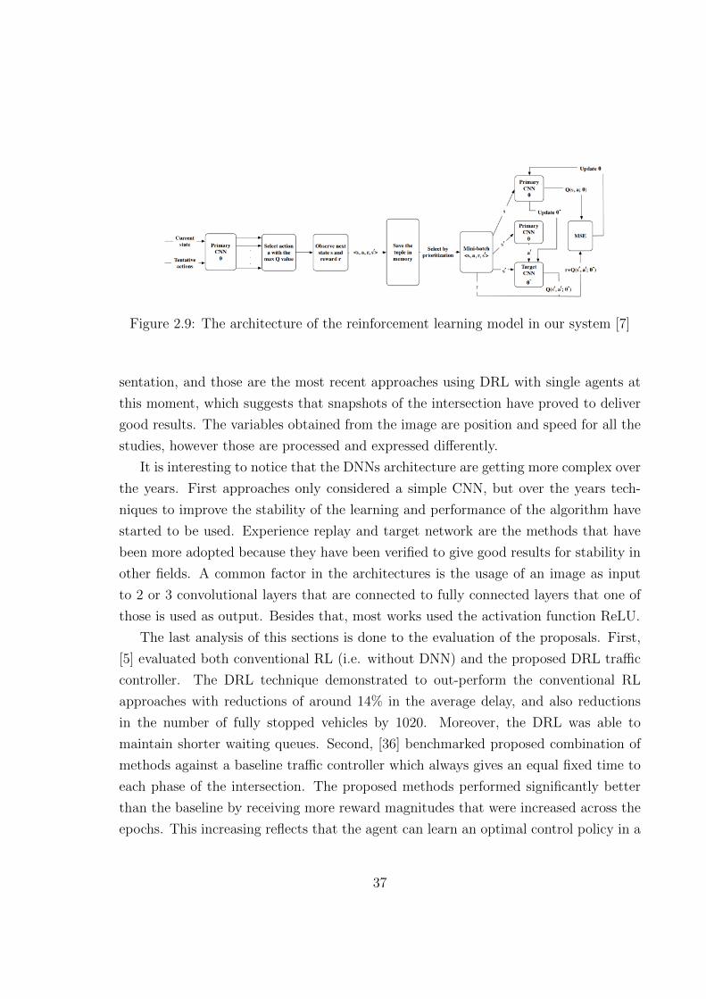
Figure 2.9: The architecture of the reinforcement learning model in our system [7]
sentation, and those are the most recent approaches using DRL with single agents at
this moment, which suggests that snapshots of the intersection have proved to deliver
good results. The variables obtained from the image are position and speed for all the
studies, however those are processed and expressed differently.
It is interesting to notice that the DNNs architecture are getting more complex over
the years. First approaches only considered a simple CNN, but over the years tech-
niques to improve the stability of the learning and performance of the algorithm have
started to be used. Experience replay and target network are the methods that have
been more adopted because they have been verified to give good results for stability in
other fields. A common factor in the architectures is the usage of an image as input
to 2 or 3 convolutional layers that are connected to fully connected layers that one of
those is used as output. Besides that, most works used the activation function ReLU.
The last analysis of this sections is done to the evaluation of the proposals. First,
[5] evaluated both conventional RL (i.e. without DNN) and the proposed DRL traffic
controller. The DRL technique demonstrated to out-perform the conventional RL
approaches with reductions of around 14% in the average delay, and also reductions
in the number of fully stopped vehicles by 1020. Moreover, the DRL was able to
maintain shorter waiting queues. Second, [36] benchmarked proposed combination of
methods against a baseline traffic controller which always gives an equal fixed time to
each phase of the intersection. The proposed methods performed significantly better
than the baseline by receiving more reward magnitudes that were increased across the
epochs. This increasing reflects that the agent can learn an optimal control policy in a
37

stable way. Another evaluation was done using a Shallow Neural Network (SNN) which
only has one hidden layer. It demonstrated that the proposed models outperformed
the SNN method by reducing in 67% the average cumulative delay and 72% the queue
length for the PG method; while reductions of 68% in the average cumulative delay
and 73% in the queue length for the value-function-based method. Third, [6] examined
the learning performance, which converge and keeps stable after 800 episodes. Then, it
compared the vehicle delay performance of the proposed algorithm to that of another
two algorithms: (1) longest queue first algorithm and (2) fixed time control algorithm.
It demonstrated a reduction up to 86% compared to fixed time control algorithm and
up to 47% longest queue first algorithm for two out of four roads tested. The other
two roads the proposed research did not get good results. Finally, [7] compared the
proposed model against a pre-scheduled traffic signal. The propose demonstrated the
capability to learn a good policy under both the rush hours and normal traffic flow
rates. Moreover, it showed to reduce around 20% of the average waiting timing from
the starting training compared to the other strategy. It is important to notice that any
of these works were evaluated with real data.
2.5.3 Multi-Agent Deep Reinforcement Learning
This section covers the usage of DRL in multi-agents scenarios. The following studies
attempt to deal with the main challenges of ASTC. The proposed work will try to
outperforms the following studies. Table 2.4 summarizes the characteristics of the
existing approaches.
[8] used DRL for controlling the metering of highway on-ramps modelling the prob-
lem as discretized non-linear partial differential equations (PDEs) in a robust and
non-parametric manner. DRL enables the management of discretized PDEs whose pa-
rameters are unknown, random, and time-varying. The DNN architecture consists of a
nx3 array, where n is the number of discretization cells of the roadway in the simulator,
and every of these cells contain three variables: (1) the vehicle density scaled to a me-
dian value of 0, and a standard deviation of 1 in average, (2) a boolean value indicating
whether an off-ramp is present or not, and (3) a logarithmic scaled value that indicates
the number of vehicles standing by in the on-ramp queue if there is any, 0 otherwise.
Each agent examines a near discretized region of the highway with these three values
38
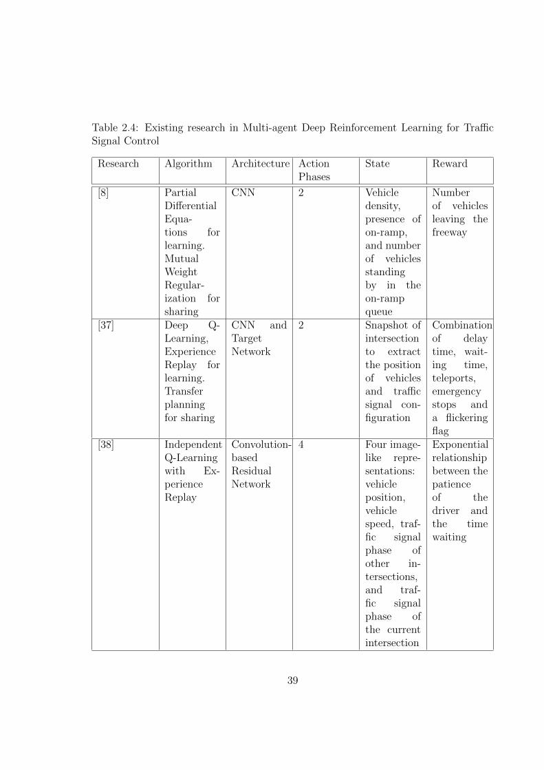
Table 2.4: Existing research in Multi-agent Deep Reinforcement Learning for TrafficSignal Control
Research Algorithm Architecture ActionPhases
State Reward
[8] PartialDifferentialEqua-tions forlearning.MutualWeightRegular-ization forsharing
CNN 2 Vehicledensity,presence ofon-ramp,and numberof vehiclesstandingby in theon-rampqueue
Numberof vehiclesleaving thefreeway
[37] Deep Q-Learning,ExperienceReplay forlearning.Transferplanningfor sharing
CNN andTargetNetwork
2 Snapshot ofintersectionto extractthe positionof vehiclesand trafficsignal con-figuration
Combinationof delaytime, wait-ing time,teleports,emergencystops anda flickeringflag
[38] IndependentQ-Learningwith Ex-perienceReplay
Convolution-basedResidualNetwork
4 Four image-like repre-sentations:vehicleposition,vehiclespeed, traf-fic signalphase ofother in-tersections,and traf-fic signalphase ofthe currentintersection
Exponentialrelationshipbetween thepatienceof thedriver andthe timewaiting
39
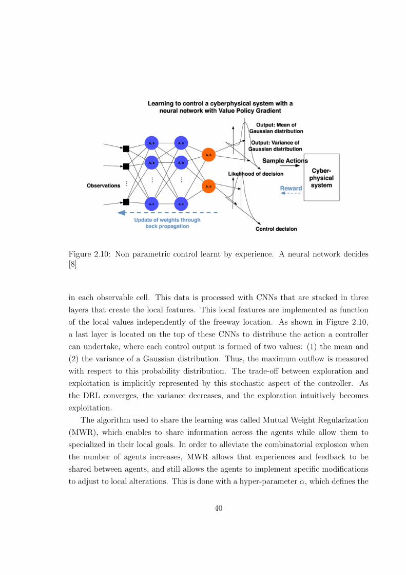
Figure 2.10: Non parametric control learnt by experience. A neural network decides[8]
in each observable cell. This data is processed with CNNs that are stacked in three
layers that create the local features. This local features are implemented as function
of the local values independently of the freeway location. As shown in Figure 2.10,
a last layer is located on the top of these CNNs to distribute the action a controller
can undertake, where each control output is formed of two values: (1) the mean and
(2) the variance of a Gaussian distribution. Thus, the maximum outflow is measured
with respect to this probability distribution. The trade-off between exploration and
exploitation is implicitly represented by this stochastic aspect of the controller. As
the DRL converges, the variance decreases, and the exploration intuitively becomes
exploitation.
The algorithm used to share the learning was called Mutual Weight Regularization
(MWR), which enables to share information across the agents while allow them to
specialized in their local goals. In order to alleviate the combinatorial explosion when
the number of agents increases, MWR allows that experiences and feedback to be
shared between agents, and still allows the agents to implement specific modifications
to adjust to local alterations. This is done with a hyper-parameter α, which defines the
40

weight of the regularization, and consequently how much mutual information is shared
between agents. Where α = 0 is equals to having independent policies for every agent,
and α = ∞ is equivalent to having a shared policy making algorithm for every agent.
[37] designed a DQN solution which uses experience replay and target network to
stabilize the learning. It represents the state as image that then is transform into a
binary matrix of the position of the vehicles with additional information of the traffic
lights configuration. The paper does not provides details about the DNN architecture.
The solution to multi-agents is made with transfer planning and max-plus algorithms.
Transfer planning allows to learn the Q-function for a sub-problem of a multi-agent
problem that later can be reused for the other similar subproblems by exploiting the
symmetries. Therefore, this algorithm only works for intersections that are equal. The
max-plus algorithm is used for coordination of the multi-agents in order to optimize
the joint global action over the entire coordination graph.
[38] presented Cooperative Deep Reinforcement Learning (CDRL), a multi-agent
framework that used a convolution-based residual network (ResNet) to speed up the
training process while providing reasonable results. It made use of Independent Q-
Learning (IQL) and Experience Replay. In IQL, each agent learns its own policy
independently and it considers other agents as part of the environment. Also, the
agents are able to track the policies of other agents in real time. To deal with non-
stationarity, only one junction will be trained at each training episode, the others will
react based on their previously learned policies. During training phase, the agent does
not communication with the other agents. Four image-like matrices are the state and
input of the DNN for each agent. However, only one agent will receive the reward
during each training cycle, and only the ResNet and replay memory of that agent is
updated. After an amount of iterations, the latest agent’s policy is distributed to the
other agents, and the training agent is changed to another one to start a new training
cycle.
The studies did not present plenty information about the DNN architecture. One
thing that can be noticed from two out of three works is that the tendency of using
image-like representation for the state is still used in multi-agent environments be-
cause it captures better the traffic light problem parameters. Furthermore, the same
two works used Experience Replay as single agents proposals in order to stabilize the
learning, however the usage of this technique is more complex in multi-agents. Both
41

studies isolated the training either to one agent level or to the minimal sub-problem
(coordination of two agents). As a consequence of this segregation, the topology of the
junctions is the same where they used a four intersection in a nine cell grid (#) sce-
nario producing the same intersection structure for all the agents, and the main reason
IQL and transfer planning worked. The presented work will attempt to overcome that
difficulty and to use an irregular topology.
Table 2.5: Test environments of existing research in Multi-agent Deep ReinforcementLearning for Traffic Signal Control
Research Number of Junc-tions
Junction Struc-tures
Environment
[8] *29 on-ramps, notjunctions
Irregular. Someon-ramps have thesame structure butnot all
BeATS simulator.210 Eastboundfreeway in south-ern California.
[37] 4 Regular. All struc-tures are the same
SUMO simulator
[38] 4 Regular. All struc-tures are the same
SUMO simulator
A comparison of the evaluation and results is presented as follows. [8] used real
data of 33 km of the 210 Eastbound freeway in southern California. The proposed
approach was benchmarked against 3 systems: (1) a baseline without any ramp meter-
ing, (2) the proposed DRL approach without MWR technique and (3) ALINEA, the
current state-of-the-art system used in the place. Two evaluation were made where
the MWR approach provides an important improvement compared to the baseline ant
he NOMWR approaches, however it did not outperform ALINEA. [37] compared the
proposal against a combination of two previous works that called Wiering/Kuyer. The
evaluation of this study did not present outstanding results neither. The proposed
approach outperforms the Wiering/Kuyer approach most of the time, but due to insta-
bility, it sometimes underperforms, especially in the four-agent case. Also, they found
a problem with the activation of the convolutional filters, these filters did not detect
vehicles after a while, even when vehicles are present. As a consequence, a traffic jam
is produced because the agent no longer switches lights. [38] evaluated CDRL against
three baselines algorithms: (1) Self-Organizing Traffic Lights (SOTL), a controller that
42

switches the lights according to the elapsed time and the queue length, (2) Q-Learning,
regular RL method, (3) DQN, each agent determines the alternation of action phase
only taking into account local traffic situations. The experiments demonstrated that
CDRL is the technique that converges slowest but once the convergence is complete,
CDRL behaves better than other techniques. Besides that, the performance of CDRL
in some experiments confirmed the importance of cooperation in multi-agent environ-
ments.
2.6 Summary
This chapter presented the key techniques used for the current research. It introduced
the concept of RL and its extension to DL as DRL. Then, it explained the different
state-of-the-art methods for Deep Q-Learning by using DQN and its aggregated tech-
niques which enhance the stability and performance of the training. Besides that, it
described the extension of DRL to our multi-agent setting and the technique we pro-
pose to overcome the non-stationarity in heterogeneous multi-agent UTC systems. The
chapter 3 and 4 explains in more detail the design and implementation, respectively,
of these key components.
In this chapter we presented related works in UTC for single and multiple agents.
The first subsection described some of the RL techniques used for multi-agents. Then
we presented the evolution of approach towards the usage of DL techniques to address
the curse of dimensionality. Firstly, we showed some works for single agent and then a
few multi-agent studies. From the latest works in multi-agent for UTC using DRL, we
noticed that none of the DQN approaches try to address a heterogeneous environment,
and they presented problems with the non-stationarity of the environment. We focus
our research on overcome these two issues as our contribution of the work as mentioned
in Chapter 1.
43

Chapter 3
Design
This chapter outlines the approach used to design the different components of the
Traffic Light Control problem as a RL problem. This section explains the applied algo-
rithms to tackle the problem of single and multiple intersections. It includes the design
of the Neural Network architecture as well as the algorithms and techniques applied
to train single and multiple agents in order to achieve a collaborative environment. It
presents the design of the proposed IDQN for the UTC in a heterogeneous multi-agent
environment in order to overcome the non-stationarity. Besides that, it presents and
justifies the design decisions taken when selecting different DQN techniques and RL
components. It presents the results of preliminary experiments performed in order to
determine the most suitable DRL techniques and RL components.
3.1 Traffic Light Control Problem
The Traffic Light Control problem is formulated as a RL problem where an agent
interacts with the environment which is a partial section of the road network which
contains the intersection with the traffic light that it is intended to manage at discrete
time steps t. Specifically, the agent observes an state st ∈ S at the beginning of a
time step t, then it chooses and actuates an action at ∈ A which corresponds to one
of the configurations the traffic signal can take. After taking the action at, the agent
transitions to the next state st+1 ∈ S and receives a reward rt. The next subsections
define these components.
44
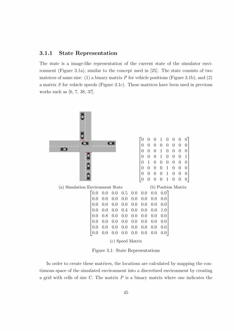
3.1.1 State Representation
The state is a image-like representation of the current state of the simulator envi-
ronment (Figure 3.1a), similar to the concept used in [25]. The state consists of two
matrices of same size: (1) a binary matrix P for vehicle positions (Figure 3.1b), and (2)
a matrix S for vehicle speeds (Figure 3.1c). These matrices have been used in previous
works such as [6, 7, 38, 37].
(a) Simulation Environment State
0 0 0 1 0 0 0 00 0 0 0 0 0 0 00 0 0 1 0 0 0 00 0 0 1 0 0 0 10 1 0 0 0 0 0 00 0 0 0 1 0 0 00 0 0 0 1 0 0 00 0 0 0 1 0 0 0
(b) Position Matrix
0.0 0.0 0.0 0.5 0.0 0.0 0.0 0.00.0 0.0 0.0 0.0 0.0 0.0 0.0 0.00.0 0.0 0.0 0.0 0.0 0.0 0.0 0.00.0 0.0 0.0 0.4 0.0 0.0 0.0 1.00.0 0.8 0.0 0.0 0.0 0.0 0.0 0.00.0 0.0 0.0 0.0 0.0 0.0 0.0 0.00.0 0.0 0.0 0.0 0.0 0.0 0.0 0.00.0 0.0 0.0 0.0 0.0 0.0 0.0 0.0
(c) Speed Matrix
Figure 3.1: State Representations
In order to create these matrices, the locations are calculated by mapping the con-
tinuous space of the simulated environment into a discretized environment by creating
a grid with cells of size C. The matrix P is a binary matrix where one indicates the
45
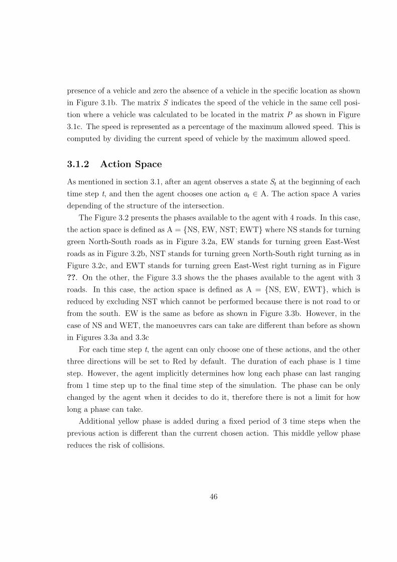
presence of a vehicle and zero the absence of a vehicle in the specific location as shown
in Figure 3.1b. The matrix S indicates the speed of the vehicle in the same cell posi-
tion where a vehicle was calculated to be located in the matrix P as shown in Figure
3.1c. The speed is represented as a percentage of the maximum allowed speed. This is
computed by dividing the current speed of vehicle by the maximum allowed speed.
3.1.2 Action Space
As mentioned in section 3.1, after an agent observes a state St at the beginning of each
time step t, and then the agent chooses one action at ∈ A. The action space A varies
depending of the structure of the intersection.
The Figure 3.2 presents the phases available to the agent with 4 roads. In this case,
the action space is defined as A = {NS, EW, NST; EWT} where NS stands for turning
green North-South roads as in Figure 3.2a, EW stands for turning green East-West
roads as in Figure 3.2b, NST stands for turning green North-South right turning as in
Figure 3.2c, and EWT stands for turning green East-West right turning as in Figure
??. On the other, the Figure 3.3 shows the the phases available to the agent with 3
roads. In this case, the action space is defined as A = {NS, EW, EWT}, which is
reduced by excluding NST which cannot be performed because there is not road to or
from the south. EW is the same as before as shown in Figure 3.3b. However, in the
case of NS and WET, the manoeuvres cars can take are different than before as shown
in Figures 3.3a and 3.3c
For each time step t, the agent can only choose one of these actions, and the other
three directions will be set to Red by default. The duration of each phase is 1 time
step. However, the agent implicitly determines how long each phase can last ranging
from 1 time step up to the final time step of the simulation. The phase can be only
changed by the agent when it decides to do it, therefore there is not a limit for how
long a phase can take.
Additional yellow phase is added during a fixed period of 3 time steps when the
previous action is different than the current chosen action. This middle yellow phase
reduces the risk of collisions.
46

(a) North-South (b) East-West
(c) North-South Turn (d) East-West Turn
Figure 3.2: Traffic light phases available to agent with 4 roads
47
(a) North-South (b) East-West
(c) East-West Turn
Figure 3.3: Traffic light phases available to agent with 3 roads
48

3.1.3 Reward Function
The definition of the reward function is one of the hardest part of RL. Therefore,
we evaluate several functions in order to choose a reward function that converges to
optimal policy. A reward is a scalar value rt ∈ R that is returned after the agent takes
an action at in the environment at each time step t.
Let wi,t be the ith vehicle’s waiting time at time step t, and Wt the total cumulative
waiting time for all the vehicles in the observation scope of the road network at time
step t as shows in equation 3.1. The reward function is formulated in equation 3.2.
The intention of the reward function is to reward positive the agent in a range (0.0,
1.0] where the agent’s reward loses value proportional to the cumulative waiting time
at time step t. Thus, the agent must keep short waiting time in order to receive higher
scores, and as consequence, this reward function accomplishes the goal of reducing the
driver’s waiting time at a junction.
Wt =∑i
wi,t (3.1)
rt =
1.0Wt, if cummulative waiting time Wt is greater than 0
1.0, otherwise(3.2)
The second option of rewarding is to use the difference of cumulative waiting time of
two consecutive time steps, namely t-1 and t, as it has been applied in [36, 6, 7]. This
reward function uses the same definition ofWt as shows in 3.1. Let beWt the cumulative
waiting time for the current time step being t and Wt−1 the cumulative waiting time
for the previous time step being t-1. This rewards seeks to reward positively the agent
when it reduces the waiting time for two consecutive time steps because this can be
translated to a relief in the traffic congestion in the intersection. On the other hand,
when the waiting time from two consecutive increases, the difference will be a negative
reward and thus it will penalize the agent because it is incrementing the waiting time.
Hence, the reward function is formulated as in equation 3.3.
rt = Wt−1 −Wt (3.3)
We tested both reward functions in order to chose the reward that get us the best
49

policy. The table 3.1 shows the hyperparameters used for the executions. The Figure
3.4 shows the comparison of both reward functions. As can been seen from figures 3.4b
and 3.4a, the first aforementioned function works undoubtedly better than the second
one by reducing significantly more both, the average waiting time and the average
waiting time. Based on these results, we decide to use the reward function of equation
3.2.
Table 3.1: DRL techniques evaluation hyper-parameters
Parameter Value
Episodes 1000Time steps 3600000Pre train time steps 2000learning rate 0.0004Exploration ε 1.0 → 0.01Time steps from starting ε to ending ε 360000Target network update 3000Prioritization exponent α 0.6Prioritization importance sampling β 0.4 → 1.0Discount factor γ 0.99Replay Memory size M 50000Minibatch size B 32
(a) Average Waiting Time per Episode (b) Average Travel Time per Episode
Figure 3.4: Reward Functions Experiment
50
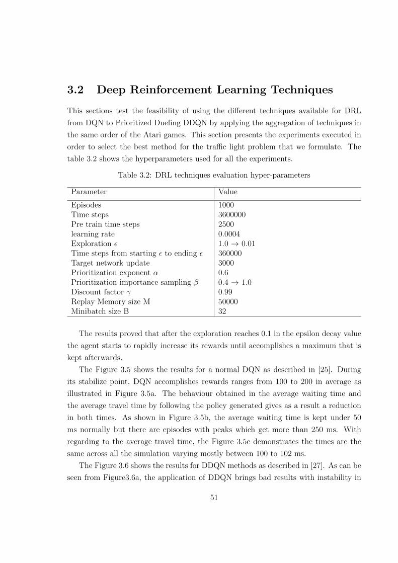
3.2 Deep Reinforcement Learning Techniques
This sections test the feasibility of using the different techniques available for DRL
from DQN to Prioritized Dueling DDQN by applying the aggregation of techniques in
the same order of the Atari games. This section presents the experiments executed in
order to select the best method for the traffic light problem that we formulate. The
table 3.2 shows the hyperparameters used for all the experiments.
Table 3.2: DRL techniques evaluation hyper-parameters
Parameter Value
Episodes 1000Time steps 3600000Pre train time steps 2500learning rate 0.0004Exploration ε 1.0 → 0.01Time steps from starting ε to ending ε 360000Target network update 3000Prioritization exponent α 0.6Prioritization importance sampling β 0.4 → 1.0Discount factor γ 0.99Replay Memory size M 50000Minibatch size B 32
The results proved that after the exploration reaches 0.1 in the epsilon decay value
the agent starts to rapidly increase its rewards until accomplishes a maximum that is
kept afterwards.
The Figure 3.5 shows the results for a normal DQN as described in [25]. During
its stabilize point, DQN accomplishes rewards ranges from 100 to 200 in average as
illustrated in Figure 3.5a. The behaviour obtained in the average waiting time and
the average travel time by following the policy generated gives as a result a reduction
in both times. As shown in Figure 3.5b, the average waiting time is kept under 50
ms normally but there are episodes with peaks which get more than 250 ms. With
regarding to the average travel time, the Figure 3.5c demonstrates the times are the
same across all the simulation varying mostly between 100 to 102 ms.
The Figure 3.6 shows the results for DDQN methods as described in [27]. As can be
seen from Figure3.6a, the application of DDQN brings bad results with instability in
51
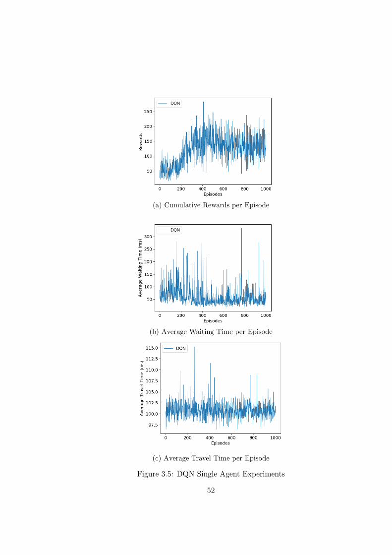
(a) Cumulative Rewards per Episode
(b) Average Waiting Time per Episode
(c) Average Travel Time per Episode
Figure 3.5: DQN Single Agent Experiments
52

(a) Cumulative Rewards per Episode
(b) Average Waiting Time per Episode
(c) Average Travel Time per Episode
Figure 3.6: DDQN Single Agent Experiments
53

the rewards which goes down until 50, which is 100% less that the minimum recorded
with DQN in its stability point. This issue was also seen in [37] where the study
suggests that, regardless of the state, DDQN assigns highly identical Q-values to all
actions. Despite of the instability of rewarding, the average waiting time and travel
time do not seems to be affected directly for this, they have a constant performance
even though it is poor performance in comparison with DQN. Figure 3.6b DDQN gets
twice the waiting time of DQN attaining values before 100 ms but higher than 50 ms.
The results of waiting travel time in Figure 3.6c are similar to DQN reaching between
100 and 105 ms approximately.
The Figure 3.7 shows the results of the Prioritized DDDQN as described in [28].
The Figure 3.7a illustrates that this technique gets to converge faster by reaching its
maximum around 300 episodes unlike the DQN and DDQN which reaches convergence
around 400 episodes. This shows the Prioritization Experience Replay helps the DDQN
with the instability issues, however the combination of this two techniques gets a very
similar performance than DQN in terms of rewarding. As can be seen from Figure 3.7b,
Prioritized DDQN makes better work keeping the waiting time under 50 ms without so
many increments in other episodes unlike DQN, thus it slightly outperforms DQN. In
terms of the travel time, the Figure 3.7c shows a similar performance than DQN with
an improvement in the stability of the learning. This is result of sampling experience
with high expected learning progress, which speeds up the learning, and thus the agent
can converge and generalize faster.
The Figure 3.8 shows the results of using Prioritized Dueling DDQN as described
in [2]. The Figure 3.8a shows how this technique converges slower at around 500
episodes where it reaches the highest rewards, however after that, it behaves more
stable achieving more constant similar values from consequent episodes and scoring
high rewards in the range of 120-200. The Figure 3.8b shows that this technique has a
similar effect as Prioritized DDQN for the average waiting time, it tends to accomplishes
waiting times below of 50 ms with few spikes of up to 100 ms, this demonstrates the
stability of the policy. The Figure 3.8c presents similar range of average travel time
which goes from 98 to 103 ms, nevertheless it behaves more stable (no presence of
spikes) after convergence.
After this experiments we concluded that the usage of Prioritized Dueling DDQN
provides a more stable behaviour, however the performance does not increase signifi-
54
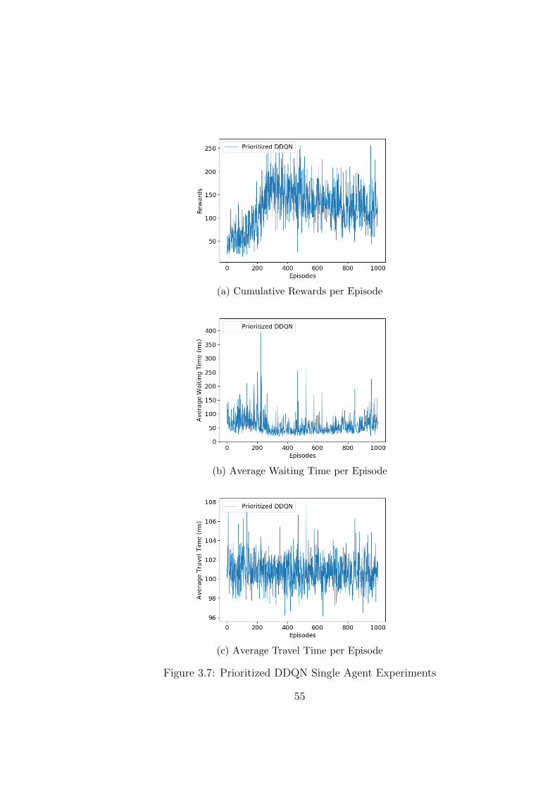
(a) Cumulative Rewards per Episode
(b) Average Waiting Time per Episode
(c) Average Travel Time per Episode
Figure 3.7: Prioritized DDQN Single Agent Experiments
55

(a) Cumulative Rewards per Episode
(b) Average Waiting Time per Episode
(c) Average Travel Time per Episode
Figure 3.8: Prioritized Dueling DDQN Single Agent Experiments
56

cantly compare to the previous techniques. Despite the fact that the performance do
not suffer a important increase, we decide to use Prioritized Dueling DDQN because of
the stability it offers which can be very useful in the multi-agent scenario where stability
issues can be harder to handle because the increasing of agents and its non-stationary.
3.3 Deep Neural Network Architecture
Figure 3.9: The architecture of the Deep Neural Network.
The neural network used to train the agent for single and multi-agent environments
is the same as [2]. This neural network was used for all the experiments performed
during this research, except for the experimentation of techniques elaborated in 3.2.
Only the Prioritized Dueling DDQN uses this architecture, the other techniques use
a similar architecture without the split of the last layer which is the application of
Dueling Network as explained in section 2.3.4.
The Figure 3.9 illustrates the Deep Neural Network. There are 3 convolutional
layers followed by 2 fully-connected layers. The first convolutional layer has 32 8x8
filters with stride 4. The second convolutional layer has 64 4x4 filters with stride 2.
The third and final convolutional layer has 64 3x3 filters with stride 1. A dueling
network splits into two streams of fully connected layers. The value and advantage
57

streams both have a fully connected layer with 512 units. The final hidden layers of
the value and advantage streams are both fully-connected with the value stream having
one output and the advantage as many outputs as there are valid actions for the specific
type of intersection.
3.4 Single Agent Training
The agent is trained by using DDQN with Prioritize Experience Replay techniques in
the Deep Neural Network described in section 3.3. The algorithm 3 illustrates the pro-
cess. The observed state is fed to the Deep Neural Network to approximate the optimal
Q-value. A four-tuple of the current state, the action, the reward and the next state
< st, at, rt, st+1 > are stored into the memory D. The data is sampled from the memory
in minibatches by prioritizing the experience replay based on importance weights than
then are used to update the primary neural network’s parameters. A second network,
the target network is a separate neural network used to increase stability during the
learning and it is updated periodically every C steps with the parameters of the pri-
mary neural network. During the pre-train steps DDQN, none either updates to the
target network or computing of the TD-Error are done in order to give the experience
replay memory some data to do these steps later. and dueling DQN are applied in
order to reduce the possible overestimation and improve performance. This training
algorithm is based on the algorithms 1 and 2 presented in Chapter 2 for DQN and
Prioritized Experience Replay respectively.
3.5 Multi-Agent Design
This chapter has presented above the design for a single agent by using DQN with
aggregated techniques such as DDQN, Prioritized Experience Replay and Dueling Net-
work in order to improve the learning and performance of the agent. We extend this
single agent definition from DQN to IDQN, as explained in section 2.4. The extension
is designed as follows:
• State representation. As mentioned in Chapter 2, in order to stabilize the
experience replay memory for IDQN, a fingerprint needs to be defined. Let -a
58

Algorithm 3: DDQN with Prioritized Experience Replay for Agent Training onTraffic Lights
Input: replay buffer size M, minibatch size B, greedy ε, learning rate α, learningfrequency λ, times steps T, target network update C, prioritized replayparameters pα and pβ, pre-train steps pt
Initialize simulator with time steps TInitialize optimizer with learning rate αInitialize action-value function Q with random weightsInitialize replay memory D to capacity N and parameters pα, pβ and pε
Initialize target action-value function Q with weights θ− = θfor timestep = 1, T do
With probability ε select a random action atotherwise select at = arg maxaQ(st,a;θ)Execute action at in emulator and observe reward rt and state st+1
Store transition (st,at,rt,st+1) in DUpdate st ← st+1
if t > pt and t ≡ 0 mod λ thenSample minibatch of transitions (sj,aj,rj,sj+1) from D based on prioritiesMinimize the error in Bellman’s equation and compute TD-error δjUpdate the priorities in the replay buffer D with TD-error δj
Every C steps reset Q = Q
59

be the other agents of agent a, such that we can include the importance weights
of the prioritized experience replay and the TD-Errors vectors sampled from
the other agents into the observation function as θ −a and TD−a respectively.
Given that, the new observation function is O’(s) = { O(s), θ −a, TD−a }. In our
approach, each agent’s experience replay sampling consists of 32 minibatches that
are included as a vector for both, the 32 importance weights of 32 TD-Errors, in
a column of an additional matrix F of the state defined above in 3.1.1 for the
single agent enviroment. Since the dimensions of our state matrices are 64x64,
this idea can support up to 64 neighbour agents, one per column. Normally,
this approach will be inefficient because an intersection will not have so many
neighbour intersections, so a lot of the space in this matrix will be filled with
zeros. In spite of the fact that this approach is quite inefficient, it is useful as
proof of concept for this research. We are not using the recommended parameters,
i.e. the iteration number e and the rate of exploration ε, because our state is a
collection of matrices and not scalar values as in [14]. The Figure 3.10 illustrates
how the global state is split into fixed partial observations for each agent. Every
agent can get the state of the environment that corresponds to their boundaries
creating partial views of the complete state environment.
• Action space. There is not modifications in the action space beyond the triv-
iality that because we are dealing with heterogeneous agents, each agent might
have different action spaces depending of the topology of the intersection.
• Reward function. The reward function does not change at all because our
previous definition help us to reward each agent for the global performance of
the system such the current defined function works perfect as a global reward
function.
• DRL techniques. Every agent uses the same set of techniques that performed
better in our tests which is the Dueling Prioritized DDQN.
• Neural Network architecture. Every agent uses the same architecture de-
tailed in section 3.3. Every agent has its own Neural Network copy in order to
allow it to learn its own local policy since every agent is trained independently
by using IDQN.
60
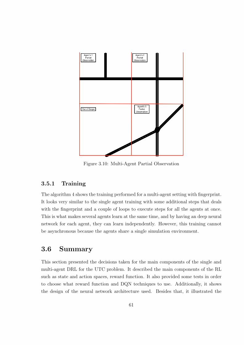
Figure 3.10: Multi-Agent Partial Observation
3.5.1 Training
The algorithm 4 shows the training performed for a multi-agent setting with fingerprint.
It looks very similar to the single agent training with some additional steps that deals
with the fingerprint and a couple of loops to execute steps for all the agents at once.
This is what makes several agents learn at the same time, and by having an deep neural
network for each agent, they can learn independently. However, this training cannot
be asynchronous because the agents share a single simulation environment.
3.6 Summary
This section presented the decisions taken for the main components of the single and
multi-agent DRL for the UTC problem. It described the main components of the RL
such as state and action spaces, reward function. It also provided some tests in order
to choose what reward function and DQN techniques to use. Additionally, it shows
the design of the neural network architecture used. Besides that, it illustrated the
61

Algorithm 4: Independent DDQN with Prioritized Experience Replay for Het-erogeneous Multi-Agent Training on Traffic Lights
Input: replay buffer size M, minibatch size B, greedy ε, learning rate α, learningfrequency λ, times steps T, target network update C, prioritized replayparameters pα and pβ, pre-train steps pt
Initialize simulator with time steps TInitialize optimizer with learning rate αInitialize agents AInitialize action-value function Q with random weights for each agent AInitialize replay memory D to capacity N and parameters pα, pβ and pε foreach agent A
Initialize target action-value function Q with weights θ− = θ for each agent A;for timestep = 1, T do
for agent = a, A doWith probability ε select a random action uatotherwise select uat = arg maxuQ(sat ,u;θa)Execute action uat in simulator
Get global reward rtfor agent = a, A do
Observe partial state sat+1
Add fingerprint to partial state sat+1
Store transition (sat ,uat ,rt,s
at+1) in Da
Update sat ← sat+1
if t > pt and t ≡ 0 mod λ thenSample minibatch of transitions (saj ,u
aj ,rj,s
aj+1) from Da based on
prioritiesMinimize the error in Bellman’s equation and compute TD-error δajUpdate the priorities in the replay buffer Da with TD-error δaj
Every C steps reset Qa = Qa
62

training algorithm for both, single and multi-agent environments. The next chapter
will presents how we implemented these components.
63
Chapter 4
Implementation
This chapter describes the implementation of the multi-agent DRL system and the
UTC simulation environment. We introduce the OpenAI’s baseline framework [39]
that we used to implement the DRL agents. We describe the implementation of DRL
agents and the communication between agents and the simulation environment.
4.1 Simulation Environment
The simulation environment used for the experiments is SUMO [40]. SUMO is an open
source, highly portable, microscopic and continuous road traffic simulation package
designed to handle large road networks. We use the Python API so-called TraCI in
order interact with the simulator. This interface allows modifying and getting access
to components such as traffic lights and vehicles, thus we set the phases of the traffic
light according to the action chosen by the agent through this API. Besides that, this
interface allow us to recover metrics of the environment such as position and speed
of the vehicle in order to build up the state matrices, as well as the variables used
for the reward function. One of the variables used as part of the reward function is
the waiting time. The waiting time for a vehicle is defined by SUMO as the time (in
seconds) spent with a speed below 0.1 m/s since the last time it was faster than 0.1 m/s.
One simulated second in SUMO is equal to one time step. We use the accumulated
waiting time function of TraCI in order to collects the waiting time of every vehicle
over a certain time interval which in this case is the whole simulation time.
64
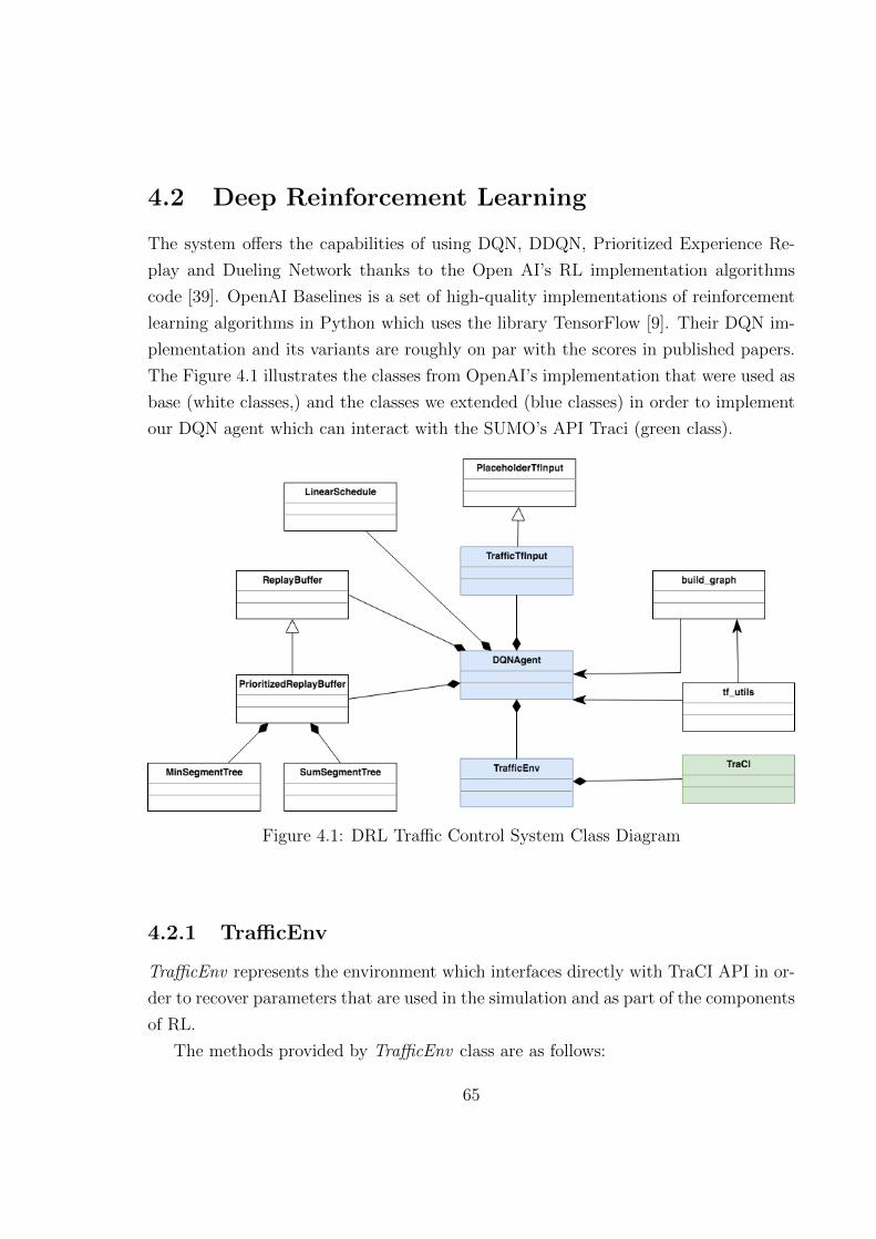
4.2 Deep Reinforcement Learning
The system offers the capabilities of using DQN, DDQN, Prioritized Experience Re-
play and Dueling Network thanks to the Open AI’s RL implementation algorithms
code [39]. OpenAI Baselines is a set of high-quality implementations of reinforcement
learning algorithms in Python which uses the library TensorFlow [9]. Their DQN im-
plementation and its variants are roughly on par with the scores in published papers.
The Figure 4.1 illustrates the classes from OpenAI’s implementation that were used as
base (white classes,) and the classes we extended (blue classes) in order to implement
our DQN agent which can interact with the SUMO’s API Traci (green class).
Figure 4.1: DRL Traffic Control System Class Diagram
4.2.1 TrafficEnv
TrafficEnv represents the environment which interfaces directly with TraCI API in or-
der to recover parameters that are used in the simulation and as part of the components
of RL.
The methods provided by TrafficEnv class are as follows:
65
• generate route file(self), which generates the traffic for all the road network
for each simulation based on a uniform distribution.
• get next observation(self), which gets transitions to the next step in the
simulation and build the state matrices for the new state.
• get reward(self), which returns the reward for the current transition.
• reset(self), which restarts all the settings of the simulation in order to start a
new episode.
• step(self, action), which takes an action at and transitions from st to the new
state st+1. This method returns the new states+1, the reward rt and a boolean
flag indicating if the episode or simulation have finished.
4.2.2 TrafficTfInput
TrafficTfInput works as a wrapper of a regular tensorflow placeholder. The main dif-
ferences are: (1) it possibly uses multiple placeholders internally and returns multiple
values and (2) it can apply light postprocessing to the value feed to placeholder. It
receives as parameters the shape of the tensor and the name of the underlying place-
holder. In our implementation this class wraps the observation of the environment
which is the state matrices that are the image-like representation of the environment.
4.2.3 DQNAgent
DQNAgent is the agent which interacts with the environment through the class Traf-
ficEnv and uses the implementation of the DRL algorithms from the different OpenAI
baseline’s classes. It implements the DQN-learning process by executing the Algorithm
3 of Chapter 4. Besides that, it builds the Convolutional Neural Network shows in 3.9
in Chapter 4. It allows to enable and disable the DRL techniques: DDQN, Prioritized
Experience Learning, Experience Replay and Dueling Network.
The DQN Agent requires the following parameters:
• simulation time st.
• pre-train pt.
66

• learning rate α.
• discount factor γ.
• minibatch size B.
• replay buffer size M.
• learning frequency λ.
• target network update C.
• prioritized experience replay parameters pα and pβ.
The methods provided by DQNAgent class are as follows:
• model(img in, num actions, scope), which creates a tensorflow graph with 3
CNN and 2 fully connected layers.
• dueling model(img in, num actions, scope, reuse=False), which creates a ten-
sorflow graph with 3 CNN and 2 fully connected layers for actions and state pairs
to create a dueling network.
• take action(self, t), which takes action and updates exploration ε-greedy value.
• store(self, rew, new obs, done), which stores the tuple <obs, rew, new obs, ac-
tion, done> into the replay buffer.
• learn(self, t), which minimizes the error in Bellman’s equation on a batch sam-
pled from replay buffer and compute TD-error.
• update target network(self, t), which updates the target network.
4.3 Neural Network Architecture
The architecture was build on top of the implementation of OpenAI baseline which
uses TensorFlow to program Neural Networks.
The Figure 4.2 shows the implementation in TensorFlow of the Dueling Network as
specified in the Figure 3.9. It consists of 3 convolutional neural networks followed by 2
67
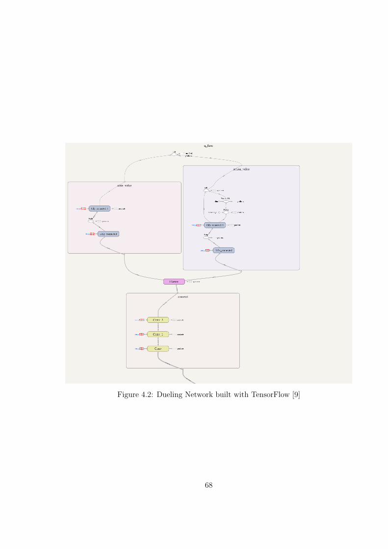
Figure 4.2: Dueling Network built with TensorFlow [9]
68

fully-connected layers that both has an advantage (i.e. state value) and an action (i.e.
action value) streams.
Figure 4.3: Deep Q-Networks built with TensorFlow [9]
The Figure 4.3 shows the implementation in TensorFlow of the two Deep Q-Network
used for Deep Q-Learning. The Neural Network in the left is the primary network θ,
while the one in the right is the target network θ− which is updated periodically with
the weights of the primary network θ every C steps. Both networks are identical, and
they share the same aforementioned architecture specified in the Figures 3.9 and 4.2.
Finally, the Figure A.2(the figure was placed in the appendix section in order to
show the image as bigger as possible) describes the whole Neural Network infrastruc-
ture build in TensorFlow. It presents a holistic view of the Neural Network and the
interactions between the main components. All the components are collapsed in order
to show a summary view of the main components. The main components present in
the illustrations are:
• Primary Network represented as ”q func”.
• Target Network represented as ”target q func”
• Double DQN is represented in the output of ”q func 1” through the usage of the
”ArgMax”, ”one hot 1” and reduction of ”Sum” TensorFlow’s operations which
work as input for the selection and evaluation of the Q-values.
• ADAM Optimizer represented as ”Adam” with gradient (i.e. gradient descent)
and beta 1 power (i.e. β1) and beta 2 power (i.e. β2) as inputs.
69

4.3.1 Optimizer
This subsection intends to analyse the experiments done in order to select the op-
timizer that performs better between the two most popular optimizers used in the
previous works, namely RMSProp and ADAM. The evaluation were executed with
hyper-parameters show in Table 4.1
Table 4.1: Reward function evaluation hyper-parameters
Parameter Value
Episodes 1000Time steps 3600000Pre train time steps 2500learning rate 0.0004Exploration ε 1.0 → 0.01Time steps from starting ε to ending ε 360000Target network update 5000Prioritization exponent α 0.6Prioritization importance sampling β 0.4 → 1.0Discount factor γ 0.99Replay Memory size M 50000Minibatch size B 32
Firstly, the figure 4.4a shows how ADAM starts getting higher rewards around 200
episodes. At around 400 episodes, ADAM outperforms RMSProp by 200%. After 600
episodes RMSProp starts getting higher results, however it stills under the performance
of ADAM which reaches around 100% more rewards.
Secondly, the figure 4.4b presents results that are correlated with the rewards since
from figure 4.4a can be noticed how bigger rewards result on lower average waiting
times. When ADAM starts getting better rewards at around 400 episodes, the average
waiting time is also decreased outperforming by ∼ %800 the RMSProp method. The
same behaviour happens with RMSProp when it starts getting larger rewards, the
average waiting time is reduced by ∼ %900 from episodes 400-600 to episodes 600-900.
Lastly, the figure 4.4c show a huge difference in the average travel time across the
whole training.
70

(a) Cumulative Reward per Episode
(b) Average Waiting Time per Episode (c) Average Travel Time per Episode
Figure 4.4: Comparison between RMSProp and Adam Optimizers
71

4.4 Multi-Agent Deep Reinforcement Learning
The figure 4.5 illustrates the classes implemented for IDQN. This is an small extension
of what was showed in section 4.2. The only additon is the class IDQN (marked with
red), which is a orchestrator between the simulator environment managed by TrafficEnv
and the agents implemented on DQNAgent.
Figure 4.5: IDQN Traffic Control System Class Diagram
Also, some small extensions were applied to the other classes in order to support
the IDQN.
4.4.1 TrafficEnv
The following methods were added:
• set phase(self, action, traffic light id, actions), which executes the action given
by the index action in the actions vector in the intersection with identifier traf-
72

fic light id. it is also responsible to introduce yellow lights if the phase is changed
from the previous state.
• make step(self), executes an step in the simulator, i.e. advances from st to st+1.
4.4.2 DQNAgent
The following methods were added:
• add fingerprint to obs(self, obs, weights, identifier, td errors), which adds the
weights and the td errors vector to the obs in the column identifier. Normally
used to add the fingerprint to the new observation of st1 .
• add fingerprint(self, weights, identifier, td errors), which encapsulates the pre-
vious method add fingerprint to obs with the current observation, i.e. state st.
4.5 IDQN Neural Network
Figure 4.6: Independent Deep Q-Networks for 3 agents built with TensorFlow [9]
The figure 4.6 shows the implementation of the IDQN for three agents. Every one
of these agents possesses one exact copy of the neural network described earlier in 4.3
and in A.3. The Tensor deep0 1 and deep0 are the neural networks of the intersection
73

with identifier 0 in the simulation, the same nomenclature is applied to the tensors of
intersections with identifiers 5 and 8.
4.6 Summary
In this chapter we have presented the implementation of DRL agents as defined by the
algorithm in Chapter 4. We also have presented the OpenAI Baseline code that we
used to implement the DRL agents. We have presented extensions to the framework we
have implemented in order to enable the development of Traffic Light DRL agents with
capability of interacting with the traffic simulator SUMO. We have then presented the
implementation in TensorFlow of the Deep Q Neural Network Architecture defined in
Chapter 4. Finally, we described how the implementation was extended for the classes
involved as for the Neural Networks in order to accomplish the IDQN technique.
74

Chapter 5
Evaluation
In this section we present an evaluation of IDQN as solution for multi-agent DRL
for heterogeneous agents in traffic light control. We present the objectives of the
evaluation, along with hyperparameters of the system that we used to execute the
experiments. It also describes the metrics for measuring the performance of the system.
We describe the experiments we used for the evaluation, and present and analyze their
outcomes.
5.1 Objectives
The goal of the evaluation of IDQN presented in this chapter is to establish how well
IDQN addresses the non-stationarity in a heterogeneous multi-agent environment. The
main objective of the design of IDQN was to provide a decentralized and independent
heterogeneous multi-agent optimization technique that establishes IDQN as the tech-
nique for UTC when using DRL methods. In Chapter 3 and 5 we outlined how the
design and implementation of IDQN addresses the requirements for such a system,
however, the success of IDQN as a technique for heterogeneous multi-agent technique
depends on its performance in a variety of evaluation scenarios.
IDQN can be said to have succeeded in addressing the non-stationarity for hetero-
geneous multi-agent setting if it satisfies the following performance requirements:
• IDQN outperforms existing UTC optimization techniques which cannot manage
heterogeneous intersections. Note that we only consider stationary traffic con-
75

ditions, as, once a suitable behaviour for that set of conditions has been learnt,
IDQN does not have the ability to adapt to a change in traffic pattern. Pattern
change detection and adaptation to new patterns is a subject for future work (see
Chapter 6).
• IDQN enhances the performance of UTC systems under a variety of traffic con-
ditions (e.g. traffic load, traffic patterns).
• IDQN is not impacted for the non-stationarity of the environment caused during
independent training.
5.2 Metrics
The metrics are the same as the ones used for single agents. These are: Cumulative
Rewards, Average Waiting Time and Average Travel Time. Every metric is sampled
per episode. More about metrics can be found in section A.2.
5.3 Evaluation Scenarios
In this section we describe the scenarios that we used to evaluate the suitability of
IDQN for heterogeneous multi-agent system. We first present the techniques that are
going to be tested against IDQN. Then, we describe the different scenarios where these
techniques are going to run.
5.3.1 Evaluation Techniques
• Fixed Time / Round Robin (FT). This is a predefined configuration for all
the traffic lights where the duration and order of the phases is fixed and pre con-
figured. In our experiments every phase takes 60 time steps, which corresponds
to 1 simulated minute. The order of the phases is given by SUMO. Our agent
just makes the transition to the next phase. This technique also keeps the yellow
transition duration to avoid collisions.
• IDQN without experience replay (ERM Disabled). It is a IDQN tech-
nique but the experience replay is disabled, therefore the agent cannot store
76
experiences. This technique is tested to verify if the agent can learn without
memory. By disabling the experience replay, the agent cannot be impacted for
the non-stationarity because it is not basing its decisions on possible corrupted
experience replays records.
• IDQN with prioritized experience replay (PEMR). It is a normal IDQN
technique which uses the experience replay as recommended for DQN. This tech-
nique is a target to be influenced by the non-stationarity of the environment as
has been explained before.
• IDQN with prioritized experience replay and fingerprint (PEMR +
FP). This is the proposed IDQN technique with the fingerprint to disambiguate
the age of experience replays. This technique should not be influenced by the
non-stationarity of the environment as has been explained before.
• IDQN with standard experience replay (ERM). This is IDQN with the
standard experience replay, not with prioritized experience replay.
5.3.2 Scenarios
Every technique will tested in the following scenarios:
• Low traffic load. A scenario where the number of vehicles is reduced. It
represents a normal flow where is not peek time. However, it is a good amount
of cars to produce traffic jams if the traffic control is not good.
• High traffic load. A scenario where the number of vehicles is overwhelming. It
represents the traffic load in peek times. This scenario certainly will produced
long queues and traffic jams even with good control. The idea is to verify if it is
possible and how much can be reduced in such a overcrowded scenario.
Every technique will use the parameters and network layout defined in section 5.4.
5.4 Setup
This sections describes the environment where the experiments were run as well as the
different parameters and configurations chosen. We first introduce the network layout
77
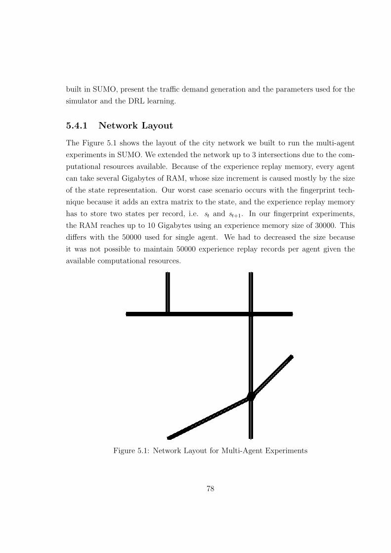
built in SUMO, present the traffic demand generation and the parameters used for the
simulator and the DRL learning.
5.4.1 Network Layout
The Figure 5.1 shows the layout of the city network we built to run the multi-agent
experiments in SUMO. We extended the network up to 3 intersections due to the com-
putational resources available. Because of the experience replay memory, every agent
can take several Gigabytes of RAM, whose size increment is caused mostly by the size
of the state representation. Our worst case scenario occurs with the fingerprint tech-
nique because it adds an extra matrix to the state, and the experience replay memory
has to store two states per record, i.e. st and st+1. In our fingerprint experiments,
the RAM reaches up to 10 Gigabytes using an experience memory size of 30000. This
differs with the 50000 used for single agent. We had to decreased the size because
it was not possible to maintain 50000 experience replay records per agent given the
available computational resources.
Figure 5.1: Network Layout for Multi-Agent Experiments
78

5.4.2 Traffic Demand
The demand traffic is generated with the algorithm 5 described in A.1. The traffic
demand generated for the multi-agent experiments set the values probability p = 0.1
for high load traffic and p = 0.05 for low traffic load. The time steps TS continues to
be 3600. As result, the expected number of vehicles in the simulation for high traffic
load is approximately 1900 to 2500 cars, and for low traffic load is approximately 1300
to 1600 cars, with departure times between 0 and 3600.
The Figure 5.2 shows the entry and departure points for the multi-agent experi-
ments. Every route is defined by specifying a source and a destination point (green
bullets), and one or more intersections (blue points) to pass through. For instance,
a simple route can be 6-5-0-2, and a longer and complicate route can be defined as
13-8-0-5-7. Therefore, routes with different lengths can be created.
Figure 5.2: Entry and Departure points in Network for Multi-Agent Experiments.Green points correspond to entry and departure points, while blue points are intersec-tions.
79

The routes created for our evaluation are the following:
• 6 → 5→ 0→ 2.
• 2 → 0→ 5→ 6.
• 4 → 0→ 8→ 10.
• 10 → 8→ 0→ 4.
• 13 → 8→ 9.
• 9 → 8→ 13.
• 4 → 0→ 5→ 7.
• 7 → 5→ 0→ 4.
• 13 → 8→ 0→ 2.
• 6 → 5→ 0→ 8→ 9.
5.4.3 Hyper-paraments
The table 5.1 describes the hype-parameters used for the multi-agent experiments.
They are the same hyper-parametes used for single-agents except for the Replay Mem-
ory size M, which had to be reduced due to the machine where the experiments were
carried out cannot support 3 concurrent agents with 50000 of memory. Every episode
corresponds to 1 hour of simulation time which is 3600 time steps, where every time
step is 1 simulated second.
5.5 Results and Analysis
In this section we analyse the performance of IDQN with respect to the evaluation
objectives outlined in section 5.1. We evaluate the efficiency of IDQN by comparing
against all the techniques mentioned in section 5.3.1 in two scenarios, high and low
traffic demand. We describe the results, analyse them and discuss how they relate to
the evaluation objectives.
80

Table 5.1: Multi-agent evaluation hyper-parameters
Parameter Value
Episodes 1000Time steps 3600000Pre train time steps 2500Learning rate 0.0004Exploration ε 1.0 → 0.01Time steps from starting ε to ending ε 360000Target network update 5000Prioritization exponent α 0.6Prioritization importance sampling β 0.4 → 1.0Discount factor γ 0.99Replay Memory size M 30000Minibatch size B 32
5.5.1 Low Traffic Load
In this section we compare the performance of IDQN with 3 different techniques, i.e.
EMR Disabled, PEMR and PEMR + FP. Also, a baseline FT is added. As extra exper-
iment, a standard experience replay (ERM) was used to validate the results obtained
with prioritized experience replay in previous experiments. The Figure 5.3 presents
the set of experiments that we carried out in a low traffic load setup.
Figure 5.3a shows the cumulative reward obtained per episode for the 4 techniques.
FT gets a constant reward range that varies extremely low around 50. This is because
this techniques does not adjust its performance, and the variation are a product of the
discrepancy of the traffic generation from episode to episode. From this results, we
can notice that disabling the experience replay (EMR Disabled) gets very bad rewards,
even worse than the baseline, and it never learns. Therefore, disabling the experience
replay is not useful for our UTC problem. Finally, we compare the results of the two
more promising techniques, i.e. PERM and PERM + FP, out of the four presented.
The results shows the both techniques have identical performance getting 400% bigger
rewards than FT. They also learn very well in spite of the non-stationarity, increasing
the rewards from around 25-100 in the exploration phase up to around 200-250 in
the exploitation phase. They reach their optimal point at 300 episodes, where they
get to keep a stable rewarding. Based on this similarity on the results of PEMR and
81

PEMR + FP, we deduce that the fingerprint is not helping to get bigger rewards. We
analyse the other metrics, and based on that, we conclude why FP is not enhancing
the performance.
In terms of waiting time, as expected FT, similarly that in rewards, gets a con-
stant behaviour that varies proportionally to the number of cars generated from each
episode. In the case of the EMR Disabled, it shows the direct result of getting very
bad rewards which produces extremely high waiting times (results cut in 2000 ms as
maximum in order to show the other results in a visible comparable scale). Then, again
PEMR and PEMR + FP get alike performance, with very low waiting times which are
approximately 300% less than FT, with some episodes with peeks higher than this
baseline. From these results we can also conclude that the fingerprinting is not helping
to enhance the system.
Finally, in the average travel time, EMR Disabling continues getting extremely poor
results in comparison to other techniques. We also notice that FT, PEMR and PEMR
+ FP gets similar performance by achieving travel times of around 100 ms. This is
because this metric is not proper for the multi-agent setting because there are routes
with different lengths, some are very long routes and others are very short routes. This
metric worked for single agent because in that case all the routes had the same length.
This metric should change to an average travel time per route, but if there are many
routes another approach needs to be taken. It is frequent to see the average time of a
service reported (Strictly speaking, the term average does not refer to any particular
formula, but in practice it is understood as the arithmetic mean: given n values, add
up all the values, and divide by n). Nonetheless, the mean is not a good metric if the
”typical” time of a service wants to be known, because it does not indicate how many
cases actually experienced that time. Normally it is better to use percentiles. If a list
of times is taken and sorted from fastest to slowest, the median is the middle point.
For instance, if the median time is 100 ms, that means half of the vehicles travelled
in less than 100 ms, and half of them took them longer than 100 ms. This makes the
median a good metric to know how long vehicles typically take to travel. The median
is also known as the 50th percentile, and sometimes abbreviated as p50. All in all, we
are not analysing this measurement because it does not make sense for our multi-agent
setting.
Now, we move to analyse why the fingerprint is not making better the traffic light
82

(a) Cumulative Rewards per Episode
(b) Average Waiting Time per Episode
(c) Average Travel Time per Episode
Figure 5.3: Low Traffic IDQN Experiments
83
control. Our hypothesis holds two possible reasons:
• The components we chose for the fingerprint are not good, because they do not
correlate enough with the true value of state-action pairs given the other agents’
policies and/or it does not vary smoothly over training, which does not to allow
the model to generalise across experiences in which the other agents execute
policies as they learn. Likely another component of the DQN training should be
used as fingerprint.
• The prioritized experience replay is good enough to deal with the non-stationarity
because of main components such as the importance weights it uses to know
what records are more valuable samples. This weighting could be enough to
disambiguate the age of the data.
Of course, we should run more tests to prove if these hypothesis are true. Because
of the long time these experiments take to run, we only tried to verify the second
point by executing a test with a standard experience replay. The figure 5.4 shows this
additional experiment which compares the standard experience replay (EMR) against
our proposed fingerprint technique with Prioritized Experience Replay (PEMR + FP)
which gets an identical performance than Prioritized Experience Replay without fin-
gerprint (PEMR).
As shown in Figure 5.4a, both techniques, EMR and PEMR + FP, learn well, but
PEMR + FP obtains higher rewards outperforming ERM in around 45% in the highest
point of PEMR + PR when it gets rewards between 150 and 250 while EMR is getting
rewards ranging from 100 to 170. In the case of waiting time illustrated in 5.4b, they get
a similar performance, but EMR is more stable than PEMR + FP by not producing
peeks. As mentioned before, we ignore the average travel time because it is not a
good metric for the multi-agent setting. Regardless of the waiting time, we conclude
the Prioritized Experience Replay helps to deal with the non-stationarity by getting
bigger rewards, which indicates that PEMR has better performance than EMR. We can
minimize the importance of the waiting time results because they are a direct result
of the reward function, and PEMR is getting better results from the reward function
which is what the agent is going to look for. If by getting bigger rewards the waiting
time is not decreasing proportionally, it is a problem with the reward function that
84

(a) Cumulative Rewards per Episode
(b) Average Waiting Time per Episode
(c) Average Travel Time per Episode
Figure 5.4: Low Traffic IDQN Experiments with Standard ERM
85

do not correlate that strong with changes in the waiting time, and not a performance
problem of the technique. These results prove our second hypothesis that PEMR
can be good enough to deal with the non-stationarity. However, we cannot discard
the enhancement that fingerprinting can add to PEMR by selecting more appropriate
fingerprint components, and therefore, verifying if the first hypothesis is also true.
Although, due to time constraint we are not able to demonstrate the first hypothesis.
5.5.2 High Traffic Load
In this section we compare the performance of IDQN with 3 different techniques, i.e.
EMR Disabled, PEMR and PEMR + FP. Also, a baseline FT is added. The Figure
5.5 presents the set of experiments that we carried out in a high traffic load setup.
The Figure 5.5a illustrates the results for the cumulative rewards per episode. As
can be seen, FT makes a good job in this scenario along with PEMR, both outperforms
EMR Disabled and PEMR + FP in around 25%. It seems that the extra layer of
the fingerprint reduces the performance of the technique under intense traffic loads.
Moreover, none DRL technique gets to learn over the episodes, the performance is
constant across all the training. This can indicate that the agents needs more training
for such a high load. If we compare the rewarding pattern in Figure 5.3a, we notice
that all the DRL techniques are below FT before episode 100, but after it all PEMR
and PEMR + FP beat FT, and EMR Disabled becomes worse. This behaviour might
happen after more training episodes in high load. This bad performance in learning can
be also produced by a short exploration time, the e-greedy parameter can be increased
to allow a more extend exploration of the states.
In terms of the average waiting time, the results are similar to the low traffic load
on which techniques perform better. EMR Disabled gets very poor results with a
huge magnitude of difference in comparison to all the other techniques. Then, FT
gets constant average waiting times as expected reaching around 100% higher times.
PEMR and PEMR + FP are the technique which reach lowest waiting times with a
similar pattern of results, however PEMR + FP outperform slightly PERM. Alike the
reward results, there is not learning across the training.
We ignore the average waiting time as it does not make sense for multi-agent setting
as explained in the previous section.
86

(a) Cumulative Rewards per Episode
(b) Average Waiting Time per Episode
(c) Average Travel Time per Episode
Figure 5.5: High Traffic IDQN Experiments
87
5.6 Evaluation Summary
In this chapter we presented details of the evaluation of IDQN as a heterogeneous
DRL multi-agent technique. We have presented the evaluation objectives, described
the evaluation scenarios, the setup of the environment and presented and analysed the
results.
From the analysis of the results we conclude that IDQN is a suitable algorithm
for heterogeneous multi-agent UTC, and as such could be a promising approach to
optimization in other large-scale decentralized autonomic systems with similar char-
acteristics. However, the addition of the fingerprint is not helping the performance
of IDQN. It seems the Prioritized Experience Replay can deal better than a standard
Experience Replay with the non-stationarity of the environment. Although, the three
techniques achieve a good learning and performance, but it might be improve with a
better choice of a fingerprint.
IDQN outperforms the baseline (FT) and the existing multi-agent UTC techniques
by dealing with heterogeneous agents, and therefore, with the non-stationarity of the
environment (Objectives #1 and #3 as listed in section 5.1). IDQN enhances the
performance of UTC systems by managing adequately heterogeneous intersections in
low traffic load. Nevertheless, the high traffic load can need adjustments in the hyper-
parameters in order to get optimal results. Also, the IDQN with fingerprint we chose
is not improving the performance of the technique without it (Objective #2 as listed
in section 5.1).
88

Chapter 6
Conclusions and Future Work
In this chapter we summarize the thesis and review its most significant achievements.
We then conclude with a discussion of the remaining open research issues related to
this work.
6.1 Thesis Contribution
This thesis is the only recent work which addresses heterogeneous multi-agent DRL in
UTC systems.
Chapter 1 motivated the work by outlining issues in multi-agent optimization in
UTC systems. We argued that the main challenges in such systems arise from the
heterogeneity and dependency of agents caused by shared operating environments.
Due to these dependencies, we concluded that cooperation between agents could be
beneficial, however, we have identified that collaboration introduces further issues, for
example, with what other agents should they cooperate, how the changing environment
can affect the training of the agents (non-stationarity).
Chapter 2 gave the background material used to design and implement IDQN.
It covers RL and DRL techniques. Specifically, we describe the RL framework, the
operation of DL, the aggregated DRL techniques, IQL and the proposed fingerprint
method. In addition, it presented the more recent work in MARL, and single and
multi-agent DRL. This related work investigation showed that none study has tried
to work with heterogeneous network layouts because of the non-stationarity of the
89
environment.
Chapter 3 describes the design decisions taken to build the IDQN techniques. It
presented some experiments to back up the different design choices. Particularly, it
covered the RL components (i.e. state, actions and reward function), the neural net-
work design, the selection of the adequate DRL techniques, and the algorithms for
single and multi-agent settings.
Chapter 4 presented details of the implementation of IDQN for single and multi-
agents scenarios. This includes a brief review of the code, the implementation of the
neural network in TensorFlow, and the frameworks used for the simulator and the
DRL, SUMO and OpenAI baselines respectively.
Chapter 5 evaluated IDQN as a heterogeneous multi-agent DRL method for UTC
systems by using SUMO. We evaluated IDQN’s performance with different configura-
tions, i.e. without experience replay, with experience replay and with experience replay
with fingerprint. We compared against a baseline which uses a round robin approach.
We executed test in two traffic conditions, with low and high traffic loads. Our exper-
iments shows the IDQN is a suitable techniques for heterogeneous multi-agent UTC
environments which can deal with the non-stationarity of the environment. The best
results were obtained in the low traffic load. The high traffic load seems to need longer
training time. From the successful experiments, we proved the IDQN outperforms the
baseline and the experience replay is mandatory to learn efficiently. Nonetheless, the
fingerprint we chose do not add any performance enhancement over the normal priori-
tized experience replay. Both gets identical performance. We also demonstrated that
prioritized experience replay outperforms the standard experience replay in around
45% for the rewards.
6.2 Future Work
When designing and evaluating IDQN, we identified several areas where IDQN’s per-
formance and applicability could be extended and identified a number of areas for
potential future research. We outline these areas and discuss the remaining open re-
search issues below.
• New fingerprint: The fingerprint that consists of the prioritized experience
90

replay’s weights and the TD-Error does not improve the performance. Thus,
it needs further investigation and experimentation in order to find out better
components as candidates for fingerprint. Also, the way of how we integrate the
fingerprint as an additional matrix can be carefully studied to verify if it is the
best manner to add the fingerprint in a system the uses a image-like representation
as the state of the RL system.
• Aggregated DRL techniques: Use more aggregated DRL techniques that can
improve the performance of IDQN as was applied in Atari games in [24], such as
Multi-step learning, Distributional RL and Noisy Nets which ends creating the
Rainbow technique which is the current state-of-the-art DRL technique.
• Homogeneous intersection experimentation: Test IDQN’s performance in
a homogeneous multi-agent environment to validate whether it holds the same
performance as with heterogeneous multi-agent setting or it increases that per-
formance, and therefore, if it deals with the non-stationarity of a homogeneous
setting. This should be an easy verification as a homogeneous environment is a
simpler/trivial case of a heterogeneous environment.
• Scale multi-agent training with distributed computation: Place every
agent with its deep neural network in a different computer or node, and the
shared simulator in a different computer or node which interacts with all the
agents in a distributed manner. The purpose of a distributed system is to scale
the training to more than 3 agents by using several machines (Horizontal Scaling)
and not be limited by the computational resources of only one machine (Vertical
Scaling).
• Multi policy DRL: Extend the work to support multi policies with multi-
agents; for instance, special vehicles prioritization. [41] uses HER to achieve a
multi policy DRL.
• Different Demand Traffic Generation: The traffic demand generation used
follows a uniform distribution. However, in the real world the traffic demand
changes from different hour; i.e. it is higher in rush hours and lower at other
times, and different routes may have different demand distribution. A suitable
approach could be use real world street network and data.
91
• Longer Training Times We used 1000 episodes for all the experiments, however
the studies normally use 1600 to 2000 episodes of training. We use 1000 episodes
due to time constraints of the research. For example, the experiments of high load
traffic obtained suboptimal results that could have been caused by the limited
training time. Maybe some results would change significantly if they had had
more longer training times.
• Real images as state representations: Instead of using pre-processed image-
like matrices state representations, the system can use direct snapshots of the GUI
simulator. This helps to increase the flexibility of the system by eliminating things
like fixed cells to locate vehicles. Also, images can provide more information to
the agent. This can mean a change in some layers of the neural network.
• Pattern change detection and adaptation: IDQN could detect fluctuations
in the traffic flow and adapt its behaviour to those variations by changing the
policy somehow.
92

Appendix A
Appendix
A.1 Traffic Demand Generation
The cars for every simulation are auto generated. Each vehicle has a predefined route
which follows a list of connected edges with the source and destination points that a
vehicle must follow. This pre-configuration is defined in a demand XML configuration
file which is auto-generated by using the Algorithm 5. Every vehicle in SUMO consists
of three parts: (1) a vehicle type which describes the vehicle’s physical properties, (2)
a route the vehicle must follow and (3) the vehicle itself. Both routes and vehicle types
can be shared by several vehicles. It is not mandatory to define a vehicle type. If not
given, a default type is used.
Demand data is auto generated for both the single and multiple intersections using
Algorithm 5. It uses a uniform distribution to generate cars for all the routes.
The vehicle’s parameters work as follows:
• maxSpeed. The vehicle’s maximum velocity (in m/s).
• accel. The acceleration ability of vehicles of this type (in m/s2).
• decel. The deceleration ability of vehicles of this type (in m/s2).
• minGap. Empty space after leader [m].
• sigma. The driver imperfection (between 0 and 1).
93
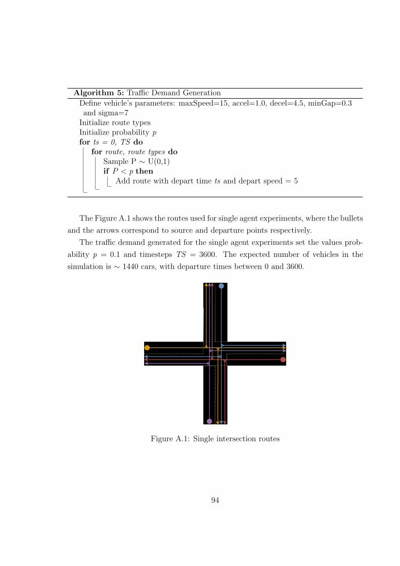
Algorithm 5: Traffic Demand Generation
Define vehicle’s parameters: maxSpeed=15, accel=1.0, decel=4.5, minGap=0.3and sigma=7
Initialize route typesInitialize probability pfor ts = 0, TS do
for route, route types doSample P ∼ U(0,1)if P < p then
Add route with depart time ts and depart speed = 5
The Figure A.1 shows the routes used for single agent experiments, where the bullets
and the arrows correspond to source and departure points respectively.
The traffic demand generated for the single agent experiments set the values prob-
ability p = 0.1 and timesteps TS = 3600. The expected number of vehicles in the
simulation is ∼ 1440 cars, with departure times between 0 and 3600.
Figure A.1: Single intersection routes
94
A.2 Metrics for Experiments
We select 3 metrics that have been used in several DRL studies for UTC. These metrics
are taken for single and multi-agent experiments. Every metric is taken per episode.
A episode consists of 3600 time steps, and each time step is 1 simulated second. The
metrics are the following:
• Cumulative Reward. It is the most common metric for RL experiments due
to the performance of the algorithms is directly related with how many rewards
the agent can collect over the long time. The agent must collect as many rewards
as possible. Bigger numbers means better performance. The reward rt taken on
every time step t is accumulated until the episode is finished. This cumulation
reward scalar value is shown for every episode in the results.
• Average Waiting Time. This metric measures the effectiveness of the reward
function into the main goal of the system, which is to reduce the waiting time
of every driver in the traffic network. This metric is taken for every ith vehicle
that has updated its waiting time wit in the current time step t. Then, the sum
of all vehicles’ waiting time is the cumulative waiting time Wt at the time step
t. When the episode finishes, the sum of all the cumulative waiting time of every
time step, from 0 until 3600, is divided by 3600 in order to get the average of the
waiting time during an episode as shown in Equation A.1. The waiting time in
SUMO is defined in section 4.1. The waiting time is part of the reward function,
therefore this metric is correlated with the rewards of every episode.
AWT =Wt
3600(A.1)
• Average Travel Time. This metric is taken in the same way as the average
waiting time. On every time step t, new loaded vehicles in the network are
registered in a dictionary T with the timestamp of the time step when they enter
to the network as lt. Also, on every time step t, the loaded timestap of every
vehicle that departures the network is obtained from the dictionary T in order to
calculate the travel time of such vehicle. Therefore, the ith vehicle’s travel time
trit is calculated as the difference of the loaded time lt and the departure time dt
95

as shown in Equation A.2.
trit = dt − lt (A.2)
Similarly to the average waiting time, the sum of all vehicles’ travel time is the
cumulative travel time Tr. When the episode finishes, the cumulative travel time
is divided by the number of vehicles registered in the dictionary T in order to get
the average travel time of drivers during an episode as shown in Equation A.3.
Tr =
∑i
trit
|T |(A.3)
A.3 Complete views of the Implementation of the
Deep Neural Network
Figure A.2: Whole view of the Neural Network Architecture built with TensorFlow [9]
96
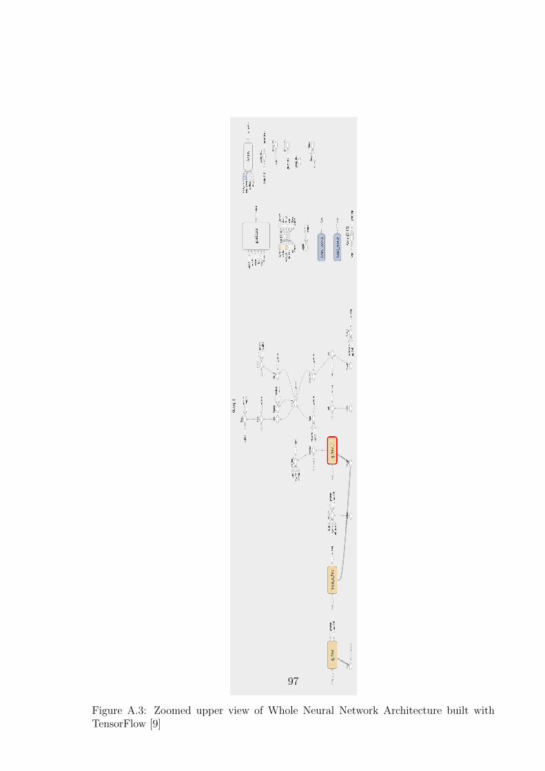
Figure A.3: Zoomed upper view of Whole Neural Network Architecture built withTensorFlow [9]
97

Figure A.4: Zoomed lower view of Whole Neural Network Architecture built withTensorFlow [9]
98

Bibliography
[1] Richard S. Sutton and Andrew G. Barto, Reinforcement Learning, Second Edition
An Introduction. MIT Press, second edi ed., 2018.
[2] Z. Wang, N. de Freitas, and M. Lanctot, “Dueling Network Architectures for Deep
Reinforcement Learning,” arXiv, no. 9, pp. 1–16, 2016.
[3] I. Dusparic and V. Cahill, “Autonomic multi-policy optimization in pervasive
systems,” ACM Transactions on Autonomous and Adaptive Systems, 2012.
[4] M. Tahifa, J. Boumhidi, and A. Yahyaouy, “Swarm reinforcement learning for traf-
fic signal control based on cooperative multi-agent framework,” Intelligent Systems
and Computer Vision (ISCV), 2015, pp. 1–6, 2015.
[5] L. Li, Y. Lv, and F.-Y. Wang, “Traffic signal timing via deep reinforcement learn-
ing,” IEEE/CAA Journal of Automatica Sinica, vol. 3, no. 3, pp. 247–254, 2016.
[6] J. Gao, Y. Shen, J. Liu, M. Ito, and N. Shiratori, “Adaptive Traffic Signal Con-
trol: Deep Reinforcement Learning Algorithm with Experience Replay and Target
Network,” arXiv, pp. 1–10, 2017.
[7] X. Liang, X. Du, G. Wang, and Z. Han, “Deep Reinforcement Learning for Traffic
Light Control in Vehicular Networks,” Ieee Transactions on Vehicular Technology,
vol. 1, no. Xx, pp. 1–11, 2018.
[8] F. Belletti, D. Haziza, G. Gomes, and A. M. Bayen, “Expert Level Control of
Ramp Metering Based on Multi-Task Deep Reinforcement Learning,” IEEE Trans-
actions on Intelligent Transportation Systems, vol. 19, no. 4, pp. 1198–1207, 2018.
99

[9] M. Abadi, P. Barham, J. Chen, Z. Chen, A. Davis, J. Dean, M. Devin, S. Ghe-
mawat, G. Irving, M. Isard, M. Kudlur, J. Levenberg, R. Monga, S. Moore,
D. G. Murray, B. Steiner, P. Tucker, V. Vasudevan, P. Warden, M. Wicke, Y. Yu,
X. Zheng, and G. Brain, “TensorFlow: A System for Large-Scale Machine Learning
TensorFlow: A system for large-scale machine learning,” in 12th USENIX Sympo-
sium on Operating Systems Design and Implementation (OSDI ’16), pp. 265–284,
2016.
[10] D. Bernstein, R. Givan, and N. Immerman, “The complexity of decentralized
control of Markov decision processes,” Mathematics of operations research, vol. 27,
no. 4, pp. 819–840, 2002.
[11] D. V. Pynadath and M. Tambe, “The communicative multiagent team decision
problem: Analyzing teamwork theories and models,” Journal of Artificial Intelli-
gence Research, vol. 16, pp. 389–423, 2002.
[12] J. K. Gupta, M. Egorov, and M. Kochenderfer, “Cooperative Multi-Agent Con-
trol Using Deep Reinforcement Learning,” Adaptive Learning Agents (ALA) 2017,
2017.
[13] J. Schulman, S. Levine, P. Moritz, M. Jordan, and P. Abeel, “Trust region policy
optimisation,” ICML, 2015.
[14] J. N. Foerster, N. Nardelli, G. Farquhar, P. H. S. Torr, P. Kohli, and S. Whiteson,
“Stabilising Experience Replay for Deep Multi-Agent Reinforcement Learning,”
CoRR, vol. abs/1702.0, 2017.
[15] J. Rosenschein and G. Zlotkin, “Designing conventions for automated negotia-
tion,” AI magazine, vol. 15, no. 3, pp. 29–46, 1994.
[16] M. L. Puterman, Markov Decision Processes: Discrete Stochastic Dynamic Pro-
gramming. New York, NY, USA: John Wiley & Sons, Inc., 1st ed., 1994.
[17] C. J. C. H. Watkins and P. Dayan, “Q-learning,” Machine Learning, vol. 8, no. 3-4,
pp. 279–292, 1992.
[18] I. Goodfellow, Y. Bengio, and A. Courville, Deep Learning. MIT Press, 2016.
100
[19] Y. A. LeCun, Y. Bengio, and G. E. Hinton, “Deep learning,” Nature, vol. 521,
no. 7553, pp. 436–444, 2015.
[20] Y. Duchi, John and Hazan, Elad and Singer, “Adaptive Subgradient Methods for
Online Learning and Stochastic Optimization,” The Journal of Machine Learning
Research, vol. 12, no. 1532-4435, pp. 2121–2159, 2011.
[21] G. E. Hinton, N. Srivastava, and K. Swersky, “Lecture 6a Overview of mini-batch
gradient descent,” 2012.
[22] D. P. Kingma and J. L. Ba, “Adam: a Method for Stochastic Optimization,”
International Conference on Learning Representations 2015, pp. 1–15, 2015.
[23] K. Arulkumaran, M. P. Deisenroth, M. Brundage, and A. A. Bharath, “Deep
reinforcement learning: A brief survey,” 2017.
[24] M. Hessel, J. Modayil, H. van Hasselt, T. Schaul, G. Ostrovski, W. Dabney,
D. Horgan, B. Piot, M. G. Azar, and D. Silver, “Rainbow: Combining Improve-
ments in Deep Reinforcement Learning,” CoRR, vol. abs/1710.0, 2017.
[25] V. Mnih, K. Kavukcuoglu, D. Silver, A. A. Rusu, J. Veness, M. G. Bellemare,
A. Graves, M. Riedmiller, A. K. Fidjeland, G. Ostrovski, S. Petersen, C. Beat-
tie, A. Sadik, I. Antonoglou, H. King, D. Kumaran, D. Wierstra, S. Legg, and
D. Hassabis, “Human-level control through deep reinforcement learning,” Nature,
vol. 518, no. 7540, pp. 529–533, 2015.
[26] H. V. Hasselt, A. C. Group, and C. Wiskunde, “Double Q-learning,” Nips, pp. 1–9,
2010.
[27] H. van Hasselt, A. Guez, and D. Silver, “Deep Reinforcement Learning with Dou-
ble Q-Learning,” in Proceedings of the Thirtieth AAAI Conference on Artificial
Intelligence, AAAI’16, pp. 2094–2100, AAAI Press, 2016.
[28] V. Mnih, K. Kavukcuoglu, D. Silver, A. A. Rusu, J. Veness, M. G. Bellemare,
A. Graves, M. Riedmiller, A. K. Fidjeland, G. Ostrovski, S. Petersen, C. Beattie,
A. Sadik, I. Antonoglou, H. King, D. Kumaran, D. Wierstra, S. Legg, D. Has-
sabis, H. van Hasselt, A. Guez, D. Silver, I. Sorokin, A. Seleznev, M. Pavlov,
101
A. Fedorov, A. Ignateva, D. Silver, A. Huang, C. J. Maddison, A. Guez,
L. Sifre, G. van den Driessche, J. Schrittwieser, I. Antonoglou, V. Panneershel-
vam, M. Lanctot, S. Dieleman, D. Grewe, J. Nham, N. Kalchbrenner, I. Sutskever,
T. Lillicrap, M. Leach, K. Kavukcuoglu, T. Graepel, D. Hassabis, T. Schaul,
J. Quan, I. Antonoglou, D. Silver, A. A. Rusu, S. Gomez Colmenarejo, C. Gul-
cehre, G. Desjardins, J. Kirkpatrick, R. Pascanu, V. Mnih, K. Kavukcuoglu,
R. Hadsell, A. Radford, L. Metz, S. Chintala, H. F. Olafsdottir, C. Barry, A. B.
Saleem, D. Hassabis, H. J. Spiers, V. Mnih, K. Kavukcuoglu, D. Silver, A. Graves,
I. Antonoglou, D. Wierstra, M. Riedmiller, Q. V. Le, M. Ranzato, R. Monga,
M. Devin, K. Chen, G. S. Corrado, J. Dean, A. Y. Ng, V. Mnih, K. Kavukcuoglu,
D. Silver, A. A. Rusu, J. Veness, M. G. Bellemare, A. Graves, M. Riedmiller, A. K.
Fidjeland, G. Ostrovski, S. Petersen, C. Beattie, A. Sadik, I. Antonoglou, H. King,
D. Kumaran, D. Wierstra, S. Legg, D. Hassabis, H. F. Olafsdottir, C. Barry, A. B.
Saleem, D. Hassabis, H. J. Spiers, T. Schaul, J. Quan, I. Antonoglou, D. Silver,
A. A. Rusu, S. Gomez Colmenarejo, C. Gulcehre, G. Desjardins, J. Kirkpatrick,
R. Pascanu, V. Mnih, K. Kavukcuoglu, R. Hadsell, H. van Hasselt, A. Guez,
D. Silver, K. Gregor, I. Danihelka, A. Graves, D. Jimenez Rezende, D. Wierstra,
N. Kalchbrenner, I. Danihelka, A. Graves, S. Lange, T. Gabel, M. Riedmiller,
N. Kalchbrenner, I. Danihelka, A. Graves, K. Gregor, I. Danihelka, A. Graves,
D. Jimenez Rezende, and D. Wierstra, “Prioritized Experience Replay,” Interna-
tional Conference in Machine Learning, vol. 4, no. 7540, p. 14, 2015.
[29] M. Tan, “Multi-Agent Reinforcement Learning: Independent vs. Cooperative
Agents,” in Machine Learning Proceedings 1993, pp. 330–337, Morgan Kaufmann
Publishers Inc., 1993.
[30] A. Tampuu, T. Matiisen, D. Kodelja, I. Kuzovkin, K. Korjus, J. Aru, J. Aru, and
R. Vicente, “Multiagent Cooperation and Competition with Deep Reinforcement
Learning,” arXiv, pp. 1–12, 2015.
[31] J. N. Foerster, Y. M. Assael, N. de Freitas, and S. Whiteson, “Learning to Commu-
nicate with Deep Multi-Agent Reinforcement Learning,” CoRR, vol. abs/1605.0,
2016.
[32] T. Chu and J. Wang, “Traffic signal control by distributed Reinforcement Learning
102

with min-sum communication,” in 2017 American Control Conference (ACC),
pp. 5095–5100, 2017.
[33] S. El-Tantawy and B. Abdulhai, “Multi-Agent Reinforcement Learning for In-
tegrated Network of Adaptive Traffic Signal Controllers (MARLIN-ATSC),” in
2012 15th International IEEE Conference on Intelligent Transportation Systems,
pp. 319–326, 2012.
[34] M. L. Littman, “Markov games as a framework for multi-agent reinforcement
learning,” in Machine Learning Proceedings 1994, pp. 157–163, Morgan Kaufmann
Publishers Inc., 1994.
[35] B. Fan, Q. Pan, and H. Zhang, “A multi-agent coordination framework based on
Markov games,” in CSCWD 2004 - 8th International Conference on Computer
Supported Cooperative Work in Design - Proceedings, vol. 2, 2004.
[36] S. Mousavi, M. Schukat, and E. Howley, “Traffic light control using deep policy-
gradient and value-function-based reinforcement learning,” IET Intelligent Trans-
port Systems, vol. 11, no. 7, 2017.
[37] E. Van Der Pol and F. A. Oliehoek, “Coordinated Deep Reinforcement Learners
for Traffic Light Control,” NIPS’16 Workshop on Learning, Inference and Control
of Multi-Agent Systems, no. Nips, 2016.
[38] M. Liu, J. Deng, M. Xu, X. Zhang, and W. Wang, “Cooperative Deep Reinforce-
ment Learning for Traffic Signal Control,” 23rd ACM SIGKDD Conference on
Knowledge Discovery and Data Mining (KDD), Halifax 2017, 2017.
[39] P. Dhariwal, C. Hesse, O. Klimov, A. Nichol, M. Plappert, A. Rad-
ford, J. Schulman, S. Sidor, and Y. Wu, “OpenAI Baselines.”
\url{https://github.com/openai/baselines}, 2017.
[40] D. Krajzewicz, J. Erdmann, M. Behrisch, and L. Bieker, “Recent Development and
Applications of {SUMO - Simulation of Urban MObility},” International Journal
On Advances in Systems and Measurements, vol. 5, pp. 128–138, dec 2012.
103

[41] M. Andrychowicz, F. Wolski, A. Ray, J. Schneider, R. Fong, P. Welinder, B. Mc-
Grew, J. Tobin, P. Abbeel, and W. Zaremba, “Hindsight Experience Replay,”
CoRR, vol. abs/1707.0, 2017.
104