Hedonic Price Indexes for Housing AcrossRegions and Time: The Problem of

Substitution Bias

Robert J. Hill Daniel Melser

Department of Economics Moody’s Economy.Com

University of Graz Level 10, 1 O’Connell Street

Universitatsstrasse 15/F4 Sydney, NSW 2000

8010 Graz, Austria Australia

Email: robert.hill@uni-graz.at Email: DMelser@economy.com

Draft: 16 April 2008

Abstract: Panel hedonic comparisons of house prices can be made using the region-

time-dummy method. This method is a natural extension to a panel context of

the widely used time-dummy and region-dummy methods. We show that these

methods are all affected by substitution bias, which can seriously distort their results.

We propose an alternative approach that is free of substitution bias which builds

up panel comparisons from bilateral building blocks using the hedonic imputation

method. This approach is very flexible. We consider a number of variants on this

method, all of which are likely to be improvements on the unconstrained region-

time-dummy method. We illustrate our findings using data for 14 regions in Sydney

over a six year period. We find clear evidence of bias in the region-time-dummy

results as well as in simple average measures such as the median that fail to adjust

for quality change. For these reasons we favor the hedonic imputations approach.

(JEL: C43, E31, O47, R31)

Keywords: Hedonic regression; Quality adjustment; Housing; Price index; Substitu-

tion bias; Multilateral indexes

* Funding from the Australian Research Council Discovery Grant Program and Linkage Grant Pro-gram in collaboration with the Australian Bureau of Statistics is gratefully acknowledged.

** The views expressed in this paper are those of the authors and do not necessarily reflect thoseof Moody’s Economy.Com.

1 Introduction

Housing is probably the most important asset in an economy. Englund, Quigley and

Redfearn (1998, p. 172) estimate that it accounts for more than 50 percent of the U.S.

private capital stock and 30 percent of household expenditure. The housing market

can be volatile and subject to bubbles [see Ito and Iwaisako (1996), Goodhart (2001)

and Garino and Sarno (2004)]. Given the possibility of interactions between house

prices and consumption, the measurement of price movements in the housing market

is hence of critical importance to understanding the economy.

Existing house price indexes often simply measure the average or median price

of houses sold in a particular period. This approach is problematic since the mix of

houses sold could change quite significantly over time. Suppose that the proportion

of low quality houses sold in period t is much higher than in period t+1. The change

in the average sale price from period t to t + 1 will therefore overestimate the actual

change in house prices (perhaps dramatically so).

For a price index to be meaningful, it must compare the prices of equivalent

products from one period (region) to the next. This is particularly problematic in

the case of housing where no two houses are identical, and a number of years (or

decades) may elapse between sales of a particular house. One approach for dealing

with this problem in a temporal context is to restrict the comparison to repeat sales,

i.e., houses that are sold at least twice during the time interval covered by the data

set. The repeat-sale method was developed by Bailey, Muth and Nourse (1963) and

has since been extended by amongst others Shiller (1991, 1993), Englund, Quigley

and Redfearn (1998), and Dreiman and Pennington-Cross (2004). The repeat-sale

method has become the method of choice in the real-estate industry for measuring

housing market conditions. Although sophisticated, and a huge improvement on the

average price approach, this method still has weaknesses. First, it cannot be used

to construct spatial price indexes since the same house cannot sell in two different

locations. Second, it does not make maximum use of the available data since houses

1

that are sold only once during the time interval of interest are omitted. Admittedly,

the severity of this problem decreases as the length of the time interval increases since

this reduces the share of houses that are sold only once as a proportion of all houses

sold. Third, the results for earlier periods typically need to be revised as new data

become available. Fourth, there is no guarantee that a house sold in one period is

equivalent to the same house sold in a later period. This is because the house may

have depreciated due to wear and tear or been renovated or enlarged between sales.

In other words, the repeat-sales method does not guarantee that like is compared

with like. Fifth, if repeat-sale houses tend to differ from single-sale houses in the data

set in some respects (for example apartments may sell more frequently than houses),

and if they follow different price paths (e.g., apartment prices rise more slowly than

house prices) then the index may be biased (in this case upwards).1

The hedonic approach to price index construction has the potential to resolve

all these issues and hence significantly improve the quality of house price indexes.

The essential idea is to regress the price of a product (in our case a house) on its

characteristics. The estimated parameters on the characteristics can be interpreted

as shadow prices of the characteristics (or functions thereof) which can then be used to

construct an imputed price for each product as a function of its characteristics. This

allows price indexes to be constructed even when products cannot be matched from

one period or region to the next. This counterfactual aspect of hedonic models can be

controversial. In the context of computers, for example, if a new model had appeared

on the market earlier than it actually did, this could have changed the whole market

structure and hence the prices of the computers actually sold in this earlier period.

The hedonic model, therefore, is easier to interpret in situations where it can be

1Shiller (1993) shows how the repeat-sales method can be modified to allow for variations in the

average quality (e.g. size) of houses sold each period. This helps to address the fifth criticism. It

is also common in repeat-sales models to exclude repeat sales that occur within six months, on the

grounds that this signals that the house may have been renovated. Such rules of thumb, however,

will only partially address the fourth criticism.

2

reasonably assumed that the counterfactual scenarios, if they had actually occurred,

would not have had a significant effect on the existing market. This assumption

is decidedly more reasonable in the case of housing than it is for computers. For

example, if a house that sold in 2003 had instead been on the market in 2001, this

would have had little impact on the market in 2001.

One drawback of the hedonic approach is that it is data intensive, requiring both

data on the prices at which houses are sold and the characteristics of each house.

These characteristics can be physical (e.g., number of bedrooms, land area, etc.), or

locational (e.g. the distance to the city center and nearest shopping center, the local

crime rate, etc.). The more detailed the characteristics data, the more reliable will

be the resulting price index.

The hedonic approach dates back to Court (1939), and Griliches (1961). It has

been used particularly as a means of quality adjustment in price indexes for com-

puters, healthcare and cars [see for example Dulberger (1989), Berndt, Griliches and

Rappaport (1995), Cutler and Berndt (2001) and Triplett (1969, 2004)]. More re-

cently, the use of hedonic methods has received fresh impetus from the increased

availability of scanner/barcode data that has allowed the hedonic method to be ap-

plied to consumer durables such as televisions and washing machines [see Silver and

Heravi (2001)]. In the housing context, the data has also improved dramatically in

recent years [for example Gourieroux and Laferrere (2006) discuss improvements in

France and Hoffman and Lorenz (2006) in Germany]. In Australia, Australian Prop-

erty Monitors (APM) and RPData have both assembled impressive data sets that are

suitable for the construction of hedonic indexes.

Two main variants on the hedonic method exist in the literature, referred to here

as the time-dummy and the imputation price index methods [see Triplett (2004)].2

The first application of the hedonic approach in a housing context seems to have been

by the US Census Bureau which in 1968 began publishing a “Price Index of New One-

2A third variant, referred to by Triplett as the characteristics method, has been less widely used.

3

Family Houses Sold” using the imputation method [see Triplett (1990; p. 208)]. Since

then, however, the time-dummy method has proved more popular [see for example

Gourieroux and Laferrere (2006) and Diewert (2007)]. Nonparametric elements are

sometimes added to time-dummy regressions to capture spatial variations in prices

[see for example Pace (1993), Bao and Wan (2004) and Martins-Filho and Bin (2005)].

Historically, attention has focused primarily on measuring changes in house prices

over time, the decline in housing affordability, and its implications for welfare and

sustainability. In recent years, however, the large and growing differences in housing

affordability across regions have also started to attract attention [see for example

Demographia (2008)]. These spatial differences also have significant repercussions for

welfare, housing policy and for our understanding of the dynamics of the housing

market. For example, Glaeser and Gyourko (2003) attribute the emergence of large

regional differences in affordability primarily to the introduction of tough zoning

restrictions in low affordability regions. One weakness of existing housing affordability

measures – both temporal and spatial – is that they often rely on median house price

indexes. The reliability of these measures could be improved by the use of hedonic

methods.

Our focus here is on the application of hedonic methods to panel data sets. We

begin by assessing how the time-dummy and imputation methods can be adapted

for use in a panel context. Aizcorbe and Aten (2004) showed how the time-dummy

method can be generalized to panels. We refer to their method as the region-time-

dummy method. The region-time-dummy method inherits the two main weaknesses

of the time-dummy method. First and foremost, it assumes that the shadow prices

of characteristics do not vary across regions or over time. We show how this can

introduce substitution bias which can seriously distort the results. Second, like the

repeat sales method, the results for earlier periods must be recomputed when new

periods are added to the data set, which is problematic for users. These problems

can be overcome using the hedonic imputation method. As it stands, the hedonic

4

imputation method is only designed for making bilateral comparisons. We show how

panel comparisons can be constructed from the bottom up by linking together these

bilateral building blocks. This approach is very flexible. A number of variants on the

method are considered, all of which are improvements on the unconstrained region-

time-dummy method.

We conclude by illustrating our methodology using housing data for 14 regions

and six years for Sydney. Using these data we construct house price indexes for

each of the 84 region-periods. We find clear evidence of bias both in simple average

measures such as the median and in the region-time-dummy results. We therefore

favor methods based on the hedonic imputation method.

2 Hedonic Methods

The primary advantage of hedonic price indexes is that they control for changes in

composition or quality of the good or service – in our case housing. Currently, methods

used in many countries mix together both the inflationary component of price changes

with the effect of changes in attributes. To see this consider the simplest possible case

where we compare the price of two dwellings. The first house is from region j and

period s with price denoted pjs while the second house from region-period kt has

price pkt. Making use of the hedonic price function for each region-period, pjs(.) and

pkt(.), which transforms the characteristics vector for each house, zjs and zkt, into a

price, we have two natural decompositions of price.

pkt

pjs

=

[pkt(zkt)

pjs(zkt)

]×[pjs(zkt)

pjs(zjs)

](1)

=

[pkt(zjs)

pjs(zjs)

]×[pkt(zkt)

pkt(zjs)

](2)

The righthand side of equations (1) and (2) represents a partitioning of the average

difference in price into, first, a constant quality hedonic price index, and second, a

quantity index. The hedonic price index holds characteristics fixed, and compares the

hedonic functions at different points. The residual quantity index is a measure of the

5

difference in quality between the two houses. In the aggregate, where we sum across

a number of houses, the issues are much the same in that comparisons of average or

median prices mix together quality and pure price effects. In the empirical section we

measure the size of the bias of simple average methods relative to quality-controlled

hedonic methods.

2.1 The Region-Time-Dummy Hedonic Method

The region-time-dummy method is a generalization of the region-dummy and time-

dummy methods [see Aizcorbe and Aten (2004)]. It specifies a dummy variable for

each region-period. Dummy variables are also specified for each characteristic. Here

we will focus on the widely used semi-log specification of the hedonic equation.3

ln pkth =C∑

c=1

βczkthc +T∑

τ=1

K∑κ=1

δκτdkthκτ + εkth, for h = 1, . . . , Hkt,

k = 1, . . . , K

t = 1, . . . , T (3)

As noted previously t denotes the time period in which the house is sold and k the

region in which it is located. The houses in each region-period are indexed by h,

and Hkt denotes the number of houses sold in region-period kt. The variable zkthc

represents the value taken by characteristic c. The dummy variable dkthκτ = 1 if house

h is sold in period t and located in region k (i.e., if κ = k and τ = t). Otherwise,

dkthκτ = 0. A price index for each region-period kt is obtained directly from the

parameter of the dummy (δkt) by taking the exponent.4

There are two main problems with the region-time-dummy method. The lesser

problem is that it does not satisfy temporal fixity [see Hill (2004)]. Temporal fixity is

the requirement that the results in a panel comparison for existing region-periods do

3See Diewert (2003) for a discussion of the advantages of the semi-log model in this context.4We abstract from the fact that when taking a nonlinear transformation of an estimated param-

eter an adjustment is necessary to prevent bias [see Kennedy (1981), Giles (1982), Garderen and

Shah (2002) for more on this issue].

6

not change when a new period is added to the comparison. This is a very desirable

property, since users of statistics, including governments, generally do not like it

when statistics are revised retrospectively. When a new period’s data is added to the

panel, the region-time-dummy method must recompute the shadow prices of all the

characteristics. Clearly, this will change all the region-time price indexes.

The second and more serious problem is that the region-time-dummy method

assumes that the same hedonic model applies and that the characteristics are the same

for each region-period, and furthermore, that the shadow prices of the characteristics

do not differ across region-periods. These restrictions have been frequently rejected

in empirical studies [see Berndt, Griliches, Rappaport (1995) and Pakes (2003)].

This rejection, however, has an important implication that has not previously

been noticed in the literature. Incorrectly imposing a common vector of characteristic

shadow prices on all region-periods can lead to bias in the results. To see why this is

the case, it is necessary to derive the price index formula underlying the region-time-

dummy method. The region-time-dummy regression equation in (3) can be rewritten

in matrix notation as follows:

y =(

Z D

) β

δ

,

where y = ln(p), and Z and D denote the matrices of characteristic and region-time

dummies, respectively. The estimated shadow price vector and price index vector are

derived as follows:

β = (ZT Z)−1ZT (y −Dδ), (4)

δ = (DT D)−1DT (y − Zβ). (5)

It turns out that DT D in (5) is a diagonal matrix. As a result, the price index formula

for a particular element δkt of δ reduces to the following:

δkt =Hkt∑h=1

(ln Pkth

Hkt

)−

C∑c=1

[βc

(∑Hkth=1 zkthc

Hkt

)].

7

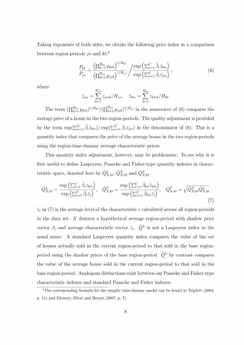
Taking exponents of both sides, we obtain the following price index in a comparison

between region-periods js and kt:5

Pkt

Pjs

=

(∏Hkth=1 pkth

)1/Hkt

(∏Hjs

h=1 pjsh

)1/Hjs

/exp

(∑Cc=1 βczktc

)exp

(∑Cc=1 βczjsc

) , (6)

where

zjsc =Hjs∑h=1

zjsch/Hjs, zktc =Hkt∑h=1

zktch/Hkt.

The term (∏Hkt

h=1 pkth)1/Hkt/(

∏Hjs

h=1 pjsh)1/Hjs in the numerator of (6) compares the

average price of a house in the two region-periods. The quality adjustment is provided

by the term exp(∑C

c=1 βczktc)/ exp(∑C

c=1 βczjsc) in the denominator of (6). This is a

quantity index that compares the price of the average house in the two region-periods

using the region-time-dummy average characteristic prices.

This quantity index adjustment, however, may be problematic. To see why it is

first useful to define Laspeyres, Paasche and Fisher-type quantity indexes in charac-

teristic space, denoted here by QLX,kt, QP

X,kt and QFX,kt.

QLX,kt =

exp(∑C

c=1 βczktc

)exp

(∑Cc=1 βczc

) , QPX,kt =

exp(∑C

c=1 βktczktc

)exp

(∑Cc=1 βktczc

) , QFX,kt =

√QP

X,ktQLX,kt

(7)

zc in (7) is the average level of the characteristic c calculated across all region-periods

in the data set. X denotes a hypothetical average region-period with shadow price

vector βc and average characteristic vector zc. QL is not a Laspeyres index in the

usual sense. A standard Laspeyres quantity index compares the value of the set

of houses actually sold in the current region-period to that sold in the base region-

period using the shadow prices of the base region-period. QL by contrast compares

the value of the average house sold in the current region-period to that sold in the

base region-period. Analogous distinctions exist between our Paasche and Fisher-type

characteristic indexes and standard Paasche and Fisher indexes.

5The corresponding formula for the simpler time-dummy model can be found in Triplett (2004;

p. 51) and Diewert, Silver and Heravi (2007; p. 7).

8

The denominator in (6) can now be rewritten as follows:

exp(∑C

c=1 βczktc

)exp

(∑Cc=1 βczjsc

) =

exp(∑C

c=1 βczktc

)exp

(∑Cc=1 βczc

)/exp

(∑Cc=1 βczjsc

)exp

(∑Cc=1 βczc

) =

QLX,kt

QLX,js

. (8)

Substituting (8) into (6), we obtain that

Pkt

Pjs

=

(∏Hkth=1 pkth

)1/Hkt

(∏Hjs

h=1 pjsh

)1/Hjs

/QL

X,kt

QLX,js

. (9)

The problem with the region-time-dummy method arises because a Laspeyres index

is subject to substitution bias. This would not itself matter if the bias was the same

for all region-periods. This, however, is unlikely to be the case. The more different a

region-period is from the average region-period denoted here by X the larger will be

the substitution bias. In the empirical part of this paper we show that in a housing

context Laspeyres has an upward bias. Suppose the bias is bigger for QLX,kt than for

QLX,js. It follows that the ratio QL

X,kt/QLX,js will be too large and hence Pkt/Pjs too

small.

A good indicator of the size of the substitution bias is provided by the ratio of a

Laspeyres-type index to a Fisher-type index:

Biaskt =QL

X,kt

QFX,kt

− 1. (10)

For example, a value of 0.1 implies a 10 percent bias. A negative value implies that

the bias acts in the opposite direction.

The region-time-dummy results will be distorted by substitution bias if the bias

differs significantly across region-periods. Of even greater concern is the possibility

that the bias may have a systematic pattern. In the empirical section we find that

this is indeed the case. The bias is systematically larger in richer regions in any given

year. It follows that the region-time-dummy method has a tendency to underestimate

differences in price levels across regions.

This is not a surprising result once it is realized that the region-time-dummy

method is an example of an average price method [see for example Hill (1997)]. In

9

the multilateral price index literature it is well known that average price methods

such as the Geary-Khamis method that underlies the Penn World Table are subject

to substitution bias [see for example Dowrick and Quiggin (1997), Hill (2000) and

Neary (2004)].

We return to these issues again in the empirical section. For the time being it

suffices to note that substitution bias creates systematic distortions in the region-

time-dummy results. Similar criticisms apply to the time-dummy method which

has enjoyed widespread use in the hedonic literature both in a housing context [see

Gourieroux and Laferrere (2006) and Diewert (2007)] and in other markets [see

Berndt, Griliches and Rappaport (1995) and Silver and Heravi (2001)]. de Haan

(2004), Silver and Heravi (2007) and Diewert, Heravi and Silver (2007) have ex-

amined the algebraic difference between time-dummy and hedonic imputation price

indexes (in the case of a single quality characteristic) and find that it is related to

the product of the difference in parameters and the change in average characteristics.

They do not, however, connect this difference to substitution bias, and hence do not

come down clearly in favor of the hedonic imputation method.

This problem of substitution bias provides the main rationale for considering

other methods such as the hedonic imputation method discussed below. The hedonic

imputation method, however, is not suitable as it stands for making multilateral

comparisons. We show later how it can be extended for this purpose. We begin

though by outlining the standard (i.e., bilateral) version of this method.

2.2 Hedonic Imputation Methods

Hedonic imputation methods impute prices for products that are missing in a par-

ticular region-period thus allowing standard price index formulas to be used. The

imputation approach is recommended by Griliches (1990; p. 189), and has been used

by the US Census Bureau to construct its housing price index. More recently, Pakes

(2003) has used it, although not in a housing context.

10

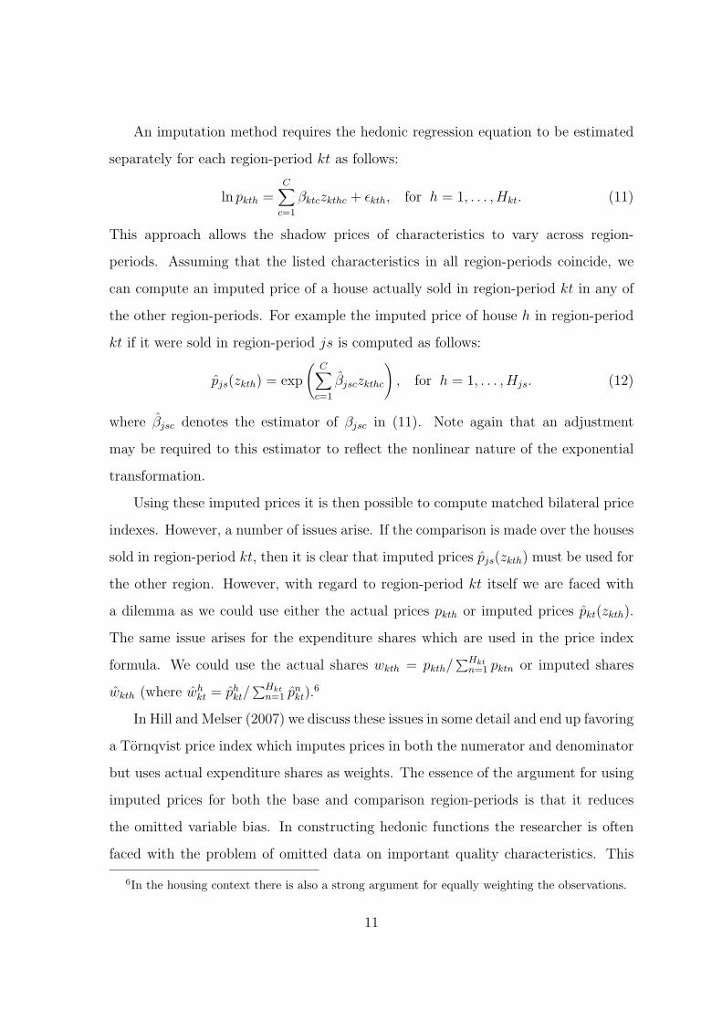
An imputation method requires the hedonic regression equation to be estimated

separately for each region-period kt as follows:

ln pkth =C∑

c=1

βktczkthc + εkth, for h = 1, . . . , Hkt. (11)

This approach allows the shadow prices of characteristics to vary across region-

periods. Assuming that the listed characteristics in all region-periods coincide, we

can compute an imputed price of a house actually sold in region-period kt in any of

the other region-periods. For example the imputed price of house h in region-period

kt if it were sold in region-period js is computed as follows:

pjs(zkth) = exp

(C∑

c=1

βjsczkthc

), for h = 1, . . . , Hjs. (12)

where βjsc denotes the estimator of βjsc in (11). Note again that an adjustment

may be required to this estimator to reflect the nonlinear nature of the exponential

transformation.

Using these imputed prices it is then possible to compute matched bilateral price

indexes. However, a number of issues arise. If the comparison is made over the houses

sold in region-period kt, then it is clear that imputed prices pjs(zkth) must be used for

the other region. However, with regard to region-period kt itself we are faced with

a dilemma as we could use either the actual prices pkth or imputed prices pkt(zkth).

The same issue arises for the expenditure shares which are used in the price index

formula. We could use the actual shares wkth = pkth/∑Hkt

n=1 pktn or imputed shares

wkth (where whkt = ph

kt/∑Hkt

n=1 pnkt).

6

In Hill and Melser (2007) we discuss these issues in some detail and end up favoring

a Tornqvist price index which imputes prices in both the numerator and denominator

but uses actual expenditure shares as weights. The essence of the argument for using

imputed prices for both the base and comparison region-periods is that it reduces

the omitted variable bias. In constructing hedonic functions the researcher is often

faced with the problem of omitted data on important quality characteristics. This

6In the housing context there is also a strong argument for equally weighting the observations.

11

is especially true for housing. In general this will bias the coefficient estimates and

as a consequence our price indexes. This bias is minimized by comparing the two

estimated hedonic functions, which will both reflect the omitted variable problem,

rather than an estimated price with an actual price. As long as the true hedonic

function of the two region-periods are not too different then it is likely that the bias

in the estimators will at least partially offset each other.

Our preferred Tornqvist index is multiplicative and, when used in conjunction

with the logarithmic hedonic model, has the desirable property that it can be decom-

posed into the multiplicative effects of individual prices and characteristics. This can

be useful in interpreting the results. The Tornqvist double imputation price index is

defined below.

Geometric Paasche : PGPjs,kt =

Hkt∏h=1

[pkt(zkth)

pjs(zkth)

]1/Hkt

, (13)

Geometric Laspeyres : PGLjs,kt =

Hjs∏h=1

[pkt(zjsh)

pjs(zjsh)

]1/Hjs , (14)

Tornqvist : P Tjs,kt =

√PGP

js,kt × PGLjs,kt, (15)

To see the desirable properties of this index consider the following decomposition

of the Geometric Paasche index.

PGPjs,kt =

Hkt∏h=1

[pkt(zkth)

pjs(zkth)

]1/Hkt

=

Hkt∏h=1

exp

[C∑

c=1

(βktc − βjsc)zkthc

]1/Hkt

= exp

1

Hkt

Hkt∑h=1

C∑c=1

(βktc − βjsc)zkthc

= exp

C∑c=1

(βktc − βjsc)Hkt∑h=1

zkthc/Hkt

= exp

[C∑

c=1

(βktc − βjsc)zktc

],

where zktc =∑Hkt

h=1 zkthc/Hkt. Combining this with an analogous decomposition for

12

Geometric Laspeyres, it follows that Tornqvist can be written as follows:

P Tjs,kt = exp

[1

2

C∑c=1

(βktc − βjsc)(zjsc + zktc)

]

= exp

[C∑

c=1

(βktc − βjsc)zjs−kt,c

], (16)

where zjs−kt,c = (zjsc + zktc)/2. That is, it can be decomposed into multiplicative con-

tributions from each of the characteristics. For our purposes, an even more pertinent

decomposition is the following:

P Tjs,kt =

Hkt∏h=1

[pkt(zkth)

pjs(zkth)

]1/Hkt

×Hjs∏h=1

[pkt(zjsh)

pjs(zjsh)

]1/Hjs

1/2

=

[∏Hkth=1 pkt(zkth)

]1/Hkt

[∏Hjs

h=1 pjs(zjsh)]1/Hjs

/exp

[C∑

c=1

(βjsc + βktc)

2(zktc − zjsc)

]

=

[∏Hkth=1 pkt(zkth)

]1/Hkt

[∏Hjs

h=1 pjs(zjsh)]1/Hjs

/QT

kt,js . (17)

We now have a firm basis for comparing the region-time-dummy method and the

hedonic imputation method. A striking similarity exists between equations (9) and

(17). The key difference is that the quantity indexes in the denominator of (9) are of

the Laspeyres type and are calculated using the shadow prices of the average region-

period X. Hence they are affected by substitution bias.7 By contrast, the quantity

index in the denominator of (17) is Tornqvist which is calculated using the shadow

prices of only region-periods js and kt. The Tornqvist index’s symmetric treatment

of both region-periods ensures that it is free of substitution bias.

Empirical support for these claims is provided later in the paper. The fact that

the imputation approach is free of substitution bias is a significant advantage and

leads us to prefer it over the region-time-dummy approach.

7The one exception is when this method is implemented in a bilateral setting. In a temporal

context, Triplett (2004) refers to this as the adjacent period method. In this case, the average price

vector βc should be equally representative of both region-periods.

13

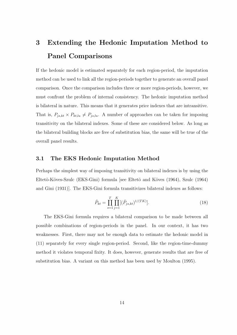
3 Extending the Hedonic Imputation Method to

Panel Comparisons

If the hedonic model is estimated separately for each region-period, the imputation

method can be used to link all the region-periods together to generate an overall panel

comparison. Once the comparison includes three or more region-periods, however, we

must confront the problem of internal consistency. The hedonic imputation method

is bilateral in nature. This means that it generates price indexes that are intransitive.

That is, Pjs,kt × Pkt,lu 6= Pjs,lu. A number of approaches can be taken for imposing

transitivity on the bilateral indexes. Some of these are considered below. As long as

the bilateral building blocks are free of substitution bias, the same will be true of the

overall panel results.

3.1 The EKS Hedonic Imputation Method

Perhaps the simplest way of imposing transitivity on bilateral indexes is by using the

Elteto-Koves-Szulc (EKS-Gini) formula [see Elteto and Koves (1964), Szulc (1964)

and Gini (1931)]. The EKS-Gini formula transitivizes bilateral indexes as follows:

Pkt =T∏

s=1

K∏j=1

[(Pjs,kt)1/(TK)]. (18)

The EKS-Gini formula requires a bilateral comparison to be made between all

possible combinations of region-periods in the panel. In our context, it has two

weaknesses. First, there may not be enough data to estimate the hedonic model in

(11) separately for every single region-period. Second, like the region-time-dummy

method it violates temporal fixity. It does, however, generate results that are free of

substitution bias. A variant on this method has been used by Moulton (1995).

14

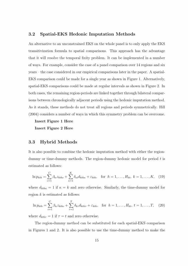
3.2 Spatial-EKS Hedonic Imputation Methods

An alternative to an unconstrained EKS on the whole panel is to only apply the EKS

transitivization formula to spatial comparisons. This approach has the advantage

that it will resolve the temporal fixity problem. It can be implemented in a number

of ways. For example, consider the case of a panel comparison over 14 regions and six

years – the case considered in our empirical comparisons later in the paper. A spatial-

EKS comparison could be made for a single year as shown in Figure 1. Alternatively,

spatial-EKS comparisons could be made at regular intervals as shown in Figure 2. In

both cases, the remaining region-periods are linked together through bilateral compar-

isons between chronologically adjacent periods using the hedonic imputation method.

As it stands, these methods do not treat all regions and periods symmetrically. Hill

(2004) considers a number of ways in which this symmetry problem can be overcome.

Insert Figure 1 Here

Insert Figure 2 Here

3.3 Hybrid Methods

It is also possible to combine the hedonic imputation method with either the region-

dummy or time-dummy methods. The region-dummy hedonic model for period t is

estimated as follows:

ln pkth =C∑

c=1

βtczkthc +K∑

κ=1

δκtdkthκ + εkth, for h = 1, . . . , Hkt, k = 1, . . . , K, (19)

where dkthκ = 1 if κ = k and zero otherwise. Similarly, the time-dummy model for

region k is estimated as follows:

ln pkth =C∑

c=1

βtczkthc +T∑

τ=1

δkτdkthτ + εkth, for h = 1, . . . , Hkt, t = 1, . . . , T, (20)

where dkthτ = 1 if τ = t and zero otherwise.

The region-dummy method can be substituted for each spatial-EKS comparison

in Figures 1 and 2. It is also possible to use the time-dummy method to make the

15

temporal comparisons instead of the hedonic imputation method. The problem with

such hybrid methods is that they introduce substitution bias into the results through

the use of either the region-dummy or time-dummy methods. Use of the time-dummy

method will also lead to violations of temporal fixity.

4 The Results and Their Interpretation

4.1 The Data Set

Most of our data set was obtained from Australian Property Monitors and consists

of prices and characteristics of houses sold in 198 postcodes in Sydney for the years

2001-2006. Out of a total of 750,000 observations (i.e. house sales), information on

characteristics were available for 173,329 or 21.4 percent of our sample. Our hedonic

analysis was restricted to these 173,329 observations.8 The characteristics we have

for each property are sale price, time of sale (quarter/year), postcode, dwelling type

(i.e., house or apartment), number of bedrooms, number of bathrooms, and land area

(for houses only).

4.2 Temporal and Spatial Index Results

Results for 14 regions in Sydney over six years are provided for two panel methods.

The 14 regions are as follows: 1=Inner Sydney, 2=Eastern Suburbs, 3=Inner West,

4=Lower North Shore, 5=Upper North Shore, 6=Mosman and Cremorne, 7=Manly

Warringah, 8=North Western, 9=Western Suburbs, 10=Parramatta Hills, 11=Fair-

field Liverpool, 12=Canterbury Bankstown, 13=St George, 14=Cronulla Sutherland.

The first panel method considered is the region-time-dummy method defined in

(3). In practice, we make a minor modification to the standard region-time-dummy

method to control for sub-regional and sub-annual price change. Instead of insert-

8This could introduce sample selection bias into the results. This is not a major concern for us

since our focus is on methodological issues. The results are meant only to be illustrative.

16

ing dummy variables for each region-year we specify dummies for each postcode (a

sub-regional grouping) within a region-year, and for each quarter within a region-

year. This allows us to more specifically control for compositional change. The use of

postcode dummy variables accounts for any sub-regional differences in amenities, and

hence means that changes in the number of sales across cheaper or more expensive

postcodes within a region will not distort the results. In order to estimate the price

level for a region-period we evaluate the postcode and quarterly dummy variables

at the sample mean (i.e. a particular region-period price level is a weighted aver-

age of postcode and quarter dummy variables where the weights are the number of

transactions in each cell over the entire sample). This modification of the time-region-

dummy method makes us confident that our results reflect pure price differences and

not compositional changes in the houses being sold in a given region-period. The

model is estimated using OLS.9 The estimated region-time-dummy price indexes for

each region-period are shown in Table 1.

Insert Table 1 Here

The second panel method considered is the EKS method as defined in (18). This

requires the hedonic model to be estimated separately for each region-period. The

hedonic imputation method is then used to compare all possible pairs of region-

periods, and the resulting indexes are transitivized using the EKS formula. The

resulting price indexes are shown in Table 2.

Insert Table 2 Here

A comparison between the results in Tables 1 and 2 is particularly revealing.

These results are combined in Table 3 with the price index for each region-period for

both methods normalized to 1 in 2001. That is, the focus in Table 3 is on temporal

price changes. This normalization allows us to compare the growth rates of prices over

9Longitude and latitude are often used to construct a spatial correlation matrix to correct for

spatial omitted variables [see for example Anselin (1988) and Pace, Barry and Sirmans (1998)]. We

do not do this here. The use of double imputation in the hedonic imputation method already at

least partially corrects for omitted variables.

17

time across each region. It is striking that for 13 of the 14 regions, prices rose less from

2001 to 2006 according to the region-time-dummy method. Differences in the spatial

dimension are compared in Table 4. The standard deviation of the log price indexes

generated by the region-time-dummy and EKS methods for each year are shown in

the first two rows. These standard deviations measure the dispersion in average prices

across the 14 regions. A higher standard deviation implies greater dispersion. For all

six years, the standard deviation is smaller for the region-time-dummy method.

Insert Table 3 Here

Insert Table 4 Here

4.3 Evidence of Substitution Bias

The systematic differences between the region-time-dummy and EKS results described

in Tables 3 and 4 can be attributed to substitution bias in the region-time-dummy

results. The bias has two contributory causes. First, the Laspeyres-type quantity

indexes in characteristics space QLX,kt defined in (7) tend to be systematically larger

than their Paasche counterparts QPX,kt. This result is observed for 63 of the 84 region-

periods. This finding is consistent with the following substitution effect for each

characteristic c:pktc

pjsc

− P Fjs,kt > 0⇔ zktc

zjsc

− QFjs,kt < 0, (21)

where pktc and qktc denote the average price and quantity of characteristic c in region-

period kt. The interpretation of this relationship is best illustrated with an exam-

ple. Suppose there are only two characteristics: bedrooms and bathrooms. Sup-

pose further that on average houses sold in region-period js have two bedrooms

and two bathrooms, while houses sold in kt have three bedrooms and two bath-

rooms. It follows from the fact that kt has more of one characteristic and the

same of the other that QFjs,kt > 1. Also, if we focus on the bathroom character-

istic, we know that qkt,bath/qjs,bath = 1. Plugging these results into (21) we obtain

that pkt,bath/pjs,bath > P Fjs,kt. That is, the bathroom shadow price ratio should ex-

18

ceed the price difference between houses in the two region-periods. This result seems

intuitively reasonably plausible.

The second contributory factor is that the substitution bias is systematically

larger in the richer regions. To show that this is the case, we compute correlation

coefficients between substitution bias as defined in (10) and price level as measured

by EKS and depicted in Table 2 across all regions for each year. The correlation

coefficients are as follows: 2001=0.2685, 2002=0.5256, 2003=0.5568, 2004=0.4730,

2005=0.4900, 2006=0.5981. In all cases the correlation coefficient is positive. That

is, a positive correlation exists between price level and substitution bias in each year.

This suggests that the richest regions are outliers in terms of their price and quantity

characteristics vectors. This finding combined with the fact that Laspeyres usually

exceeds Paasche explains the finding in Table 4 that the region-time-dummy method

tends to systematically underestimate differences in price levels across regions. In

addition, the regions for which Paasche exceeds Laspeyres tend to be the low priced

ones. It is possible that the substitution effect may actually reverse direction in some

low price regions. In particular, according to EKS, region 12 is the second cheapest in

all six years. At the same time, every year Paasche exceeds Laspeyres for region 12.

Irrespective of its cause, the concentration of cases where Paasche exceeds Laspeyres

in the poorest regions further exacerbates the substitution bias in the region-time-

dummy results.

Perhaps the most conclusive demonstration of substitution bias in the region-

time-dummy results is provided by the Laspeyres and Paasche Limited Characteristic

results in Table 4 denoted here by LLC and PLC respectively. The LLC results are

computed using the following formula:

Pkt

Pjs

=

(∏Hkth=1 pkth

)1/Hkt

(∏Hjs

h=1 pjsh

)1/Hjs

/QL

X,kt

QLX,js

,

whereQL

X,kt

QLX,js

=

exp(∑C

c=1 βczktc

)exp

(∑Cc=1 βczc

)/exp

(∑Cc=1 βczjsc

)exp

(∑Cc=1 βczc

) . (22)

19

This formula is the same as the one used by the region-time-dummy method in (6)

with one important difference. This is that the Laspeyres quantity indexes are only

calculated over the four characteristics common to all region-periods, namely dwelling

type, number of bedrooms, number of bathrooms and land area. That is, no account

is taken of the postcode and quarter dummy variables. Similarly, the PLC results are

computed as follows:

Pkt

Pjs

=

(∏Hkth=1 pkth

)1/Hkt

(∏Hjs

h=1 pjsh

)1/Hjs

/QP

X,kt

QPX,js

,

whereQP

X,kt

QPX,js

=

exp(∑C

c=1 βktczktc

)exp

(∑Cc=1 βktczc

)/exp

(∑Cc=1 βjsczjsc

)exp

(∑Cc=1 βjsczc

) . (23)

The PLC method differs from the LLC method in that it uses the hedonic imputa-

tion shadow prices (βktc) from (11) instead of the region-time-dummy shadow prices.

Again the comparison is restricted to dwelling type, number of bedrooms, number of

bathrooms and land area. These shadow prices are shown in Table 5.10

Insert Table 5 Here

Standard deviations of log prices indexes generated by the LLC and PLC methods

for each year are shown in Table 4. The results are striking in two respects. First, the

price level dispersion for the LLC method is almost the same as that of the region-

time-dummy method. These results differ on average by about one percent, and the

differences do not seem to be systematic in any way. In other words, the LLC method

provides a good approximation to the region-time-dummy method. Second, from a

comparison of the LLC and PLC results it can be seen that for each year the price

level dispersion is higher for PLC than for LLC. Furthermore, for all six years, the

EKS results lie in between the PLC and LLC results. The PLC and LLC results,

therefore, demonstrate how much substitution bias can distort the results while at

10We observe a very small number of negative shadow prices. They have a negligible impact on

the results. Hence it is not necessary to impose a nonnegativity constraint on the shadow prices

when estimating the hedonic models in (3) and (11).

20

the same time providing further evidence that the EKS results are free of substitution

bias.

Similarly the finding in Table 3 that the region-time-dummy prices rise system-

atically too slowly can also be explained in terms of substitution bias. The av-

erage substitution biases for each year are as follows: 2001=0.0148, 2002=0.0156,

2003=0.0224, 2004=0.0193, 2005=0.0172, 2006=0.0182. It follows that 2003 and

2004 are the biggest outliers in terms of price and quantity characteristics vectors in

the sample. This makes sense given that house prices for Sydney as a whole followed

an inverted U-curve over this period peaking in 2003/4. Closer inspection of Table 3

reveals that for 13 of the 14 regions, the gap between the EKS and region-time-dummy

price indexes (with prices normalized to 1 in 2001) in 2004 was greater than in 2006.

That is, the region-time-dummy prices rise faster than EKS prices from 2001 to 2004

for all 14 regions. From 2004 to 2006 this pattern reverses for all regions except one.

In other words, while the average substitution bias is rising from one year to the

next, the region-time-dummy results will tend to rise too slowly. When the average

substitution bias starts to fall this pattern reverses.

4.4 Movements in Mean and Median House Prices

Finally, we consider how simple mean and median price indexes compare with our

hedonic indexes. The changes in the geometric mean and median price indexes for

each of the 14 regions are shown in Table 6. The geometric mean index rises less than

the EKS index (see Table 2) in the nine richest regions, and rises more in the other

five regions. For the median the pattern is similar. The median price index rises

less than EKS in 11 regions, the exceptions being three of the five poorest regions.

In other words, simple average measures systematically underestimate house price

inflation over the 2001-2006 period except for the poorest regions for which they tend

to overestimate inflation. This finding implies that the average quality of the houses

sold has improved over the 2001-2006 except for the poorest regions where it has

21

worsened.

Insert Table 6 Here

It can be seen from the last two rows of Table 4 that the geometric mean and

median measures systematically underestimate differences in price levels across re-

gions each year. This can again be attributed to their failure to account for quality

differences. The houses sold in richer areas on average tend to be of higher quality.

Simple average measures ignore this fact.

5 Conclusion

In this paper we have developed a methodology for constructing hedonic price in-

dexes on panel data sets from bilateral building blocks constructed using the hedonic

imputation method. We have also shown that the widely used time-dummy and

region-dummy hedonic methods are prone to substitution bias. The same is true

of the region-time-dummy method which extends these methods to a panel context.

It is mainly for this reason that we favor panel methods constructed from bilateral

building blocks. By applying our methodology to housing data for Sydney for 14

regions covering a six year period, we have been able to show that in this case at least

the substitution bias in the region-time-dummy results is quite pronounced. Simple

average measures of house prices exhibit even more bias than the region-time-dummy

method. This is because of their failure to account for quality differences in the hous-

ing sold in richer and poorer regions, and the fact that in all but the poorest regions

average quality is improving over time.

6 References

Aizcorbe, A. and B. Aten (2004), “An Approach to Pooled Time and Space Com-

parisons,” Paper presented at the SSHRC Conference on Index Number Theory

and the Measurement of Prices and Productivity, Vancouver, Canada.

22

Anselin, L. (1988), Spatial Econometrics: Methods and Models. Dordrecht: Kluwer.

Baily, M. J., R. F. Muth and H. O. Nourse (1963), “A Regression Method for Real

Estate Price Index Construction,” Journal of the American Statistical Association

58, 933-942.

Bao, H. X. H. and A. T. K. Wan (2004), “On the Use of Spline Smoothing in

Estimating Hedonic Housing Price Models: Empirical Evidence Using Hong Kong

Data,” Real Estate Economics 32(3), 487-507.

Berndt, E. R., Z. Griliches and N. J. Rappaport (1995), “Econometric Estimates of

Price Indexes for Personal Computers in the 1990’s,” Journal of Econometrics

68(1), 243-268.

Court, A. T. (1939), “Hedonic Price Indexes with Automotive Examples,” in The

Dynamics of Automobile Demand. The General Motors Corporation, New York,

99-117.

Cutler, D. M. and E. R. Berndt, eds. (2001), Medical Care Output and Productivity,

NBER Studies in Income and Wealth, vol. 62. Chicago and London: University

of Chicago Press.

Demographia (2008), 4th Annual Demographia International Housing Affordability

Survey, �www.demographia.com�.

Diewert, W. E. (2003), “Hedonic Regressions: A Review of Some Unresolved Issues,”

Mimeo.

Diewert, W. E. (2007), “The Paris OECD-IMF Workshop on Real Estate Price In-

dexes: Conclusions and Future Directions,” Discussion Paper 07-01, Department

of Economics, University of British Columbia.

Diewert, W. E., S. Heravi and M. Silver (2007), “Hedonic Imputation Indexes versus

Time Dummy Hedonic Indexes,” IMF Working Paper, WP/07/234.

Dowrick, S. and J. Quiggin (1997), “True Measures of GDP and Convergence,”

American Economic Review 87(1), 41-64.

23

Dreiman, M. H. and A. Pennington-Cross (2004), “Alternative Methods of Increasing

the Precision of Weighted Repeated Sales House Price Indices,” Journal of Real

Estate Finance and Economics 28(4), 299-317.

Dulberger, E. R. (1989), “The Application of a Hedonic Model to a Quality-Adjusted

Price Index for Computer Processors,” in D. W. Jorgenson and R. Landau (eds.),

Technology and Capital Formation, Cambridge, MA: MIT Press, 37-75.

Elteto, O. and P. Koves (1964), “On a Problem of Index Number Computation

Relating to International Comparison.” Statisztikai Szemle 42, 507-518.

Englund, P., J. M. Quigley and C. L. Redfearn (1998), “Improved Price Indexes for

Real Estate: Measuring the Course of Swedish Housing Prices,” Journal of Urban

Economics 44, 171-196.

Garderen, K. J. van and C. Shah (2002), “Exact Interpretation of Dummy Variables

in Semilogarithmic Equations” Econometrics Journal 5, 149-159.

Garino, G. and L. Sarno (2004), “Speculative Bubbles in U.K. House Prices: Some

New Evidence,” Southern Economic Journal 70(4), 777-795.

Giles, D. E. A. (1982), “The Interpretation of Dummy Variables in Semilogarithmic

Equations,” Economics Letters 10, 77-79.

Gini, C. (1931), “On the Circular Test of Index Numbers.” International Review of

Statistics, 9(2), 3-25.

Glaeser E. and J. Gyourko (2003), “The Impact of Zoning on Housing Affordability,”

Economic Policy Review 9(2), 21-39.

Goodhart, C. (2001), “What Weight Should Be Given to Asset Prices in the Mea-

surement of Inflation?” Economic Journal 111(472), F335-356.

Gourieroux, C. and A. Laferrere (2006), “Managing Hedonic Housing Price Indexes:

The French Experience,” Paper presented at the OECD-IMF Workshop on Real

Estate Price Indexes, Paris, November 6-7.

24

Griliches, Z. (1961), “Hedonic Price Indexes for Automobiles: An Econometric Anal-

ysis of Quality Change,” in The Price Statistics of the Federal Government, G.

Stigler (chairman). Washington D.C.: Government Printing Office.

Griliches, Z. (1990), “Hedonic Price Indexes and the Measurement of Capital and

Productivity,” in Fifty Years of Economic Measurement, E. R. Berndt and J. E.

Triplett (eds.). Chicago: Chicago University Press and NBER, 185-202.

Hill, R. J. (1997), “A Taxonomy of Multilateral Methods for Making International

Comparisons of Prices and Quantities,” Review of Income and Wealth 43(1),

49-69.

Hill, R. J. (2000), “Measuring Substitution Bias in International Comparisons Based

on Additive Purchasing Power Parity Methods,” European Economic Review

44(1), 145-162.

Hill, R. J. (2004), “Constructing Price Indexes Across Countries and Time: The

Case of the European Union,” American Economic Review 94(5), 1379-1410.

Hill, R. J. and D. Melser (2007), “Hedonic Imputation and the Price Index Problem:

An Application to Housing,” Economic Inquiry, forthcoming.

Hoffman, J. and A. Lorenz (2006), “Real Estate Price Indices for Germany: Past,

Present and Future,” Paper presented at the OECD-IMF Workshop on Real

Estate Price Indexes, Paris, November 6-7.

Ito, T. and T. Iwaisako (1996), “Explaining Asset Bubbles in Japan,” Monetary and

Economic Studies 14(1), 143-193.

Kennedy, P. E. (1981), Estimation with Correctly Interpreted Dummy Variables in

Semilogarithmic Equations,” American Economic Review 71 (4), 801.

Martins-Filho, C. and O. Bin (2005), “Estimation of Hedonic Price Functions via

Additive Nonparametric Regression,” Empirical Economics 30(1), 93-114.

Moulton, B. R. (1995), “Interarea Indexes of the Cost of Shelter using Hedonic

Quality Adjustment Techniques,” Journal of Econometrics 68(1), 181-204.

25

Neary, J. P. (2004), “Rationalizing the Penn World Table: True Multilateral In-

dices for International Comparisons of Real Income,” American Economic Review

94(5), 1411-1428.

Pace, R. K. (1993), “Nonparametric Methods with Application to Hedonic Models,”

Journal of Real Estate Finance and Economics 7(3), 185-204.

Pace, R. K., R. Barry and C. F. Sirmans (1998), “Spatial Statistics and Real Estate,”

Journal of Real Estate Finance and Economics 17(1), 5-13.

Pakes, A. (2003), “A Reconsideration of Hedonic Price Indexes with an Application

to PC’s,” American Economic Review 93(5), 1578-1596.

Rosen, S. (1974), “Hedonic Prices and Implicit Markets: Product Differentiation in

Pure Competition,” Journal of Political Economy 82(1), 34-55.

Shiller, R. J. (1991), “Arithmetic Repeat Sales Price Estimators,” Journal of Housing

Economics 1, 110-126.

Shiller, R. J. (1993), “Measuring Asset Values for Cash Settlement in Derivative

Markets: Hedonic Repeated Measures Indices and Perpetual Futures,” Journal

of Finance 48(3), 911-931.

Silver, M. and S. Heravi (2001), “Scanner data and the Measurement of Inflation,”

Economic Journal 111(472), F383-F404.

Silver, M. and S. Heravi (2007), “The Difference Between Hedonic Imputation In-

dexes and Time Dummy Hedonic Indexes,” Journal of Business and Economic

Statistics 25(2), 239-246.

Szulc, B. J. (1964), “Indices for Multiregional Comparisons,” Przeglad Statystyczny

3, Statistical Review 3, 239-254.

Triplett, J. E. (1969), “Automobiles and Hedonic Quality Measurement,” Journal of

Political Economy 77(3), 408-417.

Triplett, J. E. (1990), “Hedonic Methods in Statistical Agency Environments: An

26

Intellectual Biopsy,” in Fifty Years of Economic Measurement, E. R. Berndt and

J. E. Triplett (eds.). Chicago: Chicago University Press and NBER, 207-233.

Triplett, J. E. (2004), Handbook on Hedonic Indexes and Quality Adjustments in

Price Indexes: Special Application to Information Technology Products, STI Work-

ing Paper 2004/9, Directorate for Science, Technology and Industry, Organisation

for Economic Co-operation and Development, Paris.

27

FIGURE 1. — HEDONIC IMPUTATION: SPATIAL-EKS (SINGLE SPATIAL

BENCHMARK CASE) COMBINED WITH TEMPORAL CHRONOLOGICAL

CHAINING

2001

2002

2003

2004

2005

2006

2001

2002

2003

2004

2005

2006

1 2 3 4 5 6 7 8 9 10 11 12 13 14

1 2 3 4 5 6 7 8 9 10 11 12 13 14

�� � s s s s s s s s s s s s s ss s s s s s s s s s s s s ss s s s s s s s s s s s s ss s s s s s s s s s s s s ss s s s s s s s s s s s s ss s s s s s s s s s s s s s

FIGURE 2. — HEDONIC IMPUTATION: SPATIAL-EKS AT 4 PERIOD

INTERVALS COMBINED WITH TEMPORAL CHRONOLOGICAL CHAINING

THROUGH REGION C

2001

2002

2003

2004

2005

2006

2001

2002

2003

2004

2005

2006

1 2 3 4 5 6 7 8 9 10 11 12 13 14

1 2 3 4 5 6 7 8 9 10 11 12 13 14

�� �

�� �

s s s s s s s s s s s s s ss s s s s s s s s s s s s ss s s s s s s s s s s s s ss s s s s s s s s s s s s ss s s s s s s s s s s s s ss s s s s s s s s s s s s s

28

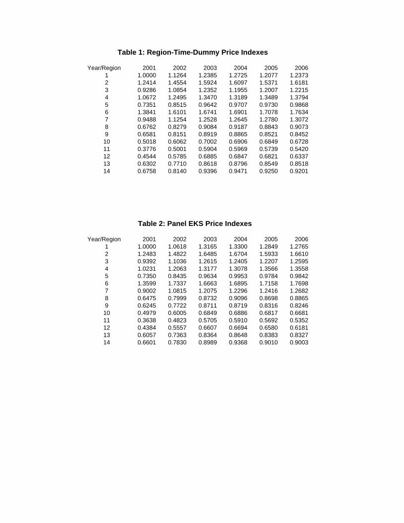
Table 1: Region-Time-Dummy Price Indexes

Year/Region 2001 2002 2003 2004 2005 20061 1.0000 1.1264 1.2385 1.2725 1.2077 1.23732 1.2414 1.4554 1.5924 1.6097 1.5371 1.61813 0.9286 1.0854 1.2352 1.1955 1.2007 1.22154 1.0672 1.2495 1.3470 1.3189 1.3489 1.37945 0.7351 0.8515 0.9642 0.9707 0.9730 0.98686 1.3841 1.6101 1.6741 1.6901 1.7078 1.76347 0.9488 1.1254 1.2528 1.2645 1.2780 1.30728 0.6762 0.8279 0.9084 0.9187 0.8843 0.90739 0.6581 0.8151 0.8919 0.8865 0.8521 0.845210 0.5018 0.6062 0.7002 0.6906 0.6849 0.672811 0.3776 0.5001 0.5904 0.5969 0.5739 0.542012 0.4544 0.5785 0.6885 0.6847 0.6821 0.633713 0.6302 0.7710 0.8618 0.8796 0.8549 0.851814 0.6758 0.8140 0.9396 0.9471 0.9250 0.9201

Table 2: Panel EKS Price Indexes

Year/Region 2001 2002 2003 2004 2005 20061 1.0000 1.0618 1.3165 1.3300 1.2849 1.27652 1.2483 1.4822 1.6485 1.6704 1.5933 1.66103 0.9392 1.1036 1.2615 1.2405 1.2207 1.25954 1.0231 1.2063 1.3177 1.3078 1.3566 1.35585 0.7350 0.8435 0.9634 0.9953 0.9784 0.98426 1.3599 1.7337 1.6663 1.6895 1.7158 1.76987 0.9002 1.0815 1.2075 1.2296 1.2416 1.26828 0.6475 0.7999 0.8732 0.9096 0.8698 0.88659 0.6245 0.7722 0.8711 0.8719 0.8316 0.824610 0.4979 0.6005 0.6849 0.6886 0.6817 0.668111 0.3638 0.4823 0.5705 0.5910 0.5692 0.535212 0.4384 0.5557 0.6607 0.6694 0.6580 0.618113 0.6057 0.7363 0.8364 0.8648 0.8383 0.832714 0.6601 0.7830 0.8989 0.9368 0.9010 0.9003

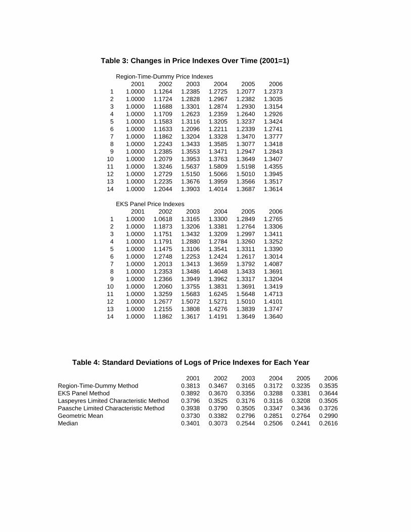
Table 3: Changes in Price Indexes Over Time (2001=1)

Region-Time-Dummy Price Indexes2001 2002 2003 2004 2005 2006

1 1.0000 1.1264 1.2385 1.2725 1.2077 1.23732 1.0000 1.1724 1.2828 1.2967 1.2382 1.30353 1.0000 1.1688 1.3301 1.2874 1.2930 1.31544 1.0000 1.1709 1.2623 1.2359 1.2640 1.29265 1.0000 1.1583 1.3116 1.3205 1.3237 1.34246 1.0000 1.1633 1.2096 1.2211 1.2339 1.27417 1.0000 1.1862 1.3204 1.3328 1.3470 1.37778 1.0000 1.2243 1.3433 1.3585 1.3077 1.34189 1.0000 1.2385 1.3553 1.3471 1.2947 1.2843

10 1.0000 1.2079 1.3953 1.3763 1.3649 1.340711 1.0000 1.3246 1.5637 1.5809 1.5198 1.435512 1.0000 1.2729 1.5150 1.5066 1.5010 1.394513 1.0000 1.2235 1.3676 1.3959 1.3566 1.351714 1.0000 1.2044 1.3903 1.4014 1.3687 1.3614

EKS Panel Price Indexes

2001 2002 2003 2004 2005 20061 1.0000 1.0618 1.3165 1.3300 1.2849 1.27652 1.0000 1.1873 1.3206 1.3381 1.2764 1.33063 1.0000 1.1751 1.3432 1.3209 1.2997 1.34114 1.0000 1.1791 1.2880 1.2784 1.3260 1.32525 1.0000 1.1475 1.3106 1.3541 1.3311 1.33906 1.0000 1.2748 1.2253 1.2424 1.2617 1.30147 1.0000 1.2013 1.3413 1.3659 1.3792 1.40878 1.0000 1.2353 1.3486 1.4048 1.3433 1.36919 1.0000 1.2366 1.3949 1.3962 1.3317 1.3204

10 1.0000 1.2060 1.3755 1.3831 1.3691 1.341911 1.0000 1.3259 1.5683 1.6245 1.5648 1.471312 1.0000 1.2677 1.5072 1.5271 1.5010 1.410113 1.0000 1.2155 1.3808 1.4276 1.3839 1.374714 1.0000 1.1862 1.3617 1.4191 1.3649 1.3640

Table 4: Standard Deviations of Logs of Price Indexes for Each Year

2001 2002 2003 2004 2005 2006Region-Time-Dummy Method 0.3813 0.3467 0.3165 0.3172 0.3235 0.3535EKS Panel Method 0.3892 0.3670 0.3356 0.3288 0.3381 0.3644Laspeyres Limited Characteristic Method 0.3796 0.3525 0.3176 0.3116 0.3208 0.3505Paasche Limited Characteristic Method 0.3938 0.3790 0.3505 0.3347 0.3436 0.3726Geometric Mean 0.3730 0.3382 0.2796 0.2851 0.2764 0.2990Median 0.3401 0.3073 0.2544 0.2506 0.2441 0.2616

Table 5: Characteristic Shadow Prices

Prices Dwelling Bedrooms Baths Land area Prices Dwelling Bedrooms Baths Land areaβRTD 0.2759 0.1451 0.1902 181.9 β8,01 0.0765 0.0967 0.2011 240.6β1,01 0.0375 0.1549 0.2839 627.5 β8,02 0.2418 0.0891 0.1765 185.6β1,02 0.2047 0.1645 0.3083 -53.3 β8,03 0.2836 0.0797 0.1773 289.0β1,03 0.0820 0.2244 0.2752 801.3 β8,04 0.2529 0.0727 0.1799 221.4β1,04 0.0854 0.2718 0.3170 475.8 β8,05 0.2915 0.1295 0.1461 135.9β1,05 0.1342 0.2196 0.2976 557.2 β8,06 0.2561 0.1288 0.1746 174.1β1,06 0.1982 0.2592 0.2996 170.2 β9,01 0.1208 0.1059 0.1264 313.3β2,01 0.1375 0.1802 0.1812 697.7 β9,02 0.1422 0.0893 0.1539 383.8β2,02 0.2044 0.1437 0.2282 791.3 β9,03 0.1570 0.1024 0.1425 522.9β2,03 0.2385 0.1824 0.1857 825.7 β9,04 0.1081 0.1199 0.1583 541.5β2,04 0.2766 0.1590 0.2239 718.4 β9,05 0.1222 0.1298 0.1434 490.3β2,05 0.2597 0.1890 0.2219 670.4 β9,06 0.1543 0.1421 0.1396 437.5β2,06 0.2418 0.2032 0.2306 721.1 β10,01 0.2033 0.0762 0.1924 -66.93β3,01 0.1310 0.1352 0.2043 537.9 β10,02 0.2355 0.0625 0.1601 -69.454β3,02 0.1410 0.1308 0.2005 711.6 β10,03 0.2647 0.0690 0.1550 -5.7041β3,03 0.1410 0.1464 0.1637 670.5 β10,04 0.3032 0.0509 0.1676 73.6β3,04 0.1868 0.1620 0.2006 588.8 β10,05 0.3103 0.1006 0.1615 -115.65β3,05 0.2234 0.1597 0.1789 446.7 β10,06 0.3662 0.0957 0.1608 -120.65β3,06 0.2021 0.1593 0.2010 542.8 β11,01 0.2026 0.1109 0.0934 122.1β4,01 0.2921 0.1501 0.2066 199.7 β11,02 0.0873 0.0783 0.1254 297.2β4,02 0.2689 0.1470 0.1595 276.2 β11,03 0.2001 0.0643 0.0910 259.8β4,03 0.2994 0.1770 0.1642 335.0 β11,04 0.2099 0.0732 0.1070 275.2β4,04 0.4482 0.1817 0.2012 135.9 β11,05 0.0935 0.1042 0.0862 303.8β4,05 0.3335 0.1947 0.1815 314.7 β11,06 0.1287 0.1201 0.1572 292.4β4,06 0.3072 0.2100 0.1486 299.5 β12,01 0.4049 -0.0492 0.1506 270.7β5,01 0.3025 0.0811 0.1688 35.1 β12,02 0.1652 0.0867 0.0985 460.9β5,02 0.3365 0.0819 0.1500 48.5 β12,03 0.2387 0.0831 0.0897 348.4β5,03 0.3174 0.0787 0.1436 63.8 β12,04 0.2897 0.0798 0.1003 257.9β5,04 0.2960 0.0885 0.1499 40.2 β12,05 0.1608 0.1055 0.0832 259.0β5,05 0.3147 0.0942 0.1631 60.6 β12,06 0.1514 0.1224 0.1390 422.7β5,06 0.3086 0.1020 0.1766 76.1 β13,01 0.0604 0.0731 0.1652 512.5β6,01 0.1185 0.2693 0.2320 454.3 β13,02 0.2210 0.0828 0.1291 365.7β6,02 0.0988 0.1953 0.0689 1190.0 β13,03 0.2502 0.0686 0.1000 517.9β6,03 0.2413 0.2811 0.1974 396.5 β13,04 0.2087 0.1154 0.1308 449.9β6,04 0.1303 0.3085 0.1696 515.7 β13,05 0.2562 0.0893 0.1264 355.4β6,05 0.0983 0.2709 0.2865 517.2 β13,06 0.2025 0.1330 0.1304 312.0β6,06 0.1857 0.2752 0.1719 626.5 β14,01 0.1200 0.0960 0.1808 257.7β7,01 0.1149 0.0931 0.2569 166.1 β14,02 0.1603 0.1305 0.1954 149.0β7,02 0.1359 0.1263 0.1686 162.5 β14,03 0.1064 0.1242 0.1607 372.6β7,03 0.2993 0.1103 0.1918 83.5 β14,04 0.2229 0.0967 0.1776 333.8β7,04 0.2523 0.1046 0.2085 225.9 β14,05 0.0810 0.1396 0.1792 358.8β7,05 0.3300 0.1223 0.2149 121.6 β14,06 0.1645 0.1139 0.2023 272.4β7,06 0.2323 0.1534 0.2164 171.0

Table 6: Changes in Average Prices Over Time (2001=1)

Geometric Mean2001 2002 2003 2004 2005 2006

1 1.0000 1.1552 1.2480 1.3156 1.2190 1.24352 1.0000 1.1400 1.2387 1.2866 1.1746 1.22363 1.0000 1.1284 1.2805 1.2981 1.2541 1.29224 1.0000 1.1183 1.2340 1.2341 1.2071 1.20565 1.0000 1.1114 1.2122 1.2858 1.1712 1.22206 1.0000 1.1582 1.1112 1.2043 1.1460 1.18397 1.0000 1.1637 1.2744 1.3230 1.2980 1.32338 1.0000 1.1945 1.3131 1.3849 1.2974 1.30939 1.0000 1.2055 1.3902 1.3877 1.2536 1.2949

10 1.0000 1.2085 1.4345 1.5079 1.5174 1.502111 1.0000 1.2933 1.5710 1.6283 1.6016 1.526912 1.0000 1.2122 1.5577 1.6164 1.5466 1.475713 1.0000 1.2257 1.4304 1.4563 1.3839 1.379014 1.0000 1.2047 1.4258 1.5031 1.3644 1.3739

Median2001 2002 2003 2004 2005 2006

1 1.0000 1.1974 1.2701 1.2987 1.2338 1.25972 1.0000 1.0963 1.2295 1.2377 1.1230 1.14753 1.0000 1.1173 1.2769 1.3088 1.2450 1.25564 1.0000 1.0948 1.1983 1.2069 1.1638 1.15525 1.0000 1.1486 1.2416 1.2880 1.1824 1.22856 1.0000 1.0606 1.0758 1.1667 1.0758 1.12427 1.0000 1.1604 1.2925 1.3396 1.2953 1.30198 1.0000 1.1944 1.3466 1.4052 1.3290 1.33619 1.0000 1.1538 1.3285 1.3538 1.2462 1.2615

10 1.0000 1.2000 1.4386 1.4912 1.4772 1.464911 1.0000 1.2277 1.4979 1.5957 1.5319 1.468112 1.0000 1.1614 1.5551 1.6535 1.5157 1.476413 1.0000 1.2214 1.4533 1.4654 1.4006 1.370514 1.0000 1.2026 1.4286 1.5065 1.3647 1.3714