hedging quantity risks with standard power options in …oren/pubs/i.a.87.pdfhedging quantity risks...

Hedging Quantity Risks with Standard Power Optionsin a Competitive Wholesale Electricity Market

Yumi Oum,1 Shmuel Oren,1 Shijie Deng2

1 Department of Industrial Engineering and Operations Research,University of California, Berkeley, California 94720-1777

2 School of Industrial and Systems Engineering, Georgia Instituteof Technology, Atlanta, Georgia 30332-0205

Received 3 March 2005; revised 14 October 2005; accepted 28 February 2006DOI 10.1002/nav.20184

Published online 28 July 2006 in Wiley InterScience (www.interscience.wiley.com).

Abstract: This paper addresses quantity risk in the electricity market and explores several ways of managing such risk. The paperalso addresses the hedging problem of a load-serving entity, which provides electricity service at a regulated price in electricitymarkets with price and quantity risk. Exploiting the correlation between consumption volume and spot price of electricity, an optimalzero-cost hedging function characterized by payoff as a function of spot price is derived. It is then illustrated how such a hedgingstrategy can be implemented through a portfolio of forward contracts and call and put options. © 2006 Wiley Periodicals, Inc. NavalResearch Logistics 53: 697–712, 2006

Keywords: load-serving entity; quantity risk; volumetric risk; electricity market; option; hedging

1. INTRODUCTION

Over the past decade, electricity markets in the UnitedStates and worldwide have undergone a major transition. Tra-ditionally, the process of delivering electricity from powerplants via transmission and distribution lines to the end-userssuch as homes and businesses was done by a regulated utilitycompany with a regional monopoly. However, recent dereg-ulation and restructuring of the electricity industry verticallyunbundled the generation, transmission, and distribution andintroduced competition in generation, wholesale procure-ment, and, to a limited extent, retail supply of electricity.Electricity is now bought and sold in the wholesale marketby numerous market participants such as generators, load-serving entities (LSEs), and marketers at prices set by supplyand demand equilibrium. As a consequence of such restruc-turing, market participants are now exposed to price risk,which has fueled the emergence of risk management practicessuch as forward contracting and various hedging strategies.

The work described in this paper was coordinated by the Con-sortium for Electric Reliability Technology Solutions (CERTS)on behalf of the Department of Energy. The second and thirdauthors were also supported by NSF Grants EEC 0119301 and ECS0134210 and by the Power Systems Engineering Research Center.

Correspondence to: S. Oren ([email protected])

The most evident exposure faced by market participantsis price risk, which has been manifested by extremely highvolatility in the wholesale power prices. During the summerof 1998, wholesale power prices in the Midwest of theUnited States surged to a stunning amount of $7,000 perMWh from the normal price range of $30–$60 per MWh,causing the defaults of two power marketers on the east coast.In February 2004, persistent high prices in Texas during an icestorm that lasted 3 days led to the bankruptcy of a retail energyprovider that was exposed to spot market prices. In Californiaduring the 2000/2001 electricity crisis wholesale spot pricesrose sharply and persisted around $500 per MWh. The dev-astating economic consequences of that crisis are largelyattributed to the fact that the major utilities who were forcedto sell power to their customers at low fixed prices set by theregulator were not properly hedged through long-term supplycontracts. Such expensive lessons have raised the awarenessof market participants to the importance and necessity of riskmanagement practices in the competitive electricity market.

Volumetric risk (or quantity risk), caused by uncertainty inthe electricity load, is also an important exposure especiallyfor LSEs who are obligated to serve the varying demand oftheir customers at fixed regulated prices. Electricity volumedirectly affects the company’s net earnings and, more impor-tantly, the spot price itself. Hence, hedging strategies that

© 2006 Wiley Periodicals, Inc.

698 Naval Research Logistics, Vol. 53 (2006)

only concern price risks for a fixed amount of volume cannotfully hedge market risks faced by LSEs. Unfortunately,while it is relatively simple to hedge price risks for a spe-cific quantity (e.g., through forward contracts), such hedgingbecomes difficult when the demand quantity is uncertain,i.e., volumetric risk is involved. When volumetric risks areinvolved a company should hedge against fluctuations intotal cost, i.e., quantity times price, but unfortunately, thereare no simple market instruments that would enable suchhedging. Furthermore, a common approach of dealing withdemand fluctuations for commodities by means of invento-ries is not possible in electricity markets where the underlyingcommodity is not storable.

The non-storability of electricity combined with thesteeply rising supply function and long lead time for capac-ity expansion results in strong positive correlation betweendemand and price. When demand is high, for instance due to aheat wave, the spot prices will be high as well and vice versa.For example, the correlation coefficient between hourly priceand load for 2 years from April 1998 in California1 was 0.539.Li and Flynn [20] also calculated the correlation coefficientsbetween normalized average weekday price and load for 13markets: for example, 0.70 for Spain, 0.58 for Britain, and0.53 for Scandinavia. There are some markets where thisprice and load relationship is weak but in most markets loadis the most important factor affecting the price of electricity.

The correlation between load and price amplifies the expo-sure of an LSE having to serve the varying demand at fixedregulated prices and accentuates the need for volumetric riskhedging. An LSE purchasing a forward contract for a fixedquantity at a fixed price based on the forecasted demand quan-tity will find that when demand exceeds its forecast and it isunderhedged, the spot price will be high and most likely willexceed its regulated sale price, resulting in losses. Likewise,when demand is low below its forecast, the spot price at whichthe LSE will have to settle its surplus will be low and mostlikely below its purchase price, again resulting in losses.

Because of the strong causal relationship between electric-ity consumption and temperature, weather derivatives havebeen considered an effective means of hedging volumet-ric risks in the electricity market. The advantage of suchpractices stems from the liquidity of weather derivativesdue to their multiple applications. However, the specula-tive image of such instruments makes them undesirablefor a regulated utility having to justify its risk manage-ment practices and the cost associated with such practices(which are passed on to customers) to a regulator. In some

1 During this period, all the regulated utilities in the California mar-ket procured electricity from the spot market at the Power Exchange(PX). They were deterred from entering into long-term contractsthrough direct limitations on contract prices and disincentives dueto ex post prudence requirements.

jurisdictions, the regulators (e.g., the California Public Util-ity Commission (CPUC)), who are motivated by concernsfor generation adequacy, require that LSEs hedge their loadserving obligations and appropriate reserves with physi-cally covered forward contracts and options for power. Thatis, the hedges cannot just be settled financially or subjectto liquidation damages but must be covered by specificinstalled or planned generation capacity capable of physi-cal delivery. In California, the CPUC has explicitly orderedphasing out of financial contracts with liquidation damagesas means of meeting generation adequacy requirements by2008 [7, 8].

In this paper we propose an alternative to weather deriva-tives that involves the use of standard forward electricity con-tracts and price-based power derivatives. This new approachto volumetric hedging exploits the aforementioned correla-tion between load and price. Specifically, we address theproblem of developing an optimal hedging portfolio consist-ing of forward and options contracts for a risk-averse LSEwhen price and volumetric risks are present and correlated.We derive the optimal payoff function that maximizes theexpected utility of the LSE’s profits and determine the mixof forwards and options that replicate the optimal payoff of ahedging portfolio in a single-period setting. While at presentthe liquidity of power derivatives is limited, we expect thatbetter understanding of how such instruments can be used(which is the goal of this paper) will increase their utilizationand liquidity.

Electricity markets are generally incomplete markets in thesense that not every risk factor can be perfectly hedged bymarket traded instruments. In particular, the volumetric risksare not traded in electricity markets. Thus, we cannot naivelyadopt the classical no-arbitrage approach of constructing areplicating portfolio for hedging volumetric risks, and thevolumetric risk cannot be eliminated. Since there are a lot ofportfolios of existing derivative contracts that can partiallyhedge a given exposure to volumetric risks, the problem is toselect the best one according to some criterion. Our proposedmethodology is based on an alternative approach offered bythe economic literature for dealing with risks that are notpriced in the market, by maximizing the expected utility ofeconomic agents bearing such risks [10, 16, 17].

Our mathematical derivation is based on the utility functionrepresentation of the risk preference of an LSE. We derive anoptimal payoff function that represents payoff as function ofprice and with zero expected value. We then show how theoptimal payoff function can be synthesized from a portfo-lio of forward contracts, European call and put options. Wethen provide an example for an LSE considering two alter-native forms of its utility function: (1) constant absolute riskaversion (CARA) and (2) mean-variance utility risk prefer-ence, under bivariate normal assumptions on the distributionof quantity and logarithm of price.

Naval Research Logistics DOI 10.1002/nav

Oum, Oren, and Deng: Hedging Quantity Risks 699

Hedging problems dealing with non-traded quantity riskhave been analyzed in the agricultural literature; farmers alsoface correlated price and quantity uncertainty. But the anal-ogy is imperfect since LSEs have different profit structure,higher price volatility due to non-storability, and positivecorrelation between price and quantity.2 Furthermore, stor-age provides an alternative means for handling quantity risk.Nevertheless, the farmer’s problem provides some useful ref-erences that are relevant to the LSE’s hedging problem. In apioneering article, McKinnon [21] shows that the correla-tion between price and quantity is a fundamental feature ofthis problem and calculated the variance-optimizing hedgeratio of futures contracts. He shows that the optimal forwardsale cannot completely eliminate a great deal of uncertaintythat was introduced to the farmer’s income from outputuncertainty. The individual farmer can deal with such outputvariability by investing in buffer stocks, and McKinnon showsthat buffer stocks can reduce part of quantity uncertainty.Such storing is not an economical option to consider for theparticipants in the electricity market, so LSEs will have to relymore on financial derivatives. Some articles consider farmerswho find it infeasible to carry buffer stocks from one periodto another [22, 24]. For example, Moschini and Lapan [22]shows that quantity uncertainty provides a rationale for theuse of options. They derived exact solutions for hedging deci-sions on futures and options for a farmer with a CARA utilityunder multivariate normally distributed price and quantity,assuming that only one option strike price is available.

With CARA utility function and bivariate normal distri-bution for price and quantity, Brown and Toft [3] derivesthe optimal payoff that should be acquired by a value-maximizing non-financial production firm facing multiplica-tive risk of price and quantity. Instead of assuming theexistence of certain instruments, they derive the payoff func-tion that the optimal portfolio will have. We use their ideaof obtaining the optimal payoff function and solve an LSE’sproblem under different profit, utility, and probability distri-butions. Moreover, we extend this approach by replicatingthe optimal payoff function using available financial con-tracts. Determining the optimal number of contracts froma set of available options requires solving a difficult opti-mization problem, even in a single-period setting, due tononlinearity of the option payoff. In this paper we tackle theproblem by first determining a continuous optimal hedgingfunction and then developing a replicating strategy based ona portfolio of standard instruments.

Our result shows that we can construct an optimal hedgingportfolio for the LSE that includes forwards and options with

2 Brown and Toft [3] show that firms with the positive price-quantitycorrelation should hedge more in most price states to compensatefor the increased exposure associated with the positive correlationthan firms with the negative price–quantity correlation.

various strike prices. The idea of volumetric hedging using aspectrum of options was also proposed by Chao and Wilson[6] from the perspective of a regulator who could imposesuch hedging on the LSE as a means of ensuring resourceadequacy and market power mitigation.

The remainder of the paper is organized as follows. InSection 2, we provide some background about the electric-ity market that is relevant to the understanding of volumetricrisks and contracts that can be used to manage volumetric risk.We also discuss alternative approaches to volumetric riskmanagement. In Section 3, we explore a way of optimallyutilizing European call and put options in mitigating priceand volumetric risks together. Section 4 concludes the paper.

2. VOLUMETRIC RISKS IN THEELECTRICITY MARKET

In electricity markets, an LSE is uncertain about how muchelectricity a customer will use at a certain hour until thecustomer actually turns a switch on and draws electricity.Furthermore, the LSE is obligated to provide the customerwith electricity whenever it turns the switch on. In otherwords, unlike telephone service, there is no busy signal inelectricity supply. Consequently, the electricity demand isuncertain and thus results in volumetric risks.

Uncertainty or unpredictability of a demand quantity is atraditional concern for any commodity, but holding inventoryis a good solution to deal with quantity risk for those com-modities that can be economically stored. However, electric-ity is non-storable,3 which is the most important characteristicthat differentiates the electricity market from the money mar-ket or other commodities markets. Since electricity needs tobe purchased at the same time it is consumed, the traditionalmethod of purchasing an excess quantity of a product whenprices are low and holding inventories cannot be used bythe firms retailing electricity. Moreover, unlike other com-modities, LSEs, which are typically regulated, operate underan obligation to serve and cannot curtail service to theircustomers (except under special service agreement) or passthrough high wholesale prices even when they cannot procureelectricity at favorable prices.4 Consequently, volumetricrisks in the electricity market require special handling.

In the next subsection, we discuss why volumetric risks aresignificant in the electricity market. The following subsectionexplains financial contracts that can be used to mitigate suchrisk.

3 The most efficient way of storing electricity produced is to usethe limited pump capacity installed in some hydro storage plants.The efficiency of this method is only around 70% [27]. There-fore, it is generally assumed that electricity is non-storable (at leasteconomically).4 In fact, most US states that opened their retail markets tocompetition have frozen their retail electricity prices.



2.1. Why Volumetric Risks Are Significant to LSEs

Electricity demand is highly affected by local weather con-dition; for example, increased need of air conditioners (orheaters) due to hot (or cold) weather increases electricitydemand. As a result, the load process is volatile, having occa-sional spikes caused by extreme weather condition or specialevents.

On the other hand, electricity demand is inelastic to pricelevels. Currently, most electricity users don’t have incentivesto reduce electricity consumption when spot prices are highbecause they face guaranteed fixed prices and LSEs havean obligation to meet the demand. This price inelasticityof electricity demand combined with the non-storability ofelectricity makes sudden spot-price changes more likely thanin any other commodity markets.5 Consequently, electricityspot prices exhibit extraordinarily high volatility comparedto financial and commodity markets. For example, the typ-ical volatility of dollar/yen exchange rates is (10–20%),LIBOR rates (10–20%), S&P 500 index (20–30%), NASDAQ(30–50%), natural gas prices (50–100%), while the volatilityof electricity is (100–500% and higher) [12].

Because profits are a function of quantity multiplied by theprice that is extraordinarily volatile and spiky, small uncer-tainty in demand volume may become very high uncertaintyin LSEs’ profits. Furthermore, volumetric risks in the elec-tricity market become severe due to adverse movements ofprice and volume: the sales volume is small when the profitmargin is high, while it is large when the margin is low oreven negative. This is due to the price inelasticity of demandand the resulting strong positive correlation between priceand demand.

2.2. Contracts for Volumetric Risk Management

Due to the non-storability, electricity must be producedexactly at the same time it is consumed, and electricity supplyand demand must be balanced on a real-time basis; however,market transactions should occur before the demand and sys-tem constraints are fully known. For this reason, electricityspot markets have several settlement processes for physicaldelivery.

Initial settlement is done in the day-ahead market. Theprices and quantities in the day-ahead market are determinedby matching offers from generators to bids from LSEs bysupply and demand equilibrium, usually for each hour of thenext day. As time approaches to the delivery hour and moreinformation is revealed on supply and demand conditions,

5 Boisvert et al. [2] and Caves et al. [5] support this argument andstate that price spikes can be mitigated by introducing voluntarymarket-based pricing in retail markets. However, regulators havenot been persuaded to adopt market-based real time pricing at theretail level [15].

additional settlement processes occur in the day-of, hour-ahead, and ex post markets, at different prices.6 However, theunderlying spot price of electricity derivatives is usually theday-ahead price, because the other markets transacted closerto delivery than the day-ahead market are designed primarilyfor balancing of real-time supply and demand fluctuations.

To manage risks against volatile spot prices for volatileloads, electricity markets have developed various financialinstruments that can be settled in advance before the spotmarket. In this section, we describe various instrumentsthat can be traded to mitigate volumetric risks: fixed-pricefixed-volume contracts, vanilla options, swing options, inter-ruptible service contracts, and weather derivatives.

2.2.1. Forward and Futures Contracts(Fixed-Price Fixed-Volume Contracts)

A simple solution to volumetric risks would be to just settlea fixed price agreement in advance for a significant amount ofvolume. Then, only the remaining amount of demand wouldbe exposed to the volatile spot prices, resulting in reducedvolumetric risks. This is what forward contracts do.

A forward contract in the electricity market is an agreementto buy or sell electricity for delivery during a specified periodin the future at a price determined in advance when the con-tract is made. In the electricity forward markets, the productsare sold as blocks such as on-peak, off-peak, or super-peak.7

Forward contracts are over-the-counter (OTC) products.They need not be standardized; instead, they can be struc-tured in the most convenient way to the counterparties: theycould be for the delivery to any location during a certain hour,on-peak or off-peak of a day, week, month, season, or year.Because of their flexibility, forward contracts are more pop-ular than futures and are the most liquid and widely used riskmanagement tool in the electricity market.

Futures contracts are of the same type as forwards, butthey are standardized. In 1996, the New York MercantileExchange (NYMEX) started to trade electricity futures for

6 A day-of market is for the delivery of electricity for the rest of theday, and an hour-ahead market is for the next couple of hours. Expost (or real-time) markets transact for reconciling deviations fromthe predicted schedules.7 On-peak power is the power for peak-load period. In the westernregions of the United States, standard on-peak power in the forwardmarket is 6 by 16, which means electricity for the delivery from6:00 to 22:00, Monday through Saturday, excluding North AmericanElectric Reliability Council (NERC) holidays. On the other hand, inthe eastern and central regions, on-peak power is defined as 5 by 16,which means electricity for the 16-hour block 6:00 to 22:00, Mondaythrough Friday, excluding NERC holidays. Super-peak power is thepower for the super-peak period. In the western region, the super-peak power is 5 by 8, which is for delivery from 12:00 to 20:00,Monday through Friday. Off-peak power is the power during low-demand period, which is the complement to on-peak.



several regions of North America, followed by other ex-changes such as Chicago Board of Trade (CBOT) and theMinnesota Grain Exchange (MGE) in the United States andInternational Petroleum Exchange (IPE) in London. Unfor-tunately, for a variety of reasons, after the initial burst oftrading activities, markets in the United States lost their inter-est in electricity futures and turned to forward contracts inOTC markets. As a result, NYMEX, CBOT, and IPE havestopped their trading of electricity futures. Although MGE isstill trading them, the trading volume is small.

2.2.2. Plain-Vanilla Options

An option in the electricity markets obligates the issuerto reimburse the option holder for any positive differencebetween the underlying market price and the strike price.Compared to a contract that specifies a fixed quantity, anoption has the advantage of reducing quantity risks byenabling an LSE to purchase electricity at the strike priceonly when it is needed and the spot price exceeds the strikeprice. In particular, a portfolio of call options with many dif-ferent strike prices would allow the holder to exercise moreoptions the higher is the spot price, thus obtaining more elec-tricity when the spot price is higher, which usually occursprecisely when its load is greater [6].

The electricity options are diverse in contract terms likeproducts, delivery period, and location. Products could beon-peak, off-peak, or round-the-clock. The delivery periodcould be a month, a quarter, or a year.

The first category of options consists of calendar year andmonthly physical options, which are forward options. Theexercise of the December 2004 call option at the end ofNovember allows the holder to receive the specified quantityof electricity (in MWh) during the specified hours (such ason-peak, off-peak, or round-the-clock hours) of December atthe strike price. In electricity markets, forward options are notwidely traded [11]. The second category of options used inthe electricity market is a strip of daily options. These optionsare specified for a given contract period (year, quarter, month,etc.) and can be exercised daily. For example, the holder of aDecember 2004 daily call option can issue an advance noticeon December 15 to receive a specified volume of electricityon December 16 during the on-peak hours, paying the fixedprice per MWh. Last, there are hourly options for financialsettlements against hourly spot prices during specified blocksof hours like 1, 4, and 8 hours [14].

2.2.3. Swing Options

For swing options, the option holder nominates a totalfixed amount to be delivered over the contract period andis also given the right to swing the volume received within a

certain range, with limits on the number of swing right overthe contract period. While a vanilla option protects againstprices for a fixed volume on each day during the deliv-ery period, a swing option allows the holder to respond tovolumetric risks by adjusting the volume exercised. Accord-ingly, the holder can protect more volume when spot pricesare spiky than when spot prices are at a normal level.Swing options are well studied in the literature, for example:[9, 15, 18, 26].

2.2.4. Interruptible Service Contracts

Interruptible contracts are made with customers who arewilling to have their electricity service interrupted by the LSEunder specified conditions. In exchange for the interruptionoption, the LSE typically offers a lower electricity rate to thecustomer. In the situations where supply or demand shocksoccur, the interruptible contracts allow LSEs to interrupt thecounterparty’s service at a lower cost than serving them bypurchasing power at the high spot price. For literature on suchcontracts, see [12, 25].

2.2.5. Weather Derivatives

Weather derivatives give payouts depending on the realizedweather variables; thus, they can be used to hedge volumet-ric risks for various industries whose supply and demandvolume is affected by weather conditions. Since the firsttransaction by energy companies took place in 1997, thetransaction volume in weather derivatives has been expand-ing rapidly among diverse industries such as agriculture,tourism, beverage, ice cream, and entertainment. In addition,weather derivatives are used by investment firms as inde-pendent means of diversifying their risks from the existingfinancial markets because it is widely perceived that the cor-relations between weather indices and most financial indicesare negligible.

Traditionally, hedging against abnormal weather condi-tions has been done through insurance contracts. Theseinsurance contracts are typically settled to cover against cat-astrophic weather conditions such as drought and floods.However, these contracts cannot protect against abnormal butless extreme weather conditions, which could also affect prof-its. The need for an instrument that can be used to hedge suchnon-catastrophic weather conditions brought the weatherderivatives into the market. Moreover, for weather deriva-tives, there is no need to provide proofs of financial loss toreceive payout unlike insurance contracts; payoffs of weatherderivatives are decided by the actual weather readings at aweather station specified in the contract.

Among the various weather derivatives in use based onindices such as precipitation, temperature, and wind speed,



the most commonly traded weather derivatives are Heat-ing Degree Days (HDD) and Cooling Degree Days (CDD)derivatives. The HDD (CDD) index is the sum of positivevalues of average temperature8 minus 65◦ during the contractperiod, mostly a month or a season. The reason for thepopularity of degree-days derivatives is not only the trans-parency of the data and value, but also the high correlationbetween electricity demand and degree-days. In responseto the increased demand, Chicago Mercantile Exchange(CME) started a standard electronic market place for HDDand CDD futures and options since September 1999 nowreaching a more than 30,000 annual trading volume.9 Theyare also traded in OTC markets such as LIFFE (Lon-don International Financial Futures and Options Exchange)and electronic market places like ICE (intercontinentalExchange).

Suppose an LSE decides to mitigate its volumetric riskassociated with serving the uncertain electricity demand in itsservice area during winter. If the upcoming winter is mild, theelectricity demand would be low, leaving the LSE with lowrevenue. Using the fact that the electricity demand increasesas the HDD value increases in the LSE’s service area, theLSE could buy an HDD put option with strike 2500 and tickamount10 $10, for instance. If the upcoming winter were mildand the HDD were 2000, then the LSE would receive $5000.However, if the realized HDD were greater than the strikevalue, 2500, then no payout is made from the contracts. Inthis way, the LSE would offset its low revenues when theweather is unfavorable.

2.2.6. Power-Weather Cross-commodity Derivatives

Since the price risk and volumetric risk are correlated,weather derivatives that only cover the volumetric risk wouldnot be effective without additional hedging of price risk. Forexample, LSEs definitely don’t like the cases where loadis too high at the same time as the wholesale price spikes.But if the wholesale price is not very high, then the highload would be generally favorable to them. Such LSEs canbenefit from the power–weather derivatives that would givepositive payouts when two conditions are both met, for exam-ple, whenever temperature is above 80◦ at the same time asthe spot price of electricity is above $100. The merit of thiskind of double-triggered cross-commodity derivatives is thatthey are cheaper than the standard weather derivatives. Theyare available in OTC markets and provide efficient tools forvolumetric risk management for LSEs.

8 Mean of maximum and minimum temperature of the day.9 [source: www.cme.com].10 The tick amount is the money that the put option would payoutfor one unit of HDD deviation under the strike price.

3. OPTIMALLY HEDGING VOLUMETRICRISKS USING STANDARD CONTRACTS

While weather derivatives can be used to mitigate volu-metric risks because of the high correlation between powerdemand and weather variables, appropriate use of powerderivatives would also help in mitigating volumetric risksdue to the correlation between power demand and price.The use of standard electricity instruments may be advan-tageous when an LSE needs to avoid the speculative stigmaof weather derivatives. Regulators may view weather deriva-tive trading as a speculative activity and be reluctant to allowthe LSE to pass the cost of such risk management tactics toconsumers served at regulated rates. Weather derivatives donothing to insure supply adequacy, which is a major con-cern in the power industry. As mentioned earlier, concernsfor generation adequacy have motivated regulators to requirethat LSEs hedge their load serving obligations and reserveswith contracts that are covered by physical generationcapacity.

In this section, we propose a new approach for managingvolumetric risks by constructing a portfolio of standard for-ward contracts and power derivatives whose underlying is thewholesale electricity spot price. If needed, such instrumentscan be backed by physical generation capacity or interruptiblesupply contracts that will assure deliverability of the hedgedenergy.

Consider an LSE who is obligated to serve an uncertainelectricity demand q at the fixed price r . Assume that theLSE procures electricity that it needs in order to serve itscustomers from the wholesale market at spot price p.

To protect against price risk, the LSE can enter into forwardcontracts to fix the buying price at the forward price F . First,the number of forward contracts to be purchased needs tobe determined. Suppose that the LSE decides to purchasean amount q̄ of forwards; then, the actual demand would beq̄ + �q. Then, the profit that is at risk is �q · (r − p). TheLSE would want to protect against the situation where eitherspot price p is higher than r and �q > 0 or p is less than r

and �q < 0. Now the second question arises: how to managethis remaining risk?

The LSE’s strategy could be buying call options with strikeprices that are higher than r and exercised when �q > 0 andbuying put options with strike prices less than r and exercisedwhen �q < 0. Of course, prices of the call/put options arenot negligible. Then, the relevant decision problem is to deter-mine how many put/call options should the LSE purchase andat what strike prices?

The timing of entering into forward and options con-tracts is also an important decision, since the forward andoptions prices change as the time approaches the deliveryperiod, reflecting the changing expectations in the mar-ket. Optimizing such timing decisions requires solving an



integrated problem of selecting the optimal hedging portfolioand choosing the optimal timing of purchase. However, thetiming problem is out of the scope of this paper.11 Here werestrict ourselves to a single period model where a hedgingportfolio is constructed at time 0 in order to reduce risk fromserving retail load at time 1. A single-period model will allowus to see the implications of the optimal hedging strategy.

To deal with this hedging problem, we first derive the over-all payoff that the optimal hedging portfolio should have as afunction of realized spot price p and then determine how tospan this payoff with forwards and options.

3.1. Obtaining the Optimal Payoff Function

3.1.1. Mathematical Formulation

In our single-period setting, hedging instruments are pur-chased at time 0 and all payoffs are received at time 1.Hedging portfolio has an overall payoff structure x(p), whichdepends on the realization of the spot price p at time 1.Note that our hedging portfolio may include money marketaccounts, letting the LSE borrow money to finance hedginginstruments. Let y(p, q) be the LSE’s profit from servingthe load at the fixed rate r at time 1. Then, the total profitY (p, q, x(p)) after receiving payoffs from the contracts inthe hedging portfolio is given by

Y (p, q, x(p)) = y(p, q) + x(p), (1)

where

y(p, q) = (r − p)q.

The LSE’s preference is characterized by a concave utilityfunction U defined over the total profit Y (·) at time 1. LSE’sbeliefs on the realization of spot price p and load q are char-acterized by a joint probability function f (p, q) for positivep and q, which is defined on the probability measure P . Onthe other hand, let Q be a risk-neutral probability measureby which the hedging instruments are priced and g(p) be theprobability density function of p under Q. Because the elec-tricity market is incomplete, there may exist infinitely manyrisk-neutral probability measures. We assume that a specificmeasure Q was picked according to some optimal criteria.

We formulate the LSE’s problem as

maxx(p)

E[U [Y (p, q, x(p))]]

s.t . EQ[x(p)] = 0, (2)

11 Related work on this topic can be found in [23], which considersthe optimal timing of static hedges using only forward contracts.

where E[·] and EQ[·] denote expectations under the prob-ability measure P and Q, respectively. In (2), we requirethe manufacturing cost12 of the portfolio to be zero undera constant risk-free rate. This zero-cost constraint impliesthat purchasing derivative contracts may be financed fromselling other derivative contracts or from the money marketaccounts. In other words, under the assumption that there is nolimits on the possible amount of instruments to be purchasedand money to be borrowed, our model finds a portfolio fromwhich the LSE obtains the maximum expected utility overtotal profit.

3.1.2. Optimality Conditions

The Lagrangian function for the above constrained opti-mization problem is given by

L(x(p)) = E[U(Y (p, q, x(p)))] − λEQ[x(p)]

=∫ ∞

−∞E[U(Y )|p]fp(p)dp − λ

∫ ∞

−∞x(p)g(p)dp

with a Lagrange multiplier λ and the marginal density func-tionfp(p)ofp underP . DifferentiatingL(x(p))with respectto x(·) results in

∂L

∂x(p)= E

[∂Y

∂xU ′(Y )

∣∣∣∣ p]

fp(p) − λg(p) (3)

by the Euler equation. Setting (3) to zero and substituting∂Y∂x

= 1 from (1) yields the first-order condition for theoptimal solution x∗(p) as follows:

E[U ′(Y (p, q, x∗(p)))|p] = λ∗ g(p)

fp(p). (4)

Here, the value of λ∗ should be the one that satisfies the zero-cost constraint (2). If g(p) = fp(p) for all p, then (4) impliesthat the optimal payoff function makes an expected marginalutility from the variation in q to be the same for any p.

3.1.3. CARA Utility

A CARA utility function has an exponential form: U(Y ) =− 1

ae−aY where a is the coefficient of absolute risk aversion.

With CARA utility, the optimal payoff function x∗(p), which

12 A derivative price is an expected value of the discounted payoffunder the risk-neutral measure Q.



satisfies (4), is obtained as

x∗(p) = 1

a

(ln

fp(p)

g(p)+ ln E[e−ay(p,q)|p]

)

− 1

a

(EQ

[ln

fp(p)

g(p)

]+ EQ[ln E[e−ay(p,q)|p]]

). (5)

PROOF: We see from the special property U ′(Y ) =−aU(Y ) of a CARA utility function that the followingcondition holds:

E[U(Y ∗)|p] = −λ∗

a

g(p)

fp(p),

which implies that the utility which is expected at any pricelevel p is proportional to g(p)

fp(p). Then the optimal condition

is reduced to

E[e−a(y(p,q)+x∗(p))|p] = λ∗ g(p)

fp(p)

for an LSE with a CARA utility function. Then,

x∗(p) = 1

aln

(1

λ∗fp(p)

g(p)E[e−ay(p,q)|p]

)

= 1

a

(− ln λ∗ + ln

fp(p)


). (6)

The Lagrange multiplier λ∗ in the equation should satisfy thezero-cost constraint (2), which is

∫ ∞−∞ x∗(p)g(p)dp = 0.

That is,

∫ ∞

−∞1

a

(− ln λ∗ + ln

fp(p)

g(p)

+ ln E[e−ay(p,q)|p])

g(p)dp = 0. (7)

Solving (7) for ln λ∗ gives

ln λ∗ =∫ ∞

−∞

(ln

fp(p)


)g(p)dp.

Substituting this into Eq. (6) gives the optimal solution (5).�

3.1.4. Mean-Variance Approach

The mean-variance approach is to maximize a mean-variance objective function, which is linearly increasingin the mean and decreasing in the variance of the profit:E[U(Y )] = E[Y ] − 1

2aV ar(Y ). It follows from V ar(Y ) =E[Y 2] − E[Y ]2 that

U(Y ) ≡ Y − 1

2a(Y 2 − E[Y ]2)

for the mean-variance objective function in an expected utilityform. Then, the optimal solution x∗(p) that satisfies (4) isobtained as

x∗(p) = 1

a

(1 −

g(p)

fp(p)

EQ[

g(p)

fp(p)

])

− E[y(p, q)|p]

+ EQ[E[y(p, q)|p]]g(p)

fp(p)

EQ[

g(p)

fp(p)

] . (8)

PROOF: From U ′(Y ) = 1−aY , the optimal condition (4)is as follows:

E[1 − aY ∗|p] = λ∗ g(p)

fp(p).

Equivalently,

fp(p) − aE[Y ∗|p]fp(p) = λ∗g(p). (9)

Integrating both sides with respect to p from −∞ to ∞, weobtain λ∗ = 1−aE[Y ∗]. Substituting λ∗ and Y ∗ = y(p, q)+x∗(p) into (9) gives

fp(p) − a(E[y(p, q)|p] + x∗(p))fp(p)

= g(p) − a(E[y(p, q)] + E[x∗(p)])g(p).

By rearranging, we obtain

x∗(p) = 1

a− 1

a

g(p)

fp(p)+ (E[y(p, q)] + E[x∗(p)])

× g(p)

fp(p)− E[y(p, q)|p]. (10)

To cancel out E[x∗(p)] in the right-hand side, we take theexpectation under Q to the both sides to obtain

0 = 1

a− 1

aEQ

[g(p)

fp(p)

]+ (E[y(p, q)] + E[x∗(p)])

× EQ

[g(p)

fp(p)

]− EQ[E[y(p, q)|p]], (11)



and subtract Eq. (11) × g(p)/fp(p)

EQ[g(p)/fp(p)] from Eq. (10). Thisgives the final formula for the optimal payoff function undermean-variance utility as in (8). �

Note that when we can assume P ≡ Q in the electric-ity market, which was empirically justified in [1, 19] forthe Nordic electricity forward market, the optimal payofffunction under the mean-variance utility becomes

x∗(p) = E[y(p, q)] − E[y(p, q)|p]. (12)

The first term E[y(p, q)] is a constant, and the second termE[y(p, q)|p] is the expected profit given the value of the spotprice. This implies that whatever the spot price is realized,the optimal portfolio is the one that makes the expected totalprofit for any given price under quantity uncertainty to be thesame as the expected profit before hedging. This is becausemaximizing the mean-variance objective function with ourzero-cost constraint and P ≡ Q is the same as just min-imizing a variance of profit after hedging.13 In fact, giventhe value of p, the variance of profit is zero after adding the

optimal payoff in (12). We see that the optimal portfolio canremove only the uncertainty in revenue that is correlated withprice.

3.1.5. Bivariate Lognormal-Normal Distributionfor Price and Load

Suppose the marginal distributions of p and q as follows:

Under P : log p ∼ N(m1, s2), q ∼ N(m, u2),Corr(log p, q) = ρ

Under Q : log p ∼ N(m2, s2).

Then, we can get the explicit functions for the optimal pay-off. For the CARA utility, the optimal payoff function (5)reduces to

x∗(p) = 1

a(A1(p) + A2(p)), (13)

where

A1(p) ≡ lnfp(p)

g(p)− EQ

[ln

fp(p)

g(p)

]= −m2 − m1

s2(log p − m2)

A2(p) ≡ ln E[e−ay(p,q)|p] − EQ[ln E[e−ay(p,q)|p]]

= −arρu

s(log p − EQ[log p]) + a

(m − ρ

u

sm1

)(p − EQ[p]) + aρ

u

s(p log p − EQ[p log p])

+ 1

2a2(−2r(p − EQ[p]) + p2 − EQ[p2])u2(1 − ρ2)

= −arρu

s(log p − m2) + a

(m − ρ

u

sm1

) (p − em2+ 1

2 s2) + aρu

s

(p log p − (m2 + s2)em2+ 1

2 s2)

+ 1

2a2

(−2r(p − em2+ 12 s2) + p2 − e2m2+2s2)

u2(1 − ρ2)

13 This kind of hedging is also considered in [11]: mean-variancehedging reduces to variance minimization when the pricingmeasure equals to the physical measure because they consideronly forward contracts, which have zero expected value beforedelivery.

and for the mean-variance utility, the optimal payoff func-tion (8) reduces to

x∗(p) = 1

a(1 − B1(p)) − B2(p) + B3B1(p), (14)



where

B1(p) ≡g(p)

fp(p)

EQ[

g(p)

fp(p)

] = exp

(m2 − m1

s2log p + m2

1 − m22

2s2− (m1 − m2)

2

s2

)

= e− (m1−m2)(m1−3m2)

2s2 pm2−m1

s2

B2(p) ≡ E[y(p, q)|p] = E[(r − p)q|p] = (r − p)(m + ρ

u

s(log p − m1)

)B3 ≡ EQ[E[y(p, q)|p]]

= (r − EQ[p])(m − ρ

u

sm1

)+ ρ

u

s(rEQ[log p] − EQ[p log p])

= (r − em2+ 1

2 s2) (m − ρ

u

sm1

)+ ρ

u

s

(rm2 − (m2 + s2)em2+ 1

2 s2).

We have used the following formulas in the calculation.

EQ[log p] = m2

EQ[p] = em2+ 12 s2

EQ[p log p] = (m2 + s2)em2+ 12 s2

EQ[p2] = e2m2+2s2

g(p)

fp(p)=

1ps

√sπ

exp

(− 1

2

(log p−m2

s

)2)

1ps

√sπ

exp

(− 1

2

(log p−m1

s

)2) = exp

(m2 − m1

s2log p + m2

1 − m22

2s2

)

EQ

[g(p)

fp(p)

]= exp

(m2 − m1

s2m2 + m2

1 − m22

2s2+ (m2 − m1)

2

2s2

)= exp

((m1 − m2)

2

s2

)

We’ve also used q|p ∼ N(m+ρ u

s(log p −m1), u2(1 −ρ2)

)to obtain

ln E[e−ay(p,q)|p] ≡ ln E[e−a(r−p)q |p]= −a(r − p)

(m + ρ

u

s(log p − m1)

)

+ 1

2a2(r − p)2u2(1 − ρ2).

3.1.6. Bivariate Lognormal Distributionfor Price and Load

Suppose the marginal distributions of p and q, on the otherhand, follow bivariate lognormal distributions as follows:

Under P : log p ∼ N(m1, s2), log q ∼ N(mq , u2

q

),

Corr(log p, log q) = φ

Under Q : log p ∼ N(m2, s2).

Then, we can get the explicit functions for the optimal payofffor the mean-variance utility:

x∗(p) = 1

a(1 − B1(p)) − B ′

2(p) + B ′3B1(p), (15)

where

B ′2(p) ≡ E[y(p, q)|p] = E[(r − p)q|p]

= (r − p)emq+φuq

s(log p−m1)+ 1

2 u2q (1−φ2)

since log q|p ∼ N(mq + φuq

s(log p − m1), u2

q(1 − φ2)), and

B ′3 ≡ EQ[E[y(p, q)|p]]

= remq+φ

uq

s(m2−m1)+ 1

2 u2q (1−φ2)+ 1

2 φ2 u2q

s2 s2

− em2+mq+φuq

s(m2−m1)+ 1

2 u2q (1−φ2)+ 1

2 (φuq

s+1)2s2

. (16)



3.2. Replicating the Optimal Payoff Function

In the previous section, we’ve obtained the payoff functionx∗(p) that the optimal portfolio should have. In this section,we construct a portfolio that replicates payoff x(p).

In [4], Carr and Madan showed that any twice continuouslydifferentiable function x(p) can be written in the followingform:

x(p) = [x(s) − x ′(s)s] + x ′(s)p +∫ s

0x ′′(K)(K − p)+dK

+∫ ∞

s

x ′′(K)(p − K)+dK

for an arbitrary positive s. This formula suggests a way ofreplicating payoff x(p). Let F be the forward price for adelivery at time 1. Evaluating the equation at s = F andrearranging it gives

x(p) = x(F ) · 1 + x ′(F )(p −F)+∫ F

0x ′′(K)(K −p)+dK

+∫ ∞

F

x ′′(K)(p − K)+dK . (17)

Note that 1, (p − F), (K − p)+, and (p − K)+ in the aboveexpression represent payoffs at time 1 of a bond, forwardcontract, put option, and call option, respectively.

Therefore,

x(F ) units of bonds,x ′(F ) units of forward contracts,x ′′(K)dK units of put options with strike K for every

K < F , andx ′′(K)dK units of call options with strike K for every

K > F

gives the same payoff as x(p).

The above implies that unless the optimal payoff functionis linear, the optimal strategy involves purchasing (or sellingshort) a spectrum of both call and put options with contin-uum of strike prices. This result proves that LSEs shouldpurchase a portfolio of options to hedge price and quantityrisk together. Even if prices go up with increasing loads, morecall options with higher strike prices are exercised, having aneffect of putting price caps on each incremental load.

In practice, electricity derivatives markets, as any deriva-tives markets, are incomplete. Consequently, the market doesnot offer options for the full continuum of strike prices, buttypically only a small number of strike prices are offered.Our purpose is to best replicate the optimal payoff functionusing existing options only. Therefore, we need to decidewhat amount of options to purchase for each available strikeprice so that the total payoff from those options is equal orclose to the payoff provided by the optimal payoff function.

Let K1, . . . , Kn be available strike prices for put options andK ′

1, . . . , K ′m be available strike prices for call options where

0 < K1 < · · · < Kn < F < K ′1 < · · · < K ′

m.

Consider the following replicating strategy, which consistsof

x(F ) units of bonds,x ′(F ) units of forward contracts,12 (x ′(Ki+1) − x ′(Ki−1)) units of put options with strike

prices Ki , i = 1, . . . , n,12 (x ′(K ′

i+1) − x ′(K ′i−1)) units of call options with strike

prices K ′i , i = 1, . . . , m.

This strategy was obtained by the following approximations:

∫ F

0x ′′(K)(K − p)+dK +

∫ ∞

F

x ′′(K)(p − K)+dK

=n−1∑i=0

∫ Ki+1

Ki

x ′′(K)(K − p)+dK

+m∑

i=1

∫ K ′i+1

K ′i

x ′′(K)(p − K)+dK

≈n−1∑i=0

∫ max(p,Ki+1)

max(p,Ki)

x ′′(K)dK · 1

2{(Ki −p)+ + (Ki+1 −p)+}

+m∑

i=1

∫ min(p,K ′i+1)

min(p,K ′i )

x ′′(K)dK · 1

2{(p − K ′

i )+ + (p − K ′

i+1)+}

≈n−1∑i=0

∫ Ki+1

Ki

x ′′(K)dK · 1

2{(Ki − p)+ + (Ki+1 − p)+}

+m∑

i=1

∫ K ′i+1

K ′i

x ′′(K)dK · 1

2{(p − K ′

i )+ + (p − K ′

i+1)+}

=n∑

i=1

∫ Ki+1

Ki−1

x ′′(K)dK · 1

2(Ki − p)+

+m∑

i=1

∫ K ′i+1

K ′i−1

x ′′(K)dK · 1

2(p − K ′

i )+.

We see that the error from the replicating strategy is veryclose to zero if there exist put and call options with strikeprice F (i.e., Kn F K1) and if p is realized very closeto one of the strike prices. The error will be smaller if theintervals between strike prices are small, especially for theinterval within which there is a high probability that p willfall.



3.3. An Example

In this section, we illustrate the method that we derivedin the previous sections. We consider the on-peak hours ofa single summer day as time 1. Parameters were approx-imately based on the California Power Exchange data ofdaily day-ahead average on-peak prices and 1% of the totaldaily on-peak loads from July to September 1999. Specificparameter values are imposed as follows:

• Price is distributed lognormally with parametersm1 = 3.64 and s = 0.35 in both the real-worldand risk-neutral world: log p ∼ N(3.64, 0.352) inP and Q. The expected value of the price p underthis distribution is $40.5/MWh.

• The fixed rate r = $100/MWh is charged to thecustomers who are served by the LSE.

• For CARA utility, the risk aversion is a = 1.5.• Load is either normally distributed with mean m =

300 and u2 = 302 or lognormally distributed withparameter m = 5.77 and u = 0.09.

We would like to point out a significant correlation effectin the profit distributions. Figure 1 shows that the profit dis-tributions become quite different as the correlation betweenload and logarithm of price changes. Considering that the cor-relation coefficient of our data is 0.7, we observe that the cor-relation coefficient cannot be ignored in the analysis of profit.

The optimal payoff functions for a CARA utility LSEare drawn in Figure 2 for various correlation coefficientsbetween log p and q. Generally, low profit from high loads for

Figure 1. Profit distribution for various correlation coefficients.Generated 50,000 pairs of (p, q) from a bivariate normal distribu-tion of (log p, q) with a various correlation ρ’s, where log p ∼N(3.64, 0.352) and q ∼ N(300, 302) and plotted estimated proba-bility density functions of the profit using normal kernel (assumingr = $100/MWh). [Color figure can be viewed in the online issue,which is available at www.interscience.wiley.com.]

Figure 2. The optimal payoff function for an LSE with CARAutility when price and load follow bivariate lognormal-normal distri-bution log p ∼ N(3.64, 0.352) and q ∼ N(300, 302) with correlationcoefficient ρ. [Color figure can be viewed in the online issue, whichis available at www.interscience.wiley.com.]

very high spot prices and from low load for very low spot priceis compensated with the cases where spot prices and loads arearound the expected value. This can be seen from the graphwhere as the spot price goes away from r , positive payoff isreceived from the optimal portfolio while the payoff is nega-tive around r . We also note that larger payoff can be receivedwhen the correlation is smaller. This is because the varianceof profit is bigger when the correlation is smaller, as we cansee from Figure 1. Therefore, even when the correlation iszero, the optimal payoff function is nonlinear.

Figure 3 illustrates the numbers of contracts to be pur-chased in order to obtain the payoff x∗(p) for an LSE with aCARA utility function. We see that the numbers of optionscontracts are very high relative to the mean volume. Thisis because we don’t restrict the model with constraints suchas credit limits. The zero-cost constraint (2) that we onlyincluded in our model enables borrowing as much money asneeded to finance any number of derivative contracts.

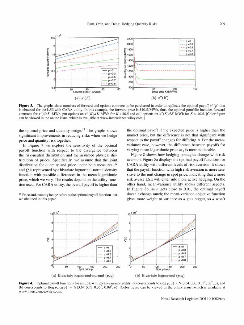
For an LSE with mean-variance utility, the optimal payofffunctions are drawn in Figure 4. They show the tendency ofmean-variance utility to protect against high price and lowquantity. For an illustration of the numbers of contracts to bepurchased in order to obtain payoff x∗(p), see Figure 5. Notethat in our examples the number of options contracts to bepurchased in the optimal portfolio is positive for any strikeprices. This implies that we borrow money from the bank andpurchase a portfolio of options contracts.

Figure 6 compares distribution changes between profitwithout hedging, profit after price hedge14 and profit after

14 Price hedge here means that we add the optimal payoff functionobtained under the assumption of no quantity risk. This is in factequivalent to buying forwards for the average load quantity.



Figure 3. The graphs show numbers of forward and options contracts to be purchased in order to replicate the optimal payoff x∗(p) thatis obtained for the LSE with CARA utility. In this example, the forward price is $40.5/MWh, thus, the optimal portfolio includes forwardcontracts for x ′(40.5) MWh, put options on x ′′(K)dK MWh for K< 40.5 and call options on x ′′(K)dK MWh for K > 40.5. [Color figurecan be viewed in the online issue, which is available at www.interscience.wiley.com.]

the optimal price and quantity hedge.15 The graphs showssignificant improvements in reducing risks when we hedgeprice and quantity risk together.

In Figure 7 we explore the sensitivity of the optimalpayoff function with respect to the divergence betweenthe risk-neutral distribution and the assumed physical dis-tribution of prices. Specifically, we assume that the jointdistribution for quantity and price under both measures P

and Q is represented by a bivariate lognormal-normal densityfunction with possible differences in the mean logarithmicprice, which we vary. The results depend on the utility func-tion used. For CARA utility, the overall payoff is higher than

15 Price and quantity hedge refers to the optimal payoff function thatwe obtained in this paper.

the optimal payoff if the expected price is higher than themarket price, but the difference is not that significant withrespect to the payoff changes for differing p. For the mean-variance case, however, the difference between payoffs forvarying mean logarithmic price m2 is more noticeable.

Figure 8 shows how hedging strategies change with riskaversion. Figure 8a displays the optimal payoff functions forCARA utility with different levels of risk aversion. It showsthat the payoff function with high risk aversion is more sen-sitive to the unit change in spot price, indicating that a morerisk averse LSE will enter into more active hedging. On theother hand, mean-variance utility shows different aspects.In Figure 8b, as a gets close to 0.01, the optimal payoffdoesn’t change much; the mean-variance objective functiongives more weight to variance as a gets bigger, so a won’t

Figure 4. Optimal payoff functions for an LSE with mean-variance utility. (a) corresponds to (log p, q) ∼ N(3.64, 300, 0.352, 302, ρ), and(b) corresponds to (log p, log q) ∼ N(3.64, 5.77, 0.352, 0.092, ρ). [Color figure can be viewed in the online issue, which is available atwww.interscience.wiley.com.]



Figure 5. The graphs show numbers of forward and options contracts to be purchased in order to replicate the optimal payoff x∗(p)that is obtained for the LSE with mean-variance utility. In this example, the forward price is $40.5/MWh; hence, the optimal portfolioincludes the forward contract for x ′(40.5) MWh, put options on x ′′(K)dK MWh for K< 40.5 and call options on x ′′(K)dK MWh forK > 40.5. The upper Panels (a) and (b) correspond to price and load following a bivariate lognormal-normal distribution, and the lower panelscorrespond to price and load following a bivariate lognormal distribution. [Color figure can be viewed in the online issue, which is availableat www.interscience.wiley.com.]

Figure 6. The comparison of profit distribution for an LSE with mean-variance utility for three cases: before hedge, after price hedge, andafter price and quantity hedge, assuming the correlation coefficient between price and load to be 0.7. [Color figure can be viewed in the onlineissue, which is available at www.interscience.wiley.com.]



Figure 7. Sensitivity of the optimal payoff function to divergence between the risk neutral probability measure and the physical probabilitymeasure. The graphs correspond to the case when price and load follow a bivariate lognormal-normal distribution with correlation coefficient0.5. m2 represents the mean of logarithm of price under the risk-neutral probability measure with m2 = 3.64 corresponding to the case P ≡ Q.[Color figure can be viewed in the online issue, which is available at www.interscience.wiley.com.]

affect the optimal payoff function above a certain level andthe objective turns into minimizing variance. However, forsmaller risk aversion, the mean-variance objective functionputs more weights on the mean of profit; LSEs with lowrisk aversion will protect more against the lower spot priceworrying that the expected profit is low from decreased loadwhen spot price is low.

4. CONCLUSION

Price risk and its management in the electricity mar-ket have been studied by many researchers and is wellunderstood. However, price risk should be understood as acorrelated risk with volumetric risk (quantity risk), whichis also significant. Volumetric risk has great impact on theprofit of load-serving entities; therefore, there is a great needfor methodology addressing volumetric risk management.

We discussed financial contracts that allow LSEs to miti-gate volumetric risk: swing options, interruptible contracts,

and weather derivatives. In particular, weather derivativesare widely used to hedge volumetric risks since there arestrong correlations between weather variables and powerloads.

We propose an alternative approach that exploits the highcorrelation between spot prices and loads to construct a volu-metric hedging strategy based on standard power contracts. Ina one-period setting, we obtain the optimal zero-cost portfolioconsisting of bonds, forwards, and options with a contin-uum of strike prices. Also, the paper shows how to replicatethe optimal payoff using available European put and calloptions. The approximation of a payoff function using avail-able options contracts that was shown in this paper can alsobe applied for hedging in markets that have put and calloptions with many different strike prices. The model andmethodology are applicable to other commodity markets andwith different profit functions.

There are more extensions that can be made to the cur-rent model. First, the zero-cost assumption allows the LSE

Figure 8. Optimal payoffs for the case when price and load follow a bivariate lognormal-normal distributions: N(3.64, 300, 0.352, 302, 0.5)under P while the log-price distribution is N(3.66, 0.352) under Q. [Color figure can be viewed in the online issue, which is available atwww.interscience.wiley.com.]



to borrow as much money at time 0 to buy the options con-tracts. Imposing credit limits on the hedging strategy wouldmake the model more realistic. Second, the electricity marketis incomplete, so the risk-neutral probability measure wechoose would not be exactly the same as what the market usesfor pricing. Therefore, a pricing error would exist, which canlead to inefficient hedging. A model that accounts for possibleerrors in choosing the risk-neutral probability measure wouldbe a good extension for applications in the actual electricitymarkets.

REFERENCES

[1] N. Audet, P. Heiskanen, J. Keppo, and I. Vehvilainen, “Model-ing electricity forward curve dynamics in the Nordic market,”Modelling prices in competitive electricity markets, D.W.Bunn (Editor), Wiley Series in Financial Economics.

[2] R.N. Boisvert, P.A. Cappers, and B. Neenan, The benefits ofconsumer participation in wholesale electricity markets, ElectJ 15(3) (2002), 41–51.

[3] G.W. Brown and K.B. Toft, How firms should hedge, RevFinan Stud 15(4) (2002), 1283–1324.

[4] P. Carr and D. Madan, Optimal positioning in derivativesecurities, Quant Finan 1 (2001), 19–37.

[5] D. Caves, K. Eakin, and A. Faruqui, Mitigating price spikesin wholesale markets through market-based pricing in retailmarkets, Elect J 13(3) (2002), 13–23.

[6] H. Chao and R. Wilson, Resource adequacy and market powermitigation via options contracts, UCEI POWER conference,Berkeley, March 2004.

[7] CPUC Order Instituting Rulemaking to Establish Policies andCost Recovery Mechanisms for Generation Procurement andRenewable Resource Development Interim Opinion, DecisionNo. 04-01-050, January 22, 2004.

[8] CPUC Resource Adequacy Proceeding Interim OpinionRegarding Resource Adequacy, Decision No.04-10-035,October 28, 2004.

[9] L. Clewlow and C. Strickland, Energy derivatives: Pricing andrisk management, Lacima Publications, 2000.

[10] D. Duffie, Dynamic asset pricing theory, Princeton UniversityPress, Princeton, 1992.

[11] A. Eydeland and K. Wolyniec, Energy and power risk man-agement: New development in modeling, pricing, and hedging,Willy, 2001.

[12] T.W. Gedra and P.P. Varaiya, Markets and pricing for inter-ruptible electricity power, IEEE Trans Power Syst 8(1) (1993),122–128.

[13] H. Geman, Towards a European market of electricity: Spotand derivatives trading, 2002, available at http://www.nea.fr/html/ndd/investment/session2/geman.pdf.

[14] E. Hirst, Price-responsive demand in wholesale markets: Whyis so little happening? Elect J 14(4) (2002), 25–37.

[15] O. Jaillet, E. Ronn, and S. Tompaidis, Valuation of commoditybased swing options, Working paper, UT Austin, 2001.

[16] K. Kallsen, A utility maximization approach to hedging inincomplete markets, Math Methods Oper Res 50 (1999),321–338.

[17] I. Karatzas and S. Shreve, Methods of mathmatical finance,Springer, New York, 1998.

[18] J. Keppo, Pricing of electricity swing options, J Deriv 11(2004), 26–43.

[19] S. Koekebakker and F. Ollmar, Forward curve dynamics in theNordic electricity market, Manag Finance 31 (2005), 73–94.

[20] Y. Li and P. Flynn, A comparison of price patterns in dereg-ulated power markets, UCEI POWER Conference, Berkeley,March 2004.

[21] R.I. McKinnon, Futures markets, buffer stocks, and incomestability for primary producers, J Polit Econ 75 (1967),844–861.

[22] G. Moschini and H. Lapan, The hedging role of options andfutures under joint price, basis, and production risk, Int EconRev 36(4) (1995).

[23] E. Nasakkala and J. Keppo, Electricity load pattern hedg-ing with static forward strategies, Manag Finan 31(6) (2005),115–136.

[24] J. Rolfo, Optimal hedging under price and quantity uncer-tainty: The case of a cocoa producer, J Poli Econ 88 (1989),100–116.

[25] T.P. Strauss and S.S. Oren, Priority pricing of interruptibleelectricity power with an early notification option, Energy J14(2) (1993), 175–195.

[26] A.C. Thompson, Valuation of path-dependent contingentclaims with multiple exercise decisions over time: The caseof take-or-pay, J Finan Quant Anal 30(2) (1995), 271–293.

[27] G. Unger, Hedging strategy and electricity contract engineer-ing, a dissertation, the Swiss Federal Institute of Technology,Zurich, 2002.

[28] M. Wagner, P. Skantze, and M. Ilic, “Hedging optimizationalgorithms for deregulated electricity markets,” Proceedingsof the 12th Conference on Intelligent Systems Application toPower Systems, 2003.


hedging quantity risks with standard power options in …oren/pubs/i.a.87.pdfhedging quantity risks...

Documents