heavy metals in maltese agricultural soil
TRANSCRIPT

Heavy Metals in Maltese Agricultural Soil
“submitted in partial fulfilment
of the requirements of the
Master of Science in Biochemistry”
Jessica Briffa
2020


Page | ii
The research work disclosed in this publication is partially funded by the
Endeavour Scholarship Scheme (Malta). Scholarships are part-financed
by the European Union - European Social Fund (ESF) -
Operational Programme II –Cohesion Policy 2014-2020
“Investing in human capital to create more opportunities and promote the well-being of society”.
European Union –European Structural and Investment Funds Operational Programme II –Cohesion Policy 2014-2020 “Investing in human capital to create more opportunities and promote the well-being of society.” Scholarships are part financed by the European Union - European Social Funds (ESF) Co-financing rate: 80% EU Funds; 20% National Funds

Page | iii
Acknowledgement
I wish to express my sincere appreciation to my supervisor, Professor Renald Blundell, for the
motivation to start this course, the encouragement and help, throughout the course. My heartfelt
gratitude goes to my co-supervisor Professor Emmanuel Sinagra, for his advice and support,
throughout these two years.
I would like to thank Mr Joseph Grech for helping me understand how to use and interpret the X-
Ray Fluorescence spectrometer and for his help and patience throughout the research journey.
Special thanks go to the individuals who provided me with the soils to analyse since, without their
help, this study would not have been possible. Thanks go to the Department of Agriculture for
their support, primarily to conduct the pilot study.
Last but not least, I would like to express my thanks and gratefulness to my mother, father,
brother, sister-in-law, and Florin, who have been so supportive during these years and have been
there for me throughout it all. I would not have managed without them. Thanks go to my friends
Nicolette Sammut, Stephanie Smith and Maria Calleja for their continuous support and
motivation throughout this journey.

Page | iv
Abstract
Soil pollution has increased over the last few decades due to anthropogenic sources. Heavy
metal pollution has been of great concern since it has been noted that these contaminants
have entered our food chain. High concentration of heavy metals can adversely affect the
health of the public wellbeing. The aim of the study was to evaluate whether i) heavy metals
found in soil are present in high amounts; ii) heavy metals found in soil are present
differently across Malta and Gozo; iii) there are soil limits regulating heavy metals. The soil
samples were analysed with an X-Ray Fluorescence Spectrometer using the sample cup
method. The method of analyses was validated by comparing it to the results obtained in an
external laboratory. The samples were analysed to determine the concentration of heavy
metals, namely aluminium, vanadium, chromium, cobalt, manganese, nickel, copper, zinc,
molybdenum, arsenic, silver, cadmium, selenium, mercury and lead in soil. Samples were
collected from five districts in Malta and from Gozo. A total of 103 samples were collected
and analysed, out of which two samples were collected from organic farms and used as
controls. Samples were analysed in triplicate and an average was calculated. Most of the soil
samples tested showed that the heavy metals found in the soil were observed to be present
at higher concentrations in the South-Eastern District and the Southern Harbour.
Concentrations of the heavy metals tested were mapped out according to district and
localities. The highest concentration of aluminium was found in the Western District at
38106.00 mg/kg. The highest concentration of lead was observed in the Southern Harbour
and was statistically significantly (ρ-value<0.05) different from the rest of the districts with a
concentration of 249.51 mg/kg. Other metals that were found at their highest
concentrations in the Southern Harbour, were copper at 95.15 mg/kg and zinc at 251.33
mg/kg. The heavy metals vanadium at 64.25 mg/kg, chromium at 45.93 mg/kg, manganese
at 586.67 mg/kg, nickel at 21.90 mg/kg and selenium at 15.51 mg/kg, to be observed at their
highest concentrations in the South-Eastern District when compared to the other districts.
The highest concentrations of molybdenum at 12.09 mg/kg, arsenic at 7.93 mg/kg and
cadmium at 30.10 mg/kg were observed in the Northern District. Cobalt was seen with the
highest concentration in the Gozo and Comino District, at 15.83 mg/kg. The Finland and
Dutch standards were used to compare the results observed. Lead was found to exceed the
threshold limits of the Finland standard which is 60 mg/kg and the Dutch standard which is
85 mg/kg. Cadmium was observed to exceed the threshold value of the Finland standard
which is 1 mg/kg and the Dutch standard which is 0.8 mg/kg. The Finland standard
concentration of arsenic is 1 mg/kg, which was much lower than the concentration observed
in the Northern District. Zinc was found to exceed the threshold limits of the Finland
standard which is 200 mg/kg and the Dutch standard value which is 50 mg/kg. The lower
concentration of heavy metals observed in organic farms may be attributed to the lack of
chemical use whereby instead biodiversity is applied to aid in pest and weed reduction.
There is a need for the implementation of methods to address the high concentrations of
heavy metals. Such methods which can be applied include phytoremediation, intercropping
and organic farming.

Page | v
Table of Contents
Chapter 1: Introduction............................................................................................................................ 1
1.1 Soil Formation and Composition .............................................................................................. 2
1.2 Soil Pollution ............................................................................................................................ 7
1.2.1 Point Source Pollution ...................................................................................................... 9
1.2.2 Diffuse Pollution ............................................................................................................. 10
1.3 Source of Pollution ................................................................................................................. 12
1.3.1 Natural Source of Pollution ............................................................................................ 12
1.3.2 Anthropogenic Source of Pollution ................................................................................ 13
1.3.2.1 Livestock and Agriculture Soil Pollution ..................................................................... 15
1.3.2.2 The Impact of Sewage, Waste Production and Disposal on Soil ................................ 18
1.3.2.3 Industrial Activity Pollution ........................................................................................ 22
1.3.2.4 Infrastructures, Transport and Urbanisation ............................................................. 27
1.3.2.5 Fireworks .................................................................................................................... 30
1.3.2.6 Mining Activities ......................................................................................................... 32
1.3.2.7 Warfare Actions ......................................................................................................... 33
1.4 Soil Pollutants ......................................................................................................................... 34
1.4.1 Inorganic Ions ................................................................................................................. 35
1.4.1.1 Heavy Metals and Metalloids ..................................................................................... 35
1.4.1.2 Anions – Phosphorus and Nitrogen ........................................................................... 36
1.4.2 Organic Pollutants .......................................................................................................... 38
1.4.2.1 Hydrocarbons ............................................................................................................. 38
1.4.2.2 Persistent Organic Pollutants: Polychlorinated and Polybrominated pollutants. ..... 40
1.4.2.3 Pesticides .................................................................................................................... 42
1.4.2.3.1 Organochlorine Insecticides ................................................................................. 42
1.4.2.3.2 Organophosphorus Insecticides ........................................................................... 43
1.4.2.3.3 Carbamate Insecticides ........................................................................................ 43
1.4.2.3.4 Pyrethroid Insecticides ......................................................................................... 44
1.4.2.3.5 Neonicotinoids ..................................................................................................... 44
1.4.2.3.6 Plant Growth Regulators – Phenoxy Herbicides .................................................. 45
1.4.2.3.7 Anticoagulant Rodenticides ................................................................................. 46
1.4.2.3.8 Emerging Organic Pollutants ................................................................................ 46
1.4.3 Organometallic Compounds .......................................................................................... 48
1.4.4 Radionuclides ................................................................................................................. 48

Page | vi
1.4.5 Gaseous Pollutants ......................................................................................................... 50
1.4.6 Pathogenic Microorganisms ........................................................................................... 50
1.4.7 Nanoparticles ................................................................................................................. 51
1.5 Heavy Metals .......................................................................................................................... 52
1.5.1 Properties of Heavy Metals and Metalloids ................................................................... 52
1.5.2 Entry, Transportation and Effects of Heavy Metals into the Ecosystem ....................... 54
1.5.3 Soil Contamination ......................................................................................................... 54
1.5.4 The Fate of the Heavy Metals in Soil .............................................................................. 56
1.5.5 Uptake of Metals by Plants and Entry into the Food Chain ........................................... 58
1.6 Metal ions .............................................................................................................................. 59
1.6.1 Aluminium ...................................................................................................................... 59
1.6.2 Vanadium ....................................................................................................................... 63
1.6.3 Chromium ....................................................................................................................... 64
1.6.4 Manganese ..................................................................................................................... 67
1.6.5 Cobalt ............................................................................................................................. 68
1.6.6 Nickel .............................................................................................................................. 69
1.6.7 Copper ............................................................................................................................ 71
1.6.8 Zinc ................................................................................................................................. 73
1.6.9 Molybdenum .................................................................................................................. 74
1.6.10 Arsenic ............................................................................................................................ 75
1.6.11 Silver ............................................................................................................................... 78
1.6.12 Cadmium ........................................................................................................................ 79
1.6.13 Selenium ......................................................................................................................... 81
1.6.14 Mercury .......................................................................................................................... 83
1.6.15 Lead ................................................................................................................................ 86
1.7 Carcinogens ............................................................................................................................ 87
1.8 Aim and Objectives ................................................................................................................ 88
Chapter 2: Materials and Methods ....................................................................................................... 90
2.1 Pilot study .............................................................................................................................. 91
2.2 Sample Collection ................................................................................................................... 94
2.3 Reference control using organic farms .................................................................................. 96
2.4 Sample Preparation and Analysis ........................................................................................... 97
2.5 XRF instrumentation and sample cup preparation ................................................................ 98
Chapter 3: Results ............................................................................................................................... 101
3.1 Pilot Study ............................................................................................................................ 102
3.1.1 Repetitive sampling to test consistency....................................................................... 102
3.1.2 Comparison of XRF and ICP-MS values ........................................................................ 103

Page | vii
3.2 Results obtained from XRF spectrometer ............................................................................ 109
3.2.1 Macronutrients Group ................................................................................................. 115
3.2.2 Micronutrients Group .................................................................................................. 118
3.2.2.1 Manganese ............................................................................................................... 120
3.2.2.2 Copper ...................................................................................................................... 121
3.2.2.3 Molybdenum ............................................................................................................ 123
3.2.2.4 Zinc ........................................................................................................................... 124
3.2.3 Halogens Group ............................................................................................................ 126
3.2.4 Heavy Metals Group ..................................................................................................... 126
3.2.4.1 D-block Elements ..................................................................................................... 127
3.2.4.1.1 Lead .................................................................................................................... 130
3.2.4.1.2 Vanadium ........................................................................................................... 131
3.2.4.1.3 Chromium .......................................................................................................... 133
3.2.4.1.4 Cadmium ............................................................................................................ 134
3.2.4.1.5 Nickel .................................................................................................................. 136
3.2.4.1.6 Cobalt ................................................................................................................. 137
3.2.4.1.7 Arsenic ................................................................................................................ 139
3.2.4.2 P-block elements ...................................................................................................... 140
3.2.4.2.1 Aluminium .......................................................................................................... 142
3.2.4.2.2 Selenium............................................................................................................. 144
3.2.4.3 S-block elements ...................................................................................................... 145
3.2.4.4 F-Block elements ...................................................................................................... 147
3.2.5 Localities and districts most affected by the heavy metals ......................................... 148
3.3 Control sample results ......................................................................................................... 152
Chapter 4: Discussion .......................................................................................................................... 155
4.1 Comparison in the pilot study .............................................................................................. 156
4.2 XRF peaks ............................................................................................................................. 157
4.3 Heavy Metals Found in each District and Locality ............................................................... 159
4.3.1 Aluminium .................................................................................................................... 159
4.3.2 Manganese ................................................................................................................... 159
4.3.3 Lead .............................................................................................................................. 160
4.3.4 Copper .......................................................................................................................... 162
4.3.5 Vanadium ..................................................................................................................... 163
4.3.6 Cadmium ...................................................................................................................... 163
4.3.7 Chromium ..................................................................................................................... 164
4.3.8 Arsenic .......................................................................................................................... 165
4.3.9 Cobalt ........................................................................................................................... 166

Page | viii
4.3.10 Nickel ............................................................................................................................ 167
4.3.11 Molybdenum ................................................................................................................ 168
4.3.12 Selenium ....................................................................................................................... 168
4.3.13 Zinc ............................................................................................................................... 168
4.4 Controls ................................................................................................................................ 169
4.5 Limitations and Recommendations for Future Work .......................................................... 170
4.5.1 Practices to Target High Levels of Heavy Metal Concentrations ................................. 172
4.5.2 Phytoremediation ........................................................................................................ 173
4.5.3 Intercropping ................................................................................................................ 174
4.5.4 Organic Farming ........................................................................................................... 176
4.6 Conclusion ............................................................................................................................ 177
Chapter 5: Bibliography ....................................................................................................................... 178
Chapter 6: Appendices ........................................................................................................................ 199

Page | ix
List of Tables
Table 1: Nuclear accidents around the world (Battist and Peterson, 1980; McLaughlin, Jones and
Maher, 2012; Union of Concerned Scientists, 2013). ............................................................................ 49
Table 2: GPS Coordinates of Għammieri Samples ................................................................................. 91
Table 3: XRF mean value compared to ICP-MS values in ppm............................................................. 103
Table 4: Binomial test ρ-values for XRF vs ICP-MS scores .................................................................... 104
Table 5: Southern Harbour Samples .................................................................................................... 110
Table 6: Northern Harbour Samples .................................................................................................... 110
Table 7: South-Eastern Samples ........................................................................................................... 111
Table 8: Western Samples .................................................................................................................... 112
Table 9: Northern Samples .................................................................................................................. 113
Table 10: Gozo and Comino Samples ................................................................................................... 113
Table 11: Mean Values for Macronutrients ......................................................................................... 116
Table 12: Mean Value of Micronutrients ............................................................................................. 118
Table 13: Mean element value of D-block elements ........................................................................... 128
Table 14: Mean element value of P-block elements ........................................................................... 140
Table 15: Mean element values of S-block elements .......................................................................... 145
Table 16: Mean element value for F-block elements .......................................................................... 147
Table 17: Binomial analysis between mean district value and Control 1. ........................................... 153
Table 18: Binomial analysis between mean district value and Control 2 ............................................ 154

Page | x
List of Figures
Figure 1: Different Soils which can be found in Malta, Gozo and Comino (MALSIS, 2004). .................... 5
Figure 2: Land Use and Cover of Malta, Gozo and Comino (European Commission, 2019). ................. 14
Figure 3: Locations of fireworks factories (grey spots) and mineral and stone quarries (black shading)
(European Commission, 2019) ............................................................................................................... 15
Figure 4: Contamination sites in Malta and Gozo (Marine Strategy Framework Directive, 2016) ........ 27
Figure 5: Għammieri fields and Sample Locations ................................................................................. 92
Figure 6: Map of sampling method ........................................................................................................ 95
Figure 7: Graphical Image of Malta, Gozo and Comino using NUTS Classification according to the
LAU1 (NSO, 2017). .................................................................................................................................. 96
Figure 8: Positive correlation co-efficient of all the elements between XRF and ICP-MS measurements
in mg/kg ............................................................................................................................................... 105
Figure 9: Positive linear correlation co-efficient between equipment measured in mg/kg for ......... 106
Figure 10: Positive linear correlation co-efficient between equipment measured in mg/kg for A)
nickel; B) copper; C) zinc ...................................................................................................................... 107
Figure 11: Zero linear correlation co-efficient for A) mercury; B) chromium ...................................... 108
Figure 12: Google Earth Pro Map illustrating the areas of the 101 samples ....................................... 109
Figure 13: Mean element concentrations in ppm in each district ....................................................... 115
Figure 14: Macronutrient's concentrations in each district ................................................................. 116
Figure 15: Macronutrient's concentrations excluding calcium in each district ................................... 117
Figure 16: Micronutrient's concentrations in each district .................................................................. 119
Figure 17: Micronutrient's concentrations excluding iron in each district .......................................... 119
Figure 18: Manganese concentrations by district ................................................................................ 120
Figure 19: Manganese concentrations by locality sampled ................................................................. 121
Figure 20: Copper concentrations by district ....................................................................................... 122
Figure 21: Copper concentrations by localities sampled ..................................................................... 122
Figure 22: Molybdenum concentrations by district ............................................................................. 123
Figure 23: Molybdenum concentrations by localities sampled ........................................................... 124
Figure 24: Zinc concentrations by districts .......................................................................................... 125
Figure 25: Zinc concentrations by locality............................................................................................ 125
Figure 26: Halogens concentrations in each district ............................................................................ 126
Figure 27: D-block concentrations in each district .............................................................................. 128
Figure 28: D-block concentrations in each district excluding titanium................................................ 129
Figure 29: D-block concentrations in each district excluding titanium, zirconium and lead ............... 129
Figure 30: Lead concentrations by district ........................................................................................... 130
Figure 31: Lead concentrations by localities sampled ......................................................................... 131
Figure 32: Vanadium concentrations by district ................................................................................. 132
Figure 33: Vanadium concentrations by localities sampled ................................................................ 132
Figure 34: Chromium concentrations by district ................................................................................. 133
Figure 35: Chromium concentrations by localities sampled ................................................................ 134
Figure 36: Cadmium concentrations by district ................................................................................... 135
Figure 37: Cadmium concentrations by localities sampled ................................................................. 135
Figure 38: Nickel concentrations by district ......................................................................................... 136
Figure 39: Nickel concentrations by localities sampled ....................................................................... 137
Figure 40: Cobalt concentrations by district ........................................................................................ 138
Figure 41: Cobalt concentrations by localities sampled ...................................................................... 138
Figure 42: Arsenic concentrations by district....................................................................................... 139
Figure 43: Arsenic concentrations by localities sampled ..................................................................... 140

Page | xi
Figure 44: P-block element concentrations in each district................................................................. 141
Figure 45: P-block concentrations in each district excluding aluminium and silicon .......................... 141
Figure 46: Aluminium concentrations by district ................................................................................. 143
Figure 47: Aluminium concentrations by localities sampled ............................................................... 143
Figure 48: Selenium concentrations by district ................................................................................... 144
Figure 49: Selenium concentrations by locality ................................................................................... 145
Figure 50: S-block concentrations in each district ............................................................................... 146
Figure 51: S-block concentrations in each district excluding sodium .................................................. 147
Figure 52: F-block concentrations in each district ............................................................................... 148
Figure 53: Elements according to percentage concentration by locality ............................................ 149
Figure 54: Percentage concentration of heavy metals by district ....................................................... 150
Figure 55: Percentage of heavy metals found in each district ............................................................. 151
Figure 56: Percentage of heavy metals found in each district excluding aluminium .......................... 152

Page | xii
Appendix 1: Shapiro Wilk test ...................................................................................................... 200
Appendix 2: One-Way ANOVA and Kruskal-Wallis test ............................................................ 201
Appendix 3: ICP-MS Results ........................................................................................................... 206
Appendix 4: Shapiro-Wilk Test ...................................................................................................... 208
Appendix 5: One-Way ANOVA Test and Kruskal-Wallis Test (Districts) ............................... 209
Appendix 6: Sample A ...................................................................................................................... 214
Appendix 7: Sample B ...................................................................................................................... 215
Appendix 8: Sample C ...................................................................................................................... 216
Appendix 9: Sample D ...................................................................................................................... 217
Appendix 10: Sample E .................................................................................................................... 218
Appendix 11: Southern Harbour Samples ................................................................................... 219
Appendix 12: Northern Harbour Samples ................................................................................... 220
Appendix 13: South-Eastern District Samples ............................................................................ 221
Appendix 14: Western District Samples ............................................................................................. 222
Appendix 15: Northern District Samples ..................................................................................... 223
Appendix 16: Gozo and Comino District ...................................................................................... 224
Appendix 17: Example of XRF graph with a chromium peak but a 0 ppm value ................. 225

Page | xiii
List of Abbreviations
ATP Adenosine Triphosphate
ATSDR Agency for Toxic Substances and Disease Registry
COPD Chronic Obstructive Pulmonary Disease
DDT Dichlorodiphenyltrichloroethane
DNA Deoxyribonucleic acid
EDXRF Energy dispersive X-ray fluorescence
EU European Union
GPS Global positioning system
HCHs Hexachlorocyclohexanes
HDL High-Density Lipoproteins
IAEA International Atomic Energy Agency
IARC International Agency of Research on Cancer
ICP-MS Inductively coupled plasma mass spectrometry
ICAO International Civil Aviation Organization
IPPC Integrated Pollution Prevention and Control
ISRIC International Soil Reference and Information Centre
LAU1 Local administrative units, level 1
NSO National Statistics Office
NUTS Nomenclature of Territorial Units for Statistics
PAHs Polycyclic Aromatic Hydrocarbons
PBBs Polybrominated Biphenyls
PCBs Polychlorinated Biphenyls
PCDDs Polychlorinated Dibenzidioxins
PCDFs Polychlorinated Dibenzoflurans
PCPs Personal Care Products
PM Particulate Matter
PPCPs Pharmaceuticals and Personal Care Products
ppm Parts per million
RNA Ribonucleic acid
TCDD 2,3,7,8-Tetrachlorodibenzo-p-dioxin
U.S. United States
UNDP United Nations Development Programme
UNEP United Nations Environment Programme
WHO World Health Organisation
XRF X-ray fluorescence

Page | 1
Chapter 1: Introduction

Page | 2
1.1 Soil Formation and Composition
Soil formation is a time-consuming progressive process and is a precious natural resource.
It is known as pedogenesis and is dependent on a combination of processes occurring at the
top of the soil, which includes physical, anthropogenic, chemical and biological processes.
Soil is composed of weathered rocks which are the mineral particles, together with water, air
and organic matter, all of which are easily affected by anthropogenic activity. The minerals
present in the soil, which are derived from the weathered rocks, experience changes where
secondary minerals are formed together with other sporadically water-soluble compounds.
These elements are translocated from one region of soil to another through animal activity
and by water (Environment & Resources Authority, 2016a). All the translocation and
transformation of the minerals throughout the soil causes distinct soil horizons
(Environment & Resources Authority, 2016a; Rodriguez-Eugenio, McLaughlin and Pennock,
2018).
The physical properties of soil consist of six characteristics which include the colour,
texture, consistency, structure, horizonation and bulk density, while the soil chemical
properties consist of two characteristics, namely the soil’s pH and its cation exchange
capacity.
Soil horizons are developed during soil genesis, which produces different layers that vary
in colour and texture compared to the layer above and below. The soil colour depends on
three properties which comprise of the amount of iron oxide found in the soil, the amount
of organic matter and the amount of moisture present. The texture depends upon the
quantities of the soil “separates” which consist of sand, clay and silt. Sand and silt do not
play any role in the soil since they do not partake in the mineral or water retention. Clay is
the only separate that contributes to the soil, by attracting water and ions due to its surface

Page | 3
charge. Soil structure can be defined as the aggregation of the soil separates into discrete
structural units known as “peds”, which can be found in repeating patterns. Pores can be
present between the structural units where air and water can pass. The structural shape in
the soil horizon describes the type of soil structure, and the proportion of soil weight
compared to the volume describes the bulk density of the soil. The last characteristic of soil
is consistency. Consistency depends on the moisture content present in the soil. It describes
the effortlessness of crushing an individual ped. Soil consistency can be divided into three
types and is described as moist soil, wet soil or dry soil (Brady, 1990).
Soils are essential for agricultural purposes as they are the medium through which crops
are grown. Natural causes such as heavy storms and winds may lead to soil erosion and can
sometimes displace the amounts of soil. Soil erosion displaces mainly the top horizon of the
soil, but sometimes the whole profile is compromised causing issues when coming to food
security, biodiversity and climate change desertification (Environment & Resources
Authority, 2016a; Rodriguez-Eugenio, McLaughlin and Pennock, 2018).
Malta and its sister islands Gozo and Comino, have a total area of 316 km2 of land (NSO,
2019). Between the islands there is 41% of agricultural land, where Gozo and Comino have
46.9% of agricultural land and Malta has 35.2% (NSO, 2019). Forage plants are the popular
component in arable land in both Malta and Gozo, followed by vegetables and fallow land.
Vineyards, citrus, fruit and berry plantations and olive plantations are found to be the top
permanent crops (NSO, 2019). Farming land is found scattered all over the islands, and each
area has a different type of soil with different characteristics and different elements.
The Maltese Islands have different types of soils regardless of the archipelago’s small
territorial extent. D.M. Lang was the first person to create a map of Malta’s soil in 1956-1957

Page | 4
(Sammut, 2005). He established that the different soils result from local geology, are
extremely calcareous and are chemically closely correlated (Sammut, 2005).
Maltese soil has a distinctive pattern that is very intricate. A single field may contain
different soil types, and the nearby agricultural land may have a different type. Different soil
types have come about due to three prime human factors which are intertwined and are (i)
urbanisation; (ii) excavated soil transportation from construction sites (Fertile Soil
(Preservation) Act, 1973); and (iii) the replenishment of shallow or eroded soils or soil that
has been subjected to human interference (Sammut, 2005).
The archipelago’s soils are slightly-moderately alkaline, and two-thirds of the island’s soils
are problematic to work since they have a high clay content which may amount up to 48%.
On the other hand, these soils have a higher water filtration capacity and a greater nutrient
retention capacity (Malta Environment & Planning Authority state of the environment report,
2005).
A map was drawn up to show the different types of soils due to the different types of rock
present which influences the soil’s minerals. Most of the land can be seen to be globigerina
limestone (Figure 1).

Page | 5
Figure 1: Different Soils which can be found in Malta, Gozo and Comino (MALSIS, 2004).

Page | 6
A variety of soil biophysical functions include several properties such as nutrient cycling,
water dynamics, and filtering plus buffering, physical support and physical stability to the
plants’ system as well as human structures, habitat for organisms and biodiversity
promotion. For soil to deliver its functions, the condition of the soil’s properties has to be
taken into account (Hatfield, Sauer and Cruse, 2017).
Soil function has led to a degradation of the soil, due to agricultural practices that are
being used today to increase the amount of crop yield being grown. The soil has degraded
due to wind and tillage, erosion due to overwatering, salinization and sodification, organic
carbon reduction, the decline in soil biodiversity and most of all through soil contamination
(MacEwan, Dahlhaus and Fawcett, 2012; Baishya, 2015). There are three types of soil
degradation which are known as physical, chemical and biological (Baishya, 2015).
Physical degradation is caused by tillage and heavy machinery which leads to a restriction
in root growth, limits the amount of water and air kept by the soil, and structural
deterioration of the soil (Baishya, 2015).
The main culprits of chemical degradation are fertilizers, pesticides and the quality and
management of water used. These factors lead to a reduction in water availability in the soil,
structural deterioration of soil, environmental pollution and toxic salt effects (Baishya,
2015).
Biological degradation is caused by reduced biodiversity and organic matter depletion
affecting the carbon cycling in the soil, which has an impact on the physical degradation of
soil and nutrient and water regulation processes (Baishya, 2015).

Page | 7
1.2 Soil Pollution
The term “soil pollution” refers to the presence of an element or chemical that is found in
soils that do not have the element or chemical usually present, or found at a higher
concentration level than usual, which can cause adverse effects on any organism. Since soil
pollution is not something that can be seen by the naked eye, it makes it even more
dangerous. A variety of contaminants are continually being evolved as a result of
agrochemical use and industrialisation (Rodriguez-Eugenio, McLaughlin and Pennock, 2018).
Soil contamination and soil pollution have sometimes been used interchangeably, though
they do not have the same meaning. Soil contamination is used when describing the
concentration of a substance or chemical which is present at a higher concentration than it
would have been found typically and does not cause any harm. On the other hand, soil
pollution refers to the presence of substances or chemicals that are not usually found
naturally and are present at a high concentration which will cause adverse effects to an
organism (Rodriguez-Eugenio, McLaughlin and Pennock, 2018). Determining a threshold may
vary from country to country. When taking heavy metals and metalloids into consideration,
other factors have to be seen, such as the rate of weathering of rocks which may release a
more significant number of heavy metals into the soil. Other factors such as threshold
values, screening values, target values, acceptable concentrations, intervention values and
many more can affect the threshold value between countries (Carlon, 2007; Jennings, 2013;
Rodriguez-Eugenio, McLaughlin and Pennock, 2018).
Industrialisation, has had a significant impact on the utilisation of earth’s natural
resources over the last hundred years, which has aggravated environmental pollution,
together with agriculture and livestock, mining and wars. The environment has been
polluted by a variety of contaminants such as organic and inorganic ions, radioactive

Page | 8
isotopes, organometallic compounds, nanoparticles and also gaseous pollutants (Bundschuh
et al., 2012; C.H. Walker, R.M. Sibly, S.P. Hopkin, 2012; Gautam et al., 2016; Rodriguez-
Eugenio, McLaughlin and Pennock, 2018). Unfortunately, Malta’s soils have been
contaminated through a variety of factors such as industrial waste dumps; quarries; lead
shot; car and plane exhaust emission; acid rain; agriculture chemicals such as pesticides,
snail and rat poison; and manure application. Soils also have been eroded through salt,
water and the addition of nutrients (Sammut, 2005; MacEwan, Dahlhaus and Fawcett, 2012).
All these contaminations have added compounds and elements to the soil that are not
naturally found and which can cause harm to the vegetation growing, along with the end-
user of the product. Such elements are heavy metals. Zinc has been found in excess at 200
mg/kg in 7% of Maltese soils. Lead concentration was found in 25% of the soils with values
of more than 100 mg/kg. 3% of the soils have been seen to have copper which exceeded
100mg/kg (Malta Environment & Planning Authority state of the environment report, 2005).
Soil pollution has been recognised as the third most significant risk to soil functions in
Eurasia and Europe and is an alarming problem. It is found to be the fourth and fifth risk to
soil functions in North Africa and Asia respectively, seventh and eighth in Northwest Pacific
and North American while ninth in sub-Saharan Africa together with Latin America
(Rodriguez-Eugenio, McLaughlin and Pennock, 2018).
In the 1990s, the International Soil Reference and Information Centre (ISRIC) together
with the United Nations Environment Programme (UNEP), had done a global estimation of
the total amount of soil that was polluted which amounted to an average of 22 million
hectares (Rodriguez-Eugenio, McLaughlin and Pennock, 2018). The amount of soil polluted
was then thought to be an underestimation of the real amount of soil pollution. Some
countries have investigated their soil pollution, which has brought about informative data.

Page | 9
However, low-income countries have not reported any data till this time which does not
reflect the real data of soil pollution across the world (Rodriguez-Eugenio, McLaughlin and
Pennock, 2018). In the European Economic Area, together with West Balkans, around three
million possibly polluted sites are present (Van Liedekerke et al., 2014). The Chinese
Environmental Protection Ministry has also acknowledged that 16.1% of the Chinese soils
exceed the general pollution limits, along with 19% of agricultural soils where confirmed as
polluted. Australia has confirmed that they have an estimation of 80,000 contaminated sites
(Department of Environment and Conservation, 2010; CCID, 2015). The United States (U.S.)
of America has confirmed that they have more than 1,300 contaminated soils (Rodriguez-
Eugenio, McLaughlin and Pennock, 2018).
Numerous countries, have implemented or are in the process of implementing national
regulations to safeguard their soils, thus preventing pollution and tackling significant
problems of contamination. One of the main topics discussed during the Estonian
Presidency, in the second half of 2017 of the Council of the European Union, was soil. Soil
was discussed concerning food production and its vital role (Rodriguez-Eugenio, McLaughlin
and Pennock, 2018).
Soil pollution can be caused by a single identifiable source, called point-source pollution,
such as industrial effluent and shipwrecks. On the other hand, soil pollution can be caused
by mostly dispersed and detached sources of pollution, called non-point source pollution or
diffuse pollution such as urban runoffs (Li, 2014; Tarazona, 2014).
1.2.1 Point Source Pollution
Point-source pollution is mainly caused through anthropogenic activities which release
pollutants into the soil, and the source is identified effortlessly. It is quite widespread in

Page | 10
urban areas. Activities which lead to point-source pollution comprises of factory sites,
uncontrolled landfills, waste disposal, and extreme use of agrochemicals, mining and
smelting which are conducted using inadequate environmental guidelines. These usually are
a source of heavy metal contamination in many parts all over the world (Mackay et al., 2013;
Lu et al., 2015; Strzebońska, Jarosz-Krzemińska and Adamiec, 2017). Oil spills are a source of
aromatic hydrocarbon pollution, together with toxic metal. Examples of oil spills around the
world are the Greenland oil tanks, whereby these tanks used small amounts of oil daily,
which caused an exceeded release of aromatic hydrocarbons and toxic metal compared to
the Danish environmental quality criteria (Fritt-Rasmussen et al., 2012). In Tehran, there was
an accidental leakage of oil from the oil refinery storage tanks, which caused a release in
aliphatic hydrocarbons (Pourang and Noori, 2014; Bayat et al., 2016). Old landfills sometimes
had waste disposed of which were not controlled or not disposed of properly, including but
not limited to batteries, medicines and radioactive waste (Karnchanawong and
Limpiteeprakan, 2009; Baderna et al., 2011; Swati et al., 2014). High concentrations of
polycyclic aromatic hydrocarbons, heavy metals and other elements, are found at high
concentrations in the soils that are near roads due to road dust, traffic emission, domestic
emission, industrial emission, weathering of pavements and building surface and so on (Wei
and Yang, 2010; Hua Zhang et al., 2015; Kumar, Kothiyal and Saruchi, 2016; Kim et al., 2017).
Sewage sludge and wastewater not disposed of properly are also classified as point-source
pollutants (Marttinen, Kettunen and Rintala, 2003; Tikilili and Nkhalambayausi-Chirwa, 2011;
Kalmykova et al., 2013)
1.2.2 Diffuse Pollution
Before pollutants are transferred directly to the soil such as point-source pollution,
diffuse pollution transpires. Where released, transformation and dilution of the pollutants

Page | 11
transpire in other media (Rodriguez-Eugenio, McLaughlin and Pennock, 2018). Diffuse
pollution may be harder to track, analyse and restrict its spatial extent, as it comprises of the
transfer of pollutants through the air-soil-water systems. Thus a sophisticated analysis is
needed involving these three systems (release, transformation and dilution) to sufficiently
evaluate the type of pollution (Geissen et al., 2015).
Source of diffuse pollution are (i) uninhibited waste disposal and contaminated sewages
expelled in and near catchments; (ii) nuclear power activities; (iii) weapons activities; (iv)
sewage sludge application on lands; (v) flooding; (vi) soil erosion; (vii) tenacious organic
pollutants; and (viii) agricultural use of fertilizers, manure and pesticides, which add heavy
metals, higher concentrations of nutrients and agrochemicals. Human health is severely
impacted by diffuse pollution and additionally impacts the environment. Severity of the
effect and extent of the impaction, are largely not known (Rodriguez-Eugenio, McLaughlin
and Pennock, 2018). The soils’ top layer is enriched by many pollutants due to atmospheric
deposition from both natural and anthropogenic pollution (Steinnes et al., 1997; Blaser et
al., 2000; Steinnes, Berg and Uggerud, 2011).
Due to the Chernobyl bomb in 1986, radionuclides are present at a high concentration in
the northern hemisphere compared to background levels, and the radionuclides will be
present for many centuries. Since there are different sources of pollution, new methods are
needed to measure and monitor the atmospheric deposition processes together with the
degree of diffuse pollution (Fesenko et al., 2007). After the immediate effect of the atomic
bombs of Hiroshima and Nagasaki, which included the plutonium in the bomb to undergo
fission, an enormous amount of energy have been released. The energy released created a
blinding flash together with temperatures growing to 10 million degrees Celsius. The
electromagnetic radiation then formed a fireball where the wind created from the blast,
destroyed everything in its wake. The extreme temperatures from the radiation burnt

Page | 12
everything. The detonation created a radioactive dust which descended into the
surrounding area. Currents of wind and water carried the radioactive dust further out
from the explosion which then contaminated more soils, water and the entire food chain.
Radionuclides have been present ever since the Chernobyl accident, atomic bombs and
testing of nuclear weapons by the military have occurred (The Committee for the
Compilation of Materials on Damage Caused by the Atomic Bombs in Hiroshima and
Nagasaki, 1981).
1.3 Source of Pollution
As previously stated, there are two types of pollution sources; natural and anthropogenic
sources.
1.3.1 Natural Source of Pollution
Soil pollution should take into consideration the baseline of the soil depending on the
pedo-geochemical fraction together with the dynamics of the environment which formed
that particular soil (Horckmans et al., 2005; Paye, Mello and Melo, 2012; Rodriguez-Eugenio,
McLaughlin and Pennock, 2018). Baseline values, at any given point in the superficial
environments, indicates the value of the genuine content of the element. Background values
show the geogenic natural content of the element (Salminen and Gregorauskiene, 2000;
Reimann, Filzmoser and Garrett, 2005). Concentrations of heavy metals in soils, depending
on the natural difference in the trace metal concentration in the parent rock, can differ from
two to three orders of magnitude (National Research Council, 1977). Many parent rocks are
natural sources of several heavy metals together with other elements including
radionuclides. The volcanic rock contain arsenic, thus weathering of volcanic rock increases
the amount of arsenic (Albanese et al., 2007).

Page | 13
Volcanic eruptions, forest fires, meteorites and dust storms are natural events that cause
natural pollution where several toxic elements such as polycyclic aromatic hydrocarbons and
heavy metals are discharged into the environment. Volcanic soil samples had been tested
around the world, showing that they had high concentrations of heavy metals especially
mercury, together with elements such as chromium, arsenic, nickel, zinc and copper. This
was seen when testing soils on the islands of Réunion and Hawaii, where volcanoes are
found. The elements were present due to the erosion of the parent material which had
these elements as part of its natural geochemical origin. Findings of these elements in high
amounts proved that volcanic eruptions cause a higher amount of the element, in both the
atmosphere and the surrounding soils (Varekamp and Buseck, 1986; Dœlsch, Saint Macary
and Van de Kerchove, 2006; Peña-Rodríguez et al., 2012; Fiałkiewicz-Kozieł et al., 2016).
Polycyclic aromatic hydrocarbons can be found in the soil through cosmic dust from
meteorites that had landed in the area, (Basile, Middleditch and Oró, 1984; Wing and Bada,
1991) or through diagenetic alteration developments of waxes found in the organic matter
of soil (Trendel et al., 1989).
1.3.2 Anthropogenic Source of Pollution
Anthropogenic activity in recent years has increased and resulted in soil pollution all over
the world. Anthropogenic pollution can be caused intentionally such as the use of herbicides,
use of untreated wastewater for irrigation, fertilizer; or sewage sludge land application. It
can also be caused unintentionally by oil spills and landfill leaching (Rodriguez-Eugenio,
McLaughlin and Pennock, 2018).
Anthropogenic sources of soil pollution include livestock and agriculture; sewage and
waste production and disposal; industrial activity; infrastructure, transport and urbanisation;
fireworks; mining and warfare.

Page | 14
The major part of Malta’s industrialisation covers the Southern Harbour, Northern
Harbour and South-Eastern District (Figure 2). Ports, airports, construction sites and waste
sites are labelled on the map. Firework factories and hard stone quarries can be found
dispersed mainly around Malta, with the highest concentration of activity around the whole
island, though concentrated in South-Eastern, Western and Northern District (Figure 3).
Figure 2: Land Use and Cover of Malta, Gozo and Comino (European Commission, 2019).

Page | 15
Figure 3: Locations of fireworks factories (grey spots) and mineral and stone quarries (black shading) (European Commission, 2019)
1.3.2.1 Livestock and Agriculture Soil Pollution
The causes of soil pollution through agriculture and livestock activity can be associated to
the use of pesticides and herbicides, livestock wastes, amendments with solid waste, using
untreated wastewater or poor quality water for crop irrigation, and over fertilisation
(Rodriguez-Eugenio, McLaughlin and Pennock, 2018).
Most farmers add fertilizers and manure to the soils in excessive amount, thus providing
too much nitrogen and phosphorous to the soil (Kanter, 2018). This was seen in the
application of fertilizers in the North China Plain, which had increased drastically, particularly
in the greenhouse vegetable production systems. Northeast China has also mismanaged
fertilizers in agriculture, which has contributed to environmental damage from diffuse
pollution, thus causing alarm, both nationally and internationally (Ju et al., 2007).

Page | 16
Excess fertilizer in the soil can result in the heavy metal build-up, an increase of soil
salinity, and accumulation of nitrogen which is a potential hazard to humans and water
eutrophication. Green gas emissions may cause the extra nitrogen found in the soil to be lost
to the atmosphere, while eutrophication of nearby water sources may be the cause of an
excess of phosphorous. Apart from the diffuse pollution of nitrogen and phosphorous
caused by fertilizers, fertilizers are also a source of heavy metals and natural radionuclides.
These metals and radionuclides are mercury, cadmium, arsenic, lead, nickel, copper, 238
uranium, 232 thallium and 210 polonium. This shows that fertilisers should not be added in
excess (Stewart et al., 2005; Savci, 2012).
Waste of livestock production is another cause of point source pollution if not disposed of
correctly. Animal manure has increased in its use as it is considered as an essential source of
nutrients for the soil and plants. Even though it is of importance to agriculture, there is
evidence that the use of animal manure may increase heavy metals, veterinary antibiotic
residues and pathogens into the soil which may cause antimicrobial-resistant bacteria to
increase in soils. (Rodriguez-Eugenio, McLaughlin and Pennock, 2018). The microorganisms
present in the urine and faeces, can be non-pathogenic or pathogenic to both humans and
animals. Microorganisms that are found in the soil will also be negatively affected by
livestock waste. Medicines given to the livestock is then excreted. These have tendencies to
be lipolytic which do not degrade quickly, thus causing the medical substance to remain in
the manure, which will later be used as fertilizer and thus end up in the soil. (Halling-
Sørensen et al., 1998; Haibo Zhang et al., 2015; Manyi-Loh et al., 2016). In Liaoning China,
pigs and poultry are given feed with a high amount of zinc and copper. On testing soil
treated with manure, it was found that there was an increased amount of copper and zinc in
the soil, due to these metals being added to the poultry and pig feeds. Apart from copper

Page | 17
and zinc, arsenic can be present in poultry health products which will then be excreted in
their manure (Jiang, Dong and Zhao, 2011; Wuana and Okieimen, 2011).
Pesticides have been used for a long time to preserve the crops and to have a large crop
yield. The word “pesticides” includes a range of compounds. (Rodriguez-Eugenio,
McLaughlin and Pennock, 2018). Pesticides and their transformation products can be
grouped into hydrophobic, bioaccumulative and persistent groups, which are firmly bound
to the soil such as lindane, endrin and organochlorine Dichlorodiphenyltrichloroethane
(DDT). Most of these are banned but can still be found in the soils. They can also be grouped
into polar pesticides which include herbicides, fungicides, carbamates and a few
organophosphorus insecticide transformation products (Aktar, Sengupta and Chowdhury,
2009).
Pesticides are used to prevent, control or eradicate any pest which will hinder the
product; they kill off weeds which will interfere with the crop growth, and will also help to
reduce disease which can reduce the harvest, which all reduce crop harvest by 40%
(Mahmood et al., 2016). Pesticides are used from the beginning of the crop’s growth, until
the crop is processed, stored and ready for transport or the market. Synthetic pesticides had
a very positive effect and became widespread during the Second World War. After the
Second World War, the use of pesticides helped to increase the crop yield and have
abundant harvests far beyond the pre-war levels, which was severely needed since people
were mainly on fruit and vegetable based diets (Rodriguez-Eugenio, McLaughlin and
Pennock, 2018).
Nevertheless, the overall health risks due to pesticide use are being seen today in humans
and the environment, which has shown a negative impact (Popp, Pető and Nagy, 2013;
Rodriguez-Eugenio, McLaughlin and Pennock, 2018). Heavy use of pesticides has caused a

Page | 18
decline in the microorganism and fungi that are present in the soil, which has caused the soil
to degrade. These can be leached and run off so can prove to be more hazardous as they can
move to the drinking water supply. Leaching is influenced by the lipophilicity of the
pesticide, the organic matter present in the soil and the pH of the soil (Nicholls, 1988). The
primary threat of these pesticides is that humans are being exposed to them at a low dose
over a lifetime and thus the adverse effects are not seen immediately (Rodriguez-Eugenio,
McLaughlin and Pennock, 2018).
1.3.2.2 The Impact of Sewage, Waste Production and Disposal on Soil
Waste generation has increased as a result of growth in the population and is of concern
in underdeveloped countries as there is no means of eliminating the waste properly
(Rodriguez-Eugenio, McLaughlin and Pennock, 2018). Proper treatment and disposal
methods are not found, or are rare to find in developing and underdeveloped countries.
Instead of the sanitary landfills found in developed countries, developing countries have
uncontrolled open dumping areas. Furthermore, developing and underdeveloped countries,
burn their waste in the open air unlike developed countries which have controlled
incinerations (Garfì, Tondelli and Bonoli, 2009). Incineration and municipal waste transfer in
landfills are popular ways to manage waste. These two ways of waste management have
their adverse effects due to the sources from both domestic and industrial waste, in placing
heavy metals, pharmaceutical products, polyaromatic hydrocarbons and other products into
the soil which are higher than the background concentrations (Swati et al., 2014). Leaching
of these products from the landfills into the groundwater is one of the problems that can
cause soil pollution (Wijesekara et al., 2014; Zhan et al., 2014). Ash from incinerators is
another pollutant which is ending up in the soil (Wang et al., 2008; Baderna et al., 2011;
Fang et al., 2017).

Page | 19
Sewage sludge was being applied to agricultural lands as a fertilizer since it contained
organic waste and was a good source of phosphorous and nitrogen. Nevertheless, this posed
a problem since it increased the heavy metals in soils which are persistent and can remain
there for decades (Alloway and Jackson, 1991; Charlton et al., 2016). The sewage sludge
needs to be treated before being added to the soil to remove the pollutants and prevent
their accumulation. In the European Union (EU), sewage sludge is regulated. Waste water
treatment in EU follow the directive 91/271/EEC, and directive 86/278/EEC on use of sludge
in agriculture (European Commission, 2001). Not all countries have implemented the
directive 86/278/EEC in the same way. Denmark and Sweden are a few of the countries that
have set a lower threshold level of metals in the sludge that will be used in agricultural soil
(European Commission, 2001).
Other wastes that have posed problems after being disposed of incorrectly, are lead
batteries and electronic waste (Itai et al., 2014; Perkins et al., 2014). Humans were found to
have a higher blood level of lead near lead battery recycling plants (Zahran et al., 2013). In
Ghana, soils were found to have a high amount of heavy metals together with rare
metalloids such as bismuth, indium and antimony, were electronic waste was disposed of
(Ho, Sam and Bin Embi, 1998; Labunska et al., 2008).
Treatment plants in Malta and Gozo are Ras il-Ħobż found in Għajnsielem Gozo, iċ-
Ċumnija treatment plant in Mellieħa, and Ta’ Barkat treatment plant in Xgħajra (Water
Services Corporation, 2017). Public sewers which were discontinued together are located in
the Ħal-Far industrial estate and in Anchor Bay in Mellieħa. At the same time, another outfall
in San Blas Nadur Gozo was also decommissioned. The outfall at Wied il-Mielaħ in Għarb
Gozo was decommissioned in June 2011 (The Times of Malta, 2011). Sewers release heavy
metals such as arsenic, chromium, copper, selenium, zinc, barium, boron, tin, petroleum

Page | 20
hydrocarbon, oil, cyanides, cadmium, lead, nickel and fluorides (Marine Strategy Framework
Directive, 2016).
In 2018, a fire broke out at Magħtab waste serve facility sending up a massive cloud of
smoke across Malta, where people were advised to stay indoors due to the smoke which
might have been hazardous, though no news was ever released of what the fumes contained
(Carabott and Macdonald, 2018; Muscat, 2019). In 2017, there was a massive fire which
consumed part of the Sant'Antnin recycling plant in Marsaskala and also caused toxic fumes
to be released into the atmosphere over the southern part of Malta (The Times of Malta,
2017). Three landfills were used and had to be shut down and rehabilitated, since they were
built at a time when leaching of contaminants and their toxicity were not known. These are
Qortin in Gozo, Magħtab, and the Marsaskala landfills. Work to address these three landfills
took place to restore and rehabilitate them, to address potential impacts on health and to
address the environment regarding combustion of wastes, gas production caused by the
landfill and leachate emission. None of these sites was in line with the EU Landfill Directive
of 1999 (WasteServ Malta, 2004).
Magħtab and Qortin landfills had to be capped to stop any leachate and emission of the
gases, together with the combustion of gases. Drainage schemes had to be installed as well
as landscaping of the landfill. Rehabilitation of the Magħtab landfill included (i) capping and
the formation of slopes; (ii) paved roads; (iii) rubble walls placed along 11 km of length; (iv)
construction of 230 planting cells; (v) plantation of indigenous plants and trees together with
vegetation covering the slope; (vi) construction of a large water reservoir together with a
water culvert, and (vii) the formation of silt ponds together with reed beds so that rainwater
would be collected. The area constitutes a large piece of land of around 50 football grounds
(WasteServ Malta, 2004).

Page | 21
Qortin landfill was closed in 2004. Capping was done, and the gas emissions were
controlled. Waste from the cliff edges was removed, and the height of the mound was
limited to have a visually satisfactory landform. Indigenous trees and plants were planted
and regularly irrigated. A proposal was prepared to open the rehabilitated landfill to the
public.
Marsaskala landfill, on the other hand, had old waste and was not considered hazardous.
A simple capping was enough. The Marsaskala landfill was rehabilitated into the Sant’Antin
Family Park. This park is made up of eight tumuli of land. It includes a leisure area at a
multilevel, picnic area, play area for children, two mazes, a dog park, outdoor gym, rock
climbing area, football pitch, relaxation area, olive garden, a play area with equipment for
children with special needs, equestrian area and stables, amphitheatre, car parks, Agro
Tourism Centre and Wi-Fi access in the park covering a large area. (Axiak, 2004; WasteServ
Malta, 2004; European Commission, 2010).
Wied Fulija, situated in the limits of Żurrieq, is another landfill that has been disused. It is
to be rehabilitated with 45,000 plants which will be made up mostly of indigenous shrubs. It
was used as a landfill in the 1970s and was decommissioned in the 1990s (Martin, 2019). In
Xewkija Gozo, there is a transfer station and materials recovery station situated, known as
Tal-Kus. This station was built to offer an effective waste management system to Malta and
Gozo, and to reduce the amount of transportation to Malta. Municipal solid waste is
compacted and then transferred to the mechanical biological treatment in the North of
Malta. Organic waste is transferred to the Sant’Antnin plant (WasteServ Malta, 2019).
Recycling of waste has increased in the past years and several countries have
implemented strict regulations regarding its disposal and recycling. Plastic pollution has

Page | 22
been of great concern since it is found all around us in everyday use, since it is inexpensive,
durable, has multipurpose uses and is lightweight. It persists in the environment for decades
without degrading, particularly in oceans and landfills (Hahladakis et al., 2018). Microplastics
have been found in the soil through the use of sewage sludge and plastic mulches (Wang et
al., 2019). Some plastics have been noted to have cancerous properties. Examples of these
types of plastics are epoxy resins, polyurethanes, polyacrylonitriles, styrenic copolymers and
polyvinyl chlorides. Apart from being carcinogenic, these affect the endocrine functions,
have mutagenic. Plastics adsorb polycyclic aromatic hydrocarbons, organic pollutants and
heavy metals (Lithner, Larsson and Dave, 2011).
1.3.2.3 Industrial Activity Pollution
Industrial polluting activities, according to Directive 96/61/EC regarding the Integrated
Pollution Prevention and Control (IPPC) (The Council of the European Union, 1996), and the
Directive 2010/75/EU of the European Parliament and of the Council of 24 November 2010
on industrial emissions (integrated pollution prevention and control) (Industrial Emissions
(Integrated Pollution Prevention and Control) Regulations, 2013), is stated to be categorised
into six main groups. These groups are (i) the production and the processing of metals; (ii)
energy industries; (iii) mineral industries; (iv) waste management; (v) chemical industries and
installations; and (vi) the last group involves other activities which include fibre and textile
manufacturing, slaughterhouses and many more (García-Pérez et al., 2007). Pollutants from
industries are released into the atmosphere, waters and soils. Those that are released into
the atmosphere then land onto the soil through acid rain or atmospheric deposition. Waste
can be dumped onto the soil or water, polluting both the hydrosphere and lithosphere. Thus
such activities can ultimately lead to environmental hazards and illness to humans and other
animals. Some waste from particular manufacturing processes causes soil salinization such

Page | 23
as soap production, pigment manufacturing and pharmaceuticals (Rodriguez-Eugenio,
McLaughlin and Pennock, 2018).
Chemical pollution in Malta can be caused by several industries. Chemical polluting
industries in Malta and Gozo that are still active or have been decommissioned are (Marine
Strategy Framework Directive, 2016):
• Marsa Power Station located in Marsa (electrical generation);
• Delimara Power Station in Marsaxlokk (electrical generation);
• Ħas-Saptan fuel storage facility in limits of Għaxaq (oil and fuel terminals);
• Ras Ħanzir in Paola where gas oil is stored (oil and fuel terminals);
• Enemed Co. Ltd in Birżebbuġia, being wholesalers of petroleum and petroleum
products (oil and fuel terminals);
• Oil Tanking Malta in Bengħajsal limits of Birżebbuġia (oil and fuel terminals);
• Gasco Energy in Bengħajsal limits of Birżebbuġia (oil and fuel terminals);
• Wied Dalam Installation in the limits of Birżebbuġia (oil and fuel terminals);
• Mediterranean Offshore Bunkering Co. Ltd in Marsa (oil and fuel terminals);
• San Lucian Oil Co. Ltd in Birżebbuġia (oil and fuel terminals);
• LPG Storage Depot, San Lawrenz, Gozo (oil and fuel terminals);
• Easygas LPG Facility, Luqa (oil and fuel terminals).
Oil and fuel terminals release arsenic, chromium, zinc, boron, lead, nickel, petroleum
hydrocarbons, oil and fluorides into the atmosphere. Before the Delimara power station was
built in Marsaxlokk, there was another power situation which was situated in Marsa, where
coal was used as a source of fuel. It had been reported that the coal contained vanadium,
nickel and sulphur and had polluted Żabbar, Fgura, Paola, Santa Luċija and Tarxien with ash
containing these heavy metals. The fuel was then changed from a 3.5% sulphur content to a

Page | 24
1% sulphur content. Since there was a decrease in sulphur, there was also a decrease in ash
which was being transmitted to these localities by the wind (MEPA, 2009). This power
station was closed permanently in 2017. The Delimara power station was built and started
using heavy fuel oil, which released a high amount of particulate matter which was over the
safe amount. PM2.5 and PM10 particulate matters were too high, though authorities had
blamed the Sahara dust for the results (Barnes, 2009). The Delimara power station had a big
flaw, where no monitors or filters were affixed to it, to reduce the ash and pollution (The
Times of Malta, 2009). Absence of filters sent up toxic ash into the surrounding areas. The
Delimara power station has been a significant source of pollution where heavy fuel was the
source of combustion. Black ash was found all around the area, especially in people’s homes.
Residents in the surrounding areas were more prone to respiratory problems and asthma.
Sulphur dioxide, nitrogen oxides and particulate matters were the primary pollutants being
emitted in the atmosphere. In 2011, the highest compound emitted from the power station
was carbon dioxide were 821,747,000 kg/year was released, followed by sulphur dioxide and
nitrogen oxides. Heavy metals were also released such as nickel, found at 168 kg/year,
followed by lead, arsenic, chromium and cadmium (Barnes, 2009; Environmental Software
and Services, 2011). Energy generation industries release nitrogen oxide, which have been
known to cause inflammatory respiratory responses, such as a higher risk of attacks in
asthma and Chronic Obstructive Pulmonary Disease (COPD) patients. In pregnant women,
exposure to nitrogen oxides may cause damage to the unborn child. Carbon monoxide is
another compound released, which causes hypoxemia leading to nausea and dizziness,
headaches, central fatigue, impaired awareness and impaired physical ability. During
pregnancy, this may increase the risk to the foetus, and is also an increase in risk to the
elderly. Sulphur dioxide also causes respiratory problems to patients who already have
asthma or have COPD. Hydrocarbons are carcinogenic and cause central nervous system

Page | 25
damage together with nausea and vomiting, while particulate matters increase respiratory
mortality and morbidity together with cardiac mortality and morbidity. Other compounds
released are copper, zinc, nickel, boron, petroleum hydrocarbon, oils and fluorides (Israel
Ministry of Environmental Protection, 2015; Marine Strategy Framework Directive, 2016). In
2017, the power station was changed from heavy fuel oil to natural gas (Grech, 2017).
Combustion of natural gas produces a cleaner burning, where negligible amounts of
mercury, sulphur and particulate matter are produced. Although nitrogen oxides are
produces, they are produced at a lower levels when compared to diesel in motor vehicles. In
the United States, electricity powered by natural gas instead of fossil fuels caused a
reduction in annual emissions of 1,900 tons of nitrogen oxides, 5,200 tons of particulates,
and 3,900 tons of sulphur dioxide, when 10,000 homes where analysed. Emission reductions
have translated into benefits for the public health (Tollefson, 2013).
Ship repairs are another source of soil contamination. Malta has a large shipyard situated
between Paola and Cospicua, which used to be called Tarzna, and has now been passed on
to the Palumbo Company, where dry docking, repair, refitting, maintenance and conversion
take place. Processes involved at shipyards which cause pollution include cleaning and de-
greasing, painting metallic parts, fibreglass vessel construction, scrapping and operational
emissions. Painting involves different types of processes such as the removal of rust, metal
oxides together with old paint and grease; cleaned by dissolvent, detergents and steam;
sandblasted or treated by stand tools; sandblast and water or hot blasting, or chemically
cleaned. When painting a ship, the items used to paint contain zinc oxide, carbon, lead,
carbon-tar, aluminium and zinc dust; binding solvent, and alcohol solvents. The hull is
painted in protective paint, which is based on copper and tri-butyl-tin, which protects it from
sea organisms growing on the hull (Papaioannou, 2004). Ship repairs used to be undertaken
Page | 26
on Manuel Island, and the Shipbuilding in Marsa. Compound and elements released through
the shipyard trade are chromium, copper, zinc, tin, lead, nickel, cadmium, oils, petroleum
hydrocarbons and fluorides (Marine Strategy Framework Directive, 2016).
Cement plants have also shown to cause heavy metal pollution to their surrounding areas
(Ogunkunle and Fatoba, 2014). Some of the contaminants that are seen near these plants
are nitrogen oxide, which is one of the contributions to a variety of ecological problems such
as ground-level ozone, global warming acid rain, visual impairment and water quality
deterioration. Children and adults who suffer from lung diseases can be affected as may
cause lung tissue damage. Another compound which is found through cement plants is
sulphur dioxide which also causes respiratory problems and might also aggravate
cardiovascular and respiratory disease in people who are ill, suffer from asthma, emphysema
and other disorders. It also is the cause of acid rain. The third compound is carbon
monoxide, which can cause hypoxemia, cardiovascular and central nervous system
disorders. Ecological wise carbon monoxide also contributes to smog which is also a cause
for respiratory disorders (US EPA, 2019b). Apart from these compounds, heavy metals are
released into the atmosphere and the surrounding soils such as cadmium, lead and copper
(Ogunkunle and Fatoba, 2014). Figure 4 shows the locations of plants which can lead to
pollution.

Page | 27
Figure 4: Contamination sites in Malta and Gozo (Marine Strategy Framework Directive, 2016)
1.3.2.4 Infrastructures, Transport and Urbanisation
Urbanisation has increased the development of road infrastructures, more housing and in
some countries, railways. Land has been taken up and covered by buildings, which is known
as soil sealing. Due to urbanisation, more pollutants have entered into the atmosphere and
settled on soils (Rodriguez-Eugenio, McLaughlin and Pennock, 2018).
In Europe, the chief contributors to atmosphere pollution are agriculture, where
ammonia is released; transport, where particulate matter, carbon monoxide and nitrogen
oxides are discharged; and power generations, where sulphur dioxide and nitrogen oxides
are released. Areas exposed to heavy traffic flow causes high levels of nitrogen oxides and
particulate matter. In contrast, ozone is the primary concern for atmospheric pollution in
rural areas where there is little pollution through anthropogenic activity (Environment &
Resources Authority, 2016b). Road transport in urban areas is the chief contributor to
atmosphere pollution in Malta.

Page | 28
The number of vehicles on the roads has risen, and thus traffic associated pollutants have
increased. In March 2019, according to the NSO, Malta had 387,775 registered vehicles, an
increase of 3.4% from the previous year, in the same quarter (Conneely, 2019). Exhaust from
cars releases several pollutants, especially lead, which is found in the form of lead tetraethyl
as an anti-knocking agent in petrol, as well as petrol and diesel spills (Kovacic and
Somanathan, 2014; Hua Zhang et al., 2015; Venuti, Alfonsi and Cavallo, 2016). Leaded
gasoline has been one of the highest soil contaminants where lead is released from vehicles
(Rodriguez-Eugenio, McLaughlin and Pennock, 2018). Lead pollution is seen mostly in highly
concentrated urban areas and around main roads. Lead and other heavy metals either enter
the soil through dry, or wet deposition, or through rainfall and splashes from the cars
themselves which may translocate particles onto the soil. Heavy metals released from cars
include copper, cadmium, chromium and zinc (Ndiokwere, 1984).
Other types of heavy metal pollution sources may come from tarmac and pavement
particles, tyre particles, rust on the cars, rubber and plastic derived compounds and
polycyclic aromatic hydrocarbons. Heavy metal pollution is a very worrying situation where
crops are grown on agricultural land close to the roads. The particles are absorbed through
the leaves and roots and taken up by the crops, which is the end product for grazing animals
and humans. Absorption of heavy metals by plants has caused a major health impact to
humans and the ecosystem (Ndiokwere, 1984; Birch and Scollen, 2003).
Malta’s infrastructure revealed a project in the pipeline to get in line with the EU
directives regarding climate change, and in line with the Paris Agreement, to reduce more
than 90% of the pollution caused by Ro-Ro ships and cruise liners visiting the Grand Harbour.
By switching off their auxiliary engines and using the electrical shore power which will be
installed on the quay, Authorities have stated that pollution will decrease. It was stated that

Page | 29
there would be a decrease of 92.6% less particulate matter, 93% nitrogen dioxide, and a
decrease of 99.6% sulphur dioxide. This Clean Air Project would help to reduce air pollution
and will keep up the standard with the EU and national climate change targets in agreement
with the Paris Agreement. The targets set are to diminish the carbon footprint of activities
that are land-based together with the shipping activities. The obligations on ambient air
quality and cleaner air for EU Member States in Directive 2008/50/EC are also met through
the contribution of the decrease in emissions caused (The Times of Malta, 2019).
Aircraft engines have been shown to emit pollutants such as nitrogen oxides and
Particulate Matter 2.5, especially in ground traffic. Nitrogen oxides released from high-
altitude supersonic aircrafts have been observed to damage the stratospheric ozone layer.
International standards by the International Civil Aviation Organization (ICAO) have been set
and came into effect in 2013. This applies to engines types that were certified after 2013
(Environmental Protection UK, no date).
Households tend to use a lot of detergents and personal care products which end up in
the sanitary sewage or on the road. Municipal wastewater that would have generated
biosolids, constitute a significant sink for the personal care products (PCPs). If this municipal
waste is used to treat the land, then PCPs are introduced into the soil and aquatic
environment (Mansouri et al., 2017).
Lead is also a source of soil contamination from lead-based paint. The paint, due to
weather conditions and other environmental factors, starts to peel and fragments into small
particles, which are powdered into dust and carried along with the wind, landing on soils and
waters (Bogden and Louria, 1975; Mielke and Reagan, 1998).

Page | 30
DDT used in mosquito repellents is another soil contaminant used to repel vector-borne
diseases like malaria (Mansouri et al., 2017). DDT was found to decrease the population of
various microflora, having a massive impact on soils properties (Megharaj et al., 2000).It had
been banned as it was found to be detrimental to the environment and has a half-life of 30
years, it was later re-introduced by the World Health Organisation (WHO) for tropical
countries in 2006.
1.3.2.5 Fireworks
When looking at Malta, one cannot forget the fireworks that are displayed with every
feast, especially in the summer months. The display of colours and brightness is due to many
elements in the periodic table. It is all about the physical and chemical properties of these
elements. Fireworks are made using propellants, oxidizers and colours.
Some of the propellants used in the fireworks are carbon which comes in the form of
carbon black, starch or sugar, and comes as a black powder. Sulphur is used as a propellant
and fuel for fireworks and is a component of black powder. Phosphorous is used as fuel for
fireworks, and one of its properties is that it burns spontaneously in the atmosphere and can
cause glow-in-the-dark special effects (Helmenstine, 2020).
Oxidizers such as nitrates, perchlorates or chlorates are used to produce oxygen for
burning to occur. Oxidizers can be used to provide oxygen for burning and also colour,
depending on which oxide is used. Chlorine is a component of many oxidisers. Metal salts
producing a variety of colours usually contain the halogen chlorine. Potassium nitrate,
potassium perchlorate and potassium chlorate are also mixtures used to oxidize the
fireworks (Helmenstine, 2020).

Page | 31
Colours and effects, are due to several metals and elements. Aluminium is used to
produce the white and silvery flames. Antimony in fireworks is used to cause the glitter
effect seen. Calcium salts give an orange colour while calcium itself enhances the colours.
Blue colours are usually produced through copper compounds. Iron metal creates sparks,
though the colour is determined by the heat. Red colour occurs due to the presence of
lithium, usually lithium carbonate, and also by strontium salts, which is also used as a
stabilizing fireworks mixture. Bright white is brought about the burning of magnesium, which
also enhances the global brilliance of the display. Barium produces a green colour and also
stabilizes the volatile elements used in the mixture. Golden yellow colours occur due to the
presence of sodium. Titanium produces silver sparks and is present as powder or flakes. Zinc
generates the smoke effect seen in both the fireworks and in pyrotechnic devices
(Helmenstine, 2020). Arsenic is sometimes used to help boost the fireworks blue colour but
due to toxicity has been decreased. Sometimes it is still used illicitly. (Sterba, Steinhauser
and Grass, 2013).
In a previous dissertation compiled in 2014 by Colette Pace at the University of Malta by
the Department of Chemistry and with the assistance of the University of Malta Rector,
Alfred Vella, it was shown that the perchlorates used in the fireworks are contaminating
Malta’s water sources. Perchlorates and the heavy metals present in fireworks are also
found in dust and in the soils, which are then taken up in the food we eat. Perchlorate has
been found to interfere with the absorption of iodine by the thyroid gland, which can cause
problems since hormone thyroid is essential in metabolism. It regulates heart rate, body
temperature and blood pressure. It also controls food conversion rate into energy (Pace,
2014; Vella et al., 2015).

Page | 32
1.3.2.6 Mining Activities
Men have been mining for a very long time for metals and minerals such as gold, silver
and diamonds. During the process of mining, surrounding areas are heavily contaminated.
To release the metal or minerals being mined, a process called smelting is used. Smelting
releases many pollutants into the soil. Both the mining process and the smelting process,
release a large number of toxic elements and heavy metals into our environment (Ogundele
et al., 2017). Unfortunately, they remain in the environment for long periods even after the
mines have been closed and are longer in use. When the product is extracted from its ore
through chemical and mechanical processes, waste is produced which is known as tailings.
Tailings will contain chemicals, inefficient metals, minerals, organics and process water
which are unrecoverable, and are discharged to ultimate storage. Tailings are left at the
surface, or some industries dispose of it in the empty vaults of unused mines. Recently
environmental regulations have been more stringent with disposal and storage of tailings, as
they have been one of the sources of heavy metal pollution in the environment. Tailings are
usually formed by fine particles, which when kept at the surface are dispersed by wind and
water erosion. The tailings can subsequently reach agricultural land (Tailings Info, 2017).
In South Africa, in an area known as the Golden Crescent, gold is mined. Slime dams
present there are responsible for pollution plumes. The slime dams cover an area in
Wonderfontein of around 25 square kilometres. The tailings seeped into the underground
water through rainfall and original moisture. Apart from gold, there is a problem of uranium
which was present in the ore that was being mined, and in 2006 it was confirmed that there
was a high risk of radioactive pollution in the area (Weissenstein and Sinkala, 2011; Idriss et
al., 2016). Mining is known to be one of the causes of release of radioactive elements.
Another mode of releasing radioactive elements is through the production of fertilizers using

Page | 33
the phosphate rocks, which generated phosphogypsum as a by-product (Bolívar, García-
Tenorio and García-León, 1995). Phosphogypsum keeps around 80% of its initial
radioactivity, due to the decay products of 238 uranium; 226 radon and 210 polonium
(Bolívar, García-Tenorio and García-León, 1995). In Namibia, copper and lead were found in
high levels in agricultural land which came from the tailings dam (Mileusnić et al., 2014).
1.3.2.7 Warfare Actions
Until a few years ago, wars did not have too much of an impact on the environment.
Modern warfare has taken a dramatic turn; it is of significant pollution to the environment
affecting pedogenesis with the use of chemical weapons and non-degradable weapons
which have had a lasting effect for decades and also for centuries to come (Rodriguez-
Eugenio, McLaughlin and Pennock, 2018). Soils can take centuries for a total recovery or a
partial recovery. Pollution does not occur during a conflict only but also occurs when military
weapons are being tested (Certini, Scalenghe and Woods, 2013). Some of the weapons used
that pollute the soils are land mines, radioactive agents, toxic biological agents, discarded
chemicals, leftovers of ammunition, and chemical bombs (Kassa, 2002; Kobayashi, 2009;
Smičiklas and Šljivić-Ivanović, 2016). The pollution does not occur only when they are used,
but also where they are stored and practised with barracks and shooting ranges. Soils in
these areas cannot be used as agricultural land due to the high amount of pollution left. The
impact of military activity can mean fertility of the soil is decreased and is short term, but it
can also mean the complete loss of soil which is irreversible (Certini, Scalenghe and Woods,
2013). Soil damaged through warfare can be divided into three categories: physical, chemical
and biological, though intertwining can occur between the groups (Certini, Scalenghe and
Woods, 2013).

Page | 34
Physical damage to soil by military activities is caused by excavations of tunnels and
trenches, tanks and troops compacting the soil, sealing of soil due to defensive
infrastructures being built, and craters caused by mines and bombs. Involuntary
consequences of the influence of chemical and physical properties of the soil can be caused
by biological disruptions. On the other hand, biological disruptions can also occur through
intentional causes by introducing microorganism, which is lethal to the biosphere (Certini,
Scalenghe and Woods, 2013). Anthrax spores are still found today in Gruinard Island, which
is found in western Scotland (Szasz, 1995). Chemical damage to soil is caused by radioactive
elements, oil, cholinesterase-inhibiting organophosphorus nerve agents which are
considered as one of the most dangerous chemical warfare’s, heavy metals, explosives
containing nitroaromatic compounds which are both toxic and carcinogenic, and more
(Certini, Scalenghe and Woods, 2013). Mustard gas is a vesicant chemical warfare that was
used during the Second World War. Apart from contaminating the site of storage for around
fifty years, it has been seen to affect the soil’s microbiota (Watson and Griffin, 1992;
Medvedeva et al., 2008).
1.4 Soil Pollutants
As mentioned above, we have seen a variety of pollutants which are contaminating the
soils, mostly through anthropogenic activity. Soil pollutants can be systematically divided as
stated by Swartjes, into inorganic and organic pollutants. Inorganic pollutants are divided
into metal and non-metals. Organic pollutants are divided into chlorinated and non-
chlorinated pollutants, where both are sub-divided into alkenes and alphates (Swartjes,
2011).

Page | 35
1.4.1 Inorganic Ions
Inorganic ions include heavy metals and metalloids, together with anions.
1.4.1.1 Heavy Metals and Metalloids
The term ‘heavy metal’ has been endlessly discussed regarding its definition. Heavy
metals have been assigned this word, due to their high density or due to their high atomic
weight (Duffus, 2002). Metallic chemical elements, such as metalloids, have also been used
recently under the word heavy metal. These are toxic to all living thing, including the
environment. Some lighter metals and metalloids such as arsenic, aluminium, selenium and
antinomy have been labelled as heavy metals due to their toxicity. On the other hand, some
heavy metals are not toxic, such as gold (Wang, 2009; Tchounwou et al., 2012).
Heavy metals are common in our everyday life. Examples of heavy metals placed in
ascending order, according to their atomic weight, are titanium, vanadium, chromium,
manganese, iron, cobalt, nickel, copper, zinc, arsenic, molybdenum, silver, cadmium, tin,
platinum, gold, mercury and lead.
Some of them are essential to plants, humans, and animals at minimum concentrations
but are toxic at high concentrations. Toxicity is caused because they are non-biodegradable,
thus can accumulate in the tissues and living organisms. Unlike many organic compounds,
heavy metals are not subject to metabolic breakdown. (Rodriguez-Eugenio, McLaughlin and
Pennock, 2018). When introduced in soil, they have been known to accumulate in the food
chain and is thus hazardous to any animal or human that will be taking in the contaminated
food.

Page | 36
Heavy metals have originated on the Earth’s crust since the beginning (Herawati et al.,
2000). Since the use of these metals has been increasing rapidly over the past years, the
metallic substances in the environment have amplified in the soil, atmosphere and waters
(Gautam et al., 2016). Anthropogenic activity has been the primary cause of heavy metal
pollution. Natural causes of heavy metal pollution include volcanic activity, soil erosion,
stone weathering, metal corrosion, sediment re-suspension and metal evaporation from
waters and soils (Gautam et al., 2016; Masindi and Muedi, 2018). Pollution due to
anthropogenic activity can be seen through mining activity, smelting and foundries (Shallari,
1998), leaching of metals from landfills, excretion, waste dumps (C.H. Walker, R.M. Sibly, S.P.
Hopkin, 2012), poultry and livestock manure (He, Yang and Stoffella, 2005), and an
increasing factor is automobile exhaust and roadworks. A secondary source for
anthropogenic pollution is in the agricultural field, were a few examples include the use of
pesticides, fertilisers, insecticides and manure (He, Yang and Stoffella, 2005).
1.4.1.2 Anions – Phosphorus and Nitrogen
Phosphorus and nitrogen are essential elements for all living organisms. They are soil
pollutants, not because they are toxic, but because in large amounts they can cause severe
damage to the soil and plants. Phosphorus forms part of DNA and RNA and is also used to
make up ATP which transports cellular energy. In humans and animals, phosphorous is
essential for the formation of bones and teeth. Not enough phosphorus in the soil will cause
a decreased amount of crop to grow (Yaron, Dror and Berkowitz, 2012). Nitrogen is a vital
element for living organisms and plays an essential role in amino acids which are the
backbone of proteins and nucleic acids, thus deoxyribonucleic acid (DNA) and ribonucleic
acid (RNA), enzymes, hormones and vitamins (Yaron, Dror and Berkowitz, 2012). Human and
animal tissue need protein. Growth, cell substitution and tissue repair require nitrogen while

Page | 37
protein as enzymes are needed for the body’s metabolic processes. Like humans and
animals, nitrogen is also crucial for plants, as it makes up a significant part of chlorophyll. It
forms part of the adenosine triphosphate (ATP) which is to transport cellular energy. Plants
also need nitrogen as they are the building blocks for nucleic acids to make up DNA so that
they can reproduce and grow (Yaron, Dror and Berkowitz, 2012).
Nitrogen can be found as organic and inorganic forms. Nitrogen in its pure form is used by
microbes; ammonia, nitrates and amino acids is used by plants; amino acids and nucleic
acids used by animals and humans. Agriculture has used nitrate fertilizers extensively over
the past years to help the demand for more crops, due to the increase in the population
(C.H. Walker, R.M. Sibly, S.P. Hopkin, 2012). Thus nitrogen, phosphorus and potassium were
added to the soils. Fertilizers are absorbed during the plant growth and are released when
the plant dies and decomposes. The nitrates are released and may enter the groundwater.
Increase in nitrates can cause eutrophication, causing phytoplankton and other
photosynthetic plants such as algae, to grow rapidly, known as algal blooms. Algal blooms
limit the amount of dissolved oxygen, due to the massive growths, which causes problems
for other aquatic organisms who need oxygen. At hypoxic levels, animals and plants trapped
under the overgrown plants and phytoplankton, tend to asphyxiate. These can cause
anaerobic conditions for microorganisms, which produce toxins that are toxic to the aquatic
mammals and to the birds that prey on them. Eutrophication causes a loss of biodiversity,
loss of aquatic life and dead zones. Increase in nitrates also happens with phosphate present
in fertilizers and washing powders. When these anions are added in excess, plants do not
grow as they should since chlorophyll production is increased and energy is directed at
foliage proliferation instead. Plants get distorted, which leaves them vulnerable to

Page | 38
pathogens. Microbial activity is also affected together with soil pH and salinity (Rodriguez-
Eugenio, McLaughlin and Pennock, 2018).
1.4.2 Organic Pollutants
Organic compounds are molecules containing carbon except for the compounds carbon
monoxide and carbon dioxide. Since carbon can chelate, it can form an assortment of
complex organic compounds which have stable covalent bonds, producing molecules in the
configuration of rings or chains known as carbon skeletons. Carbon can also bond with
hydrogen known as hydrocarbons, oxygen and nitrogen (C.H. Walker, R.M. Sibly, S.P. Hopkin,
2012).
Hydrocarbons have low polarity and thus have low water solubility. When carbon
molecules have a groups attached to them such as hydroxyl functional group (-OH), a formyl
functional group (-HCO) or a nitro functional group (-NO2), the compounds are inclined to be
more polar and more reactive. When seeing the properties of on organic pollutant, the
formulae of the compound is essential to know, as it reveals the properties of the
compound. Behaviour relies on the compounds molecular size and shape, and what
functional group is attached. These properties will determine their toxicity and metabolic
rate. Most organic pollutants are anthropogenic compounds. Aromatic hydrocarbons are
produced by combustion of organic matter, and have increased exponentially in the past few
years due to an increase in human activity (C.H. Walker, R.M. Sibly, S.P. Hopkin, 2012).
1.4.2.1 Hydrocarbons
Hydrocarbons are divided into two classes. One contains alkanes, alkynes and alkenes.
Alkanes are a saturated hydrocarbon with a carbon-carbon bond; alkenes are an unsaturated
hydrocarbon with a carbon-carbon double bond; while alkynes are an unsaturated

Page | 39
hydrocarbon with a carbon-carbon triple bond (C.H. Walker, R.M. Sibly, S.P. Hopkin, 2012).
The second category contains aromatic hydrocarbons meaning that it has one or more
benzene ring. Benzene rings contain six carbons in the ring which are unsaturated.
Hydrocarbons are only composed of carbon and hydrogen, where most hydrocarbons are in
liquid or solid states. These properties include low polarity, low water solubility, extremely
soluble in oils and the majority of organic solvents (Ma and Zhou, 2011; C.H. Walker, R.M.
Sibly, S.P. Hopkin, 2012).
Aromatic hydrocarbons are more reactive than the other hydrocarbons and are prone to
biochemical and chemical alteration. Some polycyclic aromatic hydrocarbons (PAHs) have
flat molecules which have three or more benzene rings connected (C.H. Walker, R.M. Sibly,
S.P. Hopkin, 2012). PAHs are persistent and semi-volatile organic pollutants. Solid-phase
slow mass-transfer rate and low solubility of these PAHs, encumbers the natural attenuation
by microbial processes since availability is limited. The amount of microbial organisms and
the diversity of them is also altered by PAHs, as PAHs alters the soil porosity, soil size and the
water-holding capacity of the soil (Sakshi, Singh and Haritash, 2019). Subsequently, a large
number of PAHs remain and accumulate in the soil for a prolonged time due to their
hydrophobic properties and persistence. These properties class most of the polycyclic
aromatic hydrocarbons, as persistent organic pollutants which persist in all of the earth’s
spheres. Those with two to three rings and have a low molecular weight, makes the
compound volatile and are present mostly in the atmosphere. Those with a higher molecular
weight, and thus having more rings, are found in the atmosphere as particles depending on
the temperature at the time (C.H. Walker, R.M. Sibly, S.P. Hopkin, 2012). They are highly
toxic to human and are classed as carcinogenic and mutagenic (Sakshi, Singh and Haritash,
2019).

Page | 40
Petroleum and natural gas are the chief sources of deposits from the upper strata of the
planet’s crust. The primary pollution of hydrocarbons is crude oil spills and combustion of
fossil fuels. The deposits are composed mainly of non-aromatic hydrocarbons, and PAHs are
still found in crude oil. Incomplete combustion of organic materials forms PAHs. Organic
material pollution include the burning of houses, garbage, trees, coal, gasoline, oil and the
smoking of cigarettes. High-temperature decomposition of organic material in the industries,
traffic and agriculture cause a release of PAHs in the environment. Discharge of these
hydrocarbons into the atmosphere is also caused by the recycling of sewage sludge,
continuing wastewater irrigation and fertilizer use. (Rodriguez-Eugenio, McLaughlin and
Pennock, 2018).
1.4.2.2 Persistent Organic Pollutants: Polychlorinated and Polybrominated
pollutants.
There are around 209 possible polychlorinated biphenyls (PCB) congeners. PCBs are
liquids with high viscosity and low volatility, they are unreactive and stable and were used
much in everyday life such as in hydraulic fluids, plasticizers in paints, heat transformers,
additives to lubricants, vacuum pump fluids and coolants. PCBs are banned or regulated in
most countries today, since the 1970s by several governments, but it still persists today in
the environment (Kukharchyk et al., 2007). They have low solubility in water (hydrophobic)
though they are highly soluble in low polarity oils (lipophilic) and organic solvents (C.H.
Walker, R.M. Sibly, S.P. Hopkin, 2012). PCBs congeners have a number attached to the name
where the first two digits reveal the number of carbons in the ring, and the last two numbers
indicate the proportion of chlorine in the product, such as Aroclor 1254, showing that the
compound contains 12 carbons in the ring, and 54% of chlorine by weight (US EPA, 2017).
PCBs are toxic due to their bioaccumulation in the environment and food chain, not because

Page | 41
they are toxic to touch. They present abundant affinity to lipid membranes of cells; thus,
PCBs are stored in fatty tissues (Ashraf, 2017). They are hazardous to humans due to their
mutagenic effects. They are classified as persistent organic pollutants (Kukharchyk et al.,
2007). PCBs bioaccumulate in human’s tissues, breast milk and blood. These can end up in
humans from the ingestion of fish, meat and dairy products. They have been associated with
several chronic effects such as bronchitis, immune system damage and hormonal
interferences which lead to cancer, low birth-weight in children, behavioural disorders and
also hearing loss at high exposure (Jing, Fusi and Kjellerup, 2018).
Dioxin is one of the most popular compounds from the polychlorinated dibenzodioxins
(PCDDs) group. It is 2,3,7,8-tetrachlorodibenzodioxin. It is an extremely toxic compound to
mammals. There are around 75 possible PCDDs congeners. They are made up of two
benzene rings linked by two oxygen bridges and have a flat molecule. They are hydrophobic,
lipophilic but have limited solubility in most organic solvents. The congeners are
manufactured as by-products during the synthesis of other products. They are also produced
when PCBs are combusted and when chlorophenols interact during their disposal in
municipal waste (C.H. Walker, R.M. Sibly, S.P. Hopkin, 2012). Commercial herbicides, like 2,4-
D, contain dioxins which have caused complications to the environment. In the 1960s, it was
released onto the Vietnamese jungles by the U.S. Air Force, as an agent called Agent Orange,
to remove the foliage in the forest to aid the U.S. Troops pass through the jungle. A lot of
Vietnamese and U.S. soldiers died due to the dispersal of Agent Orange (History.com, 2011).
Polychlorinated dibenzofurans (PCDFs) are similar to PCDDs, in that they are not
synthesised on purpose but are produced as by-products. Polybrominated biphenyls (PBBs)
are similar to PCBs in structure, and some are used as fire retardants (Chovancová, Kočan
and Jursa, 2005).

Page | 42
1.4.2.3 Pesticides
Pesticides have been used widely around the globe, especially to increase the crop yield
though it has been used for other purposes such as to keep infrastructures free from pests.
There are different types of molecules, both organic and inorganic. The class pesticides can
be divided into different groups, which includes insecticides, molluscicides, fungicides,
herbicides, rodenticides, nematicides, and plant growth promoters. Classification of these
pesticides depends on their mode of action, chemical structure, their target and the mode of
uptake into the organism (Rodriguez-Eugenio, McLaughlin and Pennock, 2018).
1.4.2.3.1 Organochlorine Insecticides
This class of pesticides has been used against a variety of pests, diseases and insects in
the food production. Around two million tonnes of organochlorine insecticide is used by
Europe and the USA every year, which amounts to 69% of the total use. At the same time,
the rest of the world accounts for the remainder 31% (Fang et al., 2017). As a class, they are
stable solids with low vapour pressure, resist oxidation, low solubility in water and high
lipophilicity, making them less likely to degrade and more likely to bioaccumulate. They can
be extremely tenacious in their original shape or as stable metabolites; they have extended-
range migration properties and are highly toxic (C.H. Walker, R.M. Sibly, S.P. Hopkin, 2012).
They have been found in seashells, whales, wolves and breast milk thus contaminating both
the hydrosphere and lithosphere (Fang et al., 2017). The three main categories of
organochlorine insecticides are DDT and its related compounds, hexachlorocyclohexanes
(HCHs) such as lindane, and chlorinated cyclodiene insecticides such as Aldrin. DDT and its
relatives, together with cyclodiene insecticides, have been banned from being used, with
some exceptions. (Miglioranza et al., 2002; C.H. Walker, R.M. Sibly, S.P. Hopkin, 2012).
Page | 43
1.4.2.3.2 Organophosphorus Insecticides
This category of insecticides was developed at the time of the Second World War. They
were developed for two reasons, one being as an insecticide, and one as a nerve gas to be
used in chemical warfare. It acts by inhibiting the enzyme acetylcholinesterase, thus acting
as a neurotoxin (C.H. Walker, R.M. Sibly, S.P. Hopkin, 2012). Organophosphorus insecticides
are mostly lipophilic, water-soluble, slightly volatile, and are in liquid form, though there is a
small amount that are present in solid form. They are less stable and readily broken down by
chemical and biochemical agents compared to the organochlorine family (Dar, Kaushik and
Villareal Chiu, 2020).
200,000 deaths per year, and around three million poisonings have been reported with
the use of organophosphorus insecticides. Inhibiting the enzyme causes a triphasic effect in
man. Upon exposure, it first causes an accumulation of acetylcholine at the nicotinic,
muscarinic and central nervous system synapses which would need immediate treatment.
Symptoms would appear between two to four days after being exposed. There would be
accumulation at the neuromuscular junction, which will cause pre- and postsynaptic
dysfunction, causing respiratory failure causing the person affected to need ventilator care.
The third phase is seen after 21 days of exposure, where delayed polyneuropathy is caused
due to phosphorylation of esterase, causing the peripheral muscles to become weak with an
inconsistent sensory component (‘Organophosporous Insecticide Poisoning’, 1999).
1.4.2.3.3 Carbamate Insecticides
This class of insecticides is similar to the organophosphorus class. They inhibit the
acetylcholinesterase enzyme causing overstimulation of the nervous system and are also
readily degradable by chemical and biochemical agents. This class is mostly present in the

Page | 44
solid form, rather than in the liquid form, and they vary in their water-solubility properties.
These have been developed later on from the other previous insecticides and are derivatives
of carbamic acid (C.H. Walker, R.M. Sibly, S.P. Hopkin, 2012). Carbaryl (1-naphthyl N-
methylcarbamate) is used often now to prevent infestations in over 120 crops and house
plants, and kills over 160 types of insects. It is a broad-spectrum insecticide which has low
mammalian toxicity and has a short lifetime in the environment (Tiwari, Kharwar and Tiwari,
2019).
1.4.2.3.4 Pyrethroid Insecticides
These synthetic pyrethroid insecticides were produced on the natural pyrethrin, from
extracts of the flower species Chrysanthemum. The pyrethroid insecticides are neurotoxins
which act similar to DDTs. They have very low water solubility, low polarity and are found in
the solid form. The synthetic form is more stable than the natural pyrethrin though they are
biodegradable, have short half-lives, and can bind to soil particles. Pyrethroids were created
to control insects affecting both agriculture and household items, and also eliminate human
lice. They are highly selective as they have a higher insect nerve sensitivity when compared
to mammals which have weaker skin absorption and a higher efficient hepatic metabolism.
When a large amount of pyrethroids is ingested, severe and fatal effects are caused. These
are toxic to fish and non-target invertebrates, and have an effect on animals at sub-lethal
levels (Beasley and Temple, no date; C.H. Walker, R.M. Sibly, S.P. Hopkin, 2012).
1.4.2.3.5 Neonicotinoids
This insecticide is also neurotoxic and is structurally comparable to the natural compound
nicotine. Neonicotinoids are less polar than the natural compound and show tendencies of
being more toxic to insects compared to vertebrates. They interact with the nicotinic

Page | 45
receptors in animals which are situated in the cholinergic synapses. It is used in crops which
have an aphid infestation or as prevention from the infestation (C.H. Walker, R.M. Sibly, S.P.
Hopkin, 2012). It is the most used insecticide where the crops are treated with neonicotinoid
seed dressings, which are taken up by the plants on watering, though only five percent of
the dissolved amount is taken up by the plants, while the rest is dispersed into the
environment. In Germany and Italy, it has been implicated in mass poisonings of honeybees
(Wood and Goulson, 2017). It is found in the soil and pollen, which have caused severe
effects on the honeybees’ navigation, which is altered, in addition to their survival. It has
also affected the bumblebee colony development and queen production (Buszewski et al.,
2019).
1.4.2.3.6 Plant Growth Regulators – Phenoxy Herbicides
Phenoxy herbicides are one of the most critical groups of herbicides. They are synthetic
analogues of the auxin plant growth hormone. They act in the same way as indoleacetic acid
which is a natural plant growth regulator. They are highly water-soluble when formulated as
alkali salts while they are lipophilic when they are formulated as esters. They are used to
control dicot weeds and are thus selectively toxic (C.H. Walker, R.M. Sibly, S.P. Hopkin,
2012). Phenoxy herbicides are swiftly biodegradable and do not persist in the soil and living
organisms. They are toxic due to unwanted phytotoxicity because of their volatility, and
sometimes they have been contaminated with 2,3,7,8-Tetrachlorodibenzo-p-dioxin (TCDD),
known as Agent Orange (C.H. Walker, R.M. Sibly, S.P. Hopkin, 2012; Jayakody, Harris and
Coggon, 2015).

Page | 46
1.4.2.3.7 Anticoagulant Rodenticides
Warfarin has been used for an extended period to kill off rodents. It has low water
solubility, is lipophilic, and acts by antagonising the vitamin K (C.H. Walker, R.M. Sibly, S.P.
Hopkin, 2012). Recently, resistance was being seen, so a variety of second-generation
anticoagulant rodenticides were produced (Watt et al., 2005). These were more toxic to
rodents and also became more toxic to their predators and scavengers, such as birds and
other mammals (Brown and Waddell, 2014). They vary from warfarin in that they have a
polycyclic hydrocarbon as a side chain, making them long-acting and potent (Watt et al.,
2005).
1.4.2.3.8 Emerging Organic Pollutants
Emerging pollutants can be described as chemicals which are not monitored and can
either be synthetic or natural and which have appeared recently in the environment. These
are usually known to cause health effects to humans or pollution to the environment.
Emerging organic pollutants include pharmaceuticals, including hormones such as
ethinylestradiol, endocrine disruptors, in addition to cosmetics and detergents;
micropollutants, such as bacteria and viruses (Rodriguez-Eugenio, McLaughlin and Pennock,
2018).
Detergents have polar and nonpolar properties. They tend to enter the hydrosphere from
sewage plants, though they are sometimes used to remove oil spills and in some pesticide
formulations. They can lead to the formation of alkylphenols which causes endocrine
disruption triggering various adverse effects (C.H. Walker, R.M. Sibly, S.P. Hopkin, 2012; De
Coster and Van Larebeke, 2012). Chlorophenols are acidic, water-soluble, and chemically
reactive. An example of chlorophenols is pentachlorophenol, which is used to preserve

Page | 47
wood, used as an insecticide, herbicide and a molluscicide (Proudfoot, 2003; C.H. Walker,
R.M. Sibly, S.P. Hopkin, 2012). Ethinylestradiol has been found in surface water and has been
noted in fish. These findings are of concern as it was documented that male fish have
become feminised, thus become infertile reducing the amount of fish in the area drastically
(Hannah et al., 2009; C.H. Walker, R.M. Sibly, S.P. Hopkin, 2012).
Pharmaceuticals include veterinary drugs, agricultural practices, human drugs, cosmetic
and personal hygiene products. They are known as Pharmaceuticals and Personal Care
Products (PPCPs) which end up in sewage outflows and soils (Barceló and Petrovic, 2007;
C.H. Walker, R.M. Sibly, S.P. Hopkin, 2012). The drug diclofenac was found to cause a
decrease in the number of vultures in India as they fed on decomposing cattle which were
treated with the drug and ended up getting poisoned by it (C.H. Walker, R.M. Sibly, S.P.
Hopkin, 2012).
Since bacteria can adapt rapidly genetically through chromosomal mutations, they
become resistant to antibiotics and other drugs in the soil due to excess human use of these
drugs and excess use in livestock (Furuya and Lowy, 2006; Rodriguez-Eugenio, McLaughlin
and Pennock, 2018). Examples of bacteria found in agricultural soils are Pseudomonas spp.,
Thiobacillus ferrooxidans, Rhizobiurn and Bradyrhizobiurn spp.(Van Elsas and Heijnen, 1990).
Microbes can also become resistant to antibiotics through the horizontal exchange of the
foreign antibiotic-resistant genes, among related or unrelated bacteria. Foreign antibiotic
resistant genes can come through (i) bacteria that were introduced through agricultural
practices; (ii) bacteria that are naturally present in the soil; and (iii) animal droppings on the
soil. This horizontal genetic exchange occurs through transformation, transduction and also
through conjugation. These resistant bacteria have killed many humans and have been

Page | 48
predicted to kill more than cancer (Furuya and Lowy, 2006; Rodriguez-Eugenio, McLaughlin
and Pennock, 2018).
1.4.3 Organometallic Compounds
Several metals, when bound to organic ligands, are greatly enhanced. This binding alters
their lipophilicity, thus changing their properties with regards to the distribution and
behaviour of the metal in the environment, together with its behaviour in organisms. Tin is a
metal ion that is used in linings of food products which is safe, but tin, bound to an organic
ligand, is toxic and is found in pesticide formulations. Natural synthesis of metal ions into
organometallic compounds are mercury and arsenic in the soil, which are both methylated
naturally (C.H. Walker, R.M. Sibly, S.P. Hopkin, 2012). Toxic forms of organic species of
mercury are methylmercury, ethylmercury, phenylmercury and dimethylmercury. If mercury
is dumped into rivers and seas, the bacteria found in the sediments change it to
methylmercury which can then move along the food chain, even causing human deaths as
was seen in Japan in the 1950s (C.H. Walker, R.M. Sibly, S.P. Hopkin, 2012). Rice paddy fields
is another place where methylmercury is produced as flooding occurs when the rice is
growing. Methylmercury is more easily absorbed by the rice than the mercury ions (Haydee
and Dalma, 2017; Liu et al., 2019).
1.4.4 Radionuclides
Background radiation can be naturally produced from the cosmic ray particles in our
atmosphere and through the natural decay of radioactive isotopes (C.H. Walker, R.M. Sibly,
S.P. Hopkin, 2012). Anthropogenic sources of radionuclides come from (i) nuclear weapons
and the dust they leave behind; (ii) nuclear facilities; (iii) coal ore mining; (iv) coal
transportation; (v) coal fire powered plants; (vi) disposing of coal ash in sludge lagoons; (vii)

Page | 49
radioactive ore mining; (viii) mineral fertilizers; (ix) nuclear waste management and removal;
and (x) nuclear accidents (Certini, Scalenghe and Woods, 2013; Ćujić et al., 2015).
Radionuclides produced both naturally, and through anthropogenic sources are 232
thorium, 238 uranium, 235 uranium, 40 potassium, 134 caesium, 137 caesium, 239
plutonium, 90 strontium (Ćujić et al., 2015; Nieder et al., 2018)(C.H. Walker, R.M. Sibly, S.P.
Hopkin, 2012; Certini, Scalenghe and Woods, 2013; Ćujić et al., 2015; Nieder et al., 2018;
Rodriguez-Eugenio, McLaughlin and Pennock, 2018). A few accidents have occurred over
time where some have caused minimum damage while others have a lot of deaths and
environment pollution to account for (Table 1).
Table 1: Nuclear accidents around the world (Battist and Peterson, 1980; McLaughlin, Jones and Maher, 2012; Union of Concerned Scientists, 2013).
Reactor and Place Date of nuclear accidents
Fukushima Daiichi, Japan March 2011
Chernobyl, Ukraine April 1986
Three Mile Island, Pennsylvania USA March 1978
Enrico Fermi Unit, Michigan USA October 1966
SL-1, Idaho USA January 1961
Sodium Reactor Experiment, California USA July 1959
Windscale, Cumbria UK October 1957
The worst accident was the Chernobyl accident which released 131 iodine. This killed
approximately 50 people, and has affected many people till today (WHO, UNDP and IAEA,
2005; WHO, 2016).
Properties of radioactive isotopes which determine if they are hazardous to the organism,
are the half-life; the nature of the radioactive decay and the intensity based on the mass and
energy produced by the particles, and the biochemistry of the radioactive element (C.H.
Walker, R.M. Sibly, S.P. Hopkin, 2012). Most agricultural areas near nuclear accidents have
been abandoned for several years, as it was impossible to remove all the topsoil due to the

Page | 50
amount of radioactive waste, and to diminish the number of radioactive elements entering
into the food chain (Yang et al., 2017).
1.4.5 Gaseous Pollutants
Ozone, at the ozone layer, is significant as it absorbs ultraviolet light from penetrating.
Though ozone produced in photochemical snogs is a pollutant, it irritates the animal’s
respiratory epithelia and also affects growth in plants. It is one of the main reasons for the
forest die-back in Germany, and also effects Tobacco plants which are very sensitive to it
(C.H. Walker, R.M. Sibly, S.P. Hopkin, 2012). Nitrogen oxides are produced from sulphur-
based fossil fuel combustion. Nitrogen oxide reacts with radicles in the atmosphere or with
ozone, and produces nitrogen dioxide. Nitrogen dioxide reacts with volatile organic
compounds through sunlight, as a catalyst, causing more ozone. Carbon dioxide is not toxic
unless in confined areas. Carbon monoxide is produced through partial fossil fuel
combustion and sulphur based combustion, and can cause death (El Morabet, 2018).
Sulphur dioxide in the air dissolves with rainwater causing acid rain which is damaging to
plants, soils, waters and buildings (C.H. Walker, R.M. Sibly, S.P. Hopkin, 2012).
1.4.6 Pathogenic Microorganisms
A variety of organisms live in the soil with more than 10,000 species per square metre;
thus many organisms have acquired a chemical defence to survive and eradicate their
competitor (Rodriguez-Eugenio, McLaughlin and Pennock, 2018). Most of them are harmless
to humans, but some of them can cause soil-borne disease. These pathogens can be
opportunistic, meaning that they infect a weak host, or obligate, where they have to infect a
host to survive and multiply. Some soil-borne infectious diseases caused by these pathogens

Page | 51
are Lyme disease, hookworm, tetanus and anthrax (Jeffery and Putten, 2011; Rodriguez-
Eugenio, McLaughlin and Pennock, 2018).
Animal faeces may leave pathogens on the soil which can then be transmitted to humans
(Rodriguez-Eugenio, McLaughlin and Pennock, 2018). Such bacteria found in soil due to
animal faeces and use of wastewater are Escherichia coli, Salmonella spp, Mycobacterium
tuberculosis, Bacillus anthracis, Streptococcus spp., among others (Mawdsley et al., 1995;
Balkhair, 2016). Crops grown from soils which are irrigated with untreated wastewater, or
untreated domestic waste, can transmit these pathogens, especially in crops that are usually
eaten raw such as lettuce. Thus, these pathogenic microorganisms have been classified as
food contaminants (Rodriguez-Eugenio, McLaughlin and Pennock, 2018).
1.4.7 Nanoparticles
Nanoparticles are particles with a size of less than 100 x 10-6 mm (C.H. Walker, R.M. Sibly,
S.P. Hopkin, 2012). The nanoparticles that are of concern are the ones that are produced
through anthropogenic sources. Examples of these nanoparticles are paint, cosmetics, spray,
pesticide formulation and surface coatings amongst others (C.H. Walker, R.M. Sibly, S.P.
Hopkin, 2012; Simonin and Richaume, 2015). Nanoparticles concentration have seen to be
higher in soil than in the waters or atmosphere. These particles can enter the soil through
sewage sludge, landfills, accidental spills and atmospheric deposition (Simonin and
Richaume, 2015). Soil treated with sewage sludge had an increase in titanium dioxide and
silver. Nanoparticles may be made of compounds such as titanium oxide, silver, cerium
oxide, aluminium oxide, carbon or zinc oxide (C.H. Walker, R.M. Sibly, S.P. Hopkin, 2012).
Magnetite nanoparticles have a variety of uses such as pigments, magnetic coatings,
catalysts and nanotherapies, and are used to remove contaminants. Cerium oxide
nanoparticles are used to improve emission-quality, by acting as a catalyst in diesel fuels.

Page | 52
Cerium oxide is also found in agricultural and pharmaceutical products. Nanoparticles of tin
oxide are used as catalysts, in optoelectronic devices and also in electrochemical energy
storage. Nanoparticles have been seen to interact with a variety of microbial communities
which inhabit the soil (Vittori Antisari et al., 2013).
1.5 Heavy Metals
1.5.1 Properties of Heavy Metals and Metalloids
Heavy metals are classified as non-biodegradable as they cannot be broken down. Metal
ions in organisms are usually detoxified through a process where the active element is
hidden within a protein, or they are deposited in an insoluble form in the intracellular
granules where they are excreted with the faeces or stored long term. They are classified as
dangerous when entering the body as they bioaccumulate in the body. Bioaccumulation
proceeds to cause complications, both physiological and biological (Gautam et al., 2016). On
the other hand, some heavy metals are required for life for a variety of physiological and
biological functions and are thus called essential elements (Duffus, 2002). However, if found
in large quantities, they can then be toxic. These heavy metals have been widely used in our
everyday life such as in medicine and agriculture and other sectors, to the effect that these
elements have been spread all over our spheres (Wang, 2009; Tchounwou et al., 2012).
Toxicological properties are observed in metalloids since they form covalent bonds which
lead to two important outcomes. Elements can combine covalently with organic groups to
form lipophilic ions and compounds, such as tributyltin oxide and arsenic methylated forms.
These are all toxic, and they can bind to non-metallic elements found in cellular
macromolecules, generating a toxic effect such as the binding of mercury and lead to
sulfhydryl groups of the protein. Having lipophilic properties means that distribution of the

Page | 53
metalloids within the biosphere can have varied toxic effects compared to the action of
simple ions (C.H. Walker, R.M. Sibly, S.P. Hopkin, 2012). There are four pathways where a
heavy metal can enter the human body; ingestion of food contaminated with them,
inhalation of the metal from the atmosphere, drinking of contaminated waters and lastly
through the skin in cases of agriculture, manufacturing , industrial and pharmaceutical
processes (Masindi and Muedi, 2018).
Essential elements are classified into three groups; (i) major elements; (ii) macrominerals;
and (iii) trace elements. The major elements significantly vary as they are the building blocks
of nearly all living matter and are made up of hydrogen, nitrogen, carbon and oxygen.
Macrominerals are integral elements and are needed to maintain the ionic balance of amino
acids, structural compounds and nucleic acids. These macro minerals are sodium,
phosphorous, magnesium, sulphur, chlorine, calcium and potassium. There are 13 trace
elements which are made up of mostly heavy metals; arsenic, silicon, chromium, vanadium,
iron, manganese, nickel, cobalt, zinc, copper, molybdenum, selenium and iodine (C.H.
Walker, R.M. Sibly, S.P. Hopkin, 2012; Tchounwou et al., 2012). Essential elements are crucial
for the preservation of skeletal structure development, colloidal system upkeep and acid-
base equilibrium regulation (Villanueva and Bustamante, 2006). They are significant as
constituents of key enzymes, hormones and proteins such as zinc which is a constituent for
several enzymes, selenium is indispensable for the glutathione peroxidase enzyme while iron
is needed for haemoglobin (Villanueva and Bustamante, 2006; C.H. Walker, R.M. Sibly, S.P.
Hopkin, 2012; Tchounwou et al., 2012). On the other hand, nonessential metals do not play
a vital role in the body, though these can still cause toxicity as they can alter the levels of the
essential elements (C.H. Walker, R.M. Sibly, S.P. Hopkin, 2012).

Page | 54
Mitochondria, lysosomes, cell membranes, nuclei and enzymes are examples of cell
organelles that have been affected by heavy metals. It has been known that metal ions
interact with nuclear proteins and DNA causing a catastrophic process where DNA is
damaged hence leading to cell cycle modulation which leads to apoptosis or worse
carcinogenesis (Tchounwou et al., 2012).
1.5.2 Entry, Transportation and Effects of Heavy Metals into the Ecosystem
As previously noted, heavy metals can enter the spheres through natural ways such as
volcanic activity and the erosion of rocks. The anthropogenic activity is one of the main
concerns of heavy metals entering our system. Not all pollutions can be avoided as some
may be caused accidentally such as shipwrecks, mining, fires and oils spills. Nevertheless,
most pollutions are intended release of heavy metals into the spheres, such as waste
disposal from sewage or industrial effluents, and applications of biocides such as instances
of vector controls. Transportation of these metals depends on factors such as surface water
movement and direction, temperature, speed of wind and circulation of air masses. Other
factors include polarity, vapour pressure, partition coefficient and molecular stability (C.H.
Walker, R.M. Sibly, S.P. Hopkin, 2012).
1.5.3 Soil Contamination
Contamination of soil with heavy metals can be both deliberate or not. Instances of
deliberate pollution include animal manure, pesticides, wastewater irrigation, fertilizers,
leaded paint, sewage sludge, mine tailing, petroleum distillates spillage, waste dumping and
coal combustion residues (Alloway and Jackson, 1991; Aronsson and Perttu, 2001;
Muchuweti et al., 2006; C.H. Walker, R.M. Sibly, S.P. Hopkin, 2012; Gupta, Khan and Santra,
2012; Masindi and Muedi, 2018). One of the main problems in agricultural land for the

Page | 55
pollutants is watering with untreated wastewater and sewage (Alloway and Jackson, 1991;
Muchuweti et al., 2006). Flooding of waters can unintentionally bring heavy metals onto
agricultural lands as it brings in sewage-contaminated water and any spills that occurred
from the vehicle transporting any toxic chemicals. They remain in the soil for a very long
time since they are not biodegradable and thus cannot undergo degradation whether
chemical or microbial (C.H. Walker, R.M. Sibly, S.P. Hopkin, 2012).
Bioavailability of heavy metals together with metalloids are affected according to the
soil’s sorptive capacity. Metal uptake by plants and soil biota can only be done in ionic form.
Metals have an affinity and adsorbed to the surface of clay minerals, humus, iron and
manganese hydrous oxides and calcium carbonate salts. Some metals have an affinity for
forming complex compounds with organic molecules. The sorption process is usually pH-
dependent, where it is highest in less acidic soils and are desorped and released when the
soil is acidic (Rodriguez-Eugenio, McLaughlin and Pennock, 2018).
The heavy metals entering the food chain are a cause of great concern. Biodegradability
of other pollutants, such as organic pollutants, is also affected, making the heavy metals
even less degradable. A negative effect is caused as pollution would increase twofold
(Masindi and Muedi, 2018). Risks are caused through these metals present in the soils as
they will be taken up by plants and continue in the food chain (Muchuweti et al., 2006;
Gupta, Khan and Santra, 2012). They also alter the soil properties including, colour, pH,
porosity and the natural chemistry of the soil. Concluding that all of these factors will impact
the quality of the soil, and water will be contaminated (Masindi and Muedi, 2018).

Page | 56
1.5.4 The Fate of the Heavy Metals in Soil
Localisation of high quantities of heavy metals increases toxicity of the metal. Some areas
around the world have built their industrial chimneys at a higher altitude so that the heavy
metals being emitted are dispersed further and do not fall at one particular spot, but are
dispersed over a larger area. The high altitude sometimes also has a negative effect, since
emissions rise higher due to the taller chimneys, and thus makes it more inclined for acid
rain. The earth is perceived as one compartment, which is made up of several other
compartments such as individual cells or organisms. Possible toxins on any being may then
be further compartmentalized into insoluble deposits, which continues to prevent any
interactions in the cytoplasm with essential biochemical reactions (C.H. Walker, R.M. Sibly,
S.P. Hopkin, 2012).
Metals are nonbiodegradable and persevere in the environment for a prolonged period
since they cannot be degraded. Heavy metals found in sediment and soil after a while will
eventually be eluted to further compartments. Reactions can occur with other elements in
the soil which can result in more toxic products. Such an example is the transformation from
inorganic mercury to the poisonous methyl mercury due to bacteria present in the soil (C.H.
Walker, R.M. Sibly, S.P. Hopkin, 2012).
Where an anthropogenic activity has produced heavy metal pollution, vegetation can
sparsely grow, and only metal-tolerant strains of plants manage to grow in the area. In zones
where soils are prone to the exposure of metals, capping is introduced. The procedure
introduces an impermeable layer placed on top of the contaminated soil, where new soil is
then placed on top of it. Capping will let vegetation grow without absorbing any heavy
metals and besides, does not let any water seep any heavy metals into the groundwater
(C.H. Walker, R.M. Sibly, S.P. Hopkin, 2012).
Page | 57
Most common heavy metals still being used are copper, arsenic, chromium and lead,
which may still be present in certain pesticides. Sewage sludge is also used by many farmers
to mix with the soil on their land, but these may contain heavy metals, especially if these
come from industries. Some of the most popular heavy metals present at high
concentrations after sampling soils are usually copper, zinc, cadmium, lead and chromium
(Carrondo et al., no date; Jackson and Alloway, 1991; Aronsson and Perttu, 2001; Muchuweti
et al., 2006; Gupta, Khan and Santra, 2012). Smelting is one of the industries that emit
several heavy metals into the atmosphere which eventually settle on the soils. Apart from
vegetation problems, even the amount of organisms are decreased drastically, such as
woodlice and earthworms, which are very important to aerate the soil and decompose
vegetation (C.H. Walker, R.M. Sibly, S.P. Hopkin, 2012; Chibuike and Obiora, 2014).
Another occasion where lead was released into the atmosphere was through the use of
lead-contaminated gasoline, which in previous years released lead into the atmosphere.
Lead shotgun pellets, which are still used mainly in hunting season, also releases lead into
the ground, and lead fishing weights which releases lead into the waters. Some activities or
uses, have been banned in certain areas around the world. Shotgun pellets, unfortunately,
are sometimes carried along the food chain when the birds are eaten by other predators and
have also transported lead to other areas. If clay content in the soil is high, pH is more acidic
and organic matter are high, then metal tends to bind much more to the soil. Less elemental
elements are found in the soil when it is more acidic as the elements tend to become more
soluble and thus leach further down in the ground where the roots do not reach thus
resulting in nutrient deficiency to the plant (C.H. Walker, R.M. Sibly, S.P. Hopkin, 2012).

Page | 58
1.5.5 Uptake of Metals by Plants and Entry into the Food Chain
Absorption of heavy metals by the plant depends upon soil properties such as
temperature, pH, moisture, organic matter and nutrient availability. Heavy metal absorption
depends on the species of the plant and also the metal itself and its properties (Onakpa,
Njan and Kalu, 2018). If the metals are not readily translocated by the plant, even though it
is highly toxic to the plant, it is not toxic to humans or animals, and does not enter the food
chain. Chaney had stated this and called it the “Soil-Plant Barrier” (Chaney, 2015). Chaney
divided the metals into four categories. The first group are not taken up by plants, and thus
are of low risk to food chain contamination. Examples of metals from this group are silver,
tin, chromium, titanium, yttrium and zirconium. The second group contains mercury and
lead and are metals that are strongly sorbed onto soil surfaces and roots but are not
translocated readily to edible parts of the plant. The only way of entering the food chain is if
grazing animals mistakenly ingest the contaminated soil. Group three are taken up quickly by
the plant, but at the level of being a risk to humans, these metals are phytotoxic. This group
consists of boron, manganese, copper, molybdenum, nickel and zinc. The last group are
high-risk food chain contaminants, are not phytotoxic, and are thus toxic to both animals
and humans. These include cadmium, arsenic, cobalt, selenium, molybdenum and thallium.
Apart from being toxic to humans and animals, these heavy metals can decrease the crop
productivity; they alter various parameters in the soil such as the composition, amount, and
activity of the microbial community thus altering the nutrient cycle and consequently
decreasing the nutrient availability (Rodriguez-Eugenio, McLaughlin and Pennock, 2018).
Apart from heavy metals being taken up by plants and entering the food chain, heavy
metals can also enter the food chain when it enters rivers and seas. Heavy metals can exist
in diverse states in surface waters; in solution or in suspension form. They can be

Page | 59
transported over an extensive distance by water. Particulate materials can descend to the
bottom of the water. Liquid droplets can either descend to the sediment or rise to the
surface. Distance travelled in rivers depends on the currants, stability and physical state of
the pollutant. When transported into the sea and oceans, wind and currents transport the
pollutant further. Difference of density of the sea water plays another factor in the
transportation to a higher concentration of salt or due to a fall in temperature. The
persistent pollutants such as heavy metals can then enter the food chain through marine life
such as fish which can then affect predators such as bigger fish, birds and mammals,
including humans, which migrate and transport the pollutant to different ecosystems (C.H.
Walker, R.M. Sibly, S.P. Hopkin, 2012). Insectivorous birds may take up heavy metals by
preying on insect that were exposed to heavy metals, whilst herbivorous birds may eat
plants that have taken up the heavy metal (Sparling and Lowe, 1996). These will also be part
of a food chain and transport the heavy metal to different ecosystems.
1.6 Metal ions
Some metals will be discussed further to see how they are found in our environment
through natural and anthropogenic sources, what they are used for, and what adverse
effects they can cause if they are taken in large quantities.
1.6.1 Aluminium
Aluminium is ubiquitous and originates in the Earth’s crust, primarily in the ore bauxite
and also cryolite. It makes up a total of eight percent of the total amount of the Earth’s core
mass. Aluminium is lightweight compared to other metals, is durable and is resilient to
oxidation. It is the 3rd most abundant element found on Earth after oxygen and silicon. Alloys
are easily formed with different elements such as manganese, magnesium, silicon and zinc.

Page | 60
Its properties include having a low density, non-toxic, easily cast, high thermal conductivity,
non-magnetic and non-sparking. It is the second most malleable metal and the sixth most
ductile metal (WHO, 2000; Keith et al., 2008).
Aluminium is found in many household items such as kitchen utensils, aluminium foils,
mirrors, packaging such as cans, electrical transmission lines, telescope mirrors, fireworks
and explosives, and cars. In addition, it is found in consumer products which include certain
medications, cosmetics, antiperspirants and food additives. It is widely used in aerospace
due to its properties (WHO, 2000; Keith et al., 2008).
Aluminium is oxidized rapidly becoming a stable compound making it very hard to refine.
Aluminium minerals also form part of some gemstones such as rubies, sapphires, emeralds
and aquamarines. Aluminium oxide forms what is known as corundum which is a
transparent gemstone. Both rubies and sapphires are a corundum. Their colours then come
from cobalt producing the blue hue for sapphires and chromium which produces the red hue
for rubies. Aluminium silicate with traces of iron, then forms the gemstone topaz, which has
a yellow hue (Zrinzo, 2015).
Particular food and drinks contain a higher concentration of this metal than others. These
include soft drinks, coffee and tea, processed cheese, sponge cakes and anticaking agents
together with food colouring agents (Shaw and Tomljenovic, 2013). Aluminium can be taken
up by the crops through contaminated soils (Marschner, 1991). Pharmaceuticals also contain
aluminium such as antacid formulations which will be ingested, dermal skin contact through
antiperspirants and cosmetic (Shaw and Tomljenovic, 2013).
Aluminium is found in the +3 oxidation state and can be found in many forms which
include aluminium phosphates; aluminosilicates made up of tetrahedral and octahedral

Page | 61
crystals, sesquioxides and crystalline or amorphous clays; and ionically bound organic
compounds. Soil properties affect the metal and how it reacts in the soil. Soils having a
neutral to slightly alkaline pH will make the aluminium have a lower solubility and make it
biologically inactive. In alkaline soils, aluminium will have higher water solubility. Aluminium
becomes more soluble as pH decreases; thus, this makes it to be absorbed more by
organisms and thus being more toxic. The metal can react with other organic complexes and
inorganic molecules, including humic acid, fulvic acid, fluoride, phosphate, sulphate,
hydroxides and bicarbonates (Sparling and Lowe, 1996).
In acidic soils and waters, aluminium tends to be absorbed by the plants, which can cause
several adverse effects and is readily leached into the surface. To reduce the bioavailability
of aluminium, the addition of other elements to the soil causes competition for the binding
sites. These elements are potassium, calcium and sodium (Sparling and Lowe, 1996). Sources
for aluminium ending up in soils and waters are mining, disruption of soils and sediment,
coal piles and waste, motor emissions and industrial emissions. Aluminium tends to be
excreted rapidly and thus returns to waters and soils (Short, Black and Birge, 1990; Sparling
and Lowe, 1996; Matsumoto, 2000).
Tea plantations are one of the plant species that are more prone to aluminium uptake
than other plants (Bengtsson et al., 1988; Rahman et al., 2018). Aluminium in its soluble
form, due to acidic soil is toxic and causes abnormalities to both the root and shoot of the
plant (Hagvall, Persson and Karlsson, 2015). The roots are usually inhibited from elongation
as cell division is inhibited due to the DNA being affected by the aluminium. The metal
becomes localized, and the plants’ mineral nutrient acquisition capacity is influenced, thus
leading to drought stress causing a lesser crop production. When the shoots are affected,
nutrient and water deficiencies occur; thus, leaf size and stomatal openings are reduced,

Page | 62
causing a decrease in photosynthetic efficiency. The shoot will then be affected by chlorosis
and foliar death, where many vital enzymes are altered, causing plant death (Bengtsson et
al., 1988; Rahman et al., 2018).
To reduce aluminium toxicity and its adverse effects, phosphorous or calcium (liming) can
be applied to the soil, which encourages root respiration, plant growth and chlorophyll
content. However, both methods are expensive and are environmentally risky. Other
methods are the addition of gypsum, magnesium, sulphur and silicon, all of which alleviate
the aluminium toxicity (Rahman et al., 2018).
Aluminium toxicity affects many organisms, including insects and crustaceans, by
affecting the ion regulation and calcium uptake. Stoneflies and mayflies are aluminium
sensitive and decrease in amount when there is aluminium in the waters, which affects the
food chain since these are food for fish and water birds. Dragonflies have their oxygen
transport affected, and thus respiration rates are altered. Aluminium in waters can cause
asphyxiation in fish as it damages the gills (Exley, Chappell and Birchall, 1991; Sparling and
Lowe, 1996).
Toxicity of this metal also causes a lot of adverse effects in humans. Such adverse effects
are dementia, listlessness, trembling and central nervous damage, leukocytosis, dysfunction
of kidney and liver, lung damage and also pulmonary fibrosis, hypoparathyroidism, and
osteomalacia. In adults, aluminium toxicity can mimic neurological diseases such as
Amyotrophic Lateral Sclerosis and Parkinsonism Dementia Complex (ALS-PDC) and another
neurological disease such as Alzheimer’s disease (Shaw and Tomljenovic, 2013; Zrinzo,
2015).

Page | 63
1.6.2 Vanadium
Vanadium is the 20th most abundant metal in the Earth’s crust. It is silvery-white in colour
and very soft and ductile (ATSDR, 2012d). It is found in around 65 different minerals such as
vanadinite, patronite, camotite and roscoelite. It is furthermore found in rocks, in several
iron ores and crude oils in the form of organic complexes. It is very reactive with hot acids
such as hot sulphuric acid (Pedersen, 2017).
It has many uses such as in the production of springs, rust-resistant and high-speed steel
tools (ATSDR, 2012d; Pedersen, 2017). Vanadyl sulphate and sodium metavanadate are both
found in a few dietary supplements. These supplements are used to treat a variety of
conditions such as oedema, diabetes, hypoglycaemia and hypercholesterolemia. More
evidence is needed regarding the treatment of these diseases with the use of vanadium
(MedicineNet, 2011; Pedersen, 2017). The compound vanadium oxide is used in ceramic
glass as a green pigment. Furthermore, it is used in the production of super magnets
(Pedersen, 2017).
This metal is found naturally in food which includes mushrooms, shellfish, parsley and
black pepper, grains, beer and wine (ATSDR, 2012d). Natural sources of vanadium are
volcanic eruptions and emissions, marine aerosols and mainland dust. Anthropogenic
sources include oil refineries and power plants (WHO, 2000). Vanadium in the air then
settles onto soils and surface waters. People who smoke are at risk of inhaling vanadium as
the tobacco plants absorb it from the soil (ATSDR, 2012d).
At low levels, vanadium produces positive effects to plants such as increasing the plant
height and root length, chlorophyll biosynthesis enhancement and thus biomass production
elevation, seed germination increase, nitrogen absorption and utilization is amplified

Page | 64
together with the uptake of essential elements. When vanadium is found at a more
significant concentration, the plants may die. High concentrations disrupt energy
metabolism and matter cycling, inhibiting some processes such as protein synthesis, ion
transportation, key enzymes which aid in energy production of the plant, and other
physiological activities which can lead to growth hindrance, root and shoot irregularities. All
these may end up with the plant dying. All this depends on the type of plant, the soil pH,
organic matter, and the other elements present in the soil which compete for its
bioavailability. Chickpea is one of the plants that absorbs a high concentration of vanadium
(Aihemaiti et al., 2019).
Human adverse effects due to vanadium toxicity, include severe throat pain, nose bleeds
and nose irritations, eye irritations, headaches and nausea, dizziness, rashes, central nervous
system impairment, tremors, liver and kidney haemorrhage, cardiac diseases,
gastrointestinal organs inflammation, paralyses, teeth and tongue blackening and
behavioural changes (Browne, 1955; WHO, 2000; ATSDR, 2012d).
1.6.3 Chromium
Chromium is the 22nd most abundant element, on the Earth’s crust. It is a hard metal with
a shiny steel-grey colour and is relatively active and reacts with most acids. On exposure to
air, it forms a layer of chromium (III) oxide, which makes the metal less corrosive. The ore
that chromium is extracted from is called chromite (Barnhart, 1997).
Chromium is used in a variety of items such as the production of alloys, in industries of
leather tanning, metal ceramics and plating, in the manufacturing of synthetic rubies, in dye
paints, and chromium salts are used as a dye to make the glass green (Barnhart, 1997;
ATSDR, 2012b). It can be found from cement and cement dust, asbestos lining erosion,

Page | 65
catalytic converter erosion which forms particles that are transported with dust, antifreeze
agents, anti-algae agents, wood preservatives, photoengraving and tattooing (ATSDR,
2012d).
The chromium metal is found in many foods such as fruits and vegetables, shellfish, meat,
yeasts and grains. There are two different oxidations states of chromium. These are
chromium (III) which is found both naturally and through anthropogenic activity and
chromium (VI) which is only found due to anthropogenic activity. Chromium (III) is produced
mostly in the textile, leather and steel manufacturing while the chromium (VI) is produced in
the textile, leather and chemical manufacturing together with electroplating manufacturing.
During all these processes, chromium is released into the air, and the industrial waste will
leach the chromium into the soil and waters (ATSDR, 2012b). Chromium (III) is an essential
element in the body, and if it is found at low concentrations it can cause metabolic
disturbances, diabetes, and cardiac complications (Ware, 2015).
On the other hand, too much chromium, especially chromium (VI), can be harmful to
humans (Martin Sabine and Griswold Wendy, 2009). It can give rise to a variety of cytotoxic
and genotoxic reaction, which can affect the immune system of the person. Most chromium
enters a person through oral intake and inhalation and to a lesser degree much through
dermal contact (ATSDR, 2012b).
Taking oral chromium (VI) can cause a variety of adverse effects which can eventually lead
to death. Some of the side effects caused depend on the amount taken, and are ulceration in
the gastrointestinal tract, nausea, vomiting, gingivitis, diarrhoea, fever, vertigo, toxic
nephritis and hepatic and kidney damage. The adverse effects can lead to coma and also
death if toxicity is high. The fatality dose of chromium is usually between 1-3g. Inhaling the
hexavalent form can cause bronchitis, pneumonia, sinusitis, mucous membrane irritation,

Page | 66
and lung cancer (Martin Sabine and Griswold Wendy, 2009; ATSDR, 2012b). It was thought
that carcinoma from chromium is usually from the hexavalent chromium through inhalation,
causing lung cancer (WHO, 2000; Dayan and Paine, 2001; Soltan, 2015), however it has been
noted that carcinoma in the gastrointestinal tract and the central nervous system, can also
occur with chromium. It can cause eczema and allergic contact dermatitis, which can lead to
chrome holes usually in the hands, fingers, forearms, and nose. These can also lead to
secondary infections. Intake of chromium usually occurs with chromium (III) and not (VI)
though too much of the third oxidative state of chromium will still present adverse effects
(ATSDR, 2012b).
Hexavalent chromium at physiological pH is present in the oxyanion form with a minus
two charge making chromium taken up by the cells through the anionic transport system.
Chromium accumulates in the cell at more substantial amounts than customarily found at
extracellular levels. Intracellular reductants found in the cell, such as ascorbic acid, convert
hexavalent chromium to trivalent chromium. An increase in intracellular reductants will
increase the uptake of chromium (VI) and thus, toxicity is magnified. The trivalent chromium
formed reacts with cellular macromolecules. It can adduct with DNA usually with the
phosphate backbone of the DNA strand, preferably two adjacent guanine bases together
with the intracellular reducer forming a ternary complex (Costa and Klein, 2006).
Plants generally do not tend to absorb chromium at a great extent, though if the soil is
acidic chromium will be absorbed to a more considerable extent. Three phases occur in
plants when chromium is taken up. Translocation and partitioning, reactive oxygen species
production causing damage to the plant and then differential defensive response. All this
leads the plants to have less energy, thus germination process, root, stem and leave growth

Page | 67
will be affected resulting in a decrease in total dry matter production and yield of the plant
or crop (Rai et al., 2004; Shanker et al., 2005).
1.6.4 Manganese
This metal is quite common on Earth and is one of the essential trace elements in
humans. It is the 5th most abundant metal in the crust. The highest prevailing minerals of the
metal found are manganese dioxide known as pyrolusite and manganese carbonate known
as rhodochrosite. Manganese is a silvery metal which is hard and brittle. It is a versatile
element and exists in six oxidation states (Kaye and Laby, 1986; Dobson, Erikson and
Aschner, 2004; Haynes, 2011).
Since the metal is brittle, it is used mostly in alloys and not kept in its pure state. Alloys
containing manganese make up drinking cans, to improve corrosion resistance. Manganese
(IV) oxide is used as a rubber additive, a catalyst and removes the green colour of glass due
to iron impurities. Manganese (II) oxide is used during quantitative analysis and is a powerful
oxidizing agent. Other items containing manganese are fertilizers; thus, soil can have an
upsurge in these elements, fireworks and cosmetics also contain the metal. Smoking tobacco
may also cause a person to take up manganese more than a non-smoking person. Pesticides
have manganese present in the form of manganese sulphate. A combination of manganese,
antimony, copper and aluminium causes an extremely magnetic alloy to form (Kaye and
Laby, 1986; Dobson, Erikson and Aschner, 2004; Haynes, 2011). It can be found daily in our
food, in items such as grains and rice, teas, herbs, parsley, spinach, bran, soya beans, nuts,
green beans, oysters and olive oil (Marcus, 2013).
Manganese is found in the atmosphere due to the burning of fossil fuels and industrial
processes of the steel industry. It is found as small dust particles which then land on soils or

Page | 68
surface waters. Generally, manganese is found in the solid form in soils and tiny particles in
the surface water (Van Wendel De Joode et al., 2016).
Since it is an essential metal in the body, low amounts can have a negative effect and
causes adverse effects such as the interference with the growth process, bone formation
and reproduction. With a low concentration of manganese, bones will tend to grow spongier
and will thus be easily broken (ATSDR, 2012c). Manganese is also needed for the absorption
of vitamin B1, so a low amount will also cause vitamin B1 deficiency which will cause more
adverse effects. On the contrary, a high intake of manganese may cause hypotension.
Poisoning with this metal is known as manganism, where the adverse effects caused are
dependent on the age of the poisoned person, the form of the metal, health of the person
and also route of the exposure (ATSDR, 2012c). Symptoms that appear in high toxic effects
of manganese are complications in the nervous systems, which are dullness, lethargy,
behavioural changes and weakness (Iregren, 1990). Manganism mimics Parkinson’s disease
since the metal accumulates at the basal ganglia, which is the organ affected by Parkinson’s.
The symptoms seen are tremors, difficulty in controlling movements, akathisia, dystonia,
slurred speech, anxiety and lack of facial expression (Iregren, 1990; Roels et al., 1992;
Mergler et al., 1994; United States Environmental Protection Agency, 2004). When a person
inhales the fumes of manganese, these can cause a diverse type of symptoms which affect
the reproductive system causing sperm damage and loss of sex drive, and pneumonia (WHO,
2000; Dobson, Erikson and Aschner, 2004).
1.6.5 Cobalt
Cobalt is a silvery-blue lustrous metal which has magnetic properties. It is the 32nd most
abundant metal on the Earth. It is found in ores such as cobaltite which is a sulphide mineral
made of sulphur, cobalt and arsenic; erythrite, known as red cobalt, is made up of arsenic

Page | 69
and cobalt; and skutterudite, a cobalt arsenide compound. Cobalt is a trace element and is
needed in small amounts. It forms part of the active site of the Vitamin B12 molecule. Its
properties include being magnetised and thus producing magnets, especially if alloyed with
nickel and aluminium. It is used in jet turbines and gas turbine generators. It is sometimes
used in electroplating. The salts produce a bright blue colour and has been used in colours in
paint, glass, pottery, porcelain and enamels. Some countries use the radioactive 60 cobalt to
irradiate food thus preserving it, and it is also used to treat cancer (Kaye and Laby, 1986;
Haynes, 2011). The anthropogenic source of cobalt is through poultry and pig manure as it is
sometimes given as a feed additive, coal-fired power stations, incinerators, sewage sludge,
vehicle exhaust and mining and phosphate fertilizers (WHO, 2006; Cobalt Institute, 2017).
Adverse effects of cobalt usually result in skin and respiratory issues. Acute effects are
congestion, oedema, ventilator function reduction and lung haemorrhage, when inhaled.
Chronic inhalation can cause wheezing, asthma, respiratory irritation, lung function
reduction, pneumonia and fibrosis. Cardiac effects, liver and kidney congestion, conjunctiva,
cardiomyopathy, nausea and vomiting, diarrhoea, allergic dermatitis and liver disorders
were reported when inhalation or ingestion of cobalt occurs (Lauwerys and Lison, 1994;
ATSDR, 2004b; Leyssens et al., 2017).
1.6.6 Nickel
Nickel is found as minerals such as nickel oxide, or in the form of nickel/iron sulphides an
example of which is pentlandite, and other minerals like garnierite, in the Earth’s core. It was
proved that most of the nickel present on Earth have come from meteorites. It has a silvery
appearance and is the 24th most abundant element in the Earth’s crust. It is absorbed from
the surroundings by coal and oil. Different levels of nickel can be found depending on the
soil type, such as clay soils, which will have a higher level of nickel (Kaye and Laby, 1986;

Page | 70
Haynes, 2011). Foods rich in nickel are whole wheat and grains, millet, oat and rye, cocoa,
chocolate, tea, baking powder, legumes, red kidney beans, soy products and soybeans,
chickpeas, nuts, peas and lentils (ATSDR, 2017).
Nickel is used in many everyday things such as jewellery, stainless steel alloy, coins,
plating, welding, armour plating, batteries, rocket engines and boat propeller shafts. Since
nickel resists corrosion, it is thus used to plate other metals, which would corrode on their
own, thus avoiding corrosion. The nichrome alloy is used in toasters and other appliances
which need heat since it will remain non-corrosive at high temperatures (Kaye and Laby,
1986; Haynes, 2011). Nickel allergy is a prevalent metal allergy that causes an allergic
reaction to the skin (Sharma, 2013). The metal is present in the environment due to the
burning of fossil fuel, trash incinerators and power plants, burning of coals and smelting
industrial waste. Particles are distributed into the air, which then settles onto the ground as
dust particles or through being washed down with raindrops. The nickel will then adhere to
the soil particles and is generally immobile except if the soil is acidic where in this
circumstance will exude into the groundwater (ATSDR, 2017). If nickel seeps into rivers or
seas due to the release of industrial wastes, this can be very lethal to the aquatic life (United
States Environmental Protection Agency, 1998).
Humans can take up nickel in different ways through food, crops containing a high level of
nickel through contaminated soils and chocolate. Tobacco leaves have nickel present, and
thus smokers can take up a higher concentration than a non-smoker. Consumption of nickel
can cause a variety of adverse effects such as lung embolism, respiratory failure, asthma,
dizziness when inhaling gas exposure, allergic reactions like when wearing nickel-containing
jewellery, and increased possibilities of acquiring cancer (Sharma, 2013; ATSDR, 2017).
Soluble nickel compounds like nickel sulphide and nickel oxide are all carcinogenic. All

Page | 71
employees working in the nickel industry and are exposed to inhaling the metal are at
significant risk of developing lung and nasal cancer (WHO, 2000; Denkhaus and Salnikow,
2002; ATSDR, 2017).
Nickel is essential for plant growth and is an essential micronutrient. Nickel is phytotoxic
at an elevated concentration in soils. The activity of antioxidant enzymes is altered due to
nickel where plants exhibit growth inhibition, chlorosis generation, necrosis and also wilting.
The metabolic reaction in plants is induced strongly with nickel, where the reactive oxygen
species is generated and continues to initiate oxidative stress. Plant growth is affected by
inhibition of cell division in roots, and also photosynthesis and respiration are also negatively
affected when nickel is elevated in the soil (Bhalerao, Sharma and Poojari, 2015).
1.6.7 Copper
Copper is the 26th most abundant element in the Earth’s crust which has a reddish-golden
colour and is sometimes found in its natural state. It is mostly found in minerals mainly
chalcopyrite and the peacock ore called bornite, both of which contain copper, iron and
sulphide. Examples of copper alloys are bronze and brass. Copper is an essential element
and also is essential for some crustaceans. Forest fires, oceanic spray and putrefying foliage,
is how copper is found in the atmosphere apart from being found naturally in the Earth’s
crust. It is used in everyday objects such as copper wires since copper is a good conductor of
electricity and heat, coins, plating, fertilizer, and preservation of wood, preservation of
fabric, and in creams to help as a barrier cream. Copper sulphate is used as a fungicidal on
mildew and as an algicide in water purification. Copper compounds are also used in chemical
tests such as Fehling’s solution for sugar detection (Kaye and Laby, 1986; ATSDR, 2004a;
Haynes, 2011).

Page | 72
Copper is released into the air through fuel combustion which then descends onto the soil
after raining where it dissolves in the droplets. Dumping of copper-containing waste on river
banks causes sludge thus leaching copper into the waters (ATSDR, 2004a). Soils containing
high levels of copper will affect crops as these will not grow, effecting farm animals who
graze on plants, especially sheep. Animals grazing on plants which have been grown in
copper-rich soil, which is also low in molybdenum, will acquire excess copper. Sheep are
given foot baths using copper sulphate, and sometimes livestock is given excess copper
supplements (Dalefield, 2017).
Houses still containing copper pipes in their houses affects the drinking water as copper is
leached slowly, and people who drink from the tap are at a higher risk of having a higher
concentration of copper in their bodies. People working in copper industries or live near
factories which process this metal are also are a risk of having a higher level of copper in
their bodies compared to other people (ATSDR, 2004a; Haynes, 2011).
Adverse effects of high concentrations of copper in a person due to over-exposure
include flu-like symptoms. Symptoms usually subside after around two days though higher
exposure will cause diarrhoea, vomiting, irritation of the eyes, dizziness and irritation caused
in the mouth cavity. An acute dose of copper salts causes acute gastroenteritis as the copper
irritates the tissues and causes necrosis. If copper is taken in excess, then the liver is
affected, causing hepatocellular degeneration and also necrosis. The liver is the organ that
excretes excess copper from the body; thus, copper becomes cytotoxic to erythrocytes
which leads to haemolysis. Intentional copper swallowing will cause hepatic and kidney
disease. Copper poisoning can cause Wilson’s disease, where the metal accumulates in the
brain, liver and other organs instead of being excreted by bile, causing the person to have a
lack of appetite, fatigue, jaundice, Kayser-Fleisher rings (where there will be a golden-brown

Page | 73
eye discolouration observed), speech impairment, swallowing difficulties and uncontrolled
movement. Brain damage may be caused by copper poisoning together with demyelination
hepatic cirrhosis. Death has also been noted after copper poisoning (ATSDR, 2004a).
All this occurs due to copper influencing the functioning of vital organs such as the
nervous system, the immune system and the endocrine system since copper is an essential
element in the body needed by these three systems. The metal regulates the synthesis of
neurotransmitters; thus, poisoning can express psychiatric symptoms and is a cofactor in the
neurotransmitter dopamine conversion to norepinephrine. More copper will cause more
norepinephrine conversion, which will cause adverse effects such as insomnia, anxiety,
agitation and restlessness (Tsafrir, 2017).
Copper is necessary for plants at low levels, but in high amounts, it is phytotoxic at
physiological, morphological and molecular levels. The metal interferes with several
metabolic processes which are vital for the development and the growth of the plant. Some
species are more prone to toxicity, and some are more tolerant of copper. Copper toxicity
affects mostly root growth than shoot growth. Due to the negative effect on plant growth,
the yield of the crops will also decrease (Adrees et al., 2015).
1.6.8 Zinc
It is the 25th most abundant element found on the Earth’s crust. It is a silvery white metal
which gives a blue tinge to the metal. There are a variety of zinc ores present, though two of
the most common ores are made up of zin sulphide which is an ore known as zinc blende,
and another order made up of zinc silicate which is known as calamine. The heavy metal zinc
tarnishes in air (Kaye and Laby, 1986; Haynes, 2011). The metal is an essential element and
catalyses over 100 enzymes for human metabolism. Zinc assists in protein folding and in the

Page | 74
gene expression regulation (Salgueiro et al., 2000). A variety of food have more zinc levels
than others such as lamb, beef, cheese, herring and sunflower seeds. The metal is used in
galvanisation of other metals to prevent rusting. Metals galvanised by zinc are iron and steel
which is used in lamp posts and car bodies, amongst others. Die-castings are produced using
zinc. Die-castings are important to many industries, including automobile and electrical
industries. Paints, cosmetics and soaps, deodorants, anti-dandruff shampoo, weapons,
electrical equipment, batteries, plastics, ink, pharmaceuticals, textiles and rubber are
manufactured with one if its components being zinc oxide. X-ray screens, luminous paint,
fluorescent lights are made from zinc sulphide (Kaye and Laby, 1986; Haynes, 2011). Zinc is
mixed with other metals to form alloys such as brass and bronze and is used to form the
united states penny (ATSDR, 2005).
Anthropogenic sources of zinc are mining, smelting, tailings, coal and bottom fly ash,
sewage sludge, fertilizers, waste combustion and steel manufacturing. When taken in excess,
zinc can be carcinogenic. It is said to produce ‘zinc chills’ if freshly made zinc (II) oxide is
inhaled. If high doses of zinc are ingested, the adverse effects caused are nausea and
vomiting and stomach cramps. Chronic intake of excess zinc is anaemia, decrease in high-
density lipoprotein (HDL) cholesterol, pancreatic complications (ATSDR, 2005), nausea and
vomiting, fatigue, epigastric pain, copper deficiency, anaemia, impaired immune function,
neutropenia (Fosmire, 1990).
1.6.9 Molybdenum
This metal is found naturally in the oceans and the crust and is the 54th most abundant
element on the Earth’s crust. It has a shiny silvery appearance. The principal ore found is
made up of molybdenum disulphide, which is called molybdenite. It has the highest melting
point out of all the trace metals. Molybdenum’s properties help it to be an excellent alloying

Page | 75
agent and it benefits steel by making it harder and increases the strength of the steel. Some
of its uses are electrodes, in nuclear energy operation, as a catalyst in the refinement of
petroleum. At the right dose, it is essential for the survival of plants (Kaye and Laby, 1986;
Jones, 1994; Haynes, 2011). Foods which contain higher amounts of the metal are grains,
nuts and legumes (Ratini, 2018).
Molybdenum converts to a higher solubility in soil that is alkaline and is absorbed, by
legumes such as lentils, beans and peas. Molybdenum is an essential element for both plants
and animals. A variety of enzyme that contains molybdenum, is used by plants and animals.
Nitrogen-fixing bacteria have an enzyme called nitrogenase which contains molybdenum and
is used to make nitrogen available to plants from the air. Legumes are a type of plants that
have these bacteria present at their root nodules (Kaye and Laby, 1986; Haynes, 2011).
When people inhale molybdenum fumes, it may cause decreased appetite, fatigue,
anorexia, headaches, listlessness, weakness, chest pain, arthralgia and myalgia, gout and
hypochromic microcytic anaemia. Anaemia is caused due to molybdenum being a co-factor
which is required for transferases to bind to iron which augments the production of xanthine
oxidase. An increased amount of molybdenum decreases the amount of copper in the body,
causing copper deficiency toxic side effects. Chronic molybdenum intake has been noted to
cause testicular atrophy (Momcilović, 1999). Animals grazing on molybdenum contaminated
grass or hay sometimes perished due to a deficiency in copper (Neunhäuserer, Berreck and
Insam, 2001).
1.6.10 Arsenic
Arsenic can be found on the Earth’s crust in three allotropic forms in small quantities. It is
the 55th most abundant element on the Earth and is a bright silvery-grey brittle semi-metal.
A minor quantity can be found in its natural form. The most prevalent mineral found of

Page | 76
arsenic is called arsenopyrite, an iron arsenic sulphide with an opaque silvery-white colour.
Other arsenic minerals found are realgar, which is an arsenic sulphide also known as ‘ruby of
arsenic’ and has a red to orange colour; enargite, which is a copper arsenic sulphosalt
mineral with a metallic colour; and orpiment, which is an arsenic sulphide mineral with a
lemon-yellow to a brownish yellow colour. This metal can be found in both types of
compounds, both organic and inorganic forms (Kaye and Laby, 1986; WHO, 2000; Haynes,
2011).
Arsenic is released naturally in the air through two primary means. Volcanic activity
releases arsenic at around 3000 tons per year while the most abundant sources are the
microorganisms which approximately release around 20,000 tons of arsenic per year as
methylarsine. Anthropogenic source for arsenic pollution is the largest source which releases
around 80,000 tons of the metal into the atmosphere through the burning of fossil fuels.
Areas which are neighbouring power plants which use arsenic-rich coals, cause atmospheric
arsenic concentrations to surpass 1µ3 (WHO, 2000).
Uses of arsenic are the preservation of wood, manufacturing of certain types of glass,
preparations of insecticides, doping agent in semiconductors such as gallium arsenide which
is used to change electric current into laser light. It is used in pyrotechnics and in bronzing
too. Release of arsenic into the atmosphere is caused during the processes of production of
copper, zinc and lead, and in agricultural use in insecticides. The metal cannot be destroyed
and thus accumulates (Kaye and Laby, 1986; Haynes, 2011). It is spread by being carried with
the wind and thus reaching further areas which then settles on soils and surface water which
can then affect plants, animals and humans. It is one of the highest toxic elements found on
Earth. Plants take up the metal quickly, which can then enter the food chain. When present
in water, fish that take up an amount of inorganic arsenic become toxic to their predators
Page | 77
which include birds and humans. Genetic alterations in fish have been noted when
freshwater organisms ate arsenic-contaminated plants (ATSDR, 2007a).
People are usually exposed to the metal if they work in industries producing the metals
copper, zinc and lead. Houses made out of wood have been usually covered with arsenic as
wood preservation which makes the habitants have an increased risk of arsenic exposure.
Arsenic is now banned in insecticides, though people who live in areas, previously exposed
to the insecticide, are still at risk of exposure. Adverse effects of inorganic arsenic exposure
are gastrointestinal irritation, lung irritation, a reduction in the production of red blood cells
and white blood cells, and skin alterations. It has been thought that exposure has also
caused cancer in people. High exposure can lead to miscarriages and infertility, cardiac
problems, brain damage and damage to deoxyribonucleic acid (DNA). Organic arsenic
produces a different portfolio of adverse effects such as stomach upsets and nerve damage.
The organic compound does not affect the DNA and does not cause cancer. Organic arsenic
is found in large amounts in some foods such as prawns (Martin Sabine and Griswold
Wendy, 2009).
Both forms of inorganic arsenic (arsenate and arsenite), are taken up by the plant’s roots.
Arsenate is then converted to arsenite in the plant where arsenite is more toxic than
arsenate. They both interrupt the plant’s metabolism but through various metabolic
pathways. Arsenate is translocated by phosphate transport proteins across cellular
membranes, since it is a chemical analogue of phosphate, and thus disrupts some
phosphate-dependent aspects of metabolism. This disruption leads to an imbalance in the
phosphate supply. Enzymes which comprises compactly spaced cysteine residues, or dithiol
co-factors, are bound to and possibly inactivated by the dithiol reactive compound arsenite.

Page | 78
Arsenic is reduced, detoxified and then quarantined, it mimics phosphate, binds to the
sulfhydryl groups and leads to the oxidative stress in the plant (Finnegan and Chen, 2012).
1.6.11 Silver
Silver is the 65th most abundant element in the Earth’s crust and is usually found in
excessive mineral areas. It has a silvery appearance and is a soft, shiny metal. Sulphur
compounds in the air slowly tarnish the appearance of silver, developing a black silver
sulphide. It is found in its natural form and can be found in ores such as argentite which is a
cubic silver sulphide at high temperatures, which then forms acanthite which is a monoclinic
silver sulphide at average temperatures. Silver is also found in the ore called chlorargyrite
which is made of silver chloride and is also known as cerargyrite and horn silver when it is
weathered by desert air. It is usually produced as a by-product when other metals are
refined (Kaye and Laby, 1986; Haynes, 2011).
Silver has many uses today in items such as jewellery; photography, which uses silver
bromide and silver iodide; mirrors, since it has excellent reflector properties of visible light,
tableware, dentistry and in life-long batteries. Since it has excellent conductive properties of
electricity and heat, it has been used in the electricity industry. It is used in some medical
devices such as dressings and sprays due to its antibacterial properties which aids to kill
lower organisms. It has been used in deodorants to help with unpleasant odours and is
found in gloves which are suitable for touchscreens. At a concentration of up to 2g of soluble
silver salts, such as silver nitrate, are proved to be lethal. Corneal injury can be caused if
liquid silver comes into contact with the eyes. Dermal contact with silver can also cause skin
irritation which can also continue to cause allergic dermatitis and a condition known as
argyria which can make the skin turn a purple-grey colour. Inhalation of the metal causes
adverse effects such as dizziness and headaches, breathing problems and respiratory

Page | 79
inflammation. Higher concentrations if inhalation of silver will cause confusion and
staggering, drowsiness, unconsciousness, coma and also death has been reported at very
high doses. Ingestion of the metal will cause gastrointestinal effects such as nausea and
vomiting, diarrhoea, stomach discomfort and narcosis, and at higher levels will cause cardiac
abnormalities and brain damage (Martin Sabine and Griswold Wendy, 2009).
In agriculture, silver nanoparticles are used as plant growth stimulators, agents used to
enhance the ripening of fruit, and it is found in fungicides to inhibit fungal disease. Release
of silver nanoparticles in the environment have the ability to permeate plant rhizospheres
and thus are easily found in the food chain causing alarm to animals grazing the plants and
humans eating these contaminated plants. Silver is known to be the second most toxic metal
after mercury, in the aquatic sector. The nanoparticles leach non-degradable silver ions into
the waters, which are bioaccumulative and very toxic to the organisms (Yan and Chen,
2019). Silver nanoparticles and silver ions have a substantial effect on root growth compared
to shoot growth. Chlorophyll content decrease, and thus leaf chlorosis is induced. Oxidative
stress results due to a decrease in photosynthetic pigment content and an increase in
malondialdehyde content. Chloroplasts, nucleus ultrastructure and mitochondria are all
damaged and are the main organelles affected by silver toxicity (Fayez, El-Deeb and Mostafa,
2017).
1.6.12 Cadmium
Cadmium is a toxic element classified as the 64th most abundant element on the Earth’s
crust. The metal has a silvery colour with a bluish tint. It is usually found in combination with
zinc. Greenockite is a rare and only mineral ore made up of a large quantity of cadmium and
is made up of cadmium sulphide with a honey-yellow to reddish-brown colour. It is produced
usually as a result of zinc manufacturing (Kaye and Laby, 1986; Haynes, 2011). Natural

Page | 80
sources of cadmium in the environment are through volcanic activity, and forest fires which
generates cadmium into the atmosphere, rocks containing cadmium can release cadmium
into the waters through erosion. A few of the anthropogenic sources of cadmium pollution,
are through the use of fertilizers made from phosphate rock, and pesticides containing
cadmium. It is a very water-soluble element (ATSDR, 2012a). Cadmium use has been reduced
due to it being toxic, but it still has some uses such as in nickel-cadmium batteries, in
pigmentation for glassware, in corrosion-resistant plating, in nuclear reactors and as a
stabilizer in the production of plastic (Kaye and Laby, 1986; WHO, 2000; Haynes, 2011;
ATSDR, 2012a).
Use of artificial fertilizers has increased the levels of this metal, which has exposed the
soil to a higher level of cadmium which also leach it into the waters where plants may take
up the metal. Absorption of cadmium by plants depends on the soil’s pH. An acidic soil
increases the plants' absorbency. Microorganisms found in the soil together with other
organisms such as earthworms can also absorb cadmium which will be present in the soil. On
the contrary, cadmium in the aquatic ecosystem will tend to accumulate in organisms such
as fish, shrimps and mussels (ATSDR, 2012a).
Cadmium rich foods are shellfish, mussels and shrimps, dried seaweed, liver and
mushrooms. Tobacco contains a high amount of cadmium, causing smokers to take up a
higher concentration of cadmium than non-smokers. Employees working in metal refineries
through inhalation are at risk of taking up cadmium which can be lethal. When exposure
occurs, cadmium primarily affects the kidneys, as the metal forms complexes which are
transported to the kidneys, which then causes nephrotoxicity. Adverse effects caused by
cadmium accumulation in the body are reproductive system failure causing infertility and
nephrotoxicity, which causes alterations in the calcium metabolism and thus, bone fractures

Page | 81
can occur. Other effects are psychological disorders, gastrointestinal disorders, central
nervous system problems, immune system deficiencies, DNA impairment, and development
of cancer. Itai-Itai disease is also caused by cadmium toxicity which was initially seen in
Japanese who were found to have a high level of cadmium because of their diet, which
generated symptoms of osteoporosis and renal dysfunction. It has been reported that
cadmium is genotoxic and ecotoxic in animals by many researchers. Cadmium is classified as
a toxic element, a carcinogenic, and a teratogenic element (IARC and WHO, 1993; ATSDR,
2012a).
Plants that are growing in cadmium contaminated soils show symptoms of stunting and
chlorosis. Cadmium in the soil stops iron being taken up by the plant (Benavides, Gallego and
Tomaro, 2005). The metal has also been seen to interfere with phosphorous, causing a
deficiency in the plants and interferes with manganese transportation. It interferes with
many other elements in the uptake, transportation and use of the elements (Das,
Samantaray and Rout, 1997; Benavides, Gallego and Tomaro, 2005).
1.6.13 Selenium
Selenium is found in two forms, either a silvery metal or as a red powder. It is the 67th
most abundant element in the Earth’s crust and is found in a few rare minerals. It is usually
obtained from anode muds that is produced from copper electrolytic refining. The anode
muds are smelted with sodium bicarbonate, which discharges selenium. They can be roasted
with sulphuric acid or with sodium bicarbonate which releases the element (Kaye and Laby,
1986; Haynes, 2011). Selenium is found in the atmosphere as the methyl derivative. Natural
sources of selenium in the environment are through weathering of rock containing the
element releasing it into the soil, or the particles are adsorbed onto dust particles, making
them pollute the atmosphere. Anthropogenic activities cause selenium release through coal

Page | 82
and oil combustion. Applications of fertilizer synthesised from phosphate rocks, causes an
increase in selenium found in the soil. Waste disposal can also cause a deposit of the
element (Kaye and Laby, 1986; ATSDR, 2003; Haynes, 2011).
Selenium has superior photoconductive and photovoltaic properties and thus is used
extensively in electronics. Selenium is highly used as a colourant to glass. Some compounds
give it a red pigment colour while others can decolourise the glassware. Architectural glass
can use selenium to reduce the transmission of sunlight, giving the glass a bronze tint.
Pigments from selenium are thus used for glassware, ceramics, paint and plastics. Selenium
selenite is included in animal feeds, it is added to supplements which provide vitamins and
minerals. The anti-dandruff shampoos also contain selenium compounds. 150 tons of
selenium manufacturing originates from old photocopiers and industrial waste, out of the
1500 tons of selenium produced per year (Kaye and Laby, 1986; ATSDR, 2003; Haynes, 2011).
As a natural element, it does not pose much risk to humans and other organisms as it is
immobile. However, when selenium reacts with oxygen, the compound becomes mobile and
thus increasing its toxicity. Apart from the oxygen factor having to be taken into account
regarding selenium in the soil, pH also plays a role in selenium’s mobility, making it leach
into the water table and water surfaces. Selenium released into the atmosphere will be in
the form of selenium dioxide. When this comes into contact with moisture such as rain
droplets, it forms selenious acid, which is very caustic when it comes in contact with the skin
and eyes. Selenious oxide is usually broken down into water and selenium, which are safer
to organisms (ATSDR, 2003).
Some selenium-rich foods are found, and these include grains and cereals, meat and
Brazilian nuts. These average amounts are entirely safe for humans and beneficial since it is
an essential element in the body. However, when it exceeds the concentration needed

Page | 83
through the intake of contaminated crops with selenium, adverse effects can later be noted.
Fertilizers increase selenium in soil, and waters also may contain selenium if waste
containing selenium is dumped nearby. Employees working in manufacturing industries such
as copper refining are at a higher risk of selenium exposure through inhalation (Yang et al.,
1983; ATSDR, 2003).
Inhalation adverse effects of selenium are dizziness, mucous membrane irritations and
fatigue. A significant exposure to selenium may cause symptoms which include bronchitis,
deformed and loss of nails, brittle and loss of hair, rashes (Yang et al., 1983), severe pain,
headaches and fever, skin lesions, hepatomegaly, tooth decay, conjunctivitis, swelling of the
skin, gastrointestinal effects such as vomiting, abdominal pain and diarrhoea, garlic breath,
pneumonia, nervous system disorders, reproductive failure and also congenital disabilities
have been reported. It is also classified as a carcinogen (ATSDR, 2003).
Excess selenium in soils induces oxidative stress to the plant and protein structure and
function distortion. Toxicity to plants is caused in two ways. One mechanism is where the
selenoproteins are malformed, and the other mechanism induces oxidative stress (Gupta
and Gupta, 2017).
1.6.14 Mercury
Mercury is a silvery liquid at room temperature but is rarely found in its natural form. It
can be found as droplets in the mercury sulphide ore called cinnabar and is the 66th most
abundant element in the Earth’s crust (Kaye and Laby, 1986; Haynes, 2011). Volcanic active
and forest fires are two of the natural sources of finding mercury in the environment. It is
usually found as mercury salts, or as the organic compound, which is derived from the
breakdown of minerals. The mineral breakdown usually occurs through the erosion of rocks
Page | 84
and soil which are exposed to water or wind. Anthropogenic activity release mercury into
the environment through the burning of fossil fuels which releases it into the atmosphere,
together with mining and smelting, fertilizers containing mercury release it into the soils and
waters, and also waste disposal adds mercury to our environment (ATSDR, 1999).
Mercury is converted to methylmercury in surface waters by microorganisms which is
more toxic since it is easily absorbed by organisms including fish. Methylmercury thus enters
the food chain as a consequence and results in the accumulation of mercury throughout the
food chain since it is not degraded. Plants do not tend to have mercury unless specifically
sprayed with mercury-containing products (ATSDR, 1999). Mushrooms are one of the plants
that have the aptitude of absorbing mercury from the soils (Li et al., 2017).
Mercury was used in our everyday lives in the thermometer and barometers as it has a
high degree of thermal expansion and high density, respectively. Household thermometers
containing mercury have mostly been replaced with alcohol or digital thermometers due to
it being poisonous if broken and swallowed (Kaye and Laby, 1986; Haynes, 2011). Mercury
can cause lung irritation if inhaled, eye irritation, rashes, and gastrointestinal adverse effects
such as vomiting and diarrhoea. It has industrial use such as in the manufacturing of
chlorine, where it is used as a liquid electrode (ATSDR, 1999), and it is used for its
amalgamating properties with gold. It is thus used in the recovery of gold by retrieving it
from the ore. It is was used as tooth fillings in dentistry and compact fluorescent lightbulbs
(Kaye and Laby, 1986; Haynes, 2011). Calomel, which is mercury (I) chloride compound, was
used in photochemistry and calomel electrodes. Vermillion, which is mercuric sulphide, is a
bright red paint pigment. Corrosive sublimate, which is the compound mercury (II) chloride,
was used in insecticides and rat poison. All these uses have nearly all been phased out due
to its toxicity (Kaye and Laby, 1986; ATSDR, 1999; Haynes, 2011). Mercury is still being used

Page | 85
today as a catalyst in chemical industries and rectifiers and electrical switches (Kaye and
Laby, 1986; Haynes, 2011).
Thimerosal is an organic compound of mercury which was used in vaccines as a
preservative. Thiomerosal in vaccines will break down into ethylmercury, which, unlike
methylmercury, is not toxic. Thimerosal use in vaccines has been reduced since the single-
use vaccine have been invented instead of multi-dose formulations (Centres for Disease
Control and Prevention, 2013).
Adverse effects of mercury toxicity can be quite severe. It is genotoxic and damages the
DNA and the chromosomes, which cause mongolism, also known as Down’s syndrome. It has
adverse effects on the reproductive system, which can lead to miscarriages, congenital
disabilities and also sperm damage in men. Its effects also cause neurological disorders when
a high concentration which causes a disease known as Minamata disease or Chisso-
Minamata disease (Li et al., 2017). Its adverse effects include learning disabilities, speech
defects, memory loss, tremors and muscle incoordination, deafness, vision complications,
and personality changes, insanity, paralysis, and when severe also coma and death. It is
teratogenic and thus affects the foetus if the woman is pregnant and has high levels of
mercury in her body (ATSDR, 1999; Martin Sabine and Griswold Wendy, 2009).
Mercury pollution is mostly caused by power plants which use coal-fired boilers. Mercury
is released into the neighbouring area as particulate form and as gaseous form. These are
deposited onto plant’s foliage where the plants absorb the mercury. Plants also take up
mercury from the roots, but mercury on leave foliage has been proved to be absorbed from
ambient air and not from the soils. Mercury plant absorption makes crops grown near power
plants, have a higher amount of mercury in them since the atmosphere will be filled with
mercury particulates (Tomiyasu et al., 2005; Li et al., 2017).
Page | 86
1.6.15 Lead
Lead in its natural form is seen as a dull silvery-grey metal which is a very soft metal that
can easily be worked into sheets. It is found as the 37th most abundant metal on the Earth’s
crust. It is found as a mineral ore known as galena which is made up of lead sulphide or in
combination with other metals such as zinc, silver and copper (Kaye and Laby, 1986; Haynes,
2011). It is mined in substantial quantities of around six million tons per year though some is
being recycled as it was estimated that the supply would finish shortly (ATSDR, 2007b).
Sources of lead in the environment are mostly due to anthropogenic activity. Some
activities are burning of gasoline and car engines which use it as an anti-knocking additive in
petrol. These are a great source of lead pollution through the release of lead chloride, lead
oxides and lead bromines which are released from the car’s exhaust pipes and thus released
into the atmosphere (Kaye and Laby, 1986; ATSDR, 2007b; Haynes, 2011). Lead particle
matters that are large will immediately fall to the ground while smaller particles will be
carried along further away before settling down or washed down with moisture and rain
(ATSDR, 2007b). Leaded petrol is not used any more due to the lead causing a variety of
health adverse effects, and most cars have switched over to unleaded petrol (ATSDR, 2007b;
Mayo Clinic, 2016).
Lead was widely used before in pottery lead glazes, hair dyes and insecticides, though
these have been replaced and banned due to their detrimental effects especially to children.
Lead is still widely used today in all aspects of our everyday lives (ATSDR, 2007b). It is used in
car lead-acid batteries, sheeting in computer screens which help shield the radiation,
ammunition, projectiles, cable sheathing, lead crystal glass, diving weight belts, in sports
equipment and is used to store corrosive liquids. Sometimes lead is still used in architecture
for roofing due to it being a corrosive-resistant metal and also in stained glass windows

Page | 87
(ATSDR, 2007b; WHO, 2018). Foods that have a higher content of lead are fruit and
vegetables, grains, seafood, red meat, wine and soft drinks. Cigarette smoke may also
contain an amount of lead. Some houses still have lead piping making lead present in their
tap waters (ATSDR, 2007b).
Adverse effects caused by lead being present at a higher concentration in the body are
hypertension, miscarriages, premature and low births, stillbirths, renal damage, brain
complications, abdominal pain, pica, peripheral nerve damage, sperm damage and thus a
decrease in male fertility, encephalopathic signs, disruption of haemoglobin synthesis and
thus iron deficiency, cognitive impairment, brain development and central nervous system
development in children are altered. Pregnant women who have lead stored in their bones
due to excess uptake will have lead slowly released in the bloodstream, which will then
affect the foetus. Children are more affected to lead poisoning, and some adverse effects
seen are reduced intelligence, a decline in educational achievement, a reduction in the
attention span and an increase in anti-social behaviour. In waters, lead can upset the
phytoplankton, which will have a global effect since oxygen levels in the water can be
decreased with a reduction in phytoplankton (ATSDR, 2007b). It has also been noted that soil
organisms are also affected by a high amount of lead present (Zeng et al., 2006).
1.7 Carcinogens
Some elements are classified depending on their carcinogenicity in humans, from group 1
being the most carcinogenic and group 4 being least or not a carcinogenic element according
to the International Agency of Research on Cancer (IARC) (WHO, 2000, 2020; Brunning,
2015).

Page | 88
Elements in Group 1 are carcinogenic due to the sufficient evidence collected. This group
contains the heavy metals arsenic, and its inorganic compounds; cadmium and its
compounds; chromium VI compounds; and nickel compounds (WHO, 2000, 2020; Brunning,
2015).
Group 2A is a probable carcinogenic group, which has limited evidence that the heavy
metal causes cancer. Some studies show that it is carcinogenic in animals. This group
contains the inorganic lead compounds (WHO, 2000, 2020; Brunning, 2015).
Group 2B contains elements and compounds, which might be carcinogenic. There is
limited evidence that elements in this group are carcinogenic to humans and animals. This
group contains the compounds vanadium pentoxide, methylmercury, molybdenum trioxide,
metallic nickel, nickel alloys, and the element lead (WHO, 2000, 2020; Brunning, 2015).
In Group 3, the carcinogenicity is not classifiable. There is insufficient evidence of these
elements being carcinogens in both humans and animals. The elements in this group contain
chromium (III) compounds and chromium metallic compounds, copper, selenium and its
compounds, mercury and its inorganic compounds, and arsenic organic compounds which
are not metabolized by the human species (WHO, 2000, 2020; Brunning, 2015).
The last group is Group 4, which are elements that are probably not carcinogens. There is
no evidence to suggest that they cause cancer in either humans or animals. Elements in this
group contain manganese, zinc and silver (WHO, 2000, 2020; Brunning, 2015).
1.8 Aim and Objectives
The aim of the study was to evaluate whether heavy metals found in soil i) are present in
high amounts; ii) are present differently across Malta and Gozo; iii) if there are soil limits
regulating heavy metals.

Page | 89
The objective of the study was (i) to develop and validate a method for the analysis of
heavy metals in soil using an X-Ray Fluorescent (XRF) Spectrometer; (ii) to take samples from
around Malta and Gozo and analyse the quantities of the heavy metals present in
agricultural soil; (iii) to observe differences in heavy metal content between localities and
districts; and (iv) to research established limits for heavy metals concentration in soil used
for food and to compare the thresholds found with the quantities investigated.

Chapter 2: Materials and Methods

Page | 91
2.1 Pilot study
A pilot study was conducted to familiarise with how the XRF spectrometer operates, how
the analysis is performed, and how to follow the respective protocols that were present in
the laboratory. During the pilot study, five samples of soil were collected from the
Government Farm Malta in Għammieri and analysed using the XRF spectrometer.
The global positioning system (GPS) coordinates which indicate from where the samples
were collected, were recorded and documented (Table 2), together with a photo using
Google Earth, to mark the different areas of sampling (Figure 5). The samples were labelled
alphabetically from A-E.
Table 2: GPS Coordinates of Għammieri Samples
Sample GPS Coordinates
Sample A 35°52'17''N 14°28'40''E
Sample B 35°52'22''N 14°28'45''E
Sample C 35°52'19''N 14°28'41''E
Sample D 35°52'21''N 14°28''42''E
Sample E 35°52'20''N 14°28''43''E

Page | 92
Figure 5: Għammieri fields and Sample Locations
The S2 Ranger Energy Dispersive X-Ray Fluorescence (EDXRF) spectrometer was used for
the analysis of the collected soil samples, employing the sample cup method. Analyses were
conducted at the laboratory of the Department of Chemistry, at the University of Malta. The
test was repeated three times for each sample, to determine if there were any statistically
significant differences between the results obtained, to show and ensure that the
spectrometer provided reliable results.
Statistical analysis was conducted using the software package using the IBM® SPSS®
Statistics 26. Three statistical analyses tests were used, namely the Shapiro-Wilk test, One-
Way ANOVA and the Kruskal-Wallis test, to determine if the elemental score distribution
between the five samples are significant or not. The Shapiro-Wilk test was used to
determine whether an element score distribution was normal or skewed. The null
hypothesis specifies that the score distribution is normal and is not rejected if the ρ-value
exceeds the 0.05 level of significance. The alternative hypothesis specifies that the score

Page | 93
distribution is skewed (not normal) and is not rejected if the ρ-value is less than the 0.05
criteria.
If the score distribution is skewed, then the One-Way ANOVA test and the Kruskal-Wallis
test would be used to compare the mean element scores between the five samples. The
One-Way ANOVA is a parametric test and is used when the element score distribution is
normal, while the Kruskal-Wallis test is a non-parametric test and is used when the score
distribution is skewed. For both tests, the null hypothesis specifies that the mean element
scores differ marginally between the samples and is rejected if the ρ-value exceeds the 0.05
level of significance. The alternative hypothesis specifies that the element scores vary
significantly between the samples and is not rejected if the ρ-value is less than the 0.05
criteria.
In the initial phase of testing, apart from going through the protocol on how to use the
XRF, the method needed to be validated to ensure that the results provided were accurate.
The five samples that were collected in the pilot study were divided into two identical
batches consisting of five samples. Batch one was tested the XRF, while the second was
tested by an accredited lab situated in Germany. The samples of batch two were tested
using Inductively Coupled Plasma Mass Spectrometry (ICP-MS). The laboratory was
accredited according to DIN EN ISO/IEC 17025:2005 notification under the DAkkS German
Accreditation System for Testing. The laboratory was (D-PL-14081-01-00) accredited. The
method used for the ICP-MS by the accredited lab was DIN EN 13657: 2003-01 using aqua
regia digestion.
Two statistical tests were used to determine if the XRF results correlate with the result of
the ICP-MS. The Spearman correlation coefficient was used to measure the strength of the

Page | 94
relationship between the two continuous variables (XRF and ICP-MS) and ranges from -1 to
1. A correlation coefficient close to 1 indicates a strong positive relationship; a correlation
coefficient close to -1 indicates a strong negative relationship and a correlation coefficient
close to 0 indicates no relationship.
The Binomial test was used to compare mean XRF score with the accredited ICP-MS value.
The null hypothesis specifies that the mean XRF score is comparable to the ICP-MS value and
is not rejected if the ρ-value exceeds the 0.05 level of significance. The alternative
hypothesis specifies that the mean XRF differs significantly from the ICP-MS specification
and is not rejected if the ρ-value is less than the 0.05 criteria.
2.2 Sample Collection
The analysed soil samples were collected from Malta and Gozo. Agricultural soil samples
were taken from each locality, were possible, in at least two different areas, to ensure
representation. Localities were selected through stratified sampling and samples were
collected between February 2019 and August 2019. Verbal permission was obtained from
each owner and anonymity was ensured. Localities that were not sampled were Floriana,
Marsa, Paola, Senglea, Valletta, Vittoriosa, Birkirkara, Gżira, Ħamrun, Msida, Santa Venera,
Ta’ Xbiex, Tal-Pieta, Tas-Sliema, Ħal-Balzan, Mtarfa, Għarb, Munxar, Nadur, Qala, San
Lawrenz and Comino. These localities were not tested as either no agricultural soil was
present, or permission for testing was not granted.
Soil samples were collected from the four corners of the agricultural land, up till where
crops were grown, together with a fifth one from the centre (Figure 6). Top vegetation was
removed before digging, and holes were dug up to 12 inches deep and the uprooted soil was
mixed properly before collecting, to obtain a homogenous sample. Samples were placed in

Page | 95
sterile containers. The hand trowel was made of plastic and cleaned after every use to avoid
contaminating the samples. If any activity surrounding the field was noted, such as landfills,
this was taken into account and written on the container’s label. A total of 101 samples were
collected.
Figure 6: Map of sampling method
Malta and Gozo were divided according to the Nomenclature of Territorial Units for
Statistics (NUTS) classification to ensure representation (NSO, 2017). The islands were
divided into six districts: Southern Harbour, Northern Harbour, South-Eastern, Western,
Northern and Gozo and Comino, using the Local Administrative Unit 1 (LAU1) (Figure 7)
(NSO, 2017).

Page | 96
Figure 7: Graphical Image of Malta, Gozo and Comino using NUTS Classification according to the LAU1 (NSO, 2017).
2.3 Reference control using organic farms
A reference was needed to see if there are any differences between the heavy metal
levels observed in the fields, as opposed to organic farms that are regularly tested.
Permission was sought to collect soil samples from two organic farms, which are located
in Mġarr and Manikata. The estates possess an Organic Farming Council Regulation (EC) No
834/2007 according to the EU Agriculture. The Binomial test was performed to compare the
results from the 101 samples collected, to each of the controls. Four possible outcomes
could result from these comparisons.

Page | 97
In both Binomial tests, the null hypothesis is not rejected meaning that the sample mean
of the 101 observations vary marginally from the control one value, and the control two
value.
In both Binomial tests, the alternative hypothesis is not rejected meaning that the sample
mean of the 101 observations vary significantly from the control one value, and the control
two value.
The null hypothesis is not rejected in the first Binomial test, and the alternative
hypothesis is not rejected in the second Binomial test meaning that the sample mean of the
101 observations vary marginally from the control one value, but vary significantly from the
control two value.
The alternative hypothesis is not rejected in the first Binomial test, and the null
hypothesis is not rejected in the second Binomial test meaning that the sample mean of the
101 observations vary significantly from the control one value, but vary marginally from the
control two value.
2.4 Sample Preparation and Analysis
Each sample was sieved using a 45 µm mesh, to remove any plant matter or stones which
could alter the results. The collected sieved samples were placed in a watch glass and heated
in an oven at 110°C for over 24 hours. Heating was performed to reduce moisture from the
soil sample to avoid interference with the XRF analyses and since moisture could alter the
soil matrix for which the spectrometer would have been calibrated. During this process,
diligence was maintained so that sample cross-contamination or external contamination
would not occur. The resulting soil was then sieved again following the heating process, to

Page | 98
make it more homogenous and finer and then stored in containers containing desiccators,
until further use (Agrafioti, Kalderis and Diamadopoulos, 2014).
2.5 XRF instrumentation and sample cup preparation
The X-ray Fluorescence (XRF) spectrometry element analysis is established on the basis
where the individual atoms are excited by an external energy source, which releases X-ray
photons having energy or wavelength that is specific to each element. Elements can be
identified and quantitated by calculating the number of photons from the energy released.
XRF can be used to analyse solids and liquids and can analyse both major and trace
elements. The atom’s inner electronic shells release distinctive radiation, thus identifying the
element under certain conditions. The X-ray photons coming from the emitted quanta of
radiation, has specific energies, thus permitting the identification of the atom’s source. The
chemical bonding is not taken into consideration as only the inner electron shells are
involved during the emission of the X-rays. The advantage of the XRF is that samples can be
analysed without destruction of the sample to be prepared. The sample has to be
homogenous, and the powder has to be refined to have better results. If the particle size is
more than 50 µm, errors of 50% can occur thus particle size is an essential factor when
testing the sample. All this was brought about due to the inconsistency of the X-ray
penetration extent with energy (Jenkins, 1988; Jenkins, Ron; Gould, R. W.; Gedcke, 1995).
Analyses were carried out using the sampling cup method to quantify the heavy metals in
the sample. This procedure consisted of assembling the plastic cup with a 3.6 µm
SpectroMembrane® Mylar® Thin-film. The film is checked to see if it is taut for accurate
readings. Soil was gently poured into the cup, tapped and pressed gently to make it more
compact and that no air pockets are present. The lid was secured onto the cup and labelled

Page | 99
accordingly. The film was checked for any breakage before placing onto a ring and loaded
into the XRF.
Quantification was obtained by using the automatic Bruker S2 Ranger XFlash® technology
equipped with an X-ray tube anode made of Palladium, using tube voltages of 10 kV, 20 kV,
40 kV and 50 kV, for 180 seconds, at each voltage under a helium atmosphere and a
current of 2 mA, and having a silicon drift detector. The elements detected in the soil
samples were expressed as oxides. They were calculated using calcium carbonate as a matrix
while using the instrument’s software, Spectra EDX Launcher, to read the data. The fitting
parameter R/R0 has to be below 30 for the results to be more accurate. (Agrafioti, Kalderis
and Diamadopoulos, 2014)
Before placing samples in the XRF, the instrument was calibrated every time a new batch
was going to be analysed. A copper disc calibration was analysed first followed by a quality
check. These processes were done to ensure that the XRF was working accurately. Each
batch consisted of approximately fourteen samples, taking an average of 12 minutes for
each sample to be analysed. The data given was semi-quantitative, and the concentrations
of the elements were then established by using a fitting method which is supplied by Bruker.
When reading the values, for each scan, the fitting parameter R/R0 was less than 30, as the
lower the fitting parameter was, the better the fit.
The Shapiro-Wilk test was used to determine whether an element score distribution
between the six districts is normal or skewed. The null hypothesis specifies that the score
distribution is normal and is not rejected if the ρ-value exceeds the 0.05 level of significance.
The alternative hypothesis specifies that the score distribution is skewed (not normal) and is

Page | 100
not rejected if the ρ-value is less than the 0.05 criteria. If the score distribution is skewed,
then the One-Way ANOVA test and the Kruskal-Wallis test would be used.
If the score distribution is skewed, than the One-Way ANOVA test and the Kruskal-Wallis
test would be used to compare the mean element scores between the six districts using the
IBM® SPSS® Statistics 26. The former is a parametric test and is used when the element score
distribution is normal, while the latter is a non-parametric test and is used when the score
distribution is skewed. For both tests, the null hypothesis specifies that the mean element
scores vary marginally between the districts and is not rejected if the ρ-value exceeds the
0.05 level of significance. The alternative hypothesis specifies that the mean element scores
vary significantly between the districts and is not rejected if the ρ-value is below the 0.05
criteria.

Chapter 3: Results

Page | 102
3.1 Pilot Study
The pilot study was conducted to observe how the XRF operates and how the samples
were to be prepared and the protocol to follow. The pilot study was prepared to assess if the
spectrometer results were acceptable.
3.1.1 Repetitive sampling to test consistency
Each sample was repeated three times to see that the results were consistent. The
Shapiro-Wilk test was first used to see if the results were skewed or not. Some of the
Shapiro-Wilk ρ-values exceeded the 0.05 level of significance, indicating that the element
score distribution is normal. In contrast, other ρ-values were less than the 0.05 criteria
indicating that the element score distribution was skewed and did not satisfy the normality
assumption (Appendix 1). For this reason, both non-parametric and parametric tests were
used to analyse the data. The One-Way ANOVA and the Kruskal-Wallis test were used to
compare the mean element scores between the repetitive samples. The former is a
parametric test and is used when the elements score distribution is normal while the latter is
a non-parametric test and is used when the score distribution is scored. For both these, the
null hypothesis specifies that the mean element scores differ marginally between the
samples and is not rejected if the ρ-value exceeds the level of significance. The alternate
hypothesis specifies that the mean element scores vary significantly between the samples
and is not rejected if the ρ-values are less than the criteria.
Repetitive sampling was done to see if there were any difference when the sample was
re-run using the same technique. Using the One-Way ANOVA and the Kruskal-Wallis test, it
showed that overall, the most of the samples had a level of significance which was more
than 0.05; thus, there was only a marginal difference between the same sample testing. A

Page | 103
few samples though had a less than 0.05 level of significance showing that the sample
results, marginally varied when repeated. It was noted that chromium peaks were always
present in the graphs, though when the R/R0 was calculated by the programme to get a
good fit, chromium was occasionally not listed in the data as one of the metals being
present, even though when the graph was read, it was seen as being present. Other
elements that were seen when reading the graph, but occasionally were marked as 0, were
nickel and vanadium.
3.1.2 Comparison of XRF and ICP-MS values
The five samples from Għammieri were tested using two different analysis methods, the
accredited ICP-MS and the XRF at the University of Malta. The ρ-value was calculated to see
if there was any statistical significance in the results provided. Appendix 3 illustrates the ICP-
MS results from the accredited lab. An average of each of the mean XRF results, were then
compared with the results from the accredited lab which had used the ICP-MS (Table 3).
Table 3: XRF mean value compared to ICP-MS values in ppm
Sample Arsenic Lead Cadmium Chromium Copper Nickel Mercury Thallium Zinc
XRF A 7.57 131.51 24.01 0.00 96.93 11.26 0.00 0.00 177.55
ICP-MS A 7.30 98.00 0.50 52.00 70.00 33.00 0.39 <0.20 157.00
XRF B 12.62 95.00 37.48 0.00 97.46 18.86 0.00 0.00 180.77
ICP-MS B 7.60 74.00 0.40 54.00 70.00 35.00 0.26 <0.20 167.00
XRF C 6.56 76.12 37.48 0.00 101.99 4.45 0.00 0.00 104.44
ICP-MS C 7.20 76.00 0.40 41.00 73.00 32.00 0.16 <0.20 150.00
XRF D 0.00 153.48 3.81 0.00 59.65 0.00 0.00 0.00 131.76
ICP-MS D 4.90 136.00 0.30 35.00 59.00 23.00 0.76 <0.20 148.00
XRF E 14.64 101.50 43.33 0.00 101.72 22.53 0.00 0.00 189.87
ICP-MS E 25.53 75.00 0.50 59.00 68.00 39.00 0.28 <0.20 176.00
Two statistical tests were used to compare the results between the equipment. The
binomial test was used to calculate the ρ-value and its level of significance, while the
Spearman correlation coefficient measured the strength of the relationship. When using the

Page | 104
Binomial test, all the ρ-values exceeded the 0.05 level of significance, indicating that the
mean XRF score is comparable to the ICP-MS value, thus the XRF results are positively
related to the ICP-MS (Table 4). When using the Spearman correlation coefficient, except for
thallium, mercury and chromium, all the other elements showed that the XRF readings were
positively related to the ICP-MS readings (Figure 8-11).
Table 4: Binomial test ρ-values for XRF vs ICP-MS scores
Element Sample XRF Mean XRF St. Dev ICP-MS Ρ-value
Arsenic A 7.5730 13.117 7.3 1.000
B 12.623 11.343 7.6 1.000
C 6.563 11.368 7.2 1.000
D 0.000 0.000 4.9 0.250
E 14.6433 13.234 7.1 1.000
Lead A 131.510 19.078 98 0.250
B 94.997 17.024 74 0.250
C 76.123 16.735 76 1.000
D 153.480 1.421 136 0.250
E 101.497 19.848 75 0.250
Cadmium A 24.010 21.049 0.5 0.250
B 37.480 23.511 0.4 0.250
C 37.480 24.854 0.4 0.250
D 3.803 0.508 0.3 0.250
E 43.337 15.626 0.5 0.250
Chromium A 0.000 0.000 52 0.250
B 0.000 0.000 54 0.250
C 0.000 0.000 41 0.250
D 0.000 0.000 35 0.250
E 0.000 0.000 59 0.250
Copper A 96.930 16.781 70 0.250
B 97.460 16.834 70 0.250
C 101.967 17.726 73 0.250
D 59.647 12.837 59 1.000
E 101.723 26.926 68 0.250
Nickel A 11.263 19.510 33 1.000
B 18.860 20.144 35 1.000
C 4.453 7.713 32 0.250
D 0.000 0.000 23 0.250
E 22.523 22.019 39 1.000
Mercury A 0.000 0.000 0.39 0.250
B 0.000 0.000 0.26 0.250
C 0.000 0.000 0.16 0.250
D 0.000 0.000 0.76 0.250
E 0.000 0.000 0.28 0.250
Thallium A 0.000 0.000 0.2 0.250
B 0.000 0.000 0.2 0.250
C 0.000 0.000 0.2 0.250
D 0.000 0.000 0.2 0.250
E 0.000 0.000 0.2 0.250
Zinc A 177.550 3.504 157 0.250
B 180.763 8.949 167 0.250
C 104.443 7.003 150 0.250
D 131.757 4.475 148 0.250
E 189.87 8.359 176 0.250

Page | 105
Figure 8: Positive correlation co-efficient of all the elements between XRF and ICP-MS measurements in mg/kg

Page | 106
Figure 9: Positive linear correlation co-efficient between equipment measured in mg/kg for
A) arsenic; B) lead; C) cadmium
A
B
C

Page | 107
Figure 10: Positive linear correlation co-efficient between equipment measured in
mg/kg for A) nickel; B) copper; C) zinc
A
B
C

Page | 108
Figure 11: Zero linear correlation co-efficient for A) mercury; B) chromium
A
B

Page | 109
3.2 Results obtained from XRF spectrometer
Results of the heavy metals from the 101 samples collected were then analysed. They
were divided according to the districts using the LAU1, and then compared between
themselves (Figure 12).
Figure 12: Google Earth Pro Map illustrating the areas of the 101 samples

Page | 110
Southern Harbour:
One sample from the Ħal-Luqa locality was situated close to the airport, and one sample
from Xgħajra was collected from an area close to a cement plant (Table 5).
Table 5: Southern Harbour Samples
District Locality Number of Samples
Southern Harbour
Cospicua 2
Fgura 2
Ħal Luqa 3
Ħaż-Żabbar 3
Kalkara 2
Santa Luċija 2
Ħal Tarxien 2
Xgħajra 2
Northern Harbour:
A sample from San Ġwann was collected from the area known as ‘Tal-Ballal’. Another
sample from the Swieqi area was collected from the locality of Madliena (Table 6).
Table 6: Northern Harbour Samples
District Locality Number of Samples
Northern Harbour
Ħal-Qormi 4
Pembroke 2
San Ġwann 2
St Julians 1
Swieqi 3

Page | 111
South-Eastern:
In Birżebbuġia, samples were taken from areas close to Delimara and the Freeport. In
Marsaskala, a sample was taken from near the WasteServ. In Qrendi, two out of the four
samples collected were taken from fields close to where the fireworks were ignited (Table
7).
Table 7: South-Eastern Samples
District Locality Number of Samples
South-Eastern
Birżebbuġia 3
Gudja 2
Ħal-Għaxaq 2
Ħal-Kirkop 2
Ħal-Safi 2
Marsaskala 2
Marsaxlokk 1
Mqabba 1
Qrendi 4
Żejtun 2
Żurrieq 2

Page | 112
Western:
From the Western District, 18 samples were collected in total (Table 8).
Table 8: Western Samples
District Locality Number of Samples
Western
Ħad-Dingli 8
Ħal Lija 1
Ħ'Attard 2
Ħaż-Żebbuġ 2
Iklin 1
Mdina 1
Rabat 1
Siġġiewi 2
Northern:
Another sample was collected that was exposed to fireworks in the locality of Ħal-
Għargħur. Mosta included a sample from Bidnija, and St Paul’s Bay included samples from
Burmarrad and Wardija (Table 9).

Page | 113
Table 9: Northern Samples
District Locality Number of Samples
Northern
Ħal-Għargħur 1
Mellieħa 3
Mġarr 3
Mosta 3
Naxxar 2
St Paul's Bay 3
Gozo and Comino
A total of 15 samples were collected from Gozo (Table 10).
Table 10: Gozo and Comino Samples
District Locality Number of Samples
Gozo and Comino
Fontana 1
Għajnsielem 1
Għasri 3
Ta' Kerċem 1
Ta' Sannat 2
Victoria 1
Xewkija 2
Żebbuġ 4

Page | 114
When using the Shapiro-Wilk test, all the ρ-values were less than the 0.05 level of
significance indicating that the elements score distribution were skewed and did not satisfy
the normality assumption, thus the null hypothesis of normal distribution has been rejected.
For this reason, the parametric and non-parametric test was used to analyse the data
(Appendix 4).
The One-Way ANOVA and the Kruskal-Wallis test were used to compare the mean
element scores between the repetitive samples. The former is a parametric test and is used
when the elements score distribution is normal while the latter is a non-parametric test and
is used when the score distribution is scored. For both these, the null hypothesis specifies
that the mean element scores differ marginally between the samples and thus the
alternative hypothesis is rejected if the ρ-value exceeds the level of significance. The
alternate hypothesis specifies that the mean element scores vary significantly between the
samples and thus the null hypothesis is rejected if the ρ-values are less than the 0.05 level of
significance.
The results show that only some of the element scores differ between the districts since
most of the element ρ-value were less than the 95% confidence interval. These elements
include copper, yttrium, lead, strontium and nickel and niobium, which are both borderline
(Appendix 5).
For better comparison, the elements were divided into four groups; micronutrients,
macronutrient, noble gases and heavy metals. The group heavy metals include transition
metals, basic metals, metalloids, lanthanides and actinides. Cluster Bar graphs using the
IBM® SPSS® Statistics 26 were used to compare the same group elements according to the
district (Figure 13).

Page | 115
Figure 13: Mean element concentrations in ppm in each district
3.2.1 Macronutrients Group
Macronutrients include calcium, magnesium, phosphorous, potassium and sulphur. Other
macronutrients which are not included in the results are hydrogen, oxygen and carbon since
these could not be detected by the XRF. According to the One-Way ANOVA, calcium had the
highest mean value and is the highest macronutrient found in the soil samples.

Page | 116
Table 11: Mean Values for Macronutrients
Element Mean value ppm (mg/kg)
Calcium 210615.00
Magnesium 14441.89
Potassium 10338.61
Phosphorous 3719.98
Sulphur 2021.93
According to the Kruskal-Wallis test, all the elements had a ρ-value of more than
0.05, showing that there was not a statistical significance between the districts, regarding
the elemental quantity. Clustered bar graphs were plotted to have an idea of the amount of
each element present in the group. Two bar graphs were plotted, one with all the
macronutrients involved (Figure 14) and one without calcium to compare the rest of the
elements in the group (Figure 15).
Figure 14: Macronutrient's concentrations in each district

Page | 117
Figure 15: Macronutrient's concentrations excluding calcium in each district
Calcium resulted as having a higher concentration when compared to the rest of the
elements in the group. Magnesium and potassium have higher concentrations when
compared to phosphorous and sulphur in the soil samples.
The highest concentration of magnesium was present in the district of Gozo and Comino
at 16981.61 mg/kg and the lowest concentration was observed in the Southern Harbour at
12637.04 mg/kg. Phosphorous was found with similar concentrations throughout the
districts, with concentration of 3719.98 mg/kg. The highest concentration of potassium was
observed in the Northern District with a concentration of 11914.9 mg/kg and the lowest
concentration was observed in the Northern Harbour with a concentration of 8557.46
mg/kg. The other macronutrient sulphur is found with an average concentration of 2021.93
mg/kg in Malta and Gozo. Gozo and Comino had the highest concentration of sulphur with
an average of 2218.77 mg/kg.

Page | 118
3.2.2 Micronutrients Group
Micronutrients include chlorine, cobalt, copper, iron, manganese, molybdenum, sodium
and zinc. When it comes to the micronutrients, they are essential, though they need to be
present in small amounts unlike the macronutrients. After the One-Way ANOVA was
completed for these elements, it emerged that the micronutrients were found to have iron
as the highest element present and molybdenum was found as the lowest element present
(Table 12.)
Table 12: Mean Value of Micronutrients
Element Mean Value in ppm (mg/kg)
Iron 26648.37
Chlorine 2739.41
Manganese 473.51
Zinc 174.09
Copper 62.82
Molybdenum 8.85
Using the Kruskal-Wallis test, iron, chlorine, manganese, zinc and molybdenum showed to
have ρ-values which exceed the 0.05 level of significance which were 0.356, 0.263, 0.118,
0.187 and 0.134 respectively. Consequently, the elements across the districts vary
marginally. Iron was found to have an average concentration of 26648.37 mg/kg where it
was present at a higher concentration in the South-Eastern District of 28810.43 mg/kg, and
the lower concentration in the Northern Harbour of 21769.76 mg/kg. Chlorine had an
average concentration of 2739.41 mg/kg across the districts. Zinc was found at an average
concentration of 174.09 mg/kg across the islands, where the highest concentration was
found in the Southern Harbour at 251.33 mg/kg and the least concentration was found in
the Gozo and Comino district at nearly half the amount at 128.12 mg/kg.
A clustered bar graph was plotted, displaying the amounts of each element,
compared between each district and between each element. The first graph plotted, showed

Page | 119
iron to be at a considerable contrast in concentration compared to the rest of the
macronutrients (Figure 16). The second graph was plotted to remove iron from the graph, so
that the rest of the micronutrients can be compared (Figure 17).
Figure 16: Micronutrient's concentrations in each district
Figure 17: Micronutrient's concentrations excluding iron in each district

Page | 120
The heavy metals of this group were seen globally through the Datawrapper® programme,
which provided an image through the shading of colour, where the highest concentration of
the elements was seen both by the locality and the district.
3.2.2.1 Manganese
As seen through the One-Way ANOVA, the map depicting manganese concentrations
by districts, shows that the highest concentration globally found across the islands, was in
the South-Eastern District. In contrast, the lowest concentration found were in the South
Eastern District (Figure 18).
Figure 18: Manganese concentrations by district
Using the samples collected from all around Malta and Gozo, another map was created
depicting the levels in each locality. The results illustrated that the least concentration of
manganese were found in Mosta, Mqabba, Kerċem and Birżebbuġia. The locality having the
highest concentration of manganese can be seen in Qrendi and Marsaxlokk (Figure 19).

Page | 121
Figure 19: Manganese concentrations by locality sampled
3.2.2.2 Copper
A map illustrating the results from the One-Way ANOVA was drawn to display the
results of copper concentration by district. South Harbour had the highest concentration of
copper, while the Gozo and Comino District had the lowest concentration of copper (Figure
20). Another map showing manganese concentration according to the localities, illustrates
that St. Julian’s, Għargħur, Cospicua, Żabbar, Rabat (Malta), Qrendi and Għajnsielem in Gozo
had the highest concentration of copper. Swieqi, Mqabba, Pembroke, Mosta, Birżebbuġia,
Rabat in Gozo and Għasri had the lowest concentration of copper present in their soils
(Figure 21).

Page | 122
Figure 20: Copper concentrations by district
Figure 21: Copper concentrations by localities sampled

Page | 123
3.2.2.3 Molybdenum
Molybdenum average concentration was mapped according to the district, which
revealed that it was present with an average concentration of 8.85 mg/kg around the
islands. The Northern District had the highest concentration of molybdenum with an average
of 12.09 mg/kg and the lowest concentration was found in the Northern Harbour 5.55 mg/kg
(Figure 22).
Figure 22: Molybdenum concentrations by district
When molybdenum was mapped by locality, it resulted that the highest concentration
was found in Għajnsielem in Gozo, followed by Qrendi, Għargħur and Marsaxlokk. The
localities with the last molybdenum concentrations present were in Mqabba, Mdina and
Fontana soil (Figure 23).

Page | 124
Figure 23: Molybdenum concentrations by localities sampled
3.2.2.4 Zinc
Zinc was found at an average of 174.09 mg/kg around the islands of Malta and Gozo. The
highest concentration of zinc was noted in the Southern Harbour at 251.33 mg/kg (Figure
24). The localities with the highest zinc concentration were Żabbar followed by Mġarr,
Bormla and Għajnsielem (Figure 25).

Page | 125
Figure 24: Zinc concentrations by districts
Figure 25: Zinc concentrations by locality

Page | 126
3.2.3 Halogens Group
Halogens consist of bromine and iodine. Although chlorine is classified as a halogen, for
this purpose, it was grouped with the micronutrients group. Iodine and bromine were seen
to have similar concentrations between the district and themselves (Figure 24).
Figure 26: Halogens concentrations in each district
3.2.4 Heavy Metals Group
Heavy metals that have appeared in the results, excluding manganese, copper, zinc
and molybdenum which were grouped in the micronutrients, include (i) aluminium; (ii)
arsenic; (iii) barium; (iv) bismuth; (v) cadmium; (vi) cerium; (vii) chromium; (viii) caesium; (ix)
gallium; (x) germanium; (xi) lanthanum; (xii) niobium; (xiii) neodymium; (xiv) nickel; (xv) lead;
(xvi) rubidium; (xvii) antinomy; (xviii) selenium; (xix) tin; (xx) strontium; (xxi) tellurium; (xxii)
titanium; (xxiii) vanadium; (xxiv) tungsten; (xxv) yttrium; and (xxvi) zirconium.

Page | 127
They were further subdivided by their blocks according to the periodic table. The D-
Block includes transition metals; P-Block comprises metalloids and metals; S group contains
alkaline metal and alkaline earth; and F group includes the lanthanides and actinides.
3.2.4.1 D-block Elements
These elements are grouped as the d-block elements as they have a valence electron
in the d orbital. Transition metals are generally categorised by the incomplete d subshells in
their cations or free elements. This block has similarities horizontally and vertically, unlike
the rest of the blocks (Averill and Eldredge, 2011b). Elements in this block include arsenic,
cadmium, chromium, niobium, nickel, lead, tantalum, titanium, vanadium, tungsten, yttrium,
nickel and zirconium.
Using the results from the One-Way ANOVA, the mean values show that titanium
was present with the highest concentration, while tungsten and tantalum were present in
minimal concentration (Table 13). The Kruskal-Wallis proved that lead and yttrium had ρ-
values of less than the 0.05 level of significance, showing that these elements score vary
significantly and thus shows that their concentration differ significantly between the
districts, thus the null hypothesis has been rejected.

Page | 128
Table 13: Mean element value of D-block elements
Element Mean value ppm (mg/kg)
Titanium 2755.16
Zirconium 297.93
Lead 125.58
Vanadium 32.75
Yttrium 32.98
Cadmium 23.51
Chromium 22.29
Nickel 19.36
Niobium 13.10
Cobalt 6.69
Arsenic 5.37
Tungsten 0.38
Tantalum 0.00
Titanium was found to have a large concentration when compared to the rest of the
elements (Figure 27). Another graph was plotted removing titanium, to observe the other
elements (Figure 28). Furthermore, zirconium and lead were removed from the data to
illustrate another bar chart the other elements (Figure 29).
Figure 27: D-block concentrations in each district

Page | 129
Figure 28: D-block concentrations in each district excluding titanium
Figure 29: D-block concentrations in each district excluding titanium, zirconium and lead
The Datawrapper® was used to illustrate the distribution of lead, vanadium,
chromium, cadmium, nickel, cobalt and arsenic.

Page | 130
3.2.4.1.1 Lead
Lead was seen at significant concentrations in the South-Eastern District and was
seen with low concentrations in Gozo and Comino. The ρ-value of lead was 0.00, thus
indicating that the score element distribution between the districts was significant (Figure
30). When mapping the concentrations of lead found according to the locality, it was seen
that a very high concentration was found in Żabbar, followed by Kalkara and Fgura (Figure
31).
Figure 30: Lead concentrations by district
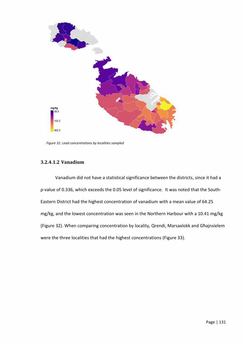
Page | 131
Figure 31: Lead concentrations by localities sampled
3.2.4.1.2 Vanadium
Vanadium did not have a statistical significance between the districts, since it had a
ρ-value of 0.336, which exceeds the 0.05 level of significance. It was noted that the South-
Eastern District had the highest concentration of vanadium with a mean value of 64.25
mg/kg, and the lowest concentration was seen in the Northern Harbour with a 10.41 mg/kg
(Figure 32). When comparing concentration by locality, Qrendi, Marsaxlokk and Għajnsielem
were the three localities that had the highest concentrations (Figure 33).

Page | 132
Figure 32: Vanadium concentrations by district
Figure 33: Vanadium concentrations by localities sampled

Page | 133
3.2.4.1.3 Chromium
The heavy metal chromium resulted to have a ρ-value of 0.450, making it exceed the
0.05 level of significance, and thus the element score between the districts was not
statistically significant. It had an overall average concentration of 22.29 mg/kg. It was found
at a slightly higher concentration in the South-Eastern Harbour at 45.93 mg/kg and a slightly
lower concentration in the district of Gozo and Comino at 8.99 mg/kg (Figure 34) when
comparing with the other districts. When observing the concentration according to the
locality, the most considerable amount found was in Fontana in Gozo, followed by Żejtun,
Għaxaq and Marsaxlokk (Figure 35).
Figure 34: Chromium concentrations by district

Page | 134
Figure 35: Chromium concentrations by localities sampled
3.2.4.1.4 Cadmium
Cadmium was present with an average concentration of 23.51 mg/kg across the
Maltese islands. The metal showed a ρ-value of 0.560; thus, exceeding the 0.05 level of
significance, meaning the element scores vary marginally between the districts. It was found
to be present with the highest concentration in the Northern District at 30.10 mg/kg and
lowest in the Northern Harbour at 16.69 mg/kg (Figure 36). When comparing localities, it
was seen that cadmium was found mostly in Għajnsielem in Gozo, followed by Mġarr,
Għargħur, Qrendi and Siġġiewi (Figure 37).

Page | 135
Figure 36: Cadmium concentrations by district
Figure 37: Cadmium concentrations by localities sampled

Page | 136
3.2.4.1.5 Nickel
This heavy metal had a borderline ρ-value of 0.060. It had a mean concentration of
13.10 mg/kg where it was found in the South-Eastern District with the highest concentration
with a value of 21.90 mg/kg, and was present with the least concentration in the Northern
Harbour District with a value of 2.49 mg/kg (Figure 38). When interpreting the
concentrations found in the localities, Nickel was present at its highest in Għajnsielem,
followed by Qrendi, Marsaxlokk and Bormla (Figure 39).
Figure 38: Nickel concentrations by district

Page | 137
Figure 39: Nickel concentrations by localities sampled
3.2.4.1.6 Cobalt
With a ρ-value of 0.437, cobalt exceeded the 0.05 level of significance stating that
the element score between the districts vary marginally. (Figure 41).

Page | 138
Figure 40: Cobalt concentrations by district
Figure 41: Cobalt concentrations by localities sampled
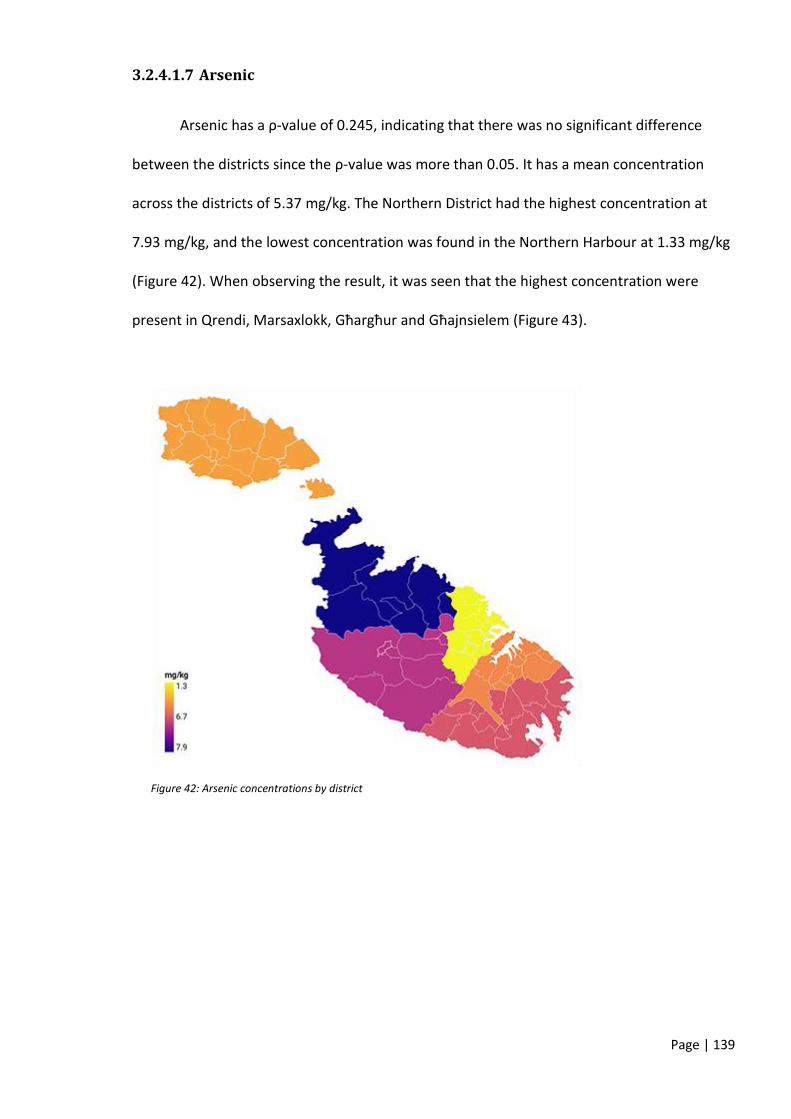
Page | 139
3.2.4.1.7 Arsenic
Arsenic has a ρ-value of 0.245, indicating that there was no significant difference
between the districts since the ρ-value was more than 0.05. It has a mean concentration
across the districts of 5.37 mg/kg. The Northern District had the highest concentration at
7.93 mg/kg, and the lowest concentration was found in the Northern Harbour at 1.33 mg/kg
(Figure 42). When observing the result, it was seen that the highest concentration were
present in Qrendi, Marsaxlokk, Għargħur and Għajnsielem (Figure 43).
Figure 42: Arsenic concentrations by district

Page | 140
Figure 43: Arsenic concentrations by localities sampled
3.2.4.2 P-block elements
The p-block elements consist of silicon, aluminium, bismuth, gallium, germanium,
antimony, selenium, tin and tellurium. The p-block elements are described so as the last
electron moves into one of the three p-orbitals of their corresponding shells (Averill and
Eldredge, 2011c) (Table 14).
Table 14: Mean element value of P-block elements
Element Mean value ppm (mg/kg) Silicon 114070.40
Aluminium 54998.05
Tin 130.07
Antinomy 45.54
Tellurium 44.16
Bismuth 28.97
Selenium 12.31
Gallium 12.01
Germanium 2.36

Page | 141
All the elements in the p-group had ρ-values that exceeded the 0.05 level of significance;
therefore, all the elements were shown to vary marginally. When comparing the p-block
elements, silicon and aluminium had a very high value compared with the rest of the
elements (Figure 44) thus another bar graph was illustrated excluding aluminium and silicon
from the graphs (Figure 45).
Figure 44: P-block element concentrations in each district
Figure 45: P-block concentrations in each district excluding aluminium and silicon

Page | 142
After both silicon and aluminium were removed from the graph, the metals were found
to be as follows in descending order; tin, antimony, tellurium, bismuth, selenium, and
gallium. The element with the least concentration in the group was germanium. Aluminium
was illustrated further using the Datawrapper®.
3.2.4.2.1 Aluminium
The Western District has the highest concentration of aluminium at 38106.00 mg/kg,
while the lowest concentration of aluminium was found in the Northern Harbour at
30414.23 mg/kg (Figure 46). Kerċem had the lowest amount of aluminium from all the
samples with a value of 14713.00 ppm, while Marsaxlokk had the highest values of 54512.75
ppm (Figure 47).

Page | 143
Figure 46: Aluminium concentrations by district
Figure 47: Aluminium concentrations by localities sampled

Page | 144
3.2.4.2.2 Selenium
High concentration of 15.51 mg/kg was seen in both the Northern District and South-
Eastern district when compared to the other districts. The Northern Harbour had the lowest
concentration of Selenium at 9.13 mg/kg (Figure 48). It had an average of 12.31 mg/kg
across Malta and Gozo. Localities having high concentrations were Qrendi, Siġġiewi,
Għargħur, Mġarr, Marsaxlokk, Żurrieq and St. Paul’s Bay (Figure 49).
Figure 48: Selenium concentrations by district

Page | 145
Figure 49: Selenium concentrations by locality
3.2.4.3 S-block elements
The s-block elements are made up of group 1 and 2 in the periodic table. s-block elements
have atoms having their last valence electron, which is present in the s-orbital (Averill and
Eldredge, 2011a).
The mean values of the elements of this group from the One-Way ANOVA show that
sodium is the highest element found in the group, followed by strontium, barium, rubidium
and caesium (Table 15).
Table 15: Mean element values of S-block elements
Element Mean value ppm (mg/kg)
Sodium 96984.42
Strontium 315.32
Barium 185.43
Rubidium 76.39
Caesium 4.30

Page | 146
The bar graph (Figure 50) showed that sodium had a considerable difference in
concentrations compared with the rest of the elements in the group. It was then removed
from the data to draw a bar graph without it (Figure 51). Strontium also proved to have a
high concentration compared to the rest of the elements in the group, while caesium had
the lowest concentration. The Kruskal-Wallis test showed that strontium had a ρ-value of
0.008, which was less than the 0.05 level of significance. Thus the concentrations of the
element was proved to have a statistical difference between the districts.
Figure 50: S-block concentrations in each district

Page | 147
Figure 51: S-block concentrations in each district excluding sodium
3.2.4.4 F-Block elements
Elements in the f-block have atoms with valence electrons in the f-orbital. These are the
inner transition elements from the d-block and are subdivided into two subgroups. If the last
electron moves into the 4f orbital, the elements are placed under the group lanthanides. If
the last electron moves into the 5f orbital, they are placed into the group actinides (Carroll,
2017). The group includes cerium, lanthanum, neodymium and praseodymium (Table 16).
Table 16: Mean element value for F-block elements
Element Mean value ppm (mg/kg)
Lanthanum 29.71
Neodymium 5.24
Cerium 0.74
Praseodymium 0.00
The One-Way ANOVA showed that Lanthanum was found at a higher concentration than
the rest of the elements in this group. All have a ρ-value which exceeded the 0.05 level of
significance showing they did not vary marginally between the districts. The results showed

Page | 148
that the elements in the group were not present in the district of Gozo and Comino. In the
Northern, Western and Northern Harbour District, only lanthanum was seen, although the
Western district had a lesser amount when compared to the other 2 districts. Neodymium
was seen in both South-Eastern and Southern Harbour District, while cerium was only
observed in the Southern Harbour. Praseodymium was not seen in any of the districts
(Figure 52).
Figure 52: F-block concentrations in each district
3.2.5 Localities and districts most affected by the heavy metals
Donut charts using the Datawrapper® were drawn for each heavy metal illustrating were
the element was present at highest concentrations in the localities. Nearly all metals were
seen to be present, mostly in Marsaxlokk and Qrendi. Other common localities between
them are Għajnsielem, Għargħur and Żabbar (Figure 53). Another chart was created to
illustrate the percentage of the element found in the districts (Figure 54).

Page | 149
Figure 53: Elements according to percentage concentration by locality

Page | 150
Figure 54: Percentage concentration of heavy metals by district

Page | 151
Another chart was illustrated using pie charts to depict the percentage difference
between the districts and the highest metal in each district. Aluminium was seen to have the
highest concentration in all of them (Figure 55). Another chart was created, removing
aluminium from the data. Manganese was then shown to have second highest concentration
of the heavy metals in all district, followed by lead, copper and vanadium (Figure 56).
Figure 55: Percentage of heavy metals found in each district

Page | 152
Figure 56: Percentage of heavy metals found in each district excluding aluminium
3.3 Control sample results
The results of the 101 samples taken were compared to the two control samples,
consequently seeing if there were any differences in concentrations between an
uncontaminated soil and the rest of the soil samples which were exposed to fertilizers,
pesticides and other contaminants. The Binomial test was used to compare the mean district
scores with the control values. Nearly all ρ-values, with both controls, were less than the
0.05 level of significance, meaning that the district score, differs significantly from the
control value (Table 17 and Table 18).
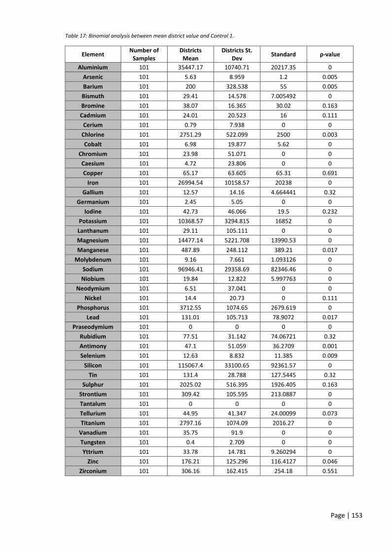
Page | 153
Table 17: Binomial analysis between mean district value and Control 1.
Element Number of
Samples Districts
Mean Districts St.
Dev Standard ρ-value
Aluminium 101 35447.17 10740.71 20217.35 0
Arsenic 101 5.63 8.959 1.2 0.005
Barium 101 200 328.538 55 0.005
Bismuth 101 29.41 14.578 7.005492 0
Bromine 101 38.07 16.365 30.02 0.163
Cadmium 101 24.01 20.523 16 0.111
Cerium 101 0.79 7.938 0 0
Chlorine 101 2751.29 522.099 2500 0.003
Cobalt 101 6.98 19.877 5.62 0
Chromium 101 23.98 51.071 0 0
Caesium 101 4.72 23.806 0 0
Copper 101 65.17 63.605 65.31 0.691
Iron 101 26994.54 10158.57 20238 0
Gallium 101 12.57 14.16 4.664441 0.32
Germanium 101 2.45 5.05 0 0
Iodine 101 42.73 46.066 19.5 0.232
Potassium 101 10368.57 3294.815 16852 0
Lanthanum 101 29.11 105.111 0 0
Magnesium 101 14477.14 5221.708 13990.53 0
Manganese 101 487.89 248.112 389.21 0.017
Molybdenum 101 9.16 7.661 1.093126 0
Sodium 101 96946.41 29358.69 82346.46 0
Niobium 101 19.84 12.822 5.997763 0
Neodymium 101 6.51 37.041 0 0
Nickel 101 14.4 20.73 0 0.111
Phosphorus 101 3712.55 1074.65 2679.619 0
Lead 101 131.01 105.713 78.9072 0.017
Praseodymium 101 0 0 0 0
Rubidium 101 77.51 31.142 74.06721 0.32
Antimony 101 47.1 51.059 36.2709 0.001
Selenium 101 12.63 8.832 11.385 0.009
Silicon 101 115067.4 33100.65 92361.57 0
Tin 101 131.4 28.788 127.5445 0.32
Sulphur 101 2025.02 516.395 1926.405 0.163
Strontium 101 309.42 105.595 213.0887 0
Tantalum 101 0 0 0 0
Tellurium 101 44.95 41.347 24.00099 0.073
Titanium 101 2797.16 1074.09 2016.27 0
Vanadium 101 35.75 91.9 0 0
Tungsten 101 0.4 2.709 0 0
Yttrium 101 33.78 14.781 9.260294 0
Zinc 101 176.21 125.296 116.4127 0.046
Zirconium 101 306.16 162.415 254.18 0.551

Page | 154
Table 18: Binomial analysis between mean district value and Control 2
Element Number of
Samples Districts
Mean Districts St.
Dev Standard ρ-value
Aluminium 101 35447.17 10740.71 23014.35 0
Arsenic 101 5.63 8.959 0.8 0.005
Barium 101 200 328.538 50 0.005
Bismuth 101 29.41 14.578 10 0
Bromine 101 38.07 16.365 32 0.32
Cadmium 101 24.01 20.523 10 0.003
Cerium 101 0.79 7.938 0 0
Chlorine 101 2751.29 522.099 2770 0.551
Cobalt 101 6.98 19.877 5 0
Chromium 101 23.98 51.071 0 0
Caesium 101 4.72 23.806 0 0
Copper 101 65.17 53.605 48.73046 0.32
Iron 101 26994.54 10158.57 23000 0.005
Gallium 101 12.57 14.16 5.01 0.32
Germanium 101 2.45 5.05 0 0
Iodine 101 42.73 46.066 15.31 1
Potassium 101 10368.57 3294.815 12038 0
Lanthanum 101 29.11 105.111 0 0
Magnesium 101 14477.14 5221.708 12013 0
Manganese 101 487.89 248.112 352.64 0
Molybdenum 101 9.16 7.661 1.53 0
Sodium 101 96946.41 29358.69 95824.68 1
Niobium 101 19.84 12.8222 5.62 0
Neodymium 101 6.51 37.041 0 0
Nickel 101 14.4 20.73 0 0.111
Phosphorus 101 3712.55 1074.649 2549.68 0
Lead 101 131.01 105.713 76.1224 0.005
Praseodymium 101 0 0 0 0
Rubidium 101 77.51 31.142 75.0348 0.232
Antimony 101 47.1 51.059 30.246 0.551
Selenium 101 12.63 8.832 10.24 0.046
Silicon 101 115067.4 33100.65 98057.39 0
Tin 101 131.4 28.788 125.876 0.691
Sulphur 101 2025.02 516.395 2000.325 0.842
Strontium 101 309.42 105.595 146.287 0
Tantalum 101 0 0 0 0
Tellurium 101 44.95 41.347 0 0
Titanium 101 2797.16 1074.09 1958.6 0
Vanadium 101 35.75 91.9 0 0
Tungsten 101 0.4 2.709 0 0
Yttrium 101 33.78 14.781 15.021 0
Zinc 101 176.21 125.296 113.2794 0.028
Zirconium 101 306.16 162.415 201.65 0

Page | 155
Chapter 4: Discussion

Page | 156
4.1 Comparison in the pilot study
When comparing the results obtained during the pilot study, it can be observed that the
values between the XRF and the ICP-MS vary. When reading the binomial test, which was
used to evaluate the level of significance, all results showed that the ρ-value exceeded the
0.05 level of significance. Thus, the mean XRF score, is comparable to the ICP-MS value.
The ρ-values obtained were all 1.00 or 0.25, attributing to the fact that for the XRF, only
three readings of each sample where taken. When comparing the results using the
Spearman correlation coefficient, nearly all comparisons proved to have a correlation
coefficient of close to 1, indicating that there was a positive relationship between the results
of the ICP-MS and the XRF. The difference lies in how each instrument works and how they
exhibit their results.
ICP-MS is a very reliable instrument; it is a multipurpose technique that can accomplish
limits of detections many orders of a degree lower than the XRF instrument. It has excellent
accuracy but has the disadvantage that the sample has to be in a liquid form requiring acid
digestion and long sample preparation time when compared to the XRF spectrometer. ICP-
MS cost more to use, including consumables. XRF spectrometer is easier to use and a rapid
technique when comparing it to the other analysis method. It can also read both solid forms
and liquid forms (Al Maliki et al., 2017).
The ICP-MS is a quantitative instrument and has been growing in popularity over
various other instrumentation. It has detection limits which can go below the single part per
trillion of any element, and it can achieve isotopic analysis. The concentration of each
element present in the sample is determined by relating the counts measured of a specific

Page | 157
isotope with an external calibration curve which was previously created for that particular
element (Pröfrock and Prange, 2012; Bulska and Wagner, 2016).
On the contrary, the XRF results are semi-quantitative. Semi-quantitative data
ascertain the relative element concentrations between the samples, but it will not give
absolute concentration amounts. These results are calculated by calculating the area under
the peak of interest, thus showing why the results of both instruments are not identical or
similar, for the elements tested (Bruker, 2020).
4.2 XRF peaks
When reading the XRF spectra, some difficulties may arise when reading them, which
can cause false positive or false negatives, like the chromium and nickel in the results given.
XRF spectra can have peak overlaps which appear due to the presence of individual and
multiple elements in the sample together with limited detector resolution. Peaks seen in the
XRF spectrum can be caused by several sources apart from the metal itself. Artefact peaks
arise due to the X-ray tube source. When the X-ray source photons interact with the
samples, some characteristic features are generated in the XRF spectrum, which may include
Rayleigh peaks, Compton peaks and Bremsstrahlung. Artefact peaks may also be caused by
electrons which have a high kinetic energy of around 10-50 kV, and which strike the atoms in
the X-ray tube source-target which will then transfer energy and cause a peak (Brouwer,
2010; Chemistry LibreTexts, 2019).
Rayleigh Peaks are caused by the elastic scattering from the sample. The elastic
scattering cause peaks on the spectra due to the target anode present in the X-ray tube,
which is made of palladium. During this process, energy is not lost; thus, the peaks show up
at energies which are less than the distinctive X-ray tube target energies. Rayleigh peaks are

Page | 158
usually seen when the samples are dense, and these are observed as weak peaks due to the
amplification of the absorption of palladium’s photons by the sample (Chemistry LibreTexts,
2019).
Compton Peaks are caused by the inelastic scattering from the sample. Once again,
these peaks occur in the spectrum from the palladium element found in the X-ray tube.
During this process, energy is slightly lost; thus, the peaks show up at energies which are
slightly less than the distinctive X-ray tube target energies. Compton peaks are usually seen
when the samples have a low density, and these are observed as fairly intense peaks.
Bremsstrahlung is a backscatter or continuum from a cellulose which is present in all XRF
spectra, where a backscattering of X-rays caused by the sample to the detector causes vast
peaks. It can be seen mostly in less dense samples which tend to scatter more palladium
photons back to the detector. The maximum peak energy limited by kV, which is applied to
the X-ray tube, causes a peak of maximum intensity of around two-thirds of the applied keV.
Other artefact peaks may be caused by the detection process where the X-ray fluorescence
photons interact from the sample with the detector which can generate a variety of artefact
peaks in the spectrum. These artefact peaks are either sum peaks or escape peaks. Sum
peaks are caused by two photons which arrive at the detector at the same time. Sum peaks
are mostly seen when there are high concentrations of an element in the sample. Sum peaks
can be kept on the low side by keeping count rate lows. Escape peaks are caused, by the
absorption of part of the energy of a photon, by silicon atoms present in the detector.
Escape peaks are mostly seen in spectra which have high concentrations of an element
which are lower Z elements. Escape peaks can also be reduced by keeping the count rates
low. Some other artefact peaks may occur from the sampling cup packaging together with

Page | 159
the Mylar film if any contaminants are present on the XRF window (Brouwer, 2010;
Chemistry LibreTexts, 2019).
4.3 Heavy Metals Found in each District and Locality
When seeing the results obtained for each heavy metal and seeing where it was found at
its highest concentration, it can be concluded from where the heavy metal might have
originated. Gozo and Comino District, and the Northern Harbour, where the districts having
the least heavy metal contamination. The districts that had the most pollution of heavy
metals present in their soils, were the South-Eastern District and the Southern Harbour. This
stands to reason since most of the polluting industries are based in these districts.
4.3.1 Aluminium
No limits regarding threshold for aluminium in soil was found. Aluminium was found
nearly in similar amounts all over the Maltese islands. Equal concentrations of aluminium
were observed in the South-Eastern District, Northern District and Western District.
Aluminium is usually present in soils at high concentrations between 10,000 mg/kg and
300,000 mg/kg, since it is the most abundant metal in the Earth’s crust. The average of the
metal present across Malta and Gozo was 34998.05 mg/kg the highest amount observed was
in Marsaxlokk with an average concentration of 54513 mg/kg. Aluminium is identified as a
contaminant of potential concern, but this is only true for those soils that have a pH of less
than 5.5 since it is the only pH where aluminium is present in its soluble form (U.S.
Environmental Protection Agency, 2003; ATSDR, 2008).
4.3.2 Manganese
WHO states that the maximum permissible limit of the heavy metal in medicinal plants is
200 mg/kg (WHO, 2005; Shah et al., 2013). In the United States, the average concentration

Page | 160
of manganese in the soil is between 40-900 mg/kg (ATSDR, 2012c). Though no thresholds are
found to state the maximum limit of manganese in soil. The average concentration of
manganese around the islands was 473.51 mg/kg. It was observed to be present at a higher
concentration in the South-Eastern District and Western District at 586.67 mg/kg and 560.75
mg/kg respectively, when compared to the rest of the districts. Manganese was present
more in these districts probably due to the Delimara power station, smelting of steel
(Rotatori et al., 2003; ERA, 2018) and fertilizers. Qrendi situated in the Western District, had
an average concentration of 887.25 mg/kg, and one particular sample in the locality had a
concentration of 1061 mg/kg. This was where the soil collected from was from land that was
situated close to the area where fireworks had been ignited the week before, and remnants
of the fireworks where still present in the surrounding areas. In Siġġiewi, steel industries are
present which also might be why more manganese was present in the Western District.
4.3.3 Lead
Finland is one of the countries which have soil limits for heavy metals. Finland states that
soil is declared contaminated if one or more of their listed elements is more than the lower
guideline value. The natural concentration of lead in the soil is 5 mg/kg, and the threshold
value is 60 mg/kg. The lower guideline level is stated to be 200 mg/kg, and if the limit is
exceeded health risks are predicted. If the amount is more than the higher guideline level
which is stated to be 750 mg/kg, then it predicted to be of ecological risk (Ministry of the
Environment Finland, 2007). The Dutch limit for lead in soil is stated to be 85 mg/kg, which is
very low compared to the Finland guideline (Ogundele, Adio and Oludele, 2015).
Lead is an element that has brought about much concern about its pollution. It was
observed to have a global average of 125.58 mg/kg. It was present at a very high
concentration of 249.51 mg/kg in the Southern Harbour. The increase in lead in that area

Page | 161
could be due to vehicle emissions, primarily since it used to be added as an anti-knock
vehicle agent (ATSDR, 2019); the shipyard (Papaioannou, 2004; OECD, 2010; Marine Strategy
Framework Directive, 2016) since ships are sandblasted and scraped; use of sewage sludge ;
fuel combustion (Marine Strategy Framework Directive, 2016; Huang et al., 2017; ERA, 2018)
when there was the Marsa power station still working, oil and fuel terminals (Marine
Strategy Framework Directive, 2016), together with the thermal treatment facility (National
Research Council (US) Committee on Health Effects of Waste Incineration, 2000; ERA, 2018)
found in Marsa. All this causes lead particles to spread, and since lead cannot be destroyed,
then it will remain in the soil for long periods and keeps on accumulating.
With regards to localities, it was seen at higher concentrations when compared to the
other localities, in Żabbar, Fgura and Kalkara. Żabbar had an average concentration of 462.33
mg/kg, Fgura was found to have an average concentration of 352.00 mg/kg, and Kalkara had
an average concentration of 301.00 mg/kg. One of the samples of Żabbar had an alarming
concentration of 829.00 mg/kg. Compared to previous studies done in 2006, where Paola’s
topsoil was found to have a lead concentration in its topsoil of 451 mg/kg, Żabbar was seen
to have a very high amount (State of the Environment Indicators, 2006). In various countries,
lead thresholds for residential land is stated with different thresholds according to the
country, as seen in the report by the FAO (Rodriguez-Eugenio, McLaughlin and Pennock,
2018).
Lead concentrations in the district and in the localities with high concentrations all exceed
the Dutch and Finland thresholds. The concentrations even exceed the lower level guideline
making lead toxic in these areas.

Page | 162
4.3.4 Copper
The Dutch permissible limit for copper in the soil is 36 mg/kg (Ogundele, Adio and
Oludele, 2015). The Finland law states that the natural concentration of copper is 22 mg/kg,
and the threshold value is 100 mg/kg. The lower guideline value, which can be of ecological
risk is 150 mg/kg (Ministry of the Environment Finland, 2007). Quite a lot of localities had
more than the lower guideline value of the Finland soil contamination law, and only a few
localities had less than the 36 mg/kg as stated in the Dutch permissible limit law (Ogundele,
Adio and Oludele, 2015). The FAO states a variety of copper limits for residential land
depending on the country (Rodriguez-Eugenio, McLaughlin and Pennock, 2018).
The highest concentration of copper was noted in the Southern Harbour area, with an
average concentration of 95.15 mg/kg. Increase in copper concentrations observed in the
Southern Harbour District could be due to the shipyard’s activity (Papaioannou, 2004; OECD,
2010; Marine Strategy Framework Directive, 2016) and the previous power station (Marine
Strategy Framework Directive, 2016; Huang et al., 2017). Other methods of copper pollution
could be due to the use of fungicidal in plants which is sometimes added in excess in the
agricultural land due to pig and cow manure (Xiong et al., 2010; Jiang, Dong and Zhao, 2011),
and the use of sewage sledge (Marine Strategy Framework Directive, 2016; US EPA, 2019a).
It was found at higher concentration in the localities of Qrendi and Għargħur soil samples at
128.75 mg/kg and 137 mg/kg respectively, due to the fireworks activities since copper is one
of the elements used to project the blue colour. Bormla at 136 mg/kg, Fgura at 120.50
mg/kg and Żabbar at 124.67 mg/kg, have high concentrations since they are situated in the
Southern Harbour. St. Julians had the highest concentration of 140 mg/kg, though the source
of pollution was not discovered.

Page | 163
Most values exceed the Dutch threshold and the copper concentrations found in the
localities with the highest concentrations exceed Finland’s threshold value.
4.3.5 Vanadium
According to Finland’s permissible limits, the natural occurrence of vanadium is 38 mg/kg,
the threshold value is 100 mg/kg, and the lower and higher guideline values are 150 mg/kg
and 250 mg/kg respectively (Ministry of the Environment Finland, 2007). Vanadium had an
average concentration of 32.75 mg/kg. The South-Eastern District had the highest
concentration of vanadium present when compared to the rest of the districts with an
average of 64.25 mg/kg. Fly ash from power stations is one of the reasons for vanadium to
be present in the soil after settling or washed from the atmosphere (ATSDR, 2012d).
Qrendi and Marsaxlokk had very high concentrations of vanadium of 244.75mg/kg and
244 mg/kg respectively, where in one of the Qrendi samples, vanadium was present at a
concentration of 683 mg/kg. When seeing localities and individual samples. Qrendi might
have resulted in a high concentration of vanadium due to the fireworks since both
aluminium and vanadium elements can be found in titanium powders which are used for
fireworks (ATSDR, 2012d; Ogundele, Adio and Oludele, 2015).. When seeing the
concentrations by districts, vanadium concentrations are within range, though when
comparing the individual samples, the Qrendi and Marsaxlokk samples were in excess and
over the thresholds.
4.3.6 Cadmium
According to the Finland law, the natural concentration of cadmium is 0.03 mg/kg, and
the threshold value is 1 mg/kg. The law also states that the lower guideline limit and the
upper guideline limits are 10 mg/kg and 20 mg/kg, respectively (Ministry of the Environment

Page | 164
Finland, 2007). The permissible limit by the Dutch standard is 0.8 mg/kg (Ogundele, Adio and
Oludele, 2015). Cadmium had an average concentration of 23.51 mg/kg around Malta and
Gozo. The district with the highest cadmium present was in the Northern district at 30.10
mg/kg. This might be due to the Magħtab landfill, which in the past, batteries were part of
the waste delivered and no capping was present. Batteries contain cadmium and could have
leached out of the landfill (Panero et al., 1995). It was also found at high concentrations in
the South-Eastern District at 28.95 mg/kg which might have been caused by the Delimara
power station (Rotatori et al., 2003; Marine Strategy Framework Directive, 2016; Huang et
al., 2017) or the use of sewage sludge (Marine Strategy Framework Directive, 2016; US EPA,
2019a). It was found in Għajnsielem and Ta’ Sannat in Gozo as the localities that contained
cadmium at high concentrations which might come from phosphate fertilizers (Cupit et al.,
2002) or from the cement plant located in the locality which is a source of cadmium
pollution (ERA, 2018; US EPA, 2019b) or from the sewage plant situated in Għajnsielem, Ras
il-Ħobż (Lindqvist-Östblom and Eklund, 1999) .
Cadmium is found at very high concentrations when compared to the Dutch standard
and Finland standard which exceed the upper level guideline (Ministry of the Environment
Finland, 2007; Ogundele, Adio and Oludele, 2015).
4.3.7 Chromium
According to the Dutch standard, the limit of permissible chromium is 100 mg/kg
(Ogundele, Adio and Oludele, 2015). The Finland standard states that the natural
concentration of chromium is 31 mg/kg, and the threshold value should be 100 mg/kg.
When seeing the lower guideline value, this is stated as 200 mg/kg and the higher guideline
value is stated to be 300 mg/kg to be of ecological risk (Ministry of the Environment Finland,
2007). The average concentration of chromium is 22.29 mg/kg and was found to be highest

Page | 165
in the South-Eastern District with an average concentration of 45.93 mg/kg. Chromium
might be released into the atmosphere through the Delimara power stations (Rotatori et al.,
2003; Marine Strategy Framework Directive, 2016) and oil and fuel terminals (Marine
Strategy Framework Directive, 2016). Chromium in this research was not detected to see
which oxidation was present, whether it was chromium (III) or chromium (VI). The oxidation
makes all the difference when it comes to chromium toxicity. Chromium might be released
into the atmosphere through the Delimara power stations (Rotatori et al., 2003; Marine
Strategy Framework Directive, 2016).
Some localities had an amount of more than 100 mg/kg of chromium and thus were more
than the permissible limit compared to both Finland and the Dutch thresholds.
4.3.8 Arsenic
The Finland standard states that the natural concentration of arsenic is 1 mg/kg and the
threshold concentration is 5 mg/kg. Lower and higher guideline values are 50 mg/kg and 100
mg/kg which will cause risk to the ecology (Ministry of the Environment Finland, 2007). One
of the toxic elements is arsenic which was found in the Northern district at higher
concentrations when compared to the other districts at 7.93 mg/kg. The high amount of
arsenic in the Northern District after talking to the farmers could be as poultry and pig
manure was used in their soils which might have contained arsenic.
With regards to localities, arsenic was found mostly in Qrendi, with an average
concentration of 23.75 mg/kg, Għargħur, with an average concentration of 22 mg/kg, and
Marsaxlokk, with an average concentration of 22mg/kg. In the past arsenic was used in
fireworks to give more colour. Since it is toxic, it has been reduced or not used at all, though
it was seen at high amounts in both places were soil samples were taken just after the

Page | 166
fireworks were displayed, thus fireworks might be the cause of the increase of arsenic in
these samples. Sewage sludge also may contain arsenic in it (US EPA, 2019a) and if farmers
used it untreated, this could be the cause for an increase in the metal presence. In the
locality of Marsaxlokk, the amount of arsenic observed could be due to the release from the
power station since arsenic is detected in electricity generation plants (Rotatori et al., 2003;
ERA, 2018) or through the wear of tyres and breaks (ERA, 2018). It was used as a rat poison
in previous times and still might linger in the soil since it is not biodegradable (Brown and
Waddell, 2014). Arsenic in Qrendi was found to be at 23.75 mg/kg which is alarmingly high
for an element so toxic when compared to the threshold value stated by Finland
4.3.9 Cobalt
The threshold value from the Finland standard is 20 mg/kg. The lower and upper
guideline values are stated as 100 mg/kg and 250 mg/kg (Ministry of the Environment
Finland, 2007). Cobalt can be seen at 15.83 mg/kg in the district of Gozo and Comino, which
has the highest average concentration of the metal present. Cobalt can be present in
fertilizers, sewage sludge and animal feed (Cobalt Institute, 2017; US EPA, 2019a). Kirkop
was one of the localities with the highest average concentration of cobalt at 63.50 mg/kg.
This increase in cobalt in this area could be due to airport traffic which releases cobalt into
the air (ATSDR, 2004b).
As an average concentration and district, cobalt is observed to be below the threshold
stated by Finland. When looking at some individual localities such as Ħal-Safi, the
concentration exceeds the threshold stated.

Page | 167
4.3.10 Nickel
The Dutch standard states that the permissible limit for nickel should be 35 mg/kg
(Ogundele, Adio and Oludele, 2015). According to the Finland standard, the threshold
concentration of nickel should be 50 mg/kg and the lower and higher guideline values are
100 mg/kg and 150 mg/kg respectively (Ministry of the Environment Finland, 2007). An
average concentration of 13.10 mg/kg of nickel was observed around Malta and Gozo. The
heavy metal nickel was found to be present at a high concentration in the South-Eastern
District and the South Harbour. It was present at 21.90 mg/kg and 19.95 mg/kg respectively.
These districts might have showed a higher concentration due to the shipyards
(Papaioannou, 2004; OECD, 2010), the Delimara power station (Rotatori et al., 2003; ERA,
2018), waste incineration (ERA, 2018), oil and fuel terminals (Marine Strategy Framework
Directive, 2016) and the combustion of fuel in ships (ERA, 2018).The localities which had the
highest concentration of this element was Għajnsielem, with an average of 61 mg/kg
probably due to the sewer plant , and Marsaxlokk had an average of 55 mg/kg probably due
to the Delimara power station (Marine Strategy Framework Directive, 2016). Qrendi had one
of its samples show a concentration of 63 mg/kg, which might have been caused by the
ignition of fireworks (Helmenstine, 2020), and Bormla had one sample showing an amount
of 79 mg/kg of nickel, probably due to shipyards (Papaioannou, 2004; OECD, 2010).
On seeing the values of the soil samples collected, on average, the amount of nickel
present is less than both the Dutch and the Finland standard. Some agricultural lands have
more than the permissible limit.

Page | 168
4.3.11 Molybdenum
No threshold limits were found on this metal. It was found with an average of 8.85 mg/kg
around Malta and Gozo. It was found at higher concentration in the Northern District with
an average of 12.09 mg/kg. This could be due to the wastewater treatment plant and the
landfill situated in this district (ATSDR, 2004b). When observing localities, the highest
concentration was found in Għajnsielem with an average concentration of 23.00 mg/kg
which could be due to the sewage plant there (ATSDR, 2004b). It was followed by Qrendi and
Għargħur with average concentrations of 21.00 mg/kg for the both of them. This could be
due to the fireworks as molybdenum can be carbonised to suppress smoke in the fireworks
(Stanford Advanced Materials, 2017). It was found with an average concentration of 20.00
mg/kg in Marsaxlokk showing that the pollution may have been caused by the Delimara
power station (ATSDR, 2004b).
4.3.12 Selenium
No threshold limits for selenium present in soil, were found. It was present with an
average concentration of 12.31 mg/kg and although it was found at similar concentrations
all over the islands, it had a slightly higher in the South-Eastern District with an average of
15.50 mg/kg probably due to the Delimara power station, since selenium is one of the
pollutants caused by energy generation industries (Staicu et al., 2017). On seeing localities,
the sample in Għargħur showed selenium to be present at 28 mg/kg.
4.3.13 Zinc
The natural concentration and threshold value of zinc, according to the Finland
legislation, are 31 mg/kg and 200mg/kg. The lower guideline value is stated as 250 mg/kg
and the upper guideline value is stated as 400 mg/kg (Ministry of the Environment Finland,

Page | 169
2007). The maximum limit by the Dutch standard is 50mg/kg (Ogundele, Adio and Oludele,
2015)(Ogundele <i>et al.</i>, 2017). The average concentration across the islands was at
174.09 mg/kg. It was found with a very high concentration in the Southern Harbour at
251.33 mg/kg when compared to the other districts. This high concentration may be due to
the shipyard activities (Papaioannou, 2004; Marine Strategy Framework Directive, 2016),
sewage sludge, oil and fuel terminals, and the old Marsa power station (Marine Strategy
Framework Directive, 2016).
The localities with the most zinc present in their soil were in the locality of Żabbar which
was found with a concentration of 447.20 mg/kg. Following Żabbar, zinc was found at high
concentrations in Bormla at 376.80 mg/kg, Mġarr at 350.80 mg/kg and Għajnsielem at
326.20 mg/kg. Żabbar and Bormla may had high concentrations due to the shipyard, old
Marsa power station and oil and fuel terminals. Mġarr may had high concentrations due to
the addition of poultry and pig manure (Jiang, Dong and Zhao, 2011), since this was
confirmed by the farmer. Ghajnsielem’s zinc increase may be due to the sewage plant or the
cement plant (ERA, 2018; US EPA, 2019b).
4.4 Controls
In both Binomial tests, H1 was not rejected since the sample mean of the 101
observations vary significantly from the control one values and control two values. The
heavy metals in both controls were significantly lower than the rest of the samples. Copper
in control one is not significantly different as the ρ-value exceed the 0.05 level of significance
since the element was confirmed to be used by the farmer as a fungicide, increasing the
amount of copper in the soil. Concentration of chlorine in control two, was observed to be
higher than control one values, and this may have been brought about by strong winds

Page | 170
which carries sea droplet onto the soil due to the close proximity of the agricultural land to
the sea.
4.5 Limitations and Recommendations for Future Work
When preparing the soil, the sampling cup technique was used for this research study.
One of the disadvantages is that the soil had to be fine, no air pockets, moisture or organic
matter had to be present. If any of these were present the R/R0 would increase, the fit would
not be good, and thus results will be even less accurate. For better analytical results, another
sampling technique could have been used, which is the pressed pellet technique. Pellets
have a higher signal to noise ratio than when testing the loose powder form. The lightest
elements in the sample are detected, and the lighter elements are also detected without
being underestimated. Unlike loose powder, where lighter elements might go undetected.
When arranging the loose soil in the sample cup, pockets of air can also affect the reading
and thus from one sample to the next, the reading may vary depending on how homogenous
the sample was and how compact it was prepared. The advantage of loose powder is an
effortless preparation. Pressed pellets, on the contrary, need more preparation. The process
of pressed pellets involves the sample being ground to very fine particle size. This fine
particle soil sample is then mixed with a binder in a grinder or mixing vessel. The mixture
achieved is then poured into a pressing die where the mixture is pressed at a pressure
between 15T and 35T. Contamination is one of the aspects that needs to be seen when
preparing it. Some details should be done with care when using the pressed pellet, such as
the particle size, binder choice, ratio of dilution, amount of pressure used to form the pellet
and the thickness of the pellet, to get high-quality results (Coler, 2017).

Page | 171
Another limitation for these results is that each sample was only tested three times to get
a global picture of the result. For better correlation values, more readings could have been
done, where each sample could have been repeated at least 15 times to get a more accurate
analysis.
When comparing the ICP-MS and the XRF, it could be seen that elements present in low
amounts, such as mercury which is a very toxic heavy metal, was not seen in the XRF results.
Some elements such as chromium and nickel were present in the sample but were not
calculated by the XRF programme. This was due to the R/R0 fitting which sometimes
eliminated these elements, even though the peak was present. XRF oxidation states of
elements was another issue while using the XRF as the oxidation state could not be
identified, changing the scenario for some heavy metals where one oxidation state can be
toxic and other not. Case in point is chromium, which can be present as chromium (III) or
chromium (VI) which have very different properties and toxicity properties. Chromium (VI) is
very toxic, while chromium (III) is not.
An important parameter which can be taken into account to get a better picture of
toxicity is the soil’s pH. The difference in soil pH, as previously explained, can cause the
element to be absorbed or not absorbed by the plant. Thus, pH will decide if the heavy
metal will be toxic to the plant and thus toxic to the rest of the food chain. In most heavy
metals, the more acidic the soil is, the more the heavy metal will be absorbed, and thus the
more toxic the element becomes. Other parameters include the oxidation state, the organic
matter, and redox reactions. The type of plant grown in the soil and plant pattern can also
be another factor which causes a difference in the absorbance of the heavy metal.
Dicotyledons tend to absorb heavy metals more than monocotyledons.

Page | 172
Another area that could be looked into are soil from glasshouses. The soil in these
glasshouses are not contaminated by air pollutants, since no dissolved contaminants can
reach the soil. The soil in the glasshouses could have shown that plants grown in the
enclosed area would contain fewer contaminants than plants grown outside.
4.5.1 Practices to Target High Levels of Heavy Metal Concentrations
A lot of technologies or treatments are present to try and remove the heavy metals from
the contaminated soils. Some techniques can be done on-site, while other techniques need
the soil to be removed and treated off-site.
Remediation techniques can be divided into three types; (i) physical, (ii) chemical, (iii)
biological. Physical remediation techniques include methods such as thermal, solidification,
vapour extraction, washing and treating, air sparging, particle sorting, and electromediation.
Chemical remediation methods include oxidation, hydrolysis, reduction, solubilisation, pH
manipulation and dechlorination. The third type of method is uses the biological techniques
which include landfarming, microbial activity, bioreactor, composting, bioleaching,
phytostabilisation, plant activity, phytoextraction and photodegradation (Rodriguez-Eugenio,
McLaughlin and Pennock, 2018).
Some of the methods might be too expensive or time-consuming. Massive volumetric
sludge is generated when using the chemical technologies and these also increase the costs.
Thermal methods, apart from being expensive to perform, can also damage essential soil
components. Traditionally, onsite management of heavy metal contaminated soil
remediation occurred, or excavation of the contaminated soil which was disposed to a
landfill. Though this has proven to being just a transportation of the contaminated soil, to a
different location instead of reducing or eliminating the contamination, this method

Page | 173
increases the chance to contaminate other areas next to the landfills. An alternative method
that is used is soil washing. This method can be used instead of the excavation method, and
involves washing the soil to remove the metals. However, it is costly, and the residue
produced is highly abundant in the metals that were eliminated, and would thus need
further treatment. From all these methods, it can be observed that soil remediation using
physio-chemical technologies tends to eradicate all the biological activities, and thus reduces
the medium for the plant growth (Wuana and Okieimen, 2011). Phytoremediation and
intercrop are newer techniques which are widely being used.
4.5.2 Phytoremediation
Phytoremediation has become a more popular method since it is less expensive and
environmentally friendly. Plants are planted in soils that are contaminated with heavy
metals to aid in the removal. Apart from removing heavy metals from soils,
phytoremediation has also been used to remove heavy metals from sediment and waters.
These type of plants are known as hyperaccumulator plants (Hao et al., 2012).
Plant root systems are selective in their uptake and thus prove to be an advantage in
phytoremediation. This also includes translocation of the contaminant, bioaccumulation and
the degradation of the entire plant to remove the heavy metal. Inorganic compounds
removal involved in this process usually takes place through phytostabilisation and
phytoextraction. Phytoextraction involves the heavy metal being translocated from the
roots into the shoots. In contrast, phytostabilisation involves certain plant species which
absorb and accumulate the heavy metals in certain parts of the plants and thus stop the
movement of the element from going back into the soil. The removal of organic compounds
is usually achieved through phytodegradation, rhizodegradation and rhizofiltration.
Rhizodegradation needs microbial activity to degrade the contaminants in the rhizosphere,

Page | 174
which is improved by the plant roots. Rhizofiltration consists of the precipitation or the
adsorption of the contaminants into the roots that are in the solution surrounding the root
by wetting the land (Tangahu et al., 2011).
Certain factors which influence the uptake of the metal is the plant species; the
properties of the medium include, the pH of the soil, the organic matter present and the
phosphorous amount present together with other factors; the root zone; vegetative uptake
which is affected by the temperature since it affects the root length; and the chelating agent
added which influences the bioavailability of the heavy metals. Some examples of a chelating
agent used are ethylenediaminetetraacetic acid EDTA (Chen, Li and Shen, 2004; Tangahu et
al., 2011; Wuana and Okieimen, 2011).
The Chinese Brake plant known as Pteris vittata L. absorbs around 0.7 mg/g or more of
arsenic in the dry weight in the whole plant. The black poplar, known as Populus nigra
absorbs around 0.2 mg/g arsenic per dry weight in its roots. Lead is absorbed by the plant
Brassica carinata A. Braun also known as Abyssinian cabbage or Abyssinian mustard, which
absorbs lead at more than 50 mg/g of dry plant weight. Tomato plants, Solanum
lycopersicum, absorb cadmium in its shoots and lead in its roots. The tomato itself is also a
part of the plant that absorbs excess cadmium. Thlaspi caerulescens is a hyperaccumulator
for zinc and cadmium. It can take up to 10,000 mg/kg of zinc and cadmium is taken up by the
shoots with an amount of 100 mg/kg of dry plant weight. The plants do not show signs of
toxicity when taking up the heavy metals (An et al., 2011a).
4.5.3 Intercropping
Intercropping involves the simultaneous growth of two plants or more. Intercropping
helps twofold to improve the plant biomass, and in aiding with the accumulation of heavy

Page | 175
metals. Phytoremediation can be further improved by intercropping with another plant
species to help increase heavy metal absorption. This combination of methods will help to
be more environmentally friendly, unlike the use of chelators (Li et al., 2009; Cui et al.,
2018). For a successful intercropping system to happen, the appropriate component species
or population needs to be selected. Apart from decreasing the heavy metals, intercropping
helps in increasing income for the farmers (Wan and Lei, 2018).
Due to the intercropping method, some benefits that are acquired include stability and
diversity brought to the fields, fertilizer application reduction and crops used together to
share resources. Lastly, there can be a reduction of weeds, insects or disease acquirement
(Lowry and Smith, 2018). Three types of intercropping exist, (i) mixed intercropping - when
the different crops are harvested together; (ii) row intercropping - the method used when
the different crops are grown in alternative rows; and (iii) relay cropping – when the
reproductive stage of the first crop is waited for until the second crop can be sown
(Lithourgidis et al., 2011).
Examples of intercropping plants used and the heavy metal affected by the method are,
maize and chickpea plants. Maize absorbs a decent amount of cadmium from the soil, but
when it is intercropped with chickpea, the amount is increased (Li et al., 2009). Another
example is tomato intercropped with the Japan clover herb. Iron concentration increases in
the tomato root when it is harvested with the Japan clover herb. Also with this
intercropping, cadmium was found at higher quantities in is shoots, roots and fruit. Japan
clover herb had high values of cadmium when intercropped with both the tomato plant and
the maize plant (An et al., 2011b).

Page | 176
4.5.4 Organic Farming
There are several organic farms registered in Malta, were no artificial pesticides and
synthetic fertilizers are used to control their plants. Increased use of pesticides and fertilizer
has reduced the biodiversity around the lands in Malta since it is not only toxic to the pests,
but also to the other insects and reptiles. Such as the Coccinellidae which is known as the
ladybird, Lumbricus spp. known as the earthworm, Apis mellifera ruttneri which is the
Maltese honey bee.
On the contrary, organic farming uses the biodiversity to their advantage. Many insects
and reptiles have habitats in the area which roam the lands and remove any unwanted pests
themselves. Unlike other farmers who make use of chemicals to remove the pests. Since
habitats and food is increased, wild fauna and flora increase in the area, including pest
predators and pollinators. According to the organic farmers that were talked to during the
research, examples of natural pest predators are spiders which emerge during the night
removing quite a lot of pest insects from the crops. Chameleons are insectivores and help in
the removal of insects such as whiteflies and red spiders, which can destroy the crops.
Butterflies and honey bees are found in higher quantities which help in pollination. Ladybirds
are found in large quantities which are known to kill aphids which remove the sap from the
plant (FAO, 2020).
Apart from organic farms benefiting the microbial activity and also the biodiversity in
Malta, it also uses no chemicals and is thus pollution-free. Since figures show that the heavy
metals were low in the organic farms, it can be deduced that the crops grown in these farms
will not cause any toxic effects to animals or humans since less amount were found in the
soil, for them to be absorbed.

Page | 177
4.6 Conclusion
Heavy metal pollution has been given a lot of attention since heavy metals is a source of
toxicity. They are not biodegradable and remain in the soil indefinitely. The bioaccumulation
of heavy metals in soil can be the cause of detriment to plants, animals and humans as the
metals can be absorbed by the plants, and end up in the food chain, which may produce
adverse effects including death.
This study has shown how heavy metal pollution in Maltese soils, may have been brought
about. Sources of heavy metal pollution, have been noted to be more abundant in areas
where there is industrialisation which has been observed as heavy metals was observed in
the South-Eastern and South Harbour Districts. Lead, arsenic, cadmium and zinc were some
of the heavy metals which were found to surpass thresholds according to the Finland and
Dutch legislation. Methods to address excess heavy metals in soils can be applied to reduce
the metals such as remediation and intercropping. The study revealed that organic farming is
a way of growing crops without the use of pesticides and artificial fertilizers, which has
shown that soils in organic farms, have a less concentration of each of the heavy metals
discussed.

Chapter 5: Bibliography
Page | 179
Adrees, M. et al. (2015) ‘The effect of excess copper on growth and physiology of important food crops: a review’, Environmental Science and Pollution Research. Springer Verlag, 22(11), pp. 8148–8162. doi: 10.1007/s11356-015-4496-5.
Agrafioti, E., Kalderis, D. and Diamadopoulos, E. (2014) ‘Arsenic and chromium removal from water using biochars derived from rice husk, organic solid wastes and sewage sludge’, Journal of Environmental Management. Academic Press, 133, pp. 309–314. doi: 10.1016/j.jenvman.2013.12.007.
Aihemaiti, A. et al. (2019) ‘Review of plant-vanadium physiological interactions, bioaccumulation, and bioremediation of vanadium-contaminated sites’, Science of the Total Environment. Elsevier B.V., p. 135637. doi: 10.1016/j.scitotenv.2019.135637.
Aktar, W., Sengupta, D. and Chowdhury, A. (2009) ‘Impact of pesticides use in agriculture: Their benefits and hazards’, Interdisciplinary Toxicology, 2(1), pp. 1–12. doi: 10.2478/v10102-009-0001-7.
Albanese, S. et al. (2007) ‘Geochemical background and baseline values of toxic elements in stream sediments of Campania region (Italy)’, Journal of Geochemical Exploration, 93(1), pp. 21–34. doi: 10.1016/j.gexplo.2006.07.006.
Alloway, B. J. and Jackson, A. P. (1991) ‘The behaviour of heavy metals in sewage sludge-amended soils’, Science of the Total Environment, The, 100(C), pp. 151–176. doi: 10.1016/0048-9697(91)90377-Q.
An, L. et al. (2011a) ‘Heavy metal absorption status of five plant species in monoculture and intercropping’, Plant and Soil, 345(1), pp. 237–245. doi: 10.1007/s11104-011-0775-1.
An, L. et al. (2011b) ‘Heavy metal absorption status of five plant species in monoculture and intercropping’, Plant and Soil, 345(1), pp. 237–245. doi: 10.1007/s11104-011-0775-1.
Aronsson, P. and Perttu, K. (2001) ‘Willow vegetation filters for wastewater treatment and soil remediation combined with biomass production’, Forestry Chronicle. Canadian Institute of Forestry, 77(2), pp. 293–299. doi: 10.5558/tfc77293-2.
Ashraf, M. A. (2017) ‘Persistent organic pollutants (POPs): a global issue, a global challenge’, Environmental Science and Pollution Research. Springer Verlag, pp. 4223–4227. doi: 10.1007/s11356-015-5225-9.
ATSDR (1999) Toxicological Profile for Mercury. Available at: https://www.atsdr.cdc.gov/toxprofiles/tp46.pdf (Accessed: 29 June 2018).
ATSDR (2003) Toxicological Profile for Selenium. Available at: https://www.atsdr.cdc.gov/ToxProfiles/tp92.pdf (Accessed: 29 June 2018).
ATSDR (2004a) Toxicological Profile for Copper. Available at: https://www.atsdr.cdc.gov/toxprofiles/tp132.pdf (Accessed: 29 June 2018).
ATSDR (2004b) Toxicological Profile of Cobalt. Available at: https://www.atsdr.cdc.gov/ToxProfiles/tp33-c1-b.pdf.
ATSDR (2005) Toxicological Profile for Zinc. Available at: https://www.atsdr.cdc.gov/ToxProfiles/tp60.pdf.
ATSDR (2007a) Toxicological Profile for Arsenic. Available at: https://www.atsdr.cdc.gov/toxprofiles/tp2.pdf (Accessed: 29 June 2018).
ATSDR (2007b) Toxicological Profile for Lead. Available at: https://www.atsdr.cdc.gov/toxprofiles/tp13.pdf (Accessed: 29 June 2018).
ATSDR (2008) Toxicological Profile for Aluminium. Available at:

Page | 180
https://www.atsdr.cdc.gov/toxprofiles/tp22.pdf.
ATSDR (2012a) Toxicological Profile for Cadmium. Georgia. Available at: https://www.atsdr.cdc.gov/toxprofiles/tp.asp?id=48&tid=15 (Accessed: 29 June 2018).
ATSDR (2012b) Toxicological Profile for Chromium. Available at: https://www.atsdr.cdc.gov/csem/chromium/docs/chromium.pdf (Accessed: 29 June 2018).
ATSDR (2012c) Toxicological Profile for Manganese.
ATSDR (2012d) Toxicological Profile for Vanadium. Available at: https://www.atsdr.cdc.gov/toxprofiles/tp58.pdf (Accessed: 25 June 2018).
ATSDR (2017) Toxicological Profile for Nickel. Available at: https://www.atsdr.cdc.gov/ToxProfiles/tp15-c1-b.pdf (Accessed: 29 June 2018).
ATSDR (2019) Toxicological Profile for Lead.
Averill, B. A. and Eldredge, P. (2011a) ‘Periodic Trends and the s-Block Elements’, in General Chemistry: Principles, Patterns, and Applications. Saylor Foundation.
Averill, B. A. and Eldredge, P. (2011b) ‘The d-Block Elements’, in General Chemistry: Principles, Patterns, and Applications. Saylor Foundation. Available at: https://2012books.lardbucket.org/books/principles-of-general-chemistry-v1.0m/s27-the-d-block-elements.html (Accessed: 5 March 2020).
Averill, B. A. and Eldredge, P. (2011c) ‘The p-Block Elements’, in General Chemistry: Principles, Patterns, and Applications. Saylor Foundation.
Axiak, P. V. (2004) Assessing the marine environmental quality of the coastal waters exposed to the Maghtab Solid Waste Disposal Site FINAL REPORT ENVIRONMENT PROTECTION DIRECTORATE Malta Environment and Planning Authority.
Baderna, D. et al. (2011) ‘A combined approach to investigate the toxicity of an industrial landfill’s leachate: Chemical analyses, risk assessment and in vitro assays’, Environmental Research, 111(4), pp. 603–613. doi: 10.1016/j.envres.2011.01.015.
Baishya, K. (2015) ‘Impact of Agrochemicals Application on Soil Quality Degradation - A Review’, International Journal of Science Technology and Management, 4(1).
Balkhair, K. S. (2016) ‘Microbial contamination of vegetable crop and soil profile in arid regions under controlled application of domestic wastewater’, Saudi Journal of Biological Sciences, 23(1), pp. 83–92. doi: Balkhair, K. S. (2016). Microbial contamination of vegetable crop and soil profile in arid regions under controlled application of domestic wastewater. Saudi Journal of Biological Sciences, 23(1), S83–S92. doi:10.1016/j.sjbs.2015.10.029.
Barceló, D. and Petrovic, M. (2007) ‘Pharmaceuticals and personal care products (PPCPs) in the environment’, Analytical and Bioanalytical Chemistry, pp. 1141–1142. doi: 10.1007/s00216-006-1012-2.
Barnes, J. (2009) Assessment of Air Quality in the Vicinity of Delimara Power Station, Malta Baseline.
Barnhart, J. (1997) ‘Occurrences, Uses, and Properties of Chromium’, Regulatory Toxicology and Pharmacology. Academic Press Inc., 26(1 I), pp. S3–S7. doi: 10.1006/rtph.1997.1132.
Basile, B. P., Middleditch, B. S. and Oró, J. (1984) ‘Polycyclic aromatic hydrocarbons in the Murchison meteorite’, Organic Geochemistry, 5(4), pp. 211–216. doi: 10.1016/0146-6380(84)90008-1.
Battist, L. and Peterson, H. T. (1980) ‘Radiological Consequences of the Three Mile Island Accident’, in Radiation Protection. Oxford: Pergamon Press, pp. 677–684.

Page | 181
Bayat, J. et al. (2016) ‘Fingerprinting aliphatic hydrocarbon pollutants over agricultural lands surrounding Tehran oil refinery’, Environmental Monitoring and Assessment. Springer International Publishing, 188(11). doi: 10.1007/s10661-016-5614-7.
Beasley, M. and Temple, W. (no date) ‘Pyrethroid toxicity and its management’, Best Practice Journal - Hazardous Substances Series.
Benavides, M. P., Gallego, S. M. and Tomaro, M. L. (2005) ‘Cadmium toxicity in plants’, Brazilian Journal of Plant Physiology. Sociedade Brasileira de Fisiologia Vegetal, pp. 21–34. doi: 10.1590/S1677-04202005000100003.
Bengtsson, B. et al. (1988) ‘Influence of aluminium on phosphate and calcium uptake in beech (Fagus sylvatica) grown in nutrient solution and soil solution’, Physiologia Plantarum, 74(2), pp. 299–305. doi: 10.1111/j.1399-3054.1988.tb00635.x.
Bhalerao, S. A., Sharma, A. S. and Poojari, A. C. (2015) ‘Toxicity of Nickel in Plants’, Interrnational Journal of Pure and Applied Bioscience, 3(2), pp. 345–355.
Birch, G. F. and Scollen, A. (2003) ‘Heavy metals in road dust, gully pots and parkland soils in a highly urbanised sub-catchment of Port Jackson, Australia’, Australian Journal of Soil Research, 41(7), pp. 1329–1342. doi: 10.1071/SR02147.
Blaser, P. et al. (2000) ‘Critical examination of trace element enrichments and depletions in soils: As, Cr, Cu, Ni, Pb, and Zn in Swiss forest soils’, Science of the Total Environment, 249(1–3), pp. 257–280. doi: 10.1016/S0048-9697(99)00522-7.
Bogden, J. D. and Louria, D. B. (1975) ‘Soil contamination from lead in paint chips’, Bulletin of Environmental Contamination and Toxicology. Springer-Verlag, 14(3), pp. 289–294. doi: 10.1007/BF01685637.
Bolívar, J. P., García-Tenorio, R. and García-León, M. (1995) ‘Enhancement of natural radioactivity in soils and salt-marshes surrounding a non-nuclear industrial complex’, Science of the Total Environment, 173–174(C), pp. 125–136. doi: 10.1016/0048-9697(95)04735-2.
Brady, N. C. (1990) The Nature and Properties of Soils, Macmillan Publishing Company. Available at: https://www.nrcs.usda.gov/wps/portal/nrcs/detail/nj/home/?cid=nrcs141p2_018993 (Accessed: 1 March 2020).
Brouwer, P. (2010) ‘Theory of XRF. Getting acquainted with the principles’, PANalytical.
Brown, A. J. and Waddell, L. S. (2014) ‘Rodenticides’, in Small Animal Critical Care Medicine, Second Edition. Elsevier Health Sciences, pp. 591–596. doi: 10.1016/B978-1-4557-0306-7.00111-2.
Browne, R. C. (1955) ‘Vanadium poisoning from gas turbines.’, British journal of industrial medicine. BMJ Publishing Group, 12(1), pp. 57–9. Available at: http://www.ncbi.nlm.nih.gov/pubmed/14351648 (Accessed: 29 June 2018).
Bruker (2020) XRF Data Differences: Quantitative, Semi-Quantitative, and Qualitative Data. Available at: https://www.bruker.com/products/x-ray-diffraction-and-elemental-analysis/handheld-xrf/xrf-data-primer-quantitative-semi-quantitative-qualitative.html (Accessed: 8 March 2020).
Brunning, A. (2015) A Rough Guide to the IARC’s Carcinogen Classifications | Compound Interest, Compound Interest. Available at: https://www.compoundchem.com/2015/10/26/carcinogens/ (Accessed: 19 January 2019).
Bulska, E. and Wagner, B. (2016) ‘Quantitative aspects of inductively coupled plasma mass spectrometry’, Philosophical Transactions of the Royal Society A: Mathematical, Physical and Engineering Sciences. Royal Society of London, p. 20150369. doi: 10.1098/rsta.2015.0369.
Bundschuh, J. et al. (2012) ‘One century of arsenic exposure in Latin America: A review of history and
Page | 182
occurrence from 14 countries’, Science of the Total Environment, pp. 2–35. doi: 10.1016/j.scitotenv.2011.06.024.
Buszewski, B. et al. (2019) ‘A holistic study of neonicotinoids neuroactive insecticides—properties, applications, occurrence, and analysis’, Environmental Science and Pollution Research. Springer, pp. 34723–34740. doi: 10.1007/s11356-019-06114-w.
C.H. Walker, R.M. Sibly, S.P. Hopkin, D. B. P. (2012) Principles Of Ecotoxicology. 4th Editio. Edited by T. and F. Group. CRC Press.
Carabott, S. and Macdonald, V. (2018) ‘Major fire at Magħtab waste facility casts dark cloud over Malta’, The Times of Malta. Available at: https://timesofmalta.com/articles/view/major-fire-in-maghtab.688003 (Accessed: 20 February 2020).
Carlon, C. (2007) Derivation Methods of Soil Screening Values in Europe. A review and Evaluation of National Procedures Towards Harmonisation. Luxomberg.
Carroll, M. (2017) F-Block Elements on the Periodic Table: Properties & Overview. Available at: https://study.com/academy/lesson/f-block-elements-on-the-periodic-table-properties-lesson-quiz.html (Accessed: 5 March 2020).
Carrondo, M. J. T. et al. (no date) Analysis Of Heavy Metals In Sewage Sludge, Sewages And Final Effluent.
CCID (2015) Special Policay Study on Soil Pollution Management. Available at: https://www.iisd.org/sites/default/files/publications/CCICED/prevention/2015/policy-study-on-soil-pollution-management.pdf.
Centres for Disease Control and Prevention (2013) Understanding Thimerosal, Mercury, and Vaccine Safety. Available at: http://www.cdc.gov/vaccines/conversations (Accessed: 29 June 2018).
Certini, G., Scalenghe, R. and Woods, W. I. (2013) ‘The impact of warfare on the soil environment’, Earth-Science Reviews, pp. 1–15. doi: 10.1016/j.earscirev.2013.08.009.
Chaney, R. L. (2015) ‘Trace Metal Movement: Soil-Plant Systems and Bioavailability of Biosolids-Applied Metals’, in Sewage Sludge: Land Utilization and the Environment. Madison, WI, USA: American Society of Agronomy, Crop Science Society of America, and Soil Science Society of America, pp. 27–31. doi: 10.2134/1994.sewagesludge.c5.
Charlton, A. et al. (2016) ‘Long-term impact of sewage sludge application on soil microbial biomass: An evaluation using meta-analysis’, Environmental Pollution. Elsevier Ltd, 219, pp. 1021–1035. doi: 10.1016/j.envpol.2016.07.050.
Chemistry LibreTexts (2019) Interpretation of XRF Spectra. Available at: https://chem.libretexts.org/Bookshelves/Analytical_Chemistry/Supplemental_Modules_(Analytical_Chemistry)/Analytical_Sciences_Digital_Library/JASDL/Courseware/Introduction_to_XRF-_An_Analytical_Perspective/2._Interpretation_of_XRF_Spectra (Accessed: 15 March 2020).
Chen, Y., Li, X. and Shen, Z. (2004) ‘Leaching and uptake of heavy metals by ten different species of plants during an EDTA-assisted phytoextraction process’, Chemosphere, 57(3), pp. 187–196. doi: 10.1016/j.chemosphere.2004.05.044.
Chibuike, G. U. and Obiora, S. C. (2014) ‘Heavy metal polluted soils: Effect on plants and bioremediation methods’, Applied and Environmental Soil Science. Hindawi Publishing Corporation. doi: 10.1155/2014/752708.
Chovancová, J., Kočan, A. and Jursa, S. (2005) ‘PCDDs, PCDFs and dioxin-like PCBs in food of animal origin (Slovakia)’, Chemosphere, 61(9), pp. 1305–1311. doi: 10.1016/j.chemosphere.2005.03.057.
Cobalt Institute (2017) Cobalt in soils. Available at: https://www.cobaltinstitute.org/cobalt-in-

Page | 183
soil.html (Accessed: 16 March 2020).
Coler, D. (2017) 6 Things to Consider when Making Pressed Pellets for XRF Analysis. Available at: https://www.armi.com/blog/6-things-to-consider-when-making-pressed-pellets-for-xrf-analysis (Accessed: 14 March 2020).
Conneely, V. (2019) The Number Of Vehicles Registered In Malta Continues To Rise. Available at: https://www.maltachamber.org.mt/en/the-number-of-vehicles-registered-in-malta-continues-to-rise (Accessed: 25 March 2020).
Costa, M. and Klein, C. B. (2006) ‘Toxicity and carcinogenicity of chromium compounds in humans’, Critical Reviews in Toxicology, pp. 155–163. doi: 10.1080/10408440500534032.
De Coster, S. and Van Larebeke, N. (2012) ‘Endocrine-disrupting chemicals: Associated disorders and mechanisms of action’, Journal of Environmental and Public Health. Hindawi Publishing Corporation, pp. 1–52. doi: 10.1155/2012/713696.
Cui, T. et al. (2018) ‘Intercropping of Gramineous Pasture Ryegrass (LoliumperenneL.) and Leguminous Forage Alfalfa (Medicago sativaL.) Increases the Resistance of Plants to Heavy Metals’, Journal of Chemistry, p. 11.
Ćujić, M. et al. (2015) ‘Radionuclides in the soil around the largest coal-fired power plant in Serbia: radiological hazard, relationship with soil characteristics and spatial distribution’, Environmental Science and Pollution Research. Springer Verlag, 22(13), pp. 10317–10330. doi: 10.1007/s11356-014-3888-2.
Cupit, M. et al. (2002) ‘Assessment and management of risks arising from exposure to cadmium in fertilisers - II’, Science of the Total Environment. Elsevier, 291(1–3), pp. 189–206. doi: 10.1016/S0048-9697(01)01099-3.
Dalefield, R. (2017) ‘Metals’, in Veterinary Toxicology for Australia and New Zealand. Elsevier, pp. 233–253. doi: 10.1016/B978-0-12-420227-6.00013-X.
Dar, M. A., Kaushik, G. and Villareal Chiu, J. F. (2020) ‘Pollution status and biodegradation of organophosphate pesticides in the environment’, in Abatement of Environmental Pollutants. Elsevier, pp. 25–66. doi: 10.1016/b978-0-12-818095-2.00002-3.
Das, P., Samantaray, S. and Rout, G. R. (1997) ‘Studies on cadmium toxicity in plants: A review’, Environmental Pollution, pp. 29–36. doi: 10.1016/S0269-7491(97)00110-3.
Dayan, A. D. and Paine, A. J. (2001) ‘Mechanisms of chromium toxicity, carcinogenicity and allergenicity: Review of the literature from 1985 to 2000’, Human & Experimental Toxicology. Sage PublicationsSage CA: Thousand Oaks, CA, 20(9), pp. 439–451. doi: 10.1191/096032701682693062.
Denkhaus, E. and Salnikow, K. (2002) ‘Nickel essentiality, toxicity, and carcinogenicity.’, Critical reviews in oncology/hematology. Elsevier, 42(1), pp. 35–56. doi: 10.1016/S1040-8428(01)00214-1.
Department of Environment and Conservation (2010) Assessment Levels for Soil, Sediment and Water. Available at: https://www.der.wa.gov.au/images/documents/your-environment/contaminated-sites/guidelines/2009641_-_assessment_levels_for_soil_sediment_and_water_-_web.pdf.
Dobson, A. W., Erikson, K. M. and Aschner, M. (2004) ‘Manganese Neurotoxicity’, Annals of the New York Academy of Sciences. Wiley/Blackwell (10.1111), 1012(1), pp. 115–128. doi: 10.1196/annals.1306.009.
Dœlsch, E., Saint Macary, H. and Van de Kerchove, V. (2006) ‘Sources of very high heavy metal content in soils of volcanic island (La Réunion)’, Journal of Geochemical Exploration, 88(1-3 SPEC. ISS.), pp. 194–197. doi: 10.1016/j.gexplo.2005.08.037.

Page | 184
Duffus, J. H. (2002) ‘“Heavy metals” a meaningless term?’, Pure and Applied Chemistry. International Union of Pure and Applied Chemistry, 74(5), pp. 793–807. doi: 10.1351/pac200274050793.
Van Elsas, J. D. and Heijnen, C. E. (1990) ‘Methods for the introduction of bacteria into soil: A review. Biology and Fertility of Soils.’, Biol Fertil Soils, 10(2), pp. 127–135. doi: 10.1007/bf00336248.
Environment & Resources Authority (2016a) Soils defined. Available at: https://era.org.mt/en/Pages/Soils-defined.aspx (Accessed: 29 February 2020).
Environment & Resources Authority (2016b) Sources and Health Effects of Air Pollution. Available at: https://era.org.mt/en/Pages/Sources-and-Health-Effects-of-air-pollution.aspx (Accessed: 29 February 2020).
Environmental Protection UK (no date) Aviation Pollution. Available at: https://www.environmental-protection.org.uk/policy-areas/air-quality/air-pollution-and-transport/aviation-pollution/ (Accessed: 13 April 2020).
Environmental Software and Services (2011) Environmenal Impact Assessment Case Study: Delimara Thermal Power Station, Malta. Available at: https://www.ess.co.at/AIRWARE/MALTA/delimara.html (Accessed: 29 February 2020).
ERA (2018) State of the Environment Report.
European Commission (2001) Disposal and Recycling Routes for Sewage Sludge. Part 2 - Regulatory Report.
European Commission (2010) Shutting down old landfills for good-Projects - Regional Policy -. Available at: https://ec.europa.eu/regional_policy/en/projects/major/malta/shutting-down-old-landfills-for-good (Accessed: 24 February 2020).
European Commission (2019) 2019 report on the economic and social situation of Gozo (Malta). Brussels. Available at: https://eur-lex.europa.eu/legal-content/EN/TXT/HTML/?uri=CELEX:52019DC0463&rid=8 (Accessed: 5 March 2020).
Exley, C., Chappell, J. S. and Birchall, J. D. (1991) ‘A mechanism for acute aluminium toxicity in fish’, Journal of Theoretical Biology, 151(3), pp. 417–428. doi: 10.1016/S0022-5193(05)80389-3.
Fang, Y. et al. (2017) ‘Organochlorine pesticides in soil, air, and vegetation at and around a contaminated site in southwestern China: Concentration, transmission, and risk evaluation’, Chemosphere. Elsevier Ltd, 178, pp. 340–349. doi: 10.1016/j.chemosphere.2017.02.151.
FAO (2020) Organic Agriculture: What are the environmental benefits of organic agriculture? Available at: http://www.fao.org/organicag/oa-faq/oa-faq6/en/ (Accessed: 20 March 2020).
Fayez, K. A., El-Deeb, B. A. and Mostafa, N. Y. (2017) ‘Toxicity of biosynthetic silver nanoparticles on the growth, cell ultrastructure and physiological activities of barley plant’, Acta Physiologiae Plantarum. Polish Academy of Sciences, 39(7), p. 155. doi: 10.1007/s11738-017-2452-3.
Fertile Soil (Preservation) Act (1973). Available at: http://www.justiceservices.gov.mt/DownloadDocument.aspx?app=lom&itemid=8736&l=1.
Fesenko, S. V. et al. (2007) ‘An extended critical review of twenty years of countermeasures used in agriculture after the Chernobyl accident’, Science of the Total Environment, pp. 1–24. doi: 10.1016/j.scitotenv.2007.05.011.
Fiałkiewicz-Kozieł, B. et al. (2016) ‘Anthropogenic- and natural sources of dust in peatland during the Anthropocene’, Scientific Reports. Nature Publishing Group, 6. doi: 10.1038/srep38731.
Finnegan, P. M. and Chen, W. (2012) ‘Arsenic toxicity: The effects on plant metabolism’, Frontiers in Physiology, 3 JUN. doi: 10.3389/fphys.2012.00182.

Page | 185
Fosmire, G. J. (1990) ‘Zinc Toxicity’, The American Journal of Clinical Nutrition, 51(2), pp. 225–227. doi: 10.1093/ajcn/51.2.225.
Fritt-Rasmussen, J. et al. (2012) ‘Hydrocarbon and toxic metal contamination from tank installations in a northwest greenlandic village’, Water, Air, and Soil Pollution, 223(7), pp. 4407–4416. doi: 10.1007/s11270-012-1204-7.
Furuya, E. Y. and Lowy, F. D. (2006) ‘Antimicrobial-resistant bacteria in the community setting’, Nature Reviews Microbiology, pp. 36–45. doi: 10.1038/nrmicro1325.
García-Pérez, J. et al. (2007) ‘Description of industrial pollution in Spain’, BMC Public Health, 7. doi: 10.1186/1471-2458-7-40.
Garfì, M., Tondelli, S. and Bonoli, A. (2009) ‘Multi-criteria decision analysis for waste management in Saharawi refugee camps’, Waste Management, 29(10), pp. 2729–2739. doi: 10.1016/j.wasman.2009.05.019.
Gautam, P. K. et al. (2016) Heavy metals in the environment: Fate, transport, toxicity and remediation technologies Thermodynamic profiling of pollutants View project Materials for Solid oxide fuel cells View project Heavy Metals In The Environment: Fate, Transport, Toxicity And Rem. Available at: https://www.researchgate.net/publication/314465070 (Accessed: 1 November 2019).
Geissen, V. et al. (2015) ‘Emerging pollutants in the environment: A challenge for water resource management’, International Soil and Water Conservation Research. International Research and Training Center on Erosion and Sedimentation and China Water and Power Press, 3(1), pp. 57–65. doi: 10.1016/j.iswcr.2015.03.002.
Grech, H. (2017) Last Heavy Fuel Oil turbine switched off, Delimara running entirely on natural gas, The Malta Independent. Available at: https://www.independent.com.mt/articles/2017-04-24/local-news/Last-Heavy-Fuel-Oil-turbine-switched-off-Delimara-running-entirely-on-natural-gas-6736173456 (Accessed: 14 March 2020).
Gupta, M. and Gupta, S. (2017) ‘An overview of selenium uptake, metabolism, and toxicity in plants’, Frontiers in Plant Science. Frontiers Research Foundation, 7. doi: 10.3389/fpls.2016.02074.
Gupta, N., Khan, D. K. and Santra, S. C. (2012) ‘Heavy metal accumulation in vegetables grown in a long-term wastewater-irrigated agricultural land of tropical India’, Environmental Monitoring and Assessment, 184(11), pp. 6673–6682. doi: 10.1007/s10661-011-2450-7.
Hagvall, K., Persson, P. and Karlsson, T. (2015) ‘Speciation of aluminum in soils and stream waters: The importance of organic matter’, Chemical Geology. Elsevier, 417, pp. 32–43. doi: 10.1016/j.chemgeo.2015.09.012.
Hahladakis, J. N. et al. (2018) ‘An overview of chemical additives present in plastics: Migration, release, fate and environmental impact during their use, disposal and recycling’, Journal of Hazardous Materials. Elsevier B.V., pp. 179–199. doi: 10.1016/j.jhazmat.2017.10.014.
Halling-Sørensen, B. et al. (1998) ‘Occurrence, fate and effects of pharmaceutical substances in the environment- A review’, Chemosphere. Elsevier Ltd, 36(2), pp. 357–393. doi: 10.1016/S0045-6535(97)00354-8.
Hannah, R. et al. (2009) ‘Exposure assessment of 17α-ethinylestradiol in surface waters of the United States and Europe’, Environmental Toxicology and Chemistry, 28(12), pp. 2725–2732. doi: 10.1897/08-622.1.
Hao, H. et al. (2012) ‘The intercropping influence on heavy metal uptake for hyperaccumulators’, in Proceedings - 2012 International Conference on Biomedical Engineering and Biotechnology, iCBEB 2012. IEEE, pp. 1826–1828. doi: 10.1109/iCBEB.2012.427.

Page | 186
Hatfield, J. L., Sauer, T. J. and Cruse, R. M. (2017) ‘Soil: The Forgotten Piece of the Water, Food, Energy Nexus’, in Advances in Agronomy. Academic Press Inc., pp. 1–46. doi: 10.1016/bs.agron.2017.02.001.
Haydee, K. M. and Dalma, K. E. (2017) ‘Concerning Organometallic Compounds in Environment: Occurrence, Fate, and Impact’, in Recent Progress in Organometallic Chemistry. InTech. doi: 10.5772/67755.
Haynes, W. M. (2011) CRC Handbook of Chemistry and Physics. 92nd edn. Edited by W. M. Haynes. Florida: CRC Press.
He, Z. L., Yang, X. E. and Stoffella, P. J. (2005) ‘Trace elements in agroecosystems and impacts on the environment’, Journal of Trace Elements in Medicine and Biology. Elsevier GmbH, pp. 125–140. doi: 10.1016/j.jtemb.2005.02.010.
Helmenstine, A. M. (2020) Chemical Elements in Fireworks, ThoughtCo. Available at: https://www.thoughtco.com/elements-in-fireworks-607342 (Accessed: 15 March 2020).
Herawati, N. et al. (2000) ‘Cadmium, copper, and zinc levels in rice and soil of Japan, Indonesia, and China by soil type’, Bulletin of Environmental Contamination and Toxicology, 64(1), pp. 33–39. doi: 10.1007/s001289910006.
History.com (2011) Agent Orange, A&E Television Networks. Available at: https://www.history.com/topics/vietnam-war/agent-orange-1 (Accessed: 29 March 2020).
Ho, S. F., Sam, C. T. and Bin Embi, G. (1998) ‘Lead exposure in the lead-acid storage battery manufacturing and PVC compounding industries’, Occupational Medicine, 48(6), pp. 369–373. doi: 10.1093/occmed/48.6.369.
Horckmans, L. et al. (2005) ‘Local background concentrations of trace elements in soils: A case study in the Grand Duchy of Luxembourg’, Catena, 59(3), pp. 279–304. doi: 10.1016/j.catena.2004.09.004.
Huang, X. et al. (2017) ‘Heavy metal pollution and ecological assessment around the Jinsha coal-fired power plant (China)’, International Journal of Environmental Research and Public Health. MDPI AG, 14(12), p. 1589. doi: 10.3390/ijerph14121589.
IARC and WHO (1993) Beryllium, cadmium, mercury, and exposures in the glass manufacturing industry. IARC. Available at: http://publications.iarc.fr/Book-And-Report-Series/Iarc-Monographs-On-The-Evaluation-Of-Carcinogenic-Risks-To-Humans/Beryllium-Cadmium-Mercury-And-Exposures-In-The-Glass-Manufacturing-Industry-1993 (Accessed: 29 June 2018).
Idriss, H. et al. (2016) ‘Environmental-Impact Assessment of Natural Radioactivity Around a Traditional Mining Area in Al-Ibedia, Sudan’, Archives of Environmental Contamination and Toxicology. Springer New York LLC, 70(4), pp. 783–792. doi: 10.1007/s00244-016-0271-y.
Industrial Emissions (Integrated Pollution Prevention and Control) Regulations (2013).
Iregren, A. (1990) ‘Psychological test performance in foundry workers exposed to low levels of manganese’, Neurotoxicology and Teratology. Pergamon, 12(6), pp. 673–675. doi: 10.1016/0892-0362(90)90085-Q.
Israel Ministry of Environmental Protection (2015) The Impact of Air Pollution from Energy Production on Public Health. Available at: http://www.sviva.gov.il/English/env_topics/Health-and-Environment/Health-Impact-of-Environmental-Nuisances/Pages/The-Impact-of-Energy-Production-on-Public-Health.aspx (Accessed: 15 March 2020).
Itai, T. et al. (2014) ‘Variation and distribution of metals and metalloids in soil/ash mixtures from Agbogbloshie e-waste recycling site in Accra, Ghana’, Science of the Total Environment. Elsevier, 470–471, pp. 707–716. doi: 10.1016/j.scitotenv.2013.10.037.

Page | 187
Jackson, A. P. and Alloway, B. J. (1991) ‘The transfer of cadmium from sewage-sludge amended soils into the edible components of food crops’, Water, Air, and Soil Pollution. Kluwer Academic Publishers, 57–58(1), pp. 873–881. doi: 10.1007/BF00282950.
Jayakody, N., Harris, E. C. and Coggon, D. (2015) ‘Phenoxy herbicides, soft-tissue sarcoma and non-Hodgkin lymphoma: A systematic review of evidence from cohort and case-control studies’, British Medical Bulletin. Oxford University Press, 114(1), pp. 75–94. doi: 10.1093/bmb/ldv008.
Jeffery, S. and Putten, W. H. van der (2011) Soil Borne Diseases of Humans. Publications Office of the European Union. doi: 10.2788/37199.
Jenkins, Ron; Gould, R. W.; Gedcke, D. (1995) Quantitative X-Ray Spectrometry. Second. Marcel Dekker.
Jenkins, R. (1988) X-Ray Fluorescence Spectrometry. John Wiley and Sons Ltd.
Jennings, A. A. (2013) ‘Analysis of worldwide regulatory guidance values for the most commonly regulated elemental surface soil contamination’, Journal of Environmental Management, 118, pp. 72–95. doi: 10.1016/j.jenvman.2012.12.032.
Jiang, X., Dong, R. and Zhao, R. (2011) ‘Meat products and soil pollution caused by livestock and poultry feed additive in Liaoning, China’, Journal of Environmental Sciences, 23(SUPPL.). doi: 10.1016/S1001-0742(11)61095-4.
Jing, R., Fusi, S. and Kjellerup, B. V. (2018) ‘Remediation of Polychlorinated Biphenyls (PCBs) in contaminated soils and sediment: State of knowledge and perspectives’, Frontiers in Environmental Science. Frontiers Media S.A. doi: 10.3389/fenvs.2018.00079.
Jones, C. E. (1994) ‘Molybdenum in the environment and implications to mine decommissioning in British Columbia’, in 18th Annual Columbia Mine Reclamation SYmposium in Vernon. doi: 10.14288/1.0042249.
Ju, X. T. et al. (2007) ‘Changes in the soil environment from excessive application of fertilizers and manures to two contrasting intensive cropping systems on the North China Plain’, Environmental Pollution, 145(2), pp. 497–506. doi: 10.1016/j.envpol.2006.04.017.
Kalmykova, Y. et al. (2013) ‘Partitioning of polycyclic aromatic hydrocarbons, alkylphenols, bisphenol A and phthalates in landfill leachates and stormwater’, Water Research, 47(3), pp. 1317–1328. doi: 10.1016/j.watres.2012.11.054.
Kanter, D. R. (2018) ‘Nitrogen pollution: a key building block for addressing climate change’, Climatic Change. Springer Netherlands, 147(1–2), pp. 11–21. doi: 10.1007/s10584-017-2126-6.
Karnchanawong, S. and Limpiteeprakan, P. (2009) ‘Evaluation of heavy metal leaching from spent household batteries disposed in municipal solid waste’, Waste Management, 29(2), pp. 550–558. doi: 10.1016/j.wasman.2008.03.018.
Kassa, J. (2002) ‘Review of oximes in the antidotal treatment of poisoning by organophosphorus nerve agents’, Journal of Toxicology - Clinical Toxicology, pp. 803–816. doi: 10.1081/CLT-120015840.
Kaye, G. W. C. and Laby, T. H. (1986) Tables of Physical and Chemical Constants. 15th edn. United States: John Wiley and Sons Ltd.
Keith, S. et al. (2008) Toxicological Profile for Aluminium. Available at: https://www.atsdr.cdc.gov/toxprofiles/tp22.pdf (Accessed: 30 June 2018).
Kim, H. S. et al. (2017) ‘Influence of Road Proximity on the Concentrations of Heavy Metals in Korean Urban Agricultural Soils and Crops’, Archives of Environmental Contamination and Toxicology. Springer New York LLC, 72(2), pp. 260–268. doi: 10.1007/s00244-016-0344-y.

Page | 188
Kobayashi, A. (2009) ‘Geographies of peace and armed conflict: Introduction’, Annals of the Association of American Geographers, pp. 819–826. doi: 10.1080/00045600903279358.
Kovacic, P. and Somanathan, R. (2014) ‘Nitroaromatic compounds: Environmental toxicity, carcinogenicity, mutagenicity, therapy and mechanism’, Journal of Applied Toxicology. John Wiley and Sons Ltd, 34(8), pp. 810–824. doi: 10.1002/jat.2980.
Kukharchyk, T. I. et al. (2007) ‘Polychlorinated biphenyls in soils of Belarus: Sources, contamination levels, and problems of study’, Eurasian Soil Science, 40(5), pp. 485–492. doi: 10.1134/S1064229307050031.
Kumar, V., Kothiyal, N. C. and Saruchi (2016) ‘Analysis of Polycyclic Aromatic Hydrocarbon, Toxic Equivalency Factor and Related Carcinogenic Potencies in Roadside Soil within a Developing City of Northern India’, Polycyclic Aromatic Compounds. Taylor and Francis Inc., 36(4), pp. 506–526. doi: 10.1080/10406638.2015.1026999.
Labunska, I. et al. (2008) ‘Chemical Contamination at E-Waste Recycling and Disposal Sites in Accra and Korforidua, Ghana’, Greenpeace Research Laboratories.
Lauwerys, R. and Lison, D. (1994) ‘Health risks associated with cobalt exposure - an overview’, Science of the Total Environment, The, 150(1–3), pp. 1–6. doi: 10.1016/0048-9697(94)90125-2.
Leyssens, L. et al. (2017) ‘Cobalt toxicity in humans—A review of the potential sources and systemic health effects’, Toxicology. Elsevier Ireland Ltd, pp. 43–56. doi: 10.1016/j.tox.2017.05.015.
Li, N. Y. et al. (2009) ‘Cadmium uptake from soil by maize with intercrops’, Water, Air, and Soil Pollution, 199(1–4), pp. 45–56. doi: 10.1007/s11270-008-9858-x.
Li, R. et al. (2017) ‘Mercury pollution in vegetables, grains and soils from areas surrounding coal-fired power plants’, Scientific Reports. Nature Publishing Group, 7(1), p. 46545. doi: 10.1038/srep46545.
Li, W. C. (2014) ‘Occurrence, sources, and fate of pharmaceuticals in aquatic environment and soil’, Environmental Pollution, pp. 193–201. doi: 10.1016/j.envpol.2014.01.015.
Van Liedekerke, M. et al. (2014) Progress in the management of Contaminated Sites in Europe. doi: 10.2788/4658.
Lindqvist-Östblom, A. and Eklund, M. (1999) ‘Cadmium in sewage sludge in a Swedish region: sources and reduction opportunities’, Environmental Engineering and Policy. Springer Science and Business Media LLC, 2(3), pp. 145–154. doi: 10.1007/s100220000026.
Lithner, D., Larsson, A. and Dave, G. (2011) ‘Environmental and health hazard ranking and assessment of plastic polymers based on chemical composition’, Science of the Total Environment, 409(18), pp. 3309–3324. doi: 10.1016/j.scitotenv.2011.04.038.
Lithourgidis, A. S. . et al. (2011) ‘Annual Intercrops: An Alternative Pathway for Sustainable Agriculture’, Australian Journal of Crop Science, 5(4), pp. 396–410.
Liu, J. et al. (2019) ‘Methylmercury production in a paddy soil and its uptake by rice plants as affected by different geochemical mercury pools’, Environment International. Elsevier Ltd, 129, pp. 461–469. doi: 10.1016/j.envint.2019.04.068.
Lowry, C. J. and Smith, R. G. (2018) ‘Weed Control Through Crop Plant Manipulations’, in Non-Chemical Weed Control. Elsevier, pp. 73–96. doi: 10.1016/b978-0-12-809881-3.00005-x.
Lu, Y. et al. (2015) ‘Impacts of soil and water pollution on food safety and health risks in China’, Environment International. Elsevier Ltd, 77, pp. 5–15. doi: 10.1016/j.envint.2014.12.010.
Ma, J. and Zhou, Y. (2011) ‘Soil pollution by polycyclic aromatic hydrocarbons: A comparison of two Chinese cities’, Journal of Environmental Sciences, 23(9), pp. 1518–1523. doi: 10.1016/S1001-

Page | 189
0742(10)60592-X.
MacEwan, R., Dahlhaus, P. and Fawcett, J. (2012) ‘Hydropedology, Geomorphology, and Groundwater Processes in Land Degradation: Case Studies in South West Victoria, Australia’, in Hydropedology. Elsevier, pp. 449–481. doi: 10.1016/B978-0-12-386941-8.00014-9.
Mackay, A. K. et al. (2013) ‘Identification of environmental lead sources and pathways in a mining and smelting town: Mount Isa, Australia’, Environmental Pollution. Elsevier Ltd, 180, pp. 304–311. doi: 10.1016/j.envpol.2013.05.007.
Mahmood, I. et al. (2016) ‘Effects of pesticides on environment’, in Plant, Soil and Microbes: Volume 1: Implications in Crop Science. Cham: Springer International Publishing, pp. 253–269. doi: 10.1007/978-3-319-27455-3_13.
Al Maliki, A. et al. (2017) ‘Comparison between inductively coupled plasma and X-ray fluorescence performance for Pb analysis in environmental soil samples’, Environmental Earth Sciences. Springer Verlag, 76(12), p. 433. doi: 10.1007/s12665-017-6753-z.
MALSIS (2004) A Soil Information for the Maltese Islands. Available at: https://msdi.data.gov.mt/geonetwork/srv/eng/catalog.search#/metadata/fe6d0480-746c-43e1-b765-7015354bba00 (Accessed: 8 March 2020).
Malta Environment & Planning Authority state of the environment report (2005).
Mansouri, A. et al. (2017) ‘The Environmental Issues of DDT Pollution and Bioremediation: a Multidisciplinary Review’, Applied Biochemistry and Biotechnology. Humana Press Inc., pp. 309–339. doi: 10.1007/s12010-016-2214-5.
Manyi-Loh, C. E. et al. (2016) ‘An overview of the control of bacterial pathogens in cattle manure’, International Journal of Environmental Research and Public Health. MDPI AG. doi: 10.3390/ijerph13090843.
Marcus, J. B. (2013) ‘Vitamin and Mineral Basics: The ABCs of Healthy Foods and Beverages, Including Phytonutrients and Functional Foods’, in Culinary Nutrition. Elsevier, pp. 279–331. doi: 10.1016/b978-0-12-391882-6.00007-8.
Marine Strategy Framework Directive (2016) Contamination by Hazardous Substances. Available at: https://era.org.mt/en/Documents/MSFD-InitialAssessment-Contamination.pdf.
Marschner, H. (1991) ‘Mechanisms of adaptation of plants to acid soils’, Plant and Soil. Kluwer Academic Publishers, 134(1), pp. 1–20. doi: 10.1007/BF00010712.
Martin, I. (2019) ‘Wied Fulija rubbish dump to become national park’, The Times of Malta. Available at: https://timesofmalta.com/articles/view/wied-fulija-to-become-wooded-park.727051.
Martin Sabine and Griswold Wendy (2009) ‘Human Health Effects of Heavy Metals’, Environemtal Science and Technology Briefs for Citizens, (15). Available at: http://www.engg.ksu.edu/CHSR/outreach/resources/docs/15_HumanHealthEffectsofHeavyMetals2013.pdf (Accessed: 29 June 2018).
Marttinen, S. K., Kettunen, R. H. and Rintala, J. A. (2003) ‘Occurrence and removal of organic pollutants in sewages and landfill leachates’, Science of the Total Environment. Elsevier, 301(1–3), pp. 1–12. doi: 10.1016/S0048-9697(02)00302-9.
Masindi, V. and Muedi, K. L. (2018) ‘Environmental Contamination by Heavy Metals’, in Heavy Metals. InTech. doi: 10.5772/intechopen.76082.
Matsumoto, H. (2000) ‘Cell biology of aluminum toxicity tolerance in higher plants’, International Review of Cytology. Academic Press Inc., pp. 1–46. doi: 10.1016/s0074-7696(00)00001-2.

Page | 190
Mawdsley, J. L. et al. (1995) ‘Pathogens in livestock waste, their potential for movement through soil and environmnetal pollution’, Applied Soil Ecology, 2(1), pp. 1–15. doi: Mawdsley, J. L., Bardgett, R. D., Merry, R. J., Pain, B. F., & Theodorou, M. K. (1995). Pathogens in livestock waste, their potential for movement through soil and environmental pollution. Applied Soil Ecology, 2(1), 1–15. doi:10.1016/0929-1393(94)00039-a.
Mayo Clinic (2016) Lead poisoning. Available at: https://www.mayoclinic.org/diseases-conditions/lead-poisoning/symptoms-causes/syc-20354717 (Accessed: 29 June 2018).
McLaughlin, P., Jones, B. and Maher, M. M. (2012) ‘An update on radioactive release and exposures after the Fukushima Dai-ichi nuclear disaster’, British Journal of Radiology, pp. 1222–1225. doi: 10.1259/bjr/27017231.
MedicineNet (2011) Vanadium. Available at: https://www.medicinenet.com/vanadium/supplements-vitamins.htm (Accessed: 30 June 2018).
Medvedeva, N. et al. (2008) ‘The effect of mustard gas on the biological activity of soil’, Environmental Research, 106(3), pp. 289–295. doi: 10.1016/j.envres.2007.04.003.
Megharaj, M. et al. (2000) ‘Effects of long-term contamination of DDT on soil microflora with special reference to soil algae and algal transformation of DDT’, Environmental Pollution, 109(1), pp. 35–42. doi: 10.1016/S0269-7491(99)00231-6.
MEPA (2009) Black dust in Malta- A background to this issue and an account of investigations carried out to date.
Mergler, D. et al. (1994) ‘Nervous System Dysfunction among Workers with Long-Term Exposure to Manganese’, Environmental Research. Academic Press, 64(2), pp. 151–180. doi: 10.1006/ENRS.1994.1013.
Mielke, H. W. and Reagan, P. L. (1998) ‘Soil is an important pathway of human lead exposure.’, Environmental Health Perspectives, 106(suppl 1), pp. 217–229. doi: 10.1289/ehp.98106s1217.
Miglioranza, K. S. B. et al. (2002) ‘Agricultural soil as a potential source of input of organochlorine pesticides into a nearby pond’, Environmental Science and Pollution Research, 9(4), pp. 250–256. doi: 10.1007/BF02987499.
Mileusnić, M. et al. (2014) ‘Assessment of agricultural soil contamination by potentially toxic metals dispersed from improperly disposed tailings, Kombat mine, Namibia’, Journal of Geochemical Exploration. Elsevier B.V., 144(PC), pp. 409–420. doi: 10.1016/j.gexplo.2014.01.009.
Ministry of the Environment Finland (2007) Government Decree on the Assessment of Soil Contamination and Remediation Needs 214/2007.
Momcilović, B. (1999) ‘A case report of acute human molybdenum toxicity from a dietary molybdenum supplement--a new member of the "Lucor metallicum" family.’, Arhiv za higijenu rada i toksikologiju, 50(3), pp. 289–97. Available at: http://www.ncbi.nlm.nih.gov/pubmed/10649845 (Accessed: 29 June 2018).
El Morabet, R. (2018) ‘Effects of Outdoor Air Pollution on Human Health’, in Reference Module in Earth Systems and Environmental Sciences. Elsevier. doi: 10.1016/b978-0-12-409548-9.11012-7.
Muchuweti, M. et al. (2006) ‘Heavy metal content of vegetables irrigated with mixtures of wastewater and sewage sludge in Zimbabwe: Implications for human health’, Agriculture, Ecosystems and Environment, 112(1), pp. 41–48. doi: 10.1016/j.agee.2005.04.028.
Muscat, C. (2019) ‘As country was engulfed in toxic cloud, Ministry spent €700,000 on advertising’, The Shift News. Available at: https://theshiftnews.com/2019/02/27/as-country-engulfed-in-toxic-waste-cloud-ministry-spent-e700000-on-advertising/ (Accessed: 20 February 2020).

Page | 191
National Research Council (1977) Arsenic: Medical and Biological Effects of Environmental Pollution. Washington, DC: The National Academics Press.
National Research Council (US) Committee on Health Effects of Waste Incineration (2000) Waste Incineration and Public Health. Washington DC: National Academic Press.
Ndiokwere, C. L. (1984) ‘A study of heavy metal pollution from motor vehicle emissions and its effect on roadside soil, vegetation and crops in Nigeria’, Environmental Pollution. Series B, Chemical and Physical, 7(1), pp. 35–42. doi: 10.1016/0143-148X(84)90035-1.
Neunhäuserer, C., Berreck, M. and Insam, H. (2001) ‘Remediation of soils contaminated with molybdenum using soil amendments and phytoremediation’, Water, Air, and Soil Pollution, 128(1–2), pp. 85–96. doi: 10.1023/A:1010306220173.
Nicholls, P. H. (1988) ‘Factors influencing entry of pesticides into soil water’, Pesticide Science, 22(2), pp. 123–137. doi: 10.1002/ps.2780220204.
Nieder, R. et al. (2018) ‘Health Risks Associated with Radionuclides in Soil Materials’, in Soil Components and Human Health. Dordrecht: Springer Netherlands, pp. 451–501. doi: 10.1007/978-94-024-1222-2_9.
NSO (2017) Regional Statistics Malta.
NSO (2019) Regional Statistics Malta. Malta: National Statistics Office.
OECD (2010) Environmental and Climate Change Issues in the Shipbuilding Industry. Available at: https://www.oecd.org/sti/ind/46370308.pdf.
Ogundele, D. T. ., Adio, A. A. . and Oludele, O. E. (2015) ‘Heavy Metal Concentrations in Plants and Soil along Heavy Traffic Roads in North Central Nigeria’, Journal of Environmental & Analytical Toxicology. OMICS Publishing Group, 05(06), pp. 1–5. doi: 10.4172/2161-0525.1000334.
Ogundele, L. T. et al. (2017) ‘Heavy metals in industrially emitted particulate matter in Ile-Ife, Nigeria’, Environmental Research. Academic Press Inc., 156, pp. 320–325. doi: 10.1016/j.envres.2017.03.051.
Ogunkunle, C. O. and Fatoba, P. O. (2014) ‘Contamination and spatial distribution of heavy metals in topsoil surrounding a mega cement factory’, Atmospheric Pollution Research. Dokuz Eylul Universitesi, 5(2), pp. 270–282. doi: 10.5094/APR.2014.033.
Onakpa, M. M., Njan, A. A. and Kalu, O. C. (2018) ‘A review of heavy metal contamination of food crops in Nigeria’, Annals of Global Health. Levy Library Press, pp. 488–494. doi: 10.29024/aogh.2314.
‘Organophosporous Insecticide Poisoning’ (1999) Electronic Journal of the International Federation of Clinical Chemistry and Laboratory, 11(2).
Pace, C. (2014) A study of chlorates in Malta’s environment.
Panero, S. et al. (1995) ‘Impact of household batteries in landfills’, Journal of Power Sources, 57(1–2), pp. 9–12. doi: 10.1016/0378-7753(95)02230-9.
Papaioannou, D. (2004) ‘Environmental implications, related to the shipbuilding and ship repairing activitiy in Greece’, Journal of Maritime and Transportation Sciences.
Paye, H. de S., Mello, J. W. V. de and Melo, S. B. de (2012) ‘Métodos de análise multivariada no estabelecimento de valores de referência de qualidade para elementos-traço em solos’, Revista Brasileira de Ciência do Solo, 36(3), pp. 1031–1042. doi: 10.1590/S0100-06832012000300033.
Pedersen, T. (2017) Facts About Vanadium, Live Science. Available at: https://www.livescience.com/29155-vanadium.html (Accessed: 25 June 2018).

Page | 192
Peña-Rodríguez, S. et al. (2012) ‘Mercury content in volcanic soils across Europe and its relationship with soil properties’, Journal of Soils and Sediments, 12(4), pp. 542–555. doi: 10.1007/s11368-011-0468-7.
Perkins, D. N. et al. (2014) ‘E-waste: A global hazard’, Annals of Global Health. Elsevier USA, pp. 286–295. doi: 10.1016/j.aogh.2014.10.001.
Popp, J., Pető, K. and Nagy, J. (2013) ‘Pesticide productivity and food security. A review’, Agronomy for Sustainable Development. Springer-Verlag France, pp. 243–255. doi: 10.1007/s13593-012-0105-x.
Pourang, N. and Noori, A. S. (2014) ‘Heavy Metals Contamination in Soil, Surface Water and Groundwater of an Agricultural Area Adjacent to Tehran oil Refinery, Iran’, Int. J. Environ. Res, 8(4), pp. 871–886.
Pröfrock, D. and Prange, A. (2012) ‘Inductively coupled plasma-mass spectrometry (ICP-MS) for quantitative analysis in environmental and life sciences: A review of challenges, solutions, and trends’, Applied Spectroscopy, pp. 843–868. doi: 10.1366/12-06681.
Proudfoot, A. T. (2003) ‘Pentachlorophenol poisoning’, Toxicological Reviews, pp. 3–11. doi: 10.2165/00139709-200322010-00002.
Rahman, M. A. et al. (2018) ‘Importance of mineral nutrition for mitigating aluminum toxicity in plants on acidic soils: Current status and opportunities’, International Journal of Molecular Sciences. MDPI AG. doi: 10.3390/ijms19103073.
Rai, V. et al. (2004) ‘Effect of chromium accumulation on photosynthetic pigments, oxidative stress defense system, nitrate reduction, proline level and eugenol content of Ocimum tenuiflorum L.’, Plant Science, 167(5), pp. 1159–1169. doi: 10.1016/j.plantsci.2004.06.016.
Ratini, M. (2018) What are food sources of molybdenum?, WebMD. Available at: https://www.webmd.com/food-recipes/qa/what-are-food-sources-of-molybdenum.
Reimann, C., Filzmoser, P. and Garrett, R. G. (2005) ‘Background and threshold: Critical comparison of methods of determination’, Science of the Total Environment. Elsevier, 346(1–3), pp. 1–16. doi: 10.1016/j.scitotenv.2004.11.023.
Rodriguez-Eugenio, N., McLaughlin, M. and Pennock, D. (2018) Soil Pollution: A Hidden Reality. Rome: Food and Agriculture Organization of the United Nations.
Roels, H. A. et al. (1992) ‘Assessment of the permissible exposure level to manganese in workers exposed to manganese dioxide dust.’, British journal of industrial medicine. BMJ Publishing Group Ltd, 49(1), pp. 25–34. doi: 10.1136/OEM.49.1.25.
Rotatori, M. et al. (2003) ‘Characterisation and evaluation of the emissions from the combustion of orimulsion-400, coal and heavy fuel oil in a thermoelectric power plant’, Environmental Technology (United Kingdom), 24(8), pp. 1017–1023. doi: 10.1080/09593330309385640.
Sakshi, Singh, S. K. and Haritash, A. K. (2019) ‘Polycyclic aromatic hydrocarbons: soil pollution and remediation’, International Journal of Environmental Science and Technology. Center for Environmental and Energy Research and Studies, pp. 6489–6512. doi: 10.1007/s13762-019-02414-3.
Salgueiro, M. J. et al. (2000) ‘Zinc as an essential micronutrient: A review’, Nutrition Research, pp. 737–755. doi: 10.1016/S0271-5317(00)00163-9.
Salminen, R. and Gregorauskiene, V. (2000) ‘Considerations regarding the definition of a geochemical baseline of elements in the surficial materials in areas differing in basic geology’, Applied Geochemistry, 15(5), pp. 647–653. doi: 10.1016/S0883-2927(99)00077-3.
Sammut (2005) State of the Environment Report for Malta 2005 – Background Report on Soil.

Page | 193
Savci, S. (2012) ‘An Agricultural Pollutant: Chemical Fertilizer’, International Journal of Environmental Science and Development. EJournal Publishing, pp. 73–80. doi: 10.7763/ijesd.2012.v3.191.
Shah, A. et al. (2013) ‘Comparative Study of Heavy Metals in Soil and Selected Medicinal Plants’, Journal of Chemistry, p. 5. doi: 10.1155/2013/621265.
Shallari, S. (1998) ‘Heavy metals in soils and plants of serpentine and industrial sites of Albania’, The Science of The Total Environment. Elsevier B.V., 209(2–3), pp. 133–142. doi: 10.1016/S0048-9697(97)00312-4.
Shanker, A. K. et al. (2005) ‘Chromium toxicity in plants’, Environment International. Elsevier Ltd, pp. 739–753. doi: 10.1016/j.envint.2005.02.003.
Sharma, A. D. (2013) ‘Low Nickel Diet in Dermatology’, Indian Journal of Dermatology, 58(3), p. 240. doi: 10.4103/0019-5154.110846.
Shaw, C. A. and Tomljenovic, L. (2013) ‘Aluminum in the central nervous system (CNS): toxicity in humans and animals, vaccine adjuvants, and autoimmunity’, Immunologic Research, 56(2–3), pp. 304–316. doi: 10.1007/s12026-013-8403-1.
Short, T. M., Black, J. A. and Birge, W. J. (1990) ‘Effects of acid-mine drainage on the chemical and biological character of an alkaline headwater stream’, Archives of Environmental Contamination and Toxicology. Springer-Verlag, 19(2), pp. 241–248. doi: 10.1007/BF01056093.
Simonin, M. and Richaume, A. (2015) ‘Impact of engineered nanoparticles on the activity, abundance, and diversity of soil microbial communities: a review’, Environmental Science and Pollution Research. Springer Verlag, 22(18), pp. 13710–13723. doi: 10.1007/s11356-015-4171-x.
Smičiklas, I. and Šljivić-Ivanović, M. (2016) ‘Radioactive Contamination of the Soil: Assessments of Pollutants Mobility with Implication to Remediation Strategies’, in Soil Contamination - Current Consequences and Further Solutions. InTech. doi: 10.5772/64735.
Soltan, S. (2015) The Biochemical and Physiological Effects of Chromium Bioaccumulation. University of Malta.
Sparling, D. W. and Lowe, T. P. (1996) ‘Environmental hazards of aluminum to plants, invertebrates, fish, and wildlife.’, Reviews of environmental contamination and toxicology, pp. 1–127. doi: 10.1007/978-1-4612-2354-2_1.
Staicu, L. C. et al. (2017) ‘Industrial selenium pollution: Sources and biological treatment technologies’, in Bioremediation of Selenium Contaminated Wastewater. Cham: Springer International Publishing, pp. 75–101. doi: 10.1007/978-3-319-57831-6_4.
Stanford Advanced Materials (2017) Application of Molybdenum in Chemical Industry. Available at: https://www.samaterials.com/content/187-application-of-molybdenum-in-chemical-industry (Accessed: 5 April 2020).
State of the Environment Indicators (2006) Lead Concentrations in Soil.
Steinnes, E. et al. (1997) ‘Evidence of large scale heavy-metal contamination of natural surface soils in Norway from long-range atmospheric transport’, Science of the Total Environment, 205(2–3), pp. 255–266. doi: 10.1016/S0048-9697(97)00209-X.
Steinnes, E., Berg, T. and Uggerud, H. T. (2011) ‘Three decades of atmospheric metal deposition in Norway as evident from analysis of moss samples’, Science of the Total Environment, 412–413, pp. 351–358. doi: 10.1016/j.scitotenv.2011.09.086.
Sterba, J. H., Steinhauser, G. and Grass, F. (2013) ‘Illicit utilization of arsenic compounds in pyrotechnics? An analysis of the suspended particle emission during Vienna’s New Year fireworks’, in Journal of Radioanalytical and Nuclear Chemistry, pp. 237–243. doi: 10.1007/s10967-012-2001-x.
Page | 194
Stewart, W. M. et al. (2005) ‘The contribution of commercial fertilizer nutrients to food production’, Agronomy Journal, pp. 1–6. doi: 10.2134/agronj2005.0001.
Strzebońska, M., Jarosz-Krzemińska, E. and Adamiec, E. (2017) ‘Assessing Historical Mining and Smelting Effects on Heavy Metal Pollution of River Systems over Span of Two Decades’, Water, Air, and Soil Pollution. Springer International Publishing, 228(4). doi: 10.1007/s11270-017-3327-3.
Swartjes, F. A. (ed.) (2011) Dealing with Contaminated Sites, Dealing with Contaminated Sites. Springer Netherlands. doi: 10.1007/978-90-481-9757-6.
Swati et al. (2014) ‘Invitro toxicity evaluation of organic extract of landfill soil and its detoxification by indigenous pyrene-degrading Bacillus sp. ISTPY1’, International Biodeterioration and Biodegradation, 90, pp. 145–151. doi: 10.1016/j.ibiod.2014.03.001.
Szasz, F. M. (1995) ‘The Impact of World War II on the Land: Gruinard Island, Scotland, and Trinity SIte, New Mexico as Case Studies’, Environmental History Review, 19(4), pp. 15–30.
Tailings Info (2017) What are tailings? - Their nature and production. Available at: http://www.tailings.info/basics/tailings.htm (Accessed: 25 March 2020).
Tangahu, B. V. et al. (2011) ‘A Review on Heavy Metals (As, Pb, and Hg) Uptake by Plants through Phytoremediation’, International Journal of Chemical Engineering, p. 31.
Tarazona, J. V. (2014) ‘Pollution, Soil’, in Encyclopedia of Toxicology: Third Edition. Elsevier, pp. 1019–1023. doi: 10.1016/B978-0-12-386454-3.00531-5.
Tchounwou, P. B. et al. (2012) ‘Heavy Metal Toxicity and the Environment’, in EXS, pp. 133–164. doi: 10.1007/978-3-7643-8340-4_6.
The Committee for the Compilation of Materials on Damage Caused by the Atomic Bombs in Hiroshima and Nagasaki (1981) Hiroshima and Nagasaki; The Physical, medical, and Social Effects of the Atomic Bombings. Tokyp: Iwanami-Shoten.
The Council of the European Union (1996) ‘EUR-Lex - 31996L0061 - EN’, Official Journal of the European Union L 257. OPOCE, pp. 26–40. Available at: https://eur-lex.europa.eu/LexUriServ/LexUriServ.do?uri=CELEX:31996L0061:en:HTML (Accessed: 25 March 2020).
The Times of Malta (2009) ‘“Delimara health hazards”’. Available at: https://timesofmalta.com/articles/view/delimara-health-hazards.261650 (Accessed: 29 March 2020).
The Times of Malta (2011) ‘Scenic Wied il-Mielah free of sewage outflow at last’. Available at: https://timesofmalta.com/articles/view/scenic-wied-iil-mielah-free-of-sewage-outflow-at-last.373893.
The Times of Malta (2017) ‘Health warning issued as fierce fire rages at Sant’ Antnin waste recycling plant’, The Times of Malta. Available at: https://timesofmalta.com/articles/view/sant-antnin-plant-on-fire.648706 (Accessed: 20 February 2020).
The Times of Malta (2019) Palumbo first in Europe for retrofitting ships to meet new pollution standards. Available at: https://timesofmalta.com/articles/view/palumbo-first-in-europe-for-retrofitting-ships-to-meet-new-pollution.756898 (Accessed: 29 February 2020).
Tikilili, P. V. and Nkhalambayausi-Chirwa, E. M. (2011) ‘Characterization and biodegradation of polycyclic aromatic hydrocarbons in radioactive wastewater’, Journal of Hazardous Materials, 192(3), pp. 1589–1596. doi: 10.1016/j.jhazmat.2011.06.079.
Tiwari, B., Kharwar, S. and Tiwari, D. N. (2019) ‘Pesticides and Rice Agriculture’, in Cyanobacteria. Elsevier, pp. 303–325. doi: 10.1016/b978-0-12-814667-5.00015-5.

Page | 195
Tollefson, J. (2013) ‘Methane leaks erode green credentials of natural gas’, Nature, p. 12. doi: 10.1038/493012a.
Tomiyasu, T. et al. (2005) Low Level Mercury Uptake by Plants from Natural Environments-Mercury Distribution in Solidago altissima L, Environmental Sciences.
Trendel, J. M. et al. (1989) ‘Identification of des-A-triterpenoid hydrocarbons occurring in surface sediments’, Tetrahedron, 45(14), pp. 4457–4470. doi: 10.1016/S0040-4020(01)89081-5.
Tsafrir, J. (2017) Copper Toxicity: A Common Cause of Psychiatric Symptoms, Pshychology Today. Available at: https://www.psychologytoday.com/intl/blog/holistic-psychiatry/201709/copper-toxicity-common-cause-psychiatric-symptoms (Accessed: 7 July 2018).
U.S. Environmental Protection Agency (2003) Ecological Soil Screening Level for Aluminium.
Union of Concerned Scientists (2013) A Brief History of Nuclear Accidents Worldwide. Available at: https://www.ucsusa.org/resources/brief-history-nuclear-accidents-worldwide (Accessed: 11 February 2020).
United States Environmental Protection Agency (1998) Ambient Water Quality Values for Protection of Aquatic Life for Nickel. Available at: https://www.epa.gov/sites/production/files/2015-06/documents/ny_al_404_03121998.pdf (Accessed: 7 July 2018).
United States Environmental Protection Agency (2004) Drinking Water Health Advisory for Manganese. Available at: https://www.epa.gov/sites/production/files/2014-09/documents/support_cc1_magnese_dwreport_0.pdf (Accessed: 1 July 2018).
US EPA (2017) Polychlorinated Biphenyls (PCBs)|Table of Aroclors. Available at: https://www.epa.gov/pcbs/table-aroclors (Accessed: 25 March 2020).
US EPA (2019a) Agriculture Nutrient Management and Fertilizer. Available at: https://www.epa.gov/agriculture/agriculture-nutrient-management-and-fertilizer (Accessed: 16 March 2020).
US EPA (2019b) Cement Manufacturing Enforcement Initiative.
Varekamp, J. C. and Buseck, P. R. (1986) ‘Global mercury flux from volcanic and geothermal sources’, Applied Geochemistry, 1(1), pp. 65–73. doi: 10.1016/0883-2927(86)90038-7.
Vella, A. J. et al. (2015) ‘Perchlorate in dust fall and indoor dust in Malta: An effect of fireworks’, Science of the Total Environment. Elsevier, 521–522, pp. 46–51. doi: 10.1016/j.scitotenv.2015.03.071.
Venuti, A., Alfonsi, L. and Cavallo, A. (2016) ‘Anthropogenic pollutants on top soils along a section of the Salaria state road, central Italy’, Annals of Geophysics. Editrice Compositori s.r.l., 59(5). doi: 10.4401/ag-7021.
Villanueva, R. and Bustamante, P. (2006) ‘Composition in essential and non-essential elements of early stages of cephalopods and dietary effects on the elemental profiles of Octopus vulgaris paralarvae’, Aquaculture, Elsevier, 261(1), pp. 225–240. doi: 10.1016/j.aquaculture.2006.07.006ï.
Vittori Antisari, L. et al. (2013) ‘Toxicity of metal oxide (CeO2, Fe3O4, SnO2) engineered nanoparticles on soil microbial biomass and their distribution in soil’, Soil Biology and Biochemistry, 60, pp. 87–94. doi: 10.1016/j.soilbio.2013.01.016.
Wan, X. and Lei, M. (2018) ‘Intercropping efficiency of four arsenic hyperaccumulator Pteris vittata populations as intercrops with Morus alba’, Environmental Science and Pollution Research. Springer Verlag, 25(13), pp. 12600–12611. doi: 10.1007/s11356-018-1366-y.
Wang, J. et al. (2019) ‘Microplastics as contaminants in the soil environment: A mini-review’, Science of the Total Environment. Elsevier B.V., pp. 848–857. doi: 10.1016/j.scitotenv.2019.07.209.

Page | 196
Wang, L. K. (2009) Heavy metals in the environment. CRC Press.
Wang, Qi et al. (2008) ‘Melting characteristics during the vitrification of MSWI fly ash with a pilot-scale diesel oil furnace’, Journal of Hazardous Materials, 160(2–3), pp. 376–381. doi: 10.1016/j.jhazmat.2008.03.043.
Ware, M. (2015) The benefits and risks of chromium, Medical News Today. Available at: https://www.medicalnewstoday.com/articles/288177 (Accessed: 15 February 2020).
WasteServ Malta (2004) Development of Rehabilitation Strategies Maghtab, Qortin and Wied Fulija Landfills. Malta. Available at: https://msdec.gov.mt/en/Documents/Downloads/05a_mepafinal.pdf.
WasteServ Malta (2019) Gozo Transfer Station and Materials Recovery Facility. Available at: https://www.wasteservmalta.com/gozotransferstation (Accessed: 4 April 2020).
Water Services Corporation (2017) Wastewater. Available at: http://www.wsc.com.mt/about-us/wastewater/ (Accessed: 25 March 2020).
Watson, A. P. and Griffin, G. D. (1992) ‘Toxicity of vesicant agents scheduled for destruction by the chemical stockpile disposal program’, in Environmental Health Perspectives, pp. 259–280. doi: 10.1289/ehp.9298259.
Watt, B. E. et al. (2005) ‘Anticoagulant rodenticides’, Toxicological Reviews, pp. 259–269. doi: 10.2165/00139709-200524040-00005.
Wei, B. and Yang, L. (2010) ‘A review of heavy metal contaminations in urban soils, urban road dusts and agricultural soils from China’, Microchemical Journal, pp. 99–107. doi: 10.1016/j.microc.2009.09.014.
Weissenstein, K. and Sinkala, T. (2011) ‘Soil pollution with heavy metals in mine environments, impact areas of mine dumps particularly of gold- and copper mining industries in Southern Africa’, Arid Ecosystems. Pleiades Publishing, 1(1), pp. 53–58. doi: 10.1134/S2079096111010082.
Van Wendel De Joode, B. et al. (2016) ‘Manganese concentrations in drinking water from villages near banana plantations with aerial mancozeb spraying in Costa Rica: Results from the Infants’ Environmental Health Study (ISA)’, Environmental Pollution. Elsevier Ltd, 215, pp. 247–257. doi: 10.1016/j.envpol.2016.04.015.
WHO (2000) Air Quality Guidelines for Europe Second Edition. Available at: http://wedocs.unep.org/bitstream/handle/20.500.11822/8681/Air_quality_guidelines.pdf?sequence=3&isAllowed=y. (Accessed: 29 June 2018).
WHO (2005) Manganese and its Compounds: Environmental Aspects.
WHO (2006) Cobalt and Inorganic Cobalt Compounds.
WHO (2016) ‘1986-2016: Chernobyl at 30 - An update’, WHO. World Health Organization. Available at: https://www.who.int/ionizing_radiation/chernobyl/Chernobyl-update.pdf?ua=1&ua=1 (Accessed: 11 February 2020).
WHO (2018) Lead poisoning and health. Available at: http://www.who.int/en/news-room/fact-sheets/detail/lead-poisoning-and-health (Accessed: 29 June 2018).
WHO (2020) Agents Classified by the IARC Monographs, Volume 1-125, International Agency for Research on Cancer.
WHO, UNDP and IAEA (2005) ‘Chernobyl - the true scale of the accident’, WHO. Available at: https://www.who.int/mediacentre/news/releases/2005/pr38/en/.
Wijesekara, S. S. R. M. D. H. R. et al. (2014) ‘Fate and transport of pollutants through a municipal

Page | 197
solid waste landfill leachate in Sri Lanka’, Environmental Earth Sciences. Springer Verlag, 72(5), pp. 1707–1719. doi: 10.1007/s12665-014-3075-2.
Wing, M. R. and Bada, J. L. (1991) ‘The origin of the polycyclic aromatic hydrocarbons in meteorites’, Origins of Life and Evolution of the Biosphere. Kluwer Academic Publishers, 21(5–6), pp. 375–383. doi: 10.1007/BF01808308.
Wood, T. J. and Goulson, D. (2017) ‘The environmental risks of neonicotinoid pesticides: a review of the evidence post 2013’, Environmental Science and Pollution Research. Springer Verlag, 24(21), pp. 17285–17325. doi: 10.1007/s11356-017-9240-x.
Wuana, R. A. and Okieimen, F. E. (2011) ‘Heavy Metals in Contaminated Soils: A Review of Sources, Chemistry, Risks and Best Available Strategies for Remediation’, ISRN Ecology.
Xiong, X. et al. (2010) ‘Copper content in animal manures and potential risk of soil copper pollution with animal manure use in agriculture’, Resources, Conservation and Recycling, 54(11), pp. 985–990. doi: 10.1016/j.resconrec.2010.02.005.
Yan, A. and Chen, Z. (2019) ‘Impacts of silver nanoparticles on plants: A focus on the phytotoxicity and underlying mechanism’, International Journal of Molecular Sciences. MDPI AG, p. 1003. doi: 10.3390/ijms20051003.
Yang, B. et al. (2017) ‘Effect of topsoil removal and selective countermeasures on radiocesium accumulation in rice plants in Fukushima paddy field’, Science of the Total Environment. Elsevier B.V., 603–604, pp. 49–56. doi: 10.1016/j.scitotenv.2017.06.026.
Yang, G. Q. et al. (1983) ‘Endemic selenium intoxication of humans in China’, The American Journal of Clinical Nutrition, 37(5), pp. 872–881. doi: 10.1093/ajcn/37.5.872.
Yaron, B., Dror, I. and Berkowitz, B. (2012) Soil-subsurface change: Chemical pollutant impacts, Soil-Subsurface Change: Chemical Pollutant Impacts. Springer-Verlag Berlin Heidelberg. doi: 10.1007/978-3-642-24387-5.
Zahran, S. et al. (2013) ‘Linking source and effect: Resuspended soil lead, air lead, and children’s blood lead levels in Detroit, Michigan’, Environmental Science and Technology, 47(6), pp. 2839–2845. doi: 10.1021/es303854c.
Zeng, L. S. et al. (2006) ‘Effects of lead contamination on soil microbial activity and rice physiological indices in soil-Pb-rice (Oryza sativa L.) system’, Chemosphere, 65(4), pp. 567–574. doi: 10.1016/j.chemosphere.2006.02.039.
Zhan, T. L. T. et al. (2014) ‘Vertical migration of leachate pollutants in clayey soils beneath an uncontrolled landfill at Huainan, China: A field and theoretical investigation’, Science of the Total Environment. Elsevier, 470–471, pp. 290–298. doi: 10.1016/j.scitotenv.2013.09.081.
Zhang, Hua et al. (2015) ‘Identification of traffic-related metals and the effects of different environments on their enrichment in roadside soils along the Qinghai-Tibet highway’, Science of the Total Environment. Elsevier B.V., 521–522, pp. 160–172. doi: 10.1016/j.scitotenv.2015.03.054.
Zhang, Haibo et al. (2015) ‘Residues and potential ecological risks of veterinary antibiotics in manures and composts associated with protected vegetable farming’, Environmental Science and Pollution Research. Springer Verlag, 22(8), pp. 5908–5918. doi: 10.1007/s11356-014-3731-9.
Zrinzo, R. (2015) Biochemical and Physiological Effect of Aluminium Bioccumulation. University of Malta.

Page | 198

Chapter 6: Appendices

Page | 200
Appendix 1: Shapiro Wilk test
Statistics Shapiro-Wilk
df ρ-value
Aluminium 0.838 15.000 0.012
Arsenic 0.713 15.000 0.000
Barium 0.719 15.000 0.000
Bismuth 0.895 15.000 0.080
Bromine 0.896 15.000 0.082
Calcium 0.916 15.000 0.168
Cadmium 0.828 15.000 0.008
Cerium 0.000 15.000 0.000
Chlorine 0.927 15.000 0.242
Cobalt 0.284 15.000 0.000
Chromium 0.000 15.000 0.000
Caesium 0.524 15.000 0.000
Copper 0.967 15.000 0.811
Iron 0.841 15.000 0.013
Gallium 0.827 15.000 0.008
Germanium 0.665 15.000 0.000
Iodine 0.819 15.000 0.007
Potassium 0.952 15.000 0.563
Lanthanum 0.284 15.000 0.000
Magnesium 0.838 15.000 0.012
Manganese 0.907 15.000 0.123
Molybdenum 0.899 15.000 0.091
Sodium 0.828 15.000 0.009
Niobium 0.909 15.000 0.132
Neodymium 0.000 15.000 0.000
Nickel 0.729 15.000 0.001
Phosphorus 0.965 15.000 0.779
Lead 0.919 15.000 0.188
Praseodymium 0.000 15.000 0.000
Rubidium 0.914 15.000 0.155
Antimony 0.816 15.000 0.006
Selenium 0.833 15.000 0.010
Silicon 0.868 15.000 0.031
Tin 0.839 15.000 0.012
Sulphur 0.890 15.000 0.068
Strontium 0.603 15.000 0.000
Tantalum 0.000 15.000 0.000
Tellurium 0.827 15.000 0.008
Titanium 0.787 15.000 0.002
Vanadium 0.604 15.000 0.000
Tungsten 0.000 15.000 0.000
Yttrium 0.911 15.000 0.139
Zinc 0.865 15.000 0.028
Zirconium 0.930 15.000 0.271

Page | 201
Appendix 2: One-Way ANOVA and Kruskal-Wallis test
Sample Size Mean Std. Deviation ρ-value
Aluminium
A 3.000 26921.183 319.017 0.012
B 3.000 28844.125 1455.197
C 3.000 21734.533 2320.466
D 3.000 13337.100 521.251
E 3.000 28791.200 1894.242
Arsenic
A 3.000 7.574 13.118 0.528
B 3.000 12.623 11.344
C 3.000 6.564 11.369
D 3.000 0.000 0.000
E 3.000 14.643 13.234
Barium A 3.000 208.388 360.938 0.494
B 3.000 440.361 402.439
C 3.000 221.226 383.174
D 3.000 0.000 0.000
E 3.000 392.593 387.905
Bismuth A 3.000 32.890 18.148 0.141
B 3.000 37.674 16.805
C 3.000 33.787 16.278
D 3.000 14.950 2.740
E 3.000 43.056 17.509
Bromine A 3.000 36.000 13.856 0.083
B 3.000 48.333 13.577
C 3.000 41.667 14.434
D 3.000 29.667 1.528
E 3.000 68.333 13.013
Calcium A 3.000 226707.887 2576.655 0.035
B 3.000 226440.700 8670.197
C 3.000 243273.460 15970.970
D 3.000 271328.060 1746.960
E 3.000 208672.787 20104.354
Cadmium A 3.000 24.010 21.051 0.112
B 3.000 37.478 23.510
C 3.000 37.478 24.850
D 3.000 3.806 0.507
E 3.000 43.334 15.623
Cerium A 3.000 0.000 0.000 1.000
B 3.000 0.000 0.000
C 3.000 0.000 0.000
D 3.000 0.000 0.000
E 3.000 0.000 0.000
Chlorine A 3.000 2350.000 374.032 0.025
B 3.000 2496.667 338.575
C 3.000 2376.667 304.357
D 3.000 1853.333 92.916
E 3.000 3290.000 470.319
Cobalt A 3.000 0.000 0.000 0.406
B 3.000 0.000 0.000
C 3.000 3.932 6.811
D 3.000 0.000 0.000
E 3.000 0.000 0.000

Page | 202
Sample Size Mean Std. Deviation ρ-value
Chromium
A 3.000 0.000 0.000 1.000
B 3.000 0.000 0.000
C 3.000 0.000 0.000
D 3.000 0.000 0.000
E 3.000 0.000 0.000
Caesium
A 3.000 0.000 0.000 0.190
B 3.000 77.929 74.410
C 3.000 0.000 0.000
D 3.000 0.000 0.000
E 3.000 46.588 80.692
Copper
A 3.000 96.928 16.782 0.133
B 3.000 97.461 16.833
C 3.000 101.988 17.726
D 3.000 59.648 12.840
E 3.000 101.722 26.929
Iron
A 3.000 23640.734 209.829 0.009
B 3.000 25482.566 345.021
C 3.000 17089.406 213.679
D 3.000 11400.709 252.183
E 3.000 26764.855 672.084
Gallium
A 3.000 13.391 12.690 0.190
B 3.000 15.127 14.239
C 3.000 7.439 12.885
D 3.000 0.000 0.000
E 3.000 18.846 13.021
Germanium
A 3.000 1.851 1.747 0.187
B 3.000 7.405 7.292
C 3.000 0.000 0.000
D 3.000 0.000 0.000
E 3.000 3.240 3.947
Iodine
A 3.000 41.000 57.297 0.918
B 3.000 72.000 65.483
C 3.000 71.333 51.394
D 3.000 14.333 5.132
E 3.000 64.667 62.003
Potassium
A 3.000 9491.382 1631.690 0.018
B 3.000 11400.727 2129.999
C 3.000 7867.055 743.730
D 3.000 4983.667 481.081
E 3.000 11566.757 2786.057
Lanthanum
A 3.000 0.000 0.000 0.406
B 3.000 0.000 0.000
C 3.000 82.142 142.273
D 3.000 0.000 0.000
E 3.000 0.000 0.000
Magnesium
A 3.000 14372.453 1055.464 0.305
B 3.000 14493.061 1268.297
C 3.000 15658.939 4228.310
D 3.000 15819.749 857.788
E 3.000 18593.733 4342.028

Page | 203
Sample Size Mean Std. Deviation ρ-value
Manganese
A 3.000 447.896 82.636 0.025
B 3.000 527.149 71.755
C 3.000 343.602 88.622
D 3.000 143.017 16.652
E 3.000 546.252 62.752
Molybdenum
A 3.000 12.664 8.081 0.186
B 3.000 15.108 7.668
C 3.000 13.331 9.236
D 3.000 2.666 0.667
E 3.000 16.219 5.823
Sodium
A 3.000 98667.380 3709.300 0.081
B 3.000 90754.207 2384.746
C 3.000 117461.167 17825.235
D 3.000 115977.447 3659.508
E 3.000 117708.453 40186.176
Niobium
A 3.000 21.437 11.536 0.125
B 3.000 27.030 11.911
C 3.000 23.534 13.121
D 3.000 5.592 0.699
E 3.000 27.962 9.088
Neodymium
A 3.000 0.000 0.000 1.000
B 3.000 0.000 0.000
C 3.000 0.000 0.000
D 3.000 0.000 0.000
E 3.000 0.000 0.000
Nickel
A 3.000 11.263 19.508 0.380
B 3.000 18.859 20.142
C 3.000 4.453 7.713
D 3.000 0.000 0.000
E 3.000 22.526 22.021
Phosphorus
A 3.000 4109.622 402.651 0.131
B 3.000 4236.183 572.382
C 3.000 3069.487 309.284
D 3.000 3895.776 64.338
E 3.000 4067.434 631.408
Lead
A 3.000 131.512 19.078 0.031
B 3.000 94.998 17.025
C 3.000 76.122 16.736
D 3.000 153.482 1.418
E 3.000 101.496 19.852
Praseodymium
A 3.000 0.000 0.000 1.000
B 3.000 0.000 0.000
C 3.000 0.000 0.000
D 3.000 0.000 0.000
E 3.000 0.000 0.000
Rubidium
A 3.000 69.800 10.072 0.022
B 3.000 78.334 9.777
C 3.000 53.341 9.777
D 3.000 32.004 1.584
E 3.000 80.163 9.159
Antimony
A 3.000 64.322 61.663 0.735
B 3.000 97.179 61.535
C 3.000 91.332 53.111
D 3.000 31.743 5.081
E 3.000 48.172 83.436

Page | 204
Sample Size Mean Std. Deviation ρ-value
Selenium
A 3.000 14.707 10.682 0.154
B 3.000 18.977 11.570
C 3.000 17.553 9.818
D 3.000 5.693 0.712
E 3.000 20.400 10.706
Silicon A 3.000 100871.000 1471.273 0.026
B 3.000 100658.640 7724.184
C 3.000 72457.232 13475.610
D 3.000 48481.788 2111.995
E 3.000 98959.760 12293.058
Tin A 3.000 129.442 31.451 0.168
B 3.000 153.860 34.893
C 3.000 145.721 24.671
D 3.000 107.650 0.455
E 3.000 147.034 30.723
Sulphur A 3.000 1764.870 281.216 0.045
B 3.000 2035.875 378.728
C 3.000 1788.900 96.148
D 3.000 1495.200 128.306
E 3.000 2690.025 488.911
Strontium A 3.000 341.900 4.808 0.014
B 3.000 346.410 1.292
C 3.000 337.672 3.996
D 3.000 503.972 3.686
E 3.000 355.993 11.186
Tantalum A 3.000 0.000 0.000 1.000
B 3.000 0.000 0.000
C 3.000 0.000 0.000
D 3.000 0.000 0.000
E 3.000 0.000 0.000
Tellurium A 3.000 53.567 51.739 0.925
B 3.000 74.887 54.661
C 3.000 71.422 46.648
D 3.000 21.320 2.808
E 3.000 63.960 54.325
Titanium A 3.000 2697.030 27.465 0.038
B 3.000 2802.913 30.166
C 3.000 2269.501 677.290
D 3.000 739.186 136.714
E 3.000 2978.720 213.082
Vanadium A 3.000 0.000 0.000 0.277
B 3.000 22.594 37.210
C 3.000 24.461 42.367
D 3.000 0.000 0.000
E 3.000 38.838 46.764
Tungsten A 3.000 0.000 0.000 1.000
B 3.000 0.000 0.000
C 3.000 0.000 0.000
D 3.000 0.000 0.000
E 3.000 0.000 0.000
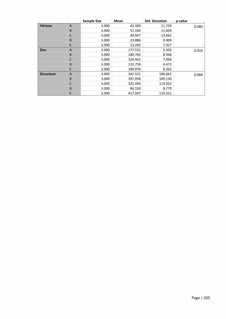
Page | 205
Sample Size Mean Std. Deviation ρ-value
Yttrium A 3.000 43.309 11.759 0.080
B 3.000 51.184 11.600
C 3.000 40.947 13.662
D 3.000 23.886 0.909
E 3.000 53.283 7.927
Zinc A 3.000 177.551 3.502 0.016
B 3.000 180.765 8.946
C 3.000 104.442 7.004
D 3.000 131.758 4.473
E 3.000 189.870 8.362
Zirconium A 3.000 342.521 106.661 0.084
B 3.000 397.058 109.130
C 3.000 325.494 119.052
D 3.000 84.150 8.770
E 3.000 417.047 110.321

Page | 206
Appendix 3: ICP-MS Results

Page | 207

Page | 208
Appendix 4: Shapiro-Wilk Test
Statistic Shapiro-Wilk
df ρ-value
Aluminium 0.961 101 0.005
Arsenic 0.671 101 0.000
Barium 0.660 101 0.000
Bismuth 0.907 101 0.000
Bromine 0.903 101 0.000
Calcium 0.978 101 0.096
Cadmium 0.825 101 0.000
Cerium 0.075 101 0.000
Chlorine 0.871 101 0.000
Cobalt 0.411 101 0.000
Chromium 0.545 101 0.000
Caesium 0.196 101 0.000
Copper 0.928 101 0.000
Iron 0.966 101 0.010
Gallium 0.833 101 0.000
Germanium 0.562 101 0.000
Iodine 0.802 101 0.000
Potassium 0.936 101 0.000
Lanthanum 0.303 101 0.000
Magnesium 0.829 101 0.000
Manganese 0.940 101 0.000
Molybdenum 0.863 101 0.000
Sodium 0.940 101 0.000
Niobium 0.875 101 0.000
Neodymium 0.171 101 0.000
Nickel 0.730 101 0.000
Phosphorus 0.964 101 0.007
Lead 0.708 101 0.000
Praseodymium 0.000 101 0.000
Rubidium 0.942 101 0.000
Antimony 0.797 101 0.000
Selenium 0.865 101 0.000
Silicon 0.917 101 0.000
Tin 0.922 101 0.000
Sulphur 0.760 101 0.000
Strontium 0.831 101 0.000
Tantalum 0.000 101 0.000
Tellurium 0.814 101 0.000
Titanium 0.957 101 0.003
Vanadium 0.447 101 0.000
Tungsten 0.134 101 0.000
Yttrium 0.922 101 0.000
Zinc 0.722 101 0.000
Zirconium 0.937 101 0.000

Page | 209
Appendix 5: One-Way ANOVA Test and Kruskal-Wallis Test (Districts)
Sample Size Mean Std. Deviation ρ-value
Aluminium Southern harbour 18 35071.630 8559.020 0.268
Northern harbour 12 30414.230 7095.803
South-Eastern 23 37756.230 10671.178
Western 18 38106.000 12018.356
Northern 15 36902.840 14210.091
Gozo and Comino 15 31737.360 9081.968
Arsenic Southern harbour 18 5.010 8.542 0.245
Northern harbour 12 1.330 4.591
South-Eastern 23 6.720 9.847
Western 18 7.030 8.878
Northern 15 7.930 11.743
Gozo and Comino 15 4.190 7.314
Barium Southern harbour 18 177.390 306.910 0.312
Northern harbour 12 46.800 133.231
South-Eastern 23 305.730 415.788
Western 18 224.460 323.458
Northern 15 251.260 364.011
Gozo and Comino 15 106.940 243.794
Bismuth Southern harbour 18 27.610 14.673 0.569
Northern harbour 12 23.550 9.624
South-Eastern 23 32.950 14.278
Western 18 29.400 14.067
Northern 15 32.110 19.275
Gozo and Comino 15 28.170 13.708
Bromine Southern harbour 18 36.560 16.019 0.197
Northern harbour 12 33.420 12.406
South-Eastern 23 40.520 11.920
Western 18 34.720 14.624
Northern 15 47.800 26.466
Gozo and Comino 15 34.130 11.538
Calcium Southern harbour 18 215397.000 30201.098 0.073
Northern harbour 12 227375.900 28405.988
South-Eastern 23 202428.800 31510.428
Western 18 201035.700 36833.081
Northern 15 200924.400 44806.688
Gozo and Comino 15 216528.100 40285.145
Cadmium Southern harbour 18 17.910 17.952 0.560
Northern harbour 12 16.690 17.912
South-Eastern 23 28.950 22.077
Western 18 24.690 20.197
Northern 15 30.100 22.876
Gozo and Comino 15 22.720 20.113
Cerium Southern harbour 18 4.430 18.804 0.437
Northern harbour 12 0.000 0.000
South-Eastern 23 0.000 0.000
Western 18 0.000 0.000
Northern 15 0.000 0.000
Gozo and Comino 15 0.000 0.000

Page | 210
Sample Size Mean Std. Deviation ρ-value
Chlorine Southern harbour 18 2697.220 358.966 0.263
Northern harbour 12 2529.170 386.181
South-Eastern 23 2847.390 594.92
Western 18 2683.330 392.593
Northern 15 2886.670 648.092
Gozo and Comino 15 2792.670 649.169
Cobalt Southern harbour 18 7.560 22.372 0.437
Northern harbour 12 0.000 0.00
South-Eastern 23 8.650 27.134
Western 18 3.760 12.657
Northern 15 4.300 16.652
Gozo and Comino 15 15.830 20.823
Chromium Southern harbour 18 25.700 51.943 0.450
Northern harbour 12 21.950 37.163
South-Eastern 23 45.930 72.310
Western 18 12.390 45.394
Northern 15 18.790 33.130
Gozo and Comino 15 8.990 34.802
Caesium Southern harbour 18 7.810 33.142 0.832
Northern harbour 12 0.000 0.000
South-Eastern 23 5.860 28.083
Western 18 6.640 28.151
Northern 15 0.000 0.000
Gozo and Comino 15 5.480 21.215
Copper Southern harbour 18 95.150 56.719 0.042
Northern harbour 12 45.600 47.032
South-Eastern 23 70.990 47.609
Western 18 70.650 41.594
Northern 15 54.910 71.596
Gozo and Comino 15 39.620 41.249
Iron Southern harbour 18 25509.770 8194.762 0.356
Northern harbour 12 21769.760 6729.687
South-Eastern 23 28810.430 12239.424
Western 18 28797.090 12020.045
Northern 15 27385.020 10283.350
Gozo and Comino 15 27618.160 8184.606
Gallium Southern harbour 18 13.180 13.490 0.247
Northern harbour 12 5.390 11.495
South-Eastern 23 14.780 15.247
Western 18 15.660 14.941
Northern 15 14.830 16.036
Gozo and Comino 15 8.230 11.107
Germanium Southern harbour 18 3.390 6.313 0.768
Northern harbour 12 1.270 3.320
South-Eastern 23 2.810 5.226
Western 18 2.080 3.650
Northern 15 4.400 7.289
Gozo and Comino 15 0.230 0.896
Iodine Southern harbour 18 29.390 41.930 0.373
Northern harbour 12 25.670 35.395
South-Eastern 23 53.700 46.061
Western 18 43.560 47.123
Northern 15 62.200 54.219
Gozo and Comino 15 35.130 43.858

Page | 211
Sample Size Mean Std. Deviation ρ-value
Potassium Southern harbour 18 10249.590 2751.518 0.164
Northern harbour 12 8557.460 1827.554
South-Eastern 23 9975.520 2724.678
Western 18 10623.610 3994.561
Northern 15 11914.870 4704.408
Gozo and Comino 15 10710.600 2587.749
Lanthanum Southern harbour 18 46.940 136.658 0.991
Northern harbour 12 44.060 152.611
South-Eastern 23 29.320 97.688
Western 18 7.720 23.772
Northern 15 50.190 140.304
Gozo and Comino 15 0.000 0.000
Magnesium Southern harbour 18 12637.040 5135.293 0.216
Northern harbour 12 13869.920 5829.532
South-Eastern 23 14931.790 4023.22
Western 18 15555.080 4735.913
Northern 15 12675.90 5958.04
Gozo and Comino 15 16981.610 5582.731
Manganese Southern harbour 18 463.390 214.253 0.118
Northern harbour 12 368.130 171.558
South-Eastern 23 586.670 264.078
Western 18 560.750 279.624
Northern 15 487.450 286.52
Gozo and Comino 15 374.680 156.732
Molybdenum Southern harbour 18 7.810 7.178 0.134
Northern harbour 12 5.550 6.025
South-Eastern 23 11.850 7.739
Western 18 9.000 7.154
Northern 15 12.090 9.037
Gozo and Comino 15 6.800 7.046
Sodium Southern harbour 18 88648.150 24915.083 0.647
Northern harbour 12 96138.870 22118.480
South-Eastern 23 97399.770 18815.25
Western 18 102088.200 24897.879
Northern 15 97233.120 41676.865
Gozo and Comino 15 100398.400 42850.892
Niobium Southern harbour 18 16.820 11.881 0.065
Northern harbour 12 13.510 9.950
South-Eastern 23 24.070 12.428
Western 18 19.570 12.818
Northern 15 25.860 15.413
Gozo and Comino 15 16.310 10.841
Neodymium Southern harbour 18 13.050 55.370 0.217
Northern harbour 12 0.000 0.000
South-Eastern 23 18.380 59.747
Western 18 0.000 0.000
Northern 15 0.000 0.000
Gozo and Comino 15 0.000 0.000
Nickel Southern harbour 18 19.950 23.176 0.060
Northern harbour 12 2.490 8.620
South-Eastern 23 21.900 24.852
Western 18 16.070 18.676
Northern 15 12.470 19.328
Gozo and Comino 15 5.710 15.787

Page | 212
Sample Size Mean Std. Deviation ρ-value
Phosphorus Southern harbour 18 4247.580 1044.356 0.148
Northern harbour 12 3574.280 1534.899
South-Eastern 23 3437.850 797.069
Western 18 3549.060 1133.783
Northern 15 3552.750 934.537
Gozo and Comino 15 3958.330 1003.054
Lead Southern harbour 18 249.510 175.818 0.000
Northern harbour 12 114.260 56.064
South-Eastern 23 150.310 64.146
Western 18 107.320 43.958
Northern 15 69.810 25.163
Gozo and Comino 15 62.260 40.823
Praseodymium Southern harbour 18 0.000 0.000 1.000
Northern harbour 12 0.000 0.000
South-Eastern 23 0.000 0.000
Western 18 0.000 0.000
Northern 15 0.000 0.000
Gozo and Comino 15 0.000 0.000
Rubidium Southern harbour 18 70.410 27.868 0.145
Northern harbour 12 61.720 21.468
South-Eastern 23 84.720 31.453
Western 18 83.210 39.181
Northern 15 82.240 34.863
Gozo and Comino 15 76.020 23.578
Antimony Southern harbour 18 39.080 47.019 0.663
Northern harbour 12 33.070 40.044
South-Eastern 23 59.710 54.285
Western 18 54.300 50.664
Northern 15 66.610 60.078
Gozo and Comino 15 20.490 39.687
Selenium Southern harbour 18 11.540 8.524 0.336
Northern harbour 12 9.130 6.029
South-Eastern 23 15.500 9.070
Western 18 12.060 8.768
Northern 15 15.510 11.320
Gozo and Comino 15 10.110 6.921
Silicon Southern harbour 18 115700.800 29994.255 0.460
Northern harbour 12 101614.300 19665.228
South-Eastern 23 119826.400 32131.894
Western 18 118199.600 29271.378
Northern 15 126948.800 52284.641
Gozo and Comino 15 102132.400 22299.761
Tin Southern harbour 18 131.540 27.589 0.259
Northern harbour 12 117.760 22.199
South-Eastern 23 141.130 28.152
Western 18 131.670 28.562
Northern 15 136.160 36.163
Gozo and Comino 15 122.140 25.164
Sulphur Southern harbour 18 2122.870 416.356 0.382
Northern harbour 12 1825.610 287.361
South-Eastern 23 1988.570 321.828
Western 18 1917.730 400.863
Northern 15 2058.040 396.061
Gozo and Comino 15 2218.770 1004.911

Page | 213
Sample Size Mean Std. Deviation ρ-value
Strontium Southern harbour 18 289.760 30.699 0.008
Northern harbour 12 340.350 54.273
South-Eastern 23 276.210 50.524
Western 18 271.720 122.935
Northern 15 279.950 87.329
Gozo and Comino 15 433.900 153.972
Tantalum Southern harbour 18 0.000 0.000 1.000
Northern harbour 12 0.000 0.000
South-Eastern 23 0.000 0.000
Western 18 0.000 0.000
Northern 15 0.000 0.000
Gozo and Comino 15 0.000 0.000
Tellurium Southern harbour 18 33.530 38.222 0.358
Northern harbour 12 28.920 30.455
South-Eastern 23 52.730 43.039
Western 18 43.530 40.575
Northern 15 63.210 49.286
Gozo and Comino 15 43.010 38.958
Titanium Southern harbour 18 2780.600 782.126 0.503
Northern harbour 12 2494.250 1090.385
South-Eastern 23 3121.260 1204.085
Western 18 2906.230 1157.672
Northern 15 2868.440 1235.728
Gozo and Comino 15 2360.200 808.672
Vanadium Southern harbour 18 18.640 55.276 0.336
Northern harbour 12 10.410 36.061
South-Eastern 23 64.250 151.056
Western 18 41.450 84.732
Northern 15 51.010 77.864
Gozo and Comino 15 10.760 41.655
Tungsten Southern harbour 18 1.230 5.233 0.590
Northern harbour 12 0.000 0.000
South-Eastern 23 0.000 0.000
Western 18 0.880 3.738
Northern 15 0.000 0.000
Gozo and Comino 15 0.160 0.614
Yttrium Southern harbour 18 29.840 14.140 0.033
Northern harbour 12 28.940 10.777
South-Eastern 23 43.340 15.618
Western 18 31.450 14.038
Northern 15 34.750 17.239
Gozo and Comino 15 29.560 9.444
Zinc Southern harbour 18 251.330 210.663 0.187
Northern harbour 12 160.350 113.805
South-Eastern 23 172.450 67.316
Western 18 158.810 55.181
Northern 15 173.480 145.836
Gozo and Comino 15 128.120 74.940
Zirconium Southern harbour 18 279.100 140.888 0.136
Northern harbour 12 248.560 136.316
South-Eastern 23 388.250 174.769
Western 18 303.570 154.017
Northern 15 355.900 188.420
Gozo and Comino 15 212.180 102.137

Page | 214
Appendix 6: Sample A
Sample A 1st try 2nd try 3rd try Average
Aluminium 27256.375 26621.275 26885.900 26921.183
Arsenic 0.000 0.000 22.722 7.574
Barium 0.000 0.000 625.164 208.388
Bismuth 23.322 21.528 53.819 32.890
Bromine 28.000 28.000 52.000 36.000
Calcium 224837.580 229646.940 225639.140 226707.887
Cadmium 12.298 11.419 48.312 24.010
Cerium 0.000 0.000 0.000 0.000
Chlorine 2170.000 2100.000 2780.000 2350.000
Cobalt 0.000 0.000 0.000 0.000
Chromium 0.000 0.000 0.000 0.000
Caesium 0.000 0.000 0.000 0.000
Copper 79.886 97.461 113.438 96.928
Iron 23640.734 23430.905 23850.563 23640.734
Gallium 2.976 9.671 27.525 13.391
Germanium 2.083 3.471 0.000 1.851
Iodine 12.000 4.000 107.000 41.000
Potassium 8633.560 8467.530 11373.055 9491.382
Lanthanum 0.000 0.000 0.000 0.000
Magnesium 15437.824 13327.184 14352.352 14372.453
Manganese 392.651 408.140 542.896 447.896
Molybdenum 11.331 5.332 21.329 12.664
Sodium 102376.680 98667.380 94958.080 98667.380
Niobium 18.175 11.884 34.253 21.437
Neodymium 0.000 0.000 0.000 0.000
Nickel 0.000 0.000 33.789 11.263
Phosphorus 4538.768 3740.119 4049.978 4109.622
Lead 143.890 141.105 109.542 131.512
Praseodymium 0.000 0.000 0.000 0.000
Rubidium 64.923 63.094 81.382 69.800
Antimony 33.414 24.225 135.327 64.322
Selenium 8.539 8.539 27.042 14.707
Silicon 100021.560 100021.560 102569.880 100871.000
Tin 115.789 107.124 165.413 129.442
Sulphur 1565.955 1642.050 2086.605 1764.870
Strontium 345.846 336.545 343.310 341.900
Tantalum 0.000 0.000 0.000 0.000
Tellurium 31.181 16.790 112.730 53.567
Titanium 2673.056 2726.997 2691.037 2697.030
Vanadium 0.000 0.000 0.000 0.000
Tungsten 0.000 0.000 0.000 0.000
Yttrium 38.585 34.647 56.696 43.309
Zinc 173.534 179.158 179.962 177.551
Zirconium 293.167 269.476 464.921 342.521

Page | 215
Appendix 7: Sample B
Sample B 1st try 2nd try 3rd try Average
Aluminium 28526.575 27573.925 30431.875 28844.125
Arsenic 21.964 0.000 15.905 12.623
Barium 789.068 0.000 532.016 440.361
Bismuth 51.128 18.837 43.056 37.674
Bromine 61.000 34.000 50.000 48.333
Calcium 224036.020 236059.420 219226.660 226440.700
Cadmium 57.096 11.419 43.920 37.478
Cerium 0.000 0.000 0.000 0.000
Chlorine 2740.000 2110.000 2640.000 2496.667
Cobalt 0.000 0.000 0.000 0.000
Chromium 0.000 0.000 0.000 0.000
Caesium 148.234 0.000 85.552 77.929
Copper 115.036 81.484 95.863 97.461
Iron 25319.366 25249.423 25878.910 25482.566
Gallium 28.269 0.000 17.110 15.127
Germanium 14.578 0.000 7.636 7.405
Iodine 128.000 0.000 88.000 72.000
Potassium 13199.385 9048.635 11954.160 11400.727
Lanthanum 0.000 0.000 0.000 0.000
Magnesium 14412.656 13266.880 15799.648 14493.061
Manganese 603.304 460.804 517.339 527.149
Molybdenum 22.662 7.332 15.330 15.108
Sodium 93474.360 89765.060 89023.200 90754.207
Niobium 38.447 14.680 27.962 27.030
Neodymium 0.000 0.000 0.000 0.000
Nickel 40.076 0.000 16.502 18.859
Phosphorus 4669.694 3587.372 4451.484 4236.183
Lead 81.692 114.183 89.119 94.998
Praseodymium 0.000 0.000 0.000 0.000
Rubidium 86.869 67.666 80.468 78.334
Antimony 147.022 28.402 116.114 97.179
Selenium 29.176 6.405 21.349 18.977
Silicon 99384.480 93650.760 108940.680 100658.640
Tin 184.317 115.789 161.474 153.860
Sulphur 2334.915 1610.010 2162.700 2035.875
Strontium 347.537 345.001 346.692 346.410
Tantalum 0.000 0.000 0.000 0.000
Tellurium 120.725 14.391 89.544 74.887
Titanium 2798.918 2774.944 2834.878 2802.913
Vanadium 65.540 0.000 2.241 22.594
Tungsten 0.000 0.000 0.000 0.000
Yttrium 61.420 38.585 53.546 51.184
Zinc 188.799 171.124 182.372 180.765
Zirconium 501.197 283.543 406.436 397.058

Page | 216
Appendix 8: Sample C
Sample C 1st try 2nd try 3rd try Average
Aluminium 19264.700 22069.725 23869.175 21734.533
Arsenic 19.692 0.000 0.000 6.564
Barium 663.677 0.000 0.000 221.226
Bismuth 45.746 40.365 15.249 33.787
Bromine 50.000 50.000 25.000 41.667
Calcium 261709.340 233654.740 234456.300 243273.460
Cadmium 51.826 51.826 8.784 37.478
Cerium 0.000 0.000 0.000 0.000
Chlorine 2600.000 2500.000 2030.000 2376.667
Cobalt 11.797 0.000 0.000 3.932
Chromium 0.000 0.000 0.000 0.000
Caesium 0.000 0.000 0.000 0.000
Copper 107.047 116.634 82.283 101.988
Iron 17275.921 17136.035 16856.263 17089.406
Gallium 22.318 0.000 0.000 7.439
Germanium 0.000 0.000 0.000 0.000
Iodine 100.000 102.000 12.000 71.333
Potassium 8384.515 8201.882 7014.768 7867.055
Lanthanum 246.425 0.000 0.000 82.142
Magnesium 12422.624 20443.056 14111.136 15658.939
Manganese 381.034 407.366 242.406 343.602
Molybdenum 18.663 18.663 2.666 13.331
Sodium 100151.100 135760.380 116472.020 117461.167
Niobium 31.457 30.758 8.388 23.534
Neodymium 0.000 0.000 0.000 0.000
Nickel 13.359 0.000 0.000 4.453
Phosphorus 3033.119 2779.995 3395.348 3069.487
Lead 62.197 71.481 94.689 76.122
Praseodymium 0.000 0.000 0.000 0.000
Rubidium 59.437 58.522 42.063 53.341
Antimony 124.467 119.455 30.073 91.332
Selenium 24.907 21.349 6.405 17.553
Silicon 63198.336 66256.320 87917.040 72457.232
Tin 162.262 157.536 117.364 145.721
Sulphur 1898.370 1750.185 1718.145 1788.900
Strontium 340.773 333.162 339.082 337.672
Tantalum 0.000 0.000 0.000 0.000
Tellurium 99.938 96.740 17.589 71.422
Titanium 1792.027 3044.647 1971.829 2269.501
Vanadium 73.382 0.000 0.000 24.461
Tungsten 0.000 0.000 0.000 0.000
Yttrium 49.609 48.034 25.198 40.947
Zinc 107.656 109.262 96.408 104.442
Zirconium 392.370 396.071 188.041 325.494

Page | 217
Appendix 9: Sample D
Sample D 1st try 2nd try 3rd try Average
Aluminium 12913.700 13178.325 13919.275 13337.100
Arsenic 0.000 0.000 0.000 0.000
Barium 0.000 0.000 0.000 0.000
Bismuth 17.940 14.352 12.558 14.950
Bromine 31.000 30.000 28.000 29.667
Calcium 273331.960 270125.720 270526.500 271328.060
Cadmium 3.514 3.514 4.392 3.806
Cerium 0.000 0.000 0.000 0.000
Chlorine 1930.000 1880.000 1750.000 1853.333
Cobalt 0.000 0.000 0.000 0.000
Chromium 0.000 0.000 0.000 0.000
Caesium 0.000 0.000 0.000 0.000
Copper 74.294 54.322 50.328 59.648
Iron 11470.652 11610.538 11120.937 11400.709
Gallium 0.000 0.000 0.000 0.000
Germanium 0.000 0.000 0.000 0.000
Iodine 20.000 13.000 10.000 14.333
Potassium 5537.101 4665.443 4748.458 4983.667
Lanthanum 0.000 0.000 0.000 0.000
Magnesium 14834.784 16402.688 16221.776 15819.749
Manganese 157.215 147.147 124.688 143.017
Molybdenum 2.666 3.333 2.000 2.666
Sodium 113504.580 120181.320 114246.440 115977.447
Niobium 5.592 6.291 4.893 5.592
Neodymium 0.000 0.000 0.000 0.000
Nickel 0.000 0.000 0.000 0.000
Phosphorus 3945.237 3823.039 3919.052 3895.776
Lead 155.029 153.173 152.244 153.482
Praseodymium 0.000 0.000 0.000 0.000
Rubidium 32.919 32.919 30.176 32.004
Antimony 35.085 34.249 25.896 31.743
Selenium 6.405 4.981 5.693 5.693
Silicon 47526.168 47016.504 50902.692 48481.788
Tin 107.912 107.124 107.912 107.650
Sulphur 1638.045 1389.735 1457.820 1495.200
Strontium 501.435 508.200 502.280 503.972
Tantalum 0.000 0.000 0.000 0.000
Tellurium 23.985 21.587 18.389 21.320
Titanium 887.023 713.215 617.320 739.186
Vanadium 0.000 0.000 0.000 0.000
Tungsten 0.000 0.000 0.000 0.000
Yttrium 24.411 24.411 22.836 23.886
Zinc 136.578 127.741 130.954 131.758
Zirconium 88.838 89.579 74.032 84.150

Page | 218
Appendix 10: Sample E
Sample E 1st try 2nd try 3rd try Average
Aluminium 27468.075 27944.400 30961.125 28791.200
Arsenic 18.177 0.000 25.751 14.643
Barium 402.147 0.000 775.633 392.593
Bismuth 43.953 25.116 60.098 43.056
Bromine 69.000 55.000 81.000 68.333
Calcium 229646.940 189568.940 206802.480 208672.787
Cadmium 46.555 26.352 57.096 43.334
Cerium 0.000 0.000 0.000 0.000
Chlorine 3310.000 2810.000 3750.000 3290.000
Cobalt 0.000 0.000 0.000 0.000
Chromium 0.000 0.000 0.000 0.000
Caesium 0.000 0.000 139.763 46.588
Copper 93.467 79.886 131.812 101.722
Iron 26158.682 27487.599 26648.283 26764.855
Gallium 18.598 5.951 31.989 18.846
Germanium 7.636 2.083 0.000 3.240
Iodine 64.000 3.000 127.000 64.667
Potassium 11373.055 8882.605 14444.610 11566.757
Lanthanum 0.000 0.000 0.000 0.000
Magnesium 15317.216 23518.560 16945.424 18593.733
Manganese 526.633 495.654 616.470 546.252
Molybdenum 14.664 11.331 22.662 16.219
Sodium 91248.780 163951.060 97925.520 117708.453
Niobium 27.962 18.874 37.049 27.962
Neodymium 0.000 0.000 0.000 0.000
Nickel 23.574 0.000 44.005 22.526
Phosphorus 3927.780 3517.545 4756.978 4067.434
Lead 90.975 124.395 89.119 101.496
Praseodymium 0.000 0.000 0.000 0.000
Rubidium 79.554 71.324 89.612 80.163
Antimony 0.000 0.000 144.516 48.172
Selenium 21.349 9.251 30.600 20.400
Silicon 94924.920 89191.200 112763.160 98959.760
Tin 146.508 116.577 178.016 147.034
Sulphur 2635.290 2230.785 3204.000 2690.025
Strontium 347.537 368.677 351.765 355.993
Tantalum 0.000 0.000 0.000 0.000
Tellurium 71.156 6.396 114.329 63.960
Titanium 2810.905 3218.456 2906.799 2978.720
Vanadium 25.768 0.000 90.748 38.838
Tungsten 0.000 0.000 0.000 0.000
Yttrium 54.333 44.884 60.633 53.283
Zinc 183.175 187.192 199.243 189.870
Zirconium 406.436 312.415 532.290 417.047

Page | 219
Appendix 11: Southern Harbour Samples

Page | 220
Appendix 12: Northern Harbour Samples
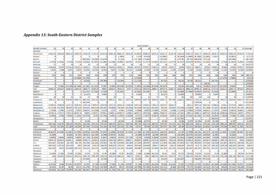
Page | 221
Appendix 13: South-Eastern District Samples
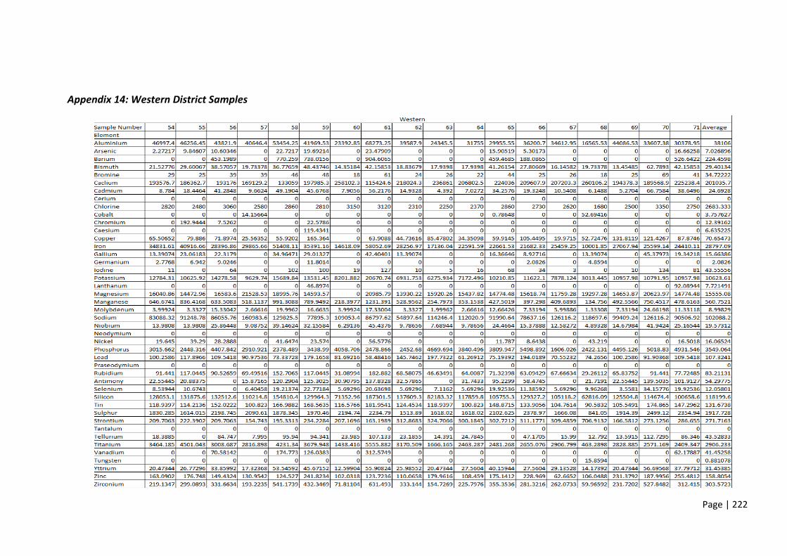
Page | 222
Appendix 14: Western District Samples

Page | 223
Appendix 15: Northern District Samples
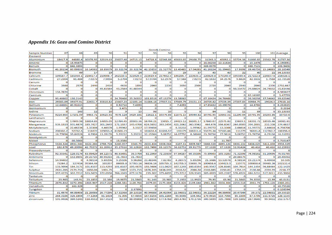
Page | 224
Appendix 16: Gozo and Comino District

Page | 225
Appendix 17: Example of XRF graph with a chromium peak but a 0 ppm value