Handling of Complex Nmnbers in the CH Progrannning Language

HARRY H. CHENG Department of Mechanical and Aeronautical Engineering, University of California, Davis, CA 95616

ABSTRACT

The handling of complex numbers in the (H programming language will be described in this paper. Complex is a built-in data type in (H. The 1/0, arithmetic and relational operations, and built-in mathematical functions are defined for both regular complex numbers and complex metanumbers of ComplexZero, Complexlnf, and ComplexNaN. Due to polymorphism, the syntax of complex arithmetic and relational operations and built-in mathematical functions are the same as those for real numbers. Besides poly­morphism, the built-in mathematical functions are implemented with a variable number of arguments that greatly simplify computations of different branches of multiple-valued complex functions. The valid lvalues related to complex numbers are defined. Ration­ales for the design of complex features in (H are discussed from language design, implementation, and application points of views. Sample (H programs show that a computer language that does not distinguish the sign of zeros in complex numbers can also handle the branch cuts of multiple-valued complex functions effectively so long as it is appropriately designed and implemented. © 1994 John Wiley & Sons, Inc.

1 INTRODUCTION

Cheng [ 1] presented the extension of C to CH, a general-purpose block-structured interpretive programming language for the numerical compu­tation of real numbers. The extension of scientific programming from the one-dimensional real line to the two-dimensional extended complex plane will be described in this article. Complex number, an extension of real number, has wide applica­tions in science and engineering. Due to its impor­tance in scientific programming, numerically ori­ented programming languages and software

Received October 1992 Revised May 1993

© 1994 by John Wiley & Sons, Inc. Scientific Programming, Vol. 2, pp. 77-106 (1993) CCC 1058-9244/94/030077-30

packages usually provide complex number sup­port in one way or another. For example, Fortran [2], a language mainly for scientific computing, has provided complex data type since its earliest days. Ada has introduced complex data in its new proposed standard recently [3-6, 38]. C, a mod­ern language originally invented for the Unix sys­tem programming [7, 8], does not have complex as a basic data type because the numerically ori­ented scientific computing was not its original de­sign goal. Computations involving complex num­bers can be introduced as a data structure in C. However, programming with this structure is somewhat clumsy because, for each operation, a corresponding function has to be invoked. Using c++ [9], a class for complex numbers can be cre­ated. By using operator and funtion overloadings, built-in operators and functions can be extended so as to also apply to the complex data type. Therefore, the complex data type can be

77

78 CHENG

achieved. However, it may be too involved for novice users to create such a class. Besides, many features described in this article cannot be con­veniently implemented at the user's level.

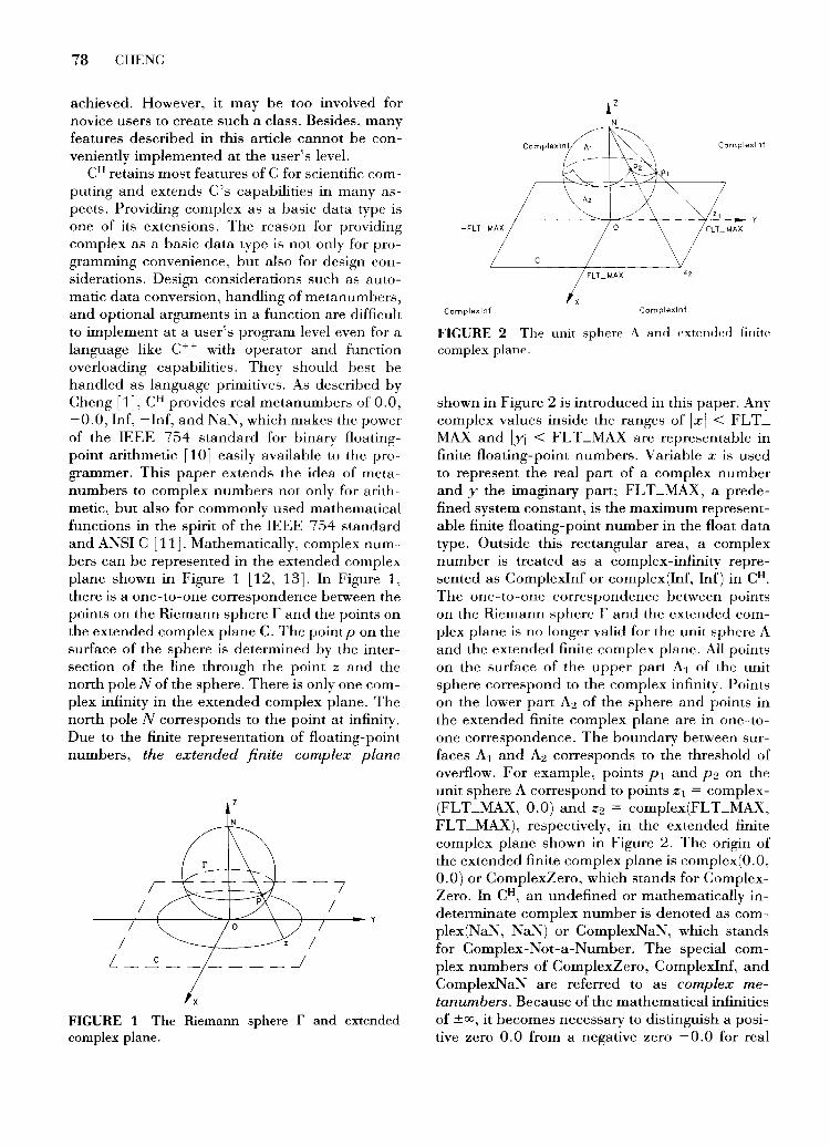
CH retains most features of C for scientific com­puting and extends C's capabilities in many as­pects. Providing complex as a basic data type is one of its extensions. The reason for providing complex as a basic data type is not only for pro­gramming convenience, but also for design con­siderations. Design considerations such as auto­matic data conversion, handling of metanumbers, and optional arguments in a function are difficult to implement at a user's program level even for a language like c++ with operator and function overloading capabilities. They should best be handled as language primitives. As described by Cheng [1], CH provides real metanumbers of 0.0, -0.0, lnf,- lnf, and 1'\aN, which makes the power of the IEEE 754 standard for binary floating­point arithmetic [10] easily available to the pro­grammer. This paper extends the idea of meta­numbers to complex numbers not only for arith­metic, but also for commonly used mathematical functions in the spirit of the IEEE 754 standard and ANSI C [11]. Mathematically, complex num­bers can be represented in the extended complex plane shown in Figure 1 [12, 13]. In Figure 1, there is a one-to-one correspondence between the points on the Riemann sphere r and the points on the extended complex plane C. The point p on the surface of the sphere is determined by the inter­section of the line through the point z and the north pole N of the sphere. There is only one com­plex infinity in the extended complex plane. The north pole N corresponds to the point at infinity. Due to the finite representation of floating-point numbers, the extended finite complex plane

z

N

FIGURE 1 The Riemann sphere r and extended complex plane.

z

N

c FLT_MAX Zz

Complexlnf Complexlnf

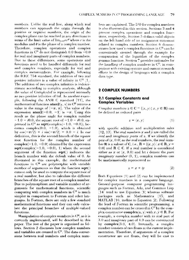
FIGURE 2 The unit sphere A and extended finite complex plane.

shown in Figure 2 is introduced in this paper. Any complex values inside the ranges of lxl < FL T_ MAX and IYI < FL T _MAX are representable in finite floating-point numbers. Variable x is used to represent the real part of a complex number and y the imaginary part; FL T _MAX, a prede­fined system constant, is the maximum represent­able finite floating-point number in the float data type. Outside this rectangular area, a complex number is treated as a complex-infinity repre­sented as Complexlnf or complex(lnf, Inf) in CH. The one-to-one correspondence between points on the Riemann sphere rand the extended com­plex plane is no longer valid for the unit sphere A and the extended finite complex plane. All points on the surface of the upper part A1 of the unit sphere correspond to the complex infinity. Points on the lower part A2 of the sphere and points in the extended finite complex plane are in one-to­one correspondence. The boundary between sur­faces A1 and A2 corresponds to the threshold of overflow. For example, points p1 and P2 on the unit sphere A correspond to points z1 = complex­(FLT_MAX, 0.0) and z2 = complex(FLT_MAX, FLT_MAX), respectively, in the extended finite complex plane shown in Figure 2. The origin of the extended finite complex plane is complex(O.O, 0.0) or ComplexZero, which stands for Complex­Zero. In CH, an undefined or mathematically in­determinate complex number is denoted as com­plex(NaN, NaN) or ComplexNaN, which stands for Complex-Not-a-Number. The special com­plex numbers of ComplexZero, Complexlnf, and ComplexNaN are referred to as complex me­tanumbers. Because of the mathematical infinities of ±oo, it becomes necessary to distinguish a posi­tive zero 0.0 from a negative zero -0.0 for real

CO.VIPLEX "JL.V1BERS L'\ C11 PROGRA.VIYII."JG LA."JGLAGE 79

numbers. Cnlike the real line, along which real numbers can approach the origin through the positive or negative numbers, the origin of the complex plane can be reached in any directions in terms of the limit value of lim,.._.0 re;0 where r is the modulus and (J is the phase of a complex number. Therefore, complex operations and complex functions in CH do not distinguish 0.0 from -0.0 for real and imaginary parts of complex numbers. Due to these differences, some operations and functions need to be handled differently for real and complex numbers, especially for real and complex metanumbers. For example, following the IEEE 754 standard, the addition of two real positive infinities is a value of infinity in CH [ 1]. The addition of two complex infinities is indeter­minate according to complex analysis, although the value of Complexlnf is represented intemally as two positive infinities of Inf. As another exam­ple, following the ANSI C standard [ 11], the mathematical function atan2(y, x) inCH retums a value in the range of [ -7r, 1T ]. The value of the expression atan2 (- 0. 0, -1) is -7r. Using this result as the phase angle for complex number -1.0- iO.O, the square root of -1.0- iO.O, ex­pressed inCH as sqrt(complex(-1.0, -0.0)), be­comes complex(O.O, -1.0), which is obtained by cos(-7T/2) + i sin(-'TT/2) = 0.0 - i. In our definition, this is the second branch of the square root function for the complex number of complex(-1.0, -0.0) obtained by the expression sqrt(complex(-1.0, -0.0), 1) where the second argument of the function sqrt() indicates the branch number with the default value of 0. As illustrated in this example, the mathematical functions in CH are polymorphic with variable number of arguments so that the function sqrt() cannot only be used to compute the square root of a real number, but also to calculate the different branches of the square root of a complex number. Due to polymorphism and variable number of ar­guments for mathematical functions, scientific computing with complex numbers in CH is much simpler in comparison to Fortran and other lan­guages. In Fortran, there are only a few standard mathematical functions and they can only calcu­late the principal branches of multiple-valued functions.

Manipulation of complex numbers in CH, as it is currently implemented, will be described in this paper. The rest of the paper is organized as fol­lows. Section 2 discusses how complex numbers and variables are created inCH. The data conver­sions between real numbers and complex num-

hers are explained. The 1/0 for complex numbers is also illustrated in this section. Sections 3 and 4 present complex operations and complex func­tions, respectively. Section 5 defines valid objects on the left hand side of an assignment statement related to complex numbers. Section 6 demon­strates how user's complex functions inCH can be conveniently created through the example for computation of the logarithm of the complex gamma function. Section 7 provides rationales for the handling of complex numbers in CH, in com­parison with existing systems and current research efforts in the design of languages with a complex data type.

2 COMPLEX NUMBERS

2.1 Complex Constants and Complex Variables

Complex numbers z E C = {(x, y) I x, y E R} can be defined as ordered pairs

z = (x,y) (1)

with specific addition and multiplication rules [12, 13]. The real numbers x andy are called the real and imaginary parts of z. If we identify the pair of (x, 0.0) as the real numbers, the real num­ber R is a subset of C, i.e., R = {(x, y) I x E R, y = 0.0} and R C C. If a real number is considered either as x or (x, 0.0) and let i denote the pure imaginary number (0, 1), complex numbers can be mathematically represented as

Z =X+ iy (2)

Both Equations (1) and (2) can be implemented for complex numbers in a computer language. General-purpose computer programming lan­guages such as Fortran, Ada, and Common Lisp [14] tend to use Equation (1) whereas software packages such as Mathematica [15] and MATLAB [16] incline to Equation (2). Following the lead of Fortran in scientific programming, a complex number can be created inCH by the com­plex constructor complex(x, y) with x, y E R. For example, a complex number with its real part of 3.0 and imaginary part of 4.0 can be constructed by complex(3.0, 4.0). lntemally, a complex number consists of two floats at the current imple­mentation. Therefore, if arguments of a complex constructor are not floats, they will be cast to

80 CHENG

floats internally. As described by Cheng [ 1], all floating-point constants in CH are floats by de­fault. The double constants can be obtained by suffixing a floating-point constant with D or d. When double complex data type is implemented in the future, the complex constructor shall return complex or double complex polymorphically, de­pending on the data types of the input arguments. For example, complex(3, 4.0d), complex(3.0f, 4.0d), complex(3.0D, 4.0F), and com­plex(3.0D, 4.0D) shall return a double complex number of complex(3.0D, 4.0D). By default, complex, Complexzero, Complexinf, and ComplexNaN are keywords inCH. However, as de­scribed by Cheng [ 1 J, these keywords can be changed at user's discretion. For example, one can add CMPLX to the keyword list and remove complex from the list by addkey ( "CMPLX",

be checked for compatibility. If data types do not match, the system will signal an error and print out some informative messages for the conven­ience of program debugging. However, unlike lan­guages such as Pascal [17], which prohibits auto­matic type conversion, some data type conversion rules have been built into CH so that they can be invoked whenever necessary. This will save many explicit type conversion commands for a program. The order of the data type in CH is arranged as

data type order

complex ri@ double float int char low

complex zl; /* declare zl as complex variable */ complex *zptrl; /* declare zptrl as pointer to complex variable */ complex z2[2], z3[2,3] ;I* declare z2 and z3 as arrays of complex*/ complex *zptr2[2] [4]; /*declare zptr2 as an array of pointer to complex*/ zptlr = &zl; /* zptrl point to the address of zl *zptrl = complex(1,2); /* zl becomes l+i2 */

"complex") andremkey("complex"), respec­tively. With this keyword change from complex to CMPLX, CMPLX will act the same as complex in a CH program in both syntax and semantics. Hence, porting code related to complex numbers from Fortran to CHis relatively easy. Many C programs have defined complex as the definition of a struc­ture for complex numbers. With the keyword changeability, reserved word conflict can be avoided when porting C programs to CH.

One can declare not only a simple complex variable, but also pointer to complex, array of complex, and array of pointer to complex, etc. Declarations of these complex variables are simi­lar to the declarations of any other data types in C. The array and pointer of complex in CH are ma­nipulated in the same manner as the floating­point float and double. The above code segment illustrates how complex is declared and manipu­lated inCH.

2.2 Data Conversion Rules

CH is a loosely typed language. All arguments of calling functions will be checked for compatibility with the data types of the called functions. The data types of operands for an operation will also

with char being the lowest data type and complex the highest data type. The default conversion rules will be brieflv discussed in this section as follows:

1. Char, int, float, and double can be con­verted according to ANSI C data conversion rules. The ASCII value of a character will be used in conversion for a char data type. De­motion of data may lose the information.

2. Char, int, float, and double can be con­verted to complex with its imaginary part being zero. When casting a real number into a complex number, the values of Inf and - Inf become Complexlnf: and the value of NaN becomes ComplexNal\. Conversion from double to complex may lose the infor­mation. A real number can be cast into a complex explicitly by the complex construc­tion function complex(x, y), which will be discussed in detail in Section 4.

3. When a complex is converted to char, int, float, and double, only its real part is used and the imaginary part will be discarded if the imaginary part of the complex is identi­cally zero. If the imaginary part of the com­plex is not identically zero, the converted

COMPLEX NUMBERS 1:"1 C" PROGRAMMING LANGUAGE 81

real number becomes NaN. The real and imaginary components of a complex num­ber can be obtained explicitly by the func­tions real(z) and imaginary(z), which will be discussed in detail in Section 4. When a complex number is converted to a real num­ber either implicitly by assignment state­ment such as f = z or explicitly by real(z), imaginary(z), float(z), double(z), (float)z, and (double)z, the sign of a zero wil not be carried over. Converting a complex number to an integral value such as char and int is equivalent to conversion of real(z) to an integral value if the imaginary part of the complex is identically zero. For example, i = Complexlnf will make i equal to INT_MAX. However, if real() or imagi­nary() is used as an lvalue, the sign of zeros from rvalue will be preserved, which will al­low experimentation with signed zeros in computations of complex numbers. An !value is any object that occurs on the left hand side of an assignment statement. The lvalue refers to a memorv such as a variable or pointer, not a function or constant. On the other hand, the rvalue refers to the value of the expression on the right hand side of an assignment statement. Details about the lvalue will be discussed in Section 5.

4. In binary operations such as addition, sub­traction, multiplication, and division, with mixed data types, the result of the operation will carry the higher data type of two oper­ands. For example, the result of addition of

an int and a double will result in a double. When one of the two binary operands is complex and the data type of other operand is a real number, the real number will be cast into a complex before the operation is carried out. This conversion rule is also valid for an assignment statement when data types of the lvalue and rvalue are dif­ferent.

u. In a pointer assignment statement, the pointer types of lvalue and rvalue can be different. They will be reconciled internally. To comply with the Al\"SI C standard, the data type of the rvalue can also be explicitly cast into that of the lvalue in an assignment in CH. For example, the statement fp =

(float* )intptr will cast the integer pointer intptr to float pointer before its address is assigned to float pointer fp. However, the contents pointed to by intptr will not be changed by this data type casting operation. For example, if *intptr is 90, the value of *fp will not be equal to 90 because of the differ­ence in their internal representations for int and float. The memory of a complex vari­able can be accessed by pointers. If the real or imaginary part of a complex variable is obtained by a float pointer, the sign of a zero will be carried over, which will be dis­cussed in Section 5.

The following code segment will illustrate how different data types are automatically converted in Cll.

char c; int i; float f; double d; complex z, *zptr; c - 'a'; I* c is 'a' *I i c; I* i is 97, ASCII number of 'a' *I f i; I* f is 97.0 *I d i· , I* d is 97.0 *I z - complex (ch+1, f); I* z is 98.0 + i 97.0 *I z - complex ( Inf, Inf); I* z is Complexlnf *I z Inf; I* z is Complexlnf *I z - -Inf; I* z is Complexlnf *I f z; I* f is NaN, since real(Complexlnf) is NaN *I d z; I* d is NaN, since real(Complexlnf) is NaN *I i Inf; I* i is 2147483647 = Int_Max, *I i z· , I* i is 2147483647, int of NaN is 2147483647

plus warning message *I z - complex(d+1, 3); I* z is 98.0 + i 3.0 *I

82 CHE;';J"G

I* c is delete character, ASCII number 127 *I c = z· ' i z· ' I* i is 2147483647, int of NAN *I

f z· ' I* f is NAN *I

d z· ' I* d is NAN *I

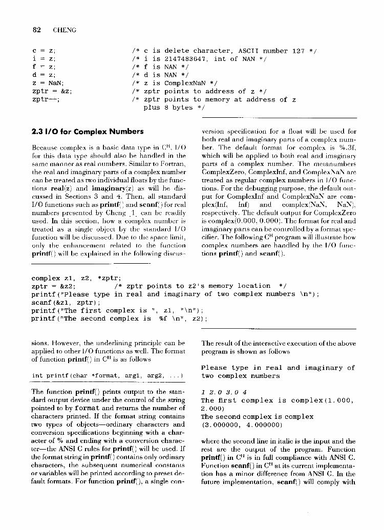
z NaN; I* z is ComplexNaN *I zptr = &z; zptr++;

I* zptr points to address of z *I I* zptr points to memory at address of z

plus 8 bytes

2.31/0 for Complex Numbers

Because complex is a basic data type in CH, II 0 for this data type should also be handled in the same manner as real numbers. Similar to Fortran, the real and imaginary parts of a complex number can be treated as two individual floats by the func­tions real(z) and imaginary(z) as will be dis­cussed in Sections 3 and 4. Then, all standard 110 functions such as printf() and scanf() for real numbers presented by Cheng [ 1] can be readily used. In this section, how a complex number is treated as a single object by the standard 1/0 function will be discussed. Due to the space limit, only the enhancement related to the function printf() will be explained in the following discus-

complex z1, z2, *zptr;

*I

version specification for a float will be used for both real and imaginary parts of a complex num­ber. The default format for complex is %.3f, which will be applied to both real and imaginary parts of a complex number. The metanumbers ComplexZero, Complexlnf, and ComplexNaN are treated as regular complex numbers in 1/0 func­tions. For the debugging purpose, the default out­put for Complexlnf and ComplexNaN are com­plex(lnf, lnf) and complex(NaN, l'\aN), respectively. The default output for ComplexZero is complex(O.OOO, 0.000). The format for real and imaginary parts can be controlled by a format spe­cifier. The following CH program will illustrate how complex numbers are handled by the 1/0 func­tions printf() and scanf().

zptr = &z2; I* zptr points to z2's memory location *I printf("Please type in real and imaginary of two complex numbers \n"); scanf(&z1, zptr); printf ("The first complex is ", z1, "\n") ; printf ("The second complex is %f \n", z2) ;

sions. However, the underlining principle can be applied to other II 0 functions as well. The format of function printf() in CH is as follows

int printf(char *format, argl, arg2, ... )

The function printf() prints output to the stan­dard output device under the control of the string pointed to by format and returns the number of characters printed. If the format string contains two types of objects-ordinary characters and conversion specifications beginning with a char­acter of % and ending with a conversion charac­ter-the ANSI C rules for printf() will be used. If the format string in printf() contains only ordinary characters, the subsequent numerical constants or variables will be printed according to preset de­fault formats. For function printf(), a single con-

The result of the interactive execution of the above program is shown as follows

Please type in real and imaginary of two complex numbers

1 2.0 3. 0 4 The first complex is complex(1.000, 2. 000) The second complex is complex (3.000000, 4.000000)

where the second line in italic is the input and the rest are the output of the program. Function printf() in CH is in full compliance with ANSI C. Function scanf() in CHat its current implementa­tion has a minor difference from ANSI C. In the future implementation, scanf() will comply with

CO~IPLEX :'\u~IBERS I'\ C11 PROGRA:\1""1Il"G LA:\GLAGE 83

ANSI C; besides. it will accept the input constants such as Complexlnf, Conmplexl\"al\", complex(2, 3.8F), etc.

3 COMPLEX OPERATIONS

The arithmetic and relational operations for com­plex numbers are treated in the same manner as those for real numbers in CH. This section will discuss how these operations are defined and handled by CH.

3.1 Complex Operations With Regular Complex Numbers

The negation of a complex number, and arith­metic and comparison operations for two complex numbers are defined in Table 1, where the com­plex numbers z, z 1 , and z2 are defined as x + iy, x1 + iy1, and x2 + iy2, respectively.

The negation of a complex number will change the sign of both real and imaginary parts of the complex number. The addition of two complex numbers will add real and imaginary components of two complex numbers, separately. The sub­traction of two complex numbers will subtract real and imaginary parts of the second complex num­ber from real and imaginary of the first complex number, respectively. Treating the imaginary number i as a complex number of complex(O, 1 ), the multiplication and division for two complex numbers are defined in Table 1. For binary oper­ations with real and complex operands, the regu­lar real operand will be cast into a complex before the operation. Complex numbers are not ordered, one cannot compare whether one complex num­ber is larger or smaller than the other. But two complex numbers can be tested whether they are equal or not. Two complex numbers are equal to each other if both real and imaginary parts of two

complex numbers are equal to each other, sepa­rately. If real or imaginary parts of two complex numbers are not equal to each other, two complex numbers are not equal.

3.2 Complex Operations With Complex Metanumbers

In the above definitions of complex operations, we assume that all operands are regular complex numbers. The real and imaginary parts of a com­plex number are then treated as two regular float­ing-point floats. If the values of operands involve complex metanumbers, the definitions defined in Table 1 may not be valid. For example, Complex­In£ is represented internally as complex(lnL lnf). According to the complex addition definition de­fined in Table 1 and the addition rule for real numbers discussed by Cheng [ 1], the result of ad­clition of two Complexlnfs would be complex(lnf, lnf). But, addition of two complex infinities is mathematically indeterminate. Therefore, the results for arithmetic and relational operations with both regular complex numbers and complex metanumbers are defined in Tables 2 to 7.

From a programmer's point of view, values of complex(±O.O, ±0.0) are the same as com­plex(O.O, 0.0) or ComplexZero when they are used as operands or arguments in CH. In the fol­lowing discussions, the positive zero 0.0 and the negative zero -0.0 for real and imaginary compo­nents of a complex number are considered the same. Therefore, although the negation of com­plex(O.O, 0.0) returns complex(-0.0, -0.0), the result listed in Table 2 is complex(O.O, 0.0). Nega­tion of a complex infinity is still a complex infinity. Of course, negation of a complex not-a-number is ComplexNaN.

For binary operations in Tables 3 to 5, if any one of the operands is Comple:xl\'aN, the result is ComplexNaN. If one of two operands is Complex-

Table 1. The Complex Operations

Definition CH Syntax CH Semantics

Negation -z -x- iy Addition zl + z2 (x1 + xz) + i(Yt + Yz) Subtraction zl + z2 (x1 - xz) + i(y1 + Yz) Multiplication zl * z2 (x1 * x2 - Y1 * Y2) + i(y1 * x2 + Xt * Y2)

Division zl I z2 Xt * X2 + Yt * Y2 . Yt * X2 - Xt * Y2 2 _rl +1 2 _rl X2 + 2 X2 + 2

Equal zl == z2 Xt == x2 andy1 == Yz Not equal zl != z2 x1!= or Yt != Y2

84 CHE~G

Table 2. Negation Results

Negation-

Operand Result

complex(O.O, 0.0) complex(O.O, 0.0)

z -z

Complexlnf Complexlnf

ComplexNa~

Complex~ aN

Table 3. Addition and Subtraction Results

Addition and Subtraction ±

Right Operand

Left Operand complex(O.O, 0.0) z2 Complexlnf Complex~ a]\'

complex(O.O, 0.0) complex(O.O, 0.0) ±z2 Complexlnf Complex:\ a:\ zl z1 z1 ± z2 Complexlnf Complex:t\'a'\1 Complexlnf Complexlnf Complexlnf Complex:\ a:\ Complex]\' a'\/ ComplexNa~ Complex;\' al\' Complex~ aN Complex:\ a-"' Complex:\ a:'\

Table 4. Multiplication Results

Multiplication * Right Operand

Left Operand complex(O.O, 0.0) z2 Complexlnf Complex:'\ a]\

complex(O.O, 0.0) zl Complexlnf ComplexNal\'

Table 5. Division Results

complex(O.O. 0.0) complex(O.O, 0.0)

Complex'\ial\' Complex~ a]\

complex(O.O. 0.0) z1*z2

Complexlnf Complex.'\: a]\

Division +

Complex:\ a:\ Complexlnf Complexlnf

Complex:\ a:\

Complex~ a]\' Complex:\ a:\ Complex!'\ a~ Complexl\'a:\

Right Operand

Left Operand

complex(O.O, 0.0) zl Complexlnf Complex!\. a'\/

complex(O.O, 0.0)

complexl'\a'>J Complexlnf Complexlnf

Complex:\ a:\

z2

complexiO.O. 0.0; z1/z2

Complexlnf Complex:\ a.:\

Table 6. Equal Comparison Results

Equal Comparison = =

Complexlnf

complex(O.O. 0.0) complex(O.O. 0.0)

Complex~'\ a:\ CmnpiPx.:\a:\

Right Operand

Left Operand complex(O.O. 0.0) z2 Cornplexlnf Complex:\ a:\

complex(O.O, 0.0) 1 () 0 0 zl 0 z1 == z2 () ()

Complexlnf 0 0 1 0 Complex]\ a:\ 0 0 ()

Complex]\ a:\

Complex!\: a:\ Complex~ a:\ Complex~ a:\ ComplE'x."\a.:\

COMPLEX ~C\1BERS I~ C11 PROGRAMMl~G L\:\GCAGE 85

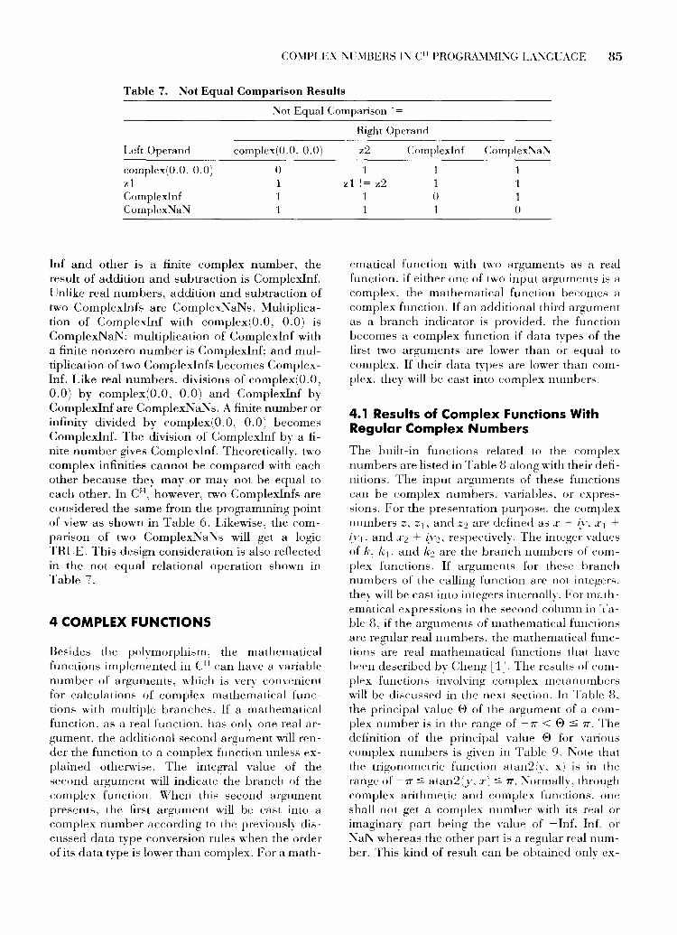
Table 7. Not Equal Comparison Results

:'1/ot Equal Comparison ~ =

Left Operand complex(O.O, 0.0)

complex(O.O, 0.0) 0 z1 1 Complexlnf 1 ComplexNal\i 1

lnf and other is a finite complex number, the result of addition and subtraction is Complexlnf. Unlike real numbers, addition and subtraction of two Complexlnfs are ComplexNaNs. :\1ultiplica­tion of Complexlnf with complex(O.O, 0.0) is ComplexNaN; multiplication of Complexlnf with a finite nonzero number is Complexlnf; and mul­tiplication of two Complexlnfs becomes Complex­In£. Like real numbers, divisions of complex(O.O, 0.0) by complex(O.O, 0.0) and Complexlnf by Complexlnf are ComplexNaNs. A finite number or infinity divided by complex(O.O, 0.0) becomes Complexlnf. The division of Complexlnf by a fi­nite number gives Complexlnf. Theoretically, two complex infinities cannot be compared with each other because they may or may not be equal to each other. InCH, however, two Complexlnfs are considered the same from the programming point of view as shown in Table 6. Likewise, the com­parison of two Complexl\"al\s will get a logic TRUE. This design consideration is also reflected in the not equal relational operation shown in Table 7.

4 COMPLEX FUNCTIONS

Besides the polymorphism. the mathematical functions implemented in CH can have a variable number of arguments. which is very convenient for calculations of complex mathematical func­tions with multiple branches. If a mathematical function. as a real function. has onlv one real ar­gument. the additional second argument will ren­der the function to a complex function unless ex­plained otherwise. The integral value of the second argument will indicate the branch of the complex function. When this second argument presents, the first argument will be cast into a complex number according to the previously dis­cussed data type conversion rules when the order of its data type is lower than complex. For a math-

Right Operand

z2 Complexlnf Complex~ a:\

1 1 1 z1 != z2 1 1

1 0 1 1 1 0

ematical function with two arguments as a real function, if either one of two input arguments is a complex. the mathematical function becomes a complex function. If an additional third argument as a branch indicator is provided. the function becomes a complex function if data types of the first two arguments are lower than or equal to

complex. If their data types are lower than com­plex. they will be cast into complex numbers.

4.1 Results of Complex Functions With Regular Complex Numbers

The built-in functions related to the complex numbers are listed in Table 8 along with their defi­nitions. The input arguments of these functions can be complex numbers. variables, or expres­sions. For the presentation purpose. the complex numbers z, z 1 , and z~ are defined as x + (v. x· 1 + iy1. and x 2 + iy2. respectively. The integer values of k, k 1 , and k2 are the branch numbers of com­plex functions. If arguments for these branch numbers of the calling function are not integers. they will be cast into integers internally. Form& th­ematical expressions in the second column in 'fa­ble 8. if the arguments of mathematical functions are regular real numbers. the mathematical func­tions are real mathematical function:,; that have been described by Cheng [1!. The results of com­plex functions involving complex metanumbers will be discussed in the next section. ln Table 8. the principal value 0 of the argument of a com­plex number is in the range of -rr < 0 :S rr. The definition of the principal value 0 for various complex numbers is given in Table 9. Note that the trigonometric function atan2(y, x) is in the range of -rr :S atan2(J·. x) :S rr. ~ormally. through complex arithmetic and complex functions. one shall not get a complex number with its real or imaginary part being the value of -lnf. Inf. or ]\;al\ whereas the other part is a regular real num­ber. This kind of result can be obtained onlv ex-

Table 8. The Syntax and Semantics of Built-in Complex Functions

C11 Syntax

sizeof(z) abs(z) real(z) imaginary(z) complex(x, y) conjugate (z) polar(z) polar(r, theta)

sqrt(z)

sqrt(z, k)

exp(z) log(z) log(z, k)

log10(z)

log10(z, k)

pow(z1, z2) pow(zJ, z2, k) ceil(z) floor(z)

fmod(z1, z2)

modf(z1, &z2) frexp(zL &z2) ldexp(z1, z2) sin(z) cos(z)

tan(z)

asin(z) asin(z, k) asin(z, k1, k2) acos(z) acos(z, k) acos(z, k1, k2)

atan(z)

atan(z, k)

atan2(z1, z2)

atan2(z1, z2, k)

sinh(z) cosh(z)

tanh(z)

asinh(z) asinh(z, k) asinh(z, k1, k2) acosh(z) acosh(z, k) acosh(z, k1, k2)

atanh(z)

atanh(z, k)

Cl1 Semantics

y X+ iy X- iy sqrt(x2 + rl + i0: 0 = atan2(y, x) r cos(theta) + ir sin(theta)

' ( 2 2Jl( 0 . . 0) 0 2' sqrt\sqrt x + .Y cos2 + t sm 2 : • = atan 1,y,

' ( 2 .2Jl( 0 + 2k1r 0 + 2k1r) 0 sqrt1,sqrt x + .Y cos 2

+ i sin 2

: •

ex( cosy + i sin y) log(Vx2 + rl + i0: 0 = atan2 x) log(V x 2 + r) + i(0 + 2k1r); 0 = atan2Cr. x)

~ log(10) log(z, k) log (10) ZJz2 = ez2lnzt = exp[z2 * log(zJ)] z1z2 = ez2lnz, = exp[z2 * log(zJ, k)] ceil(x) + i ceil(y) floor(x) + i floor(y)

z: ZJ = k + ~. k ;, () Z2 Z2'

modf(x 1 , &x2) + i modf(y2, &y2) frexp(x!, &x2) + i frexp(y1, &y2) ldexp(x!, x2) + i ldexp(y!, Y2) sin xcosh y + i cos x sinh y cos x cosh y - i sin x sinh y Sill Z

cos z -i log[iz + sqrt(1 - z2)] -i log[iz + sqrt(1 - z2, k)] -i log[iz + sqrt(1 - z2 , kJ), k2]

-i log[z + isqrt(1 - z2)] -i log[z + isqrt(1 - z2, k)] -i log[z + isqrt(1 - z2, kJ), k2]

1 (1 + iz) 2i log 1 - iz

1 (1 + iz ) 2i log 1 - iz' k

1 I ( 1 + iz1/z2 2i og 1 - iz1/z2

1 (1 + iz1/z2 ) -2 · log 1 · 1 I · k l - lZ Z2' sinh x cos y + i cosh x sin y cosh x cos y + i sinh x sin y sinh x cos y + i cosh x sin y cosh x cos y + i sinh x sin y log[z + sqrt(z2 + 1)] log[z + sqrt(z2 + 1, k)] log[z + sqrt(z2 + 1, kJ), k2] log[ z + sqrt(z + 1 )sqrt(z - 1)] log[z + sqrt(z + 1, k)sqrt(z- L k): log[ z + sqrt(z + 1, kJ)sqrt(z - 1, kJ), k2]

1. log (1 + z) 2 1 - z

1 (1 + z ) 2log 1 - z' k

atan2 (y. x)

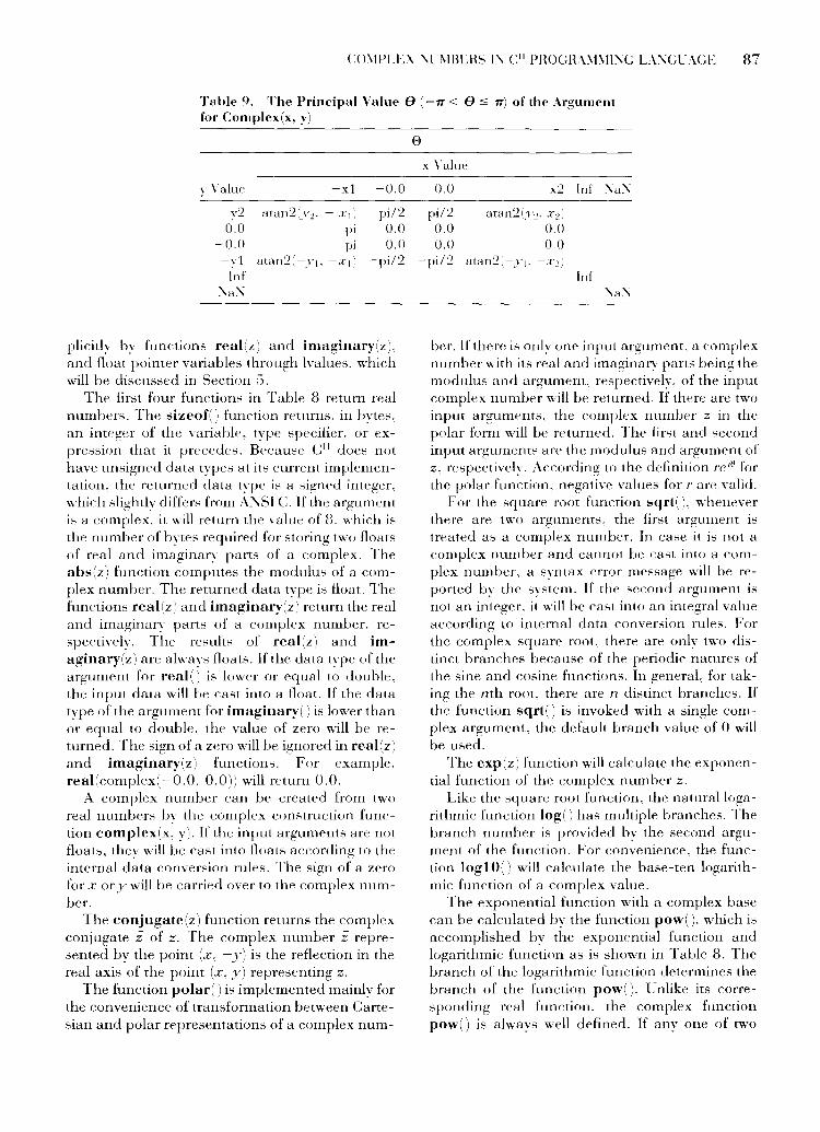
CO\fPLE\. :\C\113ERS 1.\ <: 11 PROGRA\1\fl:\G L:\\GL\GE 87

Table 9. The Principal Value f) ( -1T < f):::; 1r) of the Ar!!:ument for Complex(x. y)

y Value

v2 0.0

-0.0 -v1

Tnf \a\

atan2(.n.

atan2(-yJ.

-x1 -0.0

- XJJ pi/2 pi 0.0 pi 0.0

-x 1 \~ -pi/2

plicitly by functions real(z) and imaginary(z). and float pointer variables throu~d1 !values. which will be discussed in Section 5.

The first four functions in Table 8 return real numbers. The sizeof() function returns. in bytes, an integer of the Yariable. type specifier. or ex­pression that it precedes. Because C11 does not have unsigned data types at its current implemen­tation. the returned data type is a signed integer, which slightly differs from A:'\SI C. lf the argument is a complex. it will return the value of 8. which is the number of bytes required for storing two floats of real and imaginary parts of a complex. The abs(z) function computes the modulus of a com­plex number. The returned data type is float. The functions real(z) and imaginary(z) return the real and imaginary parts of a complex number. re­spectively. The results of real(z) and im­aginary(z) are always floats. If the data type of the argument for real() is lower or equal to double, the input data will be cast into a float. If the data type of the argument for imaginary() is lower than or equal to double, the value of zero will be re­turned. The sign of a zero will be ignored in real(z) and imaginary(z) functions. For example. real(complex(-0.0. 0.0)) will return 0.0.

A complex number can be created from two real numbers by the complex construction func­tion complex(x, y). If the input arguments are not floats, they will be cast into floats according to the internal data conversion rules. The sign of a zero for x or y will be carried over to the complex num­ber.

The conjugate(z) function returns the complex conjugate z of z. The complex number z repre­sented by the point (x, -y) is the reflection in the real axis of the point (x, y) representing z.

The function polar() is implemented mainly for the convenience of transformation between Carte­sian and polar representations of a complex num-

0

x \'alu(;

0.0 x2 lnf \a\

pi/2 atan2 (.1·2· .1'2 /

0.0 0.0 0.0 0.0

-pi/2 atan2~-.r 1 • -.r:.z

lnf

her. If there is only one input argument. a complex number with its real and imaginary parts being the modulus and argument. respectively. of the input complex number will be returned. If there are two input arguments. the complex number z in the polar form will be returned. The first and second input arguments are the modulus and argument of z. respectively. According to the definition re 10 for the polar function. negative values for rare valid.

For the square root function sqrt( ), whenever there are two arguments. the first argument is treated as a complex number. In case it is not a complex number and cannot be cast into a com­plex number. a syntax error message will be re­ported by the system. If the second argument is not an integer. it will be cast into an integral value according to internal data conversion rules. For the complex square root. there are only two dis­tinct branches because of the periodic natures of the sine and cosine functions. In general. for tak­ing the nth root. there are n distinct branches. If the function sqrt() is invoked with a single com­plex argument. the default branch value of 0 will be used.

The exp (z) function will calculate the exponen­tial function of the complex number z.

Like the square root function. the natural loga­rithmic function log() has multiple branches. The branch number is provided by the second argu­ment of the function. For convenience. the func­tion log1 0() will calculate the base-ten logarith­mic function of a complex value.

The exponential function with a complex base can be calculated by the function pow(). which is accomplished by the exponential function and logarithmic function as is shown in Table 8. The branch of the logarithmic function determines the branch of the function pow(). Cnlike its corre­sponding real function. the complex function pow() is always well defined. If any one of two

88 CHENG

arguments of pow(z1, z2) is complex, the result is complex, which is obtained by the principal branch of the expression exp(z2*log(z1)). The result of the expression yx equals the real part of the expression pow(complex(y, 0.0), complex(x, 0.0)) with its imaginary part being zero. For the function pow(z1, z2, k), z1 and z2 can be any data type lower than or equal to complex, and k is an integer. Whenever there are three arguments for the function pow(), the first and second argu­ments are treated as complex numbers. If z2 is an integer, all branches will have the same result; thus, the solution is unique.

For functions ceil(z), ftoor(z), and ldexp(zl. z2), the real and imaginary parts are treated as if they were two separate real functions. The func­tions modf(z1, &z2) and frexp(z1, &z2) are han­dled in the same manner. For these two functions. when the data type of the first arguments is com­plex, the data type of the second argument must be a pointer to complex. The fmod(z1, z2) func­tion computes the complex remainder of z1/z2.

The complex trigonometric functions sin(z ). cos(z), and tan(z) and complex hyperbolic func­tions sinh(z), cosh(z), and tanh(z) have unique values. However, the complex inverse trigonomet­ric functions asin(z), acos(z) and atan(z) and complex inverse hyperbolic functions asinh(z). acosh(z), and atanh(z) have multiple branches for a given input complex value. The second argu­ment of these inverse functions indicates the branch number. For functions asin(), acos( ), asinh(), and acosh( ), the second and third argu­ments specify the branches of the related square root and logarithmic functions. respectively. The function atan2() is implemented similar to the function atan( ).

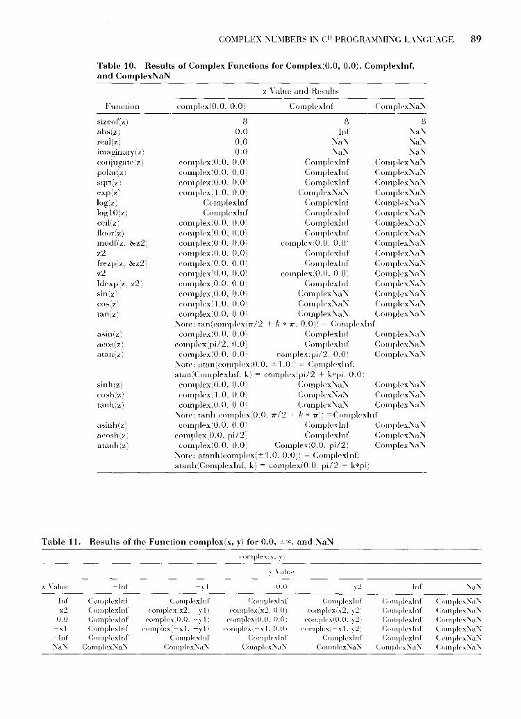
4.2 Results of Complex Functions With Complex Metanumbers

Like complex arithmetic operations. the definition for regular complex functions may not be valid when the input arguments are complex metanum­bers. The results of the built-in complex functions with complex metanumbers as their input argu­ments are given in Table 10. In Table 10. com­plex(±O.O, ±0.0) inCH is treated as complex(O.O, 0.0). \\rhen the input argument of a function is Complex[\al'\, the returned result is always Com­plexl'\a~ except for the function sizeof(). As shown in Figure 2, a complex infinity is different from the real infinites of ±x. \\'hen either the real or imaginary part of a complex value is outside the

range of the representable floating-point number, it becomes Complexlnf. Therefore, the absolute value of Complexlnf is a real number of Inf. The real and imaginary parts of Complexlnf are NaN. However, the conjugate of Complexlnf is still a complex infinity. The result polar(complex(O.O, 0.0)) is defined'as complex(O.O, 0.0) because the principal value E> for complex(O.O, 0.0) equals 0.0 as defined in Table 9. The result of polar(Com­plexlnf) is defined as complex(Inf, Inf). Therefore, if z equals complex(O.O, 0.0) or Complexlnf, the equality of z = polar(real(polar(z) ), imaginary(po­lar(z))) will still be satisfied. Like a real function, the square root of Complexlnf is Complexlnf.

As a real function, exp(Inf) = Inf whereas exp(-lnf) = 0.0. However, both values of ±Inf become Complexlnf if they are cast into complex numbers. Therefore, the complex exponential function exp(z) is Complexl'\ai\ when the input argument is Complexlnf. The complex logarith­mic function log(z) with the input argument of complex(O.O, 0.0) or Complexlnfwill return Com­plexlnf. \Vith complex metanumbers as their in­put arguments, the real and imaginary parts of functions ceil(z), ftoor(z). and ldexp(zl. z2) are handled equivalent to two individual real func­tions. Like real functions. the complex trigono­metric functions sin(z), cos(z), and tan(z) are un­defined when the input arguments are Complexlnfs. The irrational number 1T is not rep­resentable in a computer program. If we had the value of 1T. the expression of tan(k7T + 7T/2) would return Complexlnf. Cnlike real functions, the complex inverse trigonometric functions asin(z) and acos(z) return Complexlnfs when the input arguments are Complexlnfs. As an inverse func­tion oftan(z), the function atan(z, k) has different branches when the first input value is Complexlnf. According to the definition, atan(±i) equals Com­plexlnf. The results of the complex hyperbolic functions sinh(z), cosh(z). and tanh(z). and complex inverse hyperbolic function" asinh ( z). acosh(z). and atanh(z) are implemented :-iimilar to those of complex trigonometric functions and complex inverse trigonometric functions.

The results of the complex construction func­tion complex(x, y) are given in Table 11. For con­structing a complex number. if either its real or imaginary part is 1'\a:\" .. the result is a complex i\ot-a-1'\umber. Likewise. if either one is a value of ±x, the result is Complexlnf. For the function polar(r, theta) shown in Table 12, when the mod­ulus is infinitely large, the resultant complex num­ber is Complexlnf even if the provided argument

CO.\IPLEX :\L.\IBERS 1:\ C11 PROGRA.\1.\11:\G LA:\GL\GE 89

Table 10. Results of Complex Functions for Complex(O.O, 0.0), Complexlnf, and ComplexNaN

Function

sizeof(z) abs(z) real(z) irnal!inary(z) conjugate(z) polar(z) sqrt(z j exp(z) log(z) log10(z) ccil(z) floor(z) rnodf(z. &z2) z2 frezp(z. &z2) z2 ldexp(z. z2) sin(z) cos(z) tan(z)

asin(z) acos(z) atan(z)

sinh(z) cosh(z: tanh(z)

asinh(z) acosh(z) atanh(z)

complex(O.O. O.Oj

8 0.0 0.0 0.0

z \. alue and Results

Complexlnf

8 lnf

:\a:\ :\a:\

Complex:\ a:\

8 :\a:\ .'\a:\ :\a:\

cornplex(O.O. 0.0: Complexlnf Complex:\a:\ complex(O.O. 0.0) Complexlnf Complex:\a:\· complex(O.O. O.Oj Complexlnf Complex:\a:\ complex(1.0. O.Oj Complex:\a:\ Complex:\a:\

Cornplexlnf Complexlnf Complt>x:\a:\ Complexlnf Complexlnf Complex:\a:\

cmnplex(O.O. 0.0; Complexlnf Complex:\a:\ complex(O.O. 0.0) Complexlnf C:ornplex:\a:\ complex(O.O. 0.0) complex'O.O. 0.0' Complex:\a:\ complex(O.O. 0.0) Cornplexlnf Complt>x:\a:\ complex',(). 0. 0. 0) Complexlnf Complex:\ a:\ complex(O.O. 0.0) complex~O.O. 0.0: Complex:\a:\ complex(O. 0. 0. 0) C:omplexlnf Cmnplex.'\a:\ complex(O.O. 0.0) Cornplex:\a:\ Complex:\a:\ complex(1.0. 0.0) Complex:\a:\ Complex:\a:\ complex(O. 0. 0. 0'! Complex:\ a:\ Complex:\ a:\·

:\ote: tan(cornplt>x(7T/2 + k * 1r. O.or = Complexlnf complex(O.O. O.(J:I Complexlnf Cornplex:\a:\

complex~pi/2. 0.0) Complexlnf Complex:\a:\ complex1:0.0. 0.0) complex:pi/2. 0.()1 Complex:\a:\

:\ott>: atanlcomplex(O.O. ±1.0il = Cornplexlnf: atan(Complexlnf. k) = complex(pi/2 + bpi. 0.0:

complex(O.O. (J.O) Cornplex:\a:\ C:omplex:\a:\ complexi1.0. 0.0; Complex:\a:\ Cornplex:\a:\ complex(O.O. 0.()! Complex:\a:\ Complex:\a:\

:\ote: tanh(complex(O.O. 7T/2 + k * 77)) =Complexlnf cmnplex(O.O. 0.0) Complexlnf Complex:\a:\

cornplex\0.0. pi/2' Complexlnf Comph·x:\a'>i complex(O.O, O.Oj Complex(O.O. pi/2) Complex:\a:\

"'otc: atanh(complex(±1.0. 0.0)) = Complcxlnf: atanh(C:omplcxlnf. k) = complex(O.O. pi/2 + k*pi)

Table 11. Results of the Function complex(x, y) for 0.0. ±oc, and "iaN

x Yalue

Inf x:2

0.0 -x1 -lnf '\a'\

-lnf

Compkxlnf Cornplexlnf Complexlnf ComplPxinf Complexlnf

Complex:'\ a'\

-yj

CornpiPxlnf

''omp1Px'x:2. -d ·' complcx(O.O. -v1

complex. -xl. -v1'!

Complexlnf Complex:\a'i

\ \'ah"·

0.0

C:mnplexlnf complex·'x:2. 0.0;

compil'x10.0. 0.0 eompiPx -x1. 0.0.

Compkxlnf Complex'\ a:\

CompiPxlnf complcx.'x:2. v:2,

complex10.0. Y:2: complex·- x 1. ,.:2'·

Cornplexlnf CompiPx'\a'\

lnf

Cornplexlnf Cornplexlnf <:ompiPxlnf Complexlnf Complt·xlnf

Cmnplex'\a'\

Cornplcx'\a:\ CompiPx'\a:\' Complex'\ a:\ ComplPx'\a'\ Complex'\a:\ Complex'\a'\

90 CHE:'\iG

Table 12. Results of the Function polar(r, theta) for 0.0, ±00. and !\'aN

polarlr. tlwta \

Theta Value

r Value ~Jnf ~theta 1 0.0 theta:2

lnf Complcxlnf Cornplexlnf Cornplexlnf Cmnplexlnf r2 Complex:\ a'-/ polm··:r2. ~theta1; comp1Px(r2. 0.()', polarlr:2. tbeta:z:,

0.0 Complex:\ a!\ cmnpltex!O.O. 0.0) complex(O.O. 0.0' complex'O.O. 0.0' ~rl Complex"! a!\ polan'~rl. ~thetal) complexi~r1. 0.0' polar(~r1. theta:!., ~Inf Complexlnf Complexlnf Complexlnf Curnplexlnf "iaN Complcxl\'ai\ Complex!\ a:\ Compltex"'a:\ Complex:\a'-1

lnf

Cmnplexlnf Compkxl\'a:\ Complt>x:\a:\ Complex:\a:\

CnntplPxlnf ( :omplex:\a:\

Complex:\a:\ (:omplex:\a:\ Complex:\ a:\ Complex:\a:\ Complex:\a:\ Complex:\ a:\'

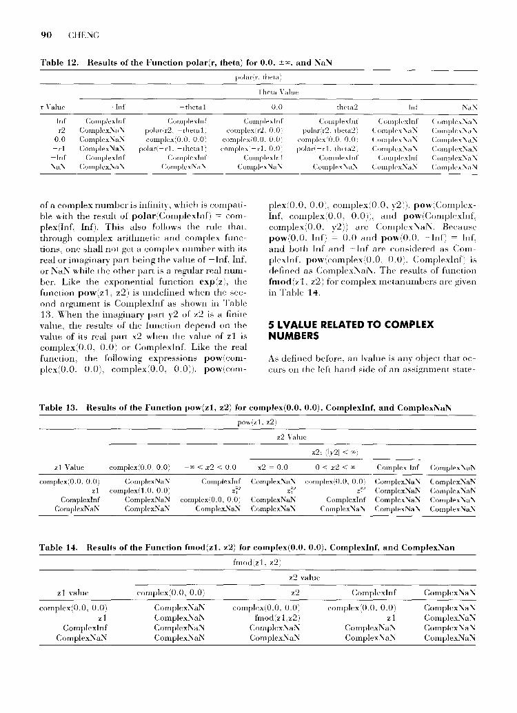
of a complex number is infinity, which is compati­ble with the result of polar(Complexlnf) = com­plex(lnf, Inf). This also follows the rule that .. through complex arithmetic and complex func­tions, one shall not get a complex number with its real or imaginary part being the value of -lnL InL or .Ka.K while the other part is a regular real num­ber. Like the exponential function exp(z), the function pow(z1, z2) is undefined when the sec­ond argument is Complexlnf as shown in Table 13. When the imaginary part y2 of z2 is a finite value, the results of the function depend on the value of its real part x2 when the value of z1 is complex(O.O. 0.0) or Complexlnf. Like the real function, the following expressions pow(com­plex(O.O, 0.0), complex(O.O, 0.0)). pow(com-

plex(O.O. 0.0). complex(O.O. y2)). pow(Complex­lnf, complex(O.O. 0.0)). and pow(ComplexlnL complex(O.O, y2)) are Complex.Ka.i\'. Because pow(O.O .. lnf) = 0.0 and pow(O.O, -lnf) = lnf, and both lnf and - lnf are considered as Com­plexlnf. pow(complex(O.O. 0.0). Complexlnfl is defined as Complex_I\Ja.i\'. The results of function fmod(zL z2) for complex metanumbers are given in Table 14.

5 LVALUE RELATED TO COMPLEX NUMBERS

As defined before, an lvalue is any object that oc­curs on the left hand side of an assi§!nment state-

Table 13. Results of the Function pow(z1, z2) for complex(O.O, 0.0), Complexlnf, and ComplexNaN

z1 Value

complex(O.O, 0.0) z1

Cornplexlnf ComplexNaN

complex(O.O, 0.0)

ComplexNal\ complex(1.0, 0.0)

Complexl\'aN Complex!'iaN

pow(zl. z2)

z2 Value

~oo < x2 < 0.0

Complexlnf z~2

complex(O.O. 0.0) CompleL:\a!\

x2 = 0.0

Complex:\a"J z~:?

ComplexNaN Complex.c'lal\

0 < x2 <co

complex(O.O. 0.0) "' z,·

Cumplexlnf Complex:\aJ'Ii

Complex Inf

Complex:\! aN ComplexNal\' ComplexNa"' ComplexNal\'

Complex:'~/ aN

ComplexNa)'l; ComplexNal\' Complex:\ a:\ ComplexNaN

Table 14. Results of the Function fmod(z1, z2) for complex(O.O, 0.0), Complexlnf, and ComplexNan

z1 value

complex(O.O, 0.0) z1

Complexlnf Complex!\' a:'\

complex(O.O, 0.0)

Com plex:'li' a!\' Complex!\' aN Complex!\ a~ Complex."\ aN

fmod(zL z2)

z2 value

z2

complex(O.O. 0.0) fmod(zLz2)

Complex!\' a:\ Complex~ a'\

Complexlnf

cornplex(O.O. 0.0) z1

Complex!\' a~ Complex:\' a:\'

Complex!\' a:\'

Complex:\' a:\' Complex~ a~

Complex~ a!\' ComplexNa:\'

CO.\IPLEX :\l.\IHERS 1:\ Ci 1 PROCR\.\1.\li:\G L\:\GL\GE 91

Table 15. The Valid lvalues Related to Complex Numbers

Case

1 2 .3

4

.\1eaning of lvalue

Simple variable An element of a complex array Complex pointer variable

Address pointed to by a complex variable An element of a complex pointer array

6 Address pointed to by an element of a complex

7

8

9

pointer array Real part of a complex variable Real part of a complex variable Real part of a complex variable Imaginary part of a complex variable Imaginary part of a complex variable Imaginary part of a complex variable Imaginary part of a complex variable Float pointer variable

Pointer to real part of a complex variable Pointer to imaginary part of a complex variable

ment. The valid !values related to complex num­bers are listed in Table 15. The assignment operations+=.-= .. *=,!=. as well as increment operation + + and decrement operation -- de­scribed by Cheng [1: can be applied to all these !values. Besides the simple variable in case 1. an element of a complex array can be an !value which is case 2 in Table 1.3. In case 3. pointer to com­plex is used as an !value to get the memory or to point to a memory of a complex object. In case 4. the memory pointed to by the pointer zptr is as­signed the value of the expression on the right hand side of an assignment statement. In addition to a single pointer variable. one can have an array of complex pointers. Cases 5 and 6 show how an element of a complex pointer array is used to ac­cess the memory. The function real () cannot only be used as an rvalue or an operand. it can also be used as an !value to access the memory of its argu­ment. In case 7, the argument of real() must be a complex variable. or an address pointed to by a complex pointer or pointer expression. A constant complex number or expression can be used as an input argument of the function real () only when it is an rvalue or an operand. In case 8. the imagi­nary part of a complex is accessed by the function imaginary() in the same manner as the function real(). Because a complex number occupies two floats internally, this memory storage can be ac-

Example

z =complex (1. 0, 2); zarray[i] = complex(l. 0, 2)+ Complexinf; zptr = malloc (sizeof (complex) * 3; zptr = &z; *zptr =complex (1. 0, 2) + z; zarrayptr [i] = malloc (sizeof (complex) * 3; zarrayptr [i] = &z;

*zarrayptr[i] =complex(l.O, 2); real (z) = 3. 4; real (*zptr) = 3. 4; real(*(zptr+l)) =3.4; imaginary (zl =complex (1. 0, 2); imaginary (*zptr) = 3. 4; imaginary(*(zptr+l)) = 3. 4; imaginary (*zarrayptr [ i]) = 3. 4; fptr = &z; fptr = zptr; *fptr = 1. 0; *(fptr+l) =2.0;

cessed not only by the functions real() and imag­inary(). but also by a pointer to float as is shown in case 9 where the variable fptr is a pointer to float. For cases 7-9 .. a real number. including ±0.0. ±lnf. and ::\al\'. on the right hand side will be assigned to an !value formally without filtering. Therefore, abnormal complex numbers such as complex(lnf.. l\'a~). complex(lnf. 0.0). etc. may be created. For example. two CH commands real(z) = :\'al\' and imaginary(z) = lnf make z equal to complex(l\an, lnf): and rcal(z) = -0.0 and imaginary(z) = l\'Zero gives z the value of complex(-0.0. -0.0).

6 CREATION OF USER'S COMPLEX FUNCTIONS

Cser's complex functions inCH can be created in the spirit of A~Sl C. which will be demonstrated by the computation of the gamma function f(z). f(z) can be defined by the integral as follows:

(3)

One of the approximation formulas for the func­tion f(z) derived by Lanczos [18] is as follows:

92 CHE~G

r() ( 4 5) () - 1 +4-' ~ ;o- ( O 76.18009173 z = z + . z- ,oe- z '"1 V 27T 1. + z + 1

86.50532033 z + 2

24.01409822 + -----=--­z+3

1.231739516 ------+ z+4

0.120858003e-2

z+5 0.536382e-> + e)

z+6 (4)

with the error smaller than lei < 2 * 10-10 . The above formula is valid for the complex gamma function in the half complex plane of real(z) > 0. To avoid the overflow, log[f(z)] rather than f(z) is usually computed. For example, the logarithm of the above approximation formula for the gamma function with a float argument has been pro­grammed by Press et al. [19] in C. The complex version of the logarithm of the gamma function can be easily programmed inCH as follows.

complex gammalog(complex z) {

complex zz, sum;

1. Follow conventional mathematics; define values for all operations and functions over the entire domain.

2. Preserve ANSI C and Fortran styles. The in­terpretation will follow C whenever there is a syntax conflict.

3. Make language easy to use, 4. Make language easy to implement.

These principles are reflected in many features of the CH programming language. Some features like

sum= 1.0 + 76.18009173/(z+1) - 86.50532033/(z+2) + 24.01409822/(z+3) -1.231739516/(z+4) + 0.120858003e-2/(z+5) -0.536382e-5/(z+6);

zz = (z-0. 5) *log (z+4. 5) - (z+4. 5) + log (sqrt (2*PI) *sum); return zz;

}

Csing the above-programmed external gamma function, the commands of

printf("gammalog(-2) = %f \n", gammalog(-2)); printf("gammalog(complex(1,2)) = %f \n", gammalog(complex(1,2)); printf("gammalog(2) = %f \n", gammalog(2));

will produce the following output.

gammalog(-2) = complex(Inf,Inf) gammalog(complex(1,2)) = complex(-2.164028,0. 663057) gammalog(2) = complex(-0.536407,0. 000000)

Note that the gamma function gets Complexlnf at the singular point -2. For a real argument as in gammalog(2), the complex gamma function re­turns a complex number with an identically imagi­nary zero.

7 RATIONALE BEHIND CH

This section provides rationales for some of the scientific programming features of CH. The follow­ing philosophies guided me through the design and implementation of language features pre­sented in this paper and the companion paper [ 1].

polymorphism of built-in functions and optional arguments for multiple-valued complex functions are obvious. Others. which are less obvious and even contentious. are brit>fly explained in the fol­lowing discussions.

7.1 No Unanticipated Complex Values

Cnlike conventional languages. there arP no re­served words in CH. The keyword clwngeubi!it.•· in Cl 1 makes the language very flexible. C 11 is a pro­gramming environment and can be configured at the programmer's discretion. 'Whenever appropri­ate, the decision in C' 1 will be made by the pro-

CO,\lPLEX :\l~,\lBERS I:\ C11 PROGRA,\1\tl:\C LA:\GLAGE 93

grammer, not the language implementor. This policy is also reflected in features related to com­plex numbers.

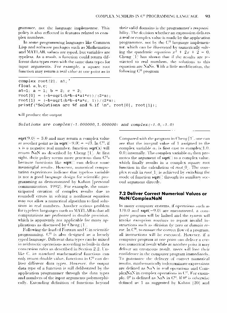
In some programming languages like Common Lisp and software packages such as }1athematica and }IA TLAB .. values are typed, but variables are typeless. As a result. a function could return dif­ferent data types even with the same data types for input arguments. For example. a square root function may return a real value at one point as in

complex root [2] , a1; • float a,b,c; a1=1; a 1; b = 2; c = 2; root[O] = (-b+sqrt(b*b-4*a1*c))/(2*a); root[1] = (-b+sqrt(b*b-4*a*c, 1))/(2*a);

their valid domains is the programmer· s responsi­bility. The decision whether an expression delivers a real or complex value is made by the application programmer. not by the CH language implemen­tor. which can be illustrated bv numericallv solv­ing the quadratic equation x 1 + 2x + 2 = 0. Cheng [1: has shown that if the results are re­stin~ted to real numbers. the solutions to this equation are !'\al'\s. ~~ith a little modification. the following CH program

printf ("Solutions are %f and %. 1f \n", root [OJ, root [1]);

will produce the output

Solutions are complex(-1. 000000,1. 000000) and complex(-1. 0, -1. 0)

sqrt(9.0) = 3.0 and may return a complex value at another point as in sqrt(-9.0) = -n. InCH. if x is a negative real number. function sqrt(x! will return l'\aN as described by Cheng [1_. At first sight. their policy seems more generous than CHs because functions like sqrt() can deliver some meaningful results. However.. numerical compu­tation experiences indicate that typele,;,; variable is not a good language design for scientific pro­gramming as demonstrated by Kahan [personal communication. 1992]. For example. the unan­ticipated creation of complex results due to roundoff errors in solving a nonlinear equation may not allow a numerical algorithm to find solu­tions in real numbers. Another serious problem for typeless languages such as ::\lATLAB is that all computations are performed in double precision. which is apparently not applicable for many ap­plications as discussed by Cheng [1:.

Following the lead ofF ortran and C in scientific programming. CH is also designed as a loosely typed language. Different data types can be mixed in arithmetic operations according to built-in data cmn·ersion rules as described in Section :2.:2. L n­like C. its standard mathematical functions can onlv return double value. functions in C 11 can de­liver different data types. However. the output data type of a function i,; still deliberated by the application programmer through the data types and numbers of the input arguments polymorphi­cally. Extending definition of functions beyond

Compared with the program in Cheng [ 1:. one can see that the integral value of 1 as:-;igned to the complex variable a 1 is first cast to complex(1.0. 0.0) internally. The complex variable a1 then pro­mote,; the argument of sqrt() to a complex value. which finally results in a complex ,;quare root function in the calculation of root[O'. The com­plex result in root r 1] i,; achieved by switchill[.( the mode of function sqrt() through it:-i auxiliary sec­ond argument dirt>ctly.

7.2 Deliver Correct Numerical Values or NaN/ComplexNaN

In rnany computer systerns .. if operations such as 1/0.0 and sqrt(-9.0) are encountered. a com­puter program will be halted and the system will invoke exception routine,; to report invalid in­structions such as diuision by zero or domain er­ror. InCH. to ensure the correct flow of a program. all instructions will be executed. However. if a computer program at one point can deliver a cor­rect numerical result while at anothPr point it may deliver an erroneous result. u:oer,; will lose their confidence in the computer program immediately. To guarantee the delivery of correct numerical results. mathematically indeterminate Pxpressions are defined as 1\'a:\ in real operations and Com­plexl\'al\' in complex operations inC"- For exam­ple. 0° is defined as :\'al\' in CH. 1f 0° is otherwise defined as 1 a,; suggested by Kahan l20] and

94 CHE:\"G

Thomas [21]. the expression of pow(x. 1/log(x)j with x 0 would deliver 1. 0: whereas lim"'->0x 111 "~'-r would be e according to mathe­matical analysis. The result of Complt>xNal'\ for exp(Complexinf) is another example. ln generaL all built-in operations and functions in Cli will ei­ther deliver correct numerical results or :\"al'\ in real numbers and ComplexNal'\ in complex num­bers if thev are mathematicallv indeterminate. . .

7.3 Programming Complex Numbers Over the Extended Finite Complex Plane

.\1ost textbooks avoid issues related to complex infinity [12, 1.3]. Likewise. all currently existing general-purpose computer programming lan­guages do not have provisions for consistent handling of complex infinity. For example, there­cent proposed standard for Ada only spells out the behaviors when the absolute values for both real and imaginary parts of a complex number are less than or equal to FLT_MAX. In an effort to extend the IEEE 754 standard to complex arithmetic. Kahan [20] and Tydeman [22j explored the handling of complex numbers with components of ±0.0, ±x, and 1'\al\;. In their proposed complex system, complex numbers are manipulated in the Cartesian plane, somewhat similar to the imple­mentation of mathematical software package .\1ATLAB. Pairs of real numbers such as (±Inf. y) and (x. ±Inf) with -Inf ::s: x ::s: Inf and -Inf ::s: :v ::s: Inf are considered to be valid complex numbers. It is true that these values can be represented by two floating-point data in a computer program. How­ever, they are in conflict with the convention of mathematics in many situations. For example, ac­cording to complex analysis. there is only one complex infinity in an extended complex plane that corresponds to the north pole of the Riemann sphere as shown in Figure 1. Addition of two com­plex infinities is indeterminate and division of complex infinity by zero is complex infinity. C11 is in full compliance with mathematical conventions regarding complex numbers. Therefore, (Inf. Inf) + (Inf, lnf) is defined as (1\"al\", 1\"al\') and (InL Inf)/(0.0, 0.0) as (Inf, Inf) inCH. However, if real and imaginary parts of a complex number are treated as two completely separate objects, ac­cording to the arithmetic operation rules given in Table 1, (lnf, lnf) + (lnf, Inf) will become (Inf, Inf) and (Inf, Inf)/(0.0, 0.0) will become (Nal\", 1\"al'\) [16, 22]. Similarly, according to complex analy­sis, complex numbers such as (l'\aN, !\"aN), (Nal\",

y) .. (x, ~aN). (Inf. l'\al'\). (Nal'\. Inf). (Inf. y). and (x. Inf). ( -Inf. 1'\a:\'). (~a:~\'. -lnf). ( -lnf. y and (x. -lnf) are not valid complex numbers. There­fore, complex operations and complex functions in C 11 shall not produce these abnormal complex numbers. \\'e try to make C 11 simple. InCH. there is no negative l'\al\" because not-a-nurnber i,.; not a number as discussed by Cheng [ 1!. For the same reason. there is no need to have so manv different formats of complex-not-a-number although these formats can be stored in complex data. There are serious problems for allowing the existence of these abnormal complex data in a computer pro­gram. For example. let z = 0 + ix. if one attempts to get z * z = -x + iO. the result may end up with complex(O.O. Inf)*complex(O.O. Inf) com­plex(-lnL :1\'al\} not complex(O.O. Infhcom­plex(O.O, lnf) = complex(-Inf.. 0.0) [Kahan and Thomas. personal communication. 19911. After getting numerous such surprising re,.;ults durinf! the testing of the implemented CH complex fea­tures. we decided to use Complexinf and Com­plex:\"a:\' in C 11 . These two complex metanumbers make the implementation of a whole complex sys­tem much simpler. In CH. there is only one com­plex-infinity in the extended finite complex plane and one complex-not-a-number, which follows mathematical conventions with respect to the complex number and Riemann sphere. This will avoid the delivery of a complex number with its real or imaginary part being lnf. -lnL or ~a~ whereas the other part has a different value in complex operations and complex functions. The rules for coercion of two real numbers into Com­plexinf and Complex:\"al\ are given in Table 11. The only way to get abnormal complex numbers such as complex(Inf. 1\"al'\) is to assign real metanumbers to the address of a float-pointer variable that points to the memory of a com­plex variable, or to use functions real(z) and imaginary(z) as !values. as shown in Section 5. The memory accessibility. which is inherited from C, makes many impossible tasks in other lan­guages possible in CH.

7.4 Distinguish -0.0 From 0.0 in Real Numbers, not in Complex Numbers

In the domain of real numbers, there are ±Inf and ±0.0, which are useful for scientific programming as shown by Cheng [ 1]. Shall the sign of zeros also be honored in complex numbers as in real num­bers? The immediate answer seems to be ''yes.''

CO\IPLE.\ .'\l "\IBERS L\ ( 11 PROCRA.\L\11:\C LA:\Cl ACE 95

As illustrated by Kahan :20 .. the sitrn of zeros can be u:,;eful in complex numbPrs. especially for handling of branch cuts of multiple-valued com­plex functions. lndeed. we tried to implement complex operations and complex functions that would treat 0.0 and -0.0 as two different objects. It turns out that if 0.0 and -0.0 wPre treated as two different objects as in real numbers ; 1·. not only would the implementation of the language become a very difficult task. but also program­ming of the language would be very tedious. The programmer would have to struggle with the sign of zeros. It would be almost impossible to write a program without constantly consulting a manual because everything would be so complicated. The programmer may lose the sight of the forest for trees. For example. the square root of the complex zero is only defined as sqrt(complex(O.O. 0.0)) =

complex(O.O. o.o;\ inCH. irrespectiw of the sign of zeros. The same function in a language with the sign of zeros being respected may be defined as sqrt(complex(O.O. ().0)) = complex(O.O. 0.0). sqrt(complex(-0.0. ().0)) = complex(O.O. 0.0). sqrt(complex(O.O. -0.0)) = complex(O.O. -0.0). sqrt(complex(-0.0, -0.0)) = complex(O.O. -0.0) as is listed in Squire [.3:. depending on the implementation. One can see that for a function with multiple input arguments. the definition will be even more complicated. Although the proposed standard for Ada provides some guidelines for handling the sign of zeros in complex numbers. many critical issues related to the implementation of such a svstem have not been addressed in the documentations.

Implementing complex data with a respected sign of zeros is not as easy as in real numbers. There are some tradeoffs and some compromises. In the spirit of Al\'Sl C .. real and complex numbers can be mixed in arithmetic operations and ele­mentary functions in C 11 • For example. r + com­plex(x .. y) becomes complex(r + x, y + 0.0) inCH at its current implementation. For the conven­ience of implementation. a real number is first co­erced into a complex number with a zero imagi­nary part prior to the addition operation. If y is -0.0. its sign will be coerced such that r + com­plex(x. -0.0) becomes complex(r + x. 0.0). The minus sign of y will be lost in the addition opera­tion, and other arithmetic operations and func­tions. The sign of a zero has a serious affect on results. For example, sqrt(complex(-4.0. -0.0))

complex(O.O, -2.0) whereas sqrt(com­plex( -4.0, 0.0)) = complex(O.O, 2.0) in a com-

plex system with signed zeros. lt is not difficult to implement the addition of a real and a complex number in r + complex(x. y) as complex(r + x. y) without data coercion so that the sign of the imagi­nary part of the complex number will be pre­served. But. how do we handle arithmetic opera­tions for a pair of imaginary and complex numbers? "'lost computer languages such as For­trarL Ada. and Common Lisp treat a complex number as a pair of real numbers. An imaginary number z = ("v is conventionally represented as a complex number complex(O.O .. y) or (0.0. y) in a computer program. that is. an imaginary number is treated as a complex number with zero real part both internally and externally. Such handling of imaginary numbers cannot prevent data coer­cions. For a language to effectively handle the sign of zeros in a complex system, a new imaginary data type is needed [39]. which will result in a completely new syntax and semantics of the lan­guage. The new language will have a style different from Al\SI C and Fortran. For example. a com­plex number will be created by x + i * y where i is an imaginary data: multiplication of an imaginary number and a real number delivers an imaginary number. and addition of (real) + (imaginary) will be promoted to a complex number rather than actually adding the two operands. This kind of language is not difficult to implement: experi­enced C programmers will have to adapt to a new language paradigm. To preserve the Al\Sl C and Fortran styles and ease implementation and pro­gramming, we chose not to distinguish 0.0 from -0, 0 for complex numbers inCH. This is why 0.0 and -0.0 in relational operations inCH are con­sidered the same in CH [ 1]. Otherwise, they would be regarded as two different objects in comparison operations because, in real operations and real functions, the sign of zeros does make a differ­ence.

It should be pointed out in passing that. in For­tran, a complex number is represented as a pair of real numbers. For example. (3.0. 4.0) in Fortran stands for 3.0 + i4.0. This representation of a complex number is intentionally avoided in the design of CH because complex and dual numbers are basic data types in CH. A dual number also consists of a pair of real numbers. A dual number is defined as x + c:y with c: 2 = 0. For consistent handling of aggregate data types, complex and dual numbers are created by complex constructor complex() and dual constructor dual(), respec­tivelv. These data constructors are also referred to

96 CHE~G

as• explicit type conversion functions. Details about the handling of dual number and its appli­cations in mechanical systems analysis and design are discussed by Cheng r23].

In CH, the rules for the determination of the sign of a zero resultant when it is produced and the rules for the use of the sign of a zero operand or argument have been spelled out for real numbers [ 1 J. Although the sign of zero is not honored in complex numbers in C11 , the sign of zeros will be carried over when signed zeros of real numbers are converted to complex numbers either implic­itly or explicitly. For the convenience of imple­mentation, many complex operations and func­tions are implemented through real operations and real functions that treat - 0. 0 and 0. 0 as two different objects. For example, the CH expression complex(-0.0, -0.0) + complex(O.O, -0.0) ac­tually delivers complex(O.O, -0.0). In many ap­plications, real and imaginary parts of a complex zero are used as real numbers for real operations. It seems that it is necessary to keep track of the sign of complex zeros when it is generated. However, to make programmers' life easier, when -0.0 of real or imaginary part of a complex value is coerced into a real number either implicitly or explicitly, the sign of a zero will be discarded as described in Section 2.2. which simplifies mixed mode application significantly. The programmer will not have to worry about the sign of each com­plex zero delivered by complex operations and functions. However, if one must carry the sign of a zero in a complex value over to a real nUinber, pointing a pointer-to-float to the memory location of the complex variable can achieve this goal.

Real numbers have two infinities +x and -x, and the origin in a real line can be approached through both positive and negative directions rep­resented by 0.0 and -0.0. respectively. Cnlike real numbers, there is only one complex infinity and the origin of the complex plane can be reached in anv direction in terms of the limit value of lim,......orei8 where r is the modulus and e is the phase of a complex number in the range of -7r < 8 :S 1r. Therefore, it seems that distinction of the sign of zeros only along the real and imaginary axes does not make much sense. If the origin is approached from directions other than the Carte­sian coordinate axes., points in the complex plane will be obtained by functions like polar(r, theta) instead of complex(x, y): then, roundoff errors in­troduced in the computations of polar(r, theta) and other operations and functions will overpower the sign of zeros. If the one-to-one correspon­dence between the origin and infinity of the com-

plex plane is concerned, there is certainly no need for recognition of the sign of zeros.

7.5 The Principal Value e Lies in the Range of - TT < e :s: TT

Unlike complex operations, complex functions are much more complicated than real functions. It is branch cuts that make complex functions so com­plicated. The sign of zeros can play a role in the computation of complex functions along branch cuts. There is a general consensus about where the slits should be placed for commonly used complex mathematical functions [5, 6, 14. 20, 24]. The slits for functions sqrt( ). log(). and pow() are along the negative real axis. The slits for asin( ), acos( ), and atanh() are the real axis ex­cluding the segment between -1 and 1. Similarly, the slits for functions atan() and asinh() lie on the imaginary axis not between -i and i. The slit for function acosh () is along the real axis where z :S

1. Because all slits of elementary functions lie on either the real or imaginary axis. Kahan [20] pro­posed that every point z along a slit be represented in two ways: once with a +0.0 and once with -0.0 for whichever the real and imaginary parts of z vanishes. This can be easilv achieved bv the com-. . plex constructor such as complex(x. ±0.0) or complex(±O.O, y) inCH. Accordingly. the princi­pal value e of the argument of a complex number should be in the range of -1r :s: 0 :s: 1r. Although defining the principal value e in this range is not conventional, it does provide a nice treatment for branch cuts, especially, many identities for real numbers can be preserved for complex numbers along slits as well. If a slit does not lie on the Car­tesian coordinate axis. such as in the conformal map dz/dw = (w + cr.)l(w2 - {3) or z = wf:l/(1- {3) with cr.> 0 and 0 < f3 < 1 [25:. the roundoff errors will be inevitably introduced during computations so that the sign of zeros intended for handling the slits can be easilv lost. ln a situation like this .. there is no payoff for the distinction of 0. 0 and -0.0.

The handling of branch cuts in CH is similar to what was proposed for APL by Penfield [2-t'. On the branch cut. the function is ·'clockwise contin­uous'" in the sense that the discontinuity associ­ated with the branch cut occurs just below or left of the cut so that the function is continuous with values above or right of the slit. Lnder thi,.; treat­ment of branch cuts. the principal value of the argument of a complex number will be in the range of -7T < e :S 7T. which follows the conven­tion of mathematics r12. 1:3:. ln CH. there is no distinction of 0.0 and -0.0 for components of a

CO.\IPLEX .'\L\IBERS 1.'\ C11 PHOGHA\1.\H.'\G LA.'\GL\GE 97

complex number, every point z on a slit is repre­sented with 0.0 or -0.0 for whichever of the real and imaginary parts of z vanishes. The discontin­uity of a slit along the real axis can be represented by setting the imaginary component of a complex number to - FL T -~111\1\<IG~I and - FL T _\<Ill\. which are the maximum denormalized and nor­malized negative numbers [1:. respectively. de­pending on if the computer system is in confor­mance with the IEEE 754 standard or not. If it is an IEEE machine. - FLT_~IIl\T\ILYI can be used: otherwise. FLT_~lll\ should be used. Similarly.. the discontinuity of a slit along the imaginary axis can be treated by setting the real part of a complex number to - FLT_Mil\I~IL\1 or - FL T_~ll::\'. For example. the principal value of Log(z) = log(Y x 2 + y 2 ) + i8 can be obtained by log(z) or log(z. 0) in C11 as shown in Table 8. This logarithm function is a single-valued function de­fined over the extended finite complex plane. This single-valued function is not analytic in its domain r > 0, -1r < 8 :s 1r. When z lies on the nega­tive real axis with z = complex(-x, ±0.0). e is 7T: whereas just below the real axis of FLT_~fll\IMCM, that is. z complex(-x, - FL T_~lll\L\113~1), 8 is near -7T. For example, log( complex( -1.0, - FL T_y1ll\HICM)) becomes complex(O.O, -pi). Due to the finite representa­tion, the system constant pi will be used in CH. When -7r < 8 :s 1r, each branch of a multiple­valued function will have unique value. For exam­ple. in CH, log(complex(-1.0. 0.0)) = com­plex(O.O. 1r) and log(complex(-1.0, 0.0), 1) =

complex(O.O, 3 * 1r). If the sign of zeros was re­spected and -7T ::5 e ::5 7T, the above expression would be evaluated as log( complex( -1.0. 0.0) =

complex(O.O, 1r). log(complex(-1.0, -0.0)) =

complex(O.O. -7T), log(complex(-1.0. 0.0), 1) =

complex(O.O, 37T), and log(complex(-1.0. -0.0). 1) complex(O.O, 1r). Different branches log(complex(-1.0. 0.0)) and log(complex(-1.0. -0.0). 1) would have the same result of com­plex(O.O. 1r).

ln C 11 • all familiar identities will he satisfied in the domain where the concerned functions in an identity are analvtic. Some identities will not hold if the values of functions lie on the slit. For exam­ple. log(1 I z) = -log(z) will not he valid if z i,.; on the negative real axis becau,.;e log(11(-x)) =

log(11x) + i7T = -log(x) + i7T. whereas- log(-x; = -log(x:: - i7T. As another example. entire func­tions like z 2 + 1 and sin(z; satisfv the reflection identity of w(z) = w(z) over the ~xtended finite complex plane .. hut not functions like z 2 + i and iz. The principle of reflection require,; that the

function w (z) be analytic in its domain in order to hold the identitv of w(z) = w(z) [12]. Indeed. identities like si~ (z) = sin(z) and ? + 1 = z2 + 1 are valid in CH over the extended finite complex plane. including z = Complexlnf and z = Com­plexl\al\. But. the identity of Vz = VZ may not hold if z < 0 because the square root function has a slit along the negative real axis. For comparison. if a complex system distinguishes 0.0 from -0.0 with -7T ::5 e ::5 7T. these two identities can be preserved along the slits [20]. However. if identi­ties along slits really matter. CH has mechanisms for these equivalent identities. Lsing the above ex­amples. if z < 0. the following two Cl 1 identities along the slits are valid: conjugatei,sqrt(com­plex(-x. 0.0). k) = sqrt(conjugate(complex(-x. 0.0)). k - 1). log(1/complex(-x. 0.0). k) =

-log(complex(-x. 0.0). -k- 1)) where k is an integral value as a branch indicator. However. programmers are cautioned that the CH expression conjugatc(sqrt(complex(-.r. 0.0). k) == sqrt­(conjugate(complex(-x. o.o;). k- 1) will always evaluate to TRLE whereas log(1 I complex( -x. 0.0). k) == -log(complex(-x. 0.0). -k - 1)) mav not return TRLE because of roundoff errors as in any other computer languaf!e. As demon­strated in these examples. values of different branches of a multiple-valued function can be easilv obtained in CH.

To distinguish -0.0 from 0.0 in complex num­bers and place e in the range of -7T ::5 e ::5 7T. this objective can be achieYed through C 11 ' s real oper­ations and functions in which the sign of zeros i,; respected and real function atan2( I will readily proYide the value for e. Although the programmer cannot directly access the function overloading features in C11 at its current implementation. one can replace built-in mathematical functions by external functions through functions addkey () . chkey () . and remkey () [ 1]. For this experi­mentation purpose. when real() and imaginary() are used as !values. the sign of zeros of rvalues will be honored as described in Sections 2.2 and 5. Program examples usinf! real (I and imaginary() as !values with signed zeros will be f!iven in Section 77

7.6 F(x + iO) = F(x) + iO, if xis Within the Valid Domain of F(x)

Taking roundoff errors into consideration. the sign of zeros in complex numbers appear:-; to be an accuracy issue. In many cases. the fiddling of ±0.0 in the proposed complex system [20' and fiddling of ±FL T_~ll:\'IYW~I or ±FLT_Yll"i in

98 CHE~G

CH have essentially the same perturbation effect. Most important for a complex system is to pre­serve the correct sign for the results of complex operations and functions so that an intended branch of a multiple-valued function can be in­voked. If a language is not carefully implemented. the sign of zeros and FL T _.\11!\T\IC.VI both can be lost. From a language implementation point of view, preserving the sign of a result is less de­manding than preserving both sign and zero in complex operations and complex functions. It is even more true from an application programmer's point of view. In modern languages such as For­tran, Common Lisp. and proposed complex sys­tems [20, 22j, some commonly used complex functions are defined or implemented in terms of other complex operations and functions. This is not only computationally inefficient, but also may introduce some potential errors. For example, atan(x + iO.O), ideally. should deliver a result whose imaginary part is identically zero. If it is implemented in terms of complex operations and functions, due to roundoff errors of the complex implementation, its imaginary part may not be identically zero. Propagation of this nonzero imaginary part may lead to severe problems near branch cuts. Complex operations and functions in CH are defined in the conventional mathematical forms. l'\o function is defined in terms of complex trigonometric and hyperbolic functions. Although formulas given in Tables 1 and 8 may not be the direct implementation, they do indicate that all operations and functions in CH are achieved through real operations and real functions. Quite a few algorithms for complex operations and com­plex functions are available [ 6, 20, 26-37]. But, due to the unique design of the CH programming language, some of these algorithms have to be slightly modified. The detailed description of the implementation of algorithms used in CH is be­yond the scope of this article. The point should be made that a complex number in CHis stored inter­nally in a Cartesian format rather than in a polar form, which involves trigonometric functions. When the imaginary part of a complex operand or a complex argument is identically zero, CH will deliver a complex result with an identically zero imaginary part, if mathematically possible, as demonstrated in Section 6. As another example, the computation of sqrt(complex(O.O, 0.6) -6*complex(6, 0.1 )) will surely deliver com­plex(O.O, 6.0) with identically zero real part, not complex(O.O, -6.0). CHis designed to be determi­nistic. There is no fuzzy around branch cuts. Es-

sential to the built-in complex functions are the principal phase angle 0. \\-hen a point z = :r + (v lies slightly below the negative real axis. 0 is -pi so long as y in the CH expression y < -FLT_

MINIMUM evaluates to TRCE. which is critical for many multiple-valued functions with branch cuts.

7.7 Application Examples Involving Branch Cuts

So long as built-in complex operation:,; and func­tions are appropriately implemented. complicated problems can be solved using these language primitives. This section will be concluded by solv­ing two complex conformal map problems. Kahan [20] showed that these two problems are difficult to handle by a computer language that does not respect the sign of zeros in complex numbers. Through these two interesting examples. we will illustrate how C11 , which does not respect the sign of zeros in complex numbers. can conveniently solve complex problems that involve branch cuts. ·we will also demonstrate how to handle signed zeros in complex numbers in a CH program.

Example J

The first example is the conformal map w(z) = z­iviz+l ~. which maps the complex z­plane of z = :r + iy onto thew-plane of w = u + iv. Note that function w (z) has a slit along the imagi-

-3 -2 _, 0 2 3

u(x,y)

FIGURE 3 The flow around a unit disk without x =

- FLT_MINIMUM.

CO\IPLEX .'\l \IBEHS l.'\ 0 1 PHOGH.\\1\11.'\G L\.\GL\GE 99

nary axis from-ito i. which will he mapped onto the unit circle lu·l = 1. Yerticallines in the z-plane are mapped to the streamlines of a vertical flo"· around the unit circle in the w-plane. A CH pro­gram that can calculate streamlines in the ID­

plane is given below:

line x = -FLT_MINIMUM. The images in the w­plane for vertical lines x = 0.0 and x = -FLT _MINIMUM with IYI > 1 in the z-plane are over­lapped in Figure "1:. l'\ote that .r = - FLT_MINIMUM in the program can be replaced by any "mall nega­tive numbers such as -FLT_MIN or -0.0001:

FILE *stream; complex i, z, w; float x, y; stream= fopen("diskflow.out", "w"); i = complex(O, 1); x = -0.5; while(x <= 0.5) {

y=-1.5; while (y <= 1. 5) {

z = complex(x, y); w = z- i* sqrt(i*z+1)*sqrt(i*z-1); fprintf (stream, "%f %f \n", real (w) , imaginary (w)) ; y += 0. 01;

} X += 0. 1;

} fclose (stream) ;

The program runs vertical lines in the z-plane with y from -1.3 to 1.5 and x from -0 .. 5 to O .. S. both at the interval of 0.1. The streamlines in the w­plane through the output file diskfiow. out pro­duced by execution of the above CH program is shown in Figure 3. ::\'ote that the slit -1 < z 2 < 0 is mapped to the right-hand arc of the circle by w = iy - iV-y + 1 V -y - 1 = - iy + V-y 2 + 1 = u

+ iu. In order to get the left-hand arc of the circle. the following C11 code fragment should be added to the above program before the last statement fclose (stream).

X = -FLT_MINIMUM; y=-1.5; while (y <= 1. 5) {

z = complex(x, y); w = z- i* sqrt(i*z+1)*sqrt(i*z-1);

graphically. the re,.,ult will be the same as Figure 4. It appears that the singularity of the ,.,lit along the imaginary axis between 1 < z 2 < 0 is the source of the problem because .. as shown in Figure "1:. the images for the segments IYI > 1 along the imagi­nary axis in the z-plane are well behaved.

In the following program, if x is set to -0.0 in complex(x. y). which is equivalent to com­plex(O.O. y) in a CH program. the left-hand arc of the unit circle cannot be obtained. The picture will be the same as Figure~). As pointed out in Section 7 .. 5. one can experiment with ,.,igned zeros in com-

fprint (stream, "%f %f \n", real (w), imaginary (w)) ; y += 0. 01;

} X -FLT_MINIMUM;

With this additional vertical line x -FLT_MINIMUM in the z-plane, the correspond­ing image in the w-plane is shown in Figure 4. where the dashed line corresponds to the vertical

plex numbers in a CH program that honors the sign of zeros of reach numbers. The following pro­gram will illustrate the handling of signed zeros in complex numbers.

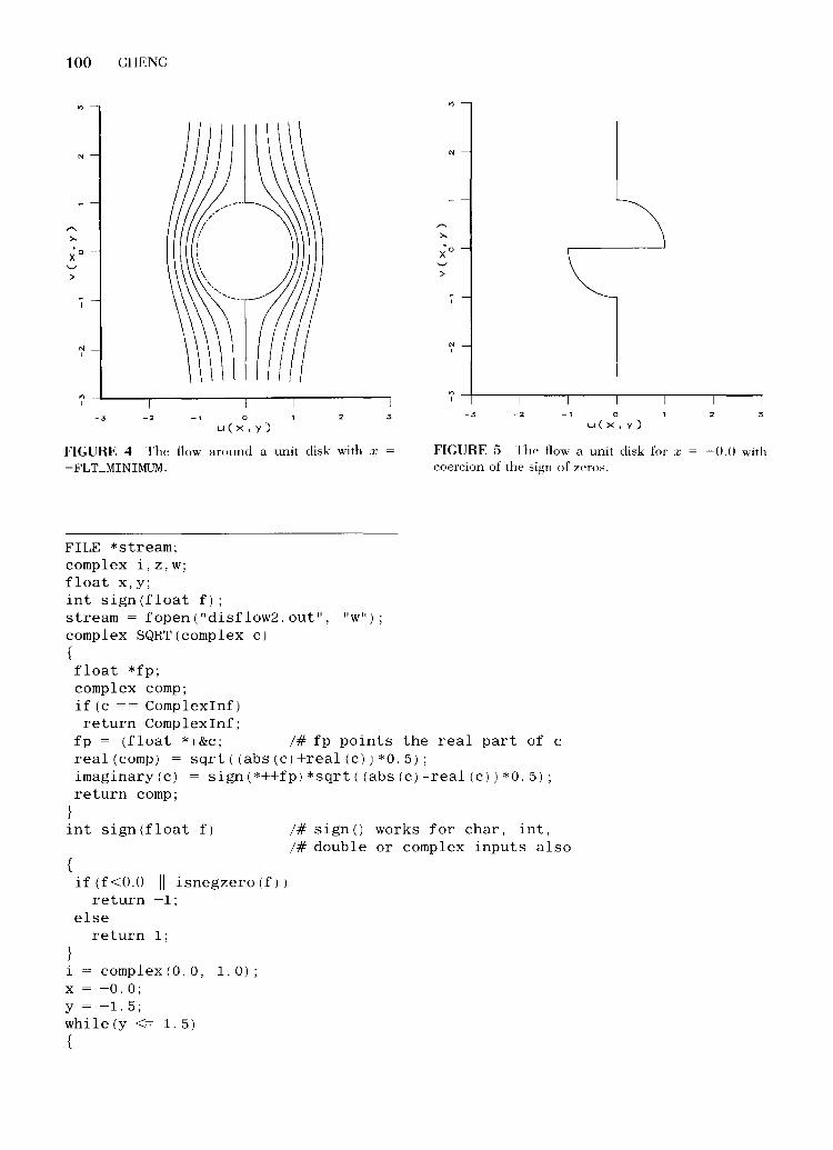
100 CHENG

-3 -2 2 _, 0

u(x,y) 3 -3 -2 _, 0

u(x,y)

FIGURE 4 The flow around a unit disk with x -FLT_MINIMUM.

FIGURE 5 The flow a unit disk for x coercion of the sign of zeros.

FILE *stream; complex i,z,w; float x,y; int sign(float f); stream = fopen ( "disflow2. out", "w") ; complex SQRT(complex c) { float *fp; complex camp; if (c == Complexlnf) return Complexlnf;

fp = (float *)&c; !# fp points the real part of c real(comp) = sqrt((abs(c)+real(c))*0.5); imaginary(c) = sign(*++fp)*sqrt((abs(c)-real(c))*0.5); return camp;

} int sign(float f)

{

}

if (f<O.O isnegzero (f)) return -1;

else return 1;

i complex(O.O, 1.0); X -0. 0; y -1. 5; while (y <= 1. 5) {

!#sign() works for char, int, !# double or complex inputs also

2 3

-0.0 with

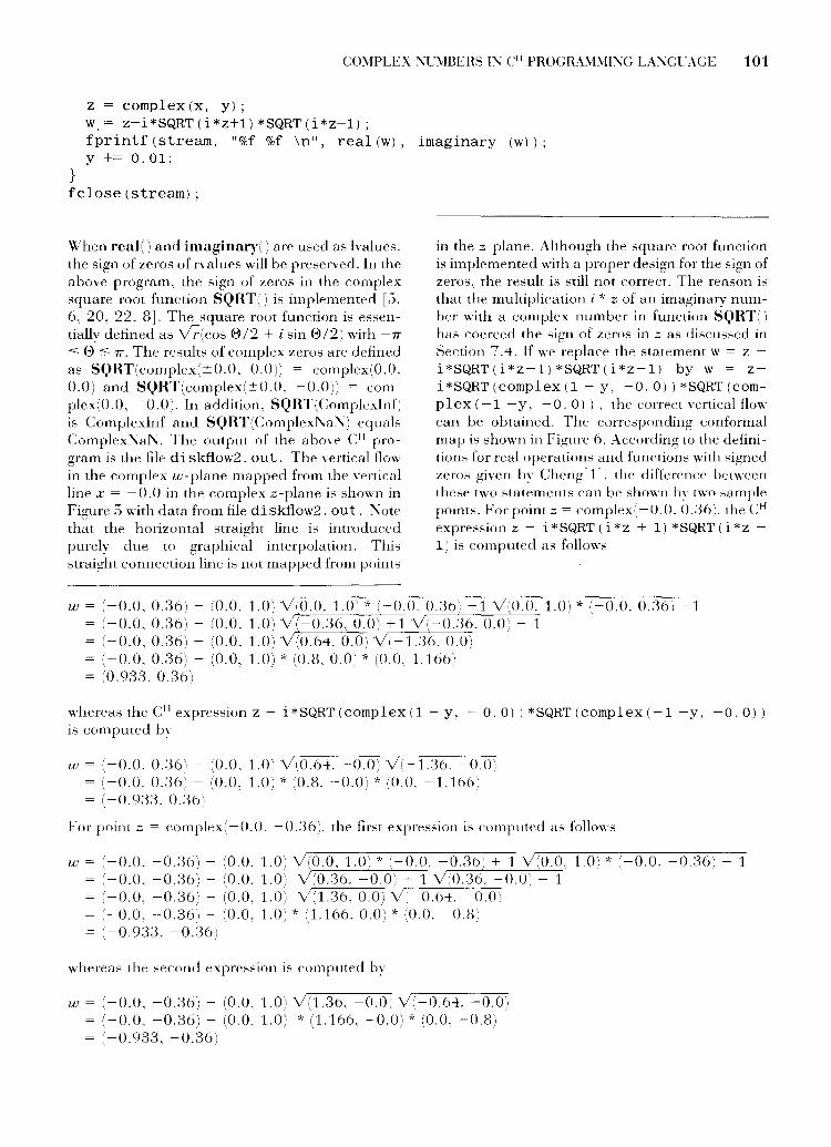
C0.\1PLEX .'\T.'.\IBERS I:\" C11 PROGRA.\1.\li:\"G LA:\GLAGE 101

z = complex(x, y); w.= z-i*SQRT(i*z+1)*SQRT(i*z-1); fprintf (stream, "%f %f \n", real (w) , imaginary (w)) ; y += 0.01;

} fclose (stream) ;

When real() and imaginary() are used as !values. the sign of zeros of rvalues will be preserved. In the above program. the sign of zeros in the complex square root function SQRT() is implemented [S. 6, 20, 22, 8]. The square root function is essen­tially defined as \./7(cos E>/2 + i sin E>/2) with -7r

:::; E> :::; 1r. The results of complex zeros are defined as SQRT(complex(±O.O. 0.0)) = complex(O.O. 0.0) and SQRT(complex(±O.O, -0.0)) = com­plex(O.O, -0.0). In addition, SQRT(Complexlnf) is Complexlnf and SQRT(Complex~a~) equals Complex]\;a~. The output of the above C11 pro­gram is the file di skfiow2. out. The vertical flow in the complex w-plane mapped from the vertical line x = -0.0 in the complex z-plane is shown in Figure 5 with data from file di skfiow2. out. 1'\ote that the horizontal straight line is introduced purely due to graphical interpolation. This straight connection line is not mapped from points

in the z-plane. Although the square root function is implemented with a proper design for the sign of zeros. the result is still not correct. The reason is that the multiplication i * z of an imaginary num­ber with a complex number in function SQRT() has coerced the sign of zeros in z as discussed in Section 7. 4. If we replace the statement w = z -i*SQRT(i*z+1) *SQRT(i*z-1) by w = z­i*SQRT (complex (1- y, -0. 0)) *SQRT (com­plex ( -1 -y, -0. 0) ) , the correct vertical flow can be obtained. The corresponding conformal map is shown in Figure 6. According to the defini­tions for real operations and functions with signed zeros given by Cheng[ 1]. the difference between these two statements can be shown by two sample points. For point z = complex(-0.0. 0.36). the CH expression z- i*SQRT (i*z + 1) *SQRT (i*z-1) is computed as follows

w = (-0.0. 0.36)- (0.0. 1.0) Y(O.O. 1.()': * (-0.0. ().;36) +1 V(O.O. 1.0) * (-0.0. 0.36) -1 ( -o.o. 0.36) - (o.o. 1.0) V ( -0.~36. o.o) + 1 Y( -o.:36. o.o; - 1 (-o.o, 0.36)- (O.o. 1.0) Y(0.64. 0.01 V(-1.:36. tLO)

= (-0.0. 0 .. 36)- (0.0. 1.0) * (0.8. 0.0) * (0.0. 1.166) = (0.933. 0.:36)

whereas the CH expression z- i*SQRT (complex (1- y, - 0. 0)) *SQRT (complex (-1 -y, -0. 0)) is computed by

w = (-o.o. 0.36)- (O.o. 1.0) Y(0.6-L -0.0) V(-1.:36. -0.0) = (-0.0. 0 .. 36)- (0.0. 1.0) * (0.8. -0.0) * (0.0. -1.166) = (-0.9:3:3. 0.36)

For point z = complex(-0.0. -0.36). the first expres,ion i:-; computed as follow,;

w = (-0.0. -0.:36)- (0.0. 1.0) Y(O.O. 1.0) * (-0.0. -0.:36) + 1 Y(O.O. 1.0) * (-0.0. -0.:36)- 1 (-o.o, -0.36) - (o.o. 1.0) V(o.:36. -o.o: + 1 V(0.36. -o.o) - 1 (-o.o, -0.36)- (0.0. 1.0) Y(1.36. o.o) Y(-0.64. -o.o; (-0.0. -0.36)- (0.0. 1.0) * (1.166. 0.0) * (0.0. -0.8) (-0.9:)3. -0.36)

whereas the second expression is computed by

w = (-o.o. -0.36)- (O.o. 1.0) Y(1.36, -o.o) V(-0.64. -o.o) = (-0.0. -0.36)- (0.0. 1.0) * (1.166. -0.0) * (0.0, -0.8) = (-0.933, -0.36)

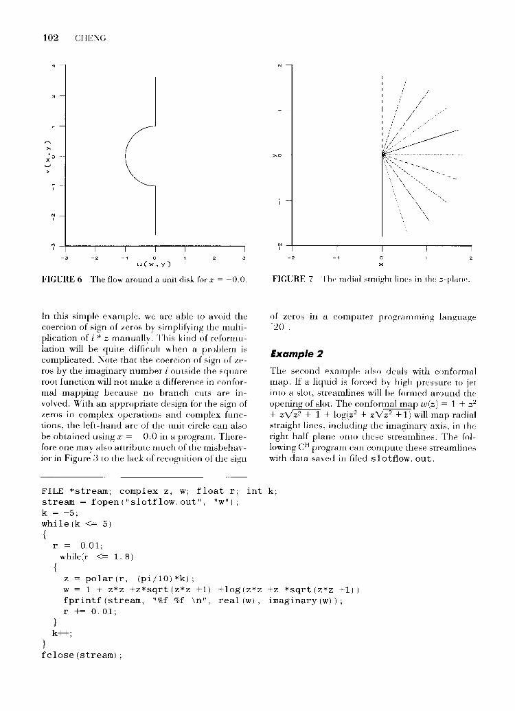
102 CHE'\iG

-3 -2 _, 0 2 3

u(x,y)

FIGURE 6 The flow around a unit disk for :x: = -0.0.

In this simple example, we are able to avoid the coercion of sign of zeros by simplifying the multi­plication of i * z manually. This kind of reformu­lation will be quite difficult when a problem is complicated. l\"ote that the coercion of sign of ze­ros by the imaginary number i outside the square root function will not make a difference in confor­mal mapping because no branch cuts are in­volved. With an appropriate design for the sign of zeros in complex operations and complex func­tions, the left-hand arc of the unit circle can also be obtained using x = -0.0 in a program. There­fore one may also attribute much of the misbehav­ior in Figure 3 to the lack of recognition of the sign

-2 _,

I

/ /

I ' I I / /

:l<~· .... ';.··

\\'"':. ... - ..... -·.\><~" ............ ..

\ ' \

\

/

/ /

/

\ ',

0

X

\

\ \

\

2

FIGURE 7 The radial straight line~ in the z-plane.

of zeros m a computer programming language [20].

Example2

The second example also deals with conformal map. If a liquid is forced by high pressure to jet into a slot. streamlines will be formed around the opening of slot. The conformal map w(z) = 1 + z 2

+ zV z2 + 1 + log(z2 + zY z 2 + 1) will map radial straight lines. including the imaginary axis, in the right half-plane onto these streamlines. The fol­lowing CH program can compute these streamlines with data saved in filed slotfiow. out.

FILE *stream; complex z, w; float r; stream = fopen ( 11 slotflow. out 11

, 11 W 11

) ;

k = -5;

int k;

while (k <= 5)

{

}

r = 0.01; while(r <= 1. 8)

{ z = polar (r, (pi/10) *k); w = 1 + z*z +z*sqrt(z*z +1) +log(z*z +z *sqrt(z*z +1)) fprintf (stream, "%f %f \n", real (w), imaginary (w)); r += 0. 01;

} k++;

fclose (stream) ;

CmJPU:X :\"C\IBEHS 1:\" <:1 1 PHOGH\.\L\IL\G L\:\"CL\CE 103

'

~-;::;;}:~< //

~~<~:--<,,-I. I i I i

l

0 -+------------,------------,----------~ I

-5 0 5 10

u(x,y)

FIGURE 8 The flow forced into a slot in the u•-plane with z = polarlr. (})or z = complex!FLT_\11:\"IMl .\I. Y).

The radial straight lines in the z-plane and corre­sponding images in the w-plane are shown in Fig­ures : and 8. respectively. Points along radial straight lines in the z-plane are generated by the function polar(r.theta). where r runs from 0.01 to 1.8 with a step size of 0.01 and theta from -1r12 to 1rl2 with a step size of 1r110. If r in the above program is 0. w will be Complexlnf: correspond­ingly. real(w) and imaginary(w) become :\"a~s. It appears in Figure 8 that complex infinities in the w-plane are located in (u. u) = -x + (y with -7r 12 :::; y 1rl2 for different streamlines: but. there is actually only one complex infinity. The origin of the z-complex plane is mapped to Complexlnf in the extended finite complex plane in a one-to-one manner with w(complex(O.O, 0.0)) = Complexlnf. In CH, all points on the w-plane with their real parts less than -FLT_MAX are treated as Com­plexlnf as shown in Figure 2. The picture of w(zJ is symmetrical about the real axis because w(z) =

w(z). The conformal map can be viewed as fol­lows. Along the imaginary axis with x = 0. as ,Y

running from -x through -1 toward 0. and then from 0 through 1 toward x, the image in the w-plane runs from left to right along the lower wall and back along the lower free boundary of the jet toward infinity, then from the infinity to the upper free boundary, finally, from left to right along the upper free boundary and back along the upper wall. Interestingly, lower and upper free bound­aries and other streamlines can be considered to

merge at the infinity of Complexlnf in the w­plane. which corresponds to the origin of com­plex(O.O. 0.0) in the z-plane.

Note that there are slits in the imaginary axis with z 2 < -1 beyond ± i. Points generated by z =

polar (r, pi I 2) may not be exactly on the imaginary axis due to roundoff errors. lf we are cautious. we mav want to exarnine the behavior of this conformal map without the effect of roundoff errors introduced by the polar() function. To sup­press the contribution of the perturbation effect of roundoff errors. points along the imaginary axis in the z-plane can be generated by z = com­plex (0. 0, y). \\hen the two radial lines along the imaginary axis are calculated by z = com­plex(O.O, y) withy running from 0.01 to 1.8 and from -0.01 to -1.8. the corresponding images in the w- plane are plotted in Figure 9. Like the pre­vious example. the lower walL part of the image. disappears. which can be explained as follows. The walls u = i1r and u = -i1T' in the w-plane are the images of points in the imaginary axis z = (Y with .Y > 1 andy < -1, respectively. The curve forward from u = i1r then back to w = -lnf + i1r I 2 is the image of the segment of z = Zr with 0 < y < 1. ·when z = - iJ· withy> \,; w(z) becomes 1 - y 2

+ .YY.y2 - 1 + log(y2 - y .Y2 - 1) + i1r. which

will map the slit on the lower part of the imaginary axis onto the tiny segment of the upper wall as is shown in Figure 10. This result holds even if the

.............. I i i i

0 -+------------,------------,----------~ I

-5 0 5 10

u(x,y)

FIGURE 9 The flow forced into a slot in the w-plane ·with z = cornplex(O.O. y) for the imai!inary axis in the z­plane.

104 CHE:'\G

0 -+------------~----------~----------~ I

-5 0 5 10

u(x,y)

FIGURE 10 The true image in the w-plane for the negative imaginary axis in the z-plane.

sign of zeros is respected with -7r ::::: 0 ::::: 7T as proposed [20]. This phenomenon is due to the singularity along the slit. 1\ote that like the hori­zontal line in Figure S, the vertical straight line. which connects the tiny segment in u = i7T and the streamline in the lower part of Figure 10 .. is pro­duced by graphical interpolation. This straight connection line is not mapped from points in the z-plane. 1\evertheless, a small perturbation of x, when y runs from -oo to -1, can bring back the missing lower wall. How tiny should x be is a non­trivial question in most computer languages as pointed out by Kahan [20]. In C11 , however, there is a definitive answer to this question. If x for the imaginary axis in the program is set to any small positive number that is larger than or equal to FLT_MINIMUM, that is, z = complex (FLT_MINIMUM, y), the missing lower wall in Fig­ure 9 can be recovered. It is interesting to point out that if the conformal mapp~function is chosen as w(z) = 1 + z 2 + zVz + i ~ + log(z2 + zv;-+i ~), the tiny segment of the wall that appears in Figure 10 will become a full wall, but other behaviors like locations of slits remain the same.

The above two examples demonstrate that con­formal maps may misbehave along slits. However, a small perturbation normally will bring back the missing information. Decreasing the step size in a loop of a program may also recover the critical information, which resembles the handling of nu-

merical solutions for stiff differential equations in some aspects.

8 CONCLUSIONS

Complex numbers are generalization of real num­bers. Complex numbers are manipulated in the same manner as real nurnbers in CH. Because complex is implemented as a basic data type in the C 11 programming language, the numerical computation can be handled in a much integrated fashion. CH treats floating-point real numbers with signed zeros and complex numbers with un­signed zeros as well as 1\ot-a-l\umber and infini­ties in an integrated consistent manner.

For scientific computing with complex num­bers, the extended finite complex plane along ·with complex metanumbers of ComplexZero. Com­plexlnf. and Complexl\al\ are introduced in this article. The l/0 for complex numbers and data conversion rules between real numbers and com­plex numbers are defined. The results of complex arithmetic and relational operations. and poly­morphic mathematical functions with complex metanumbers as input arguments are also de­fined. These may be different from the results ob­tained directly according to their definitions for regular complex numbers. Besides the polymor­phic nature in which the algorithms and resultant data types of arithmetic operations depend on the data types of operands .. the algorithms and resul­tant data types of mathematical functions are re­lated to the input arguments: mathematical func­tion in CH can have a variable number of arguments. In case a function becomes a complex function, additional integral arguments in com­paring with its real counterpart indicate which branch of a multiple-valued complex function shall be invoked. It is the first time, I believe. that such simplicity is introduced in a general-purpose computer programming language for scientific computing with complex numbers. Example pro­grams show that the external complex functions in CH can be programmed in the same syntax of the ANSI C and treated as if thev were the internallv . . built-in functions.

The rationales for the decision of the designed features, related to complex numbers in CH. have been provided from language design, implemen­tation, and application points of views. We have demonstrated in CH programs the effective han­dling of branch cuts of multiple-valued complex functions that are difficult to handle for most other computer programming languages.

CO~IPLEX '\l ~IBEHS 1'\ C 11 PHOCHA~l~ll'\G L\'\CL\GE 105

ACKNOWLEDGMENTS

The author would like to thank the referees for their thoughtful comments that improved the quality of this article.

REFERENCES

[ 1] H. I I. Chenf!. ··Scientific Computing in the C11

Programming Languaf!e. Department of .\lechan­ical. Aeronautical and .\laterials Engineering.·· Cniversity of California. Davis. Technical Report TH-.\lA~lE-9:3-101. Fehruarv 18. 199:3.

[2] A'\SI. .cLYS/ Standard .\3. 9-197'1. Programming Language Fortran •.revision of A:\Sl X2.9-1966j. :\ew York: A'\SI. 19"78.

'31 C. S. Hodgson. ··Proposed Standard for Packaf!eS of Heal and Complex Type Declarations and Ba­sic Operations for Ada (including \ector and ~la­trix Types;.·· ACll Ada Lett .. vol. XI. 1991. pp. 91-130.

[ 4] G. S. Hodf!son. ··Rationale for Proposed Stan­dard for Packages of Real and Complex Type Declarations and Basic Operations for Ada (in­cluding \ector and .\latrix Typesj ... ACJJ Ada Lett .. vol. XI. 1991. pp. V31-1:39.

[.S] J. S. Squire. '·Proposed Standard for a Generic Package of Complex Elementar-v Functions.·· ACJJ Ada Lett .. vol. XI. 1991. pp. 140-16;-).

l6 J. S. Squire. ··Rationale for the Proposed Stan­dard for a Generic Package of Complex Elemen­tar-y Functions.·· ACJJ Ada Lett .. vol. XI. 1991. pp. 166-1:9.

[":'] D . .\1. Ritchie. and K. L. Thompson. ··The unix time-sharing system.·· Commun. ACU. vol. 1:. pp. 365-:3:5. 197 '±.

!8] B. \\. Kernighan and D . .\l. Ritchie. The C Pro­gramming Language. Englewood Cliffs. '\J: Prentice-Hall. Inc .. 1st edition (K be RC). 197 8: 2nd edition (A'\Sl C). 1988.

:9J B. Stroustrup. The c++ Programming Language. Reading . .\lA: Addison-,,.eslev. 198"7.

[10] IEEE. ot\SI/!EEE Standard 75-1-1985. f£1:"E Standard for BinaT)· Floating-Point Arithmetic, Piscataway. '\J: IEEE. 1985.

[11] A'\SL A.\SI Standard X3.1.59-1959. Program­ming Language C. :\ew York. A'\SI. 1989.

[12] R. \.Churchill. and J. \\.Brown. Complex Vari­ables and Applications 4th edition). '\ew York: .\1cGraw-Ilill. 1984.

[13] J. E . .\1arsden. Basic Complex Ana(l·sis. San Francisco. CA: \\. H. Freeman. 19"73.

[14] G. L., Steele. Jr., Common Lisp: the Language (2nd edition). Bedford . .\lA: Digital Press. 1990.

[15] S. Wolfram, Mathematica: A System for Doing Mathematics by Computer. Redwood City, CA: Addison-Wesley, 1988.

16, .\lath \\ orks. Pro-JJA TLAB Cser 's Guide. South '\tHick . .\lA: The .\lath Works. Inc .. 1990.

:1:1 A'\SI. ASSl/!EL'L' Stcmdard 770 X.J.97-19'1.'3.

[18]

r19 l .

[201

/L'EJ-: Standard Pasral Programming Language. Piscataway. '\.I: IEEE. 19~t3. C. Lanczos. ·'A precision approximation of the gamma function ... J. SJA:'vl .Yumerical Arza(n;is. Ser. B. vol. L pp. 86-96. 1964. \\·. II.. Press. B. P. Flannery. S. A. Teukolsky. and \\·. T. \·etterling . . \umerical Recipes in C: The Art of Scientific Computing. Cambridge . .\fA: Cambridge Lniversity Press. 1990. \\·. Kahan. ""Branch cuts for complex Plementan· functions or much ado about nothing· s sign bit.·· The State of the Art in .\umerical Ano(1·sis. Ox­ford: Oxford Lniversity Press. pp. Eio-211. 198"7.

·21· J. Thomas. Floating-point C extensions . . \'CEG X.'JJ11.1/98-00 . .Tan. 20.199:3.

[22] F. Tydeman. ··.\Ierging complex and IEEE-"745 ... Document X:3J11.1 ('\CEC: 92-061.

[23] H. H. Cheng. "Computations of dual numbers in the extended finite dual plane ... Proceedings of the 1998 AS.UE Design Automation Conference. Albuquerque and :\ew York: AS.\IE. 199:3. pp. :.3-80.

[24] P. Penfield. Jr.. ··Principal values and branch cuts in complex APL · · APL Quote Quad. vol. 12. pp. 248-256. 1981.

[25] H. Koher. Dictionary of Conformal Representa­tions. ~ew York: Dover Publications. Inc .. 19;S":'.

[26] H. Baker. ··Less complex elementary functions.·· AC.H SJGPLA.\ .\'otices. mi. 2"7 .. pp. 15-16. 1992.

[2"7] D. S. Collens .. ··Algorithm 243: logarithm of a complex number.·· Collected Algorithms From C40/ (vol. II). 1980.

~281 P. Friedland. "Algorithm 312: absolute value and square root of a complex number.·· Collected Algorithms From C.ICJ1. (vol. II). 1980.

[29] J. R. Herndon. ""Algorithm '±6: exponential of a complex number.·· Collected Algorithms From CACH (vol. I) 1980.

[30] J. R. Herndon. ""Algorithm '±8: logarithm of a complex numher. · · Collected Algorithms From CAC.l.J (vol. l). 1980.

[31 j J. R. Herndon ... Algorithm 53: nth roots of a com­plex number. .. Collected Algorithms From CAC.H (vol. l). 1980.

[32] .\1. L. Johnson and\\. Sangren. ··Algorithm 106: complex number to a real power. .. Collected Al­gorithms From CAC.U (mi. 1). 1980.

[33] H. Kuki, ·'Algorithm 421: complex gamma func­tion with error control.·' Collected Algorithms From CACM (vol. 1), 1980.

[3'±] C. \\. Lucas Jr. and C. \\". Terrill. ""Algorithm 404: complex gamma function ... Collected Algo­rithms From CACA! (vol. 1). 1980.

106 CHENG

[35] A. P. Relph, "Algorithm 190: complex power." Collected Algorithms From CAC:l1 (vol. I), 1980.

[36] R. L. Smith, "Algorithm 116: complex dh;sion. '' Collected Algorithms From CACM (vol. I), 1980.

[37] R. P. Van de Riet, "Algorithm 186: complex arithmetic." Collected Algorithms From CACM (vol. I), 1980.

[38] Dritz, K. W., "Proposed Standard for a Generic Package of Elementary Functions for Ada.'· Ada Numerics Standardization and Testing, ACM Ada Letters, vol. XI, No.7, Fall, 1991, pp. 9-46.

[39] W. Kahan and J. W. Thomas, "Augmenting a programming language with complex arith­metic," Document X3J11.1 (NCEG), pp. 91-039.

Submit your manuscripts athttp://www.hindawi.com

Computer Games Technology

International Journal of

Hindawi Publishing Corporationhttp://www.hindawi.com Volume 2014

Hindawi Publishing Corporationhttp://www.hindawi.com Volume 2014

Distributed Sensor Networks

International Journal of

Advances in

FuzzySystems

Hindawi Publishing Corporationhttp://www.hindawi.com

Volume 2014

International Journal of

ReconfigurableComputing

Hindawi Publishing Corporation http://www.hindawi.com Volume 2014

Hindawi Publishing Corporationhttp://www.hindawi.com Volume 2014

Applied Computational Intelligence and Soft Computing

 Advances in 

Artificial Intelligence

Hindawi Publishing Corporationhttp://www.hindawi.com Volume 2014

Advances inSoftware EngineeringHindawi Publishing Corporationhttp://www.hindawi.com Volume 2014

Hindawi Publishing Corporationhttp://www.hindawi.com Volume 2014

Electrical and Computer Engineering

Journal of

Journal of

Computer Networks and Communications

Hindawi Publishing Corporationhttp://www.hindawi.com Volume 2014

Hindawi Publishing Corporation

http://www.hindawi.com Volume 2014

Advances in

Multimedia

International Journal of

Biomedical Imaging

Hindawi Publishing Corporationhttp://www.hindawi.com Volume 2014

ArtificialNeural Systems

Advances in

Hindawi Publishing Corporationhttp://www.hindawi.com Volume 2014

RoboticsJournal of

Hindawi Publishing Corporationhttp://www.hindawi.com Volume 2014

Hindawi Publishing Corporationhttp://www.hindawi.com Volume 2014

Computational Intelligence and Neuroscience

Industrial EngineeringJournal of

Hindawi Publishing Corporationhttp://www.hindawi.com Volume 2014

Modelling & Simulation in EngineeringHindawi Publishing Corporation http://www.hindawi.com Volume 2014

The Scientific World JournalHindawi Publishing Corporation http://www.hindawi.com Volume 2014

Hindawi Publishing Corporationhttp://www.hindawi.com Volume 2014

Human-ComputerInteraction

Advances in

Computer EngineeringAdvances in

Hindawi Publishing Corporationhttp://www.hindawi.com Volume 2014