gy301 geomorphology lab 5: total station project … geomorphology lab 5: total station project data...

GY301 GeomorphologyLab 5: Total Station Project Data Collection

Introduction

For this lab you will use the Total Station to survey a topographic map of the campus areacorresponding to the area outlined in Figure 5. Your project can begin by choosing anyconvenient location in Figure 5 (ST01-ST20), however, make sure that you can resection to 3mirror targets established on benchmarks when setting up your instrument. If you can’t resectionto 3 target benchmarks backsight by coordinate to a benchmark after setting up the instrument onanother benchmark. Shoot back to that benchmark or another visible benchmark to verifyaccuracy. The mapping will use the UTM NAD27 zone 16 coordinate system, therefore, youmust make sure that your total station instrument is set to use meters. You can download a list ofthe benchmark UTM coordinates and elevations at:

http://www.usouthal.edu/geography/allison/GY301/TotalStationLabBenchmarks.xls

Total Station Setup

Your instructor will demonstrate for your group the leveling and initial setup of the Total Station.After leveling the instrument on a known benchmark location select another known point for thetarget (or use another Total Station instrument) for “locking-in” to the coordinate system (UTMNAD27). You will need a print-out of the UTM coordinates and elevations of the benchmarks,and you need to record the instrument height of the instrument in meters with a tape measure.Measure the height from the ground to the gray horizontal index line on the side of theinstrument. (NOTE: there are 3.28 feet per meter if you need to convert from feet to meters).

In general the Total Station step-by-step procedure for measuring UTM coordinate data goes asfollows:

1. Level the instrument2. Power up and initialize the instrument3. Select and make active the proper job name (i.e. “G1" for Group 1, etc.)4. Enter any XYZ data given to you (benchmarks, etc.) as “known data”.5. In the “[MEAS]” menu select “[COORD]” to define the station position, select a backsight,and test the calibration of the instrument. After this step you will be ready to collect data. Tosuccessfully complete this step you MUST have the instrument leveled on a known coordinatepoint, and the target must be setup on another known point.6. Continue to use [COORD] to collect data at target points in the mapping area:

a. Use “T01", “T02" for Group 1 tree control pointsb. Use “C01", “C02", etc. for Group1 corner points on buildings

Page -1-


c. Use “E01", “E02", etc. for ground surface topographic control pointsd. Use “I01", “I02", etc. for instrument station control points.

7. When you are shooting tree positions it will of course be impossible to place a target mirror inthe center of the tree therefore the “[OFFSET]” command should be used. The offset commandallows you to place the mirror target on the left or right of the target, or in front or behind thetarget. You can use a tape measure to measure the offset distance (must be meters for UTM)between the mirror target and the actual target position. See a detailed description below. Keep a notebook as backup on the X,Y,Z coordinates and notes on what each point collectedactually corresponds to (ex. C1 = NE corner of Student Union).8. Download the instrument data to an Excel spreadsheet for contouring and posting with QGIS.

All of the survey gear except for the Total Station and batteries will be stored in the trailer. Makesure you return this gear to the trailer and lock the trailer when finished. Return the Total Stationto your instructor.

A detailed description of operating the SET610 Total Station for the above steps follows below.The description uses references to the SET610 user manual so make sure it is accessible.

Step 1: Level the instrument

Refer to the SET 610 manual section 7.

Comments:

When first placing the tripod over the benchmark make sure that the legs are extended toapproximately chest height of the shortest person that will be using the instrument. Make sure thetripod head is approximately level, and then look directly down through the centering screw toensure that the tripod is centered or nearly centered over the benchmark aluminum plate. If it isnot, pick up the tripod and move it so that it is centered. Proceed to mount the instrument on thetripod.

A common mistake is to skip the step at the end where you shift the instrument to center theoptical plummet on the benchmark. (Section 7.2, step 7). If someone accidentally “bumps” thetripod after the instrument is leveled causing the “out of range” error (un-leveled), simply repeatsection 7.2.

Step 2: Power-up and Initializing the Instrument

Page -2-


Refer to sections 6.1 and 6.2 for charging and installing the SET 610 battery. Press the “on”button to power-up the instrument. The instrument always initially activates to the [MEAS](measurement) menu. Press the “ESC” button to backup to the main (top) menu.

Initializing the instrument allows one to enter useful data and settings in the comfort of the officeto reduce time on-site. For this project you need to first clear out any data left from previousprojects, and set units and job name. Also, benchmark data may be entered as known data at thistime to reduce the amount of typing on-site.

From the top menu select [CNFG] (configuration), and then “Obs. condition”. Cursor to the“Coord.” option. Use the right or left cursor to change the coordinate format to “E-N-Z” (easting 1st, northing 2nd, elevation 3 ). Press <enter> key to select the “E-N-Z” format. Press <ESC> tord

return to the Config menu.

Cursor up or down in the “Config” menu until “Unit” is selected and press <enter>. Cursorup/down until “Dist” is highlighted, and then use the right/left cursor until “meter” is highlighted,and the press <enter>. Press <ESC> to return to top menu.

Step 3: Select a Job Name

From the <MEM> menu select “Edit Job Name” and set the name to match your group. Change“JOB1" to “G1" for group 1 for example. Make sure that the new job name is selected as theactive job.

Refer to section 22.1 in the manual.

NOTE: If you don’t select a job name the name will default to “JOB1".

Step 4: Enter Known DataSince all of the benchmarks have been previously surveyed in UTM NAD1927 coordinates itmakes sense to enter all of the benchmark data into the instrument before actually setting it upon-site to collect data. This speeds up the setup of the instrument because you can occupy anybenchmark and use any other benchmark as the backsight for calibration. Rather than having totype in the long UTM coordinates on-site you can do this in the office. Even if you do this on siteit is convenient to do this since you will never have to re-type the coordinates if you have to usethe benchmarks in a future setup. Also, all of the benchmark data can be used to generatecontours in Surfer so you should add all of the points eventually anyway.

Refer to section 23.1 to enter known data. You will need the spreadsheet printout of benchmark

Page -3-


data at this point.

If the known data has been pre-loaded into the instruments your instructor will let you know.Regardless, you should double check the coordinates against the online spreadsheet values.

Step 5: Backsight or Resection Instrument

Backsighting the total station instrument “locks” the instrument into a designated mappingcoordinate system. For this project this will be UTM NAD27 coordinates. There are 2 differentways to backsight: by angle and by coordinate. We will use the “by coordinate” method becausewe already have a pre-defined network of benchmarks on campus surveyed in UTM coordinates.Before backsighting the instrument should be leveled initialized on one of the benchmarks, andthe mirror target should be visible on another benchmark point. At this point you may want toreview section 8 on “Focusing and Target Sighting”. Also, measure the instrument height andverify the target height at this time. Use meters!

Refer to section 12 on “Coordinate Measurement” to backsight instrument.

Comments:

In this section setting the “horizontal azimuth angle” is conceptually the same as backsighting theinstrument.

Remember that wherever XYZ coordinates can be entered on a screen you can alternativelyselect the [READ] function key to read XYZ from a previously stored “known” data point (or apoint recorded through shooting a target). If all of the benchmark points have been previouslyentered as known data you can quickly backsight from any benchmark point.

After the station coordinates and the backsight coordinates have been specified make sure youselect the “Yes” option on the last screen to lock in the coordinate system. If you do not hit “Yes”the coordinate system used by the instrument remains random, and that means any data collectedis incorrect.

Remember that the backsight procedure is simply an alignment of the instrument to an azimuthindicated by the XYZ coordinates of the occupied and backsight points. It is very important thatthe vertical cross hair be aligned exactly on the target before indicating “yes” on the coordinatebacksight.

To ensure that the backsight “lock-in” to the UTM system is correct, you need to “shoot” it as if

Page -4-


it were a regular data point and compare the XYZ values obtained with the ones listed in thespreadsheet. They should be with several cm’s of the listed values for X, Y and Z. Press <ESC>from the backsight menu until you see “Observation”. Site the target on the benchmark used forthe backsight and press <enter> with “Observation” highlighted. Compare the coordinates. Theyshould agree to within several cm’s for XYZ. (NOTE: you can use any known point to test theinstrument calibration- it’s just more convenient to use the backsight point since your target isalready there).

Step 6: Use the [COORD] function to Collect Data

Refer to section 12.3 in the manual for 3D coordinate measurement details.

Comments:

Use the [COORD] function from the [MEAS] menu to measure and record the position of pointswhere the mirror target can be positioned directly on the target. This will be true of all of theelevation control points and the building corners.

Remember that if you have already backsighted for the session that you don’t have to redo thatprocedure unless you suspect the instrument has been accidentally moved.

You can change the target height or instrument height within this menu if needed. The targetheight may change often if you are shooting over shrubs or vehicles. Make sure these values areupdated before recording. If you record a point with an incorrect target height, re-shoot andrecord over the existing point.

NOTE: You can use the “resection” method to determine the XYZ coordinates of an instrumentposition if you can sight 3 or more benchmark positions. Refer to section 13 in the manual.

Step 7: Use the [OFFSET] function to Measure Obscured Points

Refer to section 18.1 Single-distance Offset Measurement.

Comments:

Use the offset command to shoot targets that you do not have a direct line-of-sight to, forexample a bush may obscure the corner of a building that needs to be surveyed. If you can’textend the target height to see over the bush the next best option is single-distance offset.Remember these requirements for single-distance offset:

Page -5-


1. You will need a 2 person with the target to use the tape measure to measure thend

offset.2. The mirror target will be set up either right, left, front or behind relative to the actualtarget. If it is right or left, a line drawn from the instrument to the actual target to themirror target should turn a 90 degree angle. In other words, the distance from theinstrument to the mirror target should equal the distance from the instrument to the actualtarget. If the mirror target is in front of, or behind the actual target it should be in exactalignment with the line extending from the instrument through the actual target. 3. Measure the offset distance with the same care and precision as you do the instrumentheight - 1 cm or less accuracy.

Select the [OFFSET] function from the [MEAS] menu. Then select “Offset by distance”.Position the mirror target either left, right or in front of the tree target and press the “[Obs]”function. The XYZ coordinates listed are the coordinates of the mirror target- not the tree. Editthe offset distance to match the distance measured with a tape from the center of the tree to themirror target. This should be in meters measured to 1 cm accuracy. Use the cursor key to changethe arrow indicator to point right, left, front to match the mirror target position. Selecting the[OK] function adjusts the observed XYZ to take into account the offset. The calculation assumesthat the angle inscribed by drawing a line from the instrument to the center of the tree target tothe mirror target is a 90 degree angle if right or left was chosen, in line with the instrument andtarget otherwise.

NOTE: For this lab you will need lots of data to generate an accurate topographic contour mapwith QGIS. There is no set minimum number but most groups collect about 1100 points over the3 weeks we spend on the project. Note that some points are outside the map boundary area- thatis OK because it helps control the contours as they exit the map area.

Step 8: Downloading the data from the SET 610

In order to download data from the SET 610 to a file you need the data cable and the “SokkiaProLink” software installed on a computer. Connect the cable to the SET610 and the serial portof the host computer. Start the ProLink software and power up the SET610. In the [MEM] menuselect “Job” and then the appropriate “JOB” name. Then proceed to “Comm setup” settings. Setthe following communications port parameters:

Baud rate: 9600 baudData bits: 8 bitsParity: noneStop bit: 1

Page -6-


Xon/Xoff: noChecksum: no

Back out of the menu to “Comms output”. Cursor up/down to your job name. Note that any“Known Data” that was entered into the instrument will also be downloaded no matter which jobname is selected. Hit the <enter> key to select job name. The number of data points in the joblisted to the right of the job name should now change to “out”. Select the <F4> key to “OK” thedownloading of the job. Cursor up/down to select “SDR” on the next screen, but do not hit theenter key yet (you will do that later).

1. Start the “ProLink” application from the start menu. Find the “Download/Upload” button onthe toolbar and select it. The Download/Upload window should now display. At the bottom ofthe screen set the device type to “SDR33/31 (SDR) format”.

2. Select the “Settings” button to check the communications port setup (Figure 1). Make surethat the port number matches the port that the cable is connected to on the computer (generallyCOM1), and that the communications parameters match those on the SET610 (generally 9600baud, 8 data bits, 1 stop bit, No parity). These settings must match those set on the Total Station“Comms setup”.

3. Select the “Connect” button option. The right window should display “Use Job Name SDR”.This means that the downloaded file will have the same name as the job name with an SDRextention. The “Connect” button should change to “Disconnect”. In the left window navigate tothe folder where you want the downloaded file to be sent. Now highlight the “Use Job NameSDR” in the right window (see Figure 2), then select the left pointing arrow between the 2windows. The ProLink program is now waiting to receive data from the SET610.

4. On the total station hit the <enter> button to send the data to the computer. You can now exitout of ProLink.

5. The downloaded SDR file is a simple text file that can be imported into Excel. Figure 3displays the SDR file in Notepad.

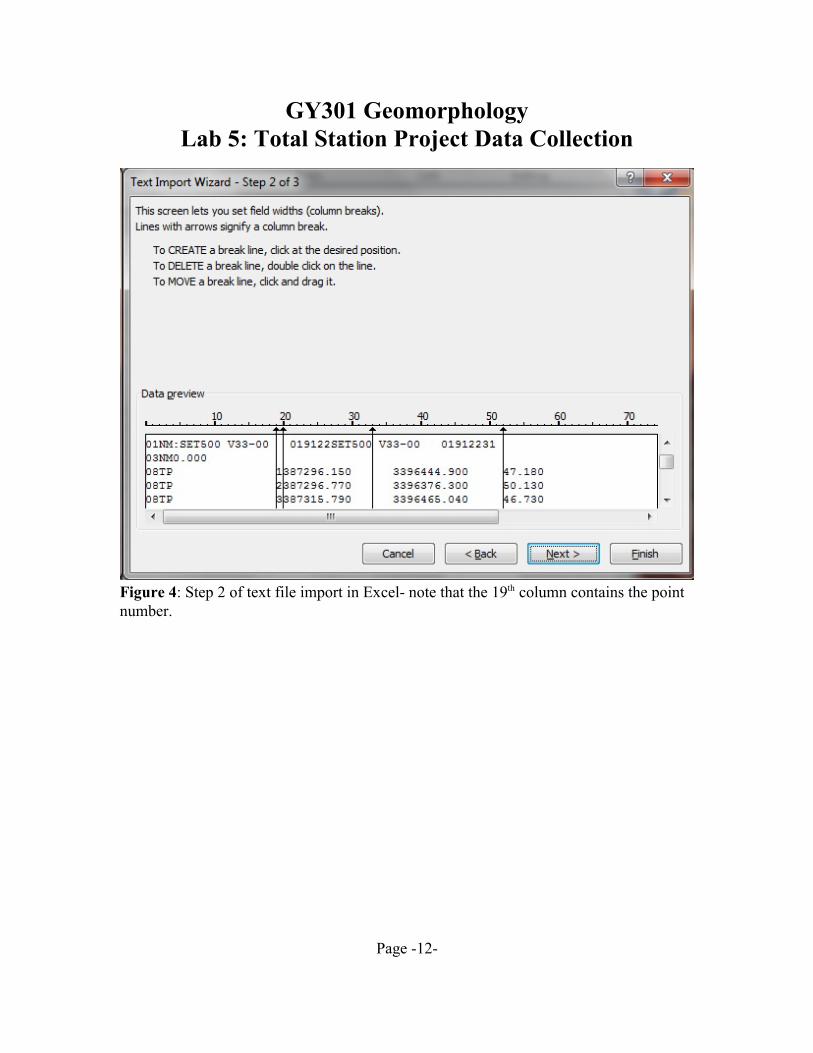
6. You will now need to import the file into Excel so that it can be used by QGIS. Start Excel andthen open the downloaded SDR file. Excel will automatically recognize that the file is a “text”file and pop-up an import menu. Select the “fixed column width” option and proceed. Set thecolumn widths so that the point number is separated from the easting (UTM X coordinate)number (Figure 4).

Page -7-


After importing the data copy just the easting, northing, and elevation data along with pointidentifiers to the 2 worksheet. Add headers so that when imported into QGIS you will seend

“UTM_X” or “Easting” when QGIS refers to the data column.

.

Page -8-


Figure 1: Port settings window in ProLink.

Page -9-


Figure 2: ProLink “download/upload” window.

Page -10-


Figure 3: Downloaded data file (.SDR) in Notepad.

Page -11-


Figure 4: Step 2 of text file import in Excel- note that the 19 column contains the pointth

number.

Page -12-


Figure 5: Campus aerial base map with location of survey benchmarks.

Page -13-

gy301 geomorphology lab 5: total station project … geomorphology lab 5: total station project data...

Documents