guidance for analysis of soil contamination using a ... · sampling locations for site...

Waikato Regional Council Technical Report 2016/22

Guidance for analysis of soil contamination using a portable x-ray fluorescence spectrometer www.waikatoregion.govt.nz ISSN 2230-4355 (Print) ISSN 2230-4363 (Online)

Prepared by: Pattle Delamore Partners Ltd For: Waikato Regional Council Private Bag 3038 Waikato Mail Centre HAMILTON 3240 September 2015 Document #: 4019546

Doc # 4019546

Peer reviewed by:

Date August 2016 Dr Nick Kim, Massey University Michelle Begbie, Waikato Regional Council

Approved for release by: Date September 2016 Dominique Noiton

Disclaimer

This technical report has been prepared for the use of Waikato Regional Council as a reference document and as such does not constitute Council’s policy. Council requests that if excerpts or inferences are drawn from this document for further use by individuals or organisations, due care should be taken to ensure that the appropriate context has been preserved, and is accurately reflected and referenced in any subsequent spoken or written communication. While Waikato Regional Council has exercised all reasonable skill and care in controlling the contents of this report, Council accepts no liability in contract, tort or otherwise, for any loss, damage, injury or expense (whether direct, indirect or consequential) arising out of the provision of this information or its use by you or any other party.

Doc # 4019546

Auckland Tauranga Wellington Christchurch

PATTLE DELAMORE PARTNERS LTD

Guidance for Analysis of Soil Contamination Using a Portable X‐Ray Fluorescence Spectrometer

Waikato Regional Council

solutions for your environment

A02719100R001_FINAL.DOCX

PATTLE DELAMORE PARTNERS LTD Level 4, PDP House 235 Broadway, Newmarket, Auckland 1023 PO Box 9528, Auckland 1149, New Zealand

Tel +64 9 523 6900 Fax +64 9 523 6901 Website http://www.pdp.co.nz Auckland Tauranga Wellington Christchurch

Guidance for Analysis of Soil Contamination Using a Portable X-Ray Fluorescence Spectrometer

• Prepared for

Waikato Regional Council

• September 2015

http://www.pdp.co.nz/

i i

G U I D A N C E F O R A N A L Y S I S O F S O I L C O N T A M I N A T I O N U S I N G A P O R T A B L E X - R A Y F L U O R E S C E N C E S P E C T R O M E T E R

A02719100R001_Final .docx P A T T L E D E L A M O R E P A R T N E R S L T D

Executive Summary

This document provides background information for, and describes procedures to be used, when undertaking field portable X-ray fluorescence (XRF) measurements of soils. Specifically, this guidance document provides:

• Best practice that should be followed for the sampling and analysis of soils which may have been impacted by metal and metalloid contamination.

• Guidance on the interpretation of data obtained from field XRF measurements of soils.

Field portable XRF analysis is an ideal tool to undertake a large number of measurements of elemental concentrations in the surface layers of soils in a very short time. However, the technique is subject to a number of sampling and analytical errors and is therefore regarded as a screening level or semi-quantitative assessment tool only. The main sources of error affecting accuracy of this technique are sampling error due to heterogeneity in the elemental distribution in the soil and moisture content variation in the sample. Therefore, properly preparing the soil sample is vital to assure good data quality. Another issue that may affect interpretation of results is that detection limits for some elements such as arsenic are not particularly low.

This document outlines the theory of X-ray fluorescence, the interferences and other factors which can influence the reliability of the XRF results, sample analysis procedures (including QA/QC measures) and minimum reporting requirements for undertaking XRF investigations.

In-situ XRF analysis (by placing the XRF directly in contact with the ground) requires minimal sample preparation but is only a screening level technique. BS/ISO standard 13196 (2013) provides a suitable methodology for undertaking the screening level investigations. Screening level analysis can be used for:

• Identifying potential hotspots on a site,

• Providing an indication of the extent of contamination,

• Preliminary identification of inorganic contaminants of concern present,

• Pre-selection of samples for analysis in laboratory,

• Selection of contaminants of concern for laboratory analysis,

• Identification of homogeneity/heterogeneity of soils,

• Assisting with remediation decision making,

• Site investigation prioritisation, and

• Screening of hazardous waste.

i i i



Semi-quantitative XRF analysis can be achieved by implementing more intensive ex-situ sample preparation, correct QA/QC techniques and careful use of the XRF to obtain best performance. Sieving, drying and homogenisation of soil samples removes many of the sampling errors caused by grain size effects, moisture content and other matrix effects, and increases the accuracy and reliability of the results. US EPA Method 6200 provides a methodology for undertaking semi-quantitative investigations.

Semi-quantitative investigations can:

• Assist with determining the appropriate soil sampling density and sampling locations for site investigation works (exploratory level site investigations);

• Provide an indication of degree of heterogeneity of elements present on the site;

• Provide additional data for assessing potential human health risk of average exposure to the site, provided that investigation objectives (outlined in Section 4.4) are met and suitable verification of results has been undertaken;

• Add to Preliminary Site investigation, assisting (along with traditional information sources) to determine if it is more likely than not that the site is contaminated.

Field portable XRFs can be misused or the data misinterpreted (in particular placing too much faith in the accuracy of the data) and therefore it is important that quality assurance/quality control procedures are in place when undertaking a semi-quantitative investigation for regulatory purposes; to minimise the errors in the application of results and demonstrate the data derived from the XRF investigation is fit for purpose. This includes undertaking an assessment of total uncertainty measurements (including sampling and analysis errors) to allow scientifically defensible decisions to made using the XRF data set.

i v



Table of Contents

S E C T I O N P A G E

Executive Summary ii

1.0 Introduction 1 1.1 Acknowledgements 1

2.0 The Place of Field Portable X-ray Fluorescence in Contaminated Site Investigations 2

2.1 Advantages and Disadvantages 2 2.2 Use of Field Portable XRF 4 2.3 FP-XRF Sampling Strategies 7

3.0 Elements Suitable for XRF Analysis 9 3.1 Factors which Influence Limits of Detection 9

4.0 Factors Affecting XRF Analysis Accuracy 11 4.1 Interferences and Sources of Error 11

5.0 XRF Safety Considerations 15

6.0 Sample Analysis Procedures 15 6.1 On-site Analysis 15 6.2 Quality Assurance/Quality Control 20

7.0 Data Analysis and Interpretation 24

8.0 Reporting on Results 25

9.0 References 26

Glossary – A Guide to Common X-Ray Fluorescence Terms 30

Table of Figures

Figure 1: Data Quality versus Information value (adapted from US EPA, 2001) 3

Table of Tables

Table 1: Advantages and Disadvantages of Field Portable XRF Spectrometers 2

Table 2: Variation in Limit of Detection for Different Soils and Measuring Times 10

v



Appendices

Appendix A: Theory of X-Ray Fluorescence

Appendix B: Analytical Lines and Spectral Overlaps

Appendix C: Detection Limits for FP-XRF for Selected Elements

Appendix D: Flow Charts Outlining the Processes of XRF Field Analyses of Soils

Appendix E: Calculating Uncertainty of Measurement

Appendix F: Data Comparability Checks

Appendix G: Summary XRF Report Checklist

1



1.0 Introduction

This document provides background for, and describes procedures to be used, when undertaking field portable X-ray fluorescence (FP-XRF) measurements of soils. Specifically, this guidance document provides:

• Best practice for the sampling and analysis of soils which may have been impacted by metal/metalloid contamination.

• Guidance on the interpretation of data obtained from field XRF measurements of soils.

This document is not intended to be an analytical training manual or to cover procedures for laboratory-based XRF instruments. Nor is this guidance intended to provide advice on the methods for undertaking screening of hazardous waste (such as e-waste or determining the presence of lead paint in building materials). If such investigations are to be undertaken, reference should be made to the appropriate standard method or international best practice guidelines, e.g. ASTM E1916-11, ASTM E2120 or IEC 62321 for hazardous waste screening and ASTM E2115-06 and E2271-05a for lead hazard assessments of dwellings.

Field Portable X-ray Fluorescence Spectrometry (FP-XRF) is a quick method for determining the total elemental composition of surface layers of in-situ soils or ex-situ soil samples. However, as FP-XRF is not capable of measuring the concentration of every element, other analytical techniques must be utilised for determining the concentration of some elements and organic compounds (such as hydrocarbons) if these are potential contaminants of concern.

While FP-XRF may provide an economical approach to site characterisation, it should not be regarded as always a cheaper method and, given it limitations, nor should it be regarded as a replacement for laboratory analysis. Rather, the best use of this technique is in combination with laboratory analysis, to provide a more complete picture of the extent of contamination present at a site and therefore increase certainty of decision making. Its speed of use, but lower accuracy, can provide a large number of semi-quantitative measurements that, when combined with confirmatory laboratory samples, can provide a better characterisation of contamination than a small number of more accurate laboratory analyses.

This guidance should be read in conjunction with the current version of the Ministry for the Environment’s Contaminated Land Management Guidelines No. 5: Site Investigation and Analysis of Soils.

1.1 Acknowledgements

This report is based on an earlier report prepared for the Marlborough District Council (PDP, 2013). The contribution of Marlborough District Council is

2



acknowledged. PDP would also like to thank Dr Nick Kim (Massey University) for peer reviewing this document.

2.0 The Place of Field Portable X-ray Fluorescence in Contaminated Site Investigations

2.1 Advantages and Disadvantages

Field portable X-ray fluorescence spectrometers are a useful tool for undertaking contaminated site investigations and guiding site remediation. They can provide rapid information in the field over a wide range of elements (usually, in order of atomic number, potassium (11) to uranium (92) for most instruments). This may be of practical benefit in identifying soils which need to be removed from a site, deciding which landfill particular soil should be consigned to, or undertaking adaptive sampling strategies. However, like all sampling and analysis techniques, FP-XRF has limitations. The main advantages and disadvantages of FP-XRF are outlined in Table 1 below.

Table 1: Advantages and Disadvantages of Field Portable XRF Spectrometers

Advantage Disadvantage

Simultaneous multi-elemental characterisation.

Need for laboratory check for semi-quantitative analysis, which can add to the project costs and delay.

Minimal sample preparation for in-situ analysis.

Detection limits higher than laboratory analysis (at best semi-quantitative). This requires careful consideration as to applicability for the particular project.

Allows on-site, real-time decisions (especially during remedial works or when using adaptive sampling techniques).

More reliable (accurate) for some elements than others due to potential interferences.

Allows prioritisation of sample analysis. Due to the small sample size, heterogeneity of the sample may result in high levels of measurement uncertainty.

May be cheaper per sample when large numbers of samples are being processed.

Can only measure certain elements.

Cannot measure any organic contaminants, e.g. organochlorine pesticides, petroleum hydrocarbons.

Cannot measure trace element speciation or determine oxidation states of metals.

3



Field portable XRF can be cheaper per sample than traditional laboratory analysis (especially if several analytes are being measured) and therefore a greater number of samples can be analysed for the same budget. However, the sample preparation required for best performance (semi-quantitative analysis) will reduce or may even eliminate this cost advantage, particularly as a proportion of samples must be submitted for confirmatory laboratory analysis.

Although FP-XRF is less precise and more likely to have a greater measurement bias than laboratory analysis, increasing the density of sampling with in situ measurements can be a relatively small incremental cost. This can result in the extent of contamination being better defined, with the benefit of lower likelihood of incorrectly classifying a site due to insufficient site characterisation.

This is illustrated in the diagram below, in which a few high quality data points (e.g. laboratory analyses) will provide a less “defensible” conclusion than many lower quality data points, and is based on the concepts of effective and defensible data developed by both the United States Environmental Protection Agency (US EPA, 2001) and the England and Wales Environment Agency (EA 2009).

Figure 1: Data Quality versus Information value (adapted from US EPA, 2001)

4



This means that for the FP-XRF, the fact that the technique will give higher bias and lower precision compared to laboratory analysis1 does not necessarily mean that the technique is invalid for human health or environmental risk assessment purposes, if:

• The precision of the data and potential bias are clearly quantified and incorporated into the sampling design and risk assessment;

• Laboratory results are used to validate the XRF results and support the conclusions made in the report.

This recognises that much of the uncertainty in environmental data does not come from the analysis method (whether using laboratory-based methods or field screening techniques) but from the sampling process itself inadequately representing the contaminant spatial variability.

Sections 6.2 and 7.0 provide further information regarding quality assurance/quality control protocols.

2.2 Use of Field Portable XRF

When used for in-situ soil measurement of elements, FP-XRF instruments are suitable for no more than qualitative or screening level assessment (ISO 13196:2013; Innov-X, 2003). This is not least because accurate analytical testing requires a uniform, homogeneous sample matrix, which will not normally be obtained with in-situ measurement.

Pre-measurement sample preparation, using limited sample pre-treatment (sieving and homogenising of the soil sample) is likely to produce better analytical data quality and may overcome some of the issues associated with heterogeneity. If the sample preparations described in Section 6.1.2.2 are followed then FP-XRF can provide semi-quantitative results.

If quantitative results are needed (equivalent to normal laboratory analysis), sample pre-treatment with drying, sieving, homogenisation and particle size reduction is necessary and analysis should be undertaken with laboratory equipment by an IANZ accredited laboratory. This is beyond the capability of FP-XRF and is therefore beyond the scope of this document.

As neither FP-XRF screening level nor semi-quantitative assessments meet the quality requirements normally expected for undertaking human health risk assessment or validation after concentration-reduction remedial work, FP-XRF should not be relied upon as the sole source of information for such purposes.

1 It should be noted that any analysis of environmental samples to determine contaminant concentrations (whether laboratory based or field based) is only ever an estimate of the true value of the concentration because all analytical methods are subject to uncertainties and bias.

5



The broad characteristics of screening and semi-quantitative investigations are described in the next sections.

2.2.1 Screening level investigations

A screening level investigation is a rapid, non-rigorous site investigation method which does not offer a definitive quantification of the concentration of the elements present. This type of investigation involves little or no sample preparation (therefore the results may be subject to high levels of uncertainty) and little quality assurance around the data. The results of this type of investigation by themselves cannot be used to verify compliance with threshold values or site remediation goals.

Typically, a screening level investigation can be used for such things as:

a. Providing preliminary identification of inorganic (e.g. heavy metal) contaminants and verifying the contaminants of concern tentatively identified in a conceptual site model;

b. Identifying locations with high contaminant concentrations on a site (such as location of sheep dip, CCA treatment bath, some chemical spills, orchard spray shed/spray mixing area2 or lead-based paint contamination around a house);

c. Providing an indication of the spatial extent and spatial variability of inorganic contamination;

d. Carrying out a preliminary screening for prioritising further investigation;

e. Screening sub-samples in a composite to identify if any sub-samples contain high concentrations of an element of concern;

f. Screening a large number of samples to avoid cost of analysis of samples with clearly low (and therefore acceptable) or clearly very high (and therefore unacceptable) concentrations;

g. Assisting with remediation planning and actual remediation, in determining which material may need treatment or disposal; and

h. Assisting with identifying appropriate disposal options (whether as clean fill or more likely compliance with landfill waste acceptance screening criteria).

Screening level assessments should be undertaken in accordance with the requirements of ISO-13196 as a minimum. These requirements are described in

2 For agrichemical sprays which contain inorganic substances such as arsenic, bromine (i.e. methyl

bromine sprays), copper, lead, tin (i.e. organotin compounds) and zinc. XRF is not suitable for detecting organic agrichemicals such as organochlorine or organophosphate pesticides.

6



Section 6 and 7 of this report. Either targeted or systematic sampling strategies can be used for screening level investigations.

If a screening level assessment is being undertaken to select which samples need laboratory analysis (i.e. as in (f) above) then additional measurements should be undertaken to establish the precision of the screening level technique (see Section 6.2.3 and Appendix E).

2.2.2 Semi-quantitative level investigations

Semi-quantitative level investigations provide an approximation of the concentration of contaminants of concern. Semi-quantitative analysis has a higher degree of quality assurance/quality control than a screening level investigation and a higher degree of sample preparation is required to obtain the more precise data required.

Typically, semi-quantitative analysis can be used to:

• Assist with determining the appropriate soil sampling density and sampling locations for site investigation works (exploratory site investigations as part of the first phase of a detailed site investigation);

• Provide an indication of degree of spatial variability of contaminants present on the site to a higher accuracy than is possible with screening;

• Augment laboratory data in estimating average contaminant exposure for human health risk assessment, provided that the project’s investigation objectives are met and a suitable verification of results has been undertaken3;

Semi-quantitative investigations should meet the “data quality objectives” described in US EPA method 6200 (US EPA, 1998) and which are outlined in Section 6.2.2.2. Typical primary project decision criteria for semi-quantitative investigations are that:

• The analysis of a certified reference material (CRM) provides results that are within 20 to 30% of the certified value, to verify that the instrument calibration is acceptable;

• The uncertainty of measurement is known (see Appendix E), so that scientifically defensible decisions can be made from the dataset; and

• The XRF dataset is comparable to an appropriate laboratory technique. This is to verify that the XRF dataset is free of any systematic error (see Section 6.2).

3 For certain elements (e.g. arsenic and cadmium) some XRF instruments may not be

sensitive enough to undertake semi-quantitative assessments for residential or rural residential sites.

7



A non-biased systematic (grid or random) sampling pattern is recommended for semi-quantitative investigation, and in particular if:

1. The investigator has no or incomplete knowledge about the possible locations of contamination, or

2. Distribution of the contamination is expected to be either random or spatially homogeneous, or

3. Average contaminant exposure is required for risk assessment purposes (for example using a statistical method such as 95% UCL (upper confidence limit)) to compare the average concentration of a relevant exposure area against a soil contaminant standard (SCS) – see Guideline No. 5).

Semi-quantitative XRF investigations used for human health risk assessment on a site should comply with the following:

• All contaminants of concern have been considered and these are reliably detectable by FP-XRF. (For example FP-XRF cannot be used to demonstrate that a site is free of contamination by petroleum hydrocarbons or other organic compounds, or cadmium due to its poor detection limits relative to residential or rural residential standards);

• The investigation is undertaken by a suitably qualified person with experience in contaminated site investigations and use of FP-XRF;

• A sufficiently intensive sampling approach has been undertaken on the site and no hotspots have been detected or, if hotspots are detected, they are separately addressed;

• The guideline value or SCS is at least three times the detection limit; and

• At least five confirmatory laboratory samples but not less than 1 laboratory sample per 20 FP-XRF determinations are analysed at an accredited laboratory (usually over a range of concentrations including the highest value and at least one close to the target value).

2.3 FP-XRF Sampling Strategies

The current edition of the MfE’s Contaminated Land Management Guidelines No. 5: Site Investigation and Analysis of Soils (henceforth Guideline No. 5)4 provides general guidance for undertaking of any contaminated investigation, regardless of purpose. As a minimum, Guideline No. 5 must be followed for investigations carried out to satisfy contaminated soil NES requirements. However, as FP-XRF measurements may be less precise than laboratory

4 Available at www.mfe.govt.nz

8



measurements, to meet the project’s objectives it is advisable to undertake more intensive sampling than if laboratory analysis alone was being used.

As the results of the measurement are known immediately and given the lower unit costs for each measurement, FP-XRF also allows other sampling strategies such as adaptive cluster sampling, geo-statistical techniques and incremental sampling to be used to investigate contaminated sites.

2.3.1 Targeted sampling

Targeted (judgemental) sampling designs are used when the investigator wishes to know about specific locations, and can be used only when sufficient knowledge of site history and location of site activities is available. When using targeted sampling strategies the number of samples will partly depend upon the number of target areas that have been identified for sampling. The number of samples collected at each target location and the number of different targets will depend on the configuration of the potentially contaminating activities on the site, the mechanism of contamination and the purpose of the investigation.

Generally is it good practice to take at least three measurements of each target area. However, if the target area is large or is likely to be highly heterogeneous it will be necessary to collect more measurements.

2.3.2 Systematic sampling

Systematic sampling strategies allow quantitative conclusions to be drawn about area of the site being sampled. Systematic sampling can either involve grid, probabilistic or random sampling strategies. If grid sampling is being employed then the size of the grid will vary according to the size of the site, the sensitivity of the land use and the heterogeneity of the contamination present. Two methods are typically used for determining an appropriate grid size for an XRF investigation. These are:

a. Judgement, based on obtaining enough samples for the area over which a person is likely to be exposed. For residential land use, grid sizes as little as 5 to 10 m are typically used (BS 10175/ISO 10381); or

b. Using an appropriate statistical methodology, e.g. geo-statistical or the “theory of sampling” techniques (US EPA, 2002 and Danish Standard DS 3077:2013).

It is recommended for sites between 400 m2 and 2000 m2 where the site history suggests that elemental concentrations are likely to be relatively homogeneous, that not less than 20 sample locations are investigated (given the ease of taking repeated XRF measurements from a site). For larger sites and/or sites with complex histories (where spatially heterogeneous contamination is more likely), more than 20 samples may be needed.

9



If an adaptive sampling technique is being used to delineate a hotspot or assist with remediation, grid sizes could vary between 1 and 30 m depending on the size of the decision unit (exposure or averaging area) appropriate to the project.

If random sampling is being used for the investigation then a statistical approach such as described in US EPA (2002) will need to be employed.

3.0 Elements Suitable for XRF Analysis

Theoretically, an XRF instrument is capable of analysing many different elements, usually between potassium (K) and uranium (U) on the periodic table. However, the elements that a particular type of XRF instrument can measure (and is calibrated for) can vary between manufacturers. Many instruments are calibrated for analysis of only between 20 and 25 elements and some instruments are not designed to detect light elements (magnesium to sulphur) or bromine.

One of the main limitations to the use of FP-XRF is the detection limit of the instrument for a given element.

3.1 Factors which Influence Limits of Detection

Typically the detection limit for XRF varies between 5 and 100 ppm (see Table C-1 in Appendix C). However, the detection limit for an element is dependent on a number of factors, including:

• Instrument type, including excitation source (e.g. a silver anode X-ray tube or a radioactive source such as cadmium-109), type of detector and instrument calibration;

• Sample matrix;

• Moisture content of the soil;

• The element itself (some elements have a higher fluorescent yield);

• The presence of interfering elements (such as lead (Pb) for arsenic (As) analysis or bromine (Br) for lead and mercury (Hg) analysis); and

• Measuring duration.

Examples of the variation in the limit of detection (LOD) of various elements for two different soil types and two different measuring times are shown in Table 2.

For antimony (Sb), cadmium (Cd), cobalt (Co) and molybdenum (Mo) the FP-XRF may not be sensitive enough (i.e. the lower limits of quantification (LOQ) of the instrument for these elements are too high5) for some investigations involving human health risk assessment. For example, the detection limit for cadmium in 5 This is based on the published detection limits of FP-XRF; new detectors may

become available in future with lower instrument detection limits.

1 0



most FP-XRF instruments (typically around 30 mg/kg) makes FP-XRF an unsuitable analytical tool for residential risk assessment as the default residential soil contaminant standard at pH 5 is 3 mg/kg6.

Care should also be taken when using FP-XRF for arsenic measurements as many FP-XRF instruments may not be precise enough to distinguish between background concentrations of arsenic (2-12 mg/kg) and human health guideline values for rural residential and standard residential land uses 7.

Increasing the count time of the instrument will improve the detection limit and increase the precision of the analysis. However, increasing the count time by a factor of four will provide only a two times improvement of precision, so there is a point of diminishing return. Increasing the count time has obvious negative impacts on sample throughput.

Table 2: Variation in Limit of Detection for Different Soils and Measuring Times

Element Sand Silt/Clay Soil

60 seconds 120 Seconds 60 seconds 120 Seconds

Manganese 130 mg/kg 80 mg/kg 250 mg/kg 175 mg/kg

Iron 100 mg/kg 75 mg/kg 250 mg/kg 175 mg/kg

Cobalt 75 mg/kg 20 mg/kg 200 mg/kg 150 mg/kg

Nickel 75 mg/kg 50 mg/kg 120 mg/kg 90 mg/kg

Copper 75 mg/kg 50 mg/kg 100 mg/kg 60 mg/kg From USEPA (2010)

Limits of detection calculated using 12 repeated measurements on CRM using Niton XLt 700 series analyser and the results have been rounded to the nearest 5 ppm

Many instruments are equipped with element filters that optimise the analyser’s sensitivity for various elements. For analysis of soil, typically 30 to 60 seconds is required for each filter to achieve the required detection limits and precision of the instrument. As most instruments have between 2 or 3 filters this means that the analysis time for most samples will typically be between 60 and 180 seconds

6 Note that experience has also shown that where actual concentrations fall well

below the instrumental detection limit, under some conditions the instrument readout may nonetheless show a falsely high result, for example <0.2 mg/kg cadmium may be consistently reported as 20-30 mg/kg cadmium.

7 The detection limit for arsenic varies between 5 and 15 ppm for most instruments; however it is also influenced by the presence of soil moisture and the presence of lead. In samples with lead concentrations greater than 200 ppm the detection limit for arsenic could exceed 20 ppm and for samples with lead concentrations of greater than 1000 ppm the detection limit for arsenic may be greater than 45 ppm.

1 1



for screening analysis. For elements such as arsenic (where the LOD is close to the guideline value) it may be advisable to increase the analysis time to increase the precision of method and reduce the LOD.

4.0 Factors Affecting XRF Analysis Accuracy

4.1 Interferences and Sources of Error

Interferences in X-ray fluorescence are due to analytical spectral line8 overlaps, matrix effects, spectral artefacts, soil moisture and particle size or mineralogical effects. For many of these effects the instrument has automatic procedures to minimise impacts that these interferences have on the results. However, it is important for the user (and the report reviewer/regulator) to be familiar with the potential issues and be in a position to recognise when interferences may occur, and to undertake steps to minimise the impact that these interferences may have.

4.1.1 Spectral interferences and spectral artefacts

Spectral interferences occur when the analytical spectral line for one element overlaps with another element’s line. If the resolution of the detection is not sufficient to resolve the difference between the two element peaks then the instrument will potentially over-report the concentration of the element of interest. One of the most important spectral interferences with respect to environmental investigations involves the overlap of the arsenic peak with the lead peak. The peaks of vanadium (Va) and iron (Fe) overlap with the peaks for chromium (Cr) and cobalt, respectively, and therefore high concentrations of vanadium and iron will interfere with the quantification of these elements. More information on spectral interferences is provided in Appendix A and a list of common spectral interferences is presented in Appendix B.

The interference between various elements can be corrected over a certain range of concentrations by software in the instrument using mathematical correction factors. However, to undertake such software correction it is important that the XRF is configured so that interfering elements are measured and reported as well as the potential contaminants of concern.

It should be noted that due to the limitations of the mathematical techniques employed by some FP-XRFs, when the ratio of interfering/target element is greater than 10:1 the concentrations cannot be effectively calculated (US EPA, 1998).

8 See glossary of terms for spectral line definition

1 2



4.1.2 Matrix effects

There are two main types of matrix effects, absorption and enhancement effects. Absorption effects occur when another element absorbs or scatters the fluorescence of the element of interest. This results in the XRF detecting a lower concentration of the element of interest.

A common adsorption type effect occurs at very high concentrations of an element, because one atom of the element can shield another atom of that element from the X-rays emitted from the XRF. This results in the XRF under-reading the true concentration of the element in the soil. As this effect occurs only at a very high concentration of a particular element it may not be important for screening level purposes. However, it can be important when undertaking human health risk assessments as it may result in the assessor underestimating the risk from that element.

Enhancement effects occur when the X-ray emitted from one element excites another element, causing it to fluoresce. This results in the XRF reading a higher concentration of the second element.

Generally, selecting an appropriate matrix-specific calibration programme for the XRF (i.e. soils) will minimise the matrix effects on the results reported by the XRF.

4.1.3 Soil moisture

The soil moisture content of the sample will affect the accuracy of the analysis of a sample. Generally the concentration of an analyte will appear to decrease as the moisture content of the soil sample increases because the water in the sample absorbs X-rays (Kalnicky et al, 2001). In addition, as XRF readings are in proportion to the weight of the sample as measured, if the soil contains water the weight of the sample is greater and the reading will be lower than the equivalent dry weight analysis9. It should be noted that a laboratory normally reports in dry weight terms and soil criteria are also in dry weight terms, meaning FP-XRF readings of wet soil are not directly comparable with either laboratory results or soil criteria.

The US EPA (1998) states that moisture contents above 20% may cause absorption problems since it alters the soil matrix for which the XRF has been calibrated. Current instrument manufacturers claim that modern FP-XRFs which have been calibrated using Compton normalisation, or fundamental parameters, automatically correct for X-ray absorption caused by higher soil moisture contents (although note that the final concentration is still on a wet-weight basis unless the soil was dried before analysis).

9 Concentration is expressed in weight/weight units, e.g. mg lead per kg of soil. Water in the soil adds to the denominator, resulting in a reduction in reported concentration of the target element in the sample.

1 3



Without sample drying, XRF measurement results for typical soils (moisture content 15 to 25%) will read between 15 to 25% lower than the laboratory analysis (US EPA, 2011)10.

The impact of soil moisture on XRF readings may be overcome by drying the sample before analysis. However, this may not always be practical for field analysis. In cases where soil moisture is not expected to change significantly across a site, a small number of samples could be collected, weighted, dried and re-weighed to allow post-measurement correction of all samples from wet-weight to dry-weight concentrations.

Because of the soil moisture effects it is not advisable to undertake FP-XRF investigation during or immediately after heavy rain or to XRF saturated soil samples.

4.1.4 Particle size and mineralogical effects

Soil heterogeneity has the largest influence on the accuracy of XRF results (Argyranki et al, 1997; VanCott et al, 1999; Johnson et al, 1995; US EPA, 1992; US EPA, 1998). A US EPA study (US EPA, 1992) shows that up to 92% of the total variation observed in XRF results was due to heterogeneity within the sample rather than errors associated with the analytical method.

Physical matrix effects such as changes in particle size, sample uniformity, heterogeneity and the presence of particles with high concentrations of metals (e.g. lead shot, mineralised particles or lead paint flakes) can have a significant influence in the variability of sample results. This is partly because the amount of sample analysed by a typical XRF is very small (typical size of an XRF analyser window is less than 1 cm2 and the depth of analysis is between 2 and 5 mm). The interference effects of grain size and moisture can be reduced by proper sample preparation (e.g. sieving and homogenising).

It is not possible to accurately measure contaminant concentrations in gravelly soils unless the soil sample has been sieved through a 2 millimetre sieve before being presented to the FP-XRF for analysis. This is because, firstly, contaminants will mostly be attached to the fine particles (partly a direct consequence of the fine particles having a proportionately higher surface area) and, secondly, the possibility (certainty for particularly coarse-grained soils) that the particles under the XRF window will be no more than slightly contaminated gravel.

4.1.5 Depth of X-ray penetration

X-ray fluorescence is a surface analysis technique, with the X-rays penetrating only a few millimetres into the sample (Kalnicky et al, 2001). For lighter

10 This assumes that the samples are homogeneous and all other errors are the same or negligible.

1 4



elements (atomic mass less than vanadium) the effective analysing depth is less than 0.1 mm (PAS, 2014).

Samples presented to the XRF need to be “infinitely thick”. For practical purposes, this means that the samples prepared in sample cups or plastic bags should be between 1 to 2 centimetres thick to ensure that the sample is not partially transparent to X-ray beams.

Also, if the soil being analysed is covered by a thin layer of clean soil or organic matter (i.e. grass or organic detritus) then the measurement of the sample may not be representative of the bulk of the underlying soil.

4.1.6 Interferences from re-sealable plastic sample bags

For most elements, the use of thin re-sealable (usually polyethylene or polypropylene) sample bags does not have a significant effect on the measurements undertaken using FP-XRF through the bag. However, for barium (Ba), chromium and vanadium, the use of a plastic bag can lower the results obtained by the XRF by 20-30%. This effect is due to the plastic absorbing some of the X-rays emitted by the XRF at specific energy levels. Therefore, the use of plastic bags for determining the concentration of elements with an atomic mass less than vanadium is generally not recommended unless the project objectives will not be compromised by the higher level of uncertainty caused by the use of the bags.

Another issue which can arise when analysing samples though plastics bags is the potential surface contamination on the outside of the plastic bag from dust or dirt contamination. To avoid this, the following procedures should be implemented:

• Never reuse a plastic bag which is visibly contaminated with dirt or dust;

• Store plastic bags within another plastic bag or sealed within an air tight container;

• Wear clean gloves when handling plastic bags; and

• Randomly analyse some plastics bags before use (especially if they have been stored for a long time).

4.1.7 Influence of contact angle on XRF results

The contact angle of the XRF with the soil influences the accuracy of the result. When performing on-site measurements, the XRF analyser window should be placed parallel with the sample surface, which must be flat to achieve maximum contact between the XRF and the sample. Failure to achieve a suitable contact with the soil can result in attenuation of the X-rays and lower the accuracy of the results.

1 5



5.0 XRF Safety Considerations

The XRF spectrometers on the market are designed to meet international safety requirements. However, while undertaking measurements in the field, backscatter radiation can be produced from the soil being measured. This can result in a very small amount of X-ray exposure for the operator. With any device which produces ionising radiation any exposure to radiation should be as low as reasonably achievable (ALARA). Procedures adopted when using an XRF should minimise the exposure to both the operator and the public.

• The operator should always be aware that X-rays are produced while measurements are being undertaken.

• The operator should never point the XRF at anyone and be aware that X-rays can penetrate through light atomic mass matrices (e.g. clothing, tables on which the samples have been placed, nitrile gloves).

• Samples should never be analysed while being held in the hand.

Exposure to X-rays may give rise to dermal and haematological diseases, therefore X-ray instruments must comply with the Radiation Protection Act 196511 and the Radiation Protection Regulations 198212, and must be operated within the Ministry of Health’s Office of Radiation Safety codes of safe practice13. Users of the FP-XRF must either hold a licence under the Radiation Protection Act, or act under the supervision or instructions of a licence-holder.

6.0 Sample Analysis Procedures

Sample analysis procedures will depend in part on the investigation objectives of the project and the degree of homogeneity/heterogeneity of the sample. The precision and reproducibility for XRF measurements will decrease if an element is near its limits of quantification (generally less than about 5 to 10 times the detection limit) or if the homogeneity (based on grain size) of the sample is poor. As noted in Section 4.1.4, sample heterogeneity can greatly influence results. It is therefore important to prepare the sample correctly before XRF analysis is undertaken.

6.1 On-site Analysis

There are two on-site ways to measure element concentrations in soil using a FP-XRF: in-situ and grab (ex-situ) sampling. In-situ sampling is where the XRF is used to measure the soil in place (i.e. undisturbed). A grab sample is where the sample is removed from the ground and undergoes some preparation before

11 http://www.legislation.govt.nz/act/public/1965/0023/latest/whole.html 12 http://www.legislation.govt.nz/regulation/public/1982/0072/latest/whole.html 13 http://www.health.govt.nz/our-work/radiation-safety/users-radiation/codes-safe-practice-radiation-use

http://www.legislation.govt.nz/act/public/1965/0023/latest/whole.html

http://www.legislation.govt.nz/regulation/public/1982/0072/latest/whole.html

http://www.health.govt.nz/our-work/radiation-safety/users-radiation/codes-safe-practice-radiation-use

http://www.health.govt.nz/our-work/radiation-safety/users-radiation/codes-safe-practice-radiation-use

1 6



analysis. In-situ analysis is only a screening level methodology, whereas grab sampling can be either for screening level assessment or for semi-quantitative assessment depending on the level of preparation the samples have been subjected to before analysis.

The detail of the two methods is described further below and flowcharts outlining the sampling and analysis protocols are provided in Appendix D.

Operation of the FP-XRF instrument will vary depending on the instrument type. Many instruments need a warm-up period of 5 to 15 minutes before analysing the sample to help prevent drift or energy calibration problems occurring later during analysis. It is important to follow the instrument manufacturer’s protocols when operating the XRF equipment.

Immediately after the instrument is warmed up and before analysing any samples the operator should undertake the instrument checks outlined in Appendix D, Figure D-1, including an energy calibration check/system check and analysis of a blank sample and a suitable certified reference material.

6.1.1 In-situ analysis

While the FP-XRF can measure undisturbed soil directly (except gravelly soils), it is recommended that a soil preparation protocol is followed. At a minimum, this will typically involve removing the grass or other extraneous material above the soil and packing down the soil before analysis. In-situ FP-XRF measurements should be used for screening level purposes only.

The recommended procedure is as follows:

At the beginning of the day check the functionality of the instrument and determine the accuracy of the instrument as outlined in Section 6.2.2, then for each sampling location:

1. Undertake necessary instrument checks and check the sampling window of the instrument is not damaged and there is no soil present on the window.

2. Select a suitable (matrix specific) XRF programme.

3. Select analysis times of between 30 and 60 seconds per-filter14 (usually sufficient for screening level analysis).

4. Select a suitable location for undertaking XRF measurements. The sampling area should be approximately 100 mm in diameter. XRF

14 Most XRF instruments have two or three filters for analysing light, main and heavy elements. Depending on the target elements, the XRF operator may choose to analyse elements within all or only some of the element filters.

1 7



measurements should not be undertaken with free water present on the surface.

5. Identify the sample with a unique identifier and record the location where the XRF measurement is being undertaken.

6. Remove any debris, such as leaves, stones and twigs from the measurement area. In grassed areas, the grass and the dense, upper root zone of the grass should be removed so that soil is being measured, not roots and grass. This may require removal to a depth of 20 to 50 mm below the surface.

7. Loosen the soil to a depth of 15 to 25 mm over the measurement area. For damp or very moist soils it may be advisable to allow the soil to dry for a few hours before measurements are made to improve accuracy.

8. Just before measurements are taken level the measurement area and gently pack down the soil.

9. Ensure that the instrument is placed parallel with the sample surface, which must be flat to achieve maximum contact between the XRF and the sample.

10. Undertake measurements for 30 to 60 seconds per filter (depending on detection limit and precision required). If distributions of the elements of concern are likely to be heterogeneous then taking several measurements and reporting the average concentration is advisable.

11. Undertake a visual check of the XRF window between each measurement, to confirm that the window is not damaged and there is no residual soil present on the window.

At the end of the day check the functionality of the instrument and determine the accuracy of the instrument as outlined in Section 6.2.2.

6.1.2 Grab (ex-situ) sample analysis

Grab sample analysis involves a sample being removed from the soil and analysed in an XRF cup or a plastic bag. Grab sampling offers several advantages over in-situ measurements as it allows:

• The same sample to be sent to the laboratory for independent sample concentration verification,

• The sample to be easily dried to below 20-30% moisture content,

• The sample to be retained for repeated measurements to determine sample homogeneity.

The different degrees of sample preparation for screening and semi-quantitative analyses are set out below.

1 8



6.1.2.1 Screening level grab sample soil preparation and analysis

To undertake screening level grab sample analysis, the field operator should:

1. Undertake the initial instrument functionality and accuracy checks at the beginning of the day and then steps 1 to 4 as outlined in Section 6.1.1.

2. Label the bag with a unique sample identification number and fill out the necessary sample documentation.

3. Remove any debris, such as leaves, stones and twigs, and surface roots if a grassed area, from the sample before placing the sample within the plastic bag.

4. If samples are moist, allow the samples to air dry for several hours15.

5. Mix the sample by turning the bag end-over-end and/or by kneading the sample (for clay soils). Visually inspect the soil sample in the bag to judge homogeneity of the sample. Do not shake the bag as this can cause particle segregation and increase the data variability.

6. Create a smooth flat surface for analysis (if the sample contains a significant amount of clay then the sample may need to be moulded flat). Fold bag tightly to minimise the airspace between the analyser and the sample. The thickness of the soil sample should be no less than 5 mm and ideally more than 10 mm.

7. Smooth out or avoid creases or crinkles in the plastic bag as creases and crinkles can increase data variability.

8. Ensure that the instrument is placed parallel with the sample surface, which must be flat to achieve maximum contact between the XRF and the sample

9. Undertake measurements and checks as per steps 10 and 11 of Section 6.1.1.


6.1.2.2 Semi-quantitative grab sample soil preparation and analysis

To undertake semi-quantitative grab sample analysis, the field operator should:

1. Undertake the initial instrument functionality and accuracy checks at the beginning of the day and Steps 1 to 4 as outlined in Section 6.1.1.

15 This may require the sample to be dried on a clean tray before placing into the plastic bag.

1 9



2. Label the bag with a unique sample identification number and fill out the necessary sample documentation.

3. Pass the sample though a 2 mm sieve to remove any debris, such as leaves, stones, twigs and roots from the sample before placing the sample within the plastic bag.

4. Test sample homogeneity as outlined in Section 6.1.2.3. If homogenisation is required then the sample should be homogenised as follows:

- For samples which are already relatively well homogenised and sufficiently dry, the samples can be further homogenised by mixing the sample or by using a coning and quartering process prior to placing in the bag.

- For moist samples with high clay content kneading of the sample in the plastic bag for 3 to 5 minutes per sample may be sufficient.

- For highly heterogeneous samples, sample drying, gentle grinding with a mortar and pestle to break down soil aggregations, followed by homogenising the sample as above.

- Shaking the bag should be avoided as this can cause particle segregation and increase the data variability.

5. If the sample is not dry, but is visually homogeneous, dry a 10 to 20 g portion of the sample. This could be by air-drying at ambient temperature if the sample is no wetter than moist. Alternatively, if the sample is saturated, the sample could be placed on an open tray and dried for 2 to 4 hours either using a convection oven or a suitable infra-red heat lamp at a temperature of no greater than 150° C (or 40° C where analysis is for elemental mercury). Using a microwave oven should be avoided as this could result in significant losses of some semi-volatile metals and metalloids, for example arsenic and mercury.

6. Undertake steps 6 to 9 as per Section 6.1.2.1.


6.1.2.3 Assessing sample heterogeneity for semi-quantitative analysis

Sample heterogeneity is the main source of error when using a FP-XRF. It is therefore important for semi-quantitative analysis to determine the degree of homogeneity of the samples for a given site.

This protocol is not intended for every sample, but rather for a small percentage of samples considered to be representative of the site. It is recommended that at least 10% of the samples are checked for heterogeneity for smaller sites and

2 0



that approximately 5% of the samples are checked using this method for larger sites (>100 sampling locations).

Where there are significant changes in the soil type or particle size distribution of the samples it may be necessary to analyse more samples.

If it can be demonstrated that the sample is relatively homogeneous then additional sample preparation is not required. In that case, the results of the homogeneity check can be used as the precision check sample.

To assess heterogeneity the sample should be prepared as in steps 1 to 3 and, as necessary, Step 5, of the previous section, and analysed using steps 6 to 9 of Section 6.1.2.1. Perform at least eight analyses of the soil, moving the instrument between each analysis.

If the results of this prepared sample differ by:

• Less than 30% from the average result, this indicates that the soil is reasonably homogeneous and the sample can be used for semi-quantitative analysis without any further sample preparation.

• More than 30%, this indicates that the soil in not very homogeneous and that further sample preparation is required for semi-quantitative analysis to be undertaken on this sample, as described in Step 4 in the previous section.

6.2 Quality Assurance/Quality Control

The aim of any quality assurance/quality control programme is to determine if the precision and accuracy of the data obtained from the instrument is adequate to meet the project’s quality assurance/quality control requirements.

6.2.1 Calibration of XRF

Calibration of most handheld or portable XRF instruments is typically undertaken at the factory and therefore does not generally need to be undertaken by the user. However, if a site-specific calibration is not undertaken it is important to undertake a calibration check using a certified reference material (CRM) and undertake a system check (see Section 6.2.3).

There are 4 main types of calibration procedures (standardless fundamental parameters, fundamental parameters, Compton normalisation and empirical calibration) that can be used to calibrate the instrument, which allow the instrument to have varying degrees of precision. Therefore it is important for the user (and the regulator) to understand and document what type of calibration has been used for site-specific calibration of the instrument. More information on calibration of FP-XRF is provided in Appendix A.

2 1



6.2.2 Determining uncertainty of measurement

Uncertainty of measurement is a measure of the spread of the values attributed to a measured quantity (soil concentration in this case). Uncertainty of measurement is typically determined by repeated measurement (replicate analysis) of a sample which is at or near the project’s target concentration. The level of precision required for investigations will depend on the type of assessment (i.e. screening level or semi-quantitative) being undertaken and the investigation objectives.

The duplicate method is the simplest method for determining uncertainty of measurements, in which analyses are performed on duplicate soil samples at (or from) the same location. A minimum of eight duplicate tests is required to provide a sufficiently reliable estimate of the uncertainty from both sampling and analysis16 (Ramsey and Ellison, 2007).

Where there are more than 80 samples then the duplicate sampling rate of 10% of the total number of samples is recommended. Where there are fewer than 10 samples then all the samples should be analysed in duplicate. When there are fewer than eight samples being analysed, then eight non-consecutive analyses of one representative sample should be undertaken (otherwise known as a “precision sample” in US EPA Method 6200).

Further information about evaluating uncertainty of measurements is provided in Appendix E.

6.2.2.1 Screening level assessment

Whether determining uncertainty of measurement is required for screening level assessment will depend on the investigation objectives. ISO 13196:2013 and US EPA (1990a) do not require duplicate samples or data compatibility checks (see Section 6.2.4) for screening level assessments.

However, if an understanding of the potential variability in the data is required to assist with decision making, the recommended approach to determining the precision of in-situ analysis is to make triplicate measurements adjacent to each other at a frequency of 1:10 samples for a small sampling project (fewer than 100 sample locations), or 1:20 samples for larger projects.

Determining the uncertainty of measurements can be useful for determining when the results of the screening assessment are above or below a trigger value. This may allow better decision-making when using a FP-XRF to guide remedial excavation or when determining which areas of a site may require further, more accurate investigation for risk assessment purposes. Determining uncertainty of

16 Note, many instruments provide an estimate of uncertainty of measurements, but this is only the uncertainty of analysis and does not include sampling uncertainty.

2 2



measurement during screening level assessments is not intended to provide greater “accuracy” for risk assessment decision-making.

6.2.2.2 Semi-quantitative assessment

Determining uncertainty of measurement is recommended for semi-quantitative assessments. In addition to the duplicate method described above, at least eight non-consecutive analyses of a precision sample should be undertaken each day of the project for semi-quantitative assessments.

The data from the precision sample analysis can be used to calculate the uncertainty of analysis using the methodology outlined in Appendix E. This will allow investigators to determine areas of the site which are likely to be lower than the target value (or background concentrations) and areas of the site which are likely to be higher than target values (background concentration).

For larger projects, where a high degree of QA/QC and a detail assessment of the errors associated with the sampling and analysis of soils is desirable, then a statistical approach to determining the number and type of quality assessment samples may be required. Such an approach is outlined in US EPA (1990b).

6.2.3 Determining accuracy

There are three basic checks that should be performed (and documented) every time a FP-XRF is used regardless of whether it is a screening level or semi-quantitative investigation. These are a blank sample analysis using a silicon dioxide (SiO2) blank, an energy calibration check, and analysis of reference materials.

6.2.3.1 Analysis of blank sample

The analysis of a blank sample is used periodically to check that there is no contamination on the FP-XRF window. It is recommended that this check be undertaken for at least one sample in every batch of 20 samples. A minimum of at least two blank samples is recommended for any investigation regardless of the number of samples. One of the blank analyses should be undertaken at the start of the day to verify that the instrument is working correctly.

6.2.3.2 Energy calibration check/system check

An energy calibration check/system check should be undertaken every time the instrument is turned on and at least once per day. Many XRF analysers perform this check automatically but otherwise the manufacturer’s instructions should be followed.

6.2.3.3 Analysis of a standard reference material

Analysis of a standard reference material (SRM, also known as a certified reference material, CRM, if certified) should be undertaken at the beginning and

2 3



end of each day. Reference material should be selected based on the elements of interest and covering the concentration range of interest. Additionally, where available, reference materials with a similar composition to the samples under investigation should be selected.

For the FP-XRF to be considered accurate, the measured value should be within 20% of the certified value for the reference material for most elements. For chromium and nickel ± 30% is acceptable. The percentage difference between the certified and measured value of the reference material can be calculated using:

%D = �Cs − Ck

Ck�x 100

%D = Percent difference

Ck = Certified concentration of standard sample

Cs = Measured concentration of standard sample

6.2.4 Determining data comparability

A data comparability check should be undertaken if semi-quantitative assessment is being undertaken and for screening assessments, if no suitable certified reference material existed for a particular element/concentration range.

The primary method for determining data comparability is sending samples to an off-site laboratory for formal analysis (known as confirmatory samples). One confirmatory sample should be collected for every 20 samples analysed by XRF when sample numbers are greater than 100 samples. For fewer than 100 samples, at least five confirmatory samples should be collected.

For semi-quantitative assessments a regression analysis should be undertaken on the FP-XRF and confirmatory laboratory results, with the XRF results as the dependent variable. The calculated correlation coefficient (r) should be between 0.9 and 1.0 (US EPA, 1998). Similarly, for the FP-XRF data to be considered screening level data, the correlation coefficient for the results should be 0.7 or greater.

Further information on undertaking data comparability analysis is provided in Appendix F.

2 4



7.0 Data Analysis and Interpretation

For many contaminated site investigation or remediation projects the aim of the soil investigation is to demonstrate the presence/absence of contaminants above or below a certain threshold value. As all environmental data has a degree of uncertainty it is necessary to establish the level of uncertainty and bias in the dataset and demonstrate that the data is fit for purpose.

Repeated analysis of a sample allows calculation of the standard error of the mean (see Section 6.2.2).

Once the uncertainty of measurement has been estimated it is possible to undertake a probabilistic classification of each sampling location in relation to the threshold value being used to assess the site. Note this approach should not be used in conjunction with a 95% UCL calculation to assess whether the entire site is likely to be a human health risk.

In a probabilistic classification there are four categories:

• Definitely under the threshold value – the measured value and the upper range of the uncertainty measurement is less than the threshold value.

• Possibly under the threshold value – the measured value is under the threshold value but the upper side of the uncertainty of measurement does cover the action level.

• Probably over the threshold value – the measured value is over the threshold value but the lower side of the uncertainty of measurement does cover the action level.

• Definitely contaminated – the measured value and all the range of uncertainty is above the threshold value.

The use of this classification system will mean there is less likelihood of misclassification of particular locations. However, where locations are identified as being possibly contaminated, additional sampling or precautionary action (i.e. removal of the suspect material) would be required.

When interpreting sample data close to guideline values it should be appreciated that the highest sample result is not necessarily the highest concentration on a site. In fact, on most heterogeneously contaminated sites, the actual point of highest contamination may never be located, because samples are only ever a subset of the total areas involved. The experience of the contaminated land practitioner may be particularly important in relation to the interpretation of measurements that fall into the category ‘possibly under the threshold value.’

2 5



8.0 Reporting on Results

The current edition of the MfE’s Contaminated Land Management Guidelines No. 1: Reporting on Contaminated Sites in New Zealand (Guideline No 1)17 provides general guidance for reporting of any contaminated investigation, regardless of purpose. Guideline No. 1 must be followed for investigations carried out to satisfy contaminated soil NES requirements.

In addition to the guidance provided in Guidance No. 1, the site investigation report should provide the following information:

• The make and type of instrument used in the survey.

• The type of calibration method used to calibrate the instrument, including a calibration certificate for the instrument, which should include the elements which the instrument is calibrated for.

• Any special features of the type of instrument for dealing with interferences which may affect the accuracy of the results.

• The type of investigation method employed (i.e. screening or semi-quantitative).

• Target elements for the investigation and the suitability of the instrument, including identification of interfering elements and effect on the results.

• A brief outline of methodology used to prepare soil samples and undertake analysis, including:

- Standard methodology used (e.g. ISO 13196:2013, BS EN 16424, US EPA Method 6200, BS EN 15309 or other),

- Any variations from the method and how they may affect the analytical results; and

- Quality assurance/quality control testing undertaken and the results.

• Raw data files of the XRF investigation.

• For semi-quantitative analysis, the correlation between FP-XRF and laboratory confirmatory results.

• For semi-quantitative investigations, a statement of the fitness of purpose of the results with respect to accuracy and precision of analysis.

A checklist outlining the typical requirements for a screening and semi-quantitative investigation is provided in Appendix G.

17 Available at www.mfe.govt.nz

2 6



9.0 References

Argyraki, A., Ramsey, M., and Potts, P. (1997). Evaluation of Portable X-ray Fluorescence Instrumentation for in-situ Measurements of Lead on Contaminated Land. Analyst, 122, pp 743-749.

ASTM E1621-13 (2013). Standard Guide for Elemental Analysis by Wavelength Dispersive X-Ray Fluorescence Spectrometry.

ASTM E1916-11 (2011). Standard Guide for Identification of Mixed Lots of Metals. ASTM International, West Conshohocken, PA.

ASTM E2115-06 (2006). Standard Guidance for Conducting Lead Hazard Assessment of Dwellings and of Other Child-Occupied Facilities. ASTM International, West Conshohocken, PA

ASTM E2120-10 (2010). Standard Practice for Performance Evaluation of the Portable X-Ray Fluorescence Spectrometer for the Measurement of Lead in Paint Films. ASTM International, West Conshohocken, PA.

ASTM E2271-05a (2012). Standard Practice for Clearance Examination Following Lead hazard Reduction Actives in Dwellings, and in Other Child-Occupied Facilities, ASTM International, West Conshohocken, PA.

Boon, K. A and Ramsey, M. H. (2010). Uncertainty of measurement or of mean value for the reliable classification of contaminated land. Science of the Total Environment, 409, pp 423 -429.

BS 10175: 2011+A1:2013. Investigation of Potentially Contaminated Sites – Code of Practice. British Standards Institution, London

BS EN 15309:2007 (2007). Characterization of Waste and Soil - Determination of Elemental Composition by X-ray Florescence. British Standards Institution, London.

BS/1S0 13196:2013 (2013). Soil Quality – Screening Soils for Selected Elements by Energy - Dispersive X-ray Fluorescence Spectrometry Using a Handheld or Portable Instrument. British Standards Institution, London

CIEH/CL:AIRE (2008). Guidance on comparing soil contamination data with a critical concentration. Chartered Institute of Environmental Health and CL:AIRE, London. Accessed from http://www.cieh.org/library/Knowledge/Environmental_protection/Contaminated_land/Statistics_guidance_contaminated_2008.pdf

DS 3077: 2013. Representative Sampling - Horizontal Standard. Danish Standards Institute

http://www.astm.org/Standards/E1916.htm

http://www.cieh.org/library/Knowledge/Environmental_protection/Contaminated_land/Statistics_guidance_contaminated_2008.pdf

http://www.cieh.org/library/Knowledge/Environmental_protection/Contaminated_land/Statistics_guidance_contaminated_2008.pdf

2 7



Environment Agency (2009). Framework for the use of rapid measurement techniques (RMT) in the risk management of land contamination. Science Report SCHO0209BPIA-E-P, Environment Agency, Bristol

Fairless, B. J. and Bates, D. I. (1989). Estimating the quality of environmental data. Pollution Engineering, March, pp 108-111.

Innov-X Systems (2003). Metals in Soil Analysis Using Field Portable X-ray Fluorescence: A Guideline to using x-ray florescence (XRF), appropriate data quality assurance protocols and sample preparations steps for operators analysing prepared soil samples.

Innov-X Systems (2008). Omega Handheld XRF Analyzer Users Guide.

IEC 62321 (2008). Electro-technical Products – Determination of levels of six regulated substances (lead, mercury, cadmium, hexavalent chromium, polybrominated biphenyls, polybrominated diphenyl ethers). International Electrotechnical Commission

ISO 10381-5:2005) Soil Quality – Sampling – Part 5: Guidance on the Procedure for the Investigation of Urban and Industrial Sites with Regard to Soil Contamination. International Organization for Standardization, Geneva

ISO/IEC Guide 98-3 (2010). Uncertainty of Measurement- Part 3: Guide to the expression of uncertainty of Measurement. International Organization for Standardization / International Electrotechnical Commission.

Jenkins, T.E., Grant, C. L., Brar, G.S., Thorne, P.G., Schumacher, P. W. and Ranney, T.A. (1997). Sampling Error Associated with Collection and Analysis of Soil Samples at TNT-Contaminated Sites. Field Analytical Chemistry and Technology, 1, pp 151-163.

Johnson, B., Leethem, J., Linton K. (1995). Effective XRF Field Screening of Lead in Soil. Accessed from http://info.ngwa.org/gwol/pdf/950161762.PDF

Kalnicky, D., and Singhvi, R. (2001). Field portable XRF analysis of environmental samples. Journal of Hazardous Materials, 83, pp 93-122.

NIST (1994). Guidelines for Evaluating and expressing the uncertainty of NIST measurement results. NIST Technical Note 1297. http://physics.nist.gov/Pubs/guidelines/TN1297/tn1297s.pdf

PAS (2014). Niton XRF Radiation Safety and User Training Manual for Environmental and Mining Applications. Portable Analytical Solutions.

pr EN 16424 (2012) (draft). Characterization of Waste – Screening Method for the Elemental Composition by Portable X-ray Fluorescence Instruments.

http://physics.nist.gov/Pubs/guidelines/TN1297/tn1297s.pdf

2 8



Ramsey, M. H. and Boon, K. A. (2012). Judging the fitness of on-site measurements by their uncertainty, including the contribution from sampling. Science of the Total Environment, 419, pp 196-207.

Ramsey, M. H. and S. L. R. Ellison (eds) (2007). Eurachem/EUROLAB/CITAC/Nordtest/AMC Guide: Measurement uncertainty arising from sampling: a guide to methods and approaches. Eurochem. Accessed from http://www.eurachem.org/index.php/publications/guides/musamp

Thompson, A., Lindalf, I., Attwood, D., Pianetta, P., Gullikson, E., Robinson, A., Howell, M., Scofield, J., Kim, K., Underwood, J., Kirz, J., Vaughan, D., Kortright, J., Williams, G. and Winick, H. (2011) X-Ray Data Booklet. Lawrence Livermore National Laboratory. Centre for X-Ray Optics and Advanced Light Sources. Accessed from http://xdb.lbl.gov/xdb.pdf.

U.S. EPA (1990a). OSWER Directive 9360.4-01: Quality Assurance/Quality Control Guidance for Removal Activities – Sampling QA/QC plan and data validation procedures. United States Environmental Protection Agency, Office of Solid Waste and Emergency Response

US EPA (1990b) A Rationale for the Assessment of Errors in the Sampling of Soils. United States Environmental Protection Agency, Office of Research and Development, Washington DC. Accessed from http://www.epa.gov/oust/cat/rational.pdf

US EPA (1992). Preparation of Soil Sampling Protocols: Sampling techniques and Strategies, EPA /600/R-92/128. United States Environmental Protection Agency, Office of Research and Development, Washington DC. Accessed from http://www.epa.gov/OUST/cat/mason.pdf

US EPA (1998). Field Portable X-ray Fluorescence Spectrometry for the Determination of Elemental Concentrations in Soil and Sediment. Method 6200. Revised 2007. Accessed from http://www.epa.gov/osw/hazard/testmethods/sw846/pdfs/6200.pdf

US EPA (2001). Current Perspectives in Site Remediation and Monitoring: Applying the Concept of Effective Data to Environmental Analysis for Contaminated Sites. EPA 542-R-01-013. United States Environmental Protection Agency, Office of Solid Waste and Emergency Response. Accessed from http://nepis.epa.gov/Adobe/PDF/P1000E1G.pdf

US EPA (2003). Using the TRIAD approach to Streamline Brownfields Site Assessment and Cleanup. Brownfields Technology Primer Series. Accessed from http://www.epa.gov/tio/download/misc/triadprimer.pdf

US EPA (2010). Advanced Design Application and Data Analysis for FP-XRF in Soil Matrices. 2010 North American Environmental Field Conference and Exposition. January 2010.

http://www.eurachem.org/index.php/publications/guides/musamp

http://www.epa.gov/osw/hazard/testmethods/sw846/pdfs/6200.pdf

http://nepis.epa.gov/Adobe/PDF/P1000E1G.pdf

2 9



US EPA (2011). Field X-ray Fluorescence Measurements. Region 4, U.S. Environmental Protection Agency, Science and Ecosystem Support Division Athens. http://www.epa.gov/region4/sesd/fbqstp/Field-XRF-Measurement.pdf

VanCott R., McDonald, B. and Seelos, A. (1999). Standard Soil Sample Preparation Error and Comparison of Portable XRF to Laboratory AA Analytical Results. Nuclear Instruments and Methods in Physical Research A, 422, pp 801-804.

3 0



Glossary – A Guide to Common X-Ray Fluorescence Terms

Accuracy – How close the measured value is to its true value. A measure of accuracy is bias: the difference between the true value of a measured quantity and the measured value.

Absorption of X-rays – Loss of X-rays at a given wavelength caused by their being absorbed by matter: seen as a decrease in the intensity of X-rays passing through an element or substance.

Analytical Spectral Line – Specific sharp wavelength (‘spectral line’) of X-ray re-emitted by atoms of a given type that is used in analysis to detect their presence (= wavelength) and measure their concentration (= intensity of X-rays at that wavelength).

Atomic number (Z) – Number of protons in the nucleus of an atom, e.g. magnesium = 12, iron = 26 and lead = 82; also called the proton number.

Backscatter – Reflection of X-rays back toward the instrument and the operator from a surface. Can occur when X-rays interact with low-density materials (e.g. polyethylene).

Bremmsstrahlung or continuous radiation – Electromagnetic radiation produced by the acceleration of a charged particle, such as an electron, when deflected by another charged particle, such as an atomic nucleus.

Certified reference material (CRM) – A standard material that has been certified for certain elements with a given range of uncertainty. Typically, analysis has been performed by multiple methods and multiple laboratories.

Compton-Scatter – Loss of X-rays caused by incoherent scattering (i.e. energy is lost) occurring when the incident X-ray photon strikes an atom causing ionisation. Some of the initial X-ray’s energy is used to ionise the atom, and the rest is re-emitted as a lower energy (longer wavelength) X-ray.

Compton Normalisation – An XRF technique to correct raw XRF data for spectral interferences (see also Fundamental Parameters). This approach provides the best results for a wide range of environmental testing and some mining applications, particularly when it is necessary to measure sub-percent concentrations of heavy elements in samples composed mainly of light elements.

Element – A pure chemical substance composed of only one type of atom, e.g. iron, copper. Soils and other environmental solids are mixtures of many elements.

Ex situ – Latin phrase literally meaning off-site or not in place. In the XRF context it means removing the sample from its original location in the ground for testing. This may also involve sample preparation (drying, mixing, sieving).

3 1



Fluorescence – Emission of light at a wavelength that is independent of the excitation wavelength. XRF makes use of fluoresced X-rays, which are at specific wavelengths that correspond to energy levels in the atoms being excited.

Fundamental Parameters (FP) – An XRF technique to correct raw XRF data for spectral interferences and other artefacts (see also Compton Normalisation). Used for samples of unknown chemical composition in which concentrations of light and heavy elements may vary from ppm to high percent levels.

Homogeneity/Heterogeneity – Degree to which a chemical or property is uniformly distributed throughout a material. A sample which is well-mixed is homogeneous, while a sample which is poorly mixed is heterogeneous.

In situ – Latin phrase meaning in place; the XRF instrument may be used directly on a sample (on the ground) without moving or preparing the soil, e.g., taking a soil reading in-situ.

Infinite Thickness – refers to having enough sample depth so that even if the depth of sample was increased, no additional fluoresced X-rays would be produced and reach the detector.

Instrument detection limit (IDL) – the best possible limit of detection, calculated from a "clean” sample, i.e., one with no interferences.

Light elements – Elements below atomic number 17 (chlorine).

Limit of detection (LOD) – The smallest concentration of an element that can be detected with reasonable certainty. It is generally regarded as indicating whether an element is present or not above that specific limit, and does not imply that a value obtained is accurate. LOD is usually calculated using 3 standard deviations above the background noise level. Typically the LOD is higher than the IDL due to the presence of interferences and various matrix effects.

Limit of Quantification (LOQ) – The smallest concentration of an element at which the analyte can not only be reliably detected but at which some predefined goals for bias and imprecision are met.

Precision – A measure of repeatability of the results, i.e., how close a series of analyses on the same sample are to one another. It may be measured in terms of sigma (standard deviation) or relative standard deviation.

Relative Sampling Variability (RSV) – (also called coefficient of variation) is a measure of the relative magnitude of the standard deviation (σ) in relation to the average of a set of replicated results (μ), expressed as a percentage:

RSV[%]=[σ/μ] x 100

RSV% measure all sampling and analytical errors combined and it also provides an overall estimate of the heterogeneity of the sample. Typically, a minimum of

3 2



between 8 to 10 replicate analyses are required to provide a robust estimate of RSV.

Screening level data – Data (points or sets) that may provide some useful information, but that information by itself may not be sufficient to support project decision making because the amount of uncertainty (due to sampling and analytical error) is greater than tolerable for semi-quantitative or quantitative data.

Standard error of the mean (SEM) – Is a measure of uncertainty in the data. SEM is usually estimated by the sample estimate of the population standard deviation (or sample standard deviation) divided by the square root of the sample size (assuming statistical independence of the values in the sample).

Standard reference material (SRM) - Material or substance whose property values (one or more) are sufficiently homogeneous and well established for use in the calibration, the assessment of a measurement method, or for assigning values to materials. This is similar to a CRM except that the reference has not been certified by an external certification agency.

Substrate – Base materials, including subsoil, plastic, wood, metal, and ceramics.

Sum peaks – When two or more photons at the same wavelength strike the detector at the same time, which results in a peak appearing in the spectra at twice the energy level.

Trace element - Element present in a sample at small quantities (usually less than 100 mg/kg. In the Earth’s crust, all but 10 ‘major’ elements in the periodic table are classifiable as trace elements. This term is of limited significance in relation to assessing potential risk, for which comparison should be made to guideline values.

True value – The actual or certified value of a sample, usually unknown. The ideal goal of analytical measurements is to gain an accurate and precise estimate of the likely true value.

Uncertainty (of measurement) – Parameter, associated with the results of a measurement, that characterises the dispersion of the values that could be reasonably be attributed to the parameter that is being measured.


Appendix A

Theo

ry of X

‐Ray Flu

orescen

ce

A - 1



Appendix A: Theory of X-Ray Fluorescence

A.1 XRF Principles

X-ray fluorescence spectroscopy uses high-energy photons (X-rays) to bombard an atom and excite electrons orbiting the atom. Some of these photons have sufficient energy to eject an electron which is bound to the nucleus of the atom. When an inner orbital electron is ejected from an atom, an electron from a higher energy orbital will be transferred to the lower energy orbital. During this transition, photons (also X-rays but at lower energy than the incoming beam) may be emitted from the atom. This process is known as fluorescence, and the wavelength of the X-rays emitted from the atom will be characteristic of that particular element.

The energy (and therefore wavelength) of the photon is the difference between the two orbitals of the electron making the transition. Because the energy differences between any two specific orbitals in a given element is always the same, a particular element will always emit the same set of X-ray photons at very specific wavelengths (and intensities). The set of wavelengths emitted is an atomic fingerprint. Usually, unless there are spectral overlap problems, the most intense of these emitted X-rays wavelength is used to detect the presence and concentration of each element in a sample. Presence corresponds to the specific wavelength, and the concentration is proportional to the intensity of light (the amount of photons) that are re-emitted at that wavelength.

Each atom has an X-ray spectrum which consists of a series of analytical lines which occur at specific energy levels (usually measured in kiloelectron volts (keVs)) and the intensities of these lines is related to probability that an electron will transition between will occur between energy levels. The photon energy of the analytical spectral line is the difference in energy between the two orbitals. By measuring the energy of the photons emitted, the XRF can determine the element that is emitting the photons, and the concentration of element in the soil.

X-ray florescence spectroscopy measures electron transitions from only the K, L and M atomic orbitals of each atom. If the electron displaced by the X-rays from the XRF is from the inner shell (K-shell), then the X-ray emission caused by the transiting electron is known as a K X-ray line. If an L-shell electron replaces an electron ejected from the K-shell this analytical spectral line is known as Kα X-ray. If the electron transitions from the M shell to the K-shell then it is known as a Kß

X-ray. Similarly, if an L-shell shell electron is being replaced then the X-ray emission caused by the transiting electron is known as an L X-ray line. If the electron transitions from the M shell then the analytical spectral line is called Lα X-ray. Because of all the potential transitions which could occur as a result of X-ray fluorescence, each element will emit a variety of spectral lines and therefore there is a potential for spectral interferences between each element.

A - 2



The measurement process is shown schematically in the figure below.

A.2 Spectral Interferences and Spectral Artefacts

Spectral interferences occur when an elemental spectral line for one element overlaps with another element’s line. Examples of spectral interferences include overlaps of spectral lines for sulphur and molybdenum, chloride and rhodium, and arsenic and lead.

Another common spectral interference is adjacent element overlap (Z-1 and Z+1, where Z is the atomic number of the element of interest). This is called a Kα/Kß inference.

If the resolution of the detection is not sufficient to resolve the difference between the two element’s peaks then the instrument will potentially over-report the concentration of the element of interest. Two examples of this involve the presence of large concentrations of vanadium when attempting to measure chromium and the presence of large concentrations of iron when measuring cobalt. The peaks of vanadium and iron overlap with the peaks for chromium and cobalt respectively and therefore high concentrations of vanadium and iron will interfere with the quantification of these elements.

Because each element emits a variety of X-rays with different energies, another type of interference that can arise is when some of these secondary peaks overlap with various peaks of a different element. These types of interferences

A - 3



are called K/L, K/M and L/M peak overlaps, depending on which energy levels within the atom is causing these peak overlaps.

The most common example of this type of interference in contaminated site investigation involves the overlap of the arsenic Kα peak with the lead Lα peak. The interference between arsenic and lead can be corrected by software using a mathematical correction factor over a certain range of lead concentrations. However, due to limitations of this mathematical technique, arsenic concentrations cannot be effectively calculated for samples with a lead/arsenic ratio of greater than 10:1 (US EPA, 1998).

A list of common spectral interferences is presented in Table B1 in Appendix B18.

Other potential spectral artefacts include escape peaks, sum peaks, Compton lines, Rayleigh lines, and bremsstrahlung radiation. Escape peaks are caused when the energy of the X-ray being detected by the instrument is high enough (greater than 1.84 KeV) to cause an electron to be emitted from the silicon detector. This results in an X-ray being detected by the instrument of 1.84 KeV less than the incoming X-ray (i.e. Fe Ka X-ray of 6.4 KeV will cause an escape peak of 4.56 KeV). Because the probability of forming an escape peak is low, they are only typically an issue from major elements.

Sum peaks occur when two photons strike the detector at the same time, which results in a peak appearing in the spectra at twice the element KeV. Compton and Rayleigh lines are caused by inelastic (some energy loss) and elastic (no energy loss) scattering of electrons without causing fluorescence.

All these spectral artefacts can influence the accuracy of the measurements undertaken by FR-XRF for certain elements. Most modern FP-XRF have software procedures to minimise these interferences, however the operator should be aware of the various interferences as it may require the operator to select a matrix specific programme to overcome these problems or undertake an empirical calibration to take into account these artefacts into account.

A.3 Calibration of XRF

A FP-XRF typically has several different calibration modes available to analyse samples. Different calibration techniques may be used for each calibration mode. The manufacturer’s instruction manual should outline which calibration technique has been used to calibrate the instrument, and the calibration frequency of the instrument. Most instruments do not require regular re-calibration by the instrument manufacturer unless the instrument has been damage or the X-ray source requires replacement

18 Further information on spectral interferences and means of calculating potential impact may be found in Thompson et al (2011).

A - 4



Of the methods listed below, empirical calibration (A.3.4) is the most commonly utilised calibration technique for trace element contaminants in soils including contaminated land investigation. Although Compton Scatter and fundamental parameters (with standards) method can also be utilised for measuring very high concentrations

The instrumental calibration approach used should be periodically validated by comparison with independent measurements such as laboratory analysis, with the extent and nature of quality assurance protocols depending on the project design and objectives (Appendix E).

A.3.1 Standardless fundamental parameters

The standardless fundamental parameters calibration method is the simplest method to calibrate the XRF and is usually undertaken by the manufacturers. This method uses theoretical relationships between X-ray fluorescence emissions and scattering to estimate the concentration of the element present in the sample. The calculation of the concentration of an element in the sample is based on making successfully better estimates of the composition using an iteration procedure. In a perfectly homogenised sample using a standardless fundamental parameter calibration procedure can result in concentration estimates which are typically within 10 to 20% of the actual result.

A.3.2 Fundamental parameters (with standards)

This approach uses standards to determine the relationship between the intensity of X-rays measured from the sample and the concentration of the elements in the sample, while fundamental parameters are used to assess the matrix and adsorption effects of the sample. In some cases the Compton scattering method is used to determine matrix effects which cannot be measured directly.

This method is capable of providing concentration estimates which are typically within 5 to 10% of the actual values for a well homogenised sample, but there are important limitations: most notably that it is usually not suitable for regulatory purposes for the reasons given below.

The Fundamental Parameters approach is typically used for concentrations of elements when samples target elements are more than 1% (10,000 mg/kg) and is commonly the type of calibration used in the mining industry.

The fundamental parameters approach is not good at determining elements in the low ppm range as all results are normalised to 100%. The normalisation process can result in significant errors (bias) being introduced to the readings for elements with concentrations below 5,000 ppm. Therefore this calibration method should not be used for reporting soil concentrations below 5,000 ppm for regulatory purposes.

A - 5



A.3.3 Compton Scatter method

The Compton scattering effect can be used to directly compensate for matrix effects and this approach is sometimes used as calibration of the instrument. In a perfectly homogenised sample (using a standardless fundamental parameter calibration procedure) can result in concentration estimates which are typically within 10 to 20% of the actual result.

A.3.4 Empirical Calibration

Some instruments allow the user to undertake a calibration of the instrument using matrix-matched standards19. This approach uses a carefully selected series of standards to prepare a calibration graph (intensities versus concentration) for each element. Fundamental parameters and/or Compton scattering methods are used to help correct the results for matrix effects. The instrument compares the signal intensities of the sample against the calibration graph to give an estimate of the concentration of the analyte.

Five to 10 samples are needed to generate a simple linear model for a single analyte when inter-element matrix effects are not significant (Kalnicky and Singhvi, 2001). As the number of elements being analysed increases, the more calibration samples are needed. The manufacturer’s instructions should be consulted on how to undertake an empirical calibration of the XRF.

This method, together with the appropriate sample preparation, can produce results which are within 10% of the actual value, providing the element is present at a concentration that is within the XRF’s analytical range.

19 Matrix matched standards are standards which have a similar composition to the sample being analysed. They also need to cover the analytical range being examined. This approach is sometimes referred to as empirical alpha correction. More information about undertaking this approach can be found in BS EN15309:2007, ASTM E 1621-13 or similar international standard method.


Appendix B

Analytical Lin

es and Sp

ectral Overlap

s

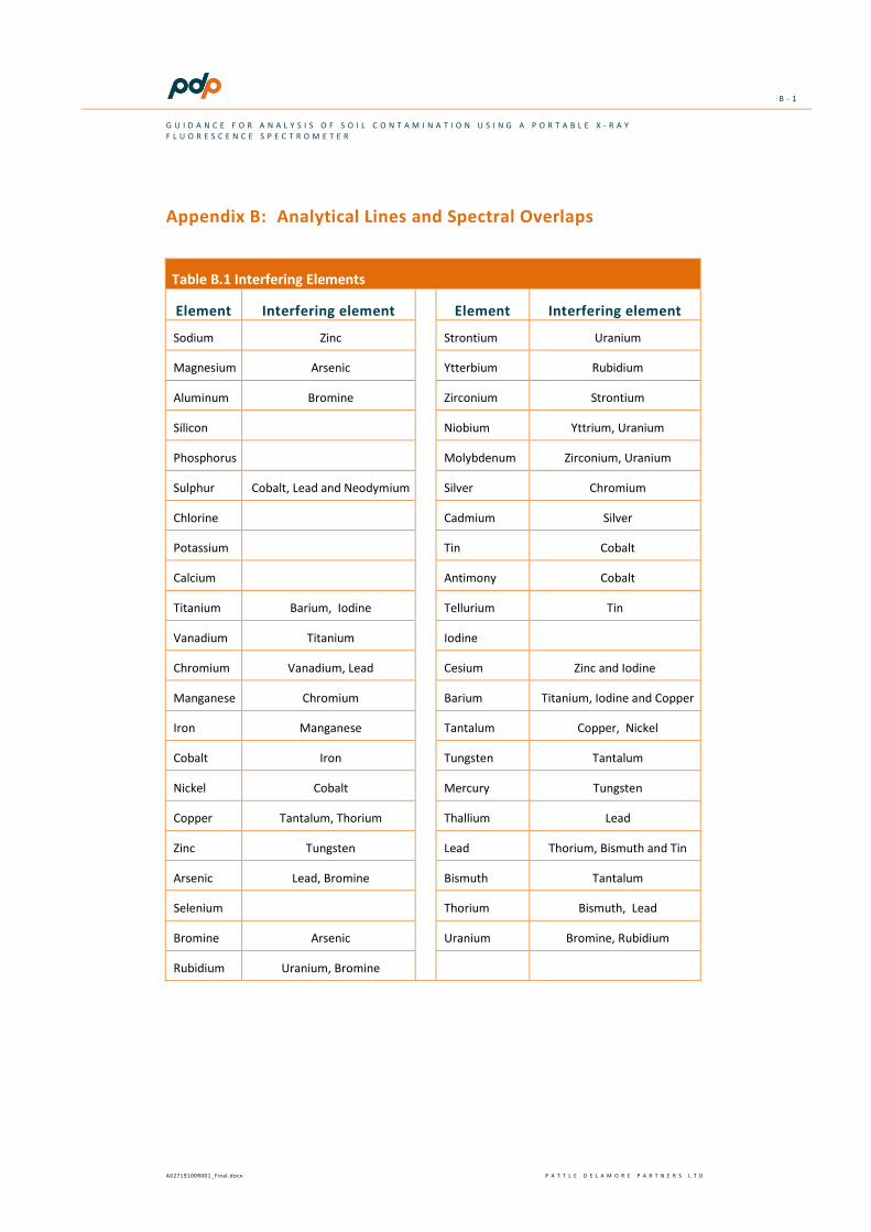
B - 1



Appendix B: Analytical Lines and Spectral Overlaps

Table B.1 Interfering Elements

Element Interfering element Element Interfering element

Sodium Zinc Strontium Uranium

Magnesium Arsenic Ytterbium Rubidium

Aluminum Bromine Zirconium Strontium

Silicon Niobium Yttrium, Uranium

Phosphorus Molybdenum Zirconium, Uranium

Sulphur Cobalt, Lead and Neodymium Silver Chromium

Chlorine Cadmium Silver

Potassium Tin Cobalt

Calcium Antimony Cobalt

Titanium Barium, Iodine Tellurium Tin

Vanadium Titanium Iodine

Chromium Vanadium, Lead Cesium Zinc and Iodine

Manganese Chromium Barium Titanium, Iodine and Copper

Iron Manganese Tantalum Copper, Nickel

Cobalt Iron Tungsten Tantalum

Nickel Cobalt Mercury Tungsten

Copper Tantalum, Thorium Thallium Lead

Zinc Tungsten Lead Thorium, Bismuth and Tin

Arsenic Lead, Bromine Bismuth Tantalum

Selenium Thorium Bismuth, Lead

Bromine Arsenic Uranium Bromine, Rubidium

Rubidium Uranium, Bromine


Appendix C

Detectio

n Lim

its for FP

‐XRF fo

r Selected

Elemen

ts

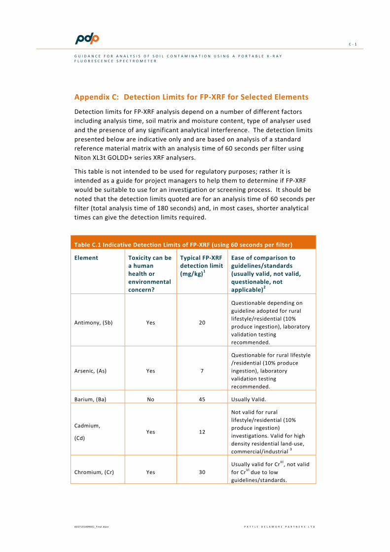
C - 1



Appendix C: Detection Limits for FP-XRF for Selected Elements

Detection limits for FP-XRF analysis depend on a number of different factors including analysis time, soil matrix and moisture content, type of analyser used and the presence of any significant analytical interference. The detection limits presented below are indicative only and are based on analysis of a standard reference material matrix with an analysis time of 60 seconds per filter using Niton XL3t GOLDD+ series XRF analysers.

This table is not intended to be used for regulatory purposes; rather it is intended as a guide for project managers to help them to determine if FP-XRF would be suitable to use for an investigation or screening process. It should be noted that the detection limits quoted are for an analysis time of 60 seconds per filter (total analysis time of 180 seconds) and, in most cases, shorter analytical times can give the detection limits required.

Table C.1 Indicative Detection Limits of FP-XRF (using 60 seconds per filter)

Element Toxicity can be a human health or environmental concern?

Typical FP-XRF detection limit (mg/kg)1

Ease of comparison to guidelines/standards (usually valid, not valid, questionable, not applicable)2

Antimony, (Sb) Yes 20

Questionable depending on guideline adopted for rural lifestyle/residential (10% produce ingestion), laboratory validation testing recommended.

Arsenic, (As) Yes 7

Questionable for rural lifestyle /residential (10% produce ingestion), laboratory validation testing recommended.

Barium, (Ba) No 45 Usually Valid.

Cadmium,

(Cd) Yes 12

Not valid for rural lifestyle/residential (10% produce ingestion) investigations. Valid for high density residential land-use, commercial/industrial 3

Chromium, (Cr) Yes 30 Usually valid for CrIII, not valid for CrVI due to low guidelines/standards.

C - 2



Table C.1 Indicative Detection Limits of FP-XRF (using 60 seconds per filter)

Element Toxicity can be a human health or environmental concern?

Typical FP-XRF detection limit (mg/kg)1

Ease of comparison to guidelines/standards (usually valid, not valid, questionable, not applicable)2

Cobalt, (Co) Yes 90

Not valid for rural lifestyle /residential (10% produce ingestion), laboratory validation testing recommended

Copper, (Cu) Yes 15 Usually valid

Iron, (Fe) No 25 Usually valid

Lead, (Pb) Yes 8 Usually valid

Manganese, (Mn) No 65 Usually valid

Mercury, (Hg) Yes 9

Usually valid for inorganic mercury. Not valid for methyl mercury.

Molybdenum, (Mo)

No 3 Not applicable

Nickel, (Ni) Yes 30 Usually valid

Potassium, (K) No 150 Not applicable

Selenium, (Se) Yes 4 Usually valid

Sulphur, (S) No 350 Not applicable

Tin, (Sn) Yes 20 Usually valid

Vanadium, (V) Yes 60 Usually valid

Uranium, (U) Yes 7 Usually valid

Zinc, (Zn) Yes 12 Usually valid

Notes. 1. Detection limits determined in accordance with Definition and Procedures for the Determination of the

Method Detection Limit. 40 CFR, Part 136, Appendix B. Revision 1.11. U.S. Environmental Protection Agency.

2. Based upon guideline values/soil standards for protection of human health at the time of writing. Guideline values can change and it is important to verify guidelines values before determining if FP-XRF will be a valid tool for the particular project.

3. In some New Zealand soils the XRF appears to give erroneous high results although these results do not appear to be associated with any known interferences.


Appendix D

Flow Charts O

utlin

ing th

e Processes o

f XRF Field

Analyses o

f Soils

D - 1



Appendix D: Flow Charts Outlining the Processes of XRF Field Analyses of Soils

P A T T L E D E L A M O R E P A R T N E R S L T D

Figure D-1 : Initial prechecks before undertaking XRF investigations

G U I D A N C E F O R A N A L Y S I S O F S O I L C O N T A M I N A T I O N U S I N G A P O R T A B L E X - R A Y F L U O R E S C E N C E S P E C T R O M E T E R ( X R F )

Conduct visual inspection of the instrument to confirm integrity of window

Clean XRF window as necessary

Switch instrument on and allow instrument sufficient time to warm up (in

accordance with manufacturers instructions)

Select suitable soil matrix programme based on expected soil type and

concentration range

Analyse blank sample

Passed energy calibration check?Stop XRF

Possible fault in instrument

Did blank sample pass project’s QA criteria?

Select appropriate CRM for the site and analysis CRM

Did CRM analysis meet project’s QA requirements for

the target elements?

Stop XRFXRF may be need to be recalibrated

No

Yes

Yes

No

No

Yes

Instrument is OK to begin XRF Survey


Figure D-2 : Outline of in-situ analysis of soil sample using field-portable XRF


Check functionality of instrument in accordance with Figure D-1/Section 7.2.2

Select suitable sampling locations

Check that window is clean before analysing next sample

Remove debris (e.g. leaves and gravels)

If covered in grass, remove grass and roots (usually remove upper 20 to 50 mm

of soil)

When ready to measure, level surface area and pack down soil

Loosen soil to a depth of 15 to 25 mm over measurement area

XRF soils for at least 30 to 60 seconds (may require longer to achieve project

detection limits)

No

Is soil moist? Allow to dry for 1 to 2 hoursYes


Figure D-3 : Outline of qualitative grab analysis of soil sample using field-portable XRF


Check functionality of instrument in accordance with Figure D-1/Section 7.2.2


Check if window is clean before analysing next sample

Remove debris (e.g. leaves and gravels)

If covered in grass, remove grass and roots (usually remove upper 20 to 50 mm

of soil)

Place sample inside labelled plastic bag

Homogenise sample by either kneading sample (for clay soils) or turning bag end

over end (for silty & sandy soils)

Create smooth flat surface on sample. Fold bag over tightly to enclose sample

Sample thickness should be no more than 10 mm thick

Air dry sample in open tray (if necessary)

XRF soils for at least 30 to 60 seconds (may require longer if to achieve project

detection limits)


Figure D-4 : Outline of semi-quantitative analysis of soil sample using field-portable XRF


Check functionality of instrument as outlined in Figure D-1/Section 7.2.2


Is the sample dry?Dry sample

Is the sample suitable for sieving?

Sieve through 2 mm sieve

Yes

No

YesRemove gravel and twigs from sample

if requiredNo

Homogenise sample

See Figure D-5

Is RSD of replicates sufficiently low?

Will additional sample preparation improve RSD?

Adjust DQOs to screening survey or send samples for lab analysisContinue with survey

Yes

No

No

Yes


Figure D-5 : Steps in assessing homogeneity of sample for semi-quantitative analysis


Obtain soil sample

Mix sample thoroughly and place in re-sealable bag

Create a smooth surface for analysis

Perform at least 8 analyses of the sample

Is the %RSD of target analytes less than 30%?

No further sample preparation required

Undertake sample preparation (see Section 7.1.2.2) and undertake further

analysis

Is the %RSD of target analytes less than 30%?

No further sample preparation required

Sample not suitable for semi-quantitative analysis

Consider undertaking screening level investigation or send samples to lab

Yes

No

Yes

No


Appendix E

Calcu

lating U

ncertain

ty of M

easurem

ent

E - 1



Appendix E: Calculating Uncertainty of Measurement

Measurements of contaminant concentrations are only ever estimates of the “true” value of that concentration because they are subject to uncertainties arising from statistical errors in the measurement process (i.e. sampling, sample preparation and the analysis of the sample). This is true for all types of analysis of soils whether undertaken in the field using a XRF or in a certified analytical laboratory. A result of any analysis is therefore only really complete when it is accompanied by a quantitative statement of the uncertainty. Uncertainty estimates are required for a defensible assessment of the fitness of purpose of the dataset to meet the investigation objectives.

The uncertainty of measurement of soil samples consists of several different components. However, it is beyond the scope of this guidance to discuss the various sources of uncertainty in sampling. Further information may be found in Ramsey and Ellison (2007) and US EPA (1992).

There are two main approaches to determining the uncertainty of measurement; the empirical approach20 and the modelling approach21.

For most contaminated site investigations the empirical approach is used. This approach generally uses statistical methods based upon the replicated measurements of samples (Type A evaluation of uncertainty) or uses scientific judgement to estimate uncertainty (Type B evaluation of uncertainty).

A Type A evaluation of uncertainty may be based on any valid statistic method for treating data. This could include the following techniques:

1. A calculation of 95% interval using a standard error of the mean (SEM) approach modified using a t-distribution for a dataset with less than 100 data points. This approach is relatively simple and can be used with datasets which are normally distributed or can be transformed into a normal distribution (i.e. by undertaking a log transformation). For a population which is not normally distributed then it is recommended that a one-sided Chebyshev theorem is used22.

2. A robust ANOVA approach on the duplicate samples to calculate relative error associated with sampling and analysis and sampling bias determined using linear FREML (functional relationship estimation by maximum likelihood). This approach is technically superior to the SEM

20 Empirical approach is also referred to as being the experimental, retrospective or top down approaches. 21 Modelling approach is also referred to as the theoretical, predictive, or bottom up approach, and uses sampling theory developed by Pierre Gy to predict the variance in the sample. 22 The US EPA’S ProUCL public domain software can be used to calculate both standard error of the mean and one sided Chebyshev theorem approaches.

E - 2



approach but it requires a high degree of statistical knowledge and specialised software. This method is discussed in Boon and Ramsey (2010).

3. Geo-statistical methods using semi-variograms or modelling the sources of the error using Gy sampling theory. These approaches require specialised statistical knowledge and software. Also, if geo-statistical techniques are to be used this needs to be identified at the beginning of the project so that an appropriate sampling plan for the site can be developed. Geo-statistical techniques are more appropriate for a large dataset (over 50 samples).

In all cases the aim is to characterise the reliability and representativeness of measurements, to enable development and support of defensible statements about the actual contaminant distribution at the site. Before using any statistical technique it is important to answer two fundamental questions:

• What is the distribution of the data?

• What is the desired confidence level required from the statistical test?

Understanding the distribution of the data is necessary to select the appropriate statistical technique. All datasets which are intended to be subject to a statistical test should first be analysed to assess the distribution of the data. Readily available free software packages such as the US EPA’s ProUCL can be utilised to undertake such analyses.

With respect to the desired confidence level, most statistical tests are conducted using a 95% confidence interval. However, this level of confidence is not always required to meet the project’s objectives. If a 95% confidence level is not used, then justification should be provided as to why another confidence level (e.g. 80% or 90%) is appropriate.

Type B evaluations are based on scientific judgement using all the information available (NIST, 1994; ISO/IEC 98-2:2008). Type B evaluations include:

• Uncertainties calculated from previously measured data using a Type A technique (must be for a site with similar soil type and chemical composition).

• Empirical methods outlined in prEN 16424 (2012).

Type B evaluations are more suited for investigations where real time assessment of the data is required and it is not possible to undertake an assessment of the data in the field (such as on-site remediation), or screening level assessments to identify the presence or absence of hotspots.


Appendix F

Data C

omparab

ility Checks

F - 1



Appendix F: Data Comparability Checks

Data comparability checks are needed to verify that the data from semi-quantitative FP-XRF investigations are comparable with traditional sampling techniques. The US EPA Method 6200 (US EPA, 1998) recommends that one in every twenty samples is sent to the laboratory for confirmatory analysis. In reality, at least three samples are required to undertake any kind of regression analysis. Samples which are used for data comparability verification should be within the decision-making range.23

Comparability analysis is typically undertaken using a linear regression analysis to measure “the goodness of fit”. If the correlation coefficient (r) is between 0.9 and 1.0 then according to US EPA (1998) “the data could potentially meet definitive level data criteria” or in other words, the data may be used to make decisions as to whether the results are above or below the relevant threshold value.

A conventional regression analysis can give misleading results because it assumes no error in the x-axis, which implies the laboratory analysis is without sampling error, which will not be true. Laboratory measurements generally have better accuracy and precision than field XRF and, as an approximation, standard regression will frequently suffice. However, if laboratory error is a concern, Total Least Squares regression is an approach which allows for presence of errors in both sets of measurements (x and y).

One of the most common problems with application of regression equations is use of inappropriately distributed data, e.g. data with outliers.

Figure F-1 illustrates how outliers can influence the regression. In the top graph the dataset contains two very high results for lead (approximately 6000 and 8000 ppm), while most of the lead measurements are less than 400 ppm. Including the two high values in the linear regression analysis gives an R2 value of 0.95 (equivalent to an r of 0.97).

This is artificially high and is not a valid result, because it is caused by the data approximating a two-point line. It is important to appreciate that the correlation coefficient values are valid only if the underlying dataset is approximately normally distributed. Many environmental datasets are skewed (sometimes approximating a log-normal distribution).

One approach to solving this problem is to take log values of the results to see whether the points become reasonably evenly distributed along the line.

23 Samples which are below the XRF detection limit or have very high concentrations should not be submitted for data comparability checks. Ideally, there should be an equal number of samples above and below the decision value and the concentration of the element of concern should be within an order of magnitude of the decision value.

F - 2



Another approach is to treat the high and low values as being drawn from distinct populations when making comparisons between analysis methods. On contaminated sites, three or more populations may exist – for example representing the clean areas, areas with modest amounts of contamination, and the highly contaminated “hotspots”.

Figure F-1. Example of how unbalanced data set can affect the regression co-efficient

Examination of the data in Figure F-1 shows three additional problems. The first is that the y-intercept of the graph is 200 ppm. This suggests that the XRF data has a systematic bias of 200 ppm, which would be unacceptable if the purpose was risk assessment for a residential scenario, as the soil contaminant standard for lead is close to 200 ppm.

The second problem is that the slope of the graph is 0.54, which is not close to unity. The third problem which can be seen by examining the scatterplot is that it appears that the dataset below 400 ppm has a significantly different slope to that drawn by the regression analysis (i.e. the regression analysis does not

F - 3



describe the dataset below 400 ppm very well, which is the part of the dataset relevant for making decisions about lead).

When the data is re-analysed using the data which has concentrations of less than 400 ppm, the R2 value regression coefficient drops to 0.85 (equivalent to an r of 0.92) which is lower than previously but just within the US EPA criteria for data comparability of between 0.9 and 1.0.

A more robust technique to assess data comparability, recommended by the US EPA (US EPA, 2010), is to undertake duplicate measurements on both the FP-XRF and the laboratory measurements of the samples. The results of the duplicate analysis are then plotted on the same regression curve (i.e. Lab 1 versus Lab 2 and XRF1 versus XRF2) so that there are two lines on the one graph.

If the XRF1/XRF2 regression line falls within the calculated laboratory 95% confidence interval then the XRF dataset is comparable to the laboratory dataset – see Figure F-2. In Figure F-2, the XRF data is the blue crosses and the ICP data is the black circles.

The XRF-XRF duplicate regression line falls within the ICP 95% confidence interval (dashed red lines). This means that the XRF data set is comparable to the ICP dataset. In addition to undertaking a regression evaluation the slope and intercept of the XRF data should be also inspected. The y-intercept of the XRF data should be close to zero (a high y-intercept value may indicate the presence of a systematic error or a calibration problem with the instrument). The slope of the XRF data should be close to one.

This technique should be considered for use on sites where sample heterogeneity is known or suspected to occur (e.g. lead paint in soils, sites impacted by aerial deposition of particulates (abrasive blasting) and sites impacted by mining activities).


Appendix G

Summary X

RF R

eport C

hecklist

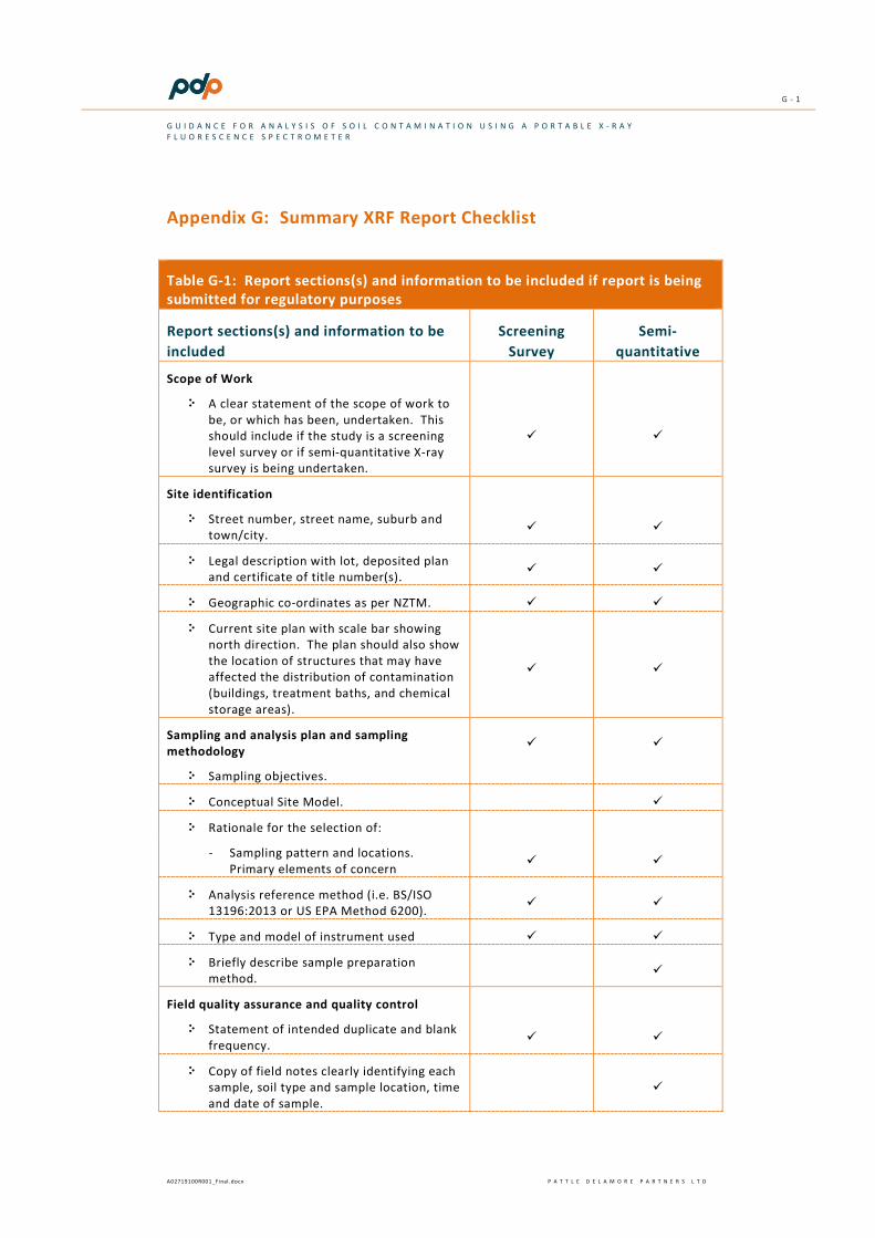
G - 1



Appendix G: Summary XRF Report Checklist

Table G-1: Report sections(s) and information to be included if report is being submitted for regulatory purposes

Report sections(s) and information to be included

Screening Survey

Semi-quantitative

Scope of Work

• A clear statement of the scope of work to be, or which has been, undertaken. This should include if the study is a screening level survey or if semi-quantitative X-ray survey is being undertaken.

Site identification

• Street number, street name, suburb and town/city.

• Legal description with lot, deposited plan and certificate of title number(s).

• Geographic co-ordinates as per NZTM.

• Current site plan with scale bar showing north direction. The plan should also show the location of structures that may have affected the distribution of contamination (buildings, treatment baths, and chemical storage areas).

Sampling and analysis plan and sampling methodology

• Sampling objectives.

• Conceptual Site Model.

• Rationale for the selection of:

- Sampling pattern and locations. Primary elements of concern

• Analysis reference method (i.e. BS/ISO 13196:2013 or US EPA Method 6200).

• Type and model of instrument used

• Briefly describe sample preparation method.

Field quality assurance and quality control

• Statement of intended duplicate and blank frequency.

• Copy of field notes clearly identifying each sample, soil type and sample location, time and date of sample.

G - 2



Table G-1: Report sections(s) and information to be included if report is being submitted for regulatory purposes

Report sections(s) and information to be included

Screening Survey

Semi-quantitative

• Decontamination procedure between samples.

• Sample splitting techniques and field instrument calibrations (where used).

• Limit of detections for various elements under consideration in the survey.

QA/QC data evaluation

• Evaluation of all field QA/QC information listed above against stated DQOs, including:

- Documentation and data completeness;

- Precision and accuracy;

- Limitations in the reliability of the data;

- RPD in precision and accuracy checks;

- Data compatibility.

Results

• Site plan showing all the sampling locations, giving sample identification and sample depth.

• Copy of raw XRF results together with sample ID, time and date of sample, analysis time.

• Uncertainty of measurements

• Rationale for selecting technique for measuring uncertainty.

Conclusions and recommendations

• A brief summary of all relevant findings.

• Assumptions used in making conclusions.

• Extent of uncertainty in the results.

• A statement detailing all limitations of the investigation including potential impact of inferences.

• Recommendations for further work, if appropriate.

guidance for analysis of soil contamination using a ... · sampling locations for site...

Documents