WP/16/176

Growing Apart, Losing Trust? The Impact of Inequality on Social Capital

by Eric D. Gould and Alexander Hijzen

IMF Working Papers describe research in progress by the author(s) and are published to elicit comments and to encourage debate. The views expressed in IMF Working Papers are those of the author(s) and do not necessarily represent the views of the IMF, its Executive Board, or IMF management.

© 2016 International Monetary Fund WP/16/176

IMF Working Paper

Research Department

Growing Apart, Losing Trust? The Impact of Inequality on Social Capital1

Prepared by Eric D. Gould and Alexander Hijzen

Authorized for distribution by Romain Duval

August 2016

Abstract

There is a widespread perception that trust and social capital have declined in United States as well as other advanced economies, while income inequality has tended to increase. While previous research has noted that measured trust declines as individuals become less similar to one another, this paper examines whether the downward trend in social capital is responding to the increasing gaps in income. The analysis uses data from the American National Election Survey (ANES) for the United States, and the European Social Survey (ESS) for Europe. Our analysis for the United States exploits variation across states and over time (1980-2010), while our analysis of the ESS utilizes variation across European countries and over time (2002-2012). The results provide robust evidence that overall inequality lowers an individual’s sense of trust in others in the United States as well as in other advanced economies. These effects mainly stem from residual inequality, which may be more closely associated with the notion of fairness, as well as inequality in the bottom of the distribution. Since trust has been linked to economic growth and development in the existing literature, these findings suggest an important, indirect way through which inequality affects macro-economic performance.

JEL Classification Numbers: H00, J31, Z1

Keywords: social capital, earnings, redistribution

Author’s E-Mail Address: eric.gould@mail.huji.ac.il; alexander.hijzen@oecd.org

1 Much of the work for this paper was conducted when the authors were visiting the International Monetary Fund. The authors are grateful to the International Monetary Fund for its hospitality and would like to thank Romain Duval, Jonathan Ostry, and seminar participants at the IMF for useful discussions, comments, and suggestions. The views expressed in this paper are those of the authors and cannot be attributed to the IMF, the OECD, or their member countries. Also, the authors are responsible for any remaining errors.

IMF Working Papers describe research in progress by the author(s) and are published to elicit comments and to encourage debate. The views expressed in IMF Working Papers are those of the author(s) and do not necessarily represent the views of the IMF, its Executive Board, or IMF management.

3 Contents Page

I. INTRODUCTION ____________________________________________________________________________ 5 

II. DATA _______________________________________________________________________________________ 9 A. The ANES Data for the analysis of the United States __________________________________________ 10 B. The EES Data for the Analysis of Europe _______________________________________________________ 14 

III. EMPIRICAL STRATEGY __________________________________________________________________ 15 

IV. ANALYSIS OF ANES FOR THE UNITED STATES ________________________________________ 16 

V. ANALYSIS FOR EUROPEAN COUNTRIES ________________________________________________ 19 

VI. CONCLUSION ___________________________________________________________________________ 21 

REFERENCES_________________________________________________________________________________23 FIGURES 1. Trust has declined sharply in the United States__________________________________________ 6 2. The 90/10 ratio of hourly earnings over time in the U.S. ________________________________12 3. Change in the college premium in the united states____________________________________ 13 4. Residual inequality measures int eh united states_______________________________________ 13 5. Residual inequality by state in the u.s.:1980-2010_______________________________________ 14

TABLES 1. ANES Summary Statistics - Means of Demographic Variables___________________________26 2. ANES Summary Statistics - Means of Trust and Other Social Capital Variables_________ 27 3. ANES Trends in "Trust People" in the United States from 1980-2000___________________ 28 4. ANES Trends in Trust and Other Social Capital Variables________________________________29 5. Summary Statistics of Demographics and Social Capital Variables in the ESS Sample__ 30 6. Summary Statistics of Inequality Measures in the ESS Sample__________________________ 31 7. ESS Trends in "Trust People" in Europe from 2002-2014________________________________ 32 8. ANES Analysis of Inequality and Trust with Robustness Checks to Control Variables

20-45 Year Olds__________________________________________________________________________33 9. ANES Analysis of Inequality and Trust with Robustness Checks to Control Variables

46-65 Year Olds__________________________________________________________________________34 10. ANES Analysis of Overall Inequality Measures and Social Capital Outcomes

(Ages 20-45)_____________________________________________________________________________ 35 11. ANES Analysis of Inequality at the Bottom End and Social Capital Outcomes

(Ages 20-45)_____________________________________________________________________________ 36

4

12. ANES Analysis of Inequality at the Top End and Social Capital Outcomes

(Ages 20-45)_____________________________________________________________________________ 37 13. ANES Analysis of Social Capital with Multiple Inequality Variables Together___________ 38 14. ANES Analysis of Residual 50/10 Inequality on Social Capital by Subgroups___________ 39 15. ANES Analysis of Residual 90/50 Inequality on Social Capital by Subgroups____________ 40 16. ESS Analysis of Inequality and Trust with Robustness Checks____________________________41 17. ESS Analysis of Inequality on Various Social Capital Measures for Ages 25-65__________ 42 18. ESS Analysis of Inequality on Various Social Capital Measures for Ages 25-65__________ 43 19. ESS Analysis of 90/10 Inequality on Various Social Capital Measures within Subgroups

for Ages 25-65___________________________________________________________________________ 44 20. ESS Analysis of 50/10 Inequality on Various Social Capital Measures within Subgroups

for Ages 25-65___________________________________________________________________________ 45 21. ESS Analysis of 90/50 Inequality on Various Social Capital Measures within Subgroups

for Ages 25-65___________________________________________________________________________ 46

5

I. INTRODUCTION

There has been a sharp decline in the extent to which individuals trust one another, and other social capital indicators, over the past forty years in the United States. At the same time, income inequality has increased in the United States and many advanced countries. This paper investigates whether the two trends are related to one another. Looking at the link between these two phenomena is motivated by the literature showing that individuals have less trust in people that are dissimilar to them. If this finding extends to differences between people in their income, the increasing inequality trend witnessed in many advanced countries may have had an important influence on aggregate trust levels. Given that a country’s overall level of trust has been found to be an important determinant of growth and development, sorting out the relationship between inequality and trust is necessary to see if income inequality has an indirect influence on macro-performance through its effect on trust between individuals.2 The standard “generalized trust” variable contained in many surveys refers to how much a person trusts unspecified persons. That is, trust does not refer to how much someone trusts their personal friends or family members. Generalized trust is typically considered a key component of social capital, which refers to the features of social life “that enable participants to act together more effectively to pursue shared objectives” (Putnam, 1995). Trust is typically measured in surveys by the question: “Generally speaking, would you say that most people can be trusted; or that you can’t be too careful when dealing with others?” Possible answers are: “Most people can be trusted” or “Can’t be too careful”. Since the early 1970s, the share of persons in the United States responding that most people can be trusted has declined from about fifty percent to thirty-three percent by 2010 (Figure 1). When controlling for changes in the demographic composition of the US population over this period in terms of education and age, the decline in generalised trust is even more pronounced. The decline in trust may have important implications for economic performance (see Guiso et al., 2006; Algan and Cahuc, 2013; Alesina and Giuliano, 2016, for reviews). First of all, trust facilitates economic interactions in the private sphere by reducing transaction costs and by mitigating principal-agent problems. Trust has been shown to promote economic growth generally (Knack and Keefer, 1997; Tabellini, 2010, Algan and Cahuc, 2010) as well as specific drivers of economic growth such as international trade (Cingano and Pinotti, 2016),

2 The model in Galor and Zeira (1993) shows how inequality adversely affects growth in the presence of credit constraints. A number of recent papers have suggested that inequality reduces growth (Cingano, 2014; Ostry et al., 2014; Deblas-Norris et al., 2015).

6

financial development (Guiso et al., 2004, 2008, 2009), innovation, entrepreneurship, and firm productivity (Bloom et al., 2012). Trust can also promote cooperation in the public sphere by reducing collective action problems related to the provision of public goods and by enhancing the overall quality of public institutions (La Porta et al., 1999; Tabellini, 2008; Nannicini et al., 2012).

Economic inequality is often seen as an important determinant of trust.3 Both inequality of opportunities and inequality in outcomes may be important. To the extent that economic disparities derive from personal connections or mere luck rather than individual merit, they may lower a person’s sense of fairness, and therefore, trust in others and government. This argument relates to the role of inequality of opportunities and the scope for social mobility (Putnam, 2015).4 In addition, if economic outcomes determine values, and trust depends on having common values, larger income gaps will reduce a person’s general sense of trust by increasing disparities in values. This is a specific interpretation of the more general statement

3 See also Jordahl (2007) for a discussion.

4 Alesina, Cozzi and Mantovan (2012) provide a dynamic model that builds on a similar reasoning to explain persistent differences in attitudes to inequality and redistribution in Europe and the United States. They argue that the greater importance of inheritance in Europe and merit in the United States for the distribution of wealth at the start of the industrial revolution explain the relatively weak tolerance for inequality and strong support for redistribution in Europe.

.2.3

.4.5

.6

1970 1980 1990 2000 2010year

actual adjusted

Actual: actual share of working-age population responding that most people can be trustedAdjusted: composition-adjusted share of working-age population responding that most people can be trustedSource: General Social Survey, 1972-2012

share of working-age population responding that most people can be trustedFigure 1: Trust has declined sharply in the United States

7

that “familiarity breeds trust” (Coleman, 1990).5 According to this argument, inequality in outcomes provides an indication of the degree of social stratification in society. Several studies have shown that there is a strong relationship between trust and inequality using cross-sectional variation across regions in the United States (Alesina and La Ferrera, 2002; Rothstein and Uslaner, 2005; Twenge et al., 2014; Tesei, 2015)6 as well as across countries around the world (Zak and Knack, 2001). However, systematic evidence on the causal relationship between inequality and trust remains rather limited. Also, little attention has been devoted to the underlying mechanisms or the relevance of specific aspects of inequality. Using individual panel data for Sweden during the period 1994-1998, Gustavsson and Jordahl (2007) exploit variation over those years in inequality across regions and find that household inequality reduces trust, especially when it is concentrated in the bottom of the distribution. Moreover, they find that the effect is stronger in terms of inequality of disposable income rather than market income, and also for people who favor more redistribution. These findings suggest that in Sweden redistribution can help to alleviate the adverse effect of inequality on trust. Using variation over time and across countries with the World Values Survey, Barrone and Mocetti (2016) find that inequality reduces trust, even after controlling for country fixed effects, but only among advanced economies. Moreover, in contrast to Gustavsson and Jordahl (2007), they find that the negative relationship between inequality and trust is driven by inequality at the top end of the distribution. They also provide suggestive evidence that the impact of trust on inequality is smaller when there is more inter-generational mobility. This paper contributes to the small, existing literature on the relationship between inequality and social capital in several ways. Although our main focus is on the relationship between inequality and trust, we also examine other social capital variables such as an individual’s views about: the helpfulness of others, whether others are fair, trust in government, views about redistribution, and life satisfaction. These additional outcomes serve as a useful robustness check for the relationship between inequality and trust, but also allow us to glean insights into the possible mechanisms. In addition, we examine the relationship between trust and inequality by using several different dimensions and components of inequality. For example, we analyse inequality in individual wages using the ratio of the 90th to the 10th percentile of personal wage income.

5 A number of studies have analysed the role of ethnic diversity (Alesina and La Ferrera, 2002; Putnam, 2007; Dinesen and Sonderkov, 2015).

6 Alesina and La Ferrera (2002) and Tesei (2015) use variation across MSAs for multiple years while controlling for state fixed effects. Their findings appear to be mainly driven by the cross-sectional variation in the data. Tesei (2015) find that this relationship is sensitive to the specification.

8

We further decompose this measure into the component that is due to the large returns to investments in education (the return to education) and the part that is unexplained by differences in age, education, industry, and occupation (“residual inequality”). This residual inequality measure is further decomposed into inequality at the top (the ratio of the 90th percentile to the median of the residual wage distribution), and to inequality at the bottom (the ratio of the median to the 10th percentile). In addition, we use alternative measures of household income inequality such as the gini, the poverty rate, the poverty gap, and the income shares of the top 1 percent, the top 5 percent, and the top 10 percent. Furthermore, similar to recent papers, we exploit geographic variation over time to control for fixed-factors which may be determining inequality and trust, but this study is the first to do so for the United States, as well as European countries with the European Social Survey (ESS). To shed light on possible mechanisms behind a relationship between inequality and trust, we explore whether the results differ across groups defined by education, age, income, and gender. The results provide robust evidence that overall inequality substantially lowers an individual’s sense of trust in others in the United States as well as in other advanced economies. The results for the United States indicate that the increase in inequality between 1980 and 2000 explains forty-four percent of the observed decline in trust. Although inequality at the top of the distribution is found to be significant in many specifications, the negative relationship between inequality and trust in the United States appears to be more robust for inequality at the bottom of the distribution. In addition, the effect is stronger for “residual inequality” (i.e. inequality within age, education, industry, and occupation groups) versus overall inequality, younger (ages 20-45) versus older people (46-65), and for individuals that are the most adversely affected by inequality at the bottom of the distribution – individuals that are less educated or in the bottom third of the income distribution. Similar findings are obtained for “trust in government” and other social capital variables, including concerns about “unequal chances.” But, there is no evidence that inequality increases the demand for greater redistribution in the United States. In addition, the return to education has no effect on trust, which may indicate that inequality between groups of people stemming from personal decisions and human capital investments does not undermine trust, but increasing inequality among similar people may be regarded as unfair, and thus, reduce trust in others. Similar findings are found using variation across European countries with the ESS, suggesting that the adverse impact of inequality on trust extends beyond the United States to advanced economies with different institutional settings. The one notable difference is that the effect of inequality on trust seems to be more general in the sense of coming from the top and bottom parts of the distribution, and affecting people similarly across age and education categories. In both the United States and Europe, there is no evidence that inequality at the very top of the distribution (the top 1 percent or top 10 percent) is affecting trust levels,

9

however, this type of high end inequality in Europe does seem to increase the desire for government to reduce income gaps in society. A causal interpretation of our findings is supported by the many robustness checks, and by investigating whether the estimates are robust to the inclusion and exclusion of a wide variety of personal and geographic area (state or country) characteristics. For example, our main finding that inequality from the bottom of the distribution affects trust is found when only basic controls are included in the specification (age, education, gender) and when additional controls are included like race, religion, income, employment status, and geographic area measures for the mean wage, demographic composition, crime rates, and immigrant concentration. The robustness of this effect to the inclusion and exclusion of all these additional control variables supports the identifying assumption that the results would not be sensitive to the inclusion of additional, omitted determinants of a person’s views about trust in others. In addition, when several inequality measures from different parts of the distribution are included in one specification for the United States, inequality at the bottom end remains statistically significant, in contrast with the others. This result is notable because the inclusion of inequality at the top of the distribution implicitly controls for many factors that are affecting both inequality and trust. In the analysis of Europe, inequalities at both ends are significant when included in the same specification. Although there are some differences in the results for the United States and Europe, the overall pattern suggests that the role of inequality on trust in others is not limited to the United States, but holds across advanced economies. Given the rise in inequality in many advanced economies, and the importance of trust for macro-performance documented in the literature, the results suggest an important, albeit indirect, way through which rising inequality could be affecting a country’s growth and development. The remainder of the paper is structured as follows. The next section describes the data and the trends from the American National Election Survey (ANES) and the European Social Survey (ESS). Section 3 presents the empirical framework. The results for the United States are in Section 4, while the European analysis is presented in Section 5. Section 6 summarizes our findings and concludes.

II. DATA

In order to explore whether inequality affects measures of trust, attitudes towards redistribution, and other social capital indicators, two main sources of data are used in distinct analyses – one for the United States and one for Europe. For the United States, we use the American National Election Surveys (ANES) for election years 1980-2012, and the analysis of Europe is based on the European Social Survey (ESS) from 2002-2014.

10

A. The ANES Data for the analysis of the United States

The ANES contains variables on trust and other social capital indicators, as well as information on state of residence, which allows us to exploit geographic variation across states and over time (1980-2010). Information from the ANES is matched to state-level measures of inequality, computed from the Census for every ten years from 1980 to 2010. Since the ANES is conducted during election years, respondents in the ANES were matched to the state-level inequality measure in the closest census year. Throughout the analysis, we use the term “year” to refer to the census year, which are matched to the ANES survey years as follows: the 1980 Census is matched to the ANES surveys from 1976, 1978, 1980, and 1982; the 1990 Census is matched to the ANES surveys from 1988, 1990, and 1992; the 2000 Census is matched to the ANES surveys from 1998, 2000, and 2002; and the 2010 Census is matched to the ANES surveys from 2008 and 2012. The sample sizes for each variable vary across Census years, mainly because of differences in the number of rounds of the ANES survey used, and the ANES surveys did not always ask the same questions in each round. Table 1 presents summary statistics of the main demographic variables in the American National Election Survey (ANES). In addition to age, gender, and education, the surveys contain information on ethnicity, religion, marital status, employment status, and which third of the family income distribution the respondent belongs to. Table 2 displays summary statistics for the social capital outcomes and other views of respondents in the ANES. Similar to other studies, the trust outcome is measured as a dummy variable for whether the respondent indicates that “most people can be trusted” versus “you can’t be too careful.” The ANES also has an indicator for “fairness” – defined as responding that “people would try to be fair” as opposed to “people will take advantage of others.” In addition, “people are helpful” is an indicator for responding that “people try to be helpful” relative to “people just look out for themselves.” Since all three relate to the goodwill of others, we created a summary index using factor analysis which turns out to give nearly equal weights to all three variables. The means for all of these social trust measures are given in Table 2. Table 2 also shows the means for indicators of whether the respondent trusts government to benefit all, and whether the person trusts government to do right. The ANES uses these and other variables to create an index for how much the respondent generally trusts government, which ranges from 0 to 100 with higher values indicating higher levels of trust. Finally, Table 2 shows the means for measures which capture how much the person is bothered by inequality (a scale from 1 to 5 which increases in how much the respondent thinks unequal chances are a problem), a measure for how much the person wants to increase spending on the poor (0 = decrease; 1 = stay the same; 2 = increase spending), and an indicator for whether the person believes that “government should do more” relative to “less

11

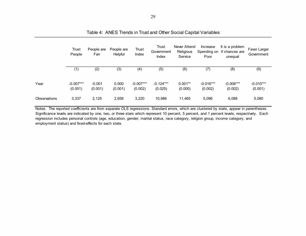
government is better.” Although the means over time in Table 2 do not show a strong downward trend in trust, Table 3 reports regressions of the trust measure on a linear time trend variable. The first column contains no other controls and uses a sample of 20-45 year olds, and the trend is significantly downward. Adding controls for age and gender yield a similar time trend, but adding controls for education, marital status, religion, family income, employment status, and state fixed-effects yields a steeper, negative trend – almost twice the aggregate trend displayed in the first column. These results are therefore qualitatively similar to the decline in trust shown in Figure 1 for the longer time series available in the GSS as well as previous evidence by Twenge et. al (2014) and others. The panel on the right side of Table 3 repeats the analysis with a sample of 46-65 year olds. Notably, there is no aggregate trend, but adding controls produces a significant and negative adjusted trend. However, the adjusted trend is much less than the younger sample in the left panel, which indicates that younger individuals may formulate their views about trust differently than older ones. Table 4 presents the “unexplained” trend for the other outcome measures of interest from the ANES using the younger sample. The results display a clear downward trend not only in “trust in people”, but also trust in government, religious attendance, preferences to increase spending on the poor, believing that unequal chances are problem, and favoring a larger role of government. In other words, individuals appear to be less trusting and less generous with others, while at the same time preferring a smaller role for government. Inequality for each state in the United States is computed from US Census data from 1970-2010.7 (The American Community Surveys (ACS) for 2009, 2010, and 2011 are combined and referred to as the “2010” year.) To compute our measures for inequality, the sample is restricted to individuals between the ages of 25 to 55 who worked 30 hours per week, and are not self-employed, living in group quarters, or in the armed forces. Wages are defined as total labor earnings divided by annual hours worked, and our main measure of wage inequality is the ratio between the 90th and 10th percentiles of the log wage distribution. Figure 2 displays the familiar rise in the P90/P10 ratio over time, while Figure 3 illustrates the well-documented increase in the return to education.

7 The data was downloaded from IPUMS (Ruggles et. al., 2010).

12

Although our goal is to see whether inequality affects social capital, we also examine whether the effect differs depending on the sources of inequality. To that end, we compute “residual inequality” for each state and year after adjusting for changes over time in the observable characteristics (gender, race, age, education, industry, and occupation), and the returns to these observable characteristics. Figure 4 graphs the aggregate residual inequality levels and trends after adding more control variables with each step. The lowest level of inequality in Figure 4 (the “UCM” line) controls for all the variables mentioned above, while allowing their coefficients to vary over time. The figure reveals that most of the overall inequality trend is unexplained by changes over time in the levels and returns to education, age, industry, and occupation. The data reveal that trust is declining as various measures of inequality are increasing in the United States over time. Our analysis will examine whether these aggregate trends are related by exploiting geographic variation by state in inequality and trust. As shown in Figure 5, there is considerable variation across states in the extent of the inequality trend over this time period.

1.284

1.312

1.396

1.423

1.4951.

21.

31.

41.

5C

han

ge in

the

90/1

0 ra

tio o

f ho

urly

ear

nin

gs

1970 1980 1990 2000 2010Year

Notes: The Census samples include native full time workers between the ages of 25 and 55.The samples do not include those in group quarters, self-employed, or in the military.

Figure 2: The 90/10 Ratio of Hourly Earnings Over Time in the U.S.

13

0.348

0.470

0.499

0.554

0.3

0.4

0.5

0.6

Cha

nge

in th

e C

olle

ge P

rem

ium

1980 1990 2000 2010Year

Notes: The U.S. Census samples include native full time workers between the ages of 25 and 55The sample does not include those in group quarters, self-employed, or in the military.The college premium is defined as the coefficient on the dummy variable for being a collegegraduate after controlling for state, year and age. The omitted education category is high schoolgraduates.

Figure 3: Change in the College Premium in the United States

1.0

1.1

1.2

1.3

1.4

1.5

90/1

0 R

atio

1970 1980 1990 2000 2010Year

Unadjusted 90/10 Controls for age, educ, ind & occ

Controls for age & educ UCM: Controls for age, educ, ind & occ

Notes: The Census samples include native full time workers between the ages of 25 and 55.The samples do not include those in group quarters, self-employed, or in the military.

Figure 4: Residual Inequality Measures in the United States

14

B. The EES Data for the Analysis of Europe

Our analysis for European countries is based on the European Social Survey (ESS), which started in 2002 and runs through 2014. Summary statistics for the demographic and social capital variables appear in Table 5 for each survey year. The sample consists of 22 to 31 European countries depending on the outcome used in the specification. The “trust people” variable is scaled from 0 to 10 with zero indicating that “you can’t be too careful” and ten defined as “Most people can be trusted.” The “people are fair” and “people are helpful” variables also range from zero to ten, with larger numbers again indicating a more positive view of other people. Similar to the ANES data from the United States, about half of the respondents find other people to be trustworthy. The similarity of the means across samples (and continents) supports the comparability of the empirical results in our two distinct analyses. A dummy variable for whether the person strongly agrees that governments should reduce income gaps is used. Satisfaction in government, and with life, are also measured from 0 to 10 with larger numbers indicative of greater satisfaction. Happiness and the degree of religiosity increase from 0 to 10 as well. Table 6 presents summary statistics for the income inequality measures for each country and year from the OECD Income Distribution Database. The OECD Income Distribution database provides standardized indicators on inequality and poverty across countries and time. They are based on the concept of “equivalent household disposable income,” which

Alabama

Alaska

ArizonaArkansas

California

Colorado

ConnecticutDelaware

FloridaGeorgia

HawaiiIdaho

Illinois

Indiana

Iowa

KansasKentucky

Louisiana

Maine

Maryland

MassachusettsMichigan

Minnesota

MississippiMissouri

Montana

Nebraska

Nevada

New Hampshire

New Jersey

New MexicoNew York

North Carolina

North DakotaOhio

Oklahoma

OregonPennsylvania

Rhode Island

South Carolina

South Dakota

Tennessee

Texas

Utah

Vermont

Virginia

Washington

West Virginia

Wisconsin

Wyoming

.91

1.1

1.2

1.3

1.4

Res

idua

l 90

/10

Ra

tio in

201

0

.9 1 1.1 1.2 1.3 1.4Residual 90/10 Ratio in 1980

State of residence 45 degree line

Notes: The Census samples include native full time workers between the ages of 25 and 55.The samples do not include those in group quarters, self-employed, or in the military.

Controlling for Education and Age

Figure 5: Residual Inequality by State in the U.S.: 1980-2010

15

refers to the total income received by a household minus current taxes and transfers, adjusted for household size using an equivalence scale.8 Table 6 also includes the employment rates of younger people (ages 25-39) which were computed with the ESS. Although employment rates are not a direct measure of inequality, increasing inequality in the presence of regulated labor markets can manifest itself as a decline in the employment rate. Table 7 presents the trends in trust over time in the ESS. Overall, the trend is upwards from 2002-2014, but the trend disappears once the full set of controls are included in the specification. The lack of any trend is different from the trend in the United States, but the time period in this analysis is much shorter and the current literature has found mixed trends in social capital in Europe (Sarracino and Mikucka, 2016).

III. EMPIRICAL STRATEGY

Our empirical strategy exploits geographic (cross-country or cross-state) variation over time. Formally, we model the trust level (or another social capital variable) of individual i in area (country or state) j in year t as a function of the level of inequality in the same area and year:

Trustijt = 1Inequalityjt + 2Xijt + µj + δt + εijt where Xijt is a vector of individual and time-varying area-level characteristics, µj represents area fixed-effects (state or country), and δt represents year fixed-effects (fixed effects are included for each survey year of the ANES, not just the Census year, in the analysis of the United States). For the US analysis with the ANES, the control variables in Xijt include personal characteristics such as the individual’s employment status, family income (indicators for each third of the distribution), age, education, marital status, gender, race, and religion. Also included are state-level variables for each year t regarding the mean wage, the crime rate (property and violent crime rates), the education distribution, the age distribution, and the immigrant concentration (percent foreign born among those ages 25-55). For the analysis across European countries with the ESS, the control variables in Xijt include personal characteristics such as employment status, age, education, marital status, and gender. GDP per capita for year t is also included to control for the overall economic performance of country j in year t. The immigrant concentration by country and year is also included in the main specification.

8 For further details, see http://www.oecd.org/social/income-distribution-database.htm.

16

IV. ANALYSIS OF ANES FOR THE UNITED STATES

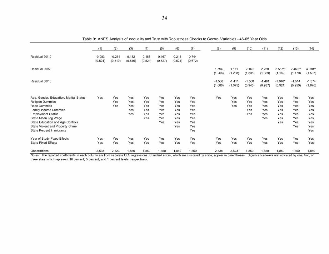
Table 8 presents estimates for the model above using a sample of 20-45 year olds in the ANES, which accounts for the bulk of the decline in trust in the United States. The estimate of inequality on trust is presented after adding more controls in stepwise fashion. The first column’s specification includes only basic controls for age, education, marital status, gender, and fixed-effects for each state and survey year. The estimated effect of the residual P90/P10 ratio on trust with this specification is negative, but not significant. Adding further controls for religion and race to the specification increases the size of the coefficient and renders it significant at the 10 percent level. Adding individual characteristics, such as family income and employment status, yields more significant results, as does the addition of state-level controls for the average wage, crime rate, percent immigrants, and the age and education composition. The full specification in column (7) yields a negative and significant relationship between the residual P90/P10 ratio and a person’s level of “trust in people.” However, given that the coefficient increases in size and significance with the addition of more controls, this result is somewhat sensitive to the choice of specification. The panel on the right side of Table 8 breaks down the residual P90/P10 ratio into two components: inequality at the top of the distribution (residual P90/P50 ratio) versus inequality at the bottom (residual P50/P10 ratio). The results show that the two components have very different effects on trust. In particular, inequality at the top has no effect on trust, while increasing inequality at the bottom of the income distribution lowers trust significantly. Both findings are robust to the inclusion or exclusion to a broad range of control variables. Although this robustness does not prove that the results would be insensitive to the inclusion of factors omitted even in the full specification, the lack of sensitivity to the various individual and state-level controls supports the identifying assumption that the findings on the right-side of Table 8 are not due to omitted variable bias. Table 9 repeats the analysis in Table 8 using an older sample composed of 46-65 year olds. The results differ from Table 8 in that the residual P90/P10 ratio is insignificant for all specifications. The residual P50/P10 ratio is also insignificant in most of the specifications, but is consistently negative with t-statistics above 1.3. Similar to Table 8, inequality at the top of the distribution (residual P90/P50 ratio) has a very different effect relative to inequality at the bottom. The residual P90/P50 ratio is always positive and even significant in the last three specifications. Looking at Table 8 and Table 9 together, it appears that “trust in people” in the United States reacts differently to alternative sources of inequality: inequality at the bottom reduces trust, while inequality at the top does not – and may even increase trust for older individuals. The results are stronger for individuals in their prime working years relative to those above the age of 45, which may be due to the idea that older workers formulated their views about trust in response to the level of inequality when they were younger, rather than reacting to current levels during the latter part of their working career. Given that the response to inequality

17

appears to be stronger for the younger sample, the rest of the analysis will focus on understanding this phenomenon further for that sample. Table 10 examines the relationship between various measures of inequality with several viewpoints and social capital variables in the ANES. Each coefficient represents a separate regression using the full set of controls (column (7) in Tables 8 and 9). The residual P90/P10 ratio is significant and negative for trust in people, people are fair, people are helpful, the trust in government index, and a willingness to spend more on the poor. Using the P90/P10 ratio of actual wages, as opposed to residual wages, yields similar results, although somewhat weaker. Using the Gini coefficient, taken from the Bureau of the Census, yields similar patterns for the social capital variables related to trust in people and government. Furthermore, inequality at the top (residual P90/P50 ratio) and at the bottom (residual P50/P10 ratio) are found to reduce trust in people and government, with some evidence that they reduce a person’s willingness to spend more money on the poor. In contrast, none of the various measures of inequality have an effect on a person’s view about whether they think it is a problem that chances are unequal, or cause individuals to favor a larger role for government. The one measure of inequality in Table 10 that has no effect on any measure of social capital is the return to education. Despite the increase in the return to education over recent decades, this variable has no effect on trust in people, trust in government, or views about spending on the poor. This finding helps to understand why the results for residual inequality are stronger than overall inequality, since the overall inequality measure includes the insignificant effect of the return to education. Furthermore, the stark contrast in the findings using this measure versus residual inequality once again suggests that inequality from different sources has potentially different effects on the social capital outcomes of individuals. Inequality between education groups does not affect trust, but inequality within groups (residual inequality represents inequality within education, age, industry, and occupation) reduces trust in people and government. That is, when people see larger income gaps among people who are similar to them in terms of age, education, and type of work, this seems to reduce trust. But, when they see gaps increasing between people who have made different educational and career choices, this has no effect on trust. One interpretation of this pattern is that people have a better understanding, and sense of fairness, of inequality that stems from differences in human capital decisions and investments. However, when they see larger gaps due to luck or unexplained factors, this reduces their trust in others and government. Of course, residual inequality is composed of many factors that are not associated with random luck, such as effort and unobserved ability, but random factors are more likely to be affecting residual inequality relative to the return people get on their education investments and career decisions regarding their occupation and industry.

18

Tables 11 and 12 examine additional sources of inequality at the bottom and the top of the distribution, respectively. Table 11 shows that the results for the overall P50/P10 ratio are similar to those using the residual P50/P10, but there is no evidence that the employment rate of non-college individuals, which can be considered an outcome of wage inequality, has an effect on trust. The poverty rate, taken directly from the U.S. Census Bureau for each state, does not have a robust impact on trust in people or government either. 9 In Table 12, the residual P90/P50 ratio has a more significant effect than the total P90/P50 ratio, most likely because the latter includes the return to education which was seen to have no effect in Table 10. Table 12 also examines the share of income going to the top 1%, top 5%, and top 10% of the income distribution. These variables are taken from the World Top Incomes Database put together by Mark Frank, Estelle Sommeiller, Mark Price, and Emmanuel Saez. The results for these “top shares” indicate a weak negative effect, although largely insignificant, on trust in people and government. Increases in the top shares do seem to reduce a person’s willingness to spend more on the poor. But, overall, the top shares do not have a robust impact on the various measures of social capital. Tables 11 and 12 showed significant negative effects of the main measures of inequality at the top and bottom of the distribution. In order to see which effect is more dominant, Table 13 presents an analysis using the four main, but distinct, measures of inequality in one specification. These measures are distinct because residual inequality is by construction orthogonal to the return to education, and the top 5% share represents inequality at the top that lies even above the residual P90/P50 ratio. In addition, the inclusion of multiple measures of inequality implies that we are controlling for the myriad of unobserved drivers of income inequality, while isolating the individual effect of each one. The results in Table 13 clearly indicate that the residual P50/P10 is the dominant factor on trust in people and government, with the other measures insignificant. This finding emphasizes that inequality at the bottom of the distribution is the main type of inequality that affects trust in the United States. Tables 14 examines whether the effect of inequality at the bottom differs by gender and between education and income groups. The results are similar for men and women, but much stronger for non-college graduates relative to college graduates. In addition, the findings for the lowest income group appear to be larger than the middle and top groups – although the finding that inequality reduces a person’s willingness to spend more money on

9 The measurement of poverty in the United States differs from measures of wage inequality in the bottom of the distribution in a number of important respects. First, poverty is a household concept and includes all sources of income whereas wage inequality measures are based on individual labour earnings. Second, in contrast to the measurement of poverty in European countries, poverty in the United States is based on an absolute poverty line and hence is not purely a relative concept. Differences in poverty across US states reflect both differences in the average level of income and differences in its distribution.

19

the poor is confined to the middle and upper income categories. Overall, Table 14 suggests that income inequality at the bottom of the distribution reduces trust mainly for those adversely affected by the increase in that type of inequality. Table 15 examines whether the effect of inequality at the top differs by the same groups. The results are rather similar across gender and education groups, but the upper income group is clearly more negatively affected by increasing inequality at the top of the distribution. Interestingly, it is the group that benefits from inequality at the top that seems to be responding by lowering their trust – perhaps an indication that their increasing separation according to their income translates into greater isolation, in their values and perhaps in terms of their places of work and residential neighborhoods, from lower income groups. It is worth noting that the estimated effect of inequality on trust using the ANES data is significant not only in the statistical sense, but also in magnitude. The coefficient on the residual P90/P10 ratio in Table 8 with the full specification is -0.909, and multiplying that with the actual increase in the residual P90/P10 ratio from 1980 to 2000 (Figure 2) of 0.067 yields a predicted decline in trust of 0.06. Table 3 indicates that the unexplained decline in trust is approximately 0.14 (the trend coefficient of -0.007 multiplied by 20 years). Thus, the increase inequality explains just about 44 percent of the unexplained decline in trust levels in the United States during this time period.

V. ANALYSIS FOR EUROPEAN COUNTRIES

We now turn to the European Social Survey (ESS) to perform a similar analysis which exploits variation across 25 countries and over time (2002-2014). Table 16 presents estimates of the effect of various sources of household income inequality on trust in other people, and shows how the results are affected by the addition of more control variables to the specification. In addition, the results are presented for the younger (ages 25-45) and the older samples (ages 46-65). The estimated effect of the P90/P10 income ratio is negative and significant for the specification with all of the available controls (age, gender, education, marital status, employment status, percent immigrants, and GDP per capita), but is not significant for specifications that do not include the latter two. The gini coefficient is significant and robust to the choice of specification, as are the P50/P10 ratio and the poverty rate (defined as the share of households with incomes of less than half the median). Inequality at the top of the distribution, represented by the P90/P50 ratio or the top 5% share, is not significant across specifications. The overall findings in Table 16 point to a significant and negative effect of inequality on trust, but mostly confined to inequality stemming from the lower part of the income distribution – as represented by the P50/P10 ratio and the poverty rate. These findings are similar to those presented for the United States using the ANES data. Although the poverty

20

rate was not significant for the United States, the poverty rate in Europe is defined in relative terms, relative to half the median, rather than in absolute terms with respect to the national poverty line as is done in the United States. Since the results in Table 16 are very similar for the two age groups, unlike the analysis of the United States, the remaining tables merge the two samples together. Table 17 presents the estimates for various measures of inequality on several social capital views. The gini coefficient is significant for all the outcomes of interest – lowering trust and how much they believe others are fair and helpful. In addition, a larger gini coefficient increases one’s belief that the government should reduce income gaps, while lowering satisfaction in government, satisfaction in life, and personal happiness. Similar effects on trust, fairness, and helpfulness are found with other measures of inequality, such as the P90/P10 ratio, the P50/P10 ratio, the poverty rate, and the poverty gap. The latter two also have similar impacts on one’s view that government should reduce income gaps, and satisfaction in life and in government. These findings stand in stark contrast to those found for the top income shares – the top 1%, top 5%, and the top 10%. Increases in these shares seem to increase the view that the government should reduce income gaps, and there is some evidence of a reduction in life satisfaction, but no evidence that they lower trust in other people. In fact, the estimated coefficients on trust, fairness, and helpfulness are all positive, and some of them are significant. Table 17 reveals that employment rates in Europe have little effect on the various trust measures, but lower employment rates do seem to lower satisfaction in government and life. Table 18 presents the results after including various components of inequality in one specification. In contrast to the analysis for the United States where the P50/P10 ratio dominated the other types of inequality, the results for the ESS are rather mixed. The P90/P50 and the P50/P10 ratios have similar effects when included in the same specification, and the employment rate is significant for several outcomes as well. Overall, it appears that inequality from all over the spectrum has a more significant, negative impact on trust and satisfaction in government than in the United States. Table 19 examines whether the effect of the P90/P10 ratio on various social capital outcomes are different across gender and education groups. Both in terms of size and significance, the results are very similar for college graduates and non-college graduates, and for men and women as well. Table 20 reveals a similar pattern for the effect of inequality at the bottom of the distribution using the P50/P10 ratio, and Table 21 displays similar findings for inequality at the top using the P90/P50 ratio. The one exception is the significant and positive effect of the P90/P50 ratio on satisfaction in government for college graduates, while coming out insignificant for non-college graduates.

21

Overall, inequality seems to reduce an individual’s sense of trust, fairness, and helpfulness in others, and this finding is rather consistent across gender and education groups. This stands in contrast to the finding for the United States where inequality, mostly at the bottom of the distribution, reduces trust but mainly for those that are adversely affected by that type of inequality. In Europe, the effect is a more general reaction, rather than a seemingly more personal one in the United States. Consistent with this idea, there is some evidence that inequality in Europe (the gini, the top shares, the poverty rate, and the poverty gap) is leading individuals to believe that the government should reduce income gaps, but this finding is not confined to those that are directly benefiting or being hurt by increases in inequality.

VI. CONCLUSION

This paper analyzed the effect of inequality on an individual’s level of trust in others, as well as various other measures of social capital. The analysis was conducted for the United States using the ANES and exploiting variation in inequality across states and years, and for Europe using the ESS and variation across countries and time. The results suggest that inequality at the bottom of the distribution lowers an individual’s sense of trust in others – in the United States and in Europe. A causal interpretation of this finding is bolstered by the robustness of the effect to the inclusion and exclusion of several control variables – which supports the identifying assumption that the results would not be sensitive to omitted factors from the full-specification. In addition, these findings are robust to the inclusion of various other measures of inequality in the same specification – which controls for a myriad of other unobserved factors which may be driving the increasing inequality trends in many developed countries over recent decades. For the United States, it appears that inequality at the bottom of the distribution is the main component of inequality that reduces trust, and this phenomenon is mainly confined to those that are negatively impacted by that component of inequality – individuals who are less educated and those at the lower third of the income distribution. The trust levels of Europeans are also negatively affected by increasing inequality levels. However, in contrast to the United States, the impact of inequality on trust in Europe is more general. Inequality at the top and bottom of the distribution seem to have a negative impact, and the negative effect is shared across education groups. There is also some evidence that inequality from all over the spectrum is causing Europeans to desire more government action to reduce income gaps. In the United States, there is little evidence that this is case. For both the United States and Europe, the results do not provide any support for the idea that increases in inequality at the very top of the distribution, such as the top 1 percent or top 5 percent shares, have led to a decline in overall trust levels. The significant negative effect of inequality on trust is apparently not driven by inequalities at these extreme ends of the

22

distribution. This finding may be due to the idea that very few people are directly affected by those forms of inequality. Overall, our results suggest that the increasing income inequality trends in recent decades for many advanced countries may have negatively affected overall trust levels, and thereby, increased social gaps in society in the wake of widening income gaps. Given that trust has been found to be an important determinant of the macro-economic performance of the many countries, these findings suggest an important, albeit indirect, way that increasing inequality may be adversely affecting a country’s growth and development over time.

23

References

Alesina A. and E. La Ferrara (2002), “Who Trusts Others?”, Journal of Public Economics,

85, 207–234. Alesina, A., and P. Giuliano (2016), “Culture and Institutions”, Journal of Economic

Literature, forthcoming. Alesina, A., G. Cozzi, and N. Mantovan (2012), “The Evolution of Ideology, Fairness and

Redistribution”, Economic Journal, 122: 1244–1261. Algan, Y. and P. Cahuc (2010), “Inherited Trust and Growth”, American Economic Review,

Vol. 100, December 2010: 2060–2092. Algan, Y. and P. Cahuc (2013), “Trust, Growth, and Well-Being: New Evidence and Policy

Implications,” in Handbook of Economic Growth, P. Aghion and S. Durlauf (eds.), North-Holland, Elsevier.

Barone, G., and S. Mocetti (2016), “Inequality and Trust: New Evidence from Panel Data”,

Economic Inquiry, 54 (2), April 2016. Bloom, N., R. Sadun, and J. Van Reenen (2012), “The Organization of Firms across

Countries”, Quarterly Journal of Economics, 127 (4): 1663-1705. Cingano, F. (2014), “Trends in Income Inequality and its Impact on Economic Growth”,

OECD Social, Employment and Migration Working Paper, No. 163. Cingano, F. and P. Pinotti (2016), “Trust, Firm Organization and the Structure of

Production”, Journal of International Economics, Vol 100, pp. 1-13. Coleman, J.S. (1990), Foundations of Social Theory, Harvard University Press, Cambridge,

Mass. Dabla-Norris, E., K. Kochhar, N. Suphaphiphat, F. Ricka, E. Tsounta (2015), “Causes and

Consequences of Income Inequality : A Global Perspective”, Staff Discussion Notes, No. 15/13.

Galor, O. and J. Zeira (1993). “Income Distribution and Macroeconomics,” Review of

Economic Studies, 60(1), 35-52. Guiso, L., Sapienza, P., and L. Zingales (2004), “The Role of Social Capital in Financial

Development”, American Economic Review, 94(3), 526–556. Guiso, L., Sapienza, P., and L. Zingales (2006), “Does Culture Affect Economic

Outcomes?”, Journal of Economic Perspectives, 20(2): 23–48.

24

Guiso, L., Sapienza, P., and L. Zingales (2008), “Trusting the Stock Market,” Journal of Finance, 63(6), 2557–2600.

Guiso, L., Sapienza, P. and L. Zingales (2009), “Cultural Biases in Economic Exchange?”,

Quarterly Journal of Economics, 124(3), 1095–1131. Gustavsson, M. and H. Jordahl (2008), “Inequality and trust in Sweden: Some inequalities

are more harmful than others”, Journal of Public Economics, vol. 92(1-2), pages 348-365, February.

Jordahl, H. (2007), “Inequality and Trust”, Working Paper Series 715, Research Institute of

Industrial Economics. Knack, S. and P. Keefer (1997), “Does Social Capital Have an Economic Payoff? A Cross-

Country Investigation”, Quarterly Journal of Economics, 112(4), 1252–1288. La Porta R., Lopez-de-Silanes, F., Shleifer, A., and R. Vishny (1999), “The Quality of

Government”, Journal of Law Economics and Organization, 15(1), 222–279. Nannicini, T., Stella, A., Tabellini, G., and U. Troiano (2012), “Social Capital and Political

Accountability”, American Economic Journal: Economic Policy, 5, 222–250. Ostry, J. D., A. Berg, and C. Tsangarides (2014), “Redistribution, Inequality, and Growth.”

IMF Staff Discussion Note 14/02. Putnam, R. D. (1995), “Tuning In, Tuning Out: The Strange Disappearance of Social Capital

in Americaǁ”, Political Science and Politics, v. 28 (4), 664-665. Putnam, R.D. (2001), Our Kids: The American Dream in Crisis, Simon & Schuster. Rothstein, B. and E.M. Uslaner (2005), “All for All: Equality, Corruption, and Social Trust”,

World Politics, Vol.58, pp. 41-72. Ruggles, Steven, Matthew Sobek, Trent Alexander, Catherine A. Fitch, Ronald Goeken,

Patricia Kelly Hall, Miriam King, and Chad Ronnander. 2010. Integrated Public Use Microdata Series: Version 3.0 [Machine-readable database]. Minneapolis, MN: Minnesota Population Center [producer and distributor].

Sarracino, Francesco and Mikucka, Malgorzata (2016). “Social Capital in Europe from 1990

to 2012: Trends and Convergence,” Social Indicators Research, February, 1-26. Tabellini, G. (2008), “Institutions and Culture”, Journal of the European Economic

Association, 6(2–3), 255–294. Tabellini, G. (2010), “Culture and Institutions: Economic Development in the Regions of

Europe”, Journal of the European Economic Association, 8(4), 677–716. Tesei, A. (2015), “Trust and Racial Income Inequality: Evidence from the U.S”, Working

Papers 737, Queen Mary University of London, School of Economics and Finance.

25

Twenge, J. M., W.K. Campbell and N. T. Carter (2014), “Declines in Trust in Others and

Confidence in Institutions Among American Adults and Late Adolescents, 1972–2012”, Psychological Science, September 9, 2014, 1-12.

Zak, P.J. and S. Knack, (2001), “Trust and growth”, Economic Journal, 111 (470), 291–321.

26

Census Year

Year of ANES Study 1976 1978 1980 1982 1988 1990 1992 1998 2000 2002 2008 2012

Age 39.85 39.29 39.872 40.32 39.72 39.77 39.57 40.70 40.83 40.07 41.92 42.76Male 0.430 0.459 0.440 0.458 0.436 0.481 0.492 0.470 0.455 0.455 0.450 0.480HS Dropout 0.255 0.224 0.214 0.175 0.167 0.180 0.142 0.115 0.109 0.108 0.091 0.090HS Graduate 0.373 0.396 0.385 0.346 0.367 0.372 0.348 0.334 0.326 0.336 0.302 0.346Some College 0.201 0.204 0.219 0.270 0.247 0.225 0.251 0.297 0.302 0.299 0.306 0.254College Grad 0.127 0.122 0.118 0.127 0.156 0.151 0.178 0.154 0.178 0.178 0.204 0.206Advanced Degree 0.044 0.053 0.063 0.081 0.064 0.072 0.080 0.100 0.085 0.079 0.097 0.105Married 0.683 0.699 0.676 0.635 0.602 0.621 0.617 0.642 0.631 0.632 0.529 0.648Protestant 0.636 0.617 0.614 0.635 0.641 0.573 0.586 0.487 0.537 0.554 0.568 0.308Catholic 0.252 0.247 0.241 0.224 0.235 0.251 0.235 0.334 0.261 0.265 0.178 0.206Jewish 0.026 0.026 0.026 0.017 0.015 0.018 0.015 0.019 0.017 0.013 0.015 0.017White 0.864 0.845 0.825 0.846 0.745 0.746 0.749 0.727 0.725 0.735 0.719 0.699Black 0.102 0.108 0.117 0.113 0.134 0.128 0.129 0.115 0.118 0.110 0.123 0.125Income - Bottom Third 0.253 0.292 0.262 0.287 0.274 0.277 0.286 0.270 0.337 . 0.276 0.303Income - Middle Third 0.335 0.331 0.396 0.303 0.371 0.323 0.314 0.346 0.312 . 0.403 0.364Income - Top Third 0.412 0.377 0.342 0.410 0.355 0.400 0.399 0.384 0.351 . 0.322 0.334Not Employed 0.097 0.075 0.097 0.104 0.088 0.100 0.115 0.090 0.100 0.077 0.131 0.149

Minimum Observations 1681 1684 1165 1031 1542 1444 1872 980 1275 1206 1747 4516

Table 1: ANES Summary Statistics - Means of Demographic Variables

1980 1990 2000 2010

27

Census Year

Year of ANES Study 1976 1978 1980 1982 1988 1990 1992 1998 2000 2002 2008 2012

Trust People 0.541 0.451 0.405 0.498 0.504People are Fair 0.629 . 0.552 0.670 0.687People are Helpful 0.553 0.589 0.620 0.676Trust Index -0.016 -0.005 -0.047 -0.064 -0.132

Trust Govt to Benefit All 0.232 0.247 0.207 0.286 0.315 0.247 0.222 0.317 0.356 0.512 0.301 0.194Trust Govt to Do Right 0.342 0.299 0.236 0.327 0.416 0.279 0.289 0.400 0.423 0.544 0.302 0.230Trust Govt Index 29.708 29.425 26.053 30.894 34.416 28.948 28.936 33.896 36.481 43.208 25.882 22.120

Never Attend Religious Service 0.209 0.236 0.243 0.220 0.209 0.334 0.342 0.333 0.336 0.346 0.399 0.449Increase Spending on Poor 1.479 1.436 1.497 1.543 1.163It is a problem if chances are unequal 3.279 3.355 3.446 3.459 3.463 3.390Favor Larger Government 0.702 0.656 0.601 0.608 0.475

Minimum Observations 1402 1879 1135 1127 1415 1540 1754 1007 715 534 827 2396Maximum Observations 1775 1913 1294 1144 1640 1562 2002 1028 1479 1214 1845 4666

1980 1990 2000 2010

Table 2: ANES Summary Statistics - Means of Trust and Other Social Capital Variables

28

Ages 20 - 45 Ages 46-65-1 (2) (3) (4) (5) (6) (7) (8) (9) (10) (11) (12) (13) (14) (15) (16) (17) (18)

Year -0.004*** -0.005*** -0.005*** -0.005*** -0.006*** -0.006*** -0.005*** -0.007*** -0.007*** -0.000 -0.000 -0.000 -0.000 -0.004*** -0.005*** -0.003*** -0.004*** -0.004***-0.001 (0.001) (0.001) (0.001) (0.001) (0.001) (0.001) (0.001) (0.001) (0.001) (0.001) (0.001) (0.001) (0.001) (0.001) (0.001) (0.001) (0.001)

Age 0.138* 0.138* 0.136* 0.067 0.050 0.057 0.037 0.023 0.238 0.238 0.162 -0.235 -0.268 -0.543 -0.389 -0.149(0.080) (0.080) (0.080) (0.078) (0.077) (0.075) -0.081 (0.081) (0.454) (0.454) (0.429) (0.372) (0.377) (0.390) (0.465) (0.457)

Age Squared -0.004 -0.004 -0.004 -0.002 -0.001 -0.002 -0.001 -0.000 -0.004 -0.004 -0.003 0.005 0.005 0.010 0.007 0.003(0.003) (0.003) (0.003) (0.002) (0.002) (0.002) (0.003) (0.003) (0.008) (0.008) (0.008) (0.007) (0.007) (0.007) (0.008) (0.008)

Age Cubed 0.000 0.000 0.000 0.000 0.000 0.000 0.000 0.000 0.000 0.000 0.000 -0.000 -0.000 -0.000 -0.000 -0.000(0.000) (0.000) (0.000) (0.000) (0.000) (0.000) (0.000) (0.000) (0.000) (0.000) (0.000) (0.000) (0.000) (0.000) (0.000) (0.000)

Male Dummy 0.058*** 0.041** 0.065*** 0.045* 0.040 0.038 0.064*** 0.036* 0.059 0.044 0.066 0.067(0.018) (0.016) (0.023) (0.025) (0.030) (0.029) (0.019) (0.021) (0.043) (0.041) (0.042) (0.041)

HS Graduate 0.181*** 0.177*** 0.162*** 0.162*** 0.157*** 0.185*** 0.177*** 0.130*** 0.095** 0.085**(0.031) (0.031) (0.030) (0.029) (0.027) (0.039) (0.039) (0.035) (0.040) (0.041)

Some College 0.259*** 0.257*** 0.237*** 0.234*** 0.231*** 0.303*** 0.301*** 0.260*** 0.228*** 0.207***(0.028) (0.028) (0.027) (0.031) (0.032) (0.032) (0.032) (0.028) (0.039) (0.041)

College Grad 0.429*** 0.425*** 0.392*** 0.370*** 0.366*** 0.448*** 0.438*** 0.384*** 0.308*** 0.288***(0.034) (0.033) (0.033) (0.041) (0.041) (0.040) (0.041) (0.034) (0.045) (0.048)

Advanced Degree 0.447*** 0.442*** 0.405*** 0.388*** 0.381*** 0.458*** 0.453*** 0.410*** 0.347*** 0.338***(0.039) (0.039) (0.039) (0.055) (0.056) (0.035) (0.035) (0.031) (0.048) (0.051)

Married 0.072*** 0.036 0.015 0.013 0.092*** 0.046 -0.010 0.005(0.021) (0.022) (0.025) (0.025) (0.030) (0.031) (0.034) (0.036)

Married*Male -0.035 -0.014 -0.027 -0.023 -0.044 -0.019 -0.036 -0.040(0.034) (0.035) (0.040) (0.038) (0.047) (0.044) (0.050) (0.050)

Religion Dummies Yes Yes Yes Yes Yes YesRace Dummies Yes Yes Yes Yes Yes YesFamily Income Dummies Yes Yes Yes YesEmployment Status Yes Yes Yes YesState Fixed-Effects Yes Yes

Observations 4,165 4,165 4,165 4,165 4,135 4,135 4,113 3,337 3,337 2,600 2,600 2,600 2,600 2,576 2,576 2,561 1,883 1,883

Table 3: ANES Trends in "Trust People" in the United States from 1980-2000

29

Trust People

People are Fair

People are Helpful

Trust Index

Trust Government

Index

Never Attend Religious Service

Increase Spending on

Poor

It is a problem if chances are

unequal

Favor Larger Government

(1) (2) (3) (4) (5) (6) (7) (8) (9)

Year -0.007*** -0.001 0.000 -0.007*** -0.124*** 0.001** -0.016*** -0.006*** -0.010***(0.001) (0.001) (0.001) (0.002) (0.025) (0.000) (0.002) (0.002) (0.001)

Observations 3,337 2,125 2,658 3,220 10,986 11,465 5,096 6,088 5,080

Table 4: ANES Trends in Trust and Other Social Capital Variables

Notes: The reported coefficients are from separate OLS regressions. Standard errors, which are clustered by state, appear in parentheses. Significance levels are indicated by one, two, or three stars which represent 10 percent, 5 percent, and 1 percent levels, respectively. Each regression includes personal controls (age, education, gender, marital status, race category, religion group, income category, and employment status) and fixed-effects for each state.

30

Mean Count Mean Count Mean Count Mean Count Mean Count Mean Count Mean Count

Age 41.946 27907 42.063 31616 42.526 28307 42.284 37559 42.931 33652 43.020 35491 43.356 24805Male 0.480 27897 0.467 31588 0.466 28286 0.463 37550 0.461 33642 0.464 35478 0.473 24799College Graduate 0.248 27758 0.258 31385 0.314 28215 0.310 37493 0.324 33536 0.343 35313 0.349 24708Married 0.681 27667 0.666 31451 0.663 28025 0.657 37306 0.635 33580 0.641 35361 0.647 24715Working Last 7 Days 0.648 27540 0.632 31481 0.676 28172 0.646 37404 0.626 33563 0.640 35261 0.693 24724GDP Per Capita 10.408 27907 10.360 30405 10.462 23816 10.394 28457 10.402 26266 10.422 26752 10.475 23369

Trust People 5.064 27839 4.937 31521 5.027 28180 4.681 37454 4.865 33563 4.914 35378 5.242 24773People are Fair 5.592 27750 5.479 31395 5.590 27990 5.229 37237 5.366 33402 5.438 35177 5.770 24694People are Helpful 4.730 27809 4.674 31469 4.761 28159 4.484 37390 4.646 33489 4.783 35335Strongly Agree Govt Should Reduce Gaps 0.250 27882 0.283 31585 0.300 28268 0.303 37528 0.352 33627 0.354 35434 0.319 24786Satisfied with Govt 4.230 25817 4.243 30614 4.290 27472 3.785 36766 3.666 32984 3.816 34794 4.028 24338Satisfied with Life 7.029 27783 6.844 31499 6.775 28180 6.544 37282 6.609 33523 6.694 35309Happiness 7.406 27800 7.238 31471 7.188 28118 6.986 37260 7.019 33394 7.104 35246 7.397 24723More Religious 4.706 27734 4.592 31402 4.469 28073 4.645 37134 4.415 33289 4.494 35111 3.997 24632

Table 5: Summary Statistics of Demographics and Social Capital Variables in the ESS Sample

2002 2004 2006 2008 2010 2012 2014

31

Mean Count Mean Count Mean Count Mean Count Mean Count Mean Count Mean Count

Disposable Income 90/10 3.071 19188 3.249 23746 3.318 21821 3.309 23552 3.396 27258 3.171 21431 3.354 4882Gini - Disposable Income 0.258 1405 0.306 14679 0.305 10747 0.298 13894 0.301 17978 0.294 26752 0.288 1174Disposable Income 90/50 1.851 19188 1.927 23746 1.950 21821 1.979 23552 1.981 27258 1.919 21431 1.920 4882Top 1% Income Share 8.830 16957 9.348 15868 9.637 14211 9.084 12814 8.509 8776 8.770 6002Top 5% Income Share 21.374 15504 21.985 14275 22.082 13141 21.507 11782 21.009 8776 21.648 6002Top 10% Income Share 32.155 16957 33.017 15868 33.100 14211 32.355 12814 31.625 8776 32.588 6002Disposable Income 50/10 1.638 19188 1.676 23746 1.689 21821 1.661 23552 1.706 27258 1.648 21431 1.750 4882Poverty Rate 0.062 1405 0.103 14679 0.101 10747 0.097 13894 0.100 17978 0.097 26752 0.101 1174Poverty Gap 0.248 1405 0.302 17373 0.298 16018 0.303 19587 0.320 24320 0.315 17056Employment Rate 77.999 22967 79.016 25825 80.734 23816 79.489 28457 78.634 26266 78.928 27734 80.237 23369Employment Rate - Ages 25-39 0.780 27907 0.757 31616 0.800 28307 0.766 37559 0.755 33652 0.741 35491 0.797 24805Unemployment Rate - Ages 25-39 0.076 27907 0.098 31616 0.072 28307 0.103 37559 0.132 33652 0.140 35491 0.097 24805

2014

Table 6: Summary Statistics of Inequality Measures in the ESS Sample

2002 2004 2006 2008 2010 2012

32

(1) (2) (3) (4) (5) (6) (7)

Year 0.028*** 0.028*** 0.028*** 0.009*** 0.010*** -0.009*** 0.002(0.002) (0.002) (0.002) (0.002) (0.002) (0.002) (0.003)

Age -0.043* -0.043* -0.172*** -0.174*** -0.188*** -0.198***(0.026) (0.026) (0.025) (0.026) (0.025) (0.024)

Age Squared 0.001** 0.001** 0.004*** 0.004*** 0.005*** 0.005***(0.001) (0.001) (0.001) (0.001) (0.001) (0.001)

Age Cubed -0.000*** -0.000*** -0.000*** -0.000*** -0.000*** -0.000***(0.000) (0.000) (0.000) (0.000) (0.000) (0.000)

Male 0.087*** 0.087*** 0.058*** 0.159*** 0.122*** 0.111***(0.017) (0.017) (0.016) (0.029) (0.029) (0.028)

Educ ISCED 2 0.641*** 0.638*** 0.313*** 0.110***(0.037) (0.037) (0.036) (0.037)

Educ ISCED 3 0.816*** 0.813*** 0.509*** 0.443***(0.033) (0.033) (0.031) (0.035)

Educ ISCED 4 1.306*** 1.302*** 0.894*** 0.739***(0.046) (0.046) (0.045) (0.047)

Educ ISCED 5 1.753*** 1.754*** 1.294*** 1.179***(0.033) (0.034) (0.033) (0.035)

Married -0.055** 0.014 0.027(0.027) (0.026) (0.026)

Married*Female 0.148*** 0.098*** 0.095***(0.035) (0.035) (0.034)

GDP Per Capita 1.899*** 0.374**(0.028) (0.149)

Country Fixed-Effects Yes

Observations 186,552 186,467 186,467 185,615 184,613 184,613 184,613

Table 7: ESS Trends in "Trust People" in Europe from 2002-2014

33

(1) (2) (3) (4) (5) (6) (7) (8) (9) (10) (11) (12) (13) (14)

Residual 90/10 -0.529 -0.630* -0.765* -0.793* -0.764* -0.685* -0.909**(0.369) (0.368) (0.431) (0.422) (0.420) (0.401) (0.415)

Residual 90/50 0.196 -0.115 0.491 0.485 0.303 0.138 -0.249(1.032) (1.134) (1.055) (1.104) (1.074) (0.948) (1.000)

Residual 50/10 -1.083* -1.024 -1.735** -1.735** -1.513** -1.281* -1.308*(0.616) (0.673) (0.720) (0.722) (0.705) (0.677) (0.696)

Age, Gender, Education, Marital Status Yes Yes Yes Yes Yes Yes Yes Yes Yes Yes Yes Yes Yes YesReligion Dummies Yes Yes Yes Yes Yes Yes Yes Yes Yes Yes Yes YesRace Dummies Yes Yes Yes Yes Yes Yes Yes Yes Yes Yes Yes YesFamily Income Dummies Yes Yes Yes Yes Yes Yes Yes Yes Yes YesEmployment Status Yes Yes Yes Yes Yes Yes Yes Yes Yes YesState Mean Log Wage Yes Yes Yes Yes Yes Yes Yes YesState Education and Age Controls Yes Yes Yes Yes Yes YesState Violent and Property Crime Yes Yes Yes YesState Percent Immigrants Yes Yes

Year of Study Fixed-Effects Yes Yes Yes Yes Yes Yes Yes Yes Yes Yes Yes Yes Yes YesState Fixed-Effects Yes Yes Yes Yes Yes Yes Yes Yes Yes Yes Yes Yes Yes Yes

Observations 4,076 4,054 3,283 3,283 3,283 3,283 3,283 4,076 4,054 3,283 3,283 3,283 3,283 3,283

Table 8: ANES Analysis of Inequality and Trust with Robustness Checks to Control Variables - 20-45 Year Olds

Notes: The reported coefficients in each column are from separate OLS regressions. Standard errors, which are clustered by state, appear in parentheses. Significance levels are indicated by one, two, or three stars which represent 10 percent, 5 percent, and 1 percent levels, respectively.

34

(1) (2) (3) (4) (5) (6) (7) (8) (9) (10) (11) (12) (13) (14)

Residual 90/10 -0.083 -0.251 0.182 0.186 0.167 0.215 0.744(0.524) (0.510) (0.516) (0.524) (0.527) (0.521) (0.672)

Residual 90/50 1.594 1.111 2.169 2.258 2.567** 2.459** 4.018**(1.266) (1.288) (1.335) (1.369) (1.169) (1.170) (1.507)

Residual 50/10 -1.508 -1.411 -1.500 -1.481 -1.648* -1.514 -1.374(1.080) (1.075) (0.945) (0.937) (0.924) (0.950) (1.070)

Age, Gender, Education, Marital Status Yes Yes Yes Yes Yes Yes Yes Yes Yes Yes Yes Yes Yes YesReligion Dummies Yes Yes Yes Yes Yes Yes Yes Yes Yes Yes Yes YesRace Dummies Yes Yes Yes Yes Yes Yes Yes Yes Yes Yes Yes YesFamily Income Dummies Yes Yes Yes Yes Yes Yes Yes Yes Yes YesEmployment Status Yes Yes Yes Yes Yes Yes Yes Yes Yes YesState Mean Log Wage Yes Yes Yes Yes Yes Yes Yes YesState Education and Age Controls Yes Yes Yes Yes Yes YesState Violent and Property Crime Yes Yes Yes YesState Percent Immigrants Yes Yes

Year of Study Fixed-Effects Yes Yes Yes Yes Yes Yes Yes Yes Yes Yes Yes Yes Yes YesState Fixed-Effects Yes Yes Yes Yes Yes Yes Yes Yes Yes Yes Yes Yes Yes Yes

Observations 2,538 2,523 1,850 1,850 1,850 1,850 1,850 2,538 2,523 1,850 1,850 1,850 1,850 1,850

Table 9: ANES Analysis of Inequality and Trust with Robustness Checks to Control Variables - 46-65 Year Olds

Notes: The reported coefficients in each column are from separate OLS regressions. Standard errors, which are clustered by state, appear in parentheses. Significance levels are indicated by one, two, or three stars which represent 10 percent, 5 percent, and 1 percent levels, respectively.

35

Trust People

People are Fair

People are Helpful

Trust Index

Trust Government

Index

Never Attend Religious Service

Increase Spending on

Poor

It is a problem if chances are

unequal

Favor Larger Government

(1) (2) (3) (4) (5) (6) (7) (8) (9)

Residual 90/10 -0.909** -2.042*** -2.118*** -3.620*** -38.931** 0.516 -2.539*** 1.067 -0.442(0.415) (0.458) (0.510) (0.803) (17.102) (0.335) (0.582) (0.904) (0.391)3,283 2,071 2,607 3,167 10,910 11,407 5,087 6,081 5,073

Total 90/10 -0.337 -1.464*** -1.141** -1.909*** -24.557** 0.267 -0.873 0.367 -0.328(0.309) (0.394) (0.451) (0.574) (9.310) (0.168) (0.553) (0.698) (0.290)3,283 2,071 2,607 3,167 10,910 11,407 5,087 6,081 5,073

Gini -3.579** -6.597*** -6.682*** -13.376*** -118.231** 0.971 2.480 0.682 -0.759(1.558) (2.112) (2.273) (3.247) (56.578) (0.956) (3.415) (4.311) (2.436)3,283 2,071 2,607 3,167 10,910 11,407 5,087 6,081 5,073

Return to College -0.190 -0.883 -0.585 -1.252 -15.710 0.080 -0.387 -0.521 -0.287(0.603) (0.700) (0.770) (1.318) (16.813) (0.272) (0.720) (1.267) (0.546)3,283 2,071 2,607 3,167 10,910 11,407 5,087 6,081 5,073

Residual 90/50 -1.289 -2.640** -3.928** -6.331*** -48.665 0.551 -5.974*** 0.716 -1.547*(0.878) (1.204) (1.568) (1.975) (36.804) (0.672) (1.283) (2.150) (0.782)3,283 2,071 2,607 3,167 10,910 11,407 5,087 6,081 5,073

Residual 50/10 -1.399** -3.800*** -2.713*** -5.014*** -64.059*** 0.901** -2.481** 1.974 -0.186(0.616) (0.927) (0.754) (1.253) (22.429) (0.444) (0.984) (1.184) (0.572)3,283 2,071 2,607 3,167 10,910 11,407 5,087 6,081 5,073

Table 10: ANES Analysis of Overall Inequality Measures and Social Capital Outcomes (Ages 20-45)

Notes: Each group of three numbers represents a coefficient, standard error, and the number of observations used in a separate OLS regression using the independent variable indicated in the first column and the dependent variable listed at the top. Standard errors, which are clustered by state, appear in parentheses. Standard errors, which are clustered by state, appear in parentheses. Significance levels are indicated by one, two, or three stars which represent 10 percent, 5 percent, and 1 percent levels, respectively. Each regression includes personal controls (age, education, gender, marital status, race category, religion group, income category, and employment status) and state-level variables for mean log income for full-time workers, the education distribution, the age distribution, percent immigrants, property crime rate, and violent crime rate. All specifications include fixed-effects for state and year of study.

36

Trust PeoplePeople are

FairPeople are

HelpfulTrust Index

Trust Government

Index

Never Attend Religious Service

Increase Spending on

Poor

It is a problem if chances are

unequal

Favor Larger Government

(1) (2) (3) (4) (5) (6) (7) (8) (9)

Residual 50/10 -1.399** -3.800*** -2.713*** -5.014*** -64.059*** 0.901** -2.481** 1.974 -0.186(0.616) (0.927) (0.754) (1.253) (22.429) (0.444) (0.984) (1.184) (0.572)3,283 2,071 2,607 3,167 10,910 11,407 5,087 6,081 5,073

Total 50/10 -0.739** -2.011*** -1.240* -2.635*** -35.333** 0.608** -1.013 1.312* -0.379(0.360) (0.638) (0.690) (0.833) (13.515) (0.238) (0.627) (0.733) (0.353)3,283 2,071 2,607 3,167 10,910 11,407 5,087 6,081 5,073

Employment Rate of Non-College 0.003 -0.014 -0.000 0.009 0.220 0.001 0.005 -0.008 0.014

(0.007) (0.009) (0.013) (0.020) (0.266) (0.004) (0.013) (0.022) (0.009)3,283 2,071 2,607 3,167 10,910 11,407 5,087 6,081 5,073

Poverty Rate 2.216* -0.014 0.580 3.500 -45.080* 0.297 -3.614*** -2.106 -0.422(1.173) (1.723) (1.591) (2.649) (25.255) (0.372) (0.874) (1.319) (0.619)3,283 2,071 2,607 3,167 10,910 11,407 5,087 6,081 5,073

Table 11: ANES Analysis of Inequality at the Bottom End and Social Capital Outcomes (Ages 20-45)

Notes: Each group of three numbers represents a coefficient, standard error, and the number of observations used in a separate OLS regression using the independent variable indicated in the first column and the dependent variable listed at the top. Standard errors, which are clustered by state, appear in parentheses. Standard errors, which are clustered by state, appear in parentheses. Significance levels are indicated by one, two, or three stars which represent 10 percent, 5 percent, and 1 percent levels, respectively. Each regression includes personal controls (age, education, gender, marital status, race category, religion group, income category, and employment status) and state-level variables for mean log income for full-time workers, the education distribution, the age distribution, percent immigrants, property crime rate, and violent crime rate. All specifications include fixed-effects for state and year of study.

37

Trust PeoplePeople are

FairPeople are

HelpfulTrust Index

Trust Government

Index

Never Attend Religious Service

Increase Spending on

Poor

It is a problem if chances are

unequal

Favor Larger Government

(1) (2) (3) (4) (5) (6) (7) (8) (9)

Residual 90/50 -1.289 -2.640** -3.928** -6.331*** -48.665 0.551 -5.974*** 0.716 -1.547*(0.878) (1.204) (1.568) (1.975) (36.804) (0.672) (1.283) (2.150) (0.782)3,283 2,071 2,607 3,167 10,910 11,407 5,087 6,081 5,073

Total 90/50 0.204 -1.764*** -1.679* -1.908 -18.683 -0.168 -0.672 -1.880 -0.259(0.764) (0.614) (0.921) (1.402) (17.119) (0.259) (1.227) (1.409) (0.671)3,283 2,071 2,607 3,167 10,910 11,407 5,087 6,081 5,073

Top 1% Share -0.006 -0.014 -0.022* -0.035 0.065 0.002 -0.056*** -0.002 -0.008(0.009) (0.014) (0.013) (0.023) (0.316) (0.006) (0.008) (0.014) (0.006)3,283 2,071 2,607 3,167 10,910 11,407 5,087 6,081 5,073

Top 5% Share -0.008 -0.019 -0.023** -0.039* 0.076 0.002 -0.052*** 0.004 -0.009*(0.008) (0.014) (0.011) (0.020) (0.315) (0.005) (0.008) (0.013) (0.005)3,283 2,071 2,607 3,167 10,910 11,407 5,087 6,081 5,073

Top 10% Share -0.010 -0.021 -0.023** -0.043** 0.285 -0.002 -0.047*** 0.010 -0.007

(0.007) (0.014) (0.010) (0.018) (0.321) (0.005) (0.009) (0.016) (0.006)3,283 2,071 2,607 3,167 10,910 11,407 5,087 6,081 5,073

Notes: Each group of three numbers represents a coefficient, standard error, and the number of observations used in a separate OLS regression using the independent variable indicated in the first column and the dependent variable listed at the top. Standard errors, which are clustered by state, appear in parentheses. Significance levels are indicated by one, two, or three stars which represent 10 percent, 5 percent, and 1 percent levels, respectively. Each regression includes personal controls (age, education, gender, marital status, race category, religion group, income category, and employment status) and state-level variables for mean log income for full-time workers, the education distribution, the age distribution, p percent immigrants, roperty crime rate, and violent crime rate. All specifications include fixed-effects for state and year of study.

Table 12: ANES Analysis of Inequality at the Top End and Social Capital Outcomes (Ages 20-45)

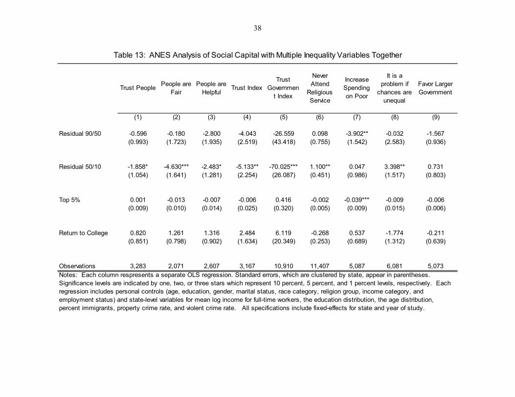
38

Trust PeoplePeople are

FairPeople are

HelpfulTrust Index

Trust Governmen

t Index

Never Attend

Religious Service

Increase Spending on Poor

It is a problem if

chances are unequal

Favor Larger Government

(1) (2) (3) (4) (5) (6) (7) (8) (9)

Residual 90/50 -0.596 -0.180 -2.800 -4.043 -26.559 0.098 -3.902** -0.032 -1.567(0.993) (1.723) (1.935) (2.519) (43.418) (0.755) (1.542) (2.583) (0.936)

Residual 50/10 -1.858* -4.630*** -2.483* -5.133** -70.025*** 1.100** 0.047 3.398** 0.731(1.054) (1.641) (1.281) (2.254) (26.087) (0.451) (0.986) (1.517) (0.803)

Top 5% 0.001 -0.013 -0.007 -0.006 0.416 -0.002 -0.039*** -0.009 -0.006(0.009) (0.010) (0.014) (0.025) (0.320) (0.005) (0.009) (0.015) (0.006)

Return to College 0.820 1.261 1.316 2.484 6.119 -0.268 0.537 -1.774 -0.211(0.851) (0.798) (0.902) (1.634) (20.349) (0.253) (0.689) (1.312) (0.639)

Observations 3,283 2,071 2,607 3,167 10,910 11,407 5,087 6,081 5,073

Table 13: ANES Analysis of Social Capital with Multiple Inequality Variables Together

Notes: Each column respresents a separate OLS regression. Standard errors, which are clustered by state, appear in parentheses. Significance levels are indicated by one, two, or three stars which represent 10 percent, 5 percent, and 1 percent levels, respectively. Each regression includes personal controls (age, education, gender, marital status, race category, religion group, income category, and employment status) and state-level variables for mean log income for full-time workers, the education distribution, the age distribution, percent immigrants, property crime rate, and violent crime rate. All specifications include fixed-effects for state and year of study.

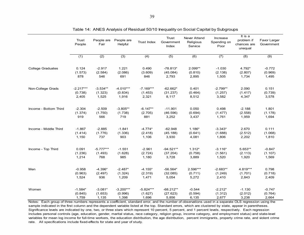
39

Trust People

People are Fair

People are Helpful

Trust IndexTrust

Government Index

Never Attend Religious Service

Increase Spending on

Poor

It is a problem if

chances are unequal

Favor Larger Government

(1) (2) (3) (4) (5) (6) (7) (8) (9)

College Graduates 0.124 -2.917 1.221 0.490 -78.813* 2.099** -1.030 4.792* -0.772(1.573) (2.584) (2.086) (3.609) (45.084) (0.810) (2.138) (2.807) (0.969)

878 546 691 846 2,793 2,895 1,505 1,734 1,495

Non-College Grads -2.217*** -3.534** -4.010*** -7.169*** -62.662* 0.401 -2.799** 2.090 0.151(0.738) (1.323) (0.834) (1.453) (31.237) (0.464) (1.257) (1.417) (0.739)2,405 1,525 1,916 2,321 8,117 8,512 3,582 4,347 3,578

Income - Bottom Third -2.304 -2.509 -3.805** -6.147** -11.901 0.050 0.498 -2.188 1.801(1.374) (1.750) (1.738) (2.705) (46.596) (0.694) (1.477) (2.558) (1.178)

919 566 719 881 3,252 3,437 1,761 1,959 1,694

Income - Middle Third -1.867 -2.885 -1.841 -4.774* -62.948 1.186* -3.343* 2.670 0.111(1.414) (1.776) (1.336) (2.418) (45.188) (0.641) (1.688) (2.512) (1.068)1,150 737 903 1,106 3,930 4,081 1,806 2,202 1,810

Income - Top Third 0.091 -5.777*** -1.551 -2.961 -94.521** 1.312* -3.116* 5.653** -0.847(1.236) (1.493) (1.628) (2.724) (37.204) (0.758) (1.561) (2.113) (1.107)1,214 768 985 1,180 3,728 3,889 1,520 1,920 1,569

Men -0.958 -4.396* -2.487* -4.155* -56.564* 2.596*** -2.683** 4.819*** 0.798(0.963) (2.497) (1.324) (2.319) (32.085) (0.711) (1.249) (1.701) (0.718)1,524 936 1,209 1,471 5,054 5,272 2,410 2,843 2,409

Women -1.584* -3.081* -3.200*** -5.824*** -68.212** -0.544 -2.212* -1.130 -0.747(0.845) (1.653) (0.996) (1.627) (27.623) (0.594) (1.312) (2.012) (0.764)1,759 1,135 1,398 1,696 5,856 6,135 2,677 3,238 2,664

Table 14: ANES Analysis of Residual 50/10 Inequality on Social Capital by Subgroups

Notes: Each group of three numbers represents a coefficient, standard error, and the number of observations used in a separate OLS regression using the sample indicated in the first column and the dependent variable listed at the top. Standard errors, which are clustered by state, appear in parentheses. Significance levels are indicated by one, two, or three stars which represent 10 percent, 5 percent, and 1 percent levels, respectively. Each regression includes personal controls (age, education, gender, marital status, race category, religion group, income category, and employment status) and state-level variables for mean log income for full-time workers, the education distribution, the age distribution, percent immigrants, property crime rate, and violent crime rate. All specifications include fixed-effects for state and year of study.

40

Trust PeoplePeople are

FairPeople are

HelpfulTrust Index

Trust Governmen

t Index

Never Attend

Religious Service

Increase Spending on Poor

It is a problem if

chances are unequal

Favor Larger

Government

(1) (2) (3) (4) (5) (6) (7) (8) (9)

College Graduates -0.691 -5.517** -2.321 -6.166 -144.045** 2.185 -4.281 0.988 -2.894(2.116) (2.223) (2.724) (4.961) (57.620) (1.403) (3.726) (5.043) (1.927)

878 546 691 846 2,793 2,895 1,505 1,734 1,495

Non-College Grads -1.395 -1.376 -4.491** -6.804*** -18.482 0.099 -6.289*** 2.003 -1.091(0.928) (1.459) (2.057) (2.219) (49.136) (0.749) (1.628) (2.247) (1.009)2,405 1,525 1,916 2,321 8,117 8,512 3,582 4,347 3,578

Income - Bottom Third -1.955 -2.635 -4.535 -6.600 -16.762 -0.840 -0.283 2.025 -0.768(2.095) (2.331) (3.120) (4.651) (66.557) (1.204) (2.217) (4.199) (1.367)

919 566 719 881 3,252 3,437 1,761 1,959 1,694

Income - Middle Third 0.035 -0.301 -5.267* -4.747 -13.705 1.111 -10.288*** 0.531 0.162(2.045) (1.905) (2.774) (3.933) (54.871) (0.924) (1.881) (4.133) (1.421)1,150 737 903 1,106 3,930 4,081 1,806 2,202 1,810

Income - Top Third -2.588 -5.087** -2.024 -8.302** -122.171** 1.166 -4.344 -1.542 -1.608(1.623) (2.245) (2.586) (3.784) (52.850) (1.155) (3.210) (3.433) (1.816)1,214 768 985 1,180 3,728 3,889 1,520 1,920 1,569

Men -2.041 -2.285 -4.463** -6.093* -89.930* 2.112** -6.701*** 1.741 -1.481(1.495) (2.340) (2.037) (3.440) (49.153) (0.852) (2.000) (3.488) (1.260)1,524 936 1,209 1,471 5,054 5,272 2,410 2,843 2,409

Women -0.576 -2.899* -3.362 -6.172** -22.036 -0.773 -5.308** -0.882 -1.659(1.007) (1.719) (2.476) (2.738) (38.838) (0.820) (2.226) (2.860) (1.133)1,759 1,135 1,398 1,696 5,856 6,135 2,677 3,238 2,664

Table 15: ANES Analysis of Residual 90/50 Inequality on Social Capital by Subgroups

Notes: Each group of three numbers represents a coefficient, standard error, and the number of observations used in a separate OLS regression using the sample indicated in the first column and the dependent variable listed at the top. Standard errors, which are clustered by state, appear in parentheses. Significance levels are indicated by one, two, or three stars which represent 10 percent, 5 percent, and 1 percent levels, respectively. Each regression includes personal controls (age, education, gender, marital status, race category, religion group, income category, and employment status) and state-level variables for mean log income for full-time workers, the education distribution, the age distribution, percent immigrants, property crime rate, and violent crime rate. All specifications include fixed-effects for state and year of study.

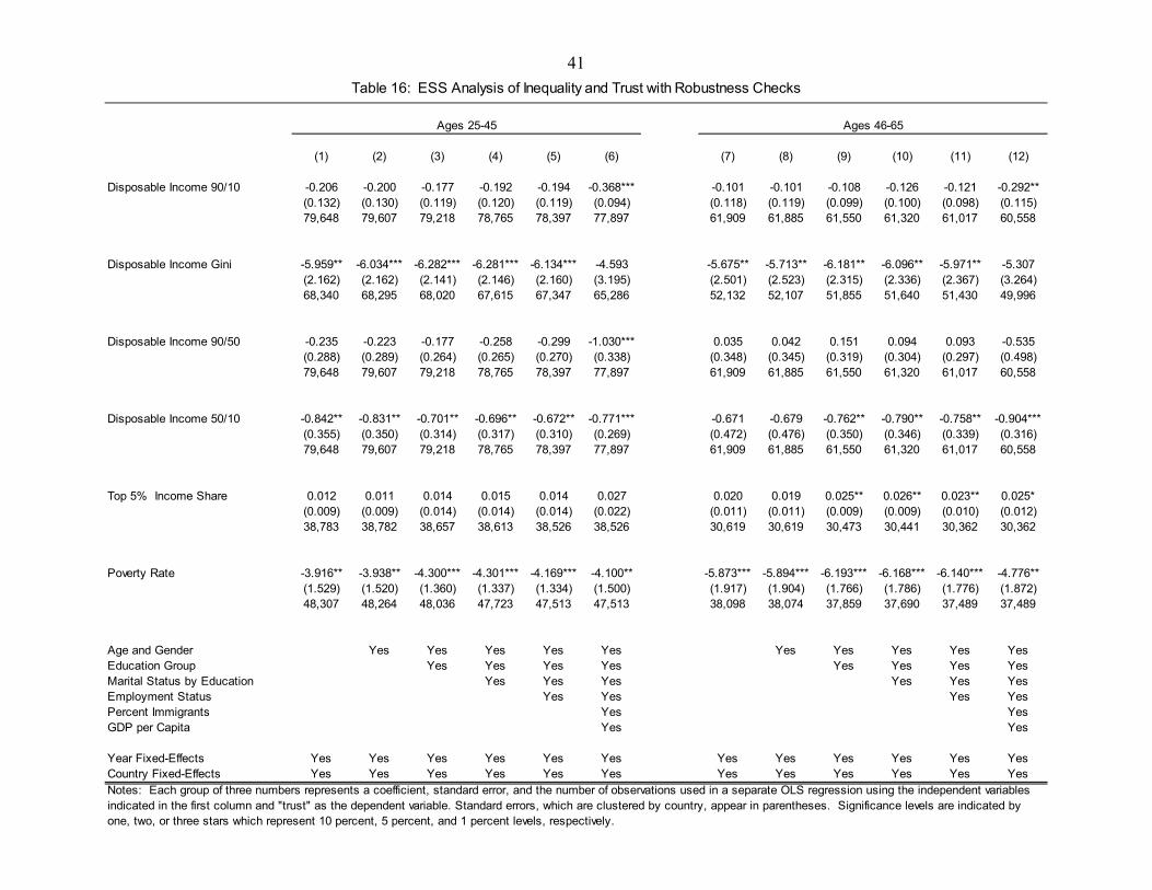
41

(1) (2) (3) (4) (5) (6) (7) (8) (9) (10) (11) (12)

Disposable Income 90/10 -0.206 -0.200 -0.177 -0.192 -0.194 -0.368*** -0.101 -0.101 -0.108 -0.126 -0.121 -0.292**(0.132) (0.130) (0.119) (0.120) (0.119) (0.094) (0.118) (0.119) (0.099) (0.100) (0.098) (0.115)79,648 79,607 79,218 78,765 78,397 77,897 61,909 61,885 61,550 61,320 61,017 60,558

Disposable Income Gini -5.959** -6.034*** -6.282*** -6.281*** -6.134*** -4.593 -5.675** -5.713** -6.181** -6.096** -5.971** -5.307(2.162) (2.162) (2.141) (2.146) (2.160) (3.195) (2.501) (2.523) (2.315) (2.336) (2.367) (3.264)68,340 68,295 68,020 67,615 67,347 65,286 52,132 52,107 51,855 51,640 51,430 49,996

Disposable Income 90/50 -0.235 -0.223 -0.177 -0.258 -0.299 -1.030*** 0.035 0.042 0.151 0.094 0.093 -0.535(0.288) (0.289) (0.264) (0.265) (0.270) (0.338) (0.348) (0.345) (0.319) (0.304) (0.297) (0.498)79,648 79,607 79,218 78,765 78,397 77,897 61,909 61,885 61,550 61,320 61,017 60,558

Disposable Income 50/10 -0.842** -0.831** -0.701** -0.696** -0.672** -0.771*** -0.671 -0.679 -0.762** -0.790** -0.758** -0.904***(0.355) (0.350) (0.314) (0.317) (0.310) (0.269) (0.472) (0.476) (0.350) (0.346) (0.339) (0.316)79,648 79,607 79,218 78,765 78,397 77,897 61,909 61,885 61,550 61,320 61,017 60,558

Top 5% Income Share 0.012 0.011 0.014 0.015 0.014 0.027 0.020 0.019 0.025** 0.026** 0.023** 0.025*(0.009) (0.009) (0.014) (0.014) (0.014) (0.022) (0.011) (0.011) (0.009) (0.009) (0.010) (0.012)38,783 38,782 38,657 38,613 38,526 38,526 30,619 30,619 30,473 30,441 30,362 30,362

Poverty Rate -3.916** -3.938** -4.300*** -4.301*** -4.169*** -4.100** -5.873*** -5.894*** -6.193*** -6.168*** -6.140*** -4.776**(1.529) (1.520) (1.360) (1.337) (1.334) (1.500) (1.917) (1.904) (1.766) (1.786) (1.776) (1.872)48,307 48,264 48,036 47,723 47,513 47,513 38,098 38,074 37,859 37,690 37,489 37,489

Age and Gender Yes Yes Yes Yes Yes Yes Yes Yes Yes YesEducation Group Yes Yes Yes Yes Yes Yes Yes YesMarital Status by Education Yes Yes Yes Yes Yes YesEmployment Status Yes Yes Yes YesPercent Immigrants Yes YesGDP per Capita Yes Yes

Year Fixed-Effects Yes Yes Yes Yes Yes Yes Yes Yes Yes Yes Yes YesCountry Fixed-Effects Yes Yes Yes Yes Yes Yes Yes Yes Yes Yes Yes Yes

Table 16: ESS Analysis of Inequality and Trust with Robustness Checks

Ages 25-45 Ages 46-65

Notes: Each group of three numbers represents a coefficient, standard error, and the number of observations used in a separate OLS regression using the independent variables indicated in the first column and "trust" as the dependent variable. Standard errors, which are clustered by country, appear in parentheses. Significance levels are indicated by one, two, or three stars which represent 10 percent, 5 percent, and 1 percent levels, respectively.

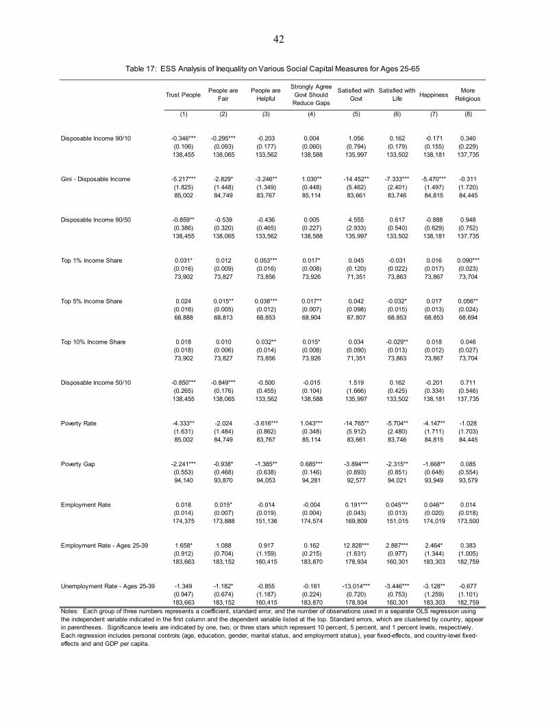
42

Trust PeoplePeople are

FairPeople are

Helpful

Strongly Agree Govt Should

Reduce Gaps

Satisfied with Govt

Satisfied with Life

HappinessMore

Religious

(1) (2) (3) (4) (5) (6) (7) (8)

Disposable Income 90/10 -0.346*** -0.295*** -0.203 0.004 1.056 0.162 -0.171 0.340(0.106) (0.093) (0.177) (0.060) (0.794) (0.179) (0.155) (0.229)138,455 138,065 133,562 138,588 135,997 133,502 138,181 137,735

Gini - Disposable Income -5.217*** -2.829* -3.246** 1.030** -14.452** -7.333*** -5.470*** -0.311(1.825) (1.448) (1.349) (0.448) (5.462) (2.401) (1.497) (1.720)85,002 84,749 83,767 85,114 83,661 83,746 84,815 84,445

Disposable Income 90/50 -0.859** -0.539 -0.436 0.005 4.555 0.617 -0.888 0.948(0.386) (0.320) (0.465) (0.227) (2.933) (0.540) (0.629) (0.752)138,455 138,065 133,562 138,588 135,997 133,502 138,181 137,735

Top 1% Income Share 0.031* 0.012 0.053*** 0.017* 0.045 -0.031 0.016 0.090***(0.016) (0.009) (0.016) (0.008) (0.120) (0.022) (0.017) (0.023)73,902 73,827 73,856 73,926 71,351 73,863 73,867 73,704

Top 5% Income Share 0.024 0.015** 0.038*** 0.017** 0.042 -0.032* 0.017 0.056**(0.016) (0.005) (0.012) (0.007) (0.098) (0.015) (0.013) (0.024)68,888 68,813 68,853 68,904 67,807 68,853 68,853 68,694

Top 10% Income Share 0.018 0.010 0.032** 0.015* 0.034 -0.029** 0.018 0.046(0.018) (0.006) (0.014) (0.008) (0.090) (0.013) (0.012) (0.027)73,902 73,827 73,856 73,926 71,351 73,863 73,867 73,704

Disposable Income 50/10 -0.850*** -0.849*** -0.500 -0.015 1.519 0.162 -0.201 0.711(0.265) (0.176) (0.455) (0.104) (1.666) (0.425) (0.334) (0.546)138,455 138,065 133,562 138,588 135,997 133,502 138,181 137,735

Poverty Rate -4.333** -2.024 -3.616*** 1.043*** -14.765** -5.704** -4.147** -1.028(1.631) (1.484) (0.862) (0.348) (5.912) (2.480) (1.711) (1.703)85,002 84,749 83,767 85,114 83,661 83,746 84,815 84,445

Poverty Gap -2.241*** -0.938* -1.385** 0.685*** -3.894*** -2.315** -1.668** 0.085(0.553) (0.468) (0.638) (0.146) (0.893) (0.851) (0.648) (0.554)94,140 93,870 94,053 94,281 92,577 94,021 93,949 93,579

Employment Rate 0.018 0.015* -0.014 -0.004 0.191*** 0.045*** 0.046** 0.014(0.014) (0.007) (0.019) (0.004) (0.043) (0.013) (0.020) (0.018)174,375 173,888 151,136 174,574 169,809 151,015 174,019 173,500

Employment Rate - Ages 25-39 1.658* 1.088 0.917 0.162 12.828*** 2.887*** 2.464* 0.383(0.912) (0.704) (1.159) (0.215) (1.631) (0.977) (1.344) (1.005)183,663 183,152 160,415 183,870 178,934 160,301 183,303 182,759

Unemployment Rate - Ages 25-39 -1.349 -1.182* -0.855 -0.181 -13.014*** -3.446*** -3.128** -0.677(0.947) (0.674) (1.187) (0.224) (0.720) (0.753) (1.259) (1.101)183,663 183,152 160,415 183,870 178,934 160,301 183,303 182,759

Table 17: ESS Analysis of Inequality on Various Social Capital Measures for Ages 25-65

Notes: Each group of three numbers represents a coefficient, standard error, and the number of observations used in a separate OLS regression using the independent variable indicated in the first column and the dependent variable listed at the top. Standard errors, which are clustered by country, appear in parentheses. Significance levels are indicated by one, two, or three stars which represent 10 percent, 5 percent, and 1 percent levels, respectively. Each regression includes personal controls (age, education, gender, marital status, and employment status), year fixed-effects, and country-level fixed-effects and and GDP per capita.

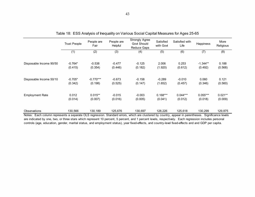
43

Trust PeoplePeople are

FairPeople are

Helpful

Strongly Agree Govt Should

Reduce Gaps

Satisfied with Govt

Satisfied with Life

HappinessMore

Religious

(1) (2) (3) (4) (5) (6) (7) (8)

Disposable Income 90/50 -0.764* -0.538 -0.477 -0.125 2.006 0.253 -1.344** 0.188(0.415) (0.354) (0.446) (0.182) (1.920) (0.612) (0.492) (0.568)

Disposable Income 50/10 -0.705* -0.770*** -0.673 -0.158 -0.289 -0.010 0.060 0.121(0.342) (0.198) (0.525) (0.147) (1.652) (0.457) (0.346) (0.560)

Employment Rate 0.012 0.015** -0.015 -0.003 0.168*** 0.044*** 0.055*** 0.021**(0.014) (0.007) (0.016) (0.005) (0.041) (0.012) (0.018) (0.009)

Observations 130,566 130,189 125,676 130,697 128,226 125,618 130,299 129,875

Table 18: ESS Analysis of Inequality on Various Social Capital Measures for Ages 25-65

Notes: Each column represents a separate OLS regression. Standard errors, which are clustered by country, appear in parentheses. Significance levels are indicated by one, two, or three stars which represent 10 percent, 5 percent, and 1 percent levels, respectively. Each regression includes personal controls (age, education, gender, marital status, and employment status), year fixed-effects, and country-level fixed-effects and and GDP per capita.

44

Trust PeoplePeople are

FairPeople are

Helpful

Strongly Agree Govt Should

Reduce Gaps

Satisfied with Govt

Satisfied with Life

HappinessMore

Religious

(1) (2) (3) (4) (5) (6) (7) (8)

College Graduates -0.370*** -0.460*** -0.238 -0.040 1.501 0.052 -0.081 0.413*(0.098) (0.097) (0.143) (0.059) (0.918) (0.173) (0.175) (0.227)39,413 39,351 37,949 39,432 38,991 37,936 39,336 39,225

Non College Graduates -0.324** -0.232** -0.191 0.009 0.895 0.191 -0.173 0.272(0.130) (0.108) (0.215) (0.065) (0.779) (0.202) (0.157) (0.244)99,042 98,714 95,613 99,156 97,006 95,566 98,845 98,510

Men -0.306** -0.325** -0.219 0.006 1.099 0.096 -0.193 0.351(0.132) (0.141) (0.204) (0.052) (0.871) (0.182) (0.158) (0.254)66,008 65,858 63,774 66,083 65,112 63,755 65,881 65,642

Women -0.375** -0.263*** -0.185 0.003 1.015 0.211 -0.162 0.317(0.143) (0.084) (0.188) (0.069) (0.737) (0.203) (0.160) (0.238)72,447 72,207 69,788 72,505 70,885 69,747 72,300 72,093

Table 19: ESS Analysis of 90/10 Inequality on Various Social Capital Measures within Subgroups for Ages 25-65

Notes: Each group of three numbers represents a coefficient, standard error, and the number of observations used in a separate OLS regression. Standard errors, which are clustered by country, appear in parentheses. Significance levels are indicated by one, two, or three stars which represent 10 percent, 5 percent, and 1 percent levels, respectively. Each regression includes personal controls (age, education, gender, marital status, and employment status), year fixed-effects, and country-level fixed-effects and and GDP per capita.

45

Trust PeoplePeople are

FairPeople are

Helpful

Strongly Agree Govt Should

Reduce Gaps

Satisfied with Govt

Satisfied with Life

HappinessMore

Religious

(1) (2) (3) (4) (5) (6) (7) (8)

College Graduates -1.000*** -0.828*** -0.717 -0.102 1.721 -0.085 -0.016 0.794(0.325) (0.282) (0.486) (0.096) (1.983) (0.480) (0.397) (0.529)39,413 39,351 37,949 39,432 38,991 37,936 39,336 39,225

Non College Graduates -0.793** -0.836*** -0.435 0.004 1.392 0.201 -0.208 0.704(0.356) (0.222) (0.514) (0.119) (1.655) (0.480) (0.345) (0.629)99,042 98,714 95,613 99,156 97,006 95,566 98,845 98,510

Men -0.845** -0.777** -0.596 -0.033 1.716 0.013 -0.182 0.541(0.306) (0.313) (0.455) (0.108) (1.690) (0.484) (0.332) (0.467)66,008 65,858 63,774 66,083 65,112 63,755 65,881 65,642

Women -0.847** -0.902*** -0.404 0.005 1.332 0.269 -0.246 0.822(0.361) (0.224) (0.554) (0.126) (1.668) (0.420) (0.361) (0.717)72,447 72,207 69,788 72,505 70,885 69,747 72,300 72,093

Table 20: ESS Analysis of 50/10 Inequality on Various Social Capital Measures within Subgroups for Ages 25-65

Notes: Each group of three numbers represents a coefficient, standard error, and the number of observations used in a separate OLS regression. Standard errors, which are clustered by country, appear in parentheses. Significance levels are indicated by one, two, or three stars which represent 10 percent, 5 percent, and 1 percent levels, respectively. Each regression includes personal controls (age, education, gender, marital status, and employment status), year fixed-effects, and country-level fixed-effects and and GDP per capita.

46

Trust PeoplePeople are

FairPeople are

Helpful

Strongly Agree Govt Should

Reduce Gaps

Satisfied with Govt

Satisfied with Life

HappinessMore

Religious

(1) (2) (3) (4) (5) (6) (7) (8)

College Graduates -0.774 -1.411*** -0.312 -0.134 6.420** 0.409 -0.463 1.027(0.476) (0.365) (0.274) (0.219) (2.775) (0.431) (0.469) (0.677)39,413 39,351 37,949 39,432 38,991 37,936 39,336 39,225

Non College Graduates -0.805* -0.239 -0.455 0.020 3.898 0.708 -0.916 0.649(0.401) (0.333) (0.619) (0.236) (2.967) (0.622) (0.697) (0.806)99,042 98,714 95,613 99,156 97,006 95,566 98,845 98,510

Men -0.745 -0.735 -0.466 0.031 4.439 0.404 -0.999 1.160(0.517) (0.472) (0.555) (0.200) (3.180) (0.583) (0.593) (0.876)66,008 65,858 63,774 66,083 65,112 63,755 65,881 65,642

Women -0.930* -0.338 -0.392 -0.015 4.655 0.802 -0.794 0.731(0.484) (0.268) (0.555) (0.251) (2.735) (0.610) (0.666) (0.698)72,447 72,207 69,788 72,505 70,885 69,747 72,300 72,093

Table 21: ESS Analysis of 90/50 Inequality on Various Social Capital Measures within Subgroups for Ages 25-65

Notes: Each group of three numbers represents a coefficient, standard error, and the number of observations used in a separate OLS regression. Standard errors, which are clustered by country, appear in parentheses. Significance levels are indicated by one, two, or three stars which represent 10 percent, 5 percent, and 1 percent levels, respectively. Each regression includes personal controls (age, education, gender, marital status, and employment status), year fixed-effects, and country-level fixed-effects and and GDP per capita.