groundwater salinity modeling using artificial neural networks · iii abstract the main source of...
TRANSCRIPT

غزةبالجامعة اإلسالمية
عمادة الدراسات العليا
ندسـةـة الهـآلي
قسم الهندسة المدنية
مصادر المياههندسة
The Islamic University of Gaza
High Studies Deanery
Faculty of Engineering
Civil Engineering Department
Water Resources Engineering
Groundwater Salinity Modeling
Using Artificial Neural Networks
Gaza Strip case study
Submitted By
Eng. Mohammed Seyam
Supervised By
Dr. Yunes Mogheir
A Thesis Submitted in Partial Fulfillment of the Requirement for the
Degree of Master of Science in Civil/ Water Resources Engineering
- 2009م 1430 هـ

II
بسم اهللا الرحمن الرحيم
رب أوزعين أن أشكر �عمتك اليت أ�عمت علـي وعلـى والـدي وأن أعمـل صـاحلا ترضـاه { }برمحتك يف عبادك الصاحلنيوأدخلين
)19 النمل اآلية (
“O my Lord! So order me that I may be grateful for Thy favours, which Thou has bestowed
on me and on my parents, and that I may work the righteousness that will please Thee: and
admit me, by Thy Grace, to the ranks of Thy Righteous Servants”
III
Abstract
The main source of water in Gaza Strip is the shallow aquifer which is part of the coastal aquifer. The quality of the groundwater is extremely deteriorated in terms of salinity. Salinization of groundwater may be caused and influenced by many variables. Studying the relation of between these variables and salinity is often a complex and nonlinear process, making it suitable for Artificial Neural Networks (ANN) application.
In order to model groundwater salinity in Gaza Strip using ANN it is necessary to gather data for training purposes. Initially, it is assumed that the groundwater salinity (represented by chloride concentration, mg/l) may be affected by some variables as: recharge rate (R), abstraction (Q), abstraction average rate (Qr), life time (Lt), groundwater level Wl, aquifer thickness (Th), depth from surface to well screen (Dw), and distance from sea shore line (Ds). Data were extracted from 56 wells, most of them are municipal wells and they almost cover the total area of Gaza Strip.
The initial modeling trials were made using all input variables and many trials were applied to get best performance model. From the created ANN models, the importance and effect of each variables was studied and represented, also depending on the results of ANN models some input variables were neglected and new modeling trials are made without using neglected input variables.
After a number of trials, the best neural network was determined to be Multilayer Perceptron network (MLP) with four layers: an input layer of 6 neurons, first hidden layer with 10 neurons, second hidden layer with 7 neurons and the output layer with 1 neuron. The six input neurons are: initial chloride concentration (Clo), recharge rate (R), abstraction (Q), abstraction average rate of area (Qr), life time (Lt), aquifer thickness (Th). The output neuron gives the final chloride concentration (Clf).
The ANN model generated very good results depending on the high correlation between the observed and simulated values of chloride concentration. The correlation coefficient (r) was 0.9848. The high value of (r) showed that the simulated chloride concentration values using the ANN model were in very good agreement with the observed chloride concentration which mean that ANN model is useful and applicable for groundwater salinity modeling. ANN model was successfully utilized as analytical tool to study influence of the input variables on chloride concentration. It proved that chloride concentration in groundwater is directly affected by abstraction (Q), abstraction average rate (Qr) and life time (Lt). Furthermore, it was adversely affected by recharge rate (R) and aquifer thickness (Th). Furthermore, it is utilized as simulation and prediction tool of chloride concentration in domestic wells in Gaza Strip, the prediction of chloride concentration will be based on some scenarios of abstraction from groundwater. Also it will be used as a decision making support tool that suggests the appropriate abstraction from groundwater wells comparing with the status of salinity.

IV
الخالصـة
ق تعتبر المياه الجوفية المصدر الرئيسي للمياه في ق ا يتعل وث وخصوصًا فيم طاع غزة و هي معرضة للتل
ذه دراسة إن.متغيراتالبازدياد معدالت الملوحة التي تتواجد وتتأثر بالعديد من ين ه رات العالقة ب و الملوحة المتغي
. من خالل الشبكات العصبية الصناعية و تنمذج ما تكون عملية معقدة مما يجلها مناسبة لتدرسعادًة
ة إن نمذجة مل ة لعملي وحة المياه الجوفية من خالل الشبكات العصبية الصناعية تتطلب جمع البيانات الالزم
د . التدريب التي تقوم بها الشبكة العصبية ة الكلوري ة بكمي ة المتمثل اه الجوفي في البداية أفترض البحث أن ملوحة المي
ا متغيراتبعدة في المياه الجوفية تتأثر سحب الخاصة بكل هي معدل تسرب مياه األمط ة ال ر للخزان الجوفي و آمي
اه سوب المي سحب و من ا الخزان الجوفي لل ي تعرض فيه ة الت بئر ومعدل السحب من الخزان الجوفي و المدة الزمني
سحب و البحر سطح األرض عن الخزان الجوفي عمق الجوفية و سمك الخزان الجوفي و ة ال ين منطق سافة ب و الم
. بئر مياه تغطي معظم مساحة قطاع غزة56نات من ولقد استخرجت هذه البيا
د المفترضة متغيراتالفي البداية تمت عملية النمذجة باستخدام جميع ذ عدة محاوالت للحصول وق م تنفي ت
اه على نموذج يعطى نتائج جيدة و من النماذج التي تم تطويرها تم دراسة تأثير العوامل على ترآيز الكلوريد في المي
ا أن الجوفية ين من خالله م عمل محاوالت أخرى تب و بناء على الدراسة تبين أنه يمكن تجاهل بعض العوامل و ت
ا هي م التوصل إليه ع Multilayer Perceptron network (MLP)أفضل شبكة عصبية ت و تتكون من أرب
ا 6طبقات هي طبقة المدخالت و يوجد بها ة 10 نيورن و الطبقة المخفية األولى و يوجد به ة المخفي ورن و الطبق ني
ز . نيورن وطبقة المخرجات و يوجد بها نيرون واحد 7الثانية و يوجد بها ة ترآي طبقة المدخالت تمثل العوامل التالي
سحب من الكلوريد االبتدائي و معدل تسرب مياه األمطار للخزان الجوفي و آمية السحب الخاصة بكل بئر ومعدل ال
دة ا وفي و الم زان الج ة الخ ا طبق وفي أم زان الج مك الخ سحب و س وفي لل زان الج ا الخ رض فيه ي تع ة الت لزمني
.المخرجات فتمثل ترآيز الكلوريد النهائي
يم المستخرجة ة و الق يم الحقيق ين الق لقد أعطت الشبكة العصبية نتائج ممتازة اعتمادًا على التقارب الكبير ب
يم 9848.0 من النموذج حيث بلغت قيمة معامل االرتباط ة و الق يم الحقيق ين الق رًا ب ا آبي اك توافق ي أن هن ذا يعن و ه
ق أداة لدراسة . المستخرجة من النموذج مما يجعل النموذج صالحًا لالستخدام و التطبي م استخدام النموذج بنجاح آ ت
سحب ا ة ال ر تأثير العوامل على ترآيز الكلوريد حيث تبين أن ترآيز الكلوريد يتناسب طرديًا مع آمي لخاصة بكل بئ
سيًا ا تتناسب عك سحب و أنه ومعدل السحب من الخزان الجوفي و المدة الزمنية التي تعرض فيها الخزان الجوفي لل
ز ؤ بترآي يلة للتنب وذج آوس تخدم النم اه األمطار للخزان الجوفي و سمك الخزان الجوفي واس سرب مي دل ت ع مع م
ا استخدم النموذج الكلوريد لعدة سيناريوهات تدرس تأثير السحب من ستقبل آم الخزان الجوفي على الملوحة في الم
. ثابتة في آل بئر على حدةهاآأداة لتحديد آمية السحب المسموح بها لتحسين الملوحة أو الحفاظ علي

V
Dedication
Proudly, I dedicate my thesis to my parents, as I always feel their prayers in
all aspects of my life, my beloved brothers, sisters, friends, colleagues.
Finally special dedication to my wife Aisha and my lovely sons Adnan and
Ibraheem.

VI
Acknowledgements
First and foremost, I am grateful to my lord who has given me the strength, enablement,
wisdom, knowledge and required understanding to complete this thesis.
Next, I wish to express my unreserved gratitude to my advisor, Dr. Yunes Mogheir, for
his help. His constructive criticisms and ideas have made this project worth reading. To
say am very privileged to have him as my advisor.
I will also like to extend my sincere appreciation to Dr. Mohammed Arafa and Dr.
Mamoun Alqedra since they give me first knowledge about ANN during Bachelors
studying.
I would like to thank the Islamic University of Gaza, Faculty of Engineering for
providing me high standard of Education through the duration of a master program of
Water Recourses Engineering.
I appreciate the support rendered by the staff of PWA and CMWU. They made the data
used in this project available.
I would like to thank all those who have assisted, guided and supported me in my
studies leading to this thesis.
Finally, I would like to extend my deepest gratitude to parents and my wife, they have
always given me unremitting support during preparation my thesis.

VII
Table of Contents
PageItem
iii Abstract v Dedication vi Acknowledgements vii Table of Contents xi List of Tables xiii List of Figures xvii List of Abbreviations xviii Units and measures 1 Chapter (1) Introduction 1 Background 1.1 2 Statement of the Problem 1.2 3 Objectives 1.3 3 Methodology 1.4 3 Thesis Outline 1.5 5 Chapter (2) Literature Review / Groundwater Salinity 5 Introduction 2.1 5 Physico-chemical Properties of Salinity of Groundwater 2.2 6 The Effects of Groundwater Salinity 2.3 6 Sources of Groundwater 2.4 7 Naturally Occurring Groundwater 2.4.1 7 Sea Water 2.4.1.1 7 Geothermal 2.4.1.2 7 Pollutants Originated From Geological 2.4.1.3 7 Groundwater Pollution Produced by Human 2.4.2 7 Municipal 2.4.2.1 7 Industrial 2.4.2.2 7 Agricultural 2.4.2.2 8 Groundwater Salinity in Gaza 2.5 9 Groundwater 2.6 9 Groundwater Modeling in Gaza Strip 2.6.1 12 Chapter (3) Literature Review/Artificial Neural Networks 12 Introduction to Artificial Neural Networks 3.1 14 History of Artificial Neural Networks 3.2 15 Architectures of Artificial Neural Network 3.3 15 Simple Neuron (a single scalar input) 3.3.1 15 Neuron without bias 3.3.1.1 15 Neuron with bias 3.3.1.2 16 Neuron with Vector Input 3.3.2 16 Layers of neurons 3.3.3 16 Perceptron Network 3.3.3.1 17 Multiple Layers of Neurons 3.3.3.2

VIII
PageItem
18 Artificial Neural Networks Learning 3.4 18 Types of Artificial Neural Networks 3.5 19 The Back Propagation (BP) Method 3.5.1 20 The Radial Basis Function-Based Neural Networks (RBF) 3.5.2 21 Building Artificial Neural Networks 3.6 22 Artificial Neural Networks Aِpplications in Hydrology Fields 3.7 23 Artificial Neural Networks applications in Groundwater Quality
Modeling 3.8
25 Chapter (4) Study Area Description 25 Location and Population 4.1 25 Topography 4.2 27 Climate and Rainfall 4.3 27 Climate 4.3.1 27 Rainfall 4.3.2 28 Land Use 4.4 30 Geology 4.5 31 Tertiary Formation 4.5.1 31 Quaternary Formation 4.5.2 31 Marine Kurkar Formation 4.5.2.1 31 Continental Kurkar Formation 4.5.2.2 31 Quaternary Deposits 4.5.2.3 32 Soil Condition 4.6 32 Subsoil Formation 4.6.1 32 Kurkar 4.6.1.1 32 Hamra 4.6.1.2 32 Soil Formation 4.6.2 34 Hydrology 4.7 34 Surface Water Hydrology 4.7.1 35 Groundwater Hydrology 4.7.2 35 Hydrostratigraphy 4.7.2.l 47 Aquifer Hydraulic Properties 4.7.3 36 Transmissivity 4.7.3.1 36 Effective Porosity: 4.7.3.2 37 Specific Yield and Specific Storativity 4.7.3.3 37 Groundwater Balance 4.7.4 39 Chapter (5) Methodology 39 Introduction 5.1 39 Data Collection and Preparation 5.2 40 Water Wells in Study Area 4.2.1 41 Chloride Concentration Data 5.2.2 42 Recharge Rate 5.2.3 42 Factors Influence Infiltration Rate 5.2.3.1 45 Computation Methods of Infiltration 5.2.3.2

IX
PageItem
46 Computation of Recharge in Gaza Strip 5.2.3.3 47 Procedures for Calculation of Recharge Rate of Study Wells 5.2.3.4 49 Abstraction 5.2.4 49 Agricultural Abstraction 5.2.4.1 49 Municipal Wells Abstraction 5.2.4.2 50 Distance From Sea Shore Line 5.2.5 52 Water Level Data 5.2.6 53 Depth from ground surface to well screen 5.2.7 53 Saturated Aquifer Thickness 5.2.8 53 Lithological Cross Sections 5.2.8.1 54 Determination Aquifer Thickness of each Study Wells 5.2.8.2 58 Construction data matrix for ANN Model 5.3 58 Selection the Variables of ANN Model 5.3.1 58 Time Distribution Phases of ANN Model Data 5.3.2 59 Organizing of ANN Model Data 5.3.3 61 Analysis of ANN Model Data 5.3.4 64 Procedural Steps in Building ANN Model 5.4 64 Data Importation 5.4.1 64 Problem Definition 5.4.2 64 Extraction of the Test Set 5.4.3 65 Network Design 5.4.4 65 Network Training 5.4.5 65 Network Calibration 5.4.6 65 Calibration Based on Best Test Set 5.4.6.1 65 Calibration Based on Minimum Error Events 5.4.6.2 66 Testing of Network 5.4.7 67 Chapter (6) Results and Discussions 67 Introduction 6.1 67 Characters of Initial ANN Model 6.2 67 Topology of ANN 6.2.1 67 Performance of ANN 6.2.2 70 Regression Statistics of ANN Model 6.2.3 72 Response Presentations 6.2.4 74 Sensitivity Analysis 6.2.5 75 Determination the Real Importance of Input Variables 6.2.6 75 Characters of the Final ANN Model 6.3 75 Topology of the ANN 6.3.1 78 Performance of ANN 6.3.2 80 Regression Summary Statistics of Final ANN Model 6.3.3 81 Sensitivity analysis 6.3.4 81 Response Presentations 6.3.5 81 Response Graph 6.3.5.1

X
PageItem
84 Response surface 6.3.5.2 86 Application of ANN Model 6.4 86 Utilizing ANN Model as Analytical Tool 6.4.1 88 Impact of Recharge Rate on Chloride Concentration 6.4.1.1 91 Influence of Abstraction on Chloride Concentration 6.4.1.2 92 Impacts of Abstraction Average Rate on Chloride6.4.1.3 94 Effect of Life Time on Chloride Concentration 6.4.1.4 96 Effect of Aquifer thickness on Chloride Concentration 6.4.1.5 98 Utilizing ANN Model as a Simulation Tool 6.4.2 100 Utilizing ANN Model as a Prediction Tool 6.4.3 100 Utilizing ANN Model as Future Scenarios Prediction Tool 6.4.4 100 Scenario 1: No Change of Abstraction Condition 6.4.4.1 102 Scenario 2: The Total Abstraction Will be Reduced by Half 6.4.4.2 103 Scenario 3: No Abstraction Condition 6.4.4.2 104 Utilizing ANN Model as Decision Making Support Tool 6.4.4 106 Chapter (7) Conclusions and Recommendations 106 Conclusions 7.1 107 Recommendations 7.2 109 References 115 Annexes

XI
List of Tables
PageTitle Tables
6 Classification of water according to their content of TDS (Desjardins, 1988)……………………………………………..
Table (2.1)
25 The revised estimates of the population projection in Gaza Strip (PCBS, 2005)……………………………………………..
Table (4.1)
28 Proposed Land Use Distribution in Gaza Strip for the Year 2004 (MOLG, 2004)………………………………………….
Table (4.2)
30
Geology and Geological History of the Gaza Strip (Palestinian Environmental Protection Authority, 1994) and (Hamdan, 1999)……………………………………………………………
Table (4.3)
33
Classification & Characteristics of Different Soil Types in Gaza Strip. (Mopic, 1997; Goris and Samain, 2001)………..…………………………………………………..
Table (4.4)
37 Aquifer hydraulic properties (PWA, 2000b)…………………... Table (4.5)
37 Estimated Water Balance of the Gaza Strip ( Adopted from Metcalf and Eddy, 2007)……………………………………….
Table (4.6)
40 The general information of study wells………………………... Table (5.1)
41 Chloride concentration of some study wells from 1997 to 2000…………………………………………………………….
Table (5.2)
43
Texture and infiltration Parameters of the Different Soil Types in the Gaza Strip (Goris and Samain ,(2001), and (Hamdan, 1999)……………………………………………………………
Table (5.3)
49 Soil recharge coefficient , influence rainfall station, land use and soil type for each study wells……………………………...
Table (5.4)
51 Monthly municipal abstraction in Gaza strip for Year 2007….. Table (5.5) 50 The distance between the study wells and sea shore line……… Table (5.6) 53 The depth from surface to well screen of some study wells…... Table (5.7)
54 The Lithological cross section number, sub aquifer and saturated thickness of sub aquifer of each study wells…………
Table (5.8)
58 The variables of ANN model………………………………….. Table (5.9)
59 The time distribution phase of the ANN model for the years 1997 and 1998…………………………………………………
Table (5.10)
59 The procedures of organizing ANN model variables………….. Table (5.11) 61 Side of ANN model matrix…………………………………… Table (5.12)
62 Mean, standard deviation and ranges of variables used to train the ANN model………………………………………………...
Table (5.13)
71 The values of regression statistics for the ANN model………... Table (6.1) 75 The value of error ratio and rank of input variables…………… Table (6.2) 75 Sensitivity analysis of twenty ANN models…………………... Table (6.3)
76 Rank of ANN model variables extracted from twenty ANN models………………………………………………………….
Table (6.4)
80 The values of regression statistics for final ANN model……… Table (6.5)
81 The value of error ratio and rank of input variables…………… Table (6.6)
87 Hypothetical values of gradual change for input variables……. Table (6.7)

XII
PageTitle Tables
88 Hypothetical values of input variables for the three analysis conditions………………………………………………………
Table (6.8)
89 Results of ANN model for hypothetical cases studied the effect of recharge rate on chloride concentration……………………..
Table (6.9)
90 Summary of results of ANN model for hypothetical cases studied the effect of recharge rate on chloride concentration….
Table (6.10)
91 Results of ANN model for hypothetical cases studied the effect of abstraction on chloride concentration……………………….
Table (6.11)
93 Results of ANN model for hypothetical cases studied the effect of abstraction average rate on chloride concentration………….
Table (6.12)
95 Results of ANN model for hypothetical cases studied the effect of life time on chloride concentration………………………….
Table (6.13)
97 Results of ANN model for hypothetical cases studied the effect of aquifer thickness on chloride concentration ………………..
Table (6.14)

XIII
List of Figures
PageTitle Figure
3 Flow chart of the research methodology………………………. Figure (1.1) 8 The sources of salinity in ground water (Phillips, 2005)………. Figure (2.2)
9 Average chloride concentration of pumped groundwater of Gaza Strip for the year 2002 (PWA, 2003)……………………
Figure (2.2)
9 Average chloride concentration of pumped groundwater of Gaza Strip for the year 2007 (CMWU, 2008)…………………
Figure (2.3)
12 Mammalian neuron (Ajith, 2005)……………………………… Figure (3.1)
13 Model of artificial neurons (Hola and Schabowicz, 2005)……….……………………………………………….…..
Figure (3.2)
14 Schematic description of a three layer ANN and of the elements of its (mathematical) neurons (Claudius et al., 2005)..
Figure (3.3)
15 Neuron without bias (Matlab,1994) ………...…………………. Figure (3.4)
16 Neuron with bias (Matlab,1994) ………………………...…….. Figure (3.5)
16 Neuron with Vector Input (Matlab,1994) …………………...… Figure (3.6)
17 Perceptron network (Matlab,1994) ……….………..…………. Figure (3.7)
17 Multiple Layers of Neurons (Matlab,1994) …………………… Figure (3.8)
18 Neural Network Mechanism (Matlab,1994) ……………...…… Figure (3.9)
20 Radial Basis function Networks (Matlab,1994) ……………….. Figure (3.10)
22 A random sample of neural network…………………………… Figure (3.11)
26 Regional and location map of Gaza Strip (UNEP, 2009)……… Figure (4.1)
26 Topographical map of Gaza Strip (MOPIC, 1997)……………. Figure (4.2)
28 The rainfall depth in Gaza Strip for 2006-2007 season (PWA, 2007)…………………………………………………………….
Figure (4.3)
29 Land use in Gaza Strip (MOPIC, 1998)………………………. Figure (4.4)
29 The proposed future land use distribution in 2015) (MWGP, 2001)……………………………………………………………
Figure (4.5)
31 A geological Cross-Section in the Gaza Strip. (Metcalf and Eddy, 2000)…………………………………………………….
Figure (4.6)
33 Soil Classifications in Gaza Strip (MOPIC, 1997)…………….. Figure (4.7) 40 Study wells location in Gaza Strip……………………………... Figure (5.1) 40 Study wells and land use in Gaza Strip………………………… Figure (5.2)
41 Average chloride concentration of pumped groundwater of Gaza Strip for the year 2007 (CMWU, 2007)…………………..
Figure (5.3)
43 The study wells according to soil types of Gaza Strip…………. Figure (5.4) 44 The Soil Structure ( FAO, 1993)……………………………….. Figure (5.5) 45 The Basic Types of Soil Structures ( FAO, 1993)…………….. Figure (5.6) 48 The soil recharge coefficients for Gaza Strip (CAMP, 2000)…..Figure (5.7) 48 Rainfall thissen network for Gaza Strip catchment's area………Figure (5.8) 50 Monthly municipal abstraction in Gaza Strip for year 2007….. Figure (5.9)
52 Groundwater level contour map of Gaza Strip area for the year 2007(CMWU, 2007)………………...………………………….
Figure (5.10)
55 Lithological Cross sections for Palestine and Gaza Strip (IWA, Figure (5.11)

XIV
PageTitle Figure
1991)…………………………………………………………….
56 Lithological Cross sections number for Gaza Strip Aquifer ( IWA, 1991)…………………………………………………...
Figure (5.12.a)
56 Geological cross section number 93 (IWA, 1991)…..…………. Figure (5.12.b) 57 Geological cross section number 94 (IWA, 1991)…..…………. Figure (5.12.c) 57 Geological cross section number 95 (IWA, 1991)…..…………. Figure (5.12.d) 57 Geological cross section number 96 (IWA, 1991)…..…………. Figure (5.12.e)
62 Frequency distribution of the variables across the range of 499 cases…………………………………………………………….
Figure (5.13)
62 Frequency distribution of initial chloride concentration (Clo)…. Figure (5.13.a) 62 Frequency distribution of recharge rate (R)……………………. Figure (5.13.b) 63 Frequency distribution of abstraction (Q)……………………… Figure (5.13.c) 63 Frequency distribution of groundwater level (Wl)……………...Figure (5.13.f) 63 Frequency distribution of life time (Lt)…………………………Figure (5.13.e) 63 Frequency distribution of abstraction average rate (Qr)……….. Figure (5.13.d)
63 Frequency distribution of depth from surface to well screen (Dw)…………………………………………………………….
Figure (5.13.g)
63 Frequency distribution of aquifer thickness (Th)………………. Figure (5.13.h) 64 Frequency distribution of distance from sea shore line (Ds)…... Figure (5.13.i) 64 Frequency distribution of final chloride concentration (Clf)…... Figure (5.13.j) 68 Topology of the ANN model………………………………...… Figure (6.1) 68 Training progress of ANN………………………………………Figure (6.2)
69 Comparison of simulated chloride concentration using ANN and the observed chloride concentration…………………….…
Figure (6.3)
70 Comparison of simulated chloride concentration using ANN and the observed chloride concentration on 1/10/2000………..
Figure (6.4)
72 Response graph of Clo …………………………………………. Figure (6.5.a) 72 Response graph of R…………………………………………… Figure (6.5.b) 72 Response graph of Q…………………………………………… Figure (6.5.c) 72 Response graph of Qr………………………………………….. Figure (6.5.d) 73 Response graph of Lt……………………………………….….. Figure (6.5.e) 73 Response graph of Th…………………………………….….… Figure (6.5.f) 73 Response graph of Dw…………………………………….…… Figure (6.5.h) 73 Response graph of Wl……………………………………..…… Figure (6.5.g) 73 Response graph of Ds…………………………………….……. Figure (6.5.i) 73 Response graph of input variables for initial ANN……………..Figure (6.5) 77 Topology of final ANN model…………………………………. Figure (6.6) 78 Training progress of ANN………………………………………Figure (6.7)
79 Comparison of simulated chloride concentration using ANN model and the observed chloride concentration………………..
Figure (6.8)
79 Comparison of simulated chloride concentration using ANN and the observed chloride concentration on 1/10/2000………...
Figure (6.9)
82 Response graph of Clo…………………………………………. Figure (6.10.a) 82 Response graph of R…………………………………………… Figure (6.10.b)

XV
PageTitle Figure
82 Response graph of Q…………………………………………… Figure (6.10.c) 83 Response graph of Qr………………………………………… Figure (6.10.d) 83 Response graph of Lt……………………………………………Figure (6.10.e) 83 Response graph of Th……………………………………..…… Figure (6.10.f) 83 Response graph of each input variables of final ANN model….. Figure (6.10) 85 Response surface of R & Q…………………………………… Figure (6.11.a) 85 Response surface of R & Qr…………………………………… Figure (6.11.b) 85 Response surface of R & Lt…………………………………… Figure (6.11.c) 85 Response surface of R & Th…………………………………… Figure (6.11.d) 85 Response surface of Q & Qr…………………………………… Figure (6.11.e) 85 Response surface of Q & Lt……………………………………. Figure (6.11.f) 86 Response surface of Q & Th…………………………………… Figure (6.11.g) 86 Response surface of Qr & Lt…………………………………… Figure (6.11.h) 86 Response surface of Th & Qr…………………………………. Figure (6.11.i) 86 Response surface of Th & Lt……………………………………Figure (6.11.j)
83 Response surface of each two input variables of final ANN model……………………………………………………………
Figures (6.11)
86 Impact of recharge rate on chloride concentration…………….. Figure (6.12) 91 Effect of abstraction on chloride concentration………………... Figure (6.13) 93 Effect of abstraction average rate on chloride concentration….. Figure (6.14) 95 Effect of life time on chloride concentration…………………... Figure (6.15) 97 Effect of aquifer thickness on chloride concentration…………. Figure (6.16)
99 Observed chloride concentration of pumped groundwater in Gaza Strip (October, 1997)…………………………………….
Figure (6.17)
99 Simulated chloride concentration of pumped groundwater in Gaza Strip (October, 1997) ……………………………………
Figure (6.18)
99 Observed chloride concentration of pumped groundwater in Gaza Strip (October, 2001) ……………………………………
Figure (6.19)
99 Simulated chloride concentration of pumped groundwater in Gaza Strip (October, 2001) ……………………………………
Figure (6.20)
100 Observed chloride concentration of pumped groundwater in Gaza Strip (October, 2007) ……………………………………
Figure (6.21)
100 Simulated chloride concentration of pumped Groundwater in Gaza Strip (October, 2007) ……………………………………
Figure (6.22)
101 Predicted chloride concentration of pumped groundwater in Gaza Strip in 2010 for Scenario 1………………………………
Figure (6.23)
101 Predicted chloride concentration of pumped groundwater in Gaza Strip in 2020 for Scenario 1………………………………
Figure (6.24)
101 Predicted chloride concentration of pumped groundwater in Gaza Strip in 2030 for Scenario 1………………………………
Figure (6.25)
102 Predicted chloride concentration of pumped groundwater in Gaza Strip in 2010 for Scenario 2………………………………
Figure (6.26)
102 Predicted chloride concentration of pumped groundwater in Gaza Strip in 2020 for Scenario 2………………………………
Figure (6.27)
103 The reduction of chloride concentration in groundwater for one year of no abstraction Scenario 3………………………………
Figure (6.28)

XVI
PageTitle Figure
103 Predicted chloride concentration of pumped groundwater in Gaza Strip in 2010 for Scenario 3………………………………
Figure (6.29)
104 Predicted chloride concentration of pumped groundwater in Gaza Strip in 2020 for Scenario 3………………………………
Figure (6.30)
105 Annual change on chloride concentration in well R75 according to changing abstraction in the same well……………
Figure (6.31)

XVII
List of Abbreviations
Item Symbol
Artificial Neural Networks ANN
Bayesian Belief Networks BBNs
Back Propagation BP
Coastal Aquifer Management Program CAMP
Coastal Municipal Water Utility CMWU
Generalized Regression Neural Networks GRNN
Genetic algorithm GA
Integrated Aquifer Management Plan IAMP
Ministry of Local Governorates MOLG
Ministry of Planning and International Corporation MOPIC
Multi-Layer Perceptrons MLP
Palestinian Central Bureau of Statistics PCBS
Palestinian National Authority PNA
Palestinian Water Authority PWA
Radial Basis Function RBF
STATISTICA Neural Networks SNN
Total Dissolved Solids TDS
United Nations Environment Programme UNEP
United State Agency for International Development USAID
Visual Modflow VMF
World Health Organization WHO

XVIII
Units and Measures
cubic meters per hour m3/hr
millgrams per liter mg/l
million Cubic meter per year Mm3/y
year y
Part per million ppm
millimeter mm
meter m
kilometer km
square meter m2
cubic meter m3
centimeter cm
millimeter per square meter per month mm/m2/month

Chapter 1 Introduction
1
Chapter (1)
Introduction
1.1 Background
Water is essential for sustenance of life. The knowledge of the occurrence, replenishment and recovery of potable groundwater assumes special significance in quality-deteriorated regions, as Gaza Strip because of scarce presence of surface water. In addition to this, unfavorable climatic condition i.e. low rainfall with frequent occurrence of dry spells, high evaporation etc. on one hand and an unsuitable geological set up on the other, a definite limit on the effectiveness of surface and subsurface reservoirs. During recent years, stupendous growth of population and development of the area has compelled the authorities to adopt management practices for better conservation of water resources.
The main source of water in Gaza Strip is the shallow aquifer which is part of the coastal aquifer. The quality of the groundwater is extremely deteriorated in terms of salinity and nitrates. Salinity in the Gaza coastal aquifer is often described by the chloride concentration in groundwater. Depending on location and hydrochemical processes, rates of salinization may be gradual or sudden. (Metcalf and Eddy, 2000). It is concluded from the available data that few of the Gaza’s aquifer resources meets the World Health Organization (WHO) water standard for Chloride concentration (250 mg/l), which located primarily in the north and along the dune sand in the southwest areas
Salinization of groundwater may be caused by a number and/or combination of different processes, including: seawater intrusion, migration of brines from the deeper parts of the aquifer, dissolution of soluble salts in the aquifer (water-rock interaction), and contribution from discharges from older formations surrounding the coastal aquifer. In addition, potential man-induced (anthropogenic) sources include agricultural return flows, wastewater seepage, and disposal of industrial wastes (CAMP, 2000).
In addition, water quality (eg - salinization) is influenced by many factors such as flow rate, contaminant load, medium of transport, water levels, initial conditions and other site-specific parameters. The estimation of such variables is often a complex and nonlinear process, making it suitable for Artificial Neural Networks (ANN) application (Govindaraju et al., 2000).
ANN refer to computing systems whose central theme is borrowed from the analogy of biological neural networks. They represent highly simplified mathematical models of biological neural networks. They include the ability to learn and generalize from examples to produce meaningful solutions to problems even when input data contain errors or are incomplete, and to adapt solutions over time to compensate for changing circumstances and to process information rapidly (Jain et al., 2004).
The importance of this research is to develop ANN model studying the relation between groundwater salinity (represented by chloride concentration mg/l) and some hydrological variables as: recharge rate (R), abstraction (Q), abstraction average rate (Qr), life time (Lt), groundwater level (Wl), aquifer thickness (Th), depth from surface to well screen (Dw), and distance from sea shore line (Ds).
Understanding spatial relations between hydrological variables and salinity of groundwater can contribute in an integration of water resources management. Modeling
Chapter 1 Introduction
2
groundwater salinity using traditional modeling softwares such as MT3D consume a lot of efforts and required huge quantity of data while ANN could provide an easy and efficient tool for modeling and prediction that help in water resources management. This research might be considered as one of the few contributions in quantitatively modeling of the relation between groundwater salinity and the hydrological variables in spatial scale using ANN.
1.2 Statement of the Problem
Although the safe yield of the Gaza’s aquifer is only 100 Mm3/y, the Palestinian consumption from the groundwater resources in the Gaza Strip in 2007 is about 170 Mm3/y. This implies over-pumping of about twice of the safe yield, and consequently leads to the deterioration of the groundwater quality (PWA, 2007). Intensive exploitation of groundwater in the Gaza Strip in the past years, has disturbed the natural equilibrium between fresh and saline water, and has resulted in increasing salinity.
1.3 Objectives
The primary objective of this research is to develop ANN model studying the relation between groundwater salinity represented by chloride concentration in groundwater and some hydrological variables as: recharge rate (R), abstraction (Q), abstraction average rate (Qr), life time (Lt), groundwater level (Wl), aquifer thickness (Th), depth from surface to well screen (Dw), and distance from sea shore line (Ds).
After that, ANN model will be utilized in many practical and theoretical applications as follows:
Analytical tool studying the influence of the input variables on chloride concentration.
Simulation and prediction tool of chloride concentration on domestic wells in Gaza Strip.
Decision making support tool.
1.4 Methodology
To achieve the objectives of this research, the following methodology will be
applied:
Data gathering from relevant institution and ministries
Revision of accessible references as books, studies, papers and researches relative to the topic of this research which may include ANN, groundwater hydrology and groundwater salinity on Gaza Strip.
Data analysis using software Ms. Excel and Access softwares. The analysis is required to construct some hundreds of data cases of input and output variables. Data cases are considered as row material to ANN model.
Construction ANN model utilization STATISTICA Neural Networks (SNN) which built in STATISTICA program version 7. This step includes training, validation and testing ANN model. The validation and testing is achieved using SNN directly after training process.
After testing ANN model, it is utilized in many practical and theoretical applications. It is utilized as analytical tool to study the influence of the input

Chapter 1 Introduction
3
variables on chloride concentration. Furthermore, it is utilized as simulation and prediction tool of chloride concentration on domestic wells in Gaza Strip. Finally it is utilized as a decision making support tool.
SURFER program Version 8 is utilized to draw contour map of predicted chloride concentration for study well in Gaza Strip area.
The methodology is illustrated in the flow chart in Figure (1.1)
Figure (1.1): Flow chart of the research methodology
1.5 Thesis Outline
This thesis will be consist of seven chapters as follows:
Chapter One (Introduction): chapter one include a general background about groundwater salinity and ANN follows by statement of the problem, objectives, methodology used in order to achieve the objectives and thesis outline.
Chapter Two (Literature Review/ Groundwater Salinity): chapter two covers a general literature review on groundwater salinity including physico-chemical properties of salinity of groundwater, the effects and sources of groundwater salinity, then it talks about groundwater salinity in Gaza Strip and groundwater modeling process in Gaza strip. Finally it includes brief discussion of some available studies
Data collection
Literature review
Data analysis
Construction ANN model
Training, calibration and testing ANN model
Application of ANN model
Drawing contour map of chloride concentration using
SURFER program
Yes
No

Chapter 1 Introduction
4
about groundwater modeling in Gaza Strip.
Chapter Three (Literature Review/ Artificial Neural Networks): chapter three presents a general literature review on ANN including brief introduction to ANN, history of ANN, architectures of ANN, types of ANN and then it presents the method of building ANN. Finally it discusses some ANN applications in hydrology fields
Chapter Four (Study Area Description): chapter four describes the study area with respect to its location, population, topography, climate and rainfall, land use geology and hydrology.
Chapter Five (Methodology): chapter five discuses the methodology of study including data collection and preparation, construction data matrix for ANN model and procedural steps in building ANN model.
Chapter Six (Results and Discussion): chapter six presents characters of initial and final ANN Model including topology, performance, regression statistics, response presentations, sensitivity analysis of ANN. Then it presents application of ANN model including utilization ANN model as analytical tool to study the influence of the input variables on chloride concentration, utilization ANN model as simulation and prediction tool of chloride concentration on domestic wells in Gaza Strip and utilization it as a decision making support tool.
Chapter Seven (Conclusions and Recommendations): chapter seven presents
the main conclusions and recommendations of study.
Chapter 2 Groundwater Salinity
5
Chapter (2)
Literature Review / Groundwater Salinity
2.1 Introduction
In many countries, especially in arid and semi arid regions as Gaza Strip, groundwater is one of the major water resources for domestic and agricultural uses. Aquifers and the contained groundwater are inherently susceptible to pollution from many sources (Abyaneh, 2005). Groundwater pollution can be described as degrading of water quality for any usage. In other words groundwater pollution is a modification of the physical, chemical and biological properties of groundwater. So, its use can be restricted or prevented. Substances that can pollute groundwater can be divided into two naturally occurring pollutants and pollutants produced by human activities (Sagnak, 2004). Salinity is one of the most widespread chemical pollutant of ground water. Saline water becomes unusable not only because of the bad taste but because it affects human health (eg. kidney function is affected by excessive salt intake) (Emmanuel et al., 2005).
Salinization may be caused by a number and/or combination of different processes, including: seawater intrusion; migration of brines from the deeper parts of the aquifer; dissolution of soluble salts in the aquifer (water-rock interaction); and contribution from discharges from older formations surrounding the coastal aquifer. In addition, potential man-induced (anthropogenic) sources include agricultural return flows, wastewater seepage, and disposal of industrial wastes (CAMP, 2000). In addition, water quality (eg - salinization) is influenced by many factors such as flow rate, contaminant load, medium of transport, water levels, initial conditions and other site-specific parameters (Govindaraju et al., 2000).
2.2 Physico-chemical Properties of Salinity of Groundwater
The salinity is closely related to the content sample chlorides. It is a particularly important concept for sea waters, certain industrial and underground water, especially the aquifers coastal. It definite as the sum of the solid matters in solution contained in a water, after conversion of carbonates into oxides, oxidation of all the organic matter and replacement of iodides and bromides by an equivalent quantity of chlorides. Chlorides, i.e. the sum of Cl- , Br -, I (Emmanuel et al., 2005).
Chloride (Cl-) is a negative ion of the element chlorine (Cl) and is widely distributed in the environment. It is present in water, soil, rock, and many foods. Chloride is found naturally in groundwater through the weathering and leaching of sedimentary rocks and oils and the dissolution of salt deposits. chloride is often attached to sodium, in the form of sodium chloride (NaCl) (NOVA, 2005).
The ions chlorides, in the Cl- shape represent one of the inorganic major anions in water. In drinking water the salted taste produces by the presence of ion chloride varies with the chemical composition of water; certain water containing 250 mg/L ions Cl- associated with the Na+ cation will have a salted savour. This savour will be marked in water containing approximately 1000 mg/L Cl associated with the dominant cations are Ca2+ and Mg2+ (Abyaneh, 2005). In this research it was assumed that groundwater salinity is represented by chloride concentration with unit mg/l.

Chapter 2 Groundwater Salinity
6
The presence of salt in fresh water modifies some physical properties (density, compressibility, point freezing, temperature of the maximum of density). Whereas others (viscosity, absorption of the light) are influenced little. The quantity of salt in water directly influences electric conductivity and the osmotic pressure). The principal physico-chemical properties related to the salinity of water can be appreciated by measurements of the following parameters: chloride concentration, electric conductivity, solid total dissolved (TDS). Electric conductivity and the TDS are general indicators of salinity, in the sense that they account for the activity of all the bodies dissolved in water. The chloride concentration is specific indicator of water according to their content of TDS presented in Table (2.1) (Abyaneh, 2005).
Table (2.1): Classification of water according to their content of TDS (Emmanuel et al., 2005)
Type of water TDS in mg/L
Fresh water < 500
Slightly brackish water 1000 – 5000
Moderately brackish water 5000 – 15000
Very brackish water 15000 – 35000
Sea water 35000 – 42000
2.3 The Effects of Groundwater Salinity
Chloride itself in drinking water is generally not harmful on human beings. At concentrations higher than 250 mg/L, the sodium associated with chloride may be a concern to people on sodium restricted diet (NOVA, 2005). Taste threshold is about 250mg/1 for most people. Therefore, public drinking water standards require chloride levels not to exceed 250 mg/1 recommended World Health Organization (WHO) level (WHO, 2006). The principal effects of salinity on human health are gravidic toxaemia or preeclampsy, at the pregnant women, and hypertension (Abyaneh, 2005). Groundwater salinity may impact badly in various ways on domestic, industrial, community infrastructure, soils, plants and live stock especially pregnant females (Victorian, 2005). Chloride also contribute to the total dissolved solids (TDS) in drinking water this may affect the rate of corrosion of steel and aluminum. chloride may cause corrosion of some metals in pipes, pumps, fixtures, and hot water heaters (NOVA, 2005).
2.4 Sources of Groundwater Salinity
Salinity in groundwater may come from many processes such as dissolution of rocks containing chlorides, irrigation drainage, seawater intrusion in coastal aquifers, and salt water up coning of ancient seawater (connate water). Also, it may come from application of fertilizers or pesticides, effluent of wastewater treatment plants and industrial waste and from lateral movement of saline groundwater from up gradient areas of the aquifer, or upward movement from connected aquifers. Heavy pumping led to water level declines and changes in flow directions in the aquifers. In some cases, this has induced saline water from the sea or deep brines, to move into and contaminate an

Chapter 2 Groundwater Salinity
7
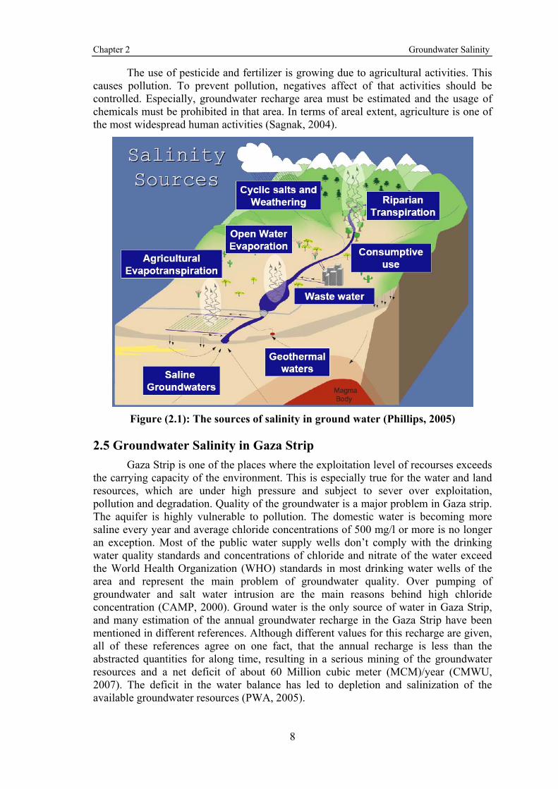
aquifer (CAMP, 2000). The sources of groundwater salinity can be divided into two naturally occurring pollutants and pollutants produced by human activities. The sources of salinity in ground water are illustrated in Figure (2.1).
2.4.1 Naturally Occurring Groundwater Pollution
2.4.1.1 Sea Water Intrusion
In the coastal plain where surface water is not enough and groundwater is limited, increasing water demand for tourism sector in addition to irrigation and domestic water supply is threat for groundwater. Finally, if groundwater is overexploited, sea water moves to the aquifer and quality of groundwater starts to deteriorate. Salt concentration increases (Sagnak, 2004).
2.4.1.2 Geothermal Affects
The chemical composition of groundwater is determined by composition of the materials it contacts and its duration. The longer contact period, the more minerals are dissolved. Especially, thermal water causes bad effects for fresh groundwater. It carries more minerals and materials deteriorating water quality. In addition this, during geothermal activities mineral water infiltrates. This is a big thread for unconfined aquifers (Sagnak, 2004).
2.4.1.3 Pollutants Originated From Geological Formation
Geological formation containing salt, gypsum, etc. In some groundwater basin, there are impervious barriers between fresh water bearing formations and salty water layers. When wrong drilling methods are used in these formations, salty water and fresh groundwater can be mixed and quality of fresh water can be deteriorated. A balance was established by the nature. But, in parallel to developing drilling activities, the balance has been affected due to wrong well construction. In order to prevent this, water movement among different aquifer systems should be studied and restricted.
2.4.2 Groundwater Pollution Produced by Human Activities
Pollution sources produced by human activities can be grouped into three general categories. These are municipal, industrial and agricultural disposal.
2.4.2.1 Municipal Disposal
Pollution sources may be point sources or non-point sources. In developing country, point sources are mainly municipal disposal due to fewer services such as poor sewerage systems. Rapid and uncontrolled urbanization over the areas that have groundwater potential is an important risk. In some areas, this may be more dangerous because of cracks, fractures and the high capacity of permeability. Also, the volume of municipal disposal is increasing day by day.
2.4.2.2 Industrial Disposal
Because many factories have been constructed on the aquifer systems and unfiltered waste water has been infiltrated to groundwater, heavy metal is analyzed in the groundwater. In order to minimize water pollution, waste water treatment plants have to be constructed. Besides, waste water should be stored in the waste water dam. So, seepage to the aquifer should be prevented or after treatment polluted water can be conveyed to disposal area.
2.4.2.3 Agricultural Pollutants
Chapter 2 Groundwater Salinity
8
The use of pesticide and fertilizer is growing due to agricultural activities. This causes pollution. To prevent pollution, negatives affect of that activities should be controlled. Especially, groundwater recharge area must be estimated and the usage of chemicals must be prohibited in that area. In terms of areal extent, agriculture is one of the most widespread human activities (Sagnak, 2004).
Figure (2.1): The sources of salinity in ground water (Phillips, 2005)
2.5 Groundwater Salinity in Gaza Strip
Gaza Strip is one of the places where the exploitation level of recourses exceeds the carrying capacity of the environment. This is especially true for the water and land resources, which are under high pressure and subject to sever over exploitation, pollution and degradation. Quality of the groundwater is a major problem in Gaza strip. The aquifer is highly vulnerable to pollution. The domestic water is becoming more saline every year and average chloride concentrations of 500 mg/l or more is no longer an exception. Most of the public water supply wells don’t comply with the drinking water quality standards and concentrations of chloride and nitrate of the water exceed the World Health Organization (WHO) standards in most drinking water wells of the area and represent the main problem of groundwater quality. Over pumping of groundwater and salt water intrusion are the main reasons behind high chloride concentration (CAMP, 2000). Ground water is the only source of water in Gaza Strip, and many estimation of the annual groundwater recharge in the Gaza Strip have been mentioned in different references. Although different values for this recharge are given, all of these references agree on one fact, that the annual recharge is less than the abstracted quantities for along time, resulting in a serious mining of the groundwater resources and a net deficit of about 60 Million cubic meter (MCM)/year (CMWU, 2007). The deficit in the water balance has led to depletion and salinization of the available groundwater resources (PWA, 2005).
Chapter 2 Groundwater Salinity
9
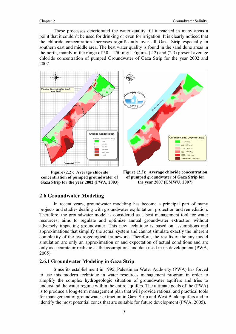
These processes deteriorated the water quality till it reached in many areas a point that it couldn’t be used for drinking or even for irrigation It is clearly noticed that the chloride concentration increases significantly over all Gaza Strip especially in southern east and middle area. The best water quality is found in the sand dune areas in the north, mainly in the range of 50 – 250 mg/l. Figures (2.2) and (2.3) present average chloride concentration of pumped Groundwater of Gaza Strip for the year 2002 and 2007.
Figure (2.2): Average chloride concentration of pumped groundwater of Gaza Strip for the year 2002 (PWA, 2003)
Figure (2.3): Average chloride concentration of pumped groundwater of Gaza Strip for
the year 2007 (CMWU, 2007)
2.6 Groundwater Modeling
In recent years, groundwater modeling has become a principal part of many projects and studies dealing with groundwater exploitation, protection and remediation. Therefore, the groundwater model is considered as a best management tool for water resources; aims to regulate and optimize annual groundwater extraction without adversely impacting groundwater. This new technique is based on assumptions and approximations that simplify the actual system and cannot simulate exactly the inherent complexity of the hydrogeological framework. Therefore, the results of the any model simulation are only an approximation or and expectation of actual conditions and are only as accurate or realistic as the assumptions and data used in its development (PWA, 2005).
2.6.1 Groundwater Modeling in Gaza Strip
Since its establishment in 1995, Palestinian Water Authority (PWA) has forced to use this modern technique in water resources management program in order to simplify the complex hydrogeologic situation of groundwater aquifers and tries to understand the water regime within the entire aquifers. The ultimate goals of the (PWA) is to produce a long-term management plan that will provide rational and practical tools for management of groundwater extraction in Gaza Strip and West Bank aquifers and to identify the most potential zones that are suitable for future development (PWA, 2005).

Chapter 2 Groundwater Salinity
10
In recognition the worsening situation of the water in Gaza Strip, PWA and United State Agency for International Development (USAID) have jointly developed the implementation of an Integrated Aquifer Management Plan (IAMP). The IAMP presented overall planning guidelines for water supply and usage through year 2020. As a result to this jointly, new model depending on Coupled Flow-Transport Modeling Code (DYNCFT) was conducted to simulate the effect of IAMP. DYNCFT is a model able to simulate 3-dimensional contaminant transport with dispersion and first-order decay and/or linear equilibrium adsorption. Conservative constituents (such as chloride and tritium) may be simulated as well. DYNCFT is based on the Lagrangian approach ('Random Walk" method for statistically significant number of particles, each particle having an associated weight, decay rate, and retardation). DYNCFT can also be used for transport modeling of dissolved contaminants, without variable density fluids. With the existing model PWA has an added capability to manage its resource, and equally importantly, to demonstrate what will happen if required investment are not made (Moe et al., 2001).
There are some researchers attempted to model the groundwater in Gaza Strip. Aish (2004) used GIS and MODFLOW in Artificial Recharge Modeling of the Gaza Coastal Aquifer. This research work investigates the first phase of a feasibility study on the impact of artificial recharge from a planned wastewater treatment plant on the groundwater quantity and quality of the coastal aquifer in the Gaza Strip. In the analysis of the results, the 100 mg/l of solute will be considered as the reference concentration (100% injected water) and the simulated concentration in the aquifer will be expressed relative to this value. The results indicate that 90% of the infiltrated water will be mixed with the aquifer water after 1 year beneath the recharge area with decreasing percentages in the surrounding area (Aish, 2004).
Ghabayen (2004) developed a model using Bayesian belief networks (BBNs), for Identification of salinity origin. The BBN model incorporates the theoretical background of salinity sources, area specific monitoring data that are characteristically incomplete in their coverage, expert judgment, and common sense reasoning to produce a geographic distribution for the most probable sources of salinization. The model showed areas where additional data on chemical and isotopic parameters are needed to understand the contribution of each of these sources to the problem. The model has successfully identified areas where seawater intrusion, deep brines, wastewater leakage, agricultural return flows, and Eocene waters exist with high probability. It has also identified areas where there is missing information or incomplete data especially in the eastern part of the coastal aquifer outside Gaza Strip (Ghabayen et al., 2004).
Qahman (2004) achieve a numerical assessment of seawater intrusion in Gaza Strip by applying a 3-D variable density groundwater flow model. A two-stage finite difference simulation algorithm was used in steady state and transient models. SEAWAT computer code was used for simulating the spatial and temporal evolution of hydraulic heads and solute concentrations of groundwater. A regular finite difference grid with a 400 m2 cell in the horizontal plane, in addition to a 12-layer model were chosen. The model has been calibrated under steady state and transient conditions. Simulation results indicate that the proposed schemes successfully simulate the intrusion mechanism. Two pumpage schemes were designed to use the calibrated model for prediction of future changes in water levels and solute concentrations in the groundwater for a planning period of 17 years. The results show that seawater intrusion would worsen in the aquifer if the current rates of groundwater pumpage continue. The alternative, to eliminate pumpage in the intruded area, to moderate pumpage rates from

Chapter 2 Groundwater Salinity
11
water supply wells far from the seashore and to increase the aquifer replenishment by encouraging the implementation of suitable solutions like artificial recharge, may limit significantly seawater intrusion and reduce the current rate of decline of the water levels (Qahman et al., 2004).
Barakat (2005) developed a model to find optimal values of water quantities from different resources in in the southern Gaza Strip. Visual Modflow (VMF) and its integrated modules, was developed to quantify, and analyze the raw input data. Many scenarios for domestic supply and demand reconfiguration are introduced. Genetic algorithm (GA) is used as a global optimization method, to find optimal values of water quantities from different resources. The resulted optimal values for water quantities were introduced into the groundwater model to predict water level contour maps in the next years (Barakat, 2005).
The use of ANN in groundwater quality modeling in Gaza Strip doesn’t found in large scale, Till now, only one researcher used it. Al Mahalawi used ANN in Modeling Groundwater Nitrate Concentration of the Gaza Strip (Mahalawi, 2007). My new research (Groundwater Salinity Modeling Using Artificial Neural Networks - Gaza Strip case study) might be considered as one of the few contributions in quantitatively modeling of the relation between groundwater salinity and the hydrological variables in spatial scale using ANN.

Chapter 3 Artificial Neural Networks
12
Chapter (3)
Literature Review/Artificial Neural Networks
3.1 Introduction to Artificial Neural Networks
ANN refer to computing systems whose central theme is borrowed from the analogy of biological neural networks. They represent highly simplified mathematical models of biological neural networks. They include the ability to learn and generalize from examples to produce meaningful solutions to problems even when input data contain errors or are incomplete, and to adapt solutions over time to compensate for changing circumstances and to process information rapidly (Jain et al., 2004).
The brain consists of a large number of neurons, connected with each other by synapses. These networks of neurons are called neural networks, or natural neural networks. ANN is a simplified mathematical model of a natural neural network. ANN are a new information-processing and computing technique inspired by biological neuron processing (Lee et al., 1998). The human brain provides proof of the existence of massive neural networks that can succeed at those cognitive, perceptual, and control tasks in which humans are successful. The brain is capable of computationally demanding perceptual acts (e.g. recognition of faces, speech) and control activities (e.g. body movements and body functions). The advantage of the brain is its effective use of massive parallelism, the highly parallel computing structure, and the imprecise information-processing capability. The human brain is a collection of more than 10 billion interconnected neurons. Each neuron is a cell that uses biochemical reactions to receive, process, and transmit information (Ajith, 2005). Figure (3.1) presented mammalian neuron.
Figure (3.1): Mammalian neuron (Ajith, 2005)
Treelike networks of nerve fibers called dendrites are connected to the cell body or soma, where the cell nucleus is located. Extending from the cell body is a single long fiber called the axon, which eventually branches into strands and sub strands, and are connected to other neurons through synaptic terminals or synapses. The transmission of signals from one neuron to another at synapses is a complex chemical process in which specific transmitter substances are released from the sending end of the junction. The effect is to raise or lower the electrical potential inside the body of the receiving cell. If

Chapter 3 Artificial Neural Networks
13
the potential reaches a threshold, a pulse is sent down the axon and the cell is ‘fired’ (Ajith, 2005).
Artificial neurons connected together form a network. The structure of ANN is, as rule, layered. Three functional group can be distinguished in the ANN ie the inputs receiving signals from the network’s outside and introducing them into its inside, the neuron which process information and the neurons which generate results. A model of the artificial neuron is shown in the Figure (3.2). The model include N inputs, one output, a summation block and an activation block (Hola and Schabowicz, 2005).
Figure (3.2): Model of artificial neurons (Hola and Schabowicz, 2005)
ANN is an informational system simulating the ability of a biological neural network by interconnecting many simple artificial neurons . The neuron accepts inputs from a single or multiple sources and produces outputs by simple calculations, processing with a predetermined non-linear function (Jeng et al., 2003).
The network topology consists of a set of nodes (neurons) connected by links and usually organized in a number of layers. Each node in a layer receives and processes weighted input from a previous layer and transmits its output to nodes in the following layer through links. Each link is assigned a weight, which is a numerical estimate of the connection strength. The weighted summation of inputs to a node is converted to an output according to a transfer function .
Most ANN has three layers or more: an input layer, which is used to present data to the network; an output layer, which is used to produce an appropriate response to the given input; and one or more intermediate layers, which are used to act as a collection of feature detectors. Determination of appropriate network architecture is one of the most important, but also one of the most difficult, tasks in the model-building process. Unless carefully designed an ANN model can lead to over parameterization, resulting in an unnecessarily large network (Sudheer et al., 2002). Figure (3.3) demonstrated schematic description of a general ANN model of three layers.

Chapter 3 Artificial Neural Networks
14
Figure (3.3): Schematic description of a three layer ANN and of the elements of its (mathematical) neurons (Claudius et al., 2005)
3.2 History of Artificial Neural Networks
A first wave of interest in ANN emerged after the introduction of simplied neurons by McCulloch and Pitts in 1943. These neurons were presented as models of biological neurons and as conceptual components for circuits that could perform computational tasks (Krose et al., 1996).
Hebb's book, 1949 presented the physiological learning rule for synaptic modification for the first time. Hebb proposes that the connectivity of the brain is continually changing as an organism learns differing functional tasks, and that neural assemblies are created by such changes. Rosenblatt 1958 introduced Perceptron which is novel method of supervised learning using perceptron convergence theorem. When Minsky and Papert published their book Perceptrons in 1969 (Minsky & Papert, 1969) in which they showed the deficiencies of perceptron models, most neural network funding was redirected and researchers left the field. Only a few researchers continued their efforts, most notably Teuvo Kohonen, Stephen Grossberg, James Anderson, and Kunihiko Fukushima (Krose et al., 1996).
The interest in neural networks re-emerged only after some important theoretical results were attained in the early eighties (most notably the discovery of error back-propagation), and new hardware developments increased the processing capacities. This renewed interest is reflected in the number of scientists, the amounts of funding, the number of large conferences, and the number of journals associated with neural networks (Krose et al., 1996).
Hopfield, 1982 showed how to use store information in dynamically stable networks. His work paved the way for physicists to enter neural modeling , thereby transforming the field of neural networks. Rumelhart, Hinton, and Williams 1986 developed the back-propagation algorithm, the most popular learning algorithm for the training of multilayer perceptrons. It has been the workhorse for many neural network

Chapter 3 Artificial Neural Networks
15
applications at that time. Since the late 1980s, ANN has been used successfully to model a variety of different functions. The network is able to learn these functions intelligently through an automatic training process (Lee et al., 1998).
Over the past decade, ANN has become increasingly popular in many disciplines as a problem solving tool. ANN have the ability to solve extremely complex problems with highly non-linear relationships. ANN’s flexible structure is capable of approximating almost any input-output relationships. Particularly ANN have been extensively used as a predicting and forecasting tool in many disciplines (Rajanayaka et al. , 2001). Nowadays most universities have a ANN group, within their psychology, physics, computer science, or biology departments (Krose et al., 1996).
3.3 Architectures of Artificial Neural Network
There are many ANN architectures, this property give ANN ability to solve a deferent models of data.
3.3.1 Simple Neuron (a single scalar input)
The central idea of ANN is that such parameters (weight, w & bias, b) can be adjusted in each training iterations. The neuron may be with or without bias.
3.3.1.1 Neuron Without Bias
The scalar input p is transmitted through a connection that multiplies its strength by the scalar weight w, to form the product wp, again a scalar. f is a transfer function (typically a step function or a sigmoid function). A neuron without bias is shown in Figure (3.4).
Figure (3.4): Neuron without bias (Matlab, 1994)
3.3.1.2 Neuron With Bias
This neuron has a scalar bias, b (is not an input) as simply being added to the product wp. A neuron with bias is shown in Figure (3.5).

Chapter 3 Artificial Neural Networks
16
Figure (3.5): Neuron with bias (Matlab, 1994)
3.3.2 Neuron With Vector Input
A neuron with a single R-element input vector is shown in Figure (3.6).
Figure (3.6): Neuron with Vector Input (Matlab, 1994)
Here the individual element inputs
P1,P2,…PR
Are multiplied by weights w1,1 ,w1,2 ,…w1,R
Their sum is simply Wp, the dot product of the (single row) matrix W and the vector p.
The neuron has a bias b, which is summed with the weighted inputs to form the net input , n . n = w1,1 P1 + w1,2 P2 + ... + w1,R PR + b
3.3.3 Layers of Neurons
3.3.3.1 Perceptron Network
A one-layer network with R input elements and S neurons called perceptron network. In this network, each element of the input vector p is connected to each neuron input through the weight matrix W. A layer is not constrained to have the number of its inputs equal to the number of its neurons. The neuron layer outputs form a column vector a.

Chapter 3 Artificial Neural Networks
17
The need is to make a distinction between weight matrices that are connected to inputs and weight matrices that are connected between layers. Weight matrices connected to inputs are called input weights. Weight matrices coming from layer outputs are called layer weights. Perceptron Network is shown in Figure (3.7).
Figure (3.7): Perceptron network (Matlab, 1994)
3.3.3.2 Multiple Layers of Neurons
A network can have several layers. Each layer has a weight matrix W, a bias vector b, and an output vector a. the three-layer network shown in Figure (3.8). The layers of a multilayer network play different roles. A layer that produces the network output is called an output layer. All other layers are called hidden layers. The three-layer network shown in Figure (3.8) has one output layer (layer 3) and two hidden layers (layer 1 and layer 2).
Figure (3.8): Multiple Layers of Neurons (Matlab, 1994)

Chapter 3 Artificial Neural Networks
18
3.4 Artificial Neural Networks Learning
There are several types of ANN learning. Supervised and unsupervised learning probably being the most important. In general, an ANN learns or is trained by adjusting the connection weights parameters, that link the neurons.
For classification and regression tasks supervised learning is used , where the available data set consists of corresponding input and output values representing a characteristic pattern or underlying functional behaviour. This data set is the so-called training set. The adaptation of the weights is carried out by an optimization algorithm that tries to minimize a difference or error measure between the ANN output based on the training set input values and their corresponding training set output value(s) (Govindaraju et al., 2000).
In unsupervised learning, the training of the network is entirely data-driven and no target results for the input data vectors are provided. ANN of the unsupervised learning type, such as the self-organizing map, can be used for clustering the input data and find features inherent to the problem. Unsupervised learning allegedly involves no target values. In fact, for most varieties of unsupervised learning, the targets are the same as the inputs (Sarle, 1994). In other words, unsupervised learning usually performs the same task as an auto-associative network, compressing the information from the inputs (Deco and Obradovic, 1996).
3.5 Types of Artificial Neural Networks
When Neural networks are trained, a particular input leads to a specific target output. Such a situation is shown Figure (3.9) There, the network is adjusted, based on a comparison of the output and the target, until the network output matches the target. Typically many such input/target pairs are used, in this supervised learning, to train a network.
Figure (3.9): Neural Network Mechanism (Matlab, 1994)

Chapter 3 Artificial Neural Networks
19
The network adopts as follows, change the weight by an amount proportional to the difference between the desired output and the actual output. As an equation
Delta Wi = L * (D-Y).Ii
Where L is the learning rate, D is the desired output, and Y is the actual output.
This is called the Perceptron Learning Rule, and goes back to the early 1960's. Back-Propagation (BP) witch sometimes known as multi-layer perceptrons (MLP) and Radial Basis Function Networks (RBF) are both well-known developments of the Delta rule for single layer networks that is a development of the Perceptron Learning Rule. There are many other methods of training as the Generalized Regression Neural Networks (GRNN) and Hopfield Networks. In this study only (MLP) and (RBF) were used in modeling process.
3.5.1 The Back Propagation (BP) Method
Back Propagation (BP) witch sometimes known as multi-layer perceptrons (MLP) distinguishes itself by the presence of one or more hidden layers, whose computation nodes are correspondingly called hidden neurons of hidden units. The function of hidden neurons is to intervene between the external input and the network output in some useful manner. By adding one or more hidden layers, the network is able to extract higher order statistics. In a rather loose sense, the network acquires a global perspective despite its local connectivity due to the extra set of synaptic connections and the extra dimension of the network interconnections (Haykin, 1994).
The ability of hidden neurons to extract higher order statistics is particularly valuable when the size of the input layer is large. The source nodes in the input layer of the network supply respective elements of the activation pattern (input vector), which constitute the input signals applied to the neurons (computation nodes) in the second layer (i.e., the first hidden layer). The output signals of the second layer are used as inputs to the third layer, and so on for the rest of the network. Typically, the neurons in each layer of the network have as their inputs the output signals of the preceding layer only. The set of the output signals of the neurons in the output layer of the network constitutes the overall response of the network to the activation patterns applied by the source nodes in the input (first) layer. (BP) are trained using the Levenberg–Marquardt optimization technique. Throughout all (BP) simulations, the learning rate and the momentum rate parameters were taken adaptively (Cigizoglu et al. , 2007). Generally the Figure (3.8) show the Architectures of back propagation method.
Training BP Networks
The weight change rule is a development of the perceptron learning rule. Weights are changed by an amount proportional to the error at that unit times the output of the unit feeding into the weight. Running the network consists of
1- Forward pass:
The outputs are calculated and the error at the output units calculated.
2- Backward pass:
The output unit error is used to alter weights on the output units. Then the error at the hidden nodes is calculated (by back-propagating the error at the output units through the weights), and the weights on the hidden nodes altered using these values.

Chapter 3 Artificial Neural Networks
20
For each data pair to be learned a forward pass and backwards pass is performed. This is repeated over and over again until a given number of epochs elapse, or when the error reaches an acceptable level, or when the error stops improving (you can select which of these stopping conditions to use).
3.5.2 The Radial Basis Function-Based Neural Networks (RBF)
RBF were introduced into the neural network by Broomhead and Lowe in 1988. The RBF consists of two layers whose output nodes form a linear combination of the basis functions. The basis functions in the hidden layer produce a significant non-zero response to input stimulus only when the input falls within a small localized region of the input space. Hence, this paradigm is also known as a localized receptive field network.
Transformation of the inputs is essential for fighting the curse of dimensionality in empirical modeling. The type of input transformation of the RBF is the local nonlinear projection using a radial fixed shape basis function. After nonlinearly squashing the multi-dimensional inputs without considering the output space, the radial basis functions play a role as regressors. Since the output layer implements a linear regressor the only adjustable parameters are the weights of this regressor. These parameters can therefore be determined using the linear least square method, which gives an important advantage for convergence (Cigizoglu et al. , 2007).
Radial basis networks consist of two layers: a hidden radial basis layer of S1
neurons, and an output linear layer of S2 neurons as shown in Figure (3.10).
Figure (3.10): Radial Basis function Networks (Matlab, 1994)

Chapter 3 Artificial Neural Networks
21
3.6 Building Artificial Neural Networks One of the critical issues in training the ANN model is to select input variables
that are highly correlated with studied problem. The choice of variables (at least initially) is guided by intuition. Understanding and expertise in the problem domain and conditions gives initially idea of which input variables are likely to be influential. Once in ANN, variables can be selected and deselect, and ANN can also determine useful variables (Jiang and Cotton, 2004).
After selecting variables, the following procedure must be achieved to build any Artificial neural networks
Determine the network properties:
The network topology (connectivity), the types of connections, the order of connections, and weight range.
Determine the node properties:
The activation range and the activation (transfer) function.
Determine the system dynamics:
The weight initialization scheme, the activation-calculating formula, and the learning rule.
Determine the topology of a neural network:
The topology of a neural network refers to its framework as well as its interconnection scheme. The number of layers and the number of neuron (or nodes) per layer often specify the framework. The types of layers include in the network are:
1- The input layer:
The nodes in it are called input units, which encode the instance data presented to the network for processing. For example, each input unit may be designated by an attribute value possessed by the instance.
2- The hidden layer:
The nodes in it are called hidden units, which are not directly observable and hence hidden , They provide nonlinearities for the network.
3- The output layer:
The nodes in it are called output units, which encode possible concepts (or values) to be assigned to the instance under consideration. For example, each output unit represents a class of objects.
A random sample of neural network that contain of three layers: an input layer of 4 neurons, one hidden layer of 7 neurons and an output layer of 1 neuron, as shown in Figure (3.11).

Chapter 3 Artificial Neural Networks
22
Figure (3.11): Random sample of neural network
In most situations, there is no way to determine the best number of hidden units without training several networks and estimating the generalization error of each. If you have too few hidden units, you will get high training error and high generalization error due to underfitting and high statistical bias. If you have too many hidden units, you may get low training error but still have high generalization error due to overfitting and high variance. So the best number of hidden layers depends in a complex way on:
The numbers of input and output units. The number of training cases. The amount of noise in the targets. The complexity of the function or classification to be learned. The architecture of neural network The type of hidden unit activation function. The training algorithm.
3.7 Artificial Neural Networks applications in Hydrology Over the past decade, ANN has become increasingly popular in many
disciplines as a problem solving tool. ANN has the ability to solve extremely complex problems with highly non-linear relationships. ANN’s flexible structure is capable of approximating almost any input-output relationships. Particularly ANN have been extensively used as a predicting and forecasting tool in many disciplines (Rajanayaka et al., 2001). Hydrologists are often confronted with problems of prediction and estimation of runoff, precipitation, contaminant concentrations, water stages, and so on most hydrologic processes exhibit a high degree of temporal and spatial variability and are further plagued by issues of nonlinearity of physical processes, conflicting spatial and temporal scales, and uncertainty in parameter estimates.
p1
p2
p3
p4
T
The input layer
The output
The hidden layer
P1 P2 P3 P4 Input data

Chapter 3 Artificial Neural Networks
23
Our understanding in many areas is far from perfect, so that empiricism plays an important role in modeling studies. Hydrologists attempt to provide rational answers to problems that arise in design and management of water resources. An attractive feature of ANN is their ability to extract the relation between the inputs and outputs of a process, without the physics being explicitly provided to them. They are able to provide a mapping from one multivariate space to another, given a set of data representing that mapping. Even if the data is noisy and contaminated with errors, ANN has been known to identify the underlying rule. These properties suggest that ANN may be well-suited to the problems of estimation and prediction in hydrology (Govindaraju et al., 2000).
Applications of ANN to hydrology are rapidly gaining popularity due to their power and potential in mapping nonlinear system data The neural network technology has provided many promising results in the field of hydrology and water resources simulation. In recent years, ANN has found a number of applications in the area of water quality modeling (Govindaraju et al., 2000). Applications of ANN to hydrology are rapidly gaining popularity due to their power and potential in mapping nonlinear system data (Jain et al., 2004).
In recent years, ANN has provided many promising results in the field of hydrology. ANN was used in many hydrologic applications as rainfall forecasting (Hung et al., 2008), rainfall-runoff relationship (Junsawang et al., 2007), Evaporation modeling ( Sudheer et al., 2002), and improving air temperature prediction (Smith et al., 2005).
The artificial neural network ANN, would seem to be a useful for modeling the most of water resources issues. The ANN are efficiency applicated in river flow prediction, in the rainfall-runoff relationship, in rainfall estimation, in various groundwater problems and many other applications (Cigizoglu, 2000) ANN also was applied in groundwater problems as simulating pumping index for hydraulic conductivity realization to remediate groundwater under uncertainty, modeling water table depth fluctuations (Rajanayaka et al., 2001) and estimation soil moisture (Jiang et al., 2004).
3.8 Artificial Neural Networks applications in Groundwater Quality Modeling
It is difficult to separate groundwater quality modeling and other hydrology modeling as different sections. Many articles have addressed both these topics to some extent. In recent years, ANN has found a number of applications in the area of water quality modeling. Water quality is influenced by many factors such as flow rate, contaminant load, medium of transport, water levels, initial conditions and other site-specific parameters. The estimation of such variables is often a complex and nonlinear problem, making it suitable for ANN application. There are several instances where ANN has been used to address groundwater quality related issues. For instance,
Sandhu and Finch (1996) used ANN to relate flow conditions and gate positions in the Sacramento San Joaquin Delta to salinity levels in the interior and along the boundary of the delta. ANN were further used to estimate flow in the Sacramento River to meet salinity standards. Sandhu and Finch (1996) found simulation models too slow and the commonly used statistical models to be inadequate, and they concluded that neural networks would be suitable for this application. Historical flows from various gauging stations and gate positions served as inputs to the network. Total dissolved

Chapter 3 Artificial Neural Networks
24
solids concentrations data for 20 years were available as network output. In their preliminary work, the authors used the data from 1980–1990 for calibration, and the data from 1971–1980 for validation. Future plans include more rigorous testing of neural networks for salinity predictions (Sandhu and Finch, 1996).
Rogers and Dowla (1992) employed an ANN, which was trained by a solute transport model, to perform optimization studies in ground-water remediation. They investigated hypothetical scenarios of one or several contaminant plumes moving through a groundwater region with a number of pumping wells. The wells could be on or off. The goal of remediation was to keep contamination concentration in some specified monitoring wells lower than the regulatory limit. The optimization arises in trying to minimize the total volume of pumping. A multilayer feed forward ANN was trained using the back-propagation training algorithm (Rogers and Dowla, 1994).
Morshed and Kaluarachchi (1998) used an ANN to estimate the saturated hydraulic conductivity and the grain size distribution parameter for application in the problem of free product recovery. They also concluded that the search process in the parameter space could be accelerated when the ANN was guided by a genetic algorithm (Morshed and Kaluarachchi, 1998).
Ray and Klindworth (1996) lay a blueprint for addressing the problem of agriculture chemical assessment in the rural private wells in Illinois using neural networks. They envisioned that important inputs would be depth to the aquifer material, well depth, land topography in the vicinity of the well, distance of potential contaminant sources from the well, and timing of precipitation with respect to pesticide application. They also discussed how data would be collected for such an application and commented about the utility of ANNs in such applications (Ray and Klindworth, 1996).
The use of ANN in groundwater quality modeling at Gaza Strip doesn’t found in large scale, Till now, only one researcher used it. Al Mahalawi used Artificial Neural Network in Modeling Groundwater Nitrate Concentration of the Gaza Strip (Mahalawi, 2007). This research - Groundwater Salinity Modeling Using Artificial Neural Networks Gaza Strip case study - might be considered as one of the few contributions in quantitatively modeling of the relation between groundwater salinity and the hydrological variables in spatial scale using ANN.

Chapter 4 Study Area Description
25
Chapter (4)
Study Area Description
4.1 Location and Population
The Gaza Strip is a narrow strip of land on the Mediterranean coast. It is situated in the southeastern coast of Palestine with longitudes of 34:21:38 E and Latitudes of 31:29:45 N. The area is bounded by the Mediterranean in the west, the 1948 cease-fire line in the north and east and by Egypt in the south The total area of the Gaza Strip is 365 km2 with approximately 40 km long and the width varies from 8 km in the north to 14 km in the south (UNEP, 2003). Figure (4.1) showed regional and location map of Gaza Strip.
In 1948, the Gaza Strip had a population of less than 100,000 people. By 2007, approximately 1.4 million Palestinians lived in the Gaza Strip, of whom almost one million were refugees. The current population is estimated to be in excess of 1.5 million, distributed across five Governorates. Gaza City, which is the biggest governorate, has about 400,000 inhabitants (UNEP, 2009). The estimated annual growth rate in Gaza Strip in 2007 is 3.8%. Table (4.1) presented the estimates of the population number and growth rate in Gaza Strip from 1997 to 2015 (PCBS, 2007).
Table (4.1) : The revised estimates of the population projection in Gaza Strip (PCBS, 2007)
Year Mid Year Population
Growth Rate (%)
Year Mid Year Population
Growth Rate (%)
1997 995,522 4.3 2007 1,499,369 3.8
1998 1,039,528 4.4 2008 1,556,201 3.7
1999 1,086,970 4.5 2009 1,614,018 3.6
2000 1,137,990 4.6 2010 1,672,785 3.5
2001 1,188,130 4.0 2011 1,732,438 3.5
2002 1,236,372 4.0 2012 1,792,895 3.4
2003 1,286,109 3.9 2013 1,854,353 3.3
2004 1,337,236 3.9 2014 1,917,019 3.3
2005 1,389,789 3.8 2015 1,980,825 3.2
2006 1,443,814 3.8
4.2 Topography
Gaza Strip is a coastal foreshore plain gradually sloping westward toward the sea allowing for surface run-off to rein filtrates the soil. A sandy beach stretches all along the coast, bound in the east by a ridge of sand dunes known as Kurkar ridges (Bruins et al., 1991).The altitude of the Gaza Strip land surface ranges between zero meters at the shore line to about 90 meters above mean sea level in some places, as shown in Figure (4.2).
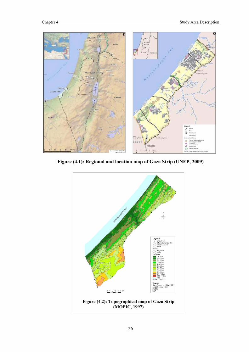
Chapter 4 Study Area Description
26
Figure (4.1): Regional and location map of Gaza Strip (UNEP, 2009)
Figure (4.2): Topographical map of Gaza Strip (MOPIC, 1997)

Chapter 4 Study Area Description
27
4.3 Climate and Rainfall
4.3.1 Climate
Gaza Strip area has a characteristically semi-arid mediterranean sea climate. It is located in transitional zone between a temperate mediterranean climate to the west and north, and the arid Negev and Sinai deserts to the east and south and there are two distinct seasons; cool and relatively wet season (October-March), and hot and dry season (April-September). The average daily temperature in the Gaza Strip ranges from 26°C in summer to 12°C in winter with the average daily maximum temperature range from 29°C to17°C ,and the minimum temperature range from 21°C to 9°C, in the summer and winter respectively. The daily relative humidity of this coastal area ranges from 65% to 85%in summer and from 60% to 80% in winter in the day time and at night respectively (GMS, 2005).
The wind velocity with northwest direction at 2 meter above the surface in the summer is about 1.5 m s-1 , which is less than that’s during winter months where velocity reaches values of 2.8 m s-1 (Haeyer, 2000).
The mean daily evaporation is variable during the year, where it ranges from about 2.1 mm/d, in December to 6.3 mm/d in July. The high potential evaporation is primarily related to high solar radiation incident over the strip at 190 kg-calories/cm2/year (U.S. National academy of Sciences, 1999). The generally cloudless summer months (April through September) and consequently open water evaporation is high in the summer, accounting for as much as 70 % of the annual total evaporation (GMS, 2005).
4.3.2 Rainfall
Rainfall is one of the most important parts of the water resource. It is an essential component of scientific investigation of the hydrologic cycle. The pattern, the amount beside the intensity of rainfall are the most important factors that directly affect to groundwater balance and replenishment in the Gaza Strip, rainfall is the main source of groundwater recharge area. The area is located in the semi-arid zone and there is no source of recharge other than rainfall therefore a detailed knowledge of rainfall regime and its distribution is a perquisite for water resources planning and management in Gaza Strip.
In Gaza Strip there are 12 manual rainfall stations distributed through different governorates as shown in Figure (4.3). Data from these stations are collected on a daily basis, these stations are operated by ministry of agriculture and data obtained from these stations are entered manually in Palestinian water authority database. The rainfall occurs in the winter period, which is between Octobers to March; and the mean annual rainfall varies 350-400 mm/year. The period for June to September is dry with no rainfall therefore the rainfall is the main source of almost all water in this area (GMS, 2005).
In the 2006-2007 season, average rainfall depth over Gaza Strip area is estimated about 364.7 mm with total amount 133.1 MCM received through 46 rainy days. Despite of the small area of Gaza Strip (365km2), the level of rainfall varies significantly from one area to the next with an average seasonal rainfall of 521.9 mm in north area (north governorate), to 225 mm in the southern area (Rafah Governorate) as shown in Figure (4.3) (PWA, 2007).

Chapter 4 Study Area Description
28
Figure (4.3): The rainfall depth in Gaza Strip
for 2006-2007 season (PWA, 2007) 4.4 Land Use
Land is one of the main scar natural resources in the Gaza Strip. Land is one of the primary natural resources in the Gaza Strip so land ownership is the major factors that play a role in any development plan. The major part of the Gaza Strip land is owned by the private sector. Figure (4.4) presented land use in Gaza Strip and Figure (4.5) presented the proposed future land use distribution in 2015.
The distribution of the proposed land use within the Gaza Strip per type of use for the year 2004 is illustrated in Table (4.2) derived from the study carried out by Ministry of Local Governorates (MOLG). Agriculture and assisting agriculture lands occupies about 47.5% of the land surface and the residential area represented 24%, public building 2.1%, where the main and secondary roads represented about 7.64% of the land surface.
Table (4.2): Proposed land use distribution in Gaza Strip in 2004 (MOLG, 2004)
Type of Use Area (km2) Area %
Main and Secondary Roads 27.875 7.64 % Public Building 7.675 2.10 % Residential Areas 87.745 24.04 % Industrial Area 12.445 3.41 % Gaza Airport 15.000 0.41 % Agricultural Area 167.675 45.94 % Assisting Agricultural Area 5.595 1.81 % Open and Green Areas 8.100 2.22 % Reserved Areas for Future Plans 25.450 6.97 % Others Area 19.940 5.46 % Total Area 365 100 %

Chapter 4 Study Area Description
29
#
#
#
#
#
#
#
#
Sea
Agricultural Land UseAlmondsCitrusCitrus/HorticultureDatesGrapesGreenhousesHorticultureOlivesRainfed Crops
Built-up areas
RoadsRegionalMain
WadiDelimiting LineInternational Border
# Entry Point
Scale 1:200,000
Sources:Cairo Agreement Map, 1994Aerial Photos, 1996MOPIC
Legend
0 1 2 3 4 5 km
N
MEDIT
ERRANEAN S
EA
Figure (4.4): Land use in Gaza Strip (MOPIC, 1998)
Figure (4.5): The proposed future land use distribution in 2015 (MWGP, 2001)

Chapter 4 Study Area Description
30
4.5 Geology
The Gaza Strip is a shore plain gradually sloping to the west. It is underlain by a series of geological formations from the Mesozoic to the Quaternary. The main formations known were composed in the last two system periods, Tertiary formation called “Saqiya formation” of about 1200-meter thickness, and the Quaternary deposits in the Gaza Strip are of about 160 meters thickness and cover Saqiya formation (Mortaja, 1998). Table (4.5) summarizes the geological history of the Gaza Strip, where Figure (4.6) illustrates a geological cross-section in the Gaza Strip.
Table (4.3): Geology and geological history of the Gaza Strip (Palestinian Environmental Protection Authority, 1994) and (Hamdan, 1999)
Era
Sys
tem
Per
iod
Ser
ies
Age
mil
lion
ye
ars
For
mat
ion
En
viro
nm
ent
of D
epos
itio
n
Lit
hol
ogy
Max
. T
hic
kn
ess
(m)
Wat
er B
eari
ng
Ch
arac
ter
Hol
ocen
e
0.01 Alluvial Terrestrial
Sand, loess, calcareous silt and gravel
25 Locally phreatic aquifer
Continental Kurkar
Aeolian Fluvial
100 Main aquifer
Qu
ater
nar
y
Ple
isto
cene
1.8 Marine Kurkar
Near Shore 100 Main aquifer
5 Conglome-rate
Near Shore Conglomerate
20
Base of the coastal Zone aquifer
Pli
ocen
e
12 Saqiya Shallow marine
Clay , Marl, Shale
1000
Aquiclude
Cen
ozoi
c
Ter
tiar
y
Neo
gen
e
Mio
cene
22.5 Marine
Marl, Limestone, Sandstone and Chalk
500
Aquiclude alternating permeable layers with saline water
Mesozoic
Paleozoic
Precambrian

Chapter 4 Study Area Description
31
Figure (4.6): A geological sross-section in the Gaza Strip. (Metcalf and Eddy, 2000)
The geological formations deposited in the area are described as follows:
4.5.1 Tertiary Formation
The tertiary formations are composed mainly of Saqiya formation, which consist of clay, Marl and Shale, and overlies the limestone layer beneath. (Hamdan, 1999).The thickness of this formation is about 1200 m at the shoreline, and it descends down rapidly at the east. According to oil exploitation logs, it is found that there are other Tertiary formations such as Chalks, limestone, and sandstonge at depths of 2000 m.
4.5.2 Quaternary Formation
The quaternary deposits have a thickness of about 160 m and covering the Pliocene Saqiya formation. Overlying Pleistocene deposits “Lower Quaternary “, consists of :
4.5.2.1 Marine Kurkar Formation
It is composed of shell fragments and quartz sands with calcareous cement. The thickness varies between 10 to 100 meters on the coast.
4.5.2.2 Continental Kurkar Formation
It is composed of red loamy sand beds (Hamra). The maximum thickness is about 100 meters with often-calcareous cement (PEPA, 1994).
4.5.2.3 Quaternary Deposits
These deposits are found at the top of the Pleistocene formation with a thickness up to 25 m. It can be divided into the following different types:
1. Sand Dunes
Sandy soil is found in the dunes area along the southern seashore, in a width of 2-3 km. The total area of the sandy covers about 70 km2. The sand dunes are 30-50 m above sea level. Lucite soil is widely spread in the middle of Gaza. This soil is a mixture of sand and loam (Palestinian Environmental protection Authority, 1994).

Chapter 4 Study Area Description
32
The thickness of these dunes is about 15 m. These dunes originate partly from Nile river sediments. It extends along the shoreline, with small width in the south, increasing northward up to 3 km.
2. Sand Loess and Gravel Beds.
It has a small thickness of about 10 m, and it is considered as the main formation of Wadi Gaza.
3. Alluvial Deposits.
These formations have a thickness of 25 m and spreading around the Wadi Gaza.
4. Beach Formation
It composed of relatively thin layer of sand with shell fragments. It is mainly unconsolidated, however; in some places, it is cemented due to deposition of calcium carbonate.
4.6 Soil Condition
4.6.1 Subsoil Formation
The deposits formed in the Pleistocene and Holocene ages are classified as subsoil formations and soil respectively. The subsoil formations from the Pleistocene age are distinguished in two categories that are:
4.6.1.1 Kurkar
Kurkar formations results from the continuous deposition of sand through the Pleistocene age in a sedimentary basin, which extends beyond the border of the coastal region. The sand was deposited as Aeolian dunes that consolidated later by litho static pressure and precipitation. Cemented sandstone are present near the surface, they form distinctive topographic ridges with vertical relief up to 60 meter. These Kurkar ridges, from which the coastal aquifer has obtained its name, typically extend in NE-SW direction. Hamdan (1999) emphasized that this formation is the water-bearing layer that allows significant amounts of water to go through. The hydraulic conductivity (the rate at which the formation allows water to go through) of Kurkar depends on the type of the cement (clay mineral, calcium carbonate) (Hamdan,1999).
4.6.1.2 Hamra
Hamra and Kurkar are found in consecutive stratification and formed in the Pleistocene and Holocene series of the Quaternary system. Hamra and Kurkar interchange each other on the outcrops at the ground surface of the Gaza Strip. Hamra formation is a mix of clay, silt and fine grains that are covered by iron oxides with red color. The formation is free of lime and founded in beds at different depths of about one meter thickness. Besides, it can be found in fragmented small layers.
4.6.2 Soil Formation
Soil is the surface layer that covers the rock formation; it is affected by the parent rock and the local climate. It contains a mixture of organic and inorganic constituents, water and air.
As shown in Figure (4.7) soils classification based on soil texture (MOPIC, 1997). Another classification considered the outward properties and soil physical properties in various depths (30 cm, 60 cm, 90 cm, 100 cm) (Goris and Samain, 2001).

Chapter 4 Study Area Description
33
The classification and the characteristics of different soil types of Gaza Strip are summarized in Table (4.4).
Soil.shpDark brown / Silty ClayLoess soilsLoessal sandy soilSandy loess soilSandy loess soil over loessSandy regosols
Figure (4.7): Soil Classifications in Gaza Strip (MOPIC, 1997)
Table (4.4): Classification & characteristics of different soil types in Gaza Strip. Adopted from (MOPIC, 1997; Goris and Samain, 2001)
Texture Description Location Local
Classification
Sandy loam (6% clay, silt 34% , sand 58%)
Loess soils sedimented in Pleistocene until Holocene Series. The grain size of loess fluctuates from 0.002 to 0.068 mm. Loess has been transported by winds and sedimented in loose form in the upper part, and in hard form in the lower part of the layers. They are brownish yellow-colored often with accumulation of lime concretions in the subsoil and containing 8 – 12 % calcium carbonate.
Between the Gaza city and the Wadi Gaza
Loess soil

Chapter 4 Study Area Description
34
Sandy clay loam (25% clay, 13% silt, 62% sand)
These alluvial soils are Usually dark brown to reddish in colour, with a well-developed structure. At some depth, lime concretions can be found. The calcium carbonate content can be around 15–20%
Beit Hanoun and Wadi Gaza
Dark brown /reddish brown
Sandy clay loam (23% clay, 21% silt, 56% sand)
This is a transitional soil, characterized by a rather uniform, lighter texture. Apparently, windblown sands have been mixed with loessial deposits.
Deir el Balah and Abssan
Sandy loess soil
The top layer is sandy loam (14% clay, 20% silt, 66% sand). The lower profile is loam (21% clay, 30% silt, 49% sand)
Forms a transitional zone between the sandy soil and the loess soil, usually with a calcareous loamy sandy texture and a deep uniform pale brown soil profile.
It is found in the central and southern part of the strip
Loessial sandy soil
Sandy loam (17.5% clay, 16.5% silt, 66% sand)
It is loess or loessial soils which have been covered by a 20 to 50 cm thick layer of sand dune
It is found east of Rafah and Khan Younis
Sandy loess soil over loess
Top layer is loamy sand (9% clay, 4% silt, 87% sand). Deeper profile is sand (7.5% clay, 0% silt, 92.5% sand)
Soil without a marked profile. Texture in the top meters is usually uniform and consists of medium to coarse quartz sand with a very low water holding capacity. The soils are moderately calcareous, very low matter and chemically poor, but physically suitable for intensive horticulture in greenhouses. In the deeper subsurface occasionally loam or clay loam layers of alluvial origin can be found
It is found a long the coast of Gaza Strip
Sandy regosol
4.7 Hydrology
Precipitation falling on land is either returned directly to the atmosphere by evaporation, flows along the land surface to become surface water or percolate into the round. Water that infiltrates into the ground is either drawn into plants and returned to the atmosphere by transpiration or continues infiltrating and becoming groundwater.
4.7.1 Surface Water Hydrology
The surface water system in the study area is Wadi Gaza. Wadi Gaza that located at the southern boundary of study area is the bigger in Gaza Strip. It runs in the central part of the Gaza Strip and discharge into the Mediterranean Sea Wadi Gaza length is about 9 km in Gaza and it extends into the armistice border for about 95 km where it collects the water from a big catchment area (3600 km2) from the Hebron Mountains and the Northern Negeve. This main stream was diverted by the Israelis to an adjacent area where it's been stopped their and collected at basins located 6km east of Gaza (MWCP, 2001).

Chapter 4 Study Area Description
35
Wadis are ephemeral streams, characterized by short duration floods that occur after heavy rainfall, while most of the time they are completely dry. Freshwater flows into them in the winter season. Israel has retained and changed the course of the two Wadis and they become dry since the early seventies, this means that fresh surface water resources are negligible.
4.7.2 Groundwater Hydrology
The coastal aquifer underlies the Coastal Plain of Palestine and runs parallel to the Mediterranean Sea coast. The coastal aquifer is an underground phreatic reservoir varies in width from 7 km in the north to 20 km in the south; its thickness decreases eastwards from 200 m near the coastline to a few meters in the eastern margins (PWA, 2000a). The aquifer (the Kurkar Group of Pleistocene age) consists of sand, sandstone, and silt interbedded with marine clays, and it overlies the impervious marine clays of upper Eocene to Pliocene age (the Saqiye Group). The aquifer is basically phreatic, but clay layers divide it vertically into several subaquifers. The hydraulic connection between groundwater in the different subaquifers and the sea is not well understood. While Bear and Kapuler (1981) considered that all subaquifers are connected to the sea, Kolton (1988) argued that the lower subaquifers are disconnected (Oren, et al., 2004). In the central and eastern areas the aquifer is uniform and phreatic. The calcareous sandstone (arenites or "kurkar") is composed of several minerals: quartz, feldspar, calcite, aragonite, and iron oxides (Vengosh, et al., 1996).
4.7.2.l Hydrostratigraphy
In the study area, the coastal plain aquifer contains many diverse hydraulic and hydrologic units and thus, several water-producing zones. The layered stratigraphy of the Kurkar Group subdivides the coastal aquifer from top to bottom into four separate sub-aquifers near the coast A, Bl, B2 and C as shown in Figure (4.6) . This subdivision is conditioned by impervious to semi-impervious interlayers alternating with predominantly permeable calcareous sandstones, and persists along the coastal strip but dissipates 4-6 km east of the shoreline. East of the third ridge the Kurkar Group sequence is randomly subdivided by occasional occurrence of impervious to semi-impervious layers and the coastal aquifer can be regarded as one hydrogeological unit. The upper subaquifer "A is unconfined, whereas subaquifers "Bl, B2, and C become increasingly confined towards the sea (Al-Jamal and Yaqubi, 2000).
4.7.2.1.l Kurkar Group
Sub-aquifer A:
Sub-aquifer (A) occurs in the uppermost and westernmost part of the sequence extends from the shoreline to the east up to 2 km. It is mainly composed of variously cemented concretionary calcareous sandstone mixed and interlayered with loose sand, of both continental and littoral origin. This aquifer is bounded from the top by the water table and at the bottom partly bounded by the first aquitard of silty clay. In the study area, it is 25m thick in the east to about 60-m in the west. This aquifer unit overlies continental-estuarine clay or loam extending eastwards and upwards, reaches in thickness to 15 m. However, the clay-rich base layer of sub-aquifer A is not always continuous and therefore, the hydrogeological and hydro stratigraphical separation between sub-aquifer A and underlying subaquifer B does not always exist or can be clearly identified. Sub-aquifer A may contain thin interlayers of clay, sandy clay and silty clay, which act as aquitards.

Chapter 4 Study Area Description
36
Sub-aquifer B1:
Based on Israel studies of Ecker, 1999 sub-aquifer B1 is mainly from Kurkar and micro-conglomerate deposited in a more littoral environment, the cementation of which is harder than in the overlying sub-aquifer A and having a lower proportion of loose sand. The base of this sub-aquifer is formed by marine to lagoonal-estuarine clays. Further eastwards, these base layers turn into continental clays and loarns and extend 6-7 km east of the shoreline.
Sub-aquifer B2
The calcareous sandstones of this unit are predominantly products of a high-energy littoral depositional environment, such as conglomerates and beach rock overlying a marine clay horizon. Based on Israel studies sub-aquifer B2 is 20-40-m thick. Near the coastline, sub-aquifer B2 occurs between elevations of (- 120) and (- 150) m below MSL (Zilberbrand et al., 2001).
Sub-aquifer C
Between the shoreline and 3-4 km inland, the lithology of this sub-aquifer is of a marine type, with no indications of shallower facies. It is characterized by interlayering of clay, silt, and silty sand, 10-20-m thick. Generally, the occurrence of calcareous sandstones increases eastwards on account of silty-clayey beds. The hydraulic conductivities of this unit are significantly lower than in the overlying sub-aquifers. Sub-aquifer C overlies impervious layers related to top of the Saqiye Group. Their occurrence is usually marked by thin streaks of chalky and marly sandstone, yellowish chalky marl, and clays. The top of the Saqiye occurs at elevations of -150 to -160 m below MSL, close to the shoreline (Zilberbrand et al., 2001).
4.7.2.1.2 The Saqiye Group
The Pleistocene Coastal Plain aquifer system (the Kurkar Group) overlies a very thick complex of shales and marls related to the Plio-Pleistocene Saqiye Group that wedges out gradually eastwards. In the study area its maximum depth reaches 1900 m near the coastline, wedging out in the eastern parts of the Coastal Plain. The top of the Saqiye Group dips 1-2% westwards (Zilberbrand et al., 2001).
4.7.3 Aquifer Hydraulic Properties
4.7.3.1 Transmissivity
From results of aquifer tests carried out in Gaza Strip, transmissivity values range between 700 and 5000 square meters per day (m2/d).corresponding values of hydraulic conductivity K are mostly within a range of 20-80 meters per day (m/d). Most of the wells that have been tested are municipal wells screened across more than one sub-aquifer. Hence, little is known about any differences in hydraulic properties between sub-aquifer (PWA, 2000b).
4.7.3.2 Effective Porosity:
Groundwater velocity is inversely proportional to effective porosity. Thus, a reduction in effective porosity implies in an increased velocity and hence faster migration of a particular contaminate. The base case calibration value is 25%.three sensitivity runs were carried out 15%, 20%, and 30% (PWA, 2000b).

Chapter 4 Study Area Description
37
4.7.3.3 Specific Yield and Specific Storativity
Specific yield values are estimated to be about 15-30 percent while specific storativity is about 10-4 from tests conducted in Gaza. Concerning the specific yield values is asking only about the porosity so the porosity values are consistent with the specific yield values (effective porosity 25%) for the sand and gravel (PWA, 2000b). Table (4.5) represented hydraulic properties in Gaza Strip subaquifers
Table (4.5): Aquifer hydraulic properties (PWA, 2000b)
Stratigraphic Unit
Horizontal Hydraulic
Conductivity (m/d)
Vertical Hydraulic
Conductivity (m/d)
Specific Yield
Specific Storativity'
(m-1)
Subaquifer A 30.0 3.00 0.25 0.1 E-04
Subaquifer B1 30.0 3.00 0.25 0.1 E-04
Subaquifer B2 30.0 3.00 0.25 0.lE-04
Subaquifer C 30.0 3.00 0.25 0.lE-04
Coastal Clays / Aquitards
0.20 0.20 0.10 0.lE-04
Undifferentiated Aquifer East of Coastal Clays
5.0 - 30.0 0.5 - 3.0 0.25 0.lE-04
4.7.4 Groundwater Balance
In order to analyze the water balance in the Gaza Strip, it is necessary to compare water supply with water demand (Assaf, 2001). It should be noted that, the Gaza coastal aquifer is a dynamic system with continuously change inflow and outflow. The present net aquifer balance is negative, that is a water deficit. Under defined average climate condition and total abstraction and return flows; the net deficit range between 18-26 Mm3/yr. as shown in Table (4.6).
In the year 2020, there will be 2 million inhabitants, double the current population, and the water demand could easily double from the current 170 Mm3/yr. to 216 Mm3/yr., which makes it necessary to generate and obtain additional water supplies in order to cover these alarming shortages (Adopted from Metcalf and Eddy, 2000).
Table (4.6): Estimated water balance of Gaza Strip (Adopted from Metcalf and Eddy, 2007)
Inflows (Mm3/yr.) Outflows (Mm3/yr.)
Min. Max. Min. Max.
Rainfall recharge 40.0 45.0 Municipal abstraction 80.0 85.0
Lateral inflow from Israel 18.0 30.0 Agriculture abstraction 80.0 100.0
Lateral inflow from Egypt 2.0 5.0 Mekorot abstraction 5.0 8.0

Chapter 4 Study Area Description
38
Saltwater intrusion 10.0 15.0 Discharge to the sea 10.0 15.0
Water system leaks 10.0 15.0
Wastewater return flow 10.5 10.5
Irrigation return flow 20.0 25.0
Loss of aquifer storage 2.0 3.0
Other recharge 3.5 3.5
Total 116 152 175 208
Net balance 59 56

Chapter 5 Methodology
39
Chapter (5)
Methodology
5.1 Introduction
This chapter discusses the utilized methodology in this research. Many techniques, approaches and tools were used to achieve the objectives of this research.
In order to model the groundwater salinity in Gaza strip using ANN it is necessary to gather data for training purposes. The training data must include a number of cases, each containing values for input and output variables. The first decisions needed are: which are variables to use, and how many (and which) cases to gather? The choice of variables (at least initially) is guided by intuition. Understanding and expertise in the problem domain and conditions give initially idea of which input variables are likely to be influential. Once in ANN, variables can be select and deselect, ANN can also experimentally determine useful variables. As a first pass, any variables which could have an influence on groundwater salinity should be included on initial studies.
Initially, it is assumed that the groundwater salinity (represented by chloride concentration mg/l) may be affected by some variables as: recharge rate (R), abstraction (Q), abstraction average rate (Qr), life time (Lt), groundwater level (Wl), aquifer thickness (Th), depth from surface to well screen (Dw), and distance from sea shore line (Ds). These variables were chosen depending on the literature review in Chapter two.
5.2 Data Collection and Preparation
The required data were extracted mainly from the domestic wells in Gaza Strip because it usually have quality test twice a year in February and October periodically. The quality test includes the chloride concentration test which gives us a great chance to monitor groundwater salinity in Gaza Strip and it's changes two times per year. The assumed variables will be gathered, studied, validated and rearranged to create training data matrix which should contain many hundreds of cases each containing values for input variables and output.
It is noted that the raw data available with institutions at Gaza Strip may have some errors which mainly associated with human error and many necessary data had been lost or not found. This confuse the work and restrict the ability to collect large quantity of data which have negative effect on the performance of the new constructed model.
In this research, it is necessary to deal with regular time series data to construct data training matrix so many sources of data have been neglected because of the deficiency of complete required data. Since that the detailed abstraction records have not been obtained for years prior to 1996, the period of model which include the modeling and calibration starts from 1997 to 2006. The methodology of gathering and preparation each variable is discussed in the following sections.
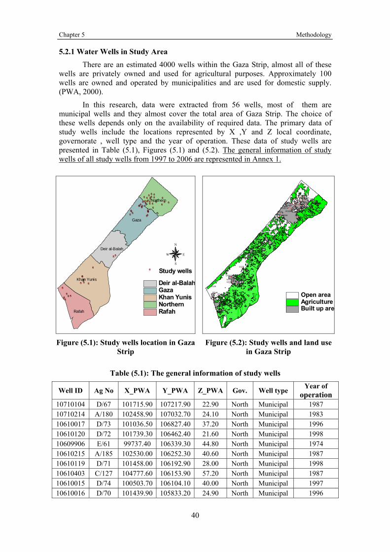
Chapter 5 Methodology
40
5.2.1 Water Wells in Study Area
There are an estimated 4000 wells within the Gaza Strip, almost all of these wells are privately owned and used for agricultural purposes. Approximately 100 wells are owned and operated by municipalities and are used for domestic supply. (PWA, 2000).
In this research, data were extracted from 56 wells, most of them are municipal wells and they almost cover the total area of Gaza Strip. The choice of these wells depends only on the availability of required data. The primary data of study wells include the locations represented by X ,Y and Z local coordinate, governorate , well type and the year of operation. These data of study wells are presented in Table (5.1), Figures (5.1) and (5.2). The general information of study wells of all study wells from 1997 to 2006 are represented in Annex 1.
#S #S#S #S #S#S#S#S #S #S#S #S#S #S#S#S #S#S#S #S#S#S
#S #S#S#S#S#S
#S#S
#S#S#S#S#S #S
#S
#S#S#S
#S
#S #S#S#S#S #S #S
#S#S #S
#S #S
#S
#S
#S
Gaza
Khan Yunis
Rafah
Northern
Deir al-Balah
Deir al-BalahGazaKhan YunisNorthernRafah
#S Study wells
N
EW
S
Figure (5.1): Study wells location in Gaza Strip
# #
# # ##
# # # ## ## ### ### #
##
# ####
#
##
#
#### #
#
##
##
###
## #
#
#
# #
##
#
#
#
E/4E/6
E/61
D/74D/60
E/90C/76
R/74
S/69
L/87L/43
L/41
P/15
C/79
Q/68
R/75
A/180 C/127
E/154
E/157
R/112 R/25A
R/254
J/146
L/159
L/127L/176
P/139
P/144
P/138
R/113
R/265
L/179
P/145
R/162B
R/162GR/162H
L/159A
R/162LA
Built up areAgricultureOpen area
Figure (5.2): Study wells and land use in Gaza Strip
Table (5.1): The general information of study wells
Well ID Ag No X_PWA Y_PWA Z_PWA Gov. Well type Year of
operation 10710104 D/67 101715.90 107217.90 22.90 North Municipal 1987 10710214 A/180 102458.90 107032.70 24.10 North Municipal 1983 10610017 D/73 101036.50 106827.40 37.20 North Municipal 1996 10610120 D/72 101739.30 106462.40 21.60 North Municipal 1998 10609906 E/61 99737.40 106339.30 44.80 North Municipal 1974 10610215 A/185 102530.00 106252.30 40.60 North Municipal 1987 10610119 D/71 101458.00 106192.90 28.00 North Municipal 1998 10610403 C/127 104777.60 106153.90 57.20 North Municipal 1987 10610015 D/74 100503.70 106104.10 40.00 North Municipal 1997 10610016 D/70 101439.90 105833.20 24.90 North Municipal 1996

Chapter 5 Methodology
41
5.2.2 Chloride Concentration Data
Groundwater quality in Gaza Strip is monitored by different institutions as Ministry of Health (MOH) and Ministry of Agriculture (MOA). This research concerns with data of MOH because it usually performs quality test twice a year in February and October periodically. MOA do not adhere periodically tests, and so it is impossible to make periodical monitor of chloride concentration and salinity using agriculture wells.
The data of some domestic wells were neglected because of the lost of some necessary required data especially in chloride concentration and abstraction data. Table 5.2 presents chloride concentration of some study wells from 1997 to 2000. Figure (5.3) presented average chloride concentration of pumped Groundwater of Gaza Strip for the year 2007. The chloride concentration of all study wells from 1997 to 2006 are represented in Annex 2.
Table (5.2): Chloride concentration (mg/l) of some study wells from 1997 to 2000
Ag No 01/0
4/19
97
01/1
0/19
97
01/0
4/19
98
01/1
0/19
98
01/0
4/19
99
01/1
0/19
99
01/0
4/20
00
01/1
0/20
00
D/67 78.0 55.0 56.0 56.0 42.0 NA 42.0 35.3 A/180 35.0 NA 49.0 56.0 49.0 63.0 70.0 77.0 D/73 NA NA 56.0 63.0 63.0 63.0 63.0 56.0 D/72 NA NA NA 71.0 77.0 NA 70.0 63.0 E/61 66.0 145.0 42.0 135.0 182.0 NA 385.0 749.0
A/185 70.0 100.0 77.0 85.0 84.0 77.0 91.3 91.0 D/71 NA NA 70.0 78.0 74.0 66.0 77.0 70.0 C/127 92.0 100.0 70.0 70.0 77.0 84.0 77.0 77.0 D/74 56.0 65.0 56.0 71.0 77.0 77.0 77.0 77.0 D/70 79.0 NA 70.0 85.0 88.0 NA 91.0 91.0
Figure (5.3): Average chloride concentration of pumped groundwater of
Gaza Strip for the year 2007 (CMWU, 2007)

Chapter 5 Methodology
42
5.2.3 Recharge Rate
Recharge refers to the entrance of water into soil or porous material through the interstices or pores of a soil or other porous medium. Infiltration is the sole source of soil water to sustain the growth of vegetation and of the groundwater supply of wells, springs, and streams (Schwab et al., 1993).
The capacity of any soil to absorb the rainwater falling continuously at an excessive rate goes on decreasing with time until a minimum rate of infiltration reached. The infiltration rate is a function of time, and has the dimensions of volume per unit of time per unit of area. These units reduce to depth per unit time; it is expressed in (mm/min) (Suresh, 1993).
Major component of recharge in the Gaza coastal aquifer model include :
Recharge from rainfall.
Return flows from irrigation.
Return flow from other sources (water distribution systems, septic systems, and wastewater collection systems, wadi Gaza and infiltration basins) (CAMP, 2000).
5.2.3.1 Factors Influence Infiltration Rate.
The infiltration rate differs from one type of soil to another However, since the increasing urban development, the natural soil was disturbed and covered by impermeable layers such as paved roads or occupied by buildings. This, of course reduced drastically the amount of infiltrated rainfall that replenishes the groundwater. The decrease in infiltrated rainwater appeared as a surface run-off, is lost by either evaporation or diverted to the sea.
The infiltrated water in Gaza Strip goes through the soil in a rate of one to two meters per day in the areas where fine sand is found, and this rate increases in the coarser formation e.g. kurkar. However, the percolation rate decreases, if it encounters a clayey layer in the subsurface. Water goes horizontally above the non-permeable layer until it encounters a disconnection in this layer and travels vertically downward to groundwater reservoir (PWA, 2003).
The National Soil Survey Center in cooperation with (NRCS) and the U.S Agricultural Research Service (USDA) suggested in (1998) that a number of factors, which affect soil infiltration, some of these factors, are follow:
1- Crust
Soils that have many large surface connected pores have higher intake rates than soils that have few such pores. A crust on the soil surface can seal the pores and restrict the entry of water into the soil.
2- Compaction
A compacted zone or an impervious layer close to the surface restricts the entry of water into the soil and tends to result in pounding on the surface.
3- Soil Texture
The type of soil (sandy, silty, and clayey) can control the rate of infiltration. For example, a sandy surface soil normally has a higher infiltration rate than a clayey

Chapter 5 Methodology
43
surface soil. Hamdan (1999) suggested that soil texture is important to identify the vulnerability of the artificial recharge basin to surface sealing, where a thin lamina of fine particles covers the surface of spread basin will decrease the infiltration much more clogging. Goris and Samain (2001) described the texture of five different soils in Gaza strip, while Hamdan (1999) added another sixth one as shown in table (5.3).
Table (5.3): Texture and infiltration Parameters of the Different Soil Types in the Gaza Strip (Goris and Samain, 2001) and (Hamdan, 1999)
Soil type Clay %
Silt%
Sand %
Soil texture
Initial infiltration rate
(f o ) mm/hr
Basic infiltration
rate ( f b )mm/hr
soil parameter
( k )
Sandy regosol 08.5 01.8 89.8 Sandy 1263.0 401.4 0.24 Sandy loess soil over loess
17.5 16.3 66.2 Sandy loam
357.6 97.2 0.08
Loessial sandy soil
18.0 25.0 57.0 Sandy loam
498.6 145.8 0.08
Dark brown/ reddish brown
25.3 12.8 61.9 Sandy clay loam
1051.2 208.8 0.11
Sandy loess soil
23.2 20.3 56.5 Sandy clay loam
270.6 66.0 0.06
Loess soil 06.0 34.0 58.0 sandy loam
428.1 121.5 0.08
# #
# # ##
# # # ## ## ### ### #
##
# ####
#
##
#
#### #
#
##
##
###
## #
#
#
# #
##
#
#
#
E/4E/6
E/61
D/74D/60
E/90C/76
R/74
S/69
L/87L/43
L/41
P/15
C/79
Q/68
R/75
A/180 C/127
E/154
E/157
R/112 R/25A
R/254
J/146
L/159
L/127L/176
P/139
P/144
P/138
R/113
R/265
L/179
P/145
R/162B
R/162GR/162H
L/159A
R/162LA
Dark brown / Silty ClayLoess soilsLoessal sandy soilSandy loess soilSandy loess soil over loessSandy regosols
N
EW
S
Figure (5.4): The study wells according to soil types of Gaza Strip

Chapter 5 Methodology
44
4- Organic Matter An increased amount of plant material, dead or alive, generally assists the process of infiltration. Organic matter increases the entry of water by protecting the soil aggregates from breaking down during the impact of raindrops. Particles broken from aggregates can clog pores, seal the surface, and decrease infiltration during a rainfall event.
5- Pores Continuous pores that are connected to the surface are excellent conduits for
the entry of water into the soil. Discontinuous pores may retard the flow of water because of the entrapment of air bubbles. Organisms such as earthworms increase the amount of pores and assist the process of aggregation that enhances water infiltration.
6- Aggregation and Structure Soils refer to the arrangements of the soil particles (aggregates) separated by
pores and cracks as represented in Figure (5.5). The basic types of aggregate arrangements and its flow rate are shown in Figure (5.6). Soils that have stable strong aggregates as granular or blocky soil structure have a higher infiltration rate than soils that have weak, massive, or plate like structure. Soils that have a smaller structural size have higher infiltration rates than soils that have a larger structural size.
7- Water Content
The content or amount of water in the soil affects the infiltration rate of the soil. The infiltration rate is generally higher when the soil is initially dry and decreases, as the soil becomes wet. Pores and cracks are open in a dry soil, and many of them are filled in by water or swelled when the soil becomes wet. As they become wet, the infiltration rate slows to the rate of permeability for most restrictive layer. Water is stored in the soil within the pore space between the soil particle by forces of attraction acting between the water molecules and the particles of the soil matrix. The forces holding the water to the soil matrix are called matrix forces (Raes, 1999). The amount of water retained and stored in soil after watering and following drainage is important in both plant growth and hydrological studies (Goris and Samain, 2001)
Figure (5.5): The Soil Structure ( FAO,1993)

Chapter 5 Methodology
45
1. GRANULAR 2. BLOCKY
3. PRISMATIC 4. MASSIVE
Figure (5.6): The Basic Types of Soil Structures ( FAO,1993)
5.2.3.2 Computation Methods of Infiltration
There are numerous techniques available for estimation of water infiltration rate through the soil. These methods may be classified in a various ways according to the way in which water is added, and the measurements are made. In field works, there are various devices for measuring the infiltration rate of water through soils, the most common being the ring infiltrometer.
Empirical methods are usually in the form of simple equations. These equations only provide estimates of cumulative infiltration and infiltration rates, and do not provide information regarding water content distribution. Most are derived based on a constant water content being available at the surface. (Parlange and Haverkamp, 1989).
The study of all methods is not the scope of this study; put it is good to study the most familiar method, which can be applicable to the soils type of Gaza Strip, whish is Horton's equation. Horton's Equation (1939) is an empirical relation that assumes infiltration begins at some rate fo and exponentially decreases until it reaches a constant rate fb (Chow, et al.,1988).
The infiltration rate is expressed as:
f = fb + ( fo - fb ) e – k t (5.1)
While the cumulative infiltration capacity is expressed as:
fp = fb t + [ ( fo - fb )/ K ] e – k t (5.2)
Moderate Flow Slow Flow
Rapid Flow Moderate Flow

Chapter 5 Methodology
46
Where; f is the infiltration rate (mm/min), fb is the final constant infiltration rate (Basic) at large times (mm/min), fo is the initial infiltration rate (mm/min), fp is the cumulative infiltration capacity (mm), and K is the soil parameter representing the rate of decrease of infiltration (min -1)
Horton's Equation can be used to describe the concepts of infiltration rate and basic infiltration, it requires evaluation of fo , fb and k ( these parameters are derived based on infiltration tests (Linsley et al., 1988).
The infiltration parameters for the different soil type in Gaza Strip are evaluated from the experimental infiltration data done by Goris and Samain (2001) was shown in Table (5.3).
5.2.3.3 Computation of Recharge in Gaza Strip
Recharge from rainfall is perhaps the most difficult parameter to quantify in the Gaza Strip due to all of the potential factors that affect infiltration of rainwater. This include land use, soil type, as well as other influencing other factors (CAMP, 2000).
The groundwater is recharged from different sources, including rainwater, runoff and return flow which includes leakage from municipal water distribution system, sewage infiltration and irrigation return flow. Moreover, recharge comes from inflow from occupied areas and Egypt and from the Mediterranean Sea as a seawater intrusion.
As a result of absence of a specific study on the study area, the situation of the Gaza Strip as a whole has used. Rainfall is considered as the major recharge component that replenishes the aquifer. Only about 35% of the total rainfall can be infiltrated to replenish the groundwater in Gaza strip. Groundwater recharge from rainfall in Gaza strip is estimated as 40.46 Mm3 for the season 2004/2005 (PWA, 2005). This value is almost equal to the average rainfall recharge (1974-2005 which is estimated as 40.8 Mm3. The remaining amount of rainfall evaporates and /or disappears as runoff (PWA, 2005).
Rainfall is the main renewable resource that feeds the groundwater aquifer in the Gaza Strip. About 40% (46 Mm3/yr.) of the total rainfall is recharging the groundwater aquifer (Abu Mayla et al., 1998).
There is no simple method that can be applied to the Gaza strip. Empirical methods of estimating recharge tend to be applicable for smaller area only. therefore, in this research the recharge will be estimated using CAMP model which is a broader "regional" model. The model methodology considered the following procedures:
Recharge from rainfall was applied in the model based on measured rainfall at stations and on soil distribution.
Total rainfall reduced by factors to account for runoff (small, 5-10%) and (significant, 50-60%).
The Model domain was subdivided into areas of different recharge coefficient based on soil distribution. These coefficient are primarily based on field data Israel estimates within Gaza Strip from the 1970s.
Applying these procedures, The recharge coefficients in Gaza Strip range from 70% of rainfall in dune sand to 15% of rainfall for silty clays.

Chapter 5 Methodology
47
The highest recharge coefficient of 70% is in dune sand areas parallel to coastlines. Overall, most recharge takes place in the north and northwest of Gaza strip, where total rainfall is highest and dune sand are present. Figure (5.7) shows the soil recharge coefficients for Gaza Strip (CAMP, 2000).
5.2.3.4 Procedures for Calculation of Recharge Rate of Study Wells
1. Determine the soil recharge coefficient of study wells:
Using Figure (5.7), the soil recharge coefficient of study wells was determined.
Table (5.4) shows the soil recharge coefficient of some study wells. The complete data of all study wells are represented in Annex 1.
2. Determine the rainfall depth fallen in the area of study wells:
The average rainfall depth fallen in Gaza strip catchments’ area was calculated from daily rainfall records sourced from 12 manual stations using Thissen network method, in this method each station represents subarea of the catchments, and it involves in determining the area of influence for each station, as shown in Figure (5.8).
Using Figure (5.7), the influence station for each study wells was determined.
Table (5.4) shows the influence station for some study wells The complete data of all study wells are represented in Annex 1.
The rainfall data for Gaza Strip area are available, and so the rainfall depth was determined for each study well area.
3. The recharge rate was calculated directly by multiplying the soil recharge coefficient with rainfall depth. Complete data of recharge rate for study wells are found in Annex 3.
Example of calculation recharge rate for D/67 well at February, 1999 is presented as follows:
Using Table (5.4), the soil recharge coefficient of D/67 well equals 0.70.
Using Table (5.4), the influence station of D/67 well is Bait lahia station.
The rainfall depth in February, 1999 is 19.5 mm and by multiplying the soil recharge coefficient with rainfall, the infiltration rate is 13.3 mm/m2/month

Chapter 5 Methodology
48
Figure (5.7): The soil recharge coefficients for Gaza Strip (CAMP, 2000)
Figure (5.8): Rainfall thissen network for Gaza Strip catchment's area (PWA, 2007)

Chapter 5 Methodology
49
Table (5.4): Soil recharge coefficient, influence rainfall station, land use and soil type for each study wells
Ag No Gov. Rainfall Station Land use Soil type
Recharge coefficient
D/67 North Bait lahia open Sandy regosol 0.70
A/180 North Bait lahia Built up Sandy regosol 0.70
D/73 North Bait lahia open Sandy regosol 0.70
D/72 North Jabalia open Sandy regosol 0.70
E/61 North Jabalia open Sandy regosol 0.70
A/185 North Jabalia Built up Sandy regosol 0.70
D/71 North Jabalia open Sandy regosol 0.70
C/127 North Bait hanon Built up Sandy regosol 0.70
D/74 North Jabalia open Sandy regosol 0.70
D/70 North Jabalia Built up Sandy regosol 0.70
5.2.4 Abstraction
There is a significant uncertainty around historical pumping in Gaza; it is believed that large-scale abstraction started in the early 1960s, when agricultural development of the Gaza Strip began (PWA, 2002). Total groundwater abstraction in the Gaza Strip in 2000 is estimated at 140-145 MCM. Agricultural abstraction is estimated to account for about 85 MCM, while municipal 54 MCM. From the available data, the municipal wells abstraction in 2007 is about 83 MCM.
5.2.4.1 Agricultural Abstraction
It is estimated that more than 3800 agricultural wells are operational today. Agricultural wells have not been metered since 1994s, and hence current production totals are not exactly known. About 1500 wells were metered from about 1980-1993 during Israeli occupation. The Israeli Civil Administration reordered abstraction on a monthly, quarterly, and semi-annual basis. The metered data from the MOH indicated that the total average annual abstraction for the 1500 metered wells over the period of records (1988-1993) was approximately 43 MCM/y. prorating this average to the estimated 3800 wells in operation today, yields an estimated total agricultural abstraction of about 80-85 MCM/y.
Based on the above, it is reasonable to assume that agricultural abstraction has ranged between 80-100 MCM/y for the past 30 years. Independent of abstraction records, total agricultural demand has been estimated to be about 80-100 MCM/y based on cultivated areas and crop requirements, and is therefore consistent with abstraction data (PWA, 2002).
5.2.4.2 Municipal Wells Abstraction
Detailed abstraction records have not been obtained for years prior to 1996. Based on Israeli reports from 1970s, on pumping capacities, as well as information on typical pumping hours by season, it is estimated that municipal abstraction has increased from about 20 MCM in 1967 to 35 MCM in 1990, and 50 MCM in 1998.

Chapter 5 Methodology
50
The number of municipal supply wells has also increased from about 40 in 1973 to 56 in 1993 to 100 wells in 2000 In 2000, municipal abstraction totaled about 54 MCM/y. almost 50% of municipal abstraction take place in Gaza City and Jabalia (PWA,2002).
The production rate data of each municipal well in the Gaza strip were collected from the Coastal Municipal Water Utility (CMWU). From the available data the municipal wells abstraction in 2007 is about 83 MCM.
Table (5.5) presented the municipal abstraction in Gaza Strip for year 2007 and Figure (5.9) presents the monthly municipal abstraction in Gaza Strip for Year 2007.It is noted that the municipal abstraction are varies from month to other, In summer season there are huge abstraction specially in August and the abstraction decreases in winter specially in February.
Figure (5.9): Monthly municipal abstraction in Gaza Strip for year 2007.
5.2.5 Distance From Sea Shore Line Using ArcView program, the distance between the wells and sea shore line was measured and presented in Table (5.6). Complete data of distance between the wells and sea shore line for all study wells are found in Annex 1.
Table (5.6): The distance between the study wells and sea shore line
Ag No Distance from sea shore line
(Km) Ag No
Distance from sea shore line
(Km)
D/67 2.4 A/185 3.6
A/180 3.1 D/71 2.7
D/73 2.1 C/127 5.6
D/72 2.9 D/74 2
E/61 1.3

Chapter 5 Methodology
51
Table (5.5) Monthly municipal abstraction in Gaza Strip for Year 2007
Municipality Jan-07 Feb-07 Mar-07 Apr-07 May-07 Jun-07 Jul-07 Aug-07 Sep-07 Oct-07 Nov-07 Dec-07 Total 2007
Um AL Nasser 11,720 11,450 13,210 21,660 15,900 19,340 20,600 22,110 20,544 19,340 17,114 15,030 208,018
Beit Hanoon 208,400 203,940 238,880 369,400 300,520 379,010 419,540 424,020 383,802 379,010 288,620 257,320 3,852,462
Beit Lahia 348,671 378,285 440,106 523,413 354,356 425,284 599,812 543,927 449,673 425,284 459,496 360,380 5,308,687
Jabalia 755,247 831,589 994,228 996,847 1,224,341 1,096,069 1,171,282 1,311,935 1,280,050 1,096,069 1,078,140 857,221 12,693,018
Gaza 2,103,455 2,044,067 2,134,067 2,344,294 2,492,624 2,592,328 2,478,582 2,845,695 2,642,208 2,478,582 2,525,531 2,147,246 28,828,679
Wadi Gaza 5,080 4,980 6,350 8,760 10,610 6,940 7,090 5,600 6,170 6,940 3,470 3,580 75,570
Al Zahra 17,950 19,550 28,310 28,473 32,754 31,697 34,866 45,690 31,490 31,697 35,430 29,100 367,007
Al Moghrakah 15,793 16,720 19,117 32,740 46,762 46,273 56,591 42,774 50,793 46,273 31,200 27,203 432,239
Al Nussirate 183,630 199,110 175,130 225,393 225,830 311,430 316,020 347,859 278,061 311,430 213,980 207,780 2,995,653
Al Buriej 81,630 86,960 96,960 105,506 105,604 98,760 111,100 106,170 109,080 98,760 96,600 82,940 1,180,070
Al Maghazi 68,880 77,890 94,020 117,373 103,103 126,879 124,711 128,743 123,105 126,879 88,965 78,186 1,258,734
Deir Al Balah 288,227 297,965 308,773 353,521 360,966 329,965 421,742 394,883 424,238 329,965 351,421 322,181 4,183,847
Al Musader 8,430 6,770 7,270 10,000 8,310 10,430 10,810 11,830 5,750 13,250 7,480 5,890 106,220
Al Zawiada 60,440 62,060 70,025 83,403 90,943 64,600 113,049 102,824 81,877 64,600 77,940 79,870 951,631
Al Qarara 66,598 57,870 62,570 90,000 93,000 96,720 88,560 82,800 75,950 88,560 85,830 67,590 956,048
Bani Suhaila 73,270 79,560 91,670 111,960 111,810 98,040 137,720 139,430 132,430 98,040 111,560 90,510 1,276,000
Abassan Al Kabira 52,340 51,930 54,690 87,230 89,320 104,860 107,360 114,520 113,380 104,860 96,880 67,780 1,045,150
Abassan Al Jadidah 18,920 16,530 19,720 31,590 32,970 41,320 42,470 42,920 41,360 41,320 32,680 27,750 389,550
Khoza'a 29,080 28,900 32,490 44,660 45,770 54,250 65,460 65,020 65,460 54,250 48,560 35,570 569,470
KhanYounis 667,381 501,409 728,977 747,744 830,399 901,242 934,239 959,857 935,955 901,242 852,235 707,704 9,668,384
Al Fukhari 7,325 40,850 16,760 21,228 25,960 27,475 38,540 37,054 35,898 27,475 24,215 13,830 316,610
Al Nasser 9,230 6,280 7,030 7,430 7,340 9,090 8,660 12,780 13,000 9,090 13,100 12,690 115,720
Al Shokah 21,000 21,000 21,000 22,500 31,300 31,500 46,500 46,400 46,200 31,500 55,670 64,970 439,540
Rafah 498,843 467,335 607,293 523,483 524,578 510,155 510,155 523,799 487,067 510,155 477,080 442,955 6,082,898
Monthly Total 5,601,540 5,513,000 6,268,646 6,908,608 7,165,070 7,413,657 7,865,459 8,358,640 7,833,541 7,294,571 7,073,197 6,005,276 83,301,205

Chapter 5 Methodology
52
5.2.6 Water Level Data
Many estimation of the annual groundwater recharge in the Gaza Strip have been mentioned in different references. Although different values for this recharge are given, all of these references agree on one fact, that the annual recharge is less than the abstracted quantities for along time, resulting in a serious mining of the groundwater level and a net deficit of about 50-60 Million cubic meter (MCM)/year (CMWU, 2007).
Even though there is large database of water level information, few measurement are taken from dedicated monitoring wells. Water level reading are typically taken from active municipal and agriculture wells , in which the water level may be in a state of recovery after an unknown period of use. Often the well construction details are inaccurate or incomplete, Information about well screened is also unavailable, and measuring points of water level are often not truly fixed point, and some have changed over-time. In addition, access pipes in which water levels are measured are not always straight, which introducing more uncertainty into the accuracy of available data of groundwater level data on Gaza Strip. Groundwater heads in the aquifer fall from about 15 meters above mean sea level along the strip's eastern borders to mean sea level in the west along the shoreline. The depth of groundwater in the aquifer ranges between 60 meter along the eastern border drops to about 8 meter near the shore (Environmental Planning Directorate, 1996). Mortaja, (1998) reported that, the continuous over pumping from the aquifer has resulted in a drop of the water table at rate of (15 – 20) centimeter per year. Figure (5.10) presented the groundwater level contour map of Gaza Strip area for the year 2007.
Figure (5.10): Groundwater level contour map of Gaza Strip area for the year 2007 (CMWU, 2007)

Chapter 5 Methodology
53
5.2.7 Depth From Ground Surface to Well Screen
The depth of groundwater in the aquifer ranges between 60 meter along the eastern border drops to about 8 meter near the shore (Environmental Planning Directorate, 1996). From the available data, we have the Z coordinate of study wells which is the level of ground surface and the level of well screen. So the depth from surface to well screen was calculated directly by subtract the level of well screen from the Z coordinate of study wells. Table (5.7) presented the depth from surface to well screen of some study wells. Complete data of depth from surface to well screen of all study wells the wells and sea shore line for all study wells are found in Annex 1.
Table (5.7): The depth from surface to well screen of some study wells
Ag No Surface
level Top screen
level
Depth from surface to screen (M)
D/67 22.9 -56.1 79
A/180 24.1 -57.9 82
D/73 37.2 -41.8 79
D/72 21.6 -24.4 46
E/61 44.8 1.8 43
A/185 40.6 -39.4 80
D/71 28 -22 50
C/127 57.2 -17.8 75
D/74 40 -41.4 81.4
D/70 24.9 -17.1 42
5.2.8 Saturated Aquifer Thickness
Within Gaza Strip, the coastal aquifer overlies the saqiye group, which is considered to be largely impermeable. The top of the saqiye group therefore marks the base the coastal aquifer. Approximately 10 to 15 km inland from the coast, the saqiye group pinches out, and the coastal aquifer rests directly on Eocene chalk and clastic sediments of Neogene age. The thickness of the entire coastal aquifer is on the average about 120 m. At the eastern Gaza border, the saturated thickness is about 60 m in the north, and only 5-10m in the south near Rafah. Localized perched condition may exist in the unsaturated zone throughout the Gaza Strip. Due to the presence of shallow fluvial and limnic clays (PWA, 2002).
5.2.8.1 Lithological Cross Sections
In literature 20 cross sections of the Gaza Strip were collected shown as Figures (5.11) and (5.12). These cross sections show the distribution of impervious to semi-impervious layers and lenses alternating with predominantly permeable sand and calcareous sandstones. These sections represent the upper part of Kurkar Group (costal aquifer) since the depths of the available wells are limited. Clay layers divide the aquifer vertically into four sub-aquifers as mentioned before A, B1, B2 and C .

Chapter 5 Methodology
54
The upper sub aquifer "A" is unconfined, whereas subaquifers "B1, B2, and C" become increasingly confined towards the sea .
5.2.8.2 Determination Aquifer Thickness of Each Study Wells
Lithological Cross Sections are prepared and drawn to scale and so it can be used to determine the depth of aquifer for each study wells as follows:.
Select the lithological cross section number of each study wells. Select the distance between the well and sea shore line. Select the depth from surface to well screen and screen levels of wells After determining the previous variables, it easy to select the well subaquifer
and determining aquifer thickness of each study wells.
Table (5.8) presented the Lithological cross section number, sub aquifer and saturated thickness of sub aquifer of some study wells. Complete data all study wells are found in Annex 1.
Table (5.8): The Lithological cross section number, sub aquifer and saturated thickness of sub aquifer of each study wells
Ag No Section
No. Top.
screen Bot.
screen Sub
aquifer Sub aquifer
thickness
D/67 99 -56.1 -66.1 C 80
A/180 99 -57.9 -67.9 C 90
D/73 99 -41.8 -51.8 A 53
D/72 99 -24.4 -48.4 A 41
E/61 99 1.8 -6.2 A 40
A/185 99 -39.4 -49.4 C 95
D/71 99 -22 -43 A 43
C/127 100 -17.8 -27.8 A 115
D/74 98 -41.4 -51.4 B2 50
D/70 99 -17.1 -65.1 A 40

Chapter 5 Methodology
55
Figure (5.11): Lithological cross sections for Palestine and Gaza Strip ( IWA , 1991)
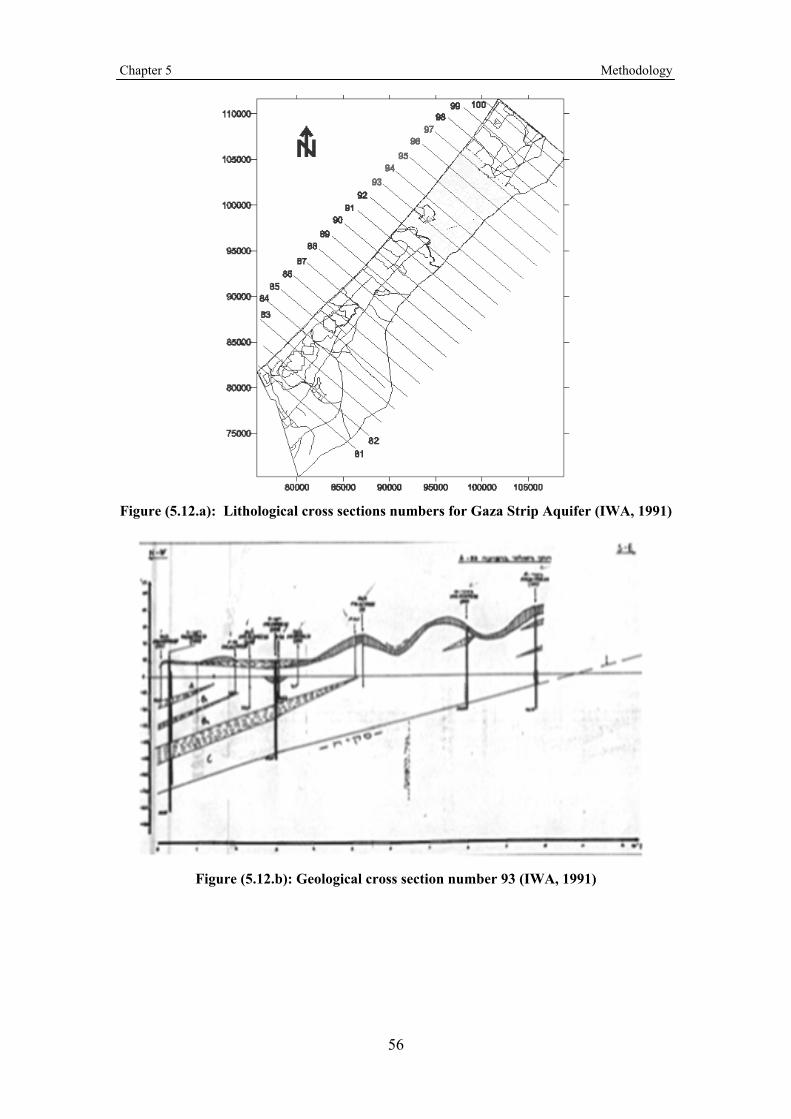
Chapter 5 Methodology
56
Figure (5.12.a): Lithological cross sections numbers for Gaza Strip Aquifer (IWA, 1991)
Figure (5.12.b): Geological cross section number 93 (IWA, 1991)
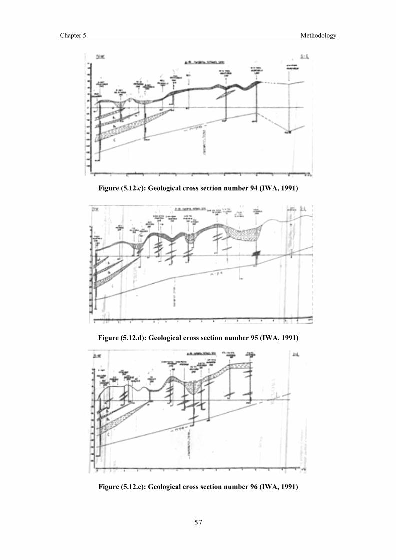
Chapter 5 Methodology
57
Figure (5.12.c): Geological cross section number 94 (IWA, 1991)
Figure (5.12.d): Geological cross section number 95 (IWA, 1991)
Figure (5.12.e): Geological cross section number 96 (IWA, 1991)

Chapter 5 Methodology
58
5.3 Construction Data Matrix for ANN Model
5.3.1 Selection the Variables of ANN Model
One of the critical issues in training the ANN model is to select input variables that are highly correlated with studied problem. The choice of variables (at least initially) is guided by intuition. Understanding and expertise in the problem domain and conditions gives initially idea of which input variables are likely to be influential. Once in ANN, variables can be selected and deselect, and ANN can also determine useful variables (Jiang and Cotton, 2004).
Hydrogeologically, the change of chloride concentration (salinity) depends on many variables such as infiltration, abstraction, life time of abstraction from aquifer, groundwater level, aquifer depth, aquifer thickness, and distance from sea shore line. These variables were discussed in previous sections. They were chosen to predict the chloride concentration which is a dependent of other variables. The chosen variables are described in Table (5.9).
Table (5.9): The variables of ANN model
Variable Sym. Unit Type
1 Final chloride concentration Clf mg/l Dependent
2 Initial chloride concentration Clo mg/l Independent
3 Recharge rate R mm/m2/month Independent
4 Abstraction Q m3/hour Independent
5 Abstraction average rate Qr mm/m2/month Independent
6 Life time Lt y Independent
7 Groundwater level Wl m Independent
8 Depth from surface to well Dw m Independent
9 Aquifer thickness Th m Independent
10 Distance from sea shore line Ds km Independent
The ANN model operated under black box, that includes large number of complex mathematical functions as discussed in Chapter 3. Equation (5.3) represents -in simple way- the ANN model.
Clf = f (Clo, R, Q, Qr, Lt, Wl, Dw, Th, Ds) (5.3)
5.3.2 Time Distribution Phases of ANN Model Data
The model data were extracted mainly from domestic wells in Gaza Strip because they usually have records of chloride concentration twice a year in February and October periodically. The time distribution divides the year in two phases A and B. The phase A starts from April to September and the phase B starts from October to March in next year. For example, time phase 1997-A extends from April 1997 to September 1997 , time phase 1997-B extends from October 1997 to March 1998 and

Chapter 5 Methodology
59
time phase 1998-A extends from April 1998 to September 1998, etc. So all other factors were organized according to this time distribution. Table (5.10) presented the time distribution phase of the ANN model for the years 1997 and 1998
Table (5.10) The time distribution phase of the ANN model for the years 1997 and 1998
Year Month Time phase 1997 April 1997 May 1997 June 1997 July 1997 August 1997 September
1997-A
1997 October 1997 November 1997 December 1998 January 1998 February 1998 March
1997-B
1998 April 1998 May 1998 June 1998 July 1998 August 1998 September
1998-A
5.3.3 Organizing of ANN Model Data
The organizing of ANN model data are required to construct some hundreds of data cases of input and output variables. These cases construct data matrix. Data organizing was carried out using software Ms. Excel and Access software. The data matrix is considered as row material to ANN model. Table (5.11) summarizes procedures of organizing ANN model variables.
Table (5.11): The procedures of organizing ANN model variables
Variable Sym. Organizing procedures
1 Final chloride concentration
Clf It is collected from PWA data bank. It is presented in Annex 2.
2 Initial chloride concentration
Clo It is collected from PWA data bank. It is presented in Annex 2.

Chapter 5 Methodology
60
3 Recharge rate R
It is calculated for each month as noticed in section 5.2.3.4 then it is summed to each time phase and the monthly rate was calculated. It is presented in Annex 3.
4 Abstraction Q
Monthly abstraction quantities for study well is collected from PWA data bank. Then it is summed for each time phase and the hourly rate was calculated. It is presented in Annex 4.
5 Abstraction average rate
Qr
It was calculated for each governate in Gaza Strip by summation of all municipal abstraction quantities and divide it to the each governate area for each time phase.
It is presented in Annex 5.
6 Life time Lt
It is calculated directly by subtracting the year of operation from the time phase year. It is presented in Annex 1.
7 Groundwater level Wl It is collected from PWA data bank. It is presented in Annex 1.
8 Depth from surface to well screen
Dw
It is calculated directly by subtracting the level of well screen from the Z coordinate of study wells. It is presented in Annex 1.
9 Aquifer thickness Th It is calculated for each well as noticed in section 5.2.8.2. It is presented in Annex 1.
10 Distance from sea shore line
Ds It is measured using Arc View program. It is presented in Annex 1.
By application the procedures in Table (5.11), the data matrix for ANN model were
obtained. The entire data matrix are presented in Annex 6. Table (5.12) presented a
side of ANN model matrix.

Chapter 5 Methodology
61
Table (5.12) Side of ANN model matrix.
Time phase
Well Clo R Q Qr Ot Wl Dw Th Ds Clf Clf-
predicted
1997-A D/67 78.0 2.14 48.23 18.71 20 -2 79 80 2.4 55.0 95.7
1997-A E/61 66.0 1.93 34.06 18.71 23 -1 43 40 1.3 145.0 120.1
1997-A A/185 70.0 1.93 172.86 18.71 14 -2 80 95 3.6 100.0 61.2
1997-A C/127 92.0 1.93 61.36 18.71 32 0 75 115 5.6 100.0 85.9
1997-A D/74 56.0 1.93 139.37 18.71 0 -2 81 50 2.0 65.0 74.9
1997-A D/68 92.0 1.93 177.38 18.71 9 -2 72 58 2.6 122.0 101.6
1997-A D/60 142.0 1.93 56.81 18.71 38 -2 45 43 3.3 129.0 183.4
1997-A C/79 427.0 0.96 0.00 18.71 27 0 64 90 6.4 384.0 438.6
1997-A E/4 108.0 1.93 81.63 18.71 37 -1 34 124 4.7 100.0 94.4
1997-A E/154 189.0 1.93 180.31 28.48 22 -2 92 50 1.7 180.0 222.3
1997-A C/128 234.0 0.96 118.65 18.71 13 1 110 86 7.7 259.0 221.2
1997-A E/157 142.0 1.93 198.43 18.71 11 -2 38 58 2.6 158.0 145.8
1997-A E/156 135.0 1.93 151.75 18.71 17 -1 70 80 4.2 135.0 131.9
1997-A E/90 142.0 1.93 74.01 18.71 27 -1 70 50 3.6 158.0 172.1
1997-A R/162B 1295.0 1.42 188.15 28.48 31 -1 70 30 1.7 1505.0 1472.7
1997-A R/162LA 262.0 1.35 126.23 28.48 11 -1 56 30 1.6 273.0 290.0
1997-A R/162G 440.0 1.93 196.53 28.48 33 -1 90 70 2.3 489.0 476.4
1997-A R/25A 397.0 1.35 116.88 28.48 17 -1 85 109 4.4 446.0 379.8
1997-A R/25D 600.0 1.35 181.30 28.48 25 -1 50 109 4.5 619.0 627.0
1997-A R/254 385.0 1.35 117.92 28.48 12 1 46 36 1.4 417.0 409.5
1997-A S/69 365.0 0.29 96.78 16.36 15 -1 73 71 5.1 417.0 375.3
1997-A J/146 517.0 0.29 95.09 16.36 13 -1 62 78 4.8 540.0 549.6
5.3.4 Analysis of ANN Model Data
Considering only those cases that have complete numeric values for all
variables without any missing data, only 499 cases satisfy the above-mentioned
criteria from 1997 to 2003. ANN model might perform well over an entire space only
when the training data are evenly distributed in the space. As the current data are
collected from limited sources (56 municipal wells), they may constitute clusters.
Therefore, the distribution of each variables across its range in the database is
examined.
The frequency distribution of different variables studied across the range of
the 499 cases are represented graphically as histograms with normal distribution curve
in Figure (5.13). The mean, standard deviation and ranges of different variables used
to train the ANN is shown in Table (5.13). The entire data matrix are presented in
Appendix 6.

Chapter 5 Methodology
62
Table (5.13): Mean , standard deviation and ranges of variables used to train the
ANN model
Range Variable Sym. Unit Mean
Std.
Dev Min. Max.
Initial chloride concentration Clo mg/l 333.07 253.94 28.00 1412.00
Recharge rate R mm/m2/month 18.19 24.44 0.00 83.07
Abstraction Q m3/hour 105.55 57.99 0.00 254.94
Abstraction average rate Qr mm/m2/month 22.50 5.80 11.37 33.94
Life time Lt y 22.02 13.94 0.00 60.00
Groundwater level Wl m -1.16 1.15 -4.00 1.00
Depth from surface to well screen
Dw m 65.26 22.05 18.00 110.00
Aquifer thickness Th m 64.17 27.25 30.00 124.00
Distance from sea shore line Ds km 3.38 1.47 0.60 7.70
Final chloride concentration Clf mg/l 341.11 261.09 35.00 1744.10
Clo = 499*200*normal(x; 333.0711; 253.939)
-200 0 200 400 600 800 1000 1200 1400 1600
Clo
0
20
40
60
80
100
120
140
160
180
200
220
240
No
of
ob
s
Figure (5.13.a): Frequency distribution of initial chloride concentration (Clo)
R = 499*10*normal(x; 18.1945; 24.4427)
-10 0 10 20 30 40 50 60 70 80 90 100
R
0
50
100
150
200
250
300
No
of
ob
s
Figure (5.13.b): Frequency distribution of recharge rate (R)

Chapter 5 Methodology
63
Q = 499*50*normal(x; 105.5514; 57.9869)
-50 0 50 100 150 200 250 300
Q
0
20
40
60
80
100
120
140
160
180
No
of
ob
s
Figure (5.13.c): Frequency distribution of
abstraction (Q)
Qr = 499*2*normal(x; 22.5001; 5.8025)
8 12 16 20 24 28 32 36
Qr
0
10
20
30
40
50
60
70
80
90
100
No
of o
bs
Figure (5.13.d): Frequency distribution of
abstraction average rate (Qr)
Lt = 499*5*normal(x; 22.016; 13.9375)
-10 0 10 20 30 40 50 60 70
Lt
0
10
20
30
40
50
60
70
80
No
of o
bs
Figure (5.13.e): Frequency distribution of life time
(Lt)
Wl = 499*1*normal(x; -1.1623; 1.1476)
-4 -3 -2 -1 0 1
Wl
0
20
40
60
80
100
120
140
160
180
200
No
of o
bs
Figure (5.13.f): Frequency distribution of
groundwater level (Wl) Dw = 499*10*normal(x; 65.2625; 22.0522)
0 10 20 30 40 50 60 70 80 90 100 110 120
Dw
0
20
40
60
80
100
120
No
of o
bs
Figure (5.13.g): Frequency distribution of depth
from surface to well screen (Dw)
Th = 499*10*normal(x; 64.1663; 27.2484)
20 30 40 50 60 70 80 90 100 110 120 130 140
Th
0
10
20
30
40
50
60
70
80
90
100
No
of o
bs
Figure (5.13.h): Frequency distribution of
aquifer thickness (Th)

Chapter 5 Methodology
64
Ds = 499*1*normal(x; 3.3808; 1.4738)
-1 0 1 2 3 4 5 6 7 8 9
Ds
0
20
40
60
80
100
120
140
160
180
No
of
ob
s
Figure (5.13.i): Frequency distribution of distance from sea shore line (Ds)
Clf = 499*200*normal(x; 341.1055; 261.089)
-200 0 200 400 600 800 1000 1200 1400 1600 1800 2000
CLf
0
20
40
60
80
100
120
140
160
180
200
220
240
No
of
ob
s
Figure (5.13.j): Frequency distribution of final
chloride concentration (Clf)
Fig (5.13): Frequency distribution of the variables across the range of 499 cases
5.4 Procedural Steps in Building ANN Model
The ANN model was designed using the STATISTICA Neural Networks (SNN) which built in STATISTICA program version 7. STATISTICA, is a program where every analysis needed is at fingertips. Used around the world in more than 20 countries, StatSoft's STATISTICA line of software has gained unprecedented recognition by users and reviewers. In addition to both basic and advanced statistics, STATISTICA products offer specialized tools for analyzing neural networks, determining sample size, designing experiments, creating real-time quality control charts, reporting via the Web, and much more of the possibilities.
The procedural steps in building and applying for ANN model varies according to the tool used in building ANN models. Using SNN, the procedural steps involves the following procedures:
5.4.1 Data Importation
Feed the data matrix for SNN to train the Network by “importing” or through the data entry process. The data must be in acceptable format such as spreadsheet. The input data is the cases that the network use to train itself.
5.4.2 Problem Definition
Specify the inputs (Independent) and the output (Dependent) variable for the ANN model. Initially, there are nine inputs variables and one output variables as mentioned in Table (5.9).
5.4.3 Extraction of the Test Set
In SNN, The test set extraction is about 50% of cases for training. 25% for calibration and 25% for testing and it is randomly selected and the user can change these percentage. Test set provide a means by which the network knows when to stop training and used for calibration and Testing.

Chapter 5 Methodology
65
5.4.4 Network Design
Choose the appropriate architecture of network among the available networks based on the type of the data and the problem. This step was previously presented in section 3.6. After many trials, Multilayer Perceptron network (MLP) has been chosen because of its high capabilities to generalize well in problems plagued with significant heterogeneity and nonlinearity.
5.4.5 Network Training
Once the type of network has been chosen, the conditions to stop training processes was set before the network is trained. Training was controlled by some of conditions as: the maximum number of iterations, target performance which specifies the tolerance between the neural network prediction and actual output, the maximum run time and the minimum allowed gradient and .The overall training of the ANN will involve the following processes; the input values of the first layer are weighted and passed on to the hidden layer; the neurons in the hidden layer will produce outputs by applying an activation function to the sum of the weighted input values; the resulting outputs are then weighted by the connections between the hidden and output layer. The desired results are generated in the output layer.
The network achieves the desired learning by adjusting its interconnected weights continuously until there is a close match between the output from the neurons and the output from the training data. The difference between the predicted outputs and the original outputs is referred to as error.
5.4.6 Network Calibration
A trained network will continuously train in order to make a model perform best on the training set. However, after some time, it is very possible for the network to “memorize” the training set instead of learning it. In order to prevent the possibility of memorization to occur, calibration is utilized. Calibration is a parameter, which indicates that the network has trained enough thus stopping the iteration process. This can be achieved in two ways;
5.4.6.1 Calibration Based on Best Test Set
When training begins at the interval specified, the Network stops to read the test set and computes an average error for it. The error of the training set continues to decrease until it becomes flat whereas the test set error decreases to an optimal point after which it slowly increases. The Network could be saved at this optimal point based on the best test set.
5.4.6.2 Calibration Based on Minimum Error Events
Training was ordered to stop when the number of invents since minimum error for test set reaches a particular value. Calibration thus prevents over training of the network and thus reduces the training time.
5.4.7 Testing of Network
After the network has been successfully trained well, it is then tested against a set of cases withheld from it during its training session. The ANN is then ready to be applied to any other values of variables.
The results are then presented in statistical manner. Regression analysis is utilized to measure the degree of correlation between the actual output and the

Chapter 5 Methodology
66
network output. Correlation factor (r) of 1 gives an indication of a perfect model while an (r) of 0 indicates a very bad model. Mathematically the values of (r) represented in equation (5.4). Detailed description for new built ANN model are presented in Chapter (6).
(5.4)
5.4.8 Application of the Network:
The built Network is then applied to any other values of input variables. The results can be displayed in statistical form to determine the correlation between the actual output and the predicted output. Detailed description about building and application ANN model are presented in Chapter (6).

Chapter 6 Results and Discussions
67
Chapter (6)
Results and Discussion
6.1 Introduction
In this chapter, the procedural steps in building ANN model was applied in order to create new ANN model able to predict chloride concentration using the input variables which discussed in Chapter (5).
Many trials were applied to get best performance model. The initial modeling trials were made using all input variables. From created ANN models, the importance and effect of each variables was studied and represented, also the sensitivity analysis was applied. Depending on the results of ANN models some input variables were neglected and new modeling trials are made without using neglected input variables. The predicted values of chloride concentration were compared with the observed values of chloride concentration and the results presented in contour maps.
6.2 Characters of Initial ANN Model
6.2.1 Topology of ANN
Several ANN models were created and tested using SNN by varying the neural networks type, the number of hidden layers, number of neurons in hidden layers and stop training conditions parameters.
After a number of trials, the best neural network was determined to be Radial Basis Function networks (RBF) with three layers: an input layer of 9 neurons, one hidden layer with 44 neurons and the output layer with 1 neuron as shown in Figure (6.1). The nine input neurons are: initial chloride concentration (CLo), recharge rate (R), abstraction (Q), abstraction average rate of area (Qr), life time (Lt), aquifer thickness (Th), groundwater level (Wl), depth from surface to well screen (Dw), and distance from sea shore line (Ds). The output neuron gives the final chloride concentration (CLf). Figure (6.1)presented the topology of the ANN model.
6.2.2 Performance of ANN
The progress of the training was checked by plotting the training, and test mean square errors versus the performed number of iterations, Figure (6.2) presented the progress of the training proceses.

Chapter 6 Results and Discussions
68
Figure (6.1): Topology of the ANN model
Training Graph
ErrorTrainingCalibration
-20 -10 0 10 20 30 40 50 60 70 80 90 100 110 120-0.04
-0.02
0.00
0.02
0.04
0.06
0.08
0.10
0.12
0.14
0.16
0.18
0.20
0.22
0.24
0.26
0.28
0.30
0.32
0.34
Figure (6.2): Training progress of ANN
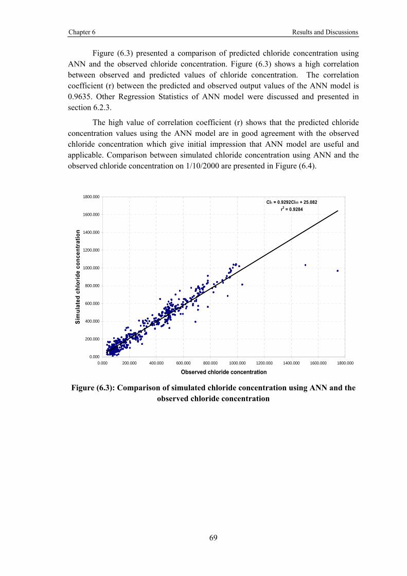
Chapter 6 Results and Discussions
69
Figure (6.3) presented a comparison of predicted chloride concentration using ANN and the observed chloride concentration. Figure (6.3) shows a high correlation between observed and predicted values of chloride concentration. The correlation coefficient (r) between the predicted and observed output values of the ANN model is 0.9635. Other Regression Statistics of ANN model were discussed and presented in section 6.2.3.
The high value of correlation coefficient (r) shows that the predicted chloride concentration values using the ANN model are in good agreement with the observed chloride concentration which give initial impression that ANN model are useful and applicable. Comparison between simulated chloride concentration using ANN and the observed chloride concentration on 1/10/2000 are presented in Figure (6.4).
Cls = 0.9292Clob + 25.082
r2 = 0.9284
0.000
200.000
400.000
600.000
800.000
1000.000
1200.000
1400.000
1600.000
1800.000
0.000 200.000 400.000 600.000 800.000 1000.000 1200.000 1400.000 1600.000 1800.000
Observed chloride concentration
Sim
ula
ted
ch
lori
de
con
cen
trat
ion
Figure (6.3): Comparison of simulated chloride concentration using ANN and the observed chloride concentration
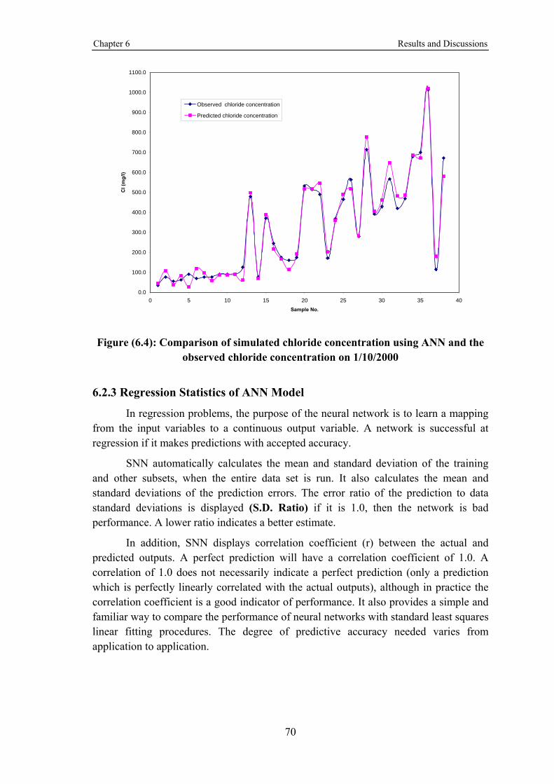
Chapter 6 Results and Discussions
70
0.0
100.0
200.0
300.0
400.0
500.0
600.0
700.0
800.0
900.0
1000.0
1100.0
0 5 10 15 20 25 30 35 40
Sample No.
Cl
(mg
/l)
Observed chloride concentration
Predicted chloride concentration
Figure (6.4): Comparison of simulated chloride concentration using ANN and the observed chloride concentration on 1/10/2000
6.2.3 Regression Statistics of ANN Model
In regression problems, the purpose of the neural network is to learn a mapping from the input variables to a continuous output variable. A network is successful at regression if it makes predictions with accepted accuracy.
SNN automatically calculates the mean and standard deviation of the training and other subsets, when the entire data set is run. It also calculates the mean and standard deviations of the prediction errors. The error ratio of the prediction to data standard deviations is displayed (S.D. Ratio) if it is 1.0, then the network is bad performance. A lower ratio indicates a better estimate.
In addition, SNN displays correlation coefficient (r) between the actual and predicted outputs. A perfect prediction will have a correlation coefficient of 1.0. A correlation of 1.0 does not necessarily indicate a perfect prediction (only a prediction which is perfectly linearly correlated with the actual outputs), although in practice the correlation coefficient is a good indicator of performance. It also provides a simple and familiar way to compare the performance of neural networks with standard least squares linear fitting procedures. The degree of predictive accuracy needed varies from application to application.

Chapter 6 Results and Discussions
71
Regression statistics are listed as follows:
Data Mean: Average value of the target output variable.
Data S.D.: Standard deviation of the target output variable.
Error Mean: Average error (residual between target and actual output values) of the output variable.
Abs. E. Mean: Average absolute error (difference between target and actual output values) of the output variable.
Error S.D.: Standard deviation of errors for the output variable.
S.D. Ratio: The error/data standard deviation ratio.
Correlation: The correlation coefficient (r) between the predicted and observed output values.
Table (6.1) present the values of regression statistics for the ANN model.
Table (6.1): The values of regression statistics for the ANN model
Regression
statistics
All model
data
Training
data set
Validation
data set
Test
data set
Data Mean 341.1055 341.0527 361.3853 320.9324
Data S.D. 260.8273 259.5903 288.6549 230.7053
Error Mean 0.9367 0.0000 -3.4865 7.2561
Error S.D. 69.8102 57.5839 95.6191 60.7904
Abs E. Mean 44.3608 39.1642 54.0085 45.2320
S.D. Ratio 0.2676 0.2218 0.3313 0.2635
Correlation (r) 0.9635 0.9751 0.9439 0.9657
It was noted that the values of regression statistics for the ANN model refers that performance of ANN model is excellent as follows:
Low value of S.D. Ratio shows that the error between observed and predicted chloride concentration values using the ANN model are small.
High value of correlation coefficient (r) shows that the predicted chloride concentration values using the ANN model are in good agreement with the observed chloride concentration.
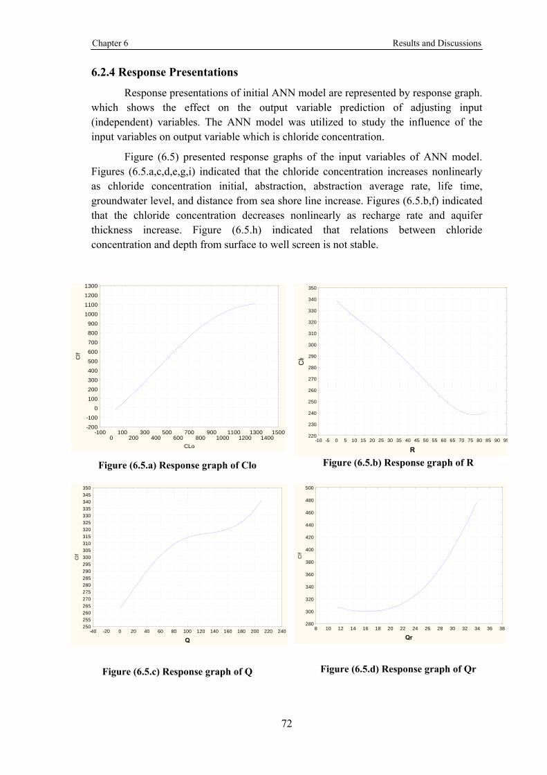
Chapter 6 Results and Discussions
72
6.2.4 Response Presentations
Response presentations of initial ANN model are represented by response graph. which shows the effect on the output variable prediction of adjusting input (independent) variables. The ANN model was utilized to study the influence of the input variables on output variable which is chloride concentration.
Figure (6.5) presented response graphs of the input variables of ANN model. Figures (6.5.a,c,d,e,g,i) indicated that the chloride concentration increases nonlinearly as chloride concentration initial, abstraction, abstraction average rate, life time, groundwater level, and distance from sea shore line increase. Figures (6.5.b,f) indicated that the chloride concentration decreases nonlinearly as recharge rate and aquifer thickness increase. Figure (6.5.h) indicated that relations between chloride concentration and depth from surface to well screen is not stable.
-1000
100200
300400
500600
700800
9001000
11001200
13001400
1500
CLo
-200
-100
0
100
200
300
400
500
600
700
800
900
1000
1100
1200
1300
Clf
Figure (6.5.a) Response graph of Clo
-10 -5 0 5 10 15 20 25 30 35 40 45 50 55 60 65 70 75 80 85 90 95
R
220
230
240
250
260
270
280
290
300
310
320
330
340
350
Clf
Figure (6.5.b) Response graph of R
-40 -20 0 20 40 60 80 100 120 140 160 180 200 220 240
Q
250
255
260
265
270
275
280
285
290
295
300
305
310
315
320
325
330
335
340
345
350
Clf
Figure (6.5.c) Response graph of Q
8 10 12 14 16 18 20 22 24 26 28 30 32 34 36 38
Qr
280
300
320
340
360
380
400
420
440
460
480
500
Clf
Figure (6.5.d) Response graph of Qr

Chapter 6 Results and Discussions
73
-10 -5 0 5 10 15 20 25 30 35 40 45 50 55 60 65 70
Lt
280
290
300
310
320
330
340
350
360
370
380
390
400
410C
lf
Figure (6.5.e) Response graph of Lt
20 30 40 50 60 70 80 90 100 110 120 130 140
Th
170
180
190
200
210
220
230
240
250
260
270
280
290
300
310
320
330
340
Clf
Figure (6.5.f) Response graph of Th
-5.0 -4.5 -4.0 -3.5 -3.0 -2.5 -2.0 -1.5 -1.0 -0.5 0.0 0.5 1.0 1.5
Wl
180
200
220
240
260
280
300
320
340
360
380
400
420
Clf
Figure (6.5.g) Response graph of Wl
0 10 20 30 40 50 60 70 80 90 100 110 120
Dw
310
315
320
325
330
335
340
345
350
355
360
Clf
Figure (6.5.h) Response graph of Dw
-0.5 0.0 0.5 1.0 1.5 2.0 2.5 3.0 3.5 4.0 4.5 5.0 5.5 6.0 6.5 7.0 7.5 8.0 8.5
Ds
280
290
300
310
320
330
340
350
360
370
380
390
400
410
420
430
Clf
Figure (6.5.i) Response graph of Ds
Figure (6.5): Response graph of input variables for initial ANN

Chapter 6 Results and Discussions
74
6.2.5 Sensitivity Analysis
SNN conducts a sensitivity analysis on the inputs to a neural network. This indicates which input variables are considered most important by that particular neural network. Sensitivity analysis can be used purely for informative purposes. Sensitivity analysis can give important insights into the usefulness of individual variables. It often identifies variables that can be safely ignored in subsequent analyses, and key variables that must always be retained. However, it must be deployed with some care, for reasons that are explained below.
Input variables are not, in general, independent - that is, there are interdependencies between variables. Sensitivity analysis rates variables according to the deterioration in modeling performance that occurs if that variable is no longer available to the model. In so doing, it assigns a single rating value to each variable. However, the interdependence between variables means that no scheme of single ratings per variable can ever reflect the subtlety of the true situation.
Consider, for example, the case where two input variables encode the same information (they might even be copies of the same variable). A particular model might depend wholly on one, wholly on the other, or on some arbitrary combination of them. Then sensitivity analysis produces an arbitrary relative sensitivity to them. Moreover, if either is eliminated the model may compensate adequately because the other still provides the key information. It may therefore rate the variables as of low sensitivity, even though they might encode key information. Similarly, a variable that encodes relatively unimportant information, but is the only variable to do so, may have higher sensitivity than any number of variables that mutually encode more important information.
SNN conducts sensitivity analysis by treating each input variable in turn as if it were "unavailable". SNN has defined a missing value substitution procedure, which is used to allow predictions to be made in the absence of values for one or more inputs. To define the sensitivity of a particular variable, v, the network first was run on a set of test cases, and the network error was accumulated. Then the network was run again using the same cases, but this time replacing the observed values of v with the value estimated by the missing value procedure, and again the network error was accumulated. (STATISTICA, 2004).
After that, It is expected some deterioration in error to occur. The basic measure of sensitivity is the ratio of the error with missing value substitution to the original error. The more sensitive the network is to a particular input, the greater the deterioration we can expect, and therefore the greater the ratio. Once sensitivities have been calculated for all variables, they may be ranked in order. SNN provides these rankings, for convenience in interpreting the sensitivities. Table (6.2) presented the value of error Ratio Rank of input variables.

Chapter 6 Results and Discussions
75
Table (6.2): The value of error ratio and rank of input variables
Variables Clo R Q Qr Lt Th Wl Dw Ds
Error Ratio 3.08 1.04 1.05 1.09 1.10 1.08 1.02 1.07 0.99
Variables Rank 1 7 6 3 2 4 8 5 9
Training error ratio 3.62 1.05 1.18 1.17 1.22 1.12 1.04 1.11 1.01
Training variables Rank 1 7 3 4 2 5 8 6 9
Validation error ratio 2.64 1.02 0.95 1.02 1.06 1.03 1.01 1.05 0.96
Validation variables Rank 1 6 9 5 2 4 7 3 8
Test error ratio 3.06 1.06 1.03 1.11 1.00 1.15 1.02 1.06 1.02
Test variables Rank 1 4 6 3 9 2 8 5 7
It was noted that value of Error Ratio of the initial chloride concentration (Clo) is the highest value of Error Ratio which mean that the final Chloride concentration (Clf) is high correlated to initial chloride concentration (Clo). The most other important variables for this model is life time (Lt), abstraction average rate of area (Qr) and aquifer thickness (Th). Other variables rank are presented in Table (6.2).
6.2.6 Determination the Real Importance of Input Variables
Sensitivity analysis does not rate the "usefulness" of variables in modeling in a reliable or absolute manner. The cautious is needed during drawing the conclusions about the importance of variables. Nonetheless, in practice it is extremely useful. If a number of models are studied, it is often possible to identify key variables that are always of high sensitivity, others that are always of low sensitivity and "ambiguous" variables that change ratings and probably carry mutually redundant information (SNN, 2004).
To determine the real importance and ranking of variables, twenty ANN models were created and sensitivity analysis was applied and results of sensitivity analysis were presented in Table (6.3).
Table (6.3): Sensitivity analysis of twenty ANN models
Model No.
Clo R Q Qr Lt Th Wl Dw Ds
1 2.95 1.02 1.00 0.98 0.98 0.98 0.98 1.02 1.01
2 3.22 1.02 0.98 1.06 1.01 1.00 0.99 1.02 1.04
3 3.52 1.00 1.04 1.01 1.02 1.04 1.03 0.98 1.04
4 3.00 0.99 1.00 0.99 1.01 1.02 1.01 0.98 0.99
5 3.14 0.99 1.00 0.98 0.99 0.99 1.00 0.98 0.96

Chapter 6 Results and Discussions
76
6 3.06 1.00 1.00 1.01 1.01 1.00 1.00 0.98 0.95
7 3.51 0.99 1.00 1.02 1.03 1.02 1.00 1.00 0.96
8 3.27 1.00 1.00 1.00 1.01 0.98 1.00 0.99 0.97
9 3.54 0.99 1.01 0.99 1.02 1.01 1.01 1.00 0.97
10 3.51 1.01 1.01 1.02 1.04 0.99 1.00 0.99 0.99
11 2.72 1.01 1.00 1.04 0.98 1.04 1.02 0.97 0.98
12 2.96 0.99 1.05 1.08 0.98 1.02 1.04 0.99 0.98
13 3.09 1.00 1.01 1.12 1.03 1.15 1.03 0.97 1.03
14 3.08 1.04 1.05 1.09 1.10 1.08 1.02 1.07 0.99
15 3.23 1.02 1.01 1.02 0.98 0.98 1.01 1.00 0.97
16 3.57 1.01 1.01 1.09 1.00 1.06 1.01 1.04 1.01
17 3.65 1.04 1.00 1.04 1.01 1.04 1.01 1.03 0.98
18 3.74 1.02 1.01 1.08 1.01 1.06 1.02 1.02 1.00
19 4.10 1.05 1.01 1.05 1.05 1.03 1.04 1.01 1.00
20 4.24 1.05 1.04 1.08 1.05 1.01 1.01 1.02 1.02
Total 67.10 20.26 20.23 20.73 20.32 20.49 20.23 20.07 19.85
Average 3.355 1.013 1.012 1.037 1.016 1.024 1.011 1.004 0.992
Rank 1 6 5 2 4 3 7 8 9
From the results in Table (6.3), the variables can be ranked as described in Table (6.4). This rank is needed to identify variables that can be safely ignored in subsequent modeling, and key variables that must always be retained. From the result three variables with lowest sensitivity which is groundwater level (Wl), depth from surface to well screen (Dw), and distance from sea shore line (Ds) can be ignored in subsequent modeling.
Table (6.4) Rank of ANN model variables extracted from twenty ANN models
Rank Variable Action
1 Initial chloride concentration Retained
2 Abstraction average rate Retained
3 Live time Retained
4 Aquifer thickness Retained
5 Abstraction Retained
6 Recharge rate Retained
7 Ground water level Ignored
8 Depth from surface to well Ignored
9 Distance from sea shore line Ignored

Chapter 6 Results and Discussions
77
6.3 Characters of the Final ANN Model
6.3.1 Topology of ANN
Depending on the results of ANN models in Table (6.3), three input variables were neglected and new training trials are made without using neglected input variables. The neglected input variables is groundwater level, depth from surface to well screen, and distance from sea shore line.
Several ANN models were created and tested using SNN by varying the neural networks type, the number of hidden layers, number of neurons in hidden layers and stop training conditions parameters.
After a number of trials, the best neural network was determined to be Multilayer Perceptron network (MLP) with four layers: an input layer of 6 neurons, first hidden layer with 10 neurons, second hidden layer with 7 neurons and the output layer with 1 neuron as shown in Figure (6.6). The six input neurons are: initial chloride concentration (Clo), recharge rate (R), abstraction (Q), abstraction average rate of area (Qr), life time (Lt), aquifer thickness (Th). The output neuron gives the final chloride concentration (Clf).
.
Figure (6.6): Topology of final ANN model
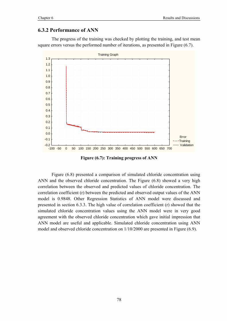
Chapter 6 Results and Discussions
78
6.3.2 Performance of ANN
The progress of the training was checked by plotting the training, and test mean square errors versus the performed number of iterations, as presented in Figure (6.7).
Training Graph
ErrorTraining Validation
-100 -50 0 50 100 150 200 250 300 350 400 450 500 550 600 650 700-0.2
-0.1
0.0
0.1
0.2
0.3
0.4
0.5
0.6
0.7
0.8
0.9
1.0
1.1
1.2
1.3
Figure (6.7): Training progress of ANN
Figure (6.8) presented a comparison of simulated chloride concentration using ANN and the observed chloride concentration. The Figure (6.8) showed a very high correlation between the observed and predicted values of chloride concentration. The correlation coefficient (r) between the predicted and observed output values of the ANN model is 0.9848. Other Regression Statistics of ANN model were discussed and presented in section 6.3.3. The high value of correlation coefficient (r) showed that the simulated chloride concentration values using the ANN model were in very good agreement with the observed chloride concentration which gave initial impression that ANN model are useful and applicable. Simulated chloride concentration using ANN model and observed chloride concentration on 1/10/2000 are presented in Figure (6.9).

Chapter 6 Results and Discussions
79
Cls = 0.9653Clob+ 15.064
r2 = 0.9698
0
200
400
600
800
1000
1200
1400
1600
1800
0 200 400 600 800 1000 1200 1400 1600 1800 2000
Observed chloride concentration
Sim
ula
ted
ch
lori
de
con
cen
trat
ion
Figure (6.8): Comparison of simulated chloride concentration using ANN model and the observed chloride concentration
0.0
100.0
200.0
300.0
400.0
500.0
600.0
700.0
800.0
900.0
1000.0
1100.0
0 5 10 15 20 25 30 35 40
Sample No.
Cl
(mg
/l)
Observed chloride concentration
Predicted chloride concentration ANN-6
Figure (6.9): Comparison of simulated chloride concentration using ANN and the observed chloride concentration on 1/10/2000

Chapter 6 Results and Discussions
80
6.3.3 Summary Regression Statistics of Final ANN Model
It was noted that the values of regression statistics for the ANN model which presented in Table (6.5) referred that performance of ANN model was excellent as follows:
Low value of Error Mean, Abs E. Mean and S.D. Ratio showed that the error between observed and simulated chloride concentration values using the ANN model are small.
High value of correlation coefficient (r) showed that the simulated chloride concentration values using the ANN model are in good agreement with the observed chloride concentration.
By comparing regression summary statistics of final an ANN model (using MLP with 6 inputs) and initial ANN model (RBF with 9 inputs), it was concluded that the performance of final ANN model is better than the performance of final ANN model.
Table (6.5): The values of regression statistics for final ANN model
Regression statistics
All model data
Training
data set
Validation data set
Test data set
Data Mean 341.105 295.877 345.200 361.427
Data S.D. 260.827 247.433 262.657 263.607
Error Mean 3.242 5.016 8.428 -0.196
Error S.D. 45.371 45.125 47.312 44.204
Abs E. Mean 29.798 29.262 32.128 28.911
S.D. Ratio 0.174 0.182 0.180 0.168
Correlation (r) 0.9848 0.9832 0.9837 0.9860
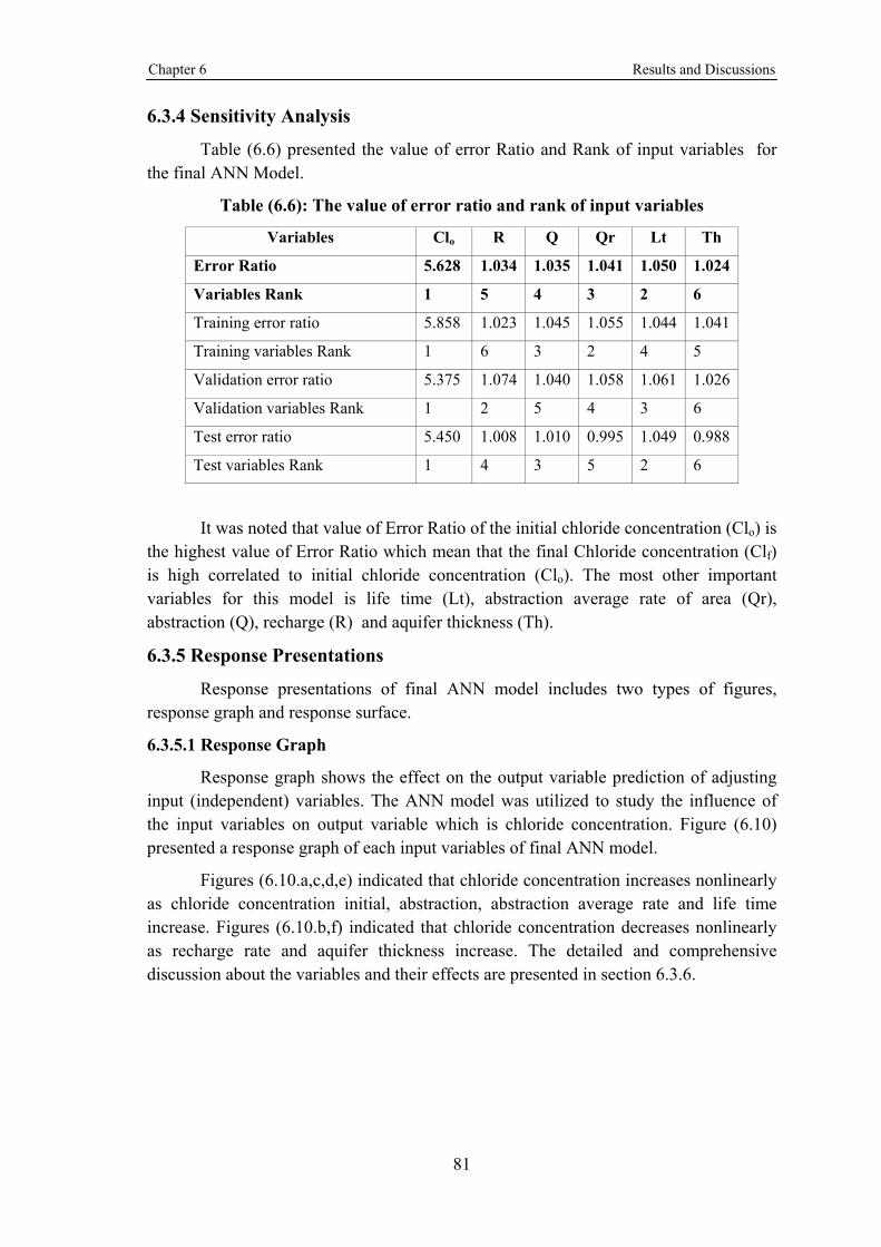
Chapter 6 Results and Discussions
81
6.3.4 Sensitivity Analysis
Table (6.6) presented the value of error Ratio and Rank of input variables for the final ANN Model.
Table (6.6): The value of error ratio and rank of input variables
Variables Clo R Q Qr Lt Th
Error Ratio 5.628 1.034 1.035 1.041 1.050 1.024
Variables Rank 1 5 4 3 2 6
Training error ratio 5.858 1.023 1.045 1.055 1.044 1.041
Training variables Rank 1 6 3 2 4 5
Validation error ratio 5.375 1.074 1.040 1.058 1.061 1.026
Validation variables Rank 1 2 5 4 3 6
Test error ratio 5.450 1.008 1.010 0.995 1.049 0.988
Test variables Rank 1 4 3 5 2 6
It was noted that value of Error Ratio of the initial chloride concentration (Clo) is the highest value of Error Ratio which mean that the final Chloride concentration (Clf) is high correlated to initial chloride concentration (Clo). The most other important variables for this model is life time (Lt), abstraction average rate of area (Qr), abstraction (Q), recharge (R) and aquifer thickness (Th).
6.3.5 Response Presentations
Response presentations of final ANN model includes two types of figures, response graph and response surface.
6.3.5.1 Response Graph
Response graph shows the effect on the output variable prediction of adjusting input (independent) variables. The ANN model was utilized to study the influence of the input variables on output variable which is chloride concentration. Figure (6.10) presented a response graph of each input variables of final ANN model.
Figures (6.10.a,c,d,e) indicated that chloride concentration increases nonlinearly as chloride concentration initial, abstraction, abstraction average rate and life time increase. Figures (6.10.b,f) indicated that chloride concentration decreases nonlinearly as recharge rate and aquifer thickness increase. The detailed and comprehensive discussion about the variables and their effects are presented in section 6.3.6.

Chapter 6 Results and Discussions
82
-200-100
0100
200300
400500
600700
800900
10001100
12001300
14001500
1600
Clo
-100
0
100
200
300
400
500
600
700
800
900
1000
1100
1200
1300
1400
1500
1600
1700
1800
Clf
Figure (6.10.a): Response graph of Clo
-10 -5 0 5 10 15 20 25 30 35 40 45 50 55 60 65 70 75 80 85 90 95
R
305
310
315
320
325
330
335
340
345
350
355
360
365
370
375
380
Clf
Figure (6.10.b): Response graph of R
-40 -20 0 20 40 60 80 100 120 140 160 180 200 220 240 260 280
Q
356
357
358
359
360
361
362
363
364
365
366
367
368
369
370
371
372
Clf
Figure (6.10.c): Response graph of Q

Chapter 6 Results and Discussions
83
8 10 12 14 16 18 20 22 24 26 28 30 32 34 36 38
Qr
330
335
340
345
350
355
360
365
370
375
380
Clf
Figure (6.10.d): Response graph of Qr
-10 -5 0 5 10 15 20 25 30 35 40 45 50 55 60 65
Lt
348
350
352
354
356
358
360
362
364
366
368
370
372
374
376
Clf
Figure (6.10.e): Response graph of Lt
20 30 40 50 60 70 80 90 100 110 120 130 140
Th
330
332
334
336
338
340
342
344
346
348
350
352
354
356
358
360
362
364
Clf
Figure (6.10.f): Response graph of Th
Figure (6.10) Response graph of each input variables of final ANN model

Chapter 6 Results and Discussions
84
6.3.5.2 Response Surface
A response surface is a figure shows the effect on the output variable prediction of adjusting two input (independent) variables. The ANN model was utilized to study the influence of each two input variables on chloride concentration. Figures (6.11) presented response surface of each two input variables of final ANN model
Figures (6.11.a) indicated that the chloride concentration increases nonlinearly as recharge decreases and abstraction increases and the effect of recharge is stronger than effect of abstraction. Figure (6.11.b) indicated that the chloride concentration increases nonlinearly as recharge decreases and abstraction average rate increases and the effect of recharge is similar to effect of abstraction average rate. Figure (6.11.c) indicated that the chloride concentration increases nonlinearly as life time increases and recharge decreases and the effect of recharge is stronger than effect of life time. Figures (6.11.d) indicated that the chloride concentration increases nonlinearly as recharge decrease and aquifer thickness and the effect of aquifer thickness is stronger than effect of recharge.
Figure (6.11.e) indicated that the chloride concentration increases nonlinearly as abstraction and abstraction average rate increase and the effect of abstraction average rate is similar to the effect of abstraction. Figure (6.11.f) indicated that the chloride concentration increases nonlinearly as abstraction and life time increase and the effect of life time is similar to effect of abstraction. Figure (6.11.g) indicated that the chloride concentration increases nonlinearly as abstraction increases and aquifer thickness decrease. In addition, it was noted that effect of aquifer thickness is stronger than effect of abstraction.
Figure (6.11.h) indicated that the chloride concentration increases nonlinearly as abstraction average rate and life time increase and the effect of abstraction average rate is stronger than effect of life time. Figure (6.11.i) indicated that the chloride concentration increases nonlinearly as abstraction average rate increases and aquifer thickness decreases and the effect of aquifer thickness is similar to effect of abstraction average rate.
Figure (6.11.j) indicated that the chloride concentration increases nonlinearly as life time increases and aquifer thickness decreases. In addition, it was noted that effect of aquifer thickness is similar to effect of life time.

Chapter 6 Results and Discussions
85
Figure (6.11.a) Response surface of R & Q
Figure (6.11.b) Response surface of R & Qr
Figure (6.11.c) Response surface of R & Lt
Figure (6.11.d) Response surface of R & Th
Figure (6.11.e) Response surface of Q & Qr
Figure (6.11.f) Response surface of Q & Lt

Chapter 6 Results and Discussions
86
Figure (6.11.g) Response surface of Q & Th
Figure (6.11.h) Response surface of Qr & Lt
Figure (6.11.i) Response surface of Th & Qr
Figure (6.11.j) Response surface of Th & Lt
Figures (6.11) Response surface of each two input variables of final ANN model
6.4 Application of ANN Model
The ANN model was utilized in many practical and theoretical applications. It was utilized as analytical tool to study the influence of the input variables on chloride concentration. Furthermore, it was utilized as simulation and prediction tool of chloride concentration on domestic wells in Gaza Strip. Finally it was utilized as a decision making support tool.
6.4.1 Utilizing ANN Model as Analytical Tool
The ANN model was utilized to study the influence of the input variables on chloride concentration. Hypothetical cases of input variables were assumed to study the
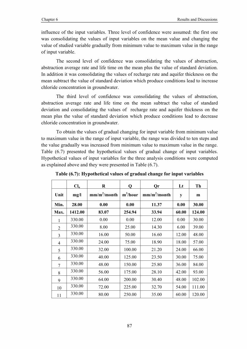
Chapter 6 Results and Discussions
87
influence of the input variables. Three level of confidence were assumed: the first one was consolidating the values of input variables on the mean value and changing the value of studied variable gradually from minimum value to maximum value in the range of input variable.
The second level of confidence was consolidating the values of abstraction, abstraction average rate and life time on the mean plus the value of standard deviation. In addition it was consolidating the values of recharge rate and aquifer thickness on the mean subtract the value of standard deviation which produce conditions lead to increase chloride concentration in groundwater.
The third level of confidence was consolidating the values of abstraction, abstraction average rate and life time on the mean subtract the value of standard deviation and consolidating the values of recharge rate and aquifer thickness on the mean plus the value of standard deviation which produce conditions lead to decrease chloride concentration in groundwater.
To obtain the values of gradual changing for input variable from minimum value to maximum value in the range of input variable, the range was divided to ten steps and the value gradually was increased from minimum value to maximum value in the range. Table (6.7) presented the hypothetical values of gradual change of input variables. Hypothetical values of input variables for the three analysis conditions were computed as explained above and they were presented in Table (6.7).
Table (6.7): Hypothetical values of gradual change for input variables
Clo R Q Qr Lt Th
Unit mg/l mm/m2/month m3/hour mm/m2/month y m
Min. 28.00 0.00 0.00 11.37 0.00 30.00
Max. 1412.00 83.07 254.94 33.94 60.00 124.00
1 330.00 0.00 0.00 12.00 0.00 30.00
2 330.00 8.00 25.00 14.30 6.00 39.00
3 330.00 16.00 50.00 16.60 12.00 48.00
4 330.00 24.00 75.00 18.90 18.00 57.00
5 330.00 32.00 100.00 21.20 24.00 66.00
6 330.00 40.00 125.00 23.50 30.00 75.00
7 330.00 48.00 150.00 25.80 36.00 84.00
8 330.00 56.00 175.00 28.10 42.00 93.00
9 330.00 64.00 200.00 30.40 48.00 102.00
10 330.00 72.00 225.00 32.70 54.00 111.00
11 330.00 80.00 250.00 35.00 60.00 120.00

Chapter 6 Results and Discussions
88
Table (6.8): Hypothetical values of input variables for the three analysis conditions
Clo R Q Qr Lt Th
Min. 28.00 0.00 0.00 11.37 0.00 30.00
Max. 1412.00 83.07 254.94 33.94 60.00 124.00
Mean 333.07 18.19 105.55 22.50 22.02 64.17
S.D 253.94 24.44 57.99 5.80 13.94 27.25
M+S.D 587.01 42.64 163.54 28.30 35.95 91.41
M-S.D 79.13 -6.25 47.56 16.70 8.08 36.92
Normal Condition 330.00 18.00 105.00 22.00 22.00 65.00
Decreasing Condition 330.00 0.00 164.00 29.00 36.00 40.00
Increasing Condition 330.00 43.00 47.00 16.00 8.00 91.00
6.4.1.1 Influence of Recharge Rate on Chloride Concentration
By application the above mentioned procedure and using the final ANN model to calculate the value of final chloride concentration for each hypothetical case, the effect of recharge rate on chloride concentration was studied. Results of the three conditions (normal, increasing and decreasing) were presented in Figure (6.12) and Table (6.9) and Table (6.10).
Fig (6.12): Impact of recharge rate on chloride concentration
(mm/m2/month)

Chapter 6 Results and Discussions
89
Table (6.9): Results of ANN model for hypothetical cases studied the effect of recharge rate on chloride concentration
Normal Condition
Clo R Q Qr Lt Th Clf
1 330.00 0.00 105.00 22.00 22.00 65.00 346.00
2 330.00 8.00 105.00 22.00 22.00 65.00 342.11
3 330.00 16.00 105.00 22.00 22.00 65.00 337.45
4 330.00 24.00 105.00 22.00 22.00 65.00 332.21
5 330.00 32.00 105.00 22.00 22.00 65.00 326.58
6 330.00 40.00 105.00 22.00 22.00 65.00 320.70
7 330.00 48.00 105.00 22.00 22.00 65.00 314.71
8 330.00 56.00 105.00 22.00 22.00 65.00 308.67
9 330.00 64.00 105.00 22.00 22.00 65.00 302.67
10 330.00 72.00 105.00 22.00 22.00 65.00 296.75
11 330.00 80.00 105.00 22.00 22.00 65.00 290.91
Increasing Condition
Clo R Q Qr Lt Th Clf
1 330.00 0.00 164.00 29.00 36.00 40.00 363.06
2 330.00 8.00 164.00 29.00 36.00 40.00 358.88
3 330.00 16.00 164.00 29.00 36.00 40.00 354.22
4 330.00 24.00 164.00 29.00 36.00 40.00 349.20
5 330.00 32.00 164.00 29.00 36.00 40.00 343.91
6 330.00 40.00 164.00 29.00 36.00 40.00 338.45
7 330.00 48.00 164.00 29.00 36.00 40.00 332.86
8 330.00 56.00 164.00 29.00 36.00 40.00 327.19
9 330.00 64.00 164.00 29.00 36.00 40.00 321.47
10 330.00 72.00 164.00 29.00 36.00 40.00 315.71
11 330.00 80.00 164.00 29.00 36.00 40.00 309.93
Decreasing Condition
Clo R Q Qr Lt Th Clf
1 330.00 0.00 47.00 16.00 8.00 91.00 316.89
2 330.00 8.00 47.00 16.00 8.00 91.00 315.78
3 330.00 16.00 47.00 16.00 8.00 91.00 313.21
4 330.00 24.00 47.00 16.00 8.00 91.00 309.44
5 330.00 32.00 47.00 16.00 8.00 91.00 304.73
6 330.00 40.00 47.00 16.00 8.00 91.00 299.33
7 330.00 48.00 47.00 16.00 8.00 91.00 293.47
8 330.00 56.00 47.00 16.00 8.00 91.00 287.35
9 330.00 64.00 47.00 16.00 8.00 91.00 281.12
10 330.00 72.00 47.00 16.00 8.00 91.00 274.89
11 330.00 80.00 47.00 16.00 8.00 91.00 268.75

Chapter 6 Results and Discussions
90
Table (6.10): Summary of results of ANN model for hypothetical cases studied the effect of recharge rate on chloride concentration
It was noted that increasing recharge rate from 0 to 80 mm/m2/month resulted in a large influence in final chloride concentration as follows:
In normal condition, when the initial chloride concentration = 330 mg/l , abstraction =105 m3/hr, abstraction average rate = 22 mm/m2/month, life time = 22 years and aquifer thickness = 65 m. Final chloride concentration decrease from 346.00 mg/l to 290.91 mg/l. Final chloride concentration stayed stable of 330 mg/l on recharge rate of 28 mm/month.
In increasing condition, when the initial chloride concentration = 330 mg/l , abstraction =146 m3/hr, abstraction average rate = 29 mm/m2/month, life time = 36 years and aquifer thickness = 40 m. Final chloride concentration decreased from 363.06 mg/l to 309.93 mg/l. Final chloride concentration stayed stable of 330 mg/l on recharge rate of 52 mm/ m2/month.
In decreasing condition, when initial chloride concentration = 330 mg/l, abstraction = 47 m3/hr, abstraction average rate = 16 mm/m2/month, Life time = 8 years and aquifer thickness = 91 m. Final chloride concentration decreased from 316.89 mg/l to 268.75 mg/l. In this condition final chloride concentration stayed less than 330 mg/l for all values of recharge rate even if small values of recharge because of very good condition of small value of abstraction, abstraction average rate life time and large aquifer thickness.
It is noted that stabilization point of chloride concentration for normal condition occurred at recharge rate = 22 mm/m2/month and for increasing condition occurs at recharge rate = 52 mm/m2/month which mean that increasing condition required height recharge rate to achieve stabilization point of chloride concentration. In decreasing condition final chloride concentration stayed less
R Clf Clf Clf
Decreasing Normal Increasing
1 0.00 316.89 346.00 363.06
2 8.00 315.78 342.11 358.88
3 16.00 313.21 337.45 354.22
4 24.00 309.44 332.21 349.20
5 32.00 304.73 326.58 343.91
6 40.00 299.33 320.70 338.45
7 48.00 293.47 314.71 332.86
8 56.00 287.35 308.67 327.19
9 64.00 281.12 302.67 321.47
10 72.00 274.89 296.75 315.71
11 80.00 268.75 290.91 309.93

Chapter 6 Results and Discussions
91
than 330 mg/l with values 316.89 mg/l to 268.75 mg/l for all values of recharge rate even if small values of recharge rate were available.
6.4.1.2 Influence of Abstraction on Chloride Concentration
By application the above mentioned procedure and using the final ANN model to calculate the value of final chloride concentration for each hypothetical case, the effect of abstraction on chloride concentration was studied. Results of the three conditions (normal, increasing and decreasing) were presented in Figure (6.13) and Table (6.11).
Results of ANN model for hypothetical cases studied the effect of abstraction on chloride concentration are presented in Annex 7.
Fig (6.13): Effect of abstraction on chloride concentration
Table (6.11): Results of ANN model for hypothetical cases studied the effect of abstraction on chloride concentration
Q Clf Clf Clf
Decreasing Normal Increasing
1 0.00 299.29 335.6 350.68
2 25.00 298.00 335.1 351.47
3 50.00 297.08 335.0 352.75
4 75.00 296.49 335.4 354.47

Chapter 6 Results and Discussions
92
It was noted that increasing abstraction from 0 to 250 m3/hr results in a small influence in final chloride concentration as follows:
In normal condition, when the initial chloride concentration = 330 mg/l, recharge rate = 18 mm/m2/month, abstraction average rate = 22 mm/m2/month, life time = 22 years and aquifer thickness = 65 m. Final chloride concentration increases from 335.6 mg/l to 343.7 mg/l. Final chloride concentration stays more than 330 mg/l for all values of abstraction.
In increasing condition, when the initial chloride concentration = 330 mg/l , recharge rate = 0 mm/ m2/month, abstraction average rate = 29 mm/m2/month, life time = 36 years and aquifer thickness = 40 m. Final chloride concentration decrease from 350.68 mg/l to 372.74 mg/l. Final chloride concentration stays more than 330 mg/l for all values of abstraction.
In decreasing condition, when the initial chloride concentration = 330 mg/l, recharge rate = 43 mm/m2/month, Abstraction average rate = 16 mm/m2/month, life time = 8 years and aquifer thickness = 91 m. Final chloride concentration Stays almost steady at 297 mg/l which mean that in good condition of small value of Abstraction average rate and life time and large value of Recharge rate and aquifer thickness, Increasing abstraction dos not affect on the chloride concentration and it decreases about 33 mg/l which is good result.
6.4.1.3 Impacts of Abstraction Average Rate on Chloride Concentration
By application the above mentioned procedure and using the final ANN model to calculate the value of final chloride concentration for each hypothetical case, the effect of abstraction average rate on chloride concentration was studied. Results of the three conditions (normal, increasing and decreasing) were presented in Figure (6.14) and Table (6.12).
Results of ANN model for hypothetical cases studied the effect of abstraction average rate on chloride concentration are presented in Annex 7.
5 100.00 296.19 336.0 356.55
6 125.00 296.11 337.0 358.93
7 150.00 296.20 338.1 361.53
8 175.00 296.39 339.5 364.29
9 200.00 296.61 340.9 367.13
10 225.00 296.78 342.3 369.97
11 250.00 296.83 343.7 372.74
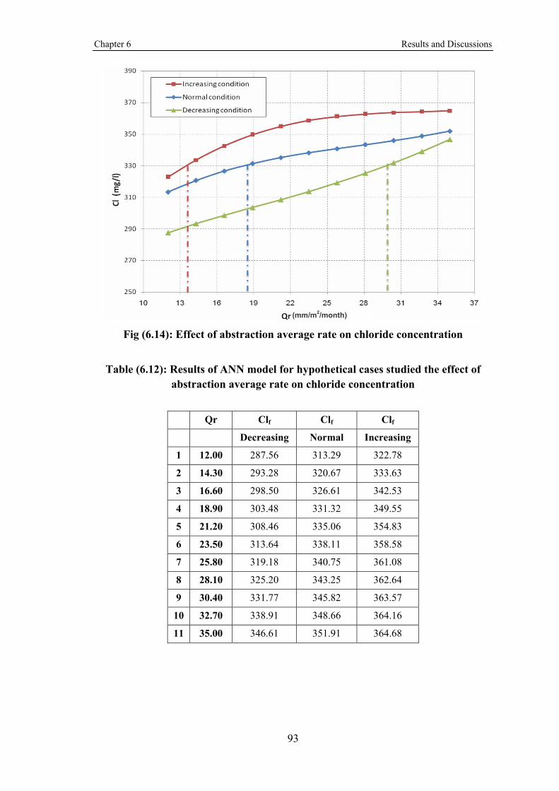
Chapter 6 Results and Discussions
93
Fig (6.14): Effect of abstraction average rate on chloride concentration
Table (6.12): Results of ANN model for hypothetical cases studied the effect of abstraction average rate on chloride concentration
Qr Clf Clf Clf
Decreasing Normal Increasing
1 12.00 287.56 313.29 322.78
2 14.30 293.28 320.67 333.63
3 16.60 298.50 326.61 342.53
4 18.90 303.48 331.32 349.55
5 21.20 308.46 335.06 354.83
6 23.50 313.64 338.11 358.58
7 25.80 319.18 340.75 361.08
8 28.10 325.20 343.25 362.64
9 30.40 331.77 345.82 363.57
10 32.70 338.91 348.66 364.16
11 35.00 346.61 351.91 364.68
(mm/m2/month)

Chapter 6 Results and Discussions
94
It was noted that increasing abstraction average rate from 12 to 35 mm/m2/month results in a large influence in final chloride concentration as follows:
In normal condition, when the initial chloride concentration = 330 mg/l , recharge rate = 18 mm/ m2/month, abstraction =105 m3/hr, life time = 22 years and aquifer thickness = 65 m. Final chloride concentration increases from 313.29 mg/l to 351.91 mg/l. Final chloride concentration stays stable and = 330 mg/l on Abstraction average rate = 18.5 mm/m2/month.
In increasing condition, when the initial chloride concentration = 330 mg/l , recharge rate = 0 mm/m2/month, abstraction =164 m3/hr, life time = 36 years and aquifer thickness = 40 m. Final chloride concentration increases from 322.78 mg/l to 364.68 mg/l. Final chloride concentration stays stable and = 330 mg/l on abstraction average rate = 14 mm/m2/month
In decreasing condition, when the initial chloride concentration = 330 mg/l, recharge rate = 43 mm/m2/month, abstraction = 47 m3/hr, Life time = 8 years and aquifer thickness = 91. Final chloride concentration increases from 287.56 mg/l to 346.61 mg/l. Final chloride concentration stays stable and = 330 mg/l on abstraction average rate = 30 mm/m2/month.
It is noted that stabilization point of chloride concentration for normal condition occurs at abstraction average rate = 18.5 mm/m2/month and for increasing condition occurs at abstraction average rate = 14 mm/m2/month and for decreasing condition occurs at abstraction average rate = 30 mm/m2/month which mean that increasing condition requires smallest abstraction average rate to achieve stabilization point of chloride concentration while decreasing condition can achieve stabilization point of chloride concentration with height value of abstraction average rate.
6.4.1.4 Influence of Life Time on Chloride Concentration
By application the above mentioned procedure and using the final ANN model to calculate the value of final chloride concentration for each hypothetical case, the effect of life time on chloride concentration was studied. Results of the three conditions (normal, increasing and decreasing) were presented in Figure (6.15) and Table (6.13).
Results of ANN model for hypothetical cases studied the effect of life time on chloride concentration are presented in Annex 7.

Chapter 6 Results and Discussions
95
Fig (6.15): Effect of life time on chloride concentration
Table (6.13): Results of ANN model for hypothetical cases studied the effect of life time on chloride concentration
Lt Clf Clf Clf
Decreasing Normal Increasing
1 0.00 291.91 326.36 358.44
2 6.00 295.91 329.36 359.32
3 12.00 299.60 332.10 360.10
4 18.00 303.00 334.61 360.82
5 24.00 306.18 336.95 361.53
6 30.00 309.17 339.15 362.26
7 36.00 312.02 341.26 363.06
8 42.00 314.76 343.33 363.97
9 48.00 317.44 345.40 365.04
10 54.00 320.09 347.50 366.30
11 60.00 322.75 349.67 367.78

Chapter 6 Results and Discussions
96
It was noted that increasing Life time from 0 to 60 year results in a large influence in final chloride concentration as follows:
In normal condition, when the initial chloride concentration = 330 mg/l , recharge rate = 18 mm/m2/month, abstraction =105 m3/hr, abstraction average rate = 22 mm/m2/month, and aquifer thickness = 65 m. Final chloride concentration increases from 326.36 mg/l to 349.67 mg/l. final chloride concentration stays stable and = 330 mg/l on life time = 7 years.
In increasing condition, when the initial chloride concentration = 330 mg/l , recharge rate = 0 mm/m2/month, abstraction =164 m3/hr, abstraction average rate = 29 mm/m2/month and aquifer thickness = 40 m. Final chloride concentration increases from 358.44 mg/l to 367.78 mg/l. Final Chloride concentration stays more than 330 mg/l for all values of life time.
In decreasing condition, when the initial chloride concentration = 330 mg/l, Recharge rate = 43 mm/m2/month, Abstraction = 47 m3/hr, abstraction average rate = 16 mm/m2/month and aquifer thickness = 91. Final chloride concentration increases from 291.91 mg/l to 322.75 mg/l. Final chloride concentration stays less than 330 mg/l for all values of life time.
It is noted that stabilization point of chloride concentration for normal condition occurs at life time = 6 year. For increasing condition, chloride concentration stays more than 330 mg/l with values from 358.44 mg/l to 367.78 mg/l and for decreasing condition final chloride concentration stay less than 330 mg/l from 291.91 mg/l to 322.75 which mean that increasing condition can not be achieve stabilization point of chloride concentration with all values of life time while as decreasing condition was expected to achieve stabilization point of chloride concentration with life time 70 year.
6.4.1.5 Influence of Aquifer Thickness on Chloride Concentration
By application the above mentioned procedure and using the final ANN model to calculate the value of final chloride concentration for each hypothetical case, the effect of aquifer thickness on chloride concentration was studied. Results of the three conditions (normal, increasing and decreasing) were presented in Figure (6.16) and Table (6.14).
Results of ANN model for hypothetical cases studied the effect of aquifer thickness on chloride concentration are presented in Annex 7.

Chapter 6 Results and Discussions
97
Fig (6.16): Effect of aquifer thickness on chloride concentration
Table (6.14): Results of ANN model for hypothetical cases studied the effect of aquifer thickness on chloride concentration
Lt Clf Clf Clf
Year Decreasing Normal Increasing
1 30.00 294.57 335.91 363.70
2 39.00 296.17 336.66 363.15
3 48.00 297.48 337.00 362.17
4 57.00 298.44 336.84 360.66
5 66.00 298.95 336.07 358.51
6 75.00 298.91 334.56 355.60
7 84.00 298.23 332.19 351.79
8 93.00 296.78 328.84 346.99
9 102.00 294.45 324.39 341.08
10 111.00 291.11 318.70 333.96
11 120.00 286.65 311.69 325.57

Chapter 6 Results and Discussions
98
It was noted that increasing aquifer thickness from 30 to 120 mm/m2/month results in a large influence in final chloride concentration as follows:
In normal condition, when the initial chloride concentration = 330 mg/l , Recharge rate = 18 mm/m2/month, abstraction =105 m3/hr, abstraction average rate = 22 mm/m2/month and life time = 22 years. Final chloride concentration decrease from 335.91 mg/l to 311.69 mg/l. Final chloride concentration stays stable and = 330 mg/l on aquifer thickness = 90 m.
In increasing condition, when the initial chloride concentration = 330 mg/l , recharge rate = 0 mm/m2/month, Abstraction =146 m3/hr, abstraction average rate = 29 mm/m2/month and life time = 36 years. Final chloride concentration decreases from 363.70 mg/l to 325.57 mg/l. Final chloride concentration stays stable and = 330 mg/l on aquifer thickness = 115 m.
In decreasing condition, when the initial chloride concentration = 330 mg/l, recharge rate = 43 mm/m2/month, abstraction = 47 m3/hr, abstraction average rate = 16 mm/m2/month and life time = 8 years. Final chloride concentration decrease from 294.57 mg/l to 286.65 mg/l. In this condition final chloride concentration stays less than 330 mg/l for all values of aquifer thickness even if small values of aquifer thickness because of very good condition of small value of abstraction, abstraction average rate and life time and large value of recharge rate.
It is noted that stabilization point of chloride concentration for normal condition occurs at aquifer thickness = 90 m and for increasing condition occurs at aquifer thickness = 115 m which mean that increasing condition requires height aquifer thickness to achieve stabilization point of chloride concentration. In decreasing condition final chloride concentration stays less than 330 mg/l with values from 294.57 mg/l to 286.65 mg/l for all values of aquifer thickness even if small values of aquifer thickness.
6.4.2 Utilizing ANN Model as a Simulation Tool
The ANN model was utilized to simulate chloride concentration in some domestic wells in Gaza Strip for the years exist in the time range of ANN model. Contour map of chloride concentration of pumped groundwater was prepared for ANN simulated results. Another contour map of observed chloride concentration of pumped groundwater was prepared in order to compare between the observed and simulated values of chloride concentration. These steps were prepared for October, 1997 and October, 2001. Figures (6.17), (6.18), (6.19) and (6.20) presented the observed and simulated chloride concentration of pumped groundwater in Gaza Strip in October, 1997 and October, 2001. The figures show high degree of similarity between the simulated and the observed contour maps. The chloride concentration data of study wells for October, 1997 and October, 2001 are represented in Annex 1.

Chapter 6 Results and Discussions
99
0
200
400
600
800
1000
1200
Chloride Concentration
Figure (6.17): Observed chloride concentration of pumped groundwater
in Gaza Strip (October, 1997)
0
200
400
600
800
1000
1200
Chloride Concentration
Figure (6.18): Simulated chloride concentration of pumped groundwater
in Gaza Strip (October, 1997)
0
200
400
600
800
1000
1200
1400
Chloride Concentration
Figure (6.19): Observed chloride concentration of pumped groundwater
in Gaza Strip (October, 2001)
0
200
400
600
800
1000
1200
1400
Chloride Concentration
Figure (6.20): Simulated chloride concentration of pumped groundwater
in Gaza Strip (October, 2001)

Chapter 6 Results and Discussions
100
6.4.3 Utilizing ANN Model as a Prediction Tool
The ANN model was utilized to predict chloride concentration in some domestic wells in Gaza Strip for the years do not exist in the time range of ANN model. Contour map of chloride concentration of pumped groundwater was prepared for ANN predicted results. Another contour map of observed chloride concentration of pumped groundwater was prepared in order to compare between the observed and simulated values of chloride concentration. These steps were prepared for October, 2007. Figures (6.21) and (6.22) presented the observed and predicted chloride concentration of pumped groundwater in Gaza Strip in October, 2007. The figures show high degree of similarity between the predicted and the observed contour maps. The chloride concentration data of study wells for October, 2007 are represented in Annex 8.
0
200
400
600
800
1000
1200
1400
1600
1800
Chloride Concentration
Figure (6.21): Observed chloride concentration of pumped groundwater in
Gaza Strip (October, 2007)
0
200
400
600
800
1000
1200
1400
1600
1800
Chloride Concentration
Figure (6.22): Simulated chloride concentration of pumped Groundwater
in Gaza Strip (October, 2007)
6.4.4 Utilizing ANN Model for Future Scenarios Predictions
The ANN model was utilized to predict chloride concentration in some domestic wells in Gaza Strip by considering three future scenarios. These future scenarios considered mainly the influence of abstraction and abstraction average rate on chloride concentration of groundwater in Gaza Strip.
6.4.4.1 Scenario 1: No Change of Abstraction Condition
This scenario included that abstraction quantity and abstraction rates will continue as in 2007 abstraction conditions. The ANN model was utilized to predict chloride concentration in the groundwater domestic wells for years 2010, 2020 and

Chapter 6 Results and Discussions
101
2030. Figures (6.23), (6.24) and (6.25) presented the predicted chloride concentration of pumped groundwater in Gaza Strip for Scenario 1 in 2010, 2020 and 2030. The figures show that chloride concentration increases very rapidly in most areas of Gaza Strip and chloride concentration will exceed the 500 mg/l in most areas of Gaza Strip in 2030.
0
200
400
600
800
1000
1200
1400
1600
1800
2000
2200
2400
Chloride Concentration
Figure (6.23): Predicted chloride concentration of pumped groundwater in
Gaza Strip in 2010 for Scenario 1
0
200
400
600
800
1000
1200
1400
1600
1800
2000
2200
2400
2600
2800
3000
Chloride Concentration
Figure (6.24): Predicted chloride concentration of pumped groundwater in
Gaza Strip in 2020 for Scenario 1
0
200
400
600
800
1000
1200
1400
1600
1800
2000
2200
2400
2600
2800
3000
Chloride Concentration (mg/l)
Figure (6.25): Predicted chloride concentration of pumped
groundwater in Gaza Strip in 2030 for Scenario 1

Chapter 6 Results and Discussions
102
6.4.4.2 Scenario 2: The Total Abstraction Will be Reduced by Half
Scenario 2 considered that abstraction quantity and abstraction rates fixed in half value of abstraction in year 2007. The ANN model was utilized to predict chloride concentration on study wells in Gaza Strip for this scenario for years 2010 and 2020. Figures (6.26) and (6.27) presented predicted chloride concentration of pumped groundwater in Gaza Strip for Scenario 2 in 2010 and 2020. The figures showed that chloride concentration decreases slowly in most areas of Gaza Strip except of Khanyounis area, the chloride concentration stays stable and does not improve as other areas because of the aquifer thickness in this area is small relatively to other areas in Gaza Strip. Also it was noted that areas with low chloride concentration increases in slowly rates.
It was noted that predicted chloride concentration of pumped groundwater in Gaza Strip in 2010 for Scenario 2 is almost similar to chloride concentration of pumped groundwater in Gaza Strip in 2001 In addition it was noted that predicted chloride concentration of pumped groundwater in Gaza Strip in 2020 for Scenario 2 is almost similar to chloride concentration of pumped groundwater in Gaza Strip in 1997.
0
200
400
600
800
1000
1200
1400
1600
1800
2000
Chloride Concentration
Figure (6.26): Predicted chloride concentration of pumped groundwater
in Gaza Strip in 2010 for Scenario 2
0
200
400
600
800
1000
1200
1400
1600
1800
2000
Chloride Concentration
Figure (6.27): Predicted chloride concentration of pumped groundwater
in Gaza Strip in 2020 for Scenario 2

Chapter 6 Results and Discussions
103
6.4.4.2 Scenario 3: No Abstraction Condition
This scenario considered that no abstraction from groundwater and therefore abstraction quantity and abstraction rates fixed as zero. The ANN model was utilized to predict the reduction of chloride concentration in groundwater for one year of no abstraction. Figure (6.28) presented the reduction of chloride concentration in groundwater for one year of no abstraction
The ANN model was utilized to predict chloride concentration for this scenario for years 2010 and 2020. Figures (6.29) and (6.30) presented the predicted chloride concentration in 2010 and 2020. It was noted that predicted chloride concentration of pumped groundwater in Gaza Strip in 2010 for Scenario 3 is almost similar to chloride concentration of pumped groundwater in Gaza Strip in 1997 In addition it was noted that predicted chloride concentration of pumped groundwater in Gaza Strip in 2020 for Scenario 3 is will reduced to very good levels and there is no salinity problem in most areas of Gaza Strip.
It was noted that the improvement rate of chloride concentration with no abstraction scenario is faster than the case with half abstraction scenario since that the required time for reclamation processes of groundwater with Scenario 3 is less than required time with Scenario 2.
The chloride concentration data of study wells for three Scenarios are represented in Annex 8.
0
200
400
600
800
1000
1200
1400
1600
1800
2000
Chloride Concentration
Figures (6.28): The reduction of chloride concentration in groundwater for one
year of no abstraction Scenario 3
0
200
400
600
800
1000
1200
1400
1600
1800
2000
Chloride Concentration
Figure (6.29): Predicted chloride concentration of pumped groundwater in
Gaza Strip in 2010 for Scenario 3

Chapter 6 Results and Discussions
104
0
200
400
600
800
Chloride Concentration (mg/l)
Figure (6.30): Predicted chloride concentration of pumped groundwater in Gaza Strip in 2020 for Scenario 3
6.4.5 Utilizing ANN Model as Decision Making Support Tool
From previous section it was realized that the reduction of abstraction rate reduce the chloride concentration in the domestic wells. Therefore, ANN model was utilized to determine the appropriate abstraction rate which help in stabilize the chloride concentration in the domestic wells and on the other hand, the salinity in the aquifer can be reduced with time. Furthermore, the developed ANN model is used to determine the required duration for each value of abstraction to reclaim groundwater aquifer around well area reach';ing to WHO drinking water standards (250 mg/l).
Detailed study about well R75 in Gaza Governorate is presented as example for applying the ANN model as a decision making support tool. The chloride concentration of well R75 is 889.2 mg/l at October, 2007. Aquifer thickness is 100 meter, life time is 16 year, the recharge average rate of well area is 0.8 mm/m2/month on time phase A and 24.27 mm/m2/month on time phase B. Moreover, the abstraction average rate of well area is 36.22 mm/m2/month on time phase A and 31.54 mm/m2/month on time phase B.
Figure (6.31) presented the annual change of chloride concentration in well R75 according to the changing of abstraction from this well. ANN model result showed that the chloride concentration of well can be kept as present condition, with abstraction 55 m3/h. It also was found that in case of stopping abstraction from this well, chloride concentration will decrease 27 mg/l per year. This means that local reclamation

Chapter 6 Results and Discussions
105
processes of groundwater aquifer around the well area will take 24 years to reduce chloride concentration to 250 mg/l.
-40
-20
0
20
40
60
80
100
120
0 25 50 75 100 125 150 175 200 225 250 275
Q m3/h
∆ C
l mg
/l
Figure (6.31): Annual change on chloride concentration in well R75 according to changing abstraction in the same well

Chapter 7 Conclusions and Recommendations
106
Chapter (7)
Conclusions and Recommendations
7.1 Conclusions
The following conclusions were made based on the results obtained from the current study:
1. A new approach for Groundwater salinity modelling in Gaza Strip utilizing ANN was successfully developed and applied. ANN model was developed to study the relation between groundwater salinity (represented by chloride concentration in groundwater) and some related hydrological factors such as recharge rate (R), abstraction (Q), abstraction average rate (Qr), life time (Lt), groundwater level (Wl), aquifer thickness (Th), depth from surface to well screen (Dw), and distance from sea shore line (Ds).
2. After a number of modelling trials, the best neural network was Multilayer Perceptron network (MLP) with four layers: an input layer of 6 neurons, first hidden layer with 10 neurons, second hidden layer with 7 neurons and the output layer with 1 neuron . The six input neurons represented the input variables which are: initial chloride concentration (Clo), recharge rate (R), abstraction (Q), abstraction average rate (Qr), life time (Lt) and aquifer thickness (Th). The output neuron gives the final chloride concentration (Clf).
3. The new approach generated very good results depending high correlation between the observed and predicted values of chloride concentration. The correlation coefficient (r) between the predicted and the observed output values of the ANN model was 0.9848. The high value of correlation coefficient (r) showed that the simulated chloride concentration values using the ANN model were in very good agreement with the observed chloride concentration which mean that ANN model are useful and applicable.
4. The ANN model proved that chloride concentration in groundwater is directly affected by abstraction (Q), abstraction average rate (Qr) and life time (Lt). Furthermore, it was adversely affected by recharge rate (R) and aquifer thickness (Th).
5. The ANN model was successfully utilized in many practical and theoretical applications. It was utilized as analytical tool to study influence of the input variables on chloride concentration. Furthermore, it was utilized as simulation and prediction tool of chloride concentration in domestic wells in Gaza Strip. Other important application of ANN model that it was utilized as decision making support tool.
6. The developed ANN model showed that if the abstraction rate kept the same as in 2007, chloride concentration will increase very rabidly in most areas of Gaza Strip and the availability of fresh water will decrease in disquieting rates by year 2030.

Chapter 7 Conclusions and Recommendations
107
7. The developed ANN model showed that if the abstraction rate is decreased with 50% of 2007 abstraction, the chloride concentration of groundwater will decrease slowly in most areas of Gaza Strip and it will be in 2010 almost similar to chloride concentration of groundwater in Gaza Strip in 2001 and chloride concentration in 2020 is almost similar to chloride concentration of groundwater in Gaza Strip in 1997.
8. The developed ANN model showed that if the abstraction was totally stopped from the aquifer, the chloride concentration of groundwater will decrease rapidly in all areas of Gaza Strip and within one year, chloride concentration will be almost similar to chloride concentration of groundwater in Gaza Strip in 2001 and within three years, chloride concentration will be almost similar to chloride concentration of groundwater in Gaza Strip in 1997.
9. Therefore, the current research showed that ANN model can be used in groundwater quality management and it is comparable to other used approaches such as groundwater modelling and statistical modelling. It showed that the strong remedial actions for solving the groundwater deterioration problem in the aquifer of Gaza Strip (salinity) are reducing the abstraction rate and increasing the recharge quantities to the aquifer.
7.2 Recommendations
The following recommendations were made based on the results obtained from the study:
1. New water sources should be found and the abstraction from Gaza Strip aquifer should be reduced with 50% at least, to solve groundwater salinity problem. This action can reduce the salinity gradually with time and chloride concentration in 2020 will be as in 1997. This result could be achieved only in three years in case of abstraction will totally stopped.
2. New wells should be constructed in appropriate areas that have large aquifer thickness and high ability to infiltrate rainfall to groundwater depending on their adversel reletion with chloride concentration.
3. It is recommended to close old constructed wells to reclaim groundwater aquifer around the well area. In addition, some wells with very high chloride concentration especially at the west area in Gaza city should be closed.
4. Although, the ANN model performed well, further studies about hydrological processes using ANN in Gaza strip will enhance the utilizing ANN as modelling and management approach.
5. Although, the ANN model performed well, further studies about using ANN model in groundwater management approach is recommended. An example of these studies is the effect of increasing recharge areas such as sormwater and treated wastewater infilitration basins, on salinity. In contrast, the extention of urbanized areas and their influence on slainity can be also a future study.

Chapter 7 Conclusions and Recommendations
108
6. It is recommended – in case of data available - a new ANN model to be developed in order to study the influence of other hydrological factors on groundwater salinity such as hydraulic conductivity of the aquifer.
7. Due to the fact that seawater intrusion modelling using hydrogeological approach is data and time consuming, it is recommended to analyse the phenomena using ANN if there is enough related data in future.

References
109
References
1) Abu-Mayla, Y., Abu-Jabbal, M. and El-Baba, M. (1998). "Water Resources Management and Development in Gaza Strip-Palestine". Paper Presented at the Conference of Water and Food Security in the Middle East 20-23 April 1998. Nicosia, Cyprus.
2) Abyaneha H. , Nazemim H., Neyshabori R. and Mohammadi K., (2004) "Chloride Estimation in groundwater From Electrical Conductivity
3) Aish A. (2004). "Hydrogeological Study and Artifitial Recharge Modeling of the Gaza Coastal Aquifer using GIS and MODFLOW". PhD thesis, Vrije Universiteit Brussel (VUB), Belgium.
4) Ajith A. (2005) "Artificial Neural Networks Oklahoma State" University, Stillwater, OK, USA. Handbook of Measuring System Design, John Wiley & Sons, Ltd.
5) Al-Jamal, Kh. and Al-Yaqubi,A.(2000). "Prospects of water desalination in Gaza,(Unpublished Report). Gaza. Palestine.
6) Barakat M. (2005). "Optimal water resources management in the southern Gaza Strip". M.Sc. thesis, The Islamic University, Gaza, Palestine.
7) Batisha A. F. (2000). "Water quality sensing using Multi-layer perceptron Artificial Neural Networks". Environment and Climate Research Institute, National Water Research Center, Cairo, Egypt.
8) Bhattacharya B. and Solomatine D. P. (2000) "Application of artificial neural network in stage-discharge relationship". Proc. 4-th International Conference on Hydroinformatics, Iowa City, USA.
9) Broomhead D, Lowe D. "Multivariable functional interpolation and adaptive Networks" (1988). Complex Syst. 2, 321–355.
10) Chow, V. T., Maidment, D. R., and Mays, L. W. (1988). "Applied Hydrology". International Edition. McGraw-Hill Book Company, Inc. New York, NY .
11) Cigizoglu H.K.(2000) "Artificial Neural Networks in Water Resources". Associate Prof., Hydraulics Division, Civil Engineering Faculty, Istanbul Technical University, Istanbul, Turkey
12) Cigizoglu H.K, Ozturk A., Gurbuz A., Ayhan O and Ucar Y. (2007) "Artificial neural networks models in rainfall-runoff modeling of Turkish rivers". Istanbul. Turkey.
13) Claudius M. and Olaf K. (2005). "Progress report on trend analysis methods, tools and data preparation (in particular artificial neural networks (ANN))". University of Tubingen, Center for Applied Geoscience.
14) Coastal aquifer management plan (CAMP) (2000). Gaza Coastal Aquifer Management Program, Volume 1, Task 3.
15) Coastal Municipality Water Utility (CMWU) (2007). "Annual Report of Wastewater Quality in Gaza Strip for years 2007 and 2008". Gaza, Palestine.
16) Deco, G. and Obradovic, D. (1996), "An Information-Theoretic Approach to Neural Computing". NY: Springer-Verlag.

References
110
17) Deeb Abdelghafour (2005) Palestinian Water Authority. "PWA Modeling Unit (MU), Status and Future Perspectives".
18) Emmanuel E., Joseph O., Fanfan P. and Winiarski T. (2005) "Trend analysis of the groundwater salinity of the Cul-Desac aquifer in Haiti". Vaulx-en-Velin. France
19) Food and Agriculture Organization of the United Nation (FAO), (1993). "Soil Tillage in Africa: Needs and Challenges". Soil Resources, Management and Conservation Service Land and Water Development Division, FAO Soils Bulletin 69. Rome, Italy .
20) Fred M. Phillips, James Hogan, Heather Lacey, Elizabeth Bastien, & Suzanne Mills "Sources of Salinity to the Rio Grande". New Mexico state. USA.
21) Ghabayen Said, Mac McKee, and Mariush Kemblowski.(2004). "Using Bayesian Networks, Ionic Ratios, and Isotopes for Identification of Salinity Origin and Data Requirements in the Gaza Coastal Aquifer". USU Water Initiative 2004 Spring Runoff Conference.
22) Goris, K. and Samain, B. (2001). "Sustainable Irrigation in the Gaza Strip". M.Sc Thesis. Katholieke University Leuven, Belgium.
23) Govindaraju R. S., (2000). "Artificial neural network in hydrology". Journal of Hydrologic Engineering, 5(2), 124-137.
24) Haeyer T., (2000). "Net Irrigation Requirement for the Major Field Crops in the Gaza Strip". M.Sc Thesis. Katholieke University Leuven, Belgium.
25) Hamdan, S. (1999). "Potential Artificial Recharge of Groundwater in the Coastal Region of Palestine". M.Sc Thesis. Department of Civil and Environmental Engineering. Royal Institute of Technology. Stockholm, Switzerland . Measurement". TARIM BİLİMLERİ DERGİSİ 2005, 11 (1) 110-114.
26) Haykin S. (1994). "Artificial neural networks as rainfall runoff models" Hydrological Sciences Journal. 41 (3), 399-417.
27) Hola J. and Schabowicz K. (2005). "Application of Artificial Neural Networks to determine concrete compressive strength based on non-destructive test". Journal of civil engineering and management, 11 (1), 23-32.
28) Hung N. Q., Babel M. S., Weesakul S., and Tripathi N. K. (2008). "An artificial neural network model for rainfall forecasting in Bangkok Thailand". Hydrol. Earth Syst. Sci. Discuss., 5, 183–218.
29) Israel Water Authority (IWA), (1991)."Hydrogeological Atlas of Palestine area).
30) Jain, S. K., Singh, V. P., and Van Genuchten, M.T. (2004). "Analysis of soil water retention data using artificial neural networks". Journal Hydrologic Engineering. 9(5), 415-420.
31) Jeng D. and Cha H. (2003) "Application of Neural Network in Civil Engineering" school of Engineering, Griffith University Gold Coast Campus. Australia.
32) Jiang H. and Cotton W. R. (2004) "Soil moisture estimation using an artificial neural network: a feasibility study". Canadian Journal of Remote Sensing. Vol. 30, No. 5, pp. 827–839.

References
111
33) Junsawang, P. , Asavanant J. and Lursinsap C. (2007). "Artificial Neural Network Model for Rainfall-Runoff Relationship". Department of Mathematics, Faculty of Science, Chulalongkorn University, Bangkok, Thailand.
34) Khalid Qahman and Abdelkader Larabi. (2004)."Three dimensional numerical models of sea water intrusion in Gaza aquifer". LIMEN, Ecole Mohammadia D’Ingenieurs, Université Mohammed V. Rabat, Morocco.
35) Khamis Al Mahalawi.(2007) "Modeling Groundwater Nitrate Concentration of the Gaza Strip by Using Artificial Neural Network". Intercontinental conference - Sustainable development and management of water in Palestine. Amman, Jordan.
36) Krose B. and Patrick S. (1996). "Introduction to Artificial Neural Networks". Faculty of Mathematics & Computer Science Institute of Robotics and System Dynamics.University of Amsterdam. Amsterdam
37) Lee S., Cho S. and Wong M.. (1998). "Rainfall Prediction Using Artificial Neural Networks". Journal of Geographic Information and Decision Analysis 2 (2), 233 – 242.
38) Linsley, R.K.; Kohler, M.A.; and Paulhus, J.L.H. (1988). "Hydrology for Engineers. SI Metric Edition. McGraw-Hill Book Company". New York, NY .
39) Matlab Neural Network Toolbox User’s Guide. (1994). Math Works, Inc.
40) Metcalf & Eddy, (2000). Costal Aquifer Management Program, "Final Report: Modeling of Gaza Strip Aquifer". The program is funded by US Agency for International Development (USAID) and owned by the Palestinian Water Authority (PWA). Gaza, Palestine.
41) Ministry of Local Governorates (MOLG), (2004). "Maps of Urban Development of Gaza Governorates in 2004". Department of Urban Planning. Gaza, Palestinian National Authority (Unpublished).
42) Ministry of Transport and Communications. ( 2005) "Data Bank from Gaza Meteorological Station (GMS)". Gaza. Palestine.
43) Ministry of Transport (MOT), (2004). "Climatic Data of Gaza Strip". Department of Meteorology. Palestinian National Authority.(Unpublished).
44) Ministry of planning and international planning (MOPIC), (1998). "Regional Plan for Gaza Governorates 1998-2015". Palestinian National Authority.
45) Moe H., Hossain R., Fitzgerald R., Banna M., Mushtaha A., Yaqubi A. (2001) "Application of a 3-dimensional coupled flow and transport model". First International Conference on Saltwater Intrusion and Coastal aquifers-Monitoring, Modeling, and Mangement. Essaouira, Marocco.
46) Morshed, J., and Kaluarachchi, J. J. (1998). "Parameter estimation using artificial neural network and genetic algorithm for free-product and recovery" Water Resour. Res., 34(5), 1101–1113.
47) Palestinian Water Authority (PWA), (2000). "National Water Plan", Final Report. The study is funded by United Nation Development Program (UNDP) and owned by the Palestinian Water Authority (PWA). Gaza, Palestine.
48) Nova Scotia Environment and Labour (2005) "The drop on water Chloride". Nova Scotia. Canada.

References
112
49) Palestinian Water Authority (PWA), "Water Sector Strategic Planning Study, Final Report, Specialist studies, Part B: Focal areas". , Volume III.
50) Palestinian Water Authority (PWA), (2002). "Water Resources and Management Issues". Water Resources and Planning Department. Gaza, Palestinian National Authority.
51) Palestinian Water Authority (PWA), (2003). "Groundwater Levels Decline Phenomena in Gaza Strip Final Report". Water Resources and Planning Department-Hydrology Section. February, 2003. Gaza, Palestinian National Authority.
52) Palestinian Water Authority (PWA), (2004). "Palestinian Vision for Water Management in the Israeli Colonies Area in the Gaza Strip". Strategic Planning Department Water Resources Directorate, Palestinian National Authority.
53) PWA / USAID (200la). Coastal Aquifer Management Program (CAMP), Integrated Aquifer Management Plan (Task-3) Appendix A, Palestinian Water Authority ,Gaza, Palestine.
54) PWA / USAID (2000b). Coastal Aquifer Management Program (CAMP), "Integrated Aquifer Management Plan (Task-7)", Palestinian Water Authority, Gaza ,Palestine
55) Palestinian water Authority PWA, (2001). "Municipal wells in the Gaza Governorates Evaluation and Assessment". Water Resources and Planning Department, Hydrology Section Gaza, Palestine.
56) Palestinian water Authority PWA, (2005). "Agricultural and Municipal Water Demand in Gaza Governorates for 2004". Strategic Planning Department ,Water Resource and Planning Directorate, Gaza, Palestine.
57) Palestinian water Authority PWA, (2007). Rainfall Data in Gaza Strip. Strategic Planning Directorate Water information bank department, Gaza, Palestine.
58) Palestinian Central Bureau of Statistics (PCBs), (1997). "The First Population and Housing Census". Gaza, Palestinian National Authority.
59) Palestinian Central Bureau of Statistics (PCBs), (2007). "Preliminary Results for the Census of Population and Inhabitants". Ramallh. Palestinian National Authority
60) Palestinian Environmental Protection Authority, (PEPA) (1994). "Gaza; Environmental Profile, Inventory of Resources". Part One, Gaza Strip, Palestinian National Authority.
61) Parlange, J.Y. and Haverkamp, R. (1989). "Infiltration and Ponding Time. In Unsaturated Flow in Hydrologic Modeling, Theory and Practice". Ed. H.J. Morel-Seytoux. 95-126. Kluwer Academic Publishers. Boston, MA.
62) Rajanayaka C., Samarasinghe S., and Kulasiri D. (2001). "Solving the Inverse Problem in Stochastic Groundwater Modeling with Artificial Neural Networks" Journal of Hydraulic Engineering, 127(5), 154-159.
63) Ray, C., and Klindworth, K. (1996). "Use of artificial neural networksfor agricultural chemical assessment of rural private wells" Proc., North Am. Water and Envir. Conf., ASCE, New York, 1687–1692.

References
113
64) Rogers, L. (1992). "Optimal groundwater remediation using artificial neural network and the genetic algorithm" PhD disertation, Stanford University, Stanford, Calif.
65) Rogers L., and Dowla, F. U. (1994). "Optimization of groundwater remediation using artificial neural networks with parallel solute transport modeling" Water Resour. Res., 30(2), 457–481.
66) Roy, S. (1995)."The Gaza Strip: The Political Economy of De-development. Institute for Palestine Studies". Washington, D.C .
67) Sagnak C. (2005)"Groundwater Pollution Originated from Geological Formation" Department of Geotechnical Services and Ground Water, State Hydraulics Works Ankara, Turkey.
68) Sandhu, N., and Finch, R. (1996). "Emulation of DWRDSM using artificial neural networks and estimation of Sacramento River flow from salinity" Proc., North Am. Water and Envir. Conf., ASCE, New York, 4335–4340.
69) Sarle, W.S. (1994). "Neural Networks and Statistical Models," in SAS Institute Inc., Proceedings of the Nineteenth Annual SAS Users Group International Conference, Cary, NC: SAS Institute Inc., pp 1538-1550.
70) Schwab, G.O.; Fangmeier, D.D.; Elliot, W.J.; and Frevert, R.K. (1993). "Soil and Water Conservation Engineering". 4th edition. John Wiley and Sons, Inc., New York.
71) Smith B. A., McClendon R. W., and Hoogenboom G. (2006) "Improving Air Temperature Prediction with Artificial Neural Networks" University of Georgia. USA.
72) STATISTICA Electronic Manual (2004) StatSoft, Inc. STATISTICA (data analysis software system), version 7.
73) Sudheer K. P., Gosain A. K., Mohana R. D. and Saheb S. M. (2002) "Modeling evaporation using an artificial neural network Algorithm" Hydrol. Process. 16, 3189–3202.
74) Suresh, R. (1993). "Soil and Water Conservation Engineering". 1st. Edition.Nerm Chand Jain Prop. Nai Sarark, Delhi, India.
75) Tan S. K., Shuy B. and Chua L.H. (2007). "Modeling hourly and daily open-water evaporation rates in areas with an equatorial climate". Hydrol. Process. 21, 486–499.
76) United Nations Environment Programm (UNEP) (2009). "Environmental Assessment of the Gaza Strip following the escalation of hostilities in December 2008 -January 2009".
77) United Nations Environment Programm (UNEP) (2003). "Desk study on the Environment in the Occupied Palestinian Territories". Switzerland.
78) United States Agricultural Research Service (USDA), (1999). "Soil Quality Information Sheet: Infiltration". Online http://soils.usda.gov. Visited at 12 Sep. 2004
79) Vengosh, A. and Rosental, E.(1994)."Saline Groundwater in Israel: Its Bearing on the Water Crises in the Country". Journal of Hydrology 156,389-430.

References
114
80) Victorian Government Department of Primary Industries, (2005). "Risk of salinity: water table height and salinity concentration department of primary industries". Victoria. Australia.
81) World Health Organization (WHO). (2006). "Guidelines for the safe use of wastewater, excreta and grey water". Geneva: Policy and regulatory aspects, ISBN 92 4 154682 4 (v. 1).
82) Zilberbrand M., Rosenthal E.and Shachnai E. (2001). "Impact of Urbanization on Hydrochemical Evolution of Groundwater and on Unsaturated-Zone Gas Composition in the Coasal City of Tel Aviv .Israel Journal of Contaminant Hydrology. 50, 179- 208.

Annexes
115
ANNEXES

Annexes
116
ANNEX 1 : The general information of all study wells

Annexes
117

Annexes
118
ANNEX 2 : Chloride concentration (mg/l) of all study wells from 1997 to 2006
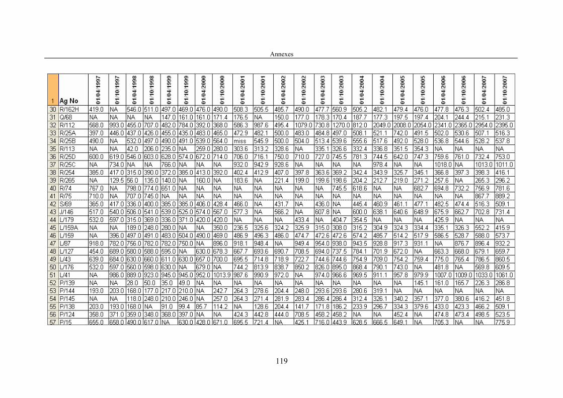
Annexes
119

Annexes
120
ANNEX 3 : Recharge rate (mm/m2/month) for all study wells from 1997 to 2006
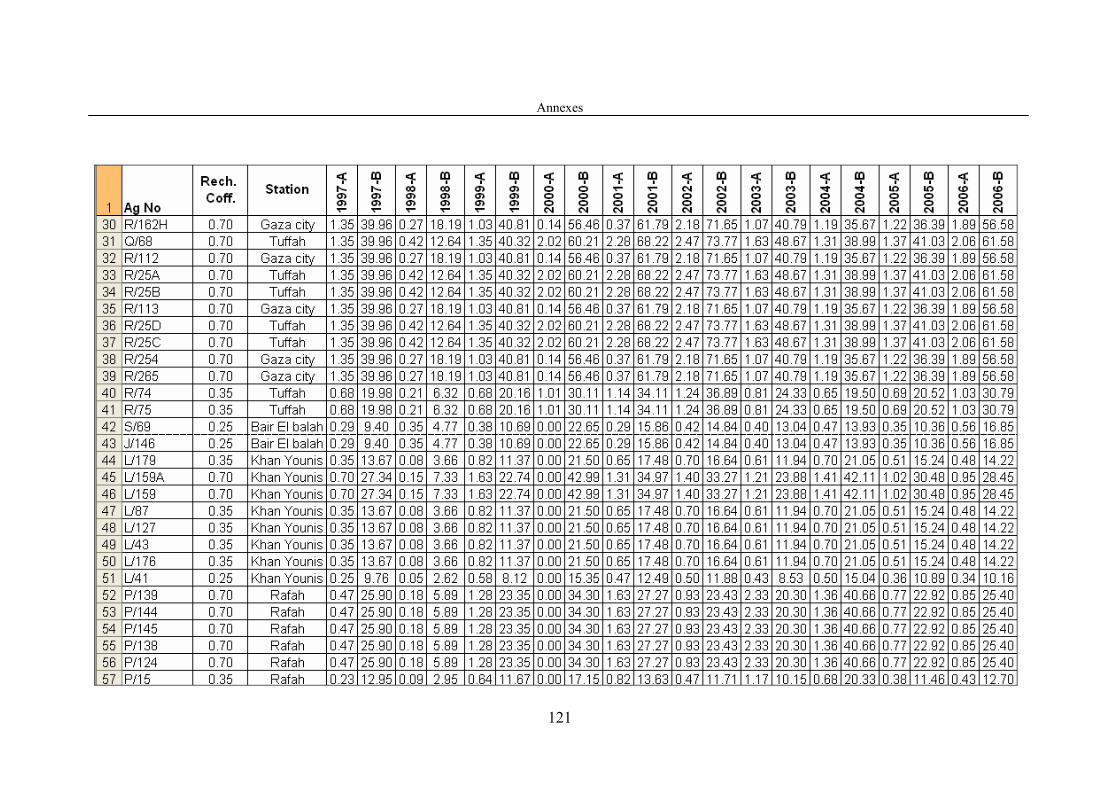
Annexes
121

Annexes
122
ANNEX 4: Abstraction hourly rate (m3/hour) for all study wells from 1997 to 2003

Annexes
123

Annexes
124
ANNEX 5 : Abstraction average rate (mm/m2/month) for areas of study wells from 1997 to 2006

Annexes
125

Annexes
126
ANNEX 6 : Data matrix of ANN model
Time phase
Well Clo R Q Qr Ot Wl Dw Th Ds Clf Clf-
predicted
1997-A D/67 78.0 2.14 48.23 18.71 20 -2 79 80 2.4 55.0 95.7
1997-A E/61 66.0 1.93 34.06 18.71 23 -1 43 40 1.3 145.0 120.1
1997-A A/185 70.0 1.93 172.86 18.71 14 -2 80 95 3.6 100.0 61.2
1997-A C/127 92.0 1.93 61.36 18.71 32 0 75 115 5.6 100.0 85.9
1997-A D/74 56.0 1.93 139.37 18.71 0 -2 81 50 2.0 65.0 74.9
1997-A D/68 92.0 1.93 177.38 18.71 9 -2 72 58 2.6 122.0 101.6
1997-A D/60 142.0 1.93 56.81 18.71 38 -2 45 43 3.3 129.0 183.4
1997-A C/79 427.0 0.96 0.00 18.71 27 0 64 90 6.4 384.0 438.6
1997-A E/4 108.0 1.93 81.63 18.71 37 -1 34 124 4.7 100.0 94.4
1997-A E/154 189.0 1.93 180.31 28.48 22 -2 92 50 1.7 180.0 222.3
1997-A C/128 234.0 0.96 118.65 18.71 13 1 110 86 7.7 259.0 221.2
1997-A E/157 142.0 1.93 198.43 18.71 11 -2 38 58 2.6 158.0 145.8
1997-A E/156 135.0 1.93 151.75 18.71 17 -1 70 80 4.2 135.0 131.9
1997-A E/90 142.0 1.93 74.01 18.71 27 -1 70 50 3.6 158.0 172.1
1997-A R/162B 1295.0 1.42 188.15 28.48 31 -1 70 30 1.7 1505.0 1472.7
1997-A R/162LA 262.0 1.35 126.23 28.48 11 -1 56 30 1.6 273.0 290.0
1997-A R/162G 440.0 1.93 196.53 28.48 33 -1 90 70 2.3 489.0 476.4
1997-A R/25A 397.0 1.35 116.88 28.48 17 -1 85 109 4.4 446.0 379.8
1997-A R/25D 600.0 1.35 181.30 28.48 25 -1 50 109 4.5 619.0 627.0
1997-A R/254 385.0 1.35 117.92 28.48 12 1 46 36 1.4 417.0 409.5
1997-A S/69 365.0 0.29 96.78 16.36 15 -1 73 71 5.1 417.0 375.3
1997-A J/146 517.0 0.29 95.09 16.36 13 -1 62 78 4.8 540.0 549.6
1997-A L/179 532.0 0.35 63.56 14.03 11 0 86 35 3.0 597.0 551.0
1997-A L/87 918.0 0.35 80.67 14.03 47 0 82 45 3.4 782.0 887.3
1997-A L/127 454.0 0.35 45.09 14.03 30 0 60 30 3.4 689.0 449.5
1997-A L/43 639.0 0.35 61.24 14.03 36 -1 79 69 3.9 684.0 656.1
1997-A L/176 532.0 0.35 149.77 14.03 14 -1 110 50 3.4 597.0 566.9
1997-A P/144 193.0 0.47 108.24 12.16 5 -3 80 30 2.8 203.0 205.7
1997-A P/138 203.0 0.47 3.60 12.16 17 -4 67 33 3.6 193.0 237.9
1997-A P/124 358.0 0.47 166.19 12.16 24 -3 48 42 3.1 371.0 355.7
1997-A P/15 655.0 0.23 130.46 12.16 29 -3 18 34 3.6 658.0 652.6
1997-B D/67 55.0 42.35 27.66 16.15 20 -2 79 80 2.4 56.0 71.9
1997-B E/61 145.0 49.18 30.42 16.15 23 -1 43 40 1.3 42.0 144.6
1997-B A/185 100.0 49.18 150.89 16.15 14 -2 80 95 3.6 77.0 81.0
1997-B C/127 100.0 49.18 34.87 16.15 32 0 75 115 5.6 70.0 96.1
1997-B D/74 65.0 49.18 142.48 16.15 0 -2 81 50 2.0 56.0 64.3
1997-B D/68 122.0 49.18 172.71 16.15 9 -2 72 58 2.6 112.0 105.3
1997-B D/60 129.0 49.18 55.78 16.15 38 -2 45 43 3.3 129.0 138.5
1997-B E/4 100.0 49.18 76.91 16.15 37 -1 34 124 4.7 84.0 91.7
1997-B E/154 180.0 49.18 186.47 24.39 22 -2 92 50 1.7 178.0 186.1
1997-B C/128 259.0 24.59 92.84 16.15 13 1 110 86 7.7 217.0 239.1
1997-B E/157 158.0 49.18 191.25 16.15 11 -2 38 58 2.6 136.0 133.8
1997-B E/90 158.0 49.18 94.07 16.15 27 -1 70 50 3.6 105.0 148.8
1997-B R/162B 504.0 32.84 21.17 24.39 31 -1 70 30 1.7 530.0 487.5
1997-B C/76 420.0 24.59 0.00 16.15 54 0 38 90 6.5 420.0 418.4
1997-B R/162L 312.0 39.96 178.43 24.39 27 -1 110 45 1.7 300.0 311.1
1997-B R/162LA 273.0 39.96 131.76 24.39 11 -1 56 30 1.6 287.0 267.8
1997-B R/162G 489.0 49.18 194.06 24.39 33 -1 90 70 2.3 441.0 491.6

Annexes
127
Time phase
Well Clo R Q Qr Ot Wl Dw Th Ds Clf Clf-
predicted
1997-B R/25A 446.0 39.96 154.96 24.39 17 -1 85 109 4.4 437.0 449.0
1997-B R/25D 619.0 39.96 153.48 24.39 25 -1 50 109 4.5 546.0 639.4
1997-B R/254 417.0 39.96 106.78 24.39 12 1 46 36 1.4 315.0 405.9
1997-B R/265 129.5 39.96 0.00 24.39 2 1 39 40 1.0 56.0 146.2
1997-B S/69 417.0 9.40 92.01 12.43 15 -1 73 71 5.1 336.0 417.8
1997-B J/146 540.0 9.40 40.88 12.43 13 -1 62 78 4.8 506.0 555.6
1997-B L/159 396.0 27.34 64.75 13.35 24 0 42 40 2.4 497.0 365.1
1997-B L/87 782.0 13.67 79.61 13.35 47 0 82 45 3.4 756.0 735.0
1997-B L/127 689.0 13.67 34.78 13.35 30 0 60 30 3.4 580.0 642.9
1997-B L/43 684.0 13.67 60.97 13.35 36 -1 79 69 3.9 630.0 683.7
1997-B L/176 597.0 13.67 108.47 13.35 14 -1 110 50 3.4 560.0 612.8
1997-B L/41 986.0 9.76 32.55 13.35 41 0 54 60 5.1 889.0 954.0
1997-B P/144 203.0 25.90 121.13 11.37 5 -3 80 30 2.8 168.0 185.4
1997-B P/138 193.0 25.90 12.24 11.37 17 -4 67 33 3.6 168.0 195.5
1997-B P/124 371.0 25.90 136.22 11.37 24 -3 48 42 3.1 359.0 335.2
1997-B P/15 658.0 12.95 0.15 11.37 29 -3 18 34 3.6 490.0 597.6
1998-A D/67 56.0 0.53 63.76 19.68 21 -2 79 80 2.4 56.0 77.7
1998-A A/180 49.0 0.53 28.58 19.68 16 -2 82 90 3.1 56.0 62.9
1998-A D/73 56.0 0.53 50.45 19.68 2 -2 79 53 2.1 63.0 85.9
1998-A E/61 42.0 0.44 28.58 19.68 24 -1 43 40 1.3 135.0 103.8
1998-A A/185 77.0 0.44 124.94 19.68 15 -2 80 95 3.6 85.0 71.3
1998-A D/71 70.0 0.44 149.70 19.68 0 -2 50 43 2.7 78.0 91.7
1998-A C/127 70.0 0.58 64.11 19.68 33 0 75 115 5.6 70.0 69.6
1998-A D/74 56.0 0.44 162.24 19.68 1 -2 81 50 2.0 71.0 75.4
1998-A D/70 70.0 0.44 168.94 19.68 2 -2 42 40 3.0 85.0 93.3
1998-A D/69 78.0 0.44 175.51 19.68 5 -2 40 58 2.7 78.0 89.4
1998-A E/6 56.0 0.44 7.52 19.68 36 -1 31 100 4.6 85.0 80.7
1998-A E/142 77.0 0.44 53.47 19.68 0 -3 37 52 2.1 100.0 101.2
1998-A D/68 112.0 0.44 172.64 19.68 10 -2 72 58 2.6 120.0 121.8
1998-A D/60 129.0 0.44 54.81 19.68 39 -2 45 43 3.3 121.0 174.7
1998-A E/4 84.0 0.44 121.02 19.68 38 -1 34 124 4.7 78.0 74.9
1998-A E/154 178.0 0.44 157.06 30.95 23 -2 92 50 1.7 230.0 215.4
1998-A C/128 217.0 0.29 138.27 19.68 14 1 110 86 7.7 235.0 205.5
1998-A E/157 136.0 0.44 182.99 19.68 12 -2 38 58 2.6 156.0 144.1
1998-A R/162B 530.0 0.23 31.23 30.95 32 -1 70 30 1.7 497.0 541.1
1998-A C/76 420.0 0.29 46.01 19.68 55 0 38 90 6.5 470.0 442.2
1998-A R/162L 300.0 0.27 206.95 30.95 28 -1 110 45 1.7 319.0 339.3
1998-A R/162LA 287.0 0.27 206.95 30.95 12 -1 56 30 1.6 284.0 329.6
1998-A R/162G 441.0 0.44 187.88 30.95 34 -1 90 70 2.3 461.0 474.2
1998-A R/162HA 458.0 0.27 195.39 30.95 8 -1 85 69 2.4 483.0 491.1
1998-A R/162H 546.0 0.27 149.87 30.95 25 -1 90 69 2.4 511.0 573.8
1998-A R/25A 437.0 0.42 149.51 30.95 18 -1 85 109 4.4 426.0 429.9
1998-A R/25B 532.0 0.42 192.39 30.95 48 -1 52 109 4.5 497.0 553.3
1998-A R/113 42.0 0.27 52.17 30.95 33 1 32 40 0.8 206.0 101.4
1998-A R/25D 546.0 0.42 129.32 30.95 26 -1 50 109 4.5 603.0 542.2
1998-A R/254 315.0 0.27 97.52 30.95 13 1 46 36 1.4 390.0 338.0
1998-A R/265 56.0 0.27 73.42 30.95 3 1 39 40 1.0 135.0 107.8
1998-A R/74 798.0 0.21 25.21 30.95 6 0 45 100 5.0 774.0 765.7
1998-A R/75 707.0 0.21 82.67 30.95 8 0 62 100 5.0 745.0 693.4

Annexes
128
Time phase
Well Clo R Q Qr Ot Wl Dw Th Ds Clf Clf-
predicted
1998-A S/69 336.0 0.35 92.18 18.76 16 -1 73 71 5.1 400.0 345.1
1998-A J/146 506.0 0.35 111.06 18.76 14 -1 62 78 4.8 541.0 538.2
1998-A L/179 315.0 0.08 57.53 19.20 12 0 86 35 3.0 369.0 337.9
1998-A L/159A 189.0 0.15 57.82 19.20 0 0 62 30 2.5 248.0 215.2
1998-A L/159 497.0 0.15 53.53 19.20 25 0 42 40 2.4 491.0 519.4
1998-A L/87 756.0 0.08 64.32 19.20 48 0 82 45 3.4 782.0 758.1
1998-A L/127 580.0 0.08 59.26 19.20 31 0 60 30 3.4 588.0 593.8
1998-A L/43 630.0 0.08 69.84 19.20 37 -1 79 69 3.9 660.0 663.8
1998-A L/176 560.0 0.08 138.78 19.20 15 -1 110 50 3.4 598.0 608.4
1998-A L/41 889.0 0.05 35.93 19.20 42 0 54 60 5.1 923.0 901.9
1998-A P/139 28.0 0.18 27.98 19.20 0 -1 30 30 0.8 50.0 86.5
1998-A P/144 168.0 0.18 100.50 12.67 6 -3 80 30 2.8 177.0 186.3
1998-A P/145 118.0 0.18 63.60 12.67 2 -4 75 40 4.0 248.0 143.6
1998-A P/124 359.0 0.18 115.56 12.67 25 -3 48 42 3.1 348.0 360.0
1998-A P/15 490.0 0.09 100.19 12.67 30 -3 18 34 3.6 617.0 480.2
1998-B D/67 56.0 17.48 57.74 17.00 21 -2 79 80 2.4 42.0 76.3
1998-B A/180 56.0 17.48 8.15 17.00 16 -2 82 90 3.1 49.0 71.8
1998-B D/73 63.0 17.48 53.36 17.00 2 -2 79 53 2.1 63.0 85.2
1998-B D/72 71.0 13.04 65.44 17.00 0 -2 46 41 2.9 77.0 97.7
1998-B E/61 135.0 13.04 8.15 17.00 24 -1 43 40 1.3 182.0 172.1
1998-B A/185 85.0 13.04 83.74 17.00 15 -2 80 95 3.6 84.0 79.5
1998-B D/71 78.0 13.04 126.59 17.00 0 -2 50 43 2.7 74.0 93.2
1998-B C/127 70.0 18.14 52.16 17.00 33 0 75 115 5.6 77.0 73.9
1998-B D/74 71.0 13.04 150.84 17.00 1 -2 81 50 2.0 77.0 81.5
1998-B D/70 85.0 13.04 170.89 17.00 2 -2 42 40 3.0 88.0 96.9
1998-B D/69 78.0 13.04 171.86 17.00 5 -2 40 58 2.7 70.0 82.9
1998-B E/6 85.0 13.04 5.21 17.00 36 -1 31 100 4.6 77.0 105.8
1998-B E/142 100.0 13.04 49.38 17.00 0 -3 37 52 2.1 112.0 115.7
1998-B D/68 120.0 13.04 159.30 17.00 10 -2 72 58 2.6 98.0 121.7
1998-B D/60 121.0 13.04 44.67 17.00 39 -2 45 43 3.3 119.0 160.3
1998-B E/4 78.0 13.04 109.49 17.00 38 -1 34 124 4.7 70.0 71.8
1998-B E/154 230.0 13.04 178.48 27.27 23 -2 92 50 1.7 266.0 256.0
1998-B C/128 235.0 9.07 99.71 17.00 14 1 110 86 7.7 217.0 221.8
1998-B E/157 156.0 13.04 147.20 17.00 12 -2 38 58 2.6 161.0 155.5
1998-B E/156 121.0 13.04 133.13 17.00 18 -1 70 80 4.2 140.0 118.2
1998-B R/162B 497.0 16.31 0.00 27.27 32 -1 70 30 1.7 491.0 496.8
1998-B C/76 470.0 9.07 4.56 17.00 55 0 38 90 6.5 448.0 479.9
1998-B R/162L 319.0 18.19 152.31 27.27 28 -1 110 45 1.7 272.0 338.1
1998-B R/162LA 284.0 18.19 77.75 27.27 12 -1 56 30 1.6 224.0 297.8
1998-B R/162G 461.0 13.04 141.08 27.27 34 -1 90 70 2.3 435.0 485.5
1998-B R/162HA 483.0 18.19 185.40 27.27 8 -1 85 69 2.4 462.0 512.0
1998-B R/162H 511.0 18.19 163.99 27.27 25 -1 90 69 2.4 497.0 538.4
1998-B R/112 707.0 18.19 52.47 27.27 33 1 36 30 0.6 482.0 711.8
1998-B R/25A 426.0 12.64 51.36 27.27 18 -1 85 109 4.4 455.0 405.8
1998-B R/25B 497.0 12.64 138.94 27.27 48 -1 52 109 4.5 490.0 517.2
1998-B R/113 206.0 18.19 141.07 27.27 33 1 32 40 0.8 235.0 232.4
1998-B R/25D 603.0 12.64 103.42 27.27 26 -1 50 109 4.5 628.0 613.4
1998-B R/254 390.0 18.19 58.12 27.27 13 1 46 36 1.4 372.0 397.0
1998-B R/265 135.0 18.19 108.41 27.27 3 1 39 40 1.0 140.0 164.2

Annexes
129
Time phase
Well Clo R Q Qr Ot Wl Dw Th Ds Clf Clf-
predicted
1998-B R/74 774.0 6.32 15.68 27.27 6 0 45 100 5.0 651.0 765.2
1998-B S/69 400.0 4.77 77.88 16.53 16 -1 73 71 5.1 385.0 411.4
1998-B J/146 541.0 4.77 106.32 16.53 14 -1 62 78 4.8 539.0 576.5
1998-B L/179 369.0 3.66 44.19 16.13 12 0 86 35 3.0 336.0 384.8
1998-B L/159A 248.0 7.33 53.31 16.13 0 0 62 30 2.5 280.0 262.8
1998-B L/159 491.0 7.33 47.51 16.13 25 0 42 40 2.4 483.0 494.8
1998-B L/87 782.0 3.66 85.88 16.13 48 0 82 45 3.4 782.0 769.4
1998-B L/127 588.0 3.66 65.40 16.13 31 0 60 30 3.4 595.0 583.7
1998-B L/43 660.0 3.66 60.81 16.13 37 -1 79 69 3.9 611.0 681.8
1998-B L/176 598.0 3.66 108.77 16.13 15 -1 110 50 3.4 630.0 636.9
1998-B L/41 923.0 2.62 35.93 16.13 42 0 54 60 5.1 945.0 918.3
1998-B P/139 50.0 5.89 5.86 16.13 0 -1 30 30 0.8 35.0 106.4
1998-B P/144 177.0 5.89 161.97 11.83 6 -3 80 30 2.8 217.0 177.7
1998-B P/145 248.0 5.89 98.27 11.83 2 -4 75 40 4.0 210.0 247.7
1998-B P/124 348.0 5.89 117.74 11.83 25 -3 48 42 3.1 368.0 338.4
1999-A A/180 49.0 2.22 5.56 20.65 17 -2 82 90 3.1 63.0 67.0
1999-A D/73 63.0 2.22 102.76 20.65 3 -2 79 53 2.1 63.0 86.4
1999-A A/185 84.0 1.47 132.13 20.65 16 -2 80 95 3.6 77.0 80.0
1999-A D/71 74.0 1.47 102.79 20.65 1 -2 50 43 2.7 66.0 101.0
1999-A C/127 77.0 1.52 60.84 20.65 34 0 75 115 5.6 84.0 77.3
1999-A D/74 77.0 1.47 196.21 20.65 2 -2 81 50 2.0 77.0 93.4
1999-A D/69 70.0 1.47 171.94 20.65 6 -2 40 58 2.7 70.0 86.1
1999-A E/6 77.0 1.47 10.87 20.65 37 -1 31 100 4.6 70.0 97.2
1999-A E/142 112.0 1.47 16.35 20.65 1 -3 37 52 2.1 105.0 135.9
1999-A D/68 98.0 1.47 141.80 20.65 11 -2 72 58 2.6 119.0 114.1
1999-A D/60 119.0 1.47 75.13 20.65 40 -2 45 43 3.3 105.0 164.0
1999-A C/79 427.0 0.76 4.57 20.65 29 0 64 90 6.4 463.7 436.8
1999-A E/4 70.0 1.47 94.34 20.65 39 -1 34 124 4.7 70.0 67.8
1999-A E/154 266.0 1.47 167.99 31.67 24 -2 92 50 1.7 190.0 300.3
1999-A C/128 217.0 0.76 120.01 20.65 15 1 110 86 7.7 224.0 207.9
1999-A E/157 161.0 1.47 176.99 20.65 13 -2 38 58 2.6 159.0 170.1
1999-A E/90 147.0 1.47 195.00 20.65 29 -1 70 50 3.6 154.0 169.6
1999-A R/162B 491.0 0.88 30.34 31.67 33 -1 70 30 1.7 490.0 501.4
1999-A R/162L 272.0 1.03 193.38 31.67 29 -1 110 45 1.7 300.0 311.1
1999-A R/162LA 224.0 1.03 125.66 31.67 13 -1 56 30 1.6 315.0 259.2
1999-A R/162G 435.0 1.47 172.83 31.67 35 -1 90 70 2.3 469.0 464.4
1999-A R/162H 497.0 1.03 175.57 31.67 26 -1 90 69 2.4 469.0 527.6
1999-A Q/68 147.0 1.35 42.97 20.65 0 -1 73 104 5.0 161.0 106.0
1999-A R/25A 455.0 1.35 134.87 31.67 19 -1 85 109 4.4 435.0 444.5
1999-A R/25B 490.0 1.35 56.86 31.67 49 -1 52 109 4.5 491.0 478.4
1999-A R/25D 628.0 1.35 90.20 31.67 27 -1 50 109 4.5 574.0 612.2
1999-A R/254 372.0 1.03 61.23 31.67 14 1 46 36 1.4 385.0 387.0
1999-A S/69 385.0 0.38 67.25 19.06 17 -1 73 71 5.1 385.0 399.2
1999-A J/146 539.0 0.38 94.09 19.06 15 -1 62 78 4.8 525.0 574.3
1999-A L/179 336.0 0.82 51.77 18.16 13 0 86 35 3.0 371.0 357.8
1999-A L/159 483.0 1.63 49.32 18.16 26 0 42 40 2.4 504.0 500.4
1999-A L/87 782.0 0.82 24.31 18.16 49 0 82 45 3.4 750.0 759.1
1999-A L/43 611.0 0.82 60.43 18.16 38 -1 79 69 3.9 630.0 638.5
1999-A L/41 945.0 0.58 64.47 18.16 43 0 54 60 5.1 945.0 967.4

Annexes
130
Time phase
Well Clo R Q Qr Ot Wl Dw Th Ds Clf Clf-
predicted
1999-A P/139 35.0 1.28 6.46 18.16 1 -1 30 30 0.8 49.0 97.2
1999-A P/144 217.0 1.28 164.83 14.08 7 -3 80 30 2.8 210.0 222.6
1999-A P/145 210.0 1.28 98.45 14.08 3 -4 75 40 4.0 246.0 219.5
1999-A P/138 91.0 1.28 59.48 14.08 19 -4 67 33 3.6 99.4 135.9
1999-A P/124 368.0 1.28 151.81 14.08 26 -3 48 42 3.1 397.0 372.5
1999-B A/180 63.0 48.11 5.56 18.32 17 -2 82 90 3.1 70.0 75.5
1999-B D/73 63.0 48.11 68.30 18.32 3 -2 79 53 2.1 63.0 74.3
1999-B A/185 77.0 43.86 116.28 18.32 16 -2 80 95 3.6 91.3 75.3
1999-B D/71 66.0 43.86 193.38 18.32 1 -2 50 43 2.7 77.0 72.8
1999-B C/127 84.0 46.16 43.95 18.32 34 0 75 115 5.6 77.0 89.7
1999-B D/74 77.0 43.86 191.38 18.32 2 -2 81 50 2.0 77.0 79.1
1999-B D/69 70.0 43.86 173.28 18.32 6 -2 40 58 2.7 98.0 74.0
1999-B E/6 70.0 43.86 6.22 18.32 37 -1 31 100 4.6 84.0 91.5
1999-B D/68 119.0 43.86 178.39 18.32 11 -2 72 58 2.6 91.0 112.5
1999-B C/79 463.7 23.08 38.59 18.32 29 0 64 90 6.4 483.0 467.5
1999-B E/4 70.0 43.86 85.69 18.32 39 -1 34 124 4.7 77.0 75.8
1999-B E/154 190.0 43.86 175.27 27.75 24 -2 92 50 1.7 322.0 210.3
1999-B C/128 224.0 23.08 72.59 18.32 15 1 110 86 7.7 231.0 211.8
1999-B E/157 159.0 43.86 174.57 18.32 13 -2 38 58 2.6 182.0 145.7
1999-B E/90 154.0 43.86 183.02 18.32 29 -1 70 50 3.6 168.0 150.2
1999-B R/162L 300.0 40.81 191.77 27.75 29 -1 110 45 1.7 413.0 309.7
1999-B R/162G 469.0 43.86 164.50 27.75 35 -1 90 70 2.3 490.0 475.2
1999-B R/162H 469.0 40.81 105.87 27.75 26 -1 90 69 2.4 476.0 470.0
1999-B Q/68 161.0 40.32 169.74 18.32 0 -1 73 104 5.0 161.0 129.1
1999-B R/25A 435.0 40.32 135.42 27.75 19 -1 85 109 4.4 483.0 440.2
1999-B R/25B 491.0 40.32 79.80 27.75 49 -1 52 109 4.5 539.0 494.1
1999-B R/25D 574.0 40.32 147.94 27.75 27 -1 50 109 4.5 672.0 582.8
1999-B R/254 385.0 40.81 90.55 27.75 14 1 46 36 1.4 413.0 378.4
1999-B S/69 385.0 10.69 81.13 17.89 17 -1 73 71 5.1 406.0 391.7
1999-B J/146 525.0 10.69 107.43 17.89 15 -1 62 78 4.8 574.0 552.5
1999-B L/179 371.0 11.37 51.97 17.48 13 0 86 35 3.0 420.0 377.7
1999-B L/159 504.0 22.74 54.34 17.48 26 0 42 40 2.4 490.0 492.1
1999-B L/43 630.0 11.37 66.25 17.48 38 -1 79 69 3.9 657.0 647.8
1999-B L/41 945.0 8.12 61.48 17.48 43 0 54 60 5.1 952.0 956.0
1999-B P/138 99.4 23.35 27.59 12.77 19 -4 67 33 3.6 85.7 130.0
1999-B P/15 630.0 11.67 69.51 12.77 31 -3 18 34 3.6 428.0 595.6
2000-A D/67 42.0 0.12 33.11 22.32 23 -2 79 80 2.4 35.3 72.6
2000-A A/180 70.0 0.12 14.56 22.32 18 -2 82 90 3.1 77.0 82.1
2000-A D/73 63.0 0.12 102.25 22.32 4 -2 79 53 2.1 56.0 89.5
2000-A D/72 70.0 2.04 173.83 22.32 2 -2 46 41 2.9 63.0 98.1
2000-A A/185 91.3 2.04 111.46 22.32 17 -2 80 95 3.6 91.0 90.9
2000-A D/71 77.0 2.04 201.56 22.32 2 -2 50 43 2.7 70.0 102.1
2000-A C/127 77.0 0.00 62.57 22.32 35 0 75 115 5.6 77.0 78.7
2000-A D/74 77.0 2.04 155.89 22.32 3 -2 81 50 2.0 77.0 99.5
2000-A D/70 91.0 2.04 158.07 22.32 4 -2 42 40 3.0 91.0 117.2
2000-A D/69 98.0 2.04 168.69 22.32 7 -2 40 58 2.7 91.0 114.2
2000-A E/6 84.0 2.04 84.86 22.32 38 -1 31 100 4.6 91.0 99.8
2000-A D/68 91.0 2.04 188.65 22.32 12 -2 72 58 2.6 126.0 110.9
2000-A C/79 483.0 0.00 39.24 22.32 30 0 64 90 6.4 478.0 497.5

Annexes
131
Time phase
Well Clo R Q Qr Ot Wl Dw Th Ds Clf Clf-
predicted
2000-A E/4 77.0 2.04 78.89 22.32 40 -1 34 124 4.7 77.0 76.7
2000-A E/154 322.0 2.04 174.27 32.24 25 -2 92 50 1.7 371.2 356.1
2000-A C/128 231.0 0.00 101.76 22.32 16 1 110 86 7.7 245.0 224.0
2000-A E/157 182.0 2.04 167.82 22.32 14 -2 38 58 2.6 175.0 194.3
2000-A E/156 140.0 2.04 159.69 22.32 20 -1 70 80 4.2 161.0 146.3
2000-A E/90 168.0 2.04 175.07 22.32 30 -1 70 50 3.6 175.0 192.9
2000-A C/76 525.0 0.00 19.54 22.32 57 0 38 90 6.5 532.0 544.3
2000-A R/162G 490.0 2.04 152.97 32.24 36 -1 90 70 2.3 514.0 514.8
2000-A R/162H 476.0 0.14 134.68 32.24 27 -1 90 69 2.4 490.0 495.4
2000-A Q/68 161.0 2.02 209.71 22.32 1 -1 73 104 5.0 171.4 133.3
2000-A R/112 392.0 0.14 60.01 32.24 35 1 36 30 0.6 368.0 410.2
2000-A R/25A 483.0 2.02 126.27 32.24 20 -1 85 109 4.4 465.0 470.4
2000-A R/25B 539.0 2.02 183.94 32.24 50 -1 52 109 4.5 564.0 554.7
2000-A R/113 259.0 0.14 76.55 32.24 35 1 32 40 0.8 280.0 285.0
2000-A R/25D 672.0 2.02 155.85 32.24 28 -1 50 109 4.5 714.0 678.4
2000-A R/254 413.0 0.14 116.30 32.24 15 1 46 36 1.4 392.0 436.6
2000-A S/69 406.0 0.00 75.49 21.17 18 -1 73 71 5.1 428.4 422.2
2000-A J/146 574.0 0.00 109.91 21.17 16 -1 62 78 4.8 567.0 616.3
2000-A L/179 420.0 0.00 65.82 20.23 14 0 86 35 3.0 420.0 444.8
2000-A L/159 490.0 0.00 57.96 20.23 27 0 42 40 2.4 469.0 513.4
2000-A L/127 630.0 0.00 79.55 20.23 33 0 60 30 3.4 678.3 649.6
2000-A L/43 657.0 0.00 66.25 20.23 39 -1 79 69 3.9 700.0 690.9
2000-A L/41 952.0 0.00 76.32 20.23 44 0 54 60 5.1 1013.9 988.0
2000-A P/138 85.7 0.00 50.10 14.85 20 -4 67 33 3.6 114.2 135.7
2000-A P/15 428.0 0.00 90.29 14.85 32 -3 18 34 3.6 671.0 430.3
2000-B D/67 35.3 55.46 30.00 19.63 23 -2 79 80 2.4 35.5 61.8
2000-B A/180 77.0 55.46 43.37 19.63 18 -2 82 90 3.1 84.0 84.5
2000-B D/73 56.0 55.46 73.93 19.63 4 -2 79 53 2.1 70.6 69.9
2000-B D/72 63.0 60.96 166.51 19.63 2 -2 46 41 2.9 63.5 71.0
2000-B A/185 91.0 60.96 112.72 19.63 17 -2 80 95 3.6 84.7 89.0
2000-B D/71 70.0 60.96 184.56 19.63 2 -2 50 43 2.7 77.7 75.2
2000-B C/127 77.0 56.00 42.50 19.63 35 0 75 115 5.6 77.7 87.7
2000-B D/74 77.0 60.96 101.11 19.63 3 -2 81 50 2.0 76.5 80.9
2000-B D/70 91.0 60.96 152.29 19.63 4 -2 42 40 3.0 98.8 90.8
2000-B D/69 91.0 60.96 181.04 19.63 7 -2 40 58 2.7 98.8 89.0
2000-B E/6 91.0 60.96 81.90 19.63 38 -1 31 100 4.6 98.8 100.6
2000-B D/68 126.0 60.96 174.68 19.63 12 -2 72 58 2.6 127.1 116.2
2000-B C/79 478.0 28.00 13.95 19.63 30 0 64 90 6.4 473.0 477.9
2000-B E/4 77.0 60.96 32.85 19.63 40 -1 34 124 4.7 69.5 88.1
2000-B E/154 371.2 60.96 140.29 28.22 25 -2 92 50 1.7 466.0 360.0
2000-B C/128 245.0 28.00 82.65 19.63 16 1 110 86 7.7 247.1 233.4
2000-B E/157 175.0 60.96 139.73 19.63 14 -2 38 58 2.6 176.5 155.8
2000-B E/156 161.0 60.96 118.70 19.63 20 -1 70 80 4.2 153.0 146.4
2000-B E/90 175.0 60.96 130.65 19.63 30 -1 70 50 3.6 139.1 163.3
2000-B C/76 532.0 28.00 10.89 19.63 57 0 38 90 6.5 578.9 533.0
2000-B R/162G 514.0 60.96 154.18 28.22 36 -1 90 70 2.3 515.4 504.2
2000-B R/162HA 490.0 56.46 93.99 28.22 10 -1 85 69 2.4 501.3 478.0
2000-B R/162H 490.0 56.46 132.42 28.22 27 -1 90 69 2.4 508.3 482.5
2000-B Q/68 171.4 60.21 199.26 19.63 1 -1 73 104 5.0 176.5 145.0

Annexes
132
Time phase
Well Clo R Q Qr Ot Wl Dw Th Ds Clf Clf-
predicted
2000-B R/25A 465.0 60.21 118.81 28.22 20 -1 85 109 4.4 472.9 460.6
2000-B R/113 280.0 56.46 73.24 28.22 35 1 32 40 0.8 303.6 274.3
2000-B R/25D 714.0 60.21 175.96 28.22 28 -1 50 109 4.5 706.0 708.7
2000-B R/254 392.0 56.46 72.83 28.22 15 1 46 36 1.4 402.4 371.5
2000-B S/69 428.4 22.65 53.77 19.25 18 -1 73 71 5.1 466.0 428.8
2000-B J/146 567.0 22.65 103.08 19.25 16 -1 62 78 4.8 577.3 590.3
2000-B L/159A 350.0 42.99 64.01 18.82 2 0 62 30 2.5 236.5 319.9
2000-B L/159 469.0 42.99 52.80 18.82 27 0 42 40 2.4 486.9 438.2
2000-B L/87 896.0 21.50 49.04 18.82 50 0 82 45 3.4 918.1 864.7
2000-B L/127 678.3 21.50 71.44 18.82 33 0 60 30 3.4 667.7 666.7
2000-B L/43 700.0 21.50 43.42 18.82 39 -1 79 69 3.9 695.5 707.4
2000-B L/41 1013.9 15.35 70.86 18.82 44 0 54 60 5.1 987.6 1032.3
2000-B P/144 242.7 34.30 128.28 13.71 8 -3 80 30 2.8 264.3 216.0
2000-B P/145 257.0 34.30 0.00 13.71 4 -4 75 40 4.0 264.3 242.1
2000-B P/15 671.0 17.15 48.39 13.71 32 -3 18 34 3.6 695.5 629.2
2001-A D/67 35.5 0.58 48.20 23.99 24 -2 79 80 2.4 35.3 68.4
2001-A A/180 84.0 0.58 69.11 23.99 19 -2 82 90 3.1 92.2 93.0
2001-A D/73 70.6 0.58 103.72 23.99 5 -2 79 53 2.1 70.9 98.6
2001-A D/72 63.5 2.14 174.81 23.99 3 -2 46 41 2.9 85.1 97.9
2001-A E/61 1412.0 2.14 149.77 23.99 27 -1 43 40 1.3 1744.1 1576.6
2001-A A/185 84.7 2.14 144.95 23.99 18 -2 80 95 3.6 106.4 91.5
2001-A D/71 77.7 2.14 185.71 23.99 3 -2 50 43 2.7 92.2 108.3
2001-A C/127 77.7 0.58 68.88 23.99 36 0 75 115 5.6 77.9 82.1
2001-A D/74 76.5 2.14 166.44 23.99 4 -2 81 50 2.0 70.8 104.0
2001-A D/70 98.8 2.14 151.15 23.99 5 -2 42 40 3.0 99.3 128.1
2001-A D/69 98.8 2.14 170.48 23.99 8 -2 40 58 2.7 106.8 120.2
2001-A E/6 98.8 2.14 86.92 23.99 39 -1 31 100 4.6 99.3 114.2
2001-A D/68 127.1 2.14 177.29 23.99 13 -2 72 58 2.6 134.7 147.3
2001-A C/79 473.0 0.29 33.80 23.99 31 0 64 90 6.4 489.2 482.5
2001-A E/4 69.5 2.14 60.11 23.99 41 -1 34 124 4.7 77.9 73.7
2001-A E/154 466.0 2.14 149.18 32.81 26 -2 92 50 1.7 567.2 492.7
2001-A C/128 247.1 0.29 107.64 23.99 17 1 110 86 7.7 248.2 242.9
2001-A E/157 176.5 2.14 159.68 23.99 15 -2 38 58 2.6 170.2 193.1
2001-A E/156 153.0 2.14 163.91 23.99 21 -1 70 80 4.2 148.8 163.1
2001-A E/90 139.1 2.14 177.93 23.99 31 -1 70 50 3.6 177.2 170.2
2001-A R/162L 499.1 0.37 184.03 32.81 31 -1 110 45 1.7 494.2 534.7
2001-A R/162G 515.4 2.14 183.70 32.81 37 -1 90 70 2.3 526.8 545.6
2001-A R/162HA 501.3 0.37 85.40 32.81 11 -1 85 69 2.4 512.6 500.0
2001-A R/162H 508.3 0.37 139.84 32.81 28 -1 90 69 2.4 505.5 528.1
2001-A R/25A 472.9 2.28 121.43 32.81 21 -1 85 109 4.4 482.1 458.7
2001-A R/113 303.6 0.37 73.73 32.81 36 1 32 40 0.8 313.2 325.7
2001-A R/25D 706.0 2.28 193.60 32.81 29 -1 50 109 4.5 716.1 722.9
2001-A R/25C 932.0 2.28 48.99 32.81 44 -1 45 109 4.5 942.9 911.1
2001-A R/254 402.4 0.37 107.34 32.81 16 1 46 36 1.4 412.9 424.1
2001-A L/159A 236.5 1.31 71.20 22.29 3 0 62 30 2.5 325.6 258.9
2001-A L/159 486.9 1.31 58.94 22.29 28 0 42 40 2.4 496.3 510.5
2001-A L/87 918.1 0.65 64.78 22.29 51 0 82 45 3.4 948.4 924.6
2001-A L/127 667.7 0.65 95.31 22.29 34 0 60 30 3.4 693.6 696.6
2001-A L/43 695.5 0.65 70.12 22.29 40 -1 79 69 3.9 714.8 731.5

Annexes
133
Time phase
Well Clo R Q Qr Ot Wl Dw Th Ds Clf Clf-
predicted
2001-A L/176 744.2 0.65 139.84 22.29 18 -1 110 50 3.4 813.9 825.0
2001-A L/41 987.6 0.47 78.70 22.29 45 0 54 60 5.1 990.9 1029.4
2001-A P/144 264.3 1.63 126.24 15.61 9 -3 80 30 2.8 278.6 275.3
2001-A P/145 264.3 1.63 0.00 15.61 5 -4 75 40 4.0 271.4 292.0
2001-A P/124 424.3 1.63 176.74 15.61 28 -3 48 42 3.1 442.8 438.6
2001-A P/15 695.5 0.82 86.36 15.61 33 -3 18 34 3.6 721.4 698.2
2001-B D/67 35.3 62.13 31.39 20.95 24 -2 79 80 2.4 42.5 63.6
2001-B A/180 92.2 62.13 45.14 20.95 19 -2 82 90 3.1 106.1 98.5
2001-B D/73 70.9 62.13 84.23 20.95 5 -2 79 53 2.1 70.8 81.3
2001-B D/72 85.1 63.84 166.99 20.95 3 -2 46 41 2.9 85.7 90.0
2001-B A/185 106.4 63.84 131.04 20.95 18 -2 80 95 3.6 113.2 105.7
2001-B D/71 92.2 63.84 139.67 20.95 3 -2 50 43 2.7 100.0 94.7
2001-B C/127 77.9 62.29 60.65 20.95 36 0 75 115 5.6 92.0 91.5
2001-B D/74 70.8 63.84 131.79 20.95 4 -2 81 50 2.0 92.0 79.8
2001-B D/70 99.3 63.84 128.92 20.95 5 -2 42 40 3.0 107.1 100.3
2001-B D/69 106.8 63.84 145.33 20.95 8 -2 40 58 2.7 114.3 105.3
2001-B E/6 99.3 63.84 59.11 20.95 39 -1 31 100 4.6 106.1 111.5
2001-B D/68 134.7 63.84 182.67 20.95 13 -2 72 58 2.6 142.8 127.2
2001-B C/79 489.2 31.14 24.25 20.95 31 0 64 90 6.4 502.5 489.0
2001-B E/4 77.9 63.84 37.04 20.95 41 -1 34 124 4.7 70.8 92.8
2001-B C/128 248.2 31.14 91.95 20.95 17 1 110 86 7.7 261.8 239.0
2001-B E/157 170.2 63.84 165.42 20.95 15 -2 38 58 2.6 178.6 155.6
2001-B E/156 148.8 63.84 151.73 20.95 21 -1 70 80 4.2 184.6 140.3
2001-B R/162L 494.2 61.79 139.80 28.70 31 -1 110 45 1.7 521.4 476.4
2001-B R/162G 526.8 63.84 134.01 28.70 37 -1 90 70 2.3 542.0 512.6
2001-B R/162HA 512.6 61.79 95.73 28.70 11 -1 85 69 2.4 485.7 497.0
2001-B R/162H 505.5 61.79 125.31 28.70 28 -1 90 69 2.4 485.7 492.6
2001-B R/25A 482.1 68.22 117.71 28.70 21 -1 85 109 4.4 500.0 472.6
2001-B R/25B 545.9 68.22 144.20 28.70 51 -1 52 109 4.5 500.0 530.9
2001-B R/113 313.2 61.79 69.27 28.70 36 1 32 40 0.8 328.6 300.5
2001-B R/25D 716.1 68.22 188.49 28.70 29 -1 50 109 4.5 750.0 698.4
2001-B R/25C 942.9 68.22 1.34 28.70 44 -1 45 109 4.5 928.6 896.4
2001-B R/254 412.9 61.79 82.19 28.70 16 1 46 36 1.4 407.0 388.9
2001-B L/159A 325.6 34.97 73.38 20.17 3 0 62 30 2.5 324.2 308.8
2001-B L/159 496.3 34.97 52.10 20.17 28 0 42 40 2.4 486.0 477.9
2001-B L/127 693.6 17.48 87.59 20.17 34 0 60 30 3.4 690.7 697.1
2001-B L/43 714.8 17.48 58.35 20.17 40 -1 79 69 3.9 718.9 733.0
2001-B L/176 813.9 17.48 144.75 20.17 18 -1 110 50 3.4 838.7 895.8
2001-B L/41 990.9 12.49 75.61 20.17 45 0 54 60 5.1 972.0 1016.6
2001-B P/144 278.6 27.27 116.66 14.65 9 -3 80 30 2.8 204.4 258.6
2001-B P/145 271.4 27.27 0.00 14.65 5 -4 75 40 4.0 281.9 265.1
2001-B P/138 128.6 27.27 56.09 14.65 21 -4 67 33 3.6 204.4 145.0
2001-B P/124 442.8 27.27 181.50 14.65 28 -3 48 42 3.1 444.0 426.1
2002-A D/67 42.5 1.11 43.03 25.65 25 -2 79 80 2.4 35.5 75.6
2002-A A/180 106.1 1.11 63.72 25.65 20 -2 82 90 3.1 99.5 113.6
2002-A D/73 70.8 1.11 125.74 25.65 6 -2 79 53 2.1 64.0 102.7
2002-A D/72 85.7 2.62 172.84 25.65 4 -2 46 41 2.9 78.2 121.2
2002-A A/185 113.2 2.62 175.84 25.65 19 -2 80 95 3.6 106.0 123.5
2002-A D/71 100.0 2.62 200.22 25.65 4 -2 50 43 2.7 71.0 133.4

Annexes
134
Time phase
Well Clo R Q Qr Ot Wl Dw Th Ds Clf Clf-
predicted
2002-A D/74 92.0 2.62 175.08 25.65 5 -2 81 50 2.0 86.5 122.7
2002-A D/70 107.1 2.62 138.90 25.65 6 -2 42 40 3.0 78.1 139.3
2002-A D/69 114.3 2.62 170.52 25.65 9 -2 40 58 2.7 85.2 139.1
2002-A E/6 106.1 2.62 80.81 25.65 40 -1 31 100 4.6 85.0 122.5
2002-A D/68 142.8 2.62 191.37 25.65 14 -2 72 58 2.6 106.0 167.4
2002-A C/79 502.5 0.85 52.38 25.65 32 0 64 90 6.4 476.0 513.0
2002-A E/4 70.8 2.62 41.71 25.65 42 -1 34 124 4.7 77.9 76.9
2002-A E/154 235.7 2.62 131.76 33.38 27 -2 92 50 1.7 177.6 268.8
2002-A C/128 261.8 0.85 98.56 25.65 18 1 110 86 7.7 248.0 259.1
2002-A E/157 178.6 2.62 163.73 25.65 16 -2 38 58 2.6 127.9 199.6
2002-A E/156 184.6 2.62 196.08 25.65 22 -1 70 80 4.2 156.0 200.3
2002-A C/76 608.6 0.85 22.41 25.65 59 0 38 90 6.5 593.0 622.2
2002-A R/162L 521.4 2.18 166.89 33.38 32 -1 110 45 1.7 518.0 551.3
2002-A R/162LA 664.3 2.18 154.76 33.38 16 -1 56 30 1.6 710.0 701.8
2002-A R/162G 542.0 2.62 165.67 33.38 38 -1 90 70 2.3 782.0 566.7
2002-A R/162HA 485.7 2.18 178.59 33.38 12 -1 85 69 2.4 490.0 513.7
2002-A R/162H 485.7 2.18 130.73 33.38 29 -1 90 69 2.4 490.0 502.3
2002-A Q/68 150.0 2.47 231.34 25.65 3 -1 73 104 5.0 177.0 145.5
2002-A R/25A 500.0 2.47 126.53 33.38 22 -1 85 109 4.4 483.0 487.0
2002-A R/25B 500.0 2.47 155.76 33.38 52 -1 52 109 4.5 504.0 507.3
2002-A R/25D 750.0 2.47 208.94 33.38 30 -1 50 109 4.5 710.0 769.8
2002-A R/254 407.0 2.18 104.61 33.38 17 1 46 36 1.4 397.8 427.2
2002-A R/265 221.4 2.18 53.12 33.38 7 1 39 40 1.0 199.0 244.4
2002-A L/159A 324.2 1.40 76.99 24.36 4 0 62 30 2.5 325.9 345.2
2002-A L/159 486.0 1.40 51.99 24.36 29 0 42 40 2.4 474.7 508.8
2002-A L/127 690.7 0.70 88.53 24.36 35 0 60 30 3.4 708.5 720.6
2002-A L/43 718.9 0.70 73.17 24.36 41 -1 79 69 3.9 722.7 754.3
2002-A L/176 838.7 0.70 134.28 24.36 19 -1 110 50 3.4 850.2 931.4
2002-A P/144 204.4 0.93 142.40 16.38 10 -3 80 30 2.8 248.0 218.4
2002-A P/145 281.9 0.93 0.00 16.38 6 -4 75 40 4.0 283.4 309.9
2002-A P/138 204.4 0.93 62.91 16.38 22 -4 67 33 3.6 141.7 231.9
2002-A P/124 444.0 0.93 187.38 16.38 29 -3 48 42 3.1 708.5 464.8
2002-B D/67 35.5 83.07 30.90 22.27 25 -2 79 80 2.4 50.0 63.1
2002-B A/180 99.5 83.07 57.37 22.27 20 -2 82 90 3.1 99.5 103.9
2002-B D/73 64.0 83.07 95.90 22.27 6 -2 79 53 2.1 71.6 75.2
2002-B D/72 78.2 78.19 172.42 22.27 4 -2 46 41 2.9 78.4 86.5
2002-B A/185 106.0 78.19 141.74 22.27 19 -2 80 95 3.6 107.4 109.0
2002-B D/71 71.0 78.19 214.88 22.27 4 -2 50 43 2.7 85.5 82.8
2002-B D/70 78.1 78.19 126.16 22.27 6 -2 42 40 3.0 99.8 85.7
2002-B D/69 85.2 78.19 159.84 22.27 9 -2 40 58 2.7 99.8 91.7
2002-B E/6 85.0 78.19 61.63 22.27 40 -1 31 100 4.6 107.8 102.1
2002-B D/68 106.0 78.19 188.31 22.27 14 -2 72 58 2.6 142.6 107.0
2002-B C/79 476.0 46.05 17.52 22.27 32 0 64 90 6.4 479.7 465.0
2002-B E/4 77.9 78.19 44.45 22.27 42 -1 34 124 4.7 87.7 96.3
2002-B C/128 248.0 46.05 90.40 22.27 18 1 110 86 7.7 222.0 237.7
2002-B E/157 127.9 78.19 149.75 22.27 16 -2 38 58 2.6 189.3 122.7
2002-B E/156 156.0 78.19 179.72 22.27 22 -1 70 80 4.2 164.7 146.2
2002-B E/90 191.0 78.19 166.67 22.27 32 -1 70 50 3.6 200.5 175.7
2002-B C/76 593.0 46.05 16.68 22.27 59 0 38 90 6.5 615.8 585.9

Annexes
135
Time phase
Well Clo R Q Qr Ot Wl Dw Th Ds Clf Clf-
predicted
2002-B R/162L 518.0 71.65 153.33 29.17 32 -1 110 45 1.7 620.0 491.9
2002-B R/162LA 710.0 71.65 149.24 29.17 16 -1 56 30 1.6 710.0 695.4
2002-B R/162G 782.0 78.19 178.15 29.17 38 -1 90 70 2.3 542.0 755.0
2002-B R/162HA 490.0 71.65 151.82 29.17 12 -1 85 69 2.4 520.5 474.9
2002-B R/162H 490.0 71.65 131.97 29.17 29 -1 90 69 2.4 477.7 469.7
2002-B Q/68 177.0 73.77 199.14 22.27 3 -1 73 104 5.0 178.3 164.8
2002-B R/25A 483.0 73.77 120.69 29.17 22 -1 85 109 4.4 484.8 470.5
2002-B R/25B 504.0 73.77 129.37 29.17 52 -1 52 109 4.5 513.4 486.5
2002-B R/25D 710.0 73.77 182.87 29.17 30 -1 50 109 4.5 727.0 682.5
2002-B R/254 397.8 71.65 73.56 29.17 17 1 46 36 1.4 363.6 367.4
2002-B R/265 199.0 71.65 47.26 29.17 7 1 39 40 1.0 199.6 201.5
2002-B L/159A 325.9 33.27 95.22 21.51 4 0 62 30 2.5 315.0 314.0
2002-B L/159 474.7 33.27 65.87 21.51 29 0 42 40 2.4 472.6 462.7
2002-B L/87 949.4 16.64 69.03 21.51 52 0 82 45 3.4 954.0 942.9
2002-B L/127 708.5 16.64 80.62 21.51 35 0 60 30 3.4 694.0 715.0
2002-B L/43 722.7 16.64 70.59 21.51 41 -1 79 69 3.9 744.6 746.9
2002-B L/176 850.2 16.64 119.28 21.51 19 -1 110 50 3.4 826.0 926.4
2002-B P/144 248.0 23.43 103.73 15.59 10 -3 80 30 2.8 293.6 238.5
2002-B P/145 283.4 23.43 0.00 15.59 6 -4 75 40 4.0 286.4 282.3
2002-B P/138 141.7 23.43 59.61 15.59 22 -4 67 33 3.6 171.8 159.0
2003-A D/67 50.0 1.40 48.39 27.32 26 -2 79 80 2.4 42.6 83.2
2003-A A/180 99.5 1.40 83.71 27.32 21 -2 82 90 3.1 113.6 113.1
2003-A D/73 71.6 1.40 128.11 27.32 7 -2 79 53 2.1 63.9 108.3
2003-A A/185 107.4 1.41 246.55 27.32 20 -2 80 95 3.6 120.7 132.9
2003-A D/70 99.8 1.41 150.54 27.32 7 -2 42 40 3.0 106.5 138.1
2003-A D/69 99.8 1.41 188.73 27.32 10 -2 40 58 2.7 113.6 134.0
2003-A E/6 107.8 1.41 16.47 27.32 41 -1 31 100 4.6 114.1 121.8
2003-A D/68 142.6 1.41 208.75 27.32 15 -2 72 58 2.6 142.0 174.5
2003-A C/79 479.7 0.70 6.77 27.32 33 0 64 90 6.4 475.7 476.0
2003-A E/4 87.7 1.41 58.15 27.32 43 -1 34 124 4.7 92.3 91.9
2003-A E/154 841.0 1.41 154.59 33.94 28 -2 92 50 1.7 1036.6 883.7
2003-A C/128 222.0 0.70 103.49 27.32 19 1 110 86 7.7 255.6 223.1
2003-A E/157 189.3 1.41 176.15 27.32 17 -2 38 58 2.6 184.6 215.1
2003-A E/156 164.7 1.41 199.56 27.32 23 -1 70 80 4.2 156.2 187.3
2003-A E/90 200.5 1.41 179.28 27.32 33 -1 70 50 3.6 184.6 233.5
2003-A C/76 615.8 0.70 17.86 27.32 60 0 38 90 6.5 624.8 624.3
2003-A R/162L 620.0 1.07 186.49 33.94 33 -1 110 45 1.7 624.8 654.9
2003-A R/162LA 710.0 1.07 141.22 33.94 17 -1 56 30 1.6 823.6 744.6
2003-A R/162G 542.0 1.41 214.81 33.94 39 -1 90 70 2.3 553.8 575.6
2003-A R/162HA 520.5 1.07 205.72 33.94 13 -1 85 69 2.4 511.2 556.3
2003-A R/162H 477.7 1.07 157.41 33.94 30 -1 90 69 2.4 560.9 500.1
2003-A Q/68 178.3 1.63 254.94 27.32 4 -1 73 104 5.0 170.4 184.9
2003-A R/25A 484.8 1.63 130.61 33.94 23 -1 85 109 4.4 497.0 472.2
2003-A R/25B 513.4 1.63 198.60 33.94 53 -1 52 109 4.5 539.6 526.6
2003-A R/113 335.1 1.07 90.93 33.94 38 1 32 40 0.8 326.6 356.8
2003-A R/25D 727.0 1.63 213.99 33.94 31 -1 50 109 4.5 745.5 742.9
2003-A R/254 363.6 1.07 75.57 33.94 18 1 46 36 1.4 369.2 380.2
2003-A R/265 199.6 1.07 55.68 33.94 8 1 39 40 1.0 198.6 226.6
2003-A L/159A 315.0 1.21 118.75 26.43 5 0 62 30 2.5 308.0 338.6

Annexes
136
Time phase
Well Clo R Q Qr Ot Wl Dw Th Ds Clf Clf-
predicted
2003-A L/159 472.6 1.21 76.88 26.43 30 0 42 40 2.4 472.6 496.7
2003-A L/87 954.0 0.61 84.09 26.43 53 0 82 45 3.4 938.0 977.4
2003-A L/127 694.0 0.61 79.99 26.43 36 0 60 30 3.4 737.5 721.1
2003-A L/43 744.6 0.61 116.65 26.43 42 -1 79 69 3.9 744.6 791.5
2003-A L/176 826.0 0.61 140.09 26.43 20 -1 110 50 3.4 895.0 910.3
2003-A L/41 974.0 0.43 82.56 26.43 47 0 54 60 5.1 966.6 1014.6
2003-A P/144 293.6 2.33 119.51 17.15 11 -3 80 30 2.8 293.6 307.0
2003-A P/145 286.4 2.33 0.00 17.15 7 -4 75 40 4.0 286.4 312.8
2003-A P/138 171.8 2.33 72.31 17.15 23 -4 67 33 3.6 186.2 201.9
2003-A P/124 458.2 2.33 198.03 17.15 30 -3 48 42 3.1 458.2 483.0

Annexes
137
ANNEX 7 : ANN model Results of hypothetical cases studied the effect of
input variables on chloride concentration

Annexes
138
ANNEX 8 : ANN model scenarios results
Scenario 1 Scenario2 Scenario 3
Ag No Oct. 2007
Predicted 2010 2020 2030 2010 2020 After one year 2010 2020
D/67 101 92 212 331 50 50 50 50 50 A/180 187 187 235 284 89 50 50 50 50 D/73 127 93 167 241 50 50 50 50 50 D/72 149 154 404 654 50 50 50 50 50
A/185 181 211 411 612 50 50 50 50 50 D/71 159 193 525 857 50 50 50 50 50 D/74 224 286 674 1062 78 50 50 50 50 D/70 175 207 493 778 50 50 50 50 50 D/69 168 217 534 851 50 50 50 50 50 E/6 146 152 251 350 92 50 50 50 50
D/68 186 279 706 1134 67 50 50 50 50 E/4 124 107 151 196 50 50 50 50 50
E/154 2770 2898 3334 3770 2717 2549 2584 2217 935 C/128 258 296 446 596 226 143 136 50 50 E/157 250 321 731 1141 118 50 50 50 50 E/156 223 261 562 863 98 50 50 50 50 E/90 267 327 680 1032 153 50 50 50 50 C/76 690 759 925 1090 774 986 541 203 50
R/162LA 2049 2133 2564 2995 1940 1727 1826 1469 220 R/162G 703 822 1282 1742 666 604 504 144 50
R/162HA 568 715 1225 1734 495 270 425 151 50 R/162H 504 615 988 1362 476 388 338 50 50
Q/68 245 258 399 541 50 50 84 50 50 R/112 2350 2385 2488 2590 2294 2093 2131 1686 126 R/25A 486 560 737 914 389 50 370 95 50 R/25B 519 608 872 1136 541 583 369 51 50 R/25D 720 829 1151 1473 654 391 590 307 50 R/25C 1007 1063 1231 1399 1001 961 860 553 50 R/254 410 473 721 969 348 182 224 50 50 R/74 782 789 813 838 675 319 676 465 50 R/75 844 879 918 956 773 458 761 548 50 S/69 506 558 697 836 565 726 404 179 50 J/146 687 760 950 1139 727 809 598 389 50
L/159A 567 586 699 811 564 604 422 163 50 L/159 590 647 844 1041 578 543 407 50 50 L/87 908 1008 1380 1752 911 959 689 273 50 L/127 683 788 1152 1516 688 720 487 103 50 L/43 791 865 1125 1386 849 1057 630 318 50 L/176 570 706 1162 1617 608 733 439 179 50 L/41 1038 1129 1449 1769 1098 1313 860 515 50 P/139 249 268 406 545 268 409 102 50 50 P/145 440 477 681 884 373 228 295 54 50 P/138 486 529 738 947 344 50 298 50 50 P/124 524 565 785 1006 340 50 324 50 50 P/15 776 870 1182 1495 643 199 594 229 50