groundwater recharge in a hard rock aquifer: a conceptual model including surface-loading effects

Journal of Hydrology (2006) 330, 389–401

ava i lab le a t www.sc iencedi rec t . com

journal homepage: www.elsevier .com/ locate / jhydrol

Groundwater recharge in a hard rock aquifer:A conceptual model including surface-loading effects

Allan Rodhe a,*, Niclas Bockgard b

a Department of Earth Sciences, Air and Water Science, Uppsala University, Villavagen 16, SE-752 36 Uppsala, Swedenb Aspo Hard Rock Laboratory, Swedish Nuclear Fuel and Waste Management Co, Pl 300, SE-572 95 Figeholm, Sweden

Received 28 September 2004; received in revised form 27 March 2006; accepted 28 March 2006

Summary The groundwater level in a fractured rock aquifer in Sweden was found to respondquickly to rainfall, although the bedrock was covered by 10-m-thick till soil. A considerable por-tion of the response was caused by surface loading, i.e., by the weight increase of the soil dueto the addition of water from precipitation, whereas the rest reflected recharge. The hypoth-esis that the bedrock aquifer was recharged by vertical flow from groundwater in the overlyingsoil was tested with a simple recharge model, in which the bedrock-groundwater levels weresimulated from the soil-groundwater and estimated surface-loading variation. The model hadthree parameters: the ratio between the equivalent vertical hydraulic conductivity governingthe recharge and the storage coefficient of the bedrock reservoir, the recession coefficientfor the bedrock-groundwater level, and the bedrock-groundwater level at which the outflowceases. The model could be reasonably well calibrated and validated to head observations inone of two boreholes. The fit to the seasonal variation was similar when calibrating the modelwith or without surface loading, but surface loading had to be included to properly simulateindividual recharge events. The relative temporal variation in the fluxes could be determinedby the calibration. The variation in the recharge was from �10% to +25% in relation to the meanflux. The variation in the discharge was only ±1%. By applying a storage coefficient of the res-ervoir of 5 · 10�4, the simulated mean recharge was about 20 mm yr�1. The results support thehypothesis that the bedrock-groundwater at the site is fed by local recharge from the overlyingsoil aquifer.

�c 2006 Elsevier B.V. All rights reserved.

KEYWORDSGround water;Recharge;Bedrock;Theoretical models;Surface loading;Sweden

0d

5

022-1694/$ - see front matter �c 2006 Elsevier B.V. All rights reservedoi:10.1016/j.jhydrol.2006.03.032

* Corresponding author. Tel.: +46 18 471 2256; fax: +46 1851124.E-mail address: [email protected] (A. Rodhe).

Introduction

Fractured hard rock covered by shallow soil is a geologicalsetting occurring in many regions of the world. In theseareas, the groundwater in the fractured bedrock may be

.

mailto:[email protected]

390 A. Rodhe, N. Bockgard

an important water resource. To be able to estimate thesustainable yield of the bedrock, and to predict the impactsof underground construction, the recharge to the bedrockaquifer has to be estimated. Recharge is here defined asthe total flux into the aquifer, also including saturated flowfrom the overlying soil aquifer, the so-called interaquiferrecharge (Lerner et al., 1990; Alley et al., 2002). Whenthere is groundwater in the soil, the soil reservoir may con-tinuously supply water to the underlying bedrock. This con-trasts to the recharge in open soil aquifers or outcrop areasof bedrock aquifers, which is intermittent, occurring only atrainfall or snowmelt events.

In many humid vegetated areas the infiltration capacityof the soil is sufficient for allowing all rainfall or snowmeltto infiltrate into the ground. In soil aquifers, the part ofthe infiltrated water that percolates to the groundwaterzone, i.e., the groundwater recharge, can then be esti-mated from soil-water modelling or simple soil-water bud-get considerations (e.g., Johansson, 1987). The rechargeto the bedrock from the overlying soil aquifer is, however,generally difficult to estimate. It is governed by the hydrau-lic-potential gradient and the hydraulic conductivities in thesoil and at the soil–bedrock interface, of which the latterseldom are well known. The bedrock may be more or lessconfined, depending on the hydraulic conductivity of thesoil. The degree of confinement may be described by theleakage coefficient, defined as the ratio between the verti-cal hydraulic conductivity and the thickness of the ground-water zone in the confining bed. The leakage coefficientfor semi-confined soil aquifers or homogeneous bedrockaquifers may be determined by pump tests (Hantush,1956). There are analytical models for analyzing well re-sponse to pumping in fractured aquifers (e.g., Barker,1988; Hamm and Bidaux, 1996) but no such models thatexplicitly treats leakage from the confining layer have beenfound in the literature.

When modelling groundwater flow in bedrock aquifers,the recharge to the bedrock may be given as a boundarycondition or it may be included in the modelling by usinghydraulic properties of the soil and bedrock.

Relatively few published studies address the issue ofgroundwater recharge from soil to bedrock. Harte andWinter(1995) and Tiedeman et al. (1998) used numerical models tostudy the distribution of groundwater flow in soil and bedrockat hillslope and catchment scale, respectively. The bedrockin question was a water-table aquifer in some areas and wasfully saturated in other. Gburek and Folmar (1999) used lysi-meters to measure the percolation through a thin (<1.5 m)unsaturated soil cover to an open fractured sandstone aqui-fer. Lee and Lee (2000) used time and frequency domain anal-yses to study the response to rainfall of the groundwaterlevels in the soil and below a low permeable layer in a frac-tured bedrock aquifer. They concluded that the soil aquiferwas recharged by direct infiltration, while recharge to thefractured bedrock took place in a nearby outcrop area.

The groundwater level in a semi-confined fractured rockaquifer in central Sweden was found to respond very quicklyto rainfall, although the bedrock was covered by a 10-m-thick till-soil layer having a groundwater table a few metresbelow the ground surface. The site is a recharge area forbedrock-groundwater, with the groundwater level of thebedrock (groundwater head) lying about 3 m below that of

the overlying till aquifer. Bockgard (2004) showed that a sig-nificant portion of the response was caused by surface load-ing, i.e., by the weight increase of the soil–vegetationsystem due to the addition of rainwater. This response re-flects instantaneous pressure propagation due to the in-crease in vertical stress and involves no mass flow ofwater, and thus no groundwater recharge to the bedrockaquifer. A considerable part of the response, however, re-mained when the instantaneous pressure component hadbeen subtracted. This response, which was delayed as com-pared to the rainfall and total pressure response, reflectsmass flow and increased groundwater storage and is thusshowing recharge to the aquifer.

The analysis by Bockgard showed that, for this site, thewater flow into the bedrock aquifer increased after largerrainfalls. The question is now how this recharge increasetakes place. The most natural hypothesis is that it is dueto vertical flow increase at the site, driven by increased ver-tical hydraulic gradient when the water table in the till soilrises. Another possibility could be that the recharge takesplace at nearby sites, where the soil cover might be thinneror absent, allowing more direct recharge to the bedrockaquifer (cf. Lee and Lee, 2000).

The aim of this paper is to improve the understanding ofgroundwater recharge and its dynamics in fractured crystal-line bedrock overlain by a soil aquifer. The study site is thesame as the one used by Bockgard (2004) and the proposedmodel uses his estimated time series of surface-loading ef-fects . The hypothesis that the recharge takes place by ver-tical flow from the overlying soil aquifer is tested by fittinggroundwater levels in the bedrock estimated by a simplevertical flow model, based on the continuum approxima-tion, to observed groundwater levels. The model is drivenby the groundwater level in the soil and the calculated sur-face loading. The bedrock-groundwater level and the rela-tive temporal variations in bedrock recharge are obtainedby the model. For calculating the absolute recharge values,either data on the equivalent vertical hydraulic conductivityof the soil and upper region of the bedrock or data on thestorage coefficient for the bedrock aquifer are needed.These parameters have not yet been accurately determinedfor this site, since their determination involves too muchdisturbance of these natural flow systems under study.

Material and methods

Vertical flow model

The water balance for a column of a semi-confined bedrockaquifer overlain by a soil aquifer can be written as

Q in þ R ¼ mdh�bdtþ Q out ð1Þ

Here, the flows are expressed per unit horizontal area of thecolumn (m3 s�1 m�2 = m s�1). Qin and Qout (m s�1) are bed-rock-groundwater flow into and out from the column,respectively, R (m s�1) is recharge from the soil aquifer,m is the storage coefficient of the bedrock aquifer (�),dh�b (m) is the change in groundwater level of the bedrockdue to mass flow, i.e., after subtraction of the instanta-neous effect of surface loading, and t (s) is time.

Groundwater recharge in a hard rock aquifer: A conceptual model including surface-loading effects 391

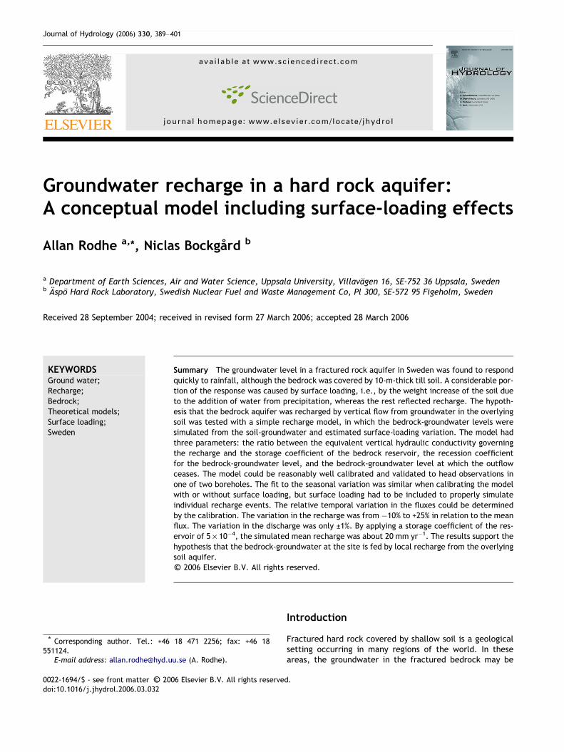
Three important simplifying assumptions were made forthe site under study: (1) the bedrock can be treated as acontinuous homogeneous medium in which the vertical flowis described by Darcy’s law, (2) Qin = 0, i.e., the site is onthe groundwater divide for the bedrock aquifer and (3)the bedrock aquifer behaves as a linear reservoir (Zoch,1934). The recharge is then approximated as

R ¼ Kvhs � hb

hs � h1ð2Þ

where Kv (m s�1) is the equivalent vertical hydraulic conduc-tivity between the groundwater table in the soil and the le-vel h1 (m) in the bedrock at which pressure is measured, andhs (m) and hb (m) are the groundwater levels in the soil andthe bedrock, respectively, expressed as height above anarbitrary reference level (Fig. 1). Note that hb, the ground-water level in the bedrock, is an effect of both surface load-ing and mass storage. The flow is generated by headgradients, regardless of the reasons for the head changes,and no corrections for surface loading should be made intheir calculations. The outflow from the linear reservoir isgiven by

Q out ¼ amðhb � h0Þ ð3Þ

where a (s�1) is a recession coefficient, m (�) is the storagecoefficient of the bedrock aquifer and h0 (m) is the ground-water level in the bedrock at which the flow ceases (Psealevel).

With the above assumptions Eq. (1) becomes

ðhs � hbÞðhs � h1Þ

¼ m

Kv

dh�bdtþ aðhb � h0Þ

� �ð4Þ

Here, hs and hb are measured variables, h1 is a known con-stant,m, Kv, a and h0 are parameters with physical interpre-tations. The assumptions underlying this equation could betested by investigating whether there exist values of a andh0 for which a plot of (hs � hb)/(hs � h1) versusdh�b=dtþ aðhb � h0Þ gives a straight line (the slope of whichrepresents m/Kv). The method is, however, crude sincethere is a considerable noise in dh�b related to random errorsin the groundwater level measurements and corrections for

Figure 1 Conceptual model for the water balance of acolumn of a semi-confined bedrock aquifer overlain by a soilaquifer. hs and hb are the groundwater levels in the soil and thebedrock respectively, h1 is the level of the dominating trans-missive zone in the bedrock or the level at which pressure ismeasured, and h0 is the groundwater level in the bedrock atwhich the flow ceases. R is recharge to the bedrock column andQout is outflow from the column.

loading pressure changes, giving a large scatter in the plot.An equivalent way to test the assumptions is to solve Eq. (4)numerically for h�b and investigate whether there existparameter values for which h�b modelled from hs can fit ob-served h�b.

Rearranging Eq. (4) and defining b = Kv/m gives

dh�bdt¼ b

hs � hb

hs � h1� aðhb � h0Þ ð5Þ

A successful simulation of h�b by this model, after tuning thethree parameters a, b, and h0, would support the assump-tions on which the model is based, i.e., that the bedrockaquifer is recharged by Darcian flow from the overlying soilaquifer and that it can be regarded as a linear reservoirwithout lateral inflow. Since the parameters have knownphysical meanings (a is the recession coefficient for bed-rock-groundwater level, b is Kv/m and h0 is the threshold le-vel for bedrock-groundwater drainage), it is possible todelineate reasonable ranges of their values when doingthe calibration.

If the assumptions have been supported, the relativevariations of the groundwater recharge over time can beestimated by Eq. (2) and those of the outflow by Eq. (3).Since only the quotient Kv/m can be obtained by the calibra-tion, and not Kv or m separately, it is not possible to calcu-late the absolute value of the flow, unless Kv or m has beenobtained by some other method such as pump test.

Site

The measurements were made at the Norunda NOPEX(Northern Hemisphere Climate-processes Land-surfaceExperiment) site (Halldin et al., 1999). The site (60�4 0N17�28 0E, alt. 50 m a.s.l.) is located in central Sweden about30 km north of Uppsala, as shown in Fig. 2. The nearestcoast, which is that of the Baltic Sea, is about 50 km tothe north-east. The site was selected for the present studysince it, according to the topography, could be expected tobe a recharge area for bedrock-groundwater. This was laterconfirmed by groundwater head measurements in the soiland bedrock-groundwater, showing a vertically downwardhead gradient. The availability to installations and infra-structure from the NOPEX project was a further factor inthe site selection. A detailed description of the site canbe found in Lundin et al. (1999). The area is situated onthe sub-Cambrian peneplain and is flat, with small-scalevariations in altitude of up to 10 m. The bedrock in the areais granite to granodiorite (unpublished data from the Geo-logical Survey of Sweden). The granite in the region is oftenrelatively permeable (SKB, 2000) and the hydraulic anisot-ropy of the bedrock is partly correlated to the prevailingrock stresses. Investigations in similar bedrock at anothersite in the region (SKB, 2005) have shown that the upper-most part of the bedrock often is more conductive thanthe overlying till, and strongly anisotropic with the highestconductivity value in the horizontal plane. Boreholesthrough the upper 100 m of the bedrock contain about threehigh transmissive fracture intercepts on average.

The soil at the site is a compact sandy till with a highcontent of stones and blocks. Lindahl (1996) estimated thehydraulic conductivity of the soil to be from 10�4 m s�1

Figure 2 Topographical map of the Norunda study area in Sweden (From the Topographical map�c Lantmateriverket Gavle 2004.Permission M2004/4515.) and a detail sketch of the soil and groundwater installations (modified from Bockgard, 2004).


(0–25 cm depth) to 10�6 m s�1 (95–120 cm depth). Thedeeper till layers may have considerably lower hydraulicconductivity, but there are no measurements from the site.The depth to the bedrock is about 10 m in two borings at themeasurement site. The till cover in the region is mostly be-tween 2 m and 10 m deep, and the largest known depth ofthe till in the 25 km · 25 km quaternary-map area is 13 m(SGU, 1989). There are no outcrops of bedrock within a ra-dius of approximately 1 km from the measurement site. Thesite is forested with mainly mature (about 75 year old)spruce and pine.

The mean air temperature in Uppsala was 5.6 �C for theperiod 1961–1990, and the mean annual precipitation15 km E of the site, not corrected for systematic measure-ment errors, was 587 mm (SHMI, 1991). The annual precipi-tation at the site for the same period, corrected formeasurement errors by the method of Eriksson (1988),was estimated to about 700 mm (Seibert, 1994). The meanrunoff in the region is about 250 mm yr�1 (SNA, 1995), givinga mean evapotranspiration of about 450 mm yr�1. Thegroundwater level in the soil aquifer at the site typicallyvaries between 0.1 and 1.5 m below ground surface duringthe year.

Measurements

The soil-groundwater level used for this study was moni-tored in a 3-m-deep groundwater tube with inner diameter53 mm located 30 m east of borehole C. The water level inthe tube was recorded using vented pressure transducers(Druck PDCR 1830 Series) connected to a Campbell CR10data logger (Campbell Scientific Inc.). The water level wasmeasured every 30 s, and 10-min averages were stored.The readings from the pressure transducer were calibratedregularly by manual soundings. The resolution in water levelwas 1 mm, and the uncertainty in the absolute water level,as estimated from the calibration, was about 3 mm.

Groundwater head in the bedrock was measured in two115-mm boreholes, borehole A (BhA) and borehole C (BhC)(Fig. 2). The boreholes A and C were drilled in March 2002

to total depths of 49 m and 40 m below ground surface,respectively. The soil depths at the boreholes were 12 mand 9.5 m, respectively. The boreholes were cased withsteel tubes extending about 3 m into the bedrock. The spacebetween the tube and the borehole wall was sealed usingcement grout in borehole C, while no sealing was made inborehole A.

The only fracture data available from the site are thoseobtained indirectly from a pump test and from boreholeflow loggings. Borehole flow logging showed that the onlymeasurable inflow to the boreholes, when pumping nearthe surface with a drawdown of the water table of a fewm, took place at one discrete level in each borehole. Inborehole A this transmissive zone was above the base ofthe casing, i.e., above 15 m depth. In borehole C the trans-missive zone was between 31.5 and 33.0 m. The concentra-tion of the transmissivity in the two boreholes to theselevels is probably not related to large-scale features, sincethe transmissive zones are close to the bedrock surface(borehole A) and have small vertical extensions (1 m inborehole C).

The recording of water levels started in April 2002. Bore-hole A was left open, while, in September 2002, borehole Cwas divided into four sections (0–15 m, 16–30 m, 31–33 m,34–40 m) using inflatable packers. The borehole sectionswere connected via 5-mm inner diameter polyamide tubingto 26-mm inner diameter polyethene standpipes, extendingfrom above the uppermost packer to the ground surface, inwhich the water level was monitored. The water levels inthe boreholes were monitored using the same type of sys-tem as in the soil-groundwater tube, with the differencethat, due to the lower resolution of the pressure transducerin borehole A, the resolution of the water level recordings inborehole A was 4 mm. Based on the results of the manualcalibrations, the uncertainty in absolute water level wasestimated to 5–12 mm.

The yield of the boreholes, with the water level near thebottom, was on the order of 5–10 L min�1. A pump test anda slug test were performed in borehole C. These tests wereroughly analysed with methods developed for homogeneous


media (pump tests by Cooper–Jacob method and slug testsby Bower–Rice and Cooper–Greene methods). Mean valuesof these tests gave a hydraulic conductivity of the bedrockof 3 · 10�7 m s�1 and a storage coefficient of 5 · 10�4, bothvalues referring to the layer penetrated by the well, i.e. forthe upper 30 m of the bedrock (unpublished data). Thecurve fitting was not improved when the pump test was ana-lysed by Hantush–Cooper method for an aquifer with leak-age, and consequently no estimate of the leakagecoefficient could be made.

The only extraction of bedrock or soil-groundwaterwithin a distance of at least 5 km from the site is for sin-gle or small groups of houses. With the nearest well lo-cated about 1.2 km from the study site the groundwatercan safely be regarded as natural, not affected by localhuman activities.

In addition to data from the above measurements, Bock-gard (2004) used records from the site of air pressure, airtemperature, soil-moisture content (see location Fig. 2),soil-groundwater levels (see location Fig. 2), snow storage,and winter precipitation from a nearby station, to estimatethe loading efficiency and the effect of surface loading onthe recorded groundwater levels in the bedrock. Consider-ing the similar topographic, soil, and vegetation conditionsaround the two boreholes, the used data on soil-moisturecontent and soil-groundwater levels can be assumed to berepresentative for both boreholes.

Effects of surface loading

As mentioned above, the model presented in this paper usesdata on the effects of surface loading as estimated by Bock-gard for this specific site. This section describes the meth-odology used for his estimates and comments upon theresults.

A changed load on the bedrock surface, for instance bychanges in soil moisture and rainfall interception or changein the atmospheric pressure, results in a changed verticalstress, rz (here expressed as metre water column), in thesoil or bedrock and its water. The stress change takes placeinstantaneously by grain to grain contact resulting in aninstantaneous pressure change, dP 0 (m), in the water. Thepressure change in the water due to mass flux of water(the diffusive pressure-change component dP) occurs withsome time delay. The instantaneous pressure change is gi-ven by

dP0

dt¼ c

drz

dtð6Þ

where c is the loading efficiency (�), expressing the part ofthe vertical stress change that is taken up by the water pres-sure (when there is no water flow induced by the stresschange). In the Norunda study, the total groundwater pres-sure was observed by measurements of the water level inboreholes or borehole sections open to the atmosphere. Achange in surface loading other than air pressure results ina proportional instantaneous water level change accordingto Eq. (6), where c is the constant of proportionality. Theconstant of proportionality for a change in air pressure pa,on the other hand, is Eb = (1 � c), the static-confined baro-metric efficiency. An increase in the atmospheric pressure

decreases the water level, whereas an increase in other sur-face loads increases the water level in the observation tube.

Bockgard (2004) estimated the loading efficiency c of thesoil and of the bedrock at the Norunda site from the re-sponse to atmospheric loading changes through the relationc = 1 � Eb. Since, under the prevailing semi-confined condi-tions, the barometric efficiency is dependent on time or fre-quency (the response for frequency going to infinity)(Rojstaczer, 1988), the analysis was done in the frequencydomain. The studied frequency range was 0.1–1 d�1, inwhich range the air pressure variation was the dominatingsurface-loading component. A three-layer model was usedto represent the site: (1) unsaturated soil 0–1 m, (2) satu-rated soil 1–10 m, and (3) bedrock >10 m depth.

The calculated loading efficiencies, being 0.87 for thesoil and 0.95 for the bedrock, were used to calculate theinstantaneous response in water level, h 0, from

h0 ¼ �ð1� cÞpa þ cr ð7Þ

and a residual well record h* (Rasmussen and Crawford,1997) from

h� ¼ h� h0 ð8Þ

where h is the observed water level record.The surface load, other than atmospheric pressure, was

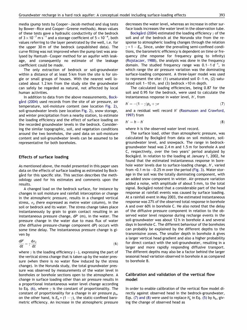
calculated by Bockgard from data on soil moisture, soil-groundwater level, and snowpack. The range in bedrock-groundwater head was 2.4 m and 1.5 m for borehole A andC, respectively, over the two years’ period analyzed byBockgard. In relation to the loading at January 1, 2002, hefound that the estimated instantaneous response in bore-hole water levels due to surface-loading change, h 0, variedfrom +0.1 m to �0.25 m over the period (Fig. 3). Water stor-age in the soil was the totally dominating component, withan added snow component in winter. Air-pressure variationadded a noise, with amplitude of about 5 mm, to the totalsignal. Bockgard noted that a considerable part of the headresponse at rainfall events was caused by surface loading.At a rainfall event in May 2003, the estimated instantaneousresponse was 27% of the observed total response in boreholeA and over 60% in borehole C. He also noted that the delayof the diffusive pressure component in relation to the ob-served water level response during recharge events in thesoil-groundwater was about 12 h in borehole A and severaldays in borehole C. The different behaviour of the boreholescan probably be explained by the different depths to thetransmissive zones. The smaller depth in borehole A givesa larger vertical head gradient and also a higher probabilityfor direct contact with the soil-groundwater, resulting in alarger and more rapidly responding diffusive transport.The different depths may also be a factor behind the largerseasonal head variation observed in borehole A as comparedto borehole B.

Calibration and validation of the vertical flowmodel

In order to enable calibration of the vertical flow model di-rectly against observed head in the bedrock-groundwater,Eqs. (7) and (8) were used to replace h�b in Eq. (5) by hb, giv-ing the change of observed head as

Figure 3 Calculated instantaneous response in borehole water level due to surface-loading changes. The dotted lines indicateestimated uncertainty (from Bockgard, 2004).


dhb

dt¼ b

hs � hb

hs � h1� aðhb � h0Þ þ c

drz

dt� ð1� cÞ dpa

dtð9Þ

where the sum of the last two terms represents the headchange due to surface loading. The time series of theseterms as calculated by Bockgard (2004) (see Fig. 3) was usedfor the modelling of hb. Eq. (9) was solved numerically for hbwith a time step of 30 min, which was the resolution of thesurface-load data.

The model was calibrated separately against groundwa-ter heads in borehole A and C, using soil- and bedrock-groundwater data from April 4, 2002 to December 14,2003. Soil-groundwater level in the observation tube 30 meast of borehole C (see Fig. 2) was taken as hs. The ground-water head in borehole A was measured in the open bore-hole and assumed to represent the most transmissive partof the borehole, at 14–15 m below the ground surface. Inborehole C, the head was measured as the water level inthe open borehole until September 2002, when the packerswere installed. For the remaining period, the head observedin the section representing the most transmissive part of theborehole, 31–33 m below the ground surface, was used. Thelevel h1 in Eq. (9) was put to 15 m below the ground surfacefor borehole A and to 32 m below the surface for boreholeC.

Short gaps in the data series on bedrock-groundwaterwere filled and spikes removed using linear interpolation.Long gaps (>one week), due to instrument failure or manip-ulated water levels caused by pumping tests, were left un-filled. There are prominent within-day fluctuations in thebedrock-groundwater heads due to Earth tides. These fluc-tuations, having amplitudes up to 10 mm, were left unfil-tered in the analysis. Since the tidal effect is not includedin the flow model, the tidal fluctuations reduce the good-ness of fit between simulated and observed groundwaterhead. This effect is small, however, since the fluctuationsare small compared to commonly occurring differences be-tween the simulated and observed heads.

Data from the period December 14, 2003 to July 29, 2004were used for validation of the model. Since the data on soilwater and snow storage were not processed for this period,the effect of surface load could not be calculated. Valida-tion was therefore done for a model without surface load-

ing. The surface loading terms of Eq. (9) were then put tozero during both calibration and validation.

The calibration was performed using Monte Carlo tech-niques. Possible ranges of each parameter value were de-fined based on their physical interpretations and theconditions at the site. Fifty thousand parameter sets weregenerated using random numbers from a uniform distribu-tion within the range given for each parameter. The Nashand Sutcliffe (1970) criteria

Reff ¼ 1�Pðhb;obs � hb;simÞ2Pðhb;obs � hb;obsÞ2

ð10Þ

here called efficiency, where subscript obs stands for ob-served and sim for simulated, was used as objective func-tion for the goodness of fit. The value of Reff is 61, withReff = 1 denoting a perfect fit. The parameter set givingthe highest value of Reff was searched for in the calibration.

The parameter h0 represents the head at which thedrainage of the bedrock aquifer goes to zero. The upper lim-it is the lowest observed head and the lower limit was ex-pected to be sea level. The local height system used inthis paper was defined such that the ground surface at bore-hole C, lying about 50 m a.s.l., is 10.0 m. The sea level isthus about �40 m in the local height system.

The lower limit for the recession coefficient for bedrock-groundwater head, parameter a, was estimated from theobserved head record. Since a represents the recession fora groundwater reservoir without inflow, but the rechargeis P0, a was expected to be larger than or equal to therecession coefficient obtained from the observed rate ofhead decline. With h0 = �40 m, the observed recession coef-ficients in the boreholes were about 3 · 10�9 s�1.

The parameter b = Kv/m was delimited by reasonableranges of the equivalent vertical hydraulic conductivity,Kv, between the groundwater level in the soil and the obser-vation level in the bedrock and of the storage coefficient,m. Based on the indicative values of hydraulic conductivityand storage coefficient of the bedrock available for the site,and general information from comparable fractured crystal-line rock, a wide range of values of b was considered possi-ble, from 10�8 to 10�3 m s�1.


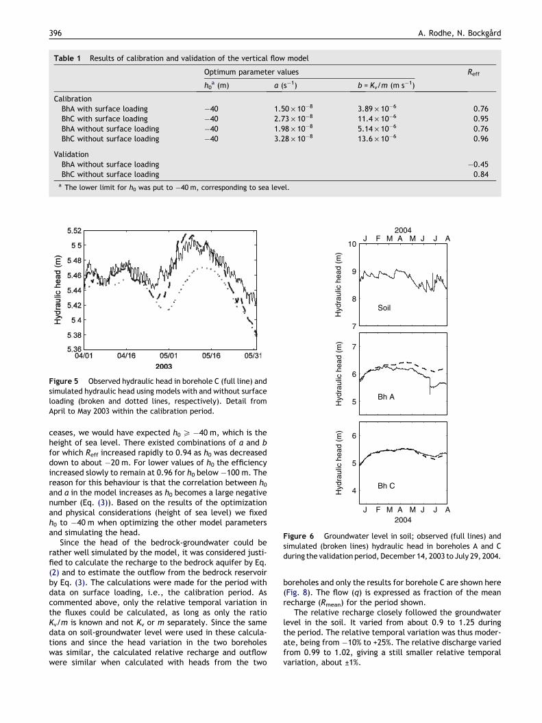
Results

It was possible to find parameter sets for which the ob-served head in the boreholes could be reasonably well sim-ulated from the observed soil-groundwater level at thegroundwater tube 30 m east of borehole C for the calibra-tion period, April 4, 2002 to December 14, 2003 (Fig. 4,Table 1). The model could simulate recharge events fairlywell, but it was less successful during recession periods.The simulated seasonal decline was too rapid at thebeginning of the study period, in spring 2002, and too slowduring the autumn periods. In borehole A there were consid-erable deviations during recession in early fall 2003, but themodel recovered after a sudden rise in the borehole head le-vel in October. This rise, which was not related to a rise inthe groundwater level in the soil, occurred immediatelyafter a few hours of pumping in the borehole for watersampling.

When calibrating the model without taking surface load-ing into account, i.e., putting the two last terms of Eq. (9)to zero, the visual impression of the fit was similar as forsimulations with surface loading, and the efficiency wasvery similar (Table 1). Recharge events could, however,

A M J J A S O N D J F

7

8

9

10

)m(

daehciluardy

H

5

6

7)m(

daehciluardy

H

A M J J A S O N D J F

4

5

6)m(

daehciluardy

H

2002

Figure 4 Groundwater level in soil; observed (full lines) and simulamodel with surface loading during the calibration period, April 4, 2

not be well simulated when surface loading was disre-garded, as exemplified by the event in early May 2003shown in enlarged scale in Fig. 5. (Note the Earth-tide fluctu-ations in the observed hydraulic headwhich are not accountedfor in the model.) Without surface loading, the simulatedhead response was delayed as compared to observations andsimulations with surface loading, with the peak of the mainevent occurring about 3 days after the observed peak.

As mentioned above, the model without surface loadingwas used for the validation (with the corresponding param-eter sets), since there were no surface-loading data avail-able for the validation period. The fit was fairly good forborehole C, with a somewhat lower efficiency than for thecalibration period. For borehole A, however, the model fitwas poor. (Fig. 6, Table 1).

The optimum value of the parameter b was quite welldetermined from the calibrations, as shown by the sharppeak in the plot of Reff versus the parameter value, exempli-fied in Fig. 7 (similar shapes were obtained for the other cal-ibrations of the parameters). For a and h0, on the otherhand, the optimum values were less distinct due to the cor-relation between these parameters. With h0 representingthe head at which the outflow from the bedrock aquifer

M A M J J A S O N D J

Soil

Bh A

M A M J J A S O N D J

Bh C

2003

ted (broken lines) hydraulic head in boreholes A and C using the002 to December 14, 2003.

J F M A M J J A

7

8

9

10

)m(

daehciluardy

H

2004

Soil

5

6

7)

m(daeh

ciluardyH

Bh A

J F M A M J J A

4

5

6

)m(

daehciluardy

H

Bh C

2004

Figure 6 Groundwater level in soil; observed (full lines) andsimulated (broken lines) hydraulic head in boreholes A and Cduring the validation period, December 14, 2003 to July 29, 2004.

Table 1 Results of calibration and validation of the vertical flow model

Optimum parameter values Reff

h0a (m) a (s�1) b = Kv/m (m s�1)

CalibrationBhA with surface loading �40 1.50 · 10�8 3.89 · 10�6 0.76BhC with surface loading �40 2.73 · 10�8 11.4 · 10�6 0.95BhA without surface loading �40 1.98 · 10�8 5.14 · 10�6 0.76BhC without surface loading �40 3.28 · 10�8 13.6 · 10�6 0.96

ValidationBhA without surface loading �0.45BhC without surface loading 0.84

a The lower limit for h0 was put to �40 m, corresponding to sea level.

Figure 5 Observed hydraulic head in borehole C (full line) andsimulated hydraulic head using models with and without surfaceloading (broken and dotted lines, respectively). Detail fromApril to May 2003 within the calibration period.


ceases, we would have expected h0 P �40 m, which is theheight of sea level. There existed combinations of a and bfor which Reff increased rapidly to 0.94 as h0 was decreaseddown to about �20 m. For lower values of h0 the efficiencyincreased slowly to remain at 0.96 for h0 below �100 m. Thereason for this behaviour is that the correlation between h0and a in the model increases as h0 becomes a large negativenumber (Eq. (3)). Based on the results of the optimizationand physical considerations (height of sea level) we fixedh0 to �40 m when optimizing the other model parametersand simulating the head.

Since the head of the bedrock-groundwater could berather well simulated by the model, it was considered justi-fied to calculate the recharge to the bedrock aquifer by Eq.(2) and to estimate the outflow from the bedrock reservoirby Eq. (3). The calculations were made for the period withdata on surface loading, i.e., the calibration period. Ascommented above, only the relative temporal variation inthe fluxes could be calculated, as long as only the ratioKv/m is known and not Kv or m separately. Since the samedata on soil-groundwater level were used in these calcula-tions and since the head variation in the two boreholeswas similar, the calculated relative recharge and outflowwere similar when calculated with heads from the two

boreholes and only the results for borehole C are shown here(Fig. 8). The flow (q) is expressed as fraction of the meanrecharge (Rmean) for the period shown.

The relative recharge closely followed the groundwaterlevel in the soil. It varied from about 0.9 to 1.25 duringthe period. The relative temporal variation was thus moder-ate, being from �10% to +25%. The relative discharge variedfrom 0.99 to 1.02, giving a still smaller relative temporalvariation, about ±1%.

Figure 7 Model efficiency Reff against the values of the model parameters. Each dot represents a combination of a, b, and h0 givinga specific value of Reff.

A M J J A S O N D J F M A M J J A S O N D J0

0.2

0.4

0.6

0.8

1

1.2

20032002

R/qnae

m

Figure 8 Simulated groundwater recharge to the bedrock (full line) and outflow from the bedrock reservoir (broken line) forborehole C, modelling with surface loading for the calibration period. The flow, q, is normalized by the mean recharge, Rmean.


Discussion

The finding that the observed head of the bedrock-groundwater could be simulated by the model supportsthe assumptions underlying the model. It is thus notunrealistic to assume that the bedrock-groundwater atthe site is fed by local recharge from the overlying soilaquifer, driven in a Darcyan way by the head gradientbetween soil-groundwater and bedrock-groundwater, andthat the outflow from the reservoir is proportional tothe groundwater head above some reference level. Theapproximation of the bedrock as a continuous porousmedium with a vertical hydraulic conductivity is not phys-ically realistic in this scale, but with laminar flow in thefractures there is some justification for defining an equiv-alent vertical hydraulic conductivity for the boreholeresponse.

In borehole A, the head seems to have been unstable.Two events with anomalous sudden head changes were ob-served in this borehole, on October 2, 2003 (Fig. 4) and on

June 16, 2004 (Fig. 6). Both events occurred directly aftershort pumpings for water sampling in the borehole. In thefirst event, a temporary packer was installed 16 m belowthe ground surface and water was pumped for samplingabove this level. After 4 h the pumping was stopped andthe packer was removed, leaving the borehole open as itwas before the sampling. The water level rose quickly, pass-ing the initial level after a few hours, and after 3 days itreached a constant value 0.6 m above the initial level.During the period with anomalous rise, and also the weekbefore, there were no large rainfall events and the soil-groundwater level receded continuously. After the event,the bedrock-groundwater head receded continuously forabout one month. The rate of recession was somewhatslower than before the event, probably due to rainfallevents causing moderate raisings of the soil-groundwater le-vel. The second event was initiated by a 40 min lowering ofthe water table by at most 0.7 m in response to pumping forwater collection. After the pumping, the groundwater leveldid not recover to the initial level, but rose to a level 0.3 m


below the initial one, after which the recession precedingthe event continued.

In borehole C, there were no obvious anomalies in thegroundwater head and the model fitting and validation forthis borehole were quite good. Regarding the anomalouschanges in the head in borehole A, during the calibrationperiod, as well as during the validation period, it is notunexpected that the model fitting and validation were lesssuccessful for this borehole. The only reasons we can findfor this anomalous behaviour are related to the connectionbetween the borehole and the bedrock-groundwater. A ten-tative explanation is that some water supplying fracture wasblocked during the recession period of June to October 2003and that this blocking was released when the water levelwas lowered by the pumping on October 2. After that datethe water level might have returned to the ‘‘normal’’ level.With a similar speculation, the decline in June 2004 couldhave been caused by changes in the fracture openings trig-gered by the pumping. Since any selection of periods with‘‘normal’’ behaviour would have been subjective, we choseto use the whole original period for calibration of boreholeA, accepting bad fitting for this borehole and focusing thediscussion and conclusion on the results from borehole C.

The efficiency Reff, used as the objective function for thegoodness of fit for finding optimal parameter sets, is usefulhere for capturing the seasonal variations. It is, however,less useful for comparing the two model approaches: withand without surface loading. The fitting was very similaron a seasonal basis for the two approaches (the differencebetween the two simulations is hardly seen if the headsare plotted in the scale of Fig. 4) and the Reff values werevery similar, 0.95 with and 0.96 without surface loading (Ta-ble 1). When using Reff as objective function, the optimiza-tion emphasizes the large seasonal variations, whereas thecomparatively small dynamics of recharge events is littleaccounted for. The comparatively good fit of rechargeevents when including surface loading in the model is there-fore not seen in the values of Reff. The efficiency may fur-ther give little information when different time periodsare compared. The temporal variability of the variable un-der study must be large and frequent enough and the timeperiod long enough for making Reff independent of thechoice of time period. These criteria were not fulfilled here,neither for the calibration nor the validation period.

Although surface loading was necessary to model thehead variation during events, the fit during some eventswas moderate also when surface loading was included. Itis probable that one could find criteria which could improvethis fitting, but no such attempts were made here. Whenjudging the fitting one should also consider the uncertaintyin the estimated effect of surface load on the head. Impor-tant parts of this uncertainty are uncertainties in the esti-mated loading efficiency, c, and the areal mean value ofsoil-moisture content. The uncertainty in the estimated ef-fect of the atmospheric loading differs from that of the soil-moisture loading. The air pressure is measured with highaccuracy and it is perfectly representative for the site.The barometric efficiency, Eb, as determined by Bockgard(2004), was 0.05 ± 0.03. The relative uncertainty in Eb isthus ±60%, which is directly propagated to the calculated ef-fect of the atmospheric loading (Eq. (9)). Since the value ofthe loading efficiency, 0.95, was determined as 1 � Eb, the

absolute uncertainty is the same as for Eb, giving a relativeuncertainty in c of ±3%. The absolute values of the effect ofthe atmospheric loading are thus uncertain, whereas theshape of the temporal variations is well determined. Theloading efficiency, on the other hand, is comparativelyaccurate, but uncertainty in the calculated soil-moisturecontent related to measurements and representativity con-tributes to uncertainty in the absolute value of the effect ofthe soil-moisture loading.

In Fig. 5, the observed head and the head modelled withsurface loading for an event was compared with the headmodelled without taking surface loading into account. Theevent is further analyzed in Fig. 9, showing the head andits components as modelled with surface loading duringthe same episode. The dominant role of the soil-moistureloading (including soil-groundwater) in the head responsecan be seen in the figure. The very first head rise was causedby a decline in the atmospheric pressure by about 35 hPacontributing with 18 mm, marked by (a), to the head rise(partly counteracted by the declining diffusive component).The following rapid rise in the simulated head was due to in-creased soil-water loading caused by rainfall. A measuredrainfall of 67 mm during the period April 26 to May 7, 2003gave an observed increase in soil-water content (includingsoil-groundwater storage) of 65 mm. (The small differencebetween rainfall and increase in soil-water content, 2 mm,is not realistic since there certainly was some evapotranspi-ration during the period. The inconsistency can be explainedby measurement and representativity errors for rainfall and,particularly, soil-water content.) With the estimated load-ing efficiency of 0.95, the measured soil-water loading gen-erated a head rise of 62 mm (b). The simulated diffusivecomponent, finally, contributed to a head rise of 40 mm(c), peaking about 5 days after the simulated total head.

A more direct way to estimate the diffusive component isto subtract the estimated effects of surface loading fromthe observed head, i.e., to calculate the so-called residualwell record (Eq. (8)), shown by the thick line in Fig. 9. Ina perfect model, the diffusive component would equal theresidual well record (corrected for tidal fluctuations). Thefit is, however, comparatively poor here, with the residualwell record being delayed by about 5 days compared tothe diffusive component, showing limitations of the model.

The parameter a, the recession coefficient, depends onthe value of h0 due to the correlation between these param-eters. The optimal value of a with h0 = �40 m was2.73 · 10�8 s�1 for borehole C. As expected, this value is lar-ger than the corresponding coefficient describing the ob-served decline of the head in late summer (withh0 = �40 m). This is so since the observed decline of thehead does not represent a pure reservoir emptying (de-scribed by a) but represents the decline of a reservoir withinflow. This inflow, the recharge from the overlying soilaquifer, took place continuously since the bedrock-ground-water head was always lower than that of the soil (Figs. 4and 6).

As commented above, the relative variations in the esti-mated recharge to the bedrock-groundwater were quitesmall (Fig. 8). This is a direct consequence of the small rel-ative variations in the vertical head gradient, i.e., essen-tially in the relative variations in the difference betweenthe heads in the soil and bedrock-groundwater. The relative

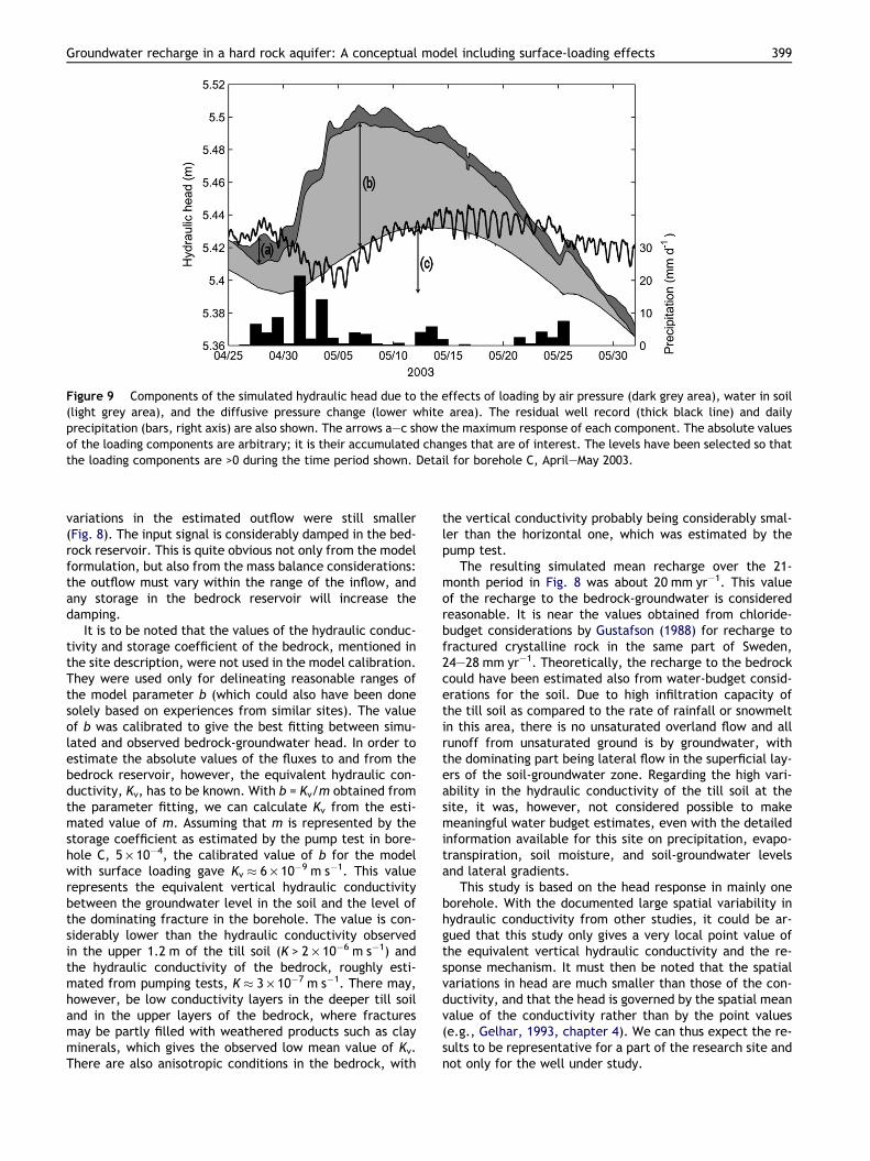
Figure 9 Components of the simulated hydraulic head due to the effects of loading by air pressure (dark grey area), water in soil(light grey area), and the diffusive pressure change (lower white area). The residual well record (thick black line) and dailyprecipitation (bars, right axis) are also shown. The arrows a–c show the maximum response of each component. The absolute valuesof the loading components are arbitrary; it is their accumulated changes that are of interest. The levels have been selected so thatthe loading components are >0 during the time period shown. Detail for borehole C, April–May 2003.


variations in the estimated outflow were still smaller(Fig. 8). The input signal is considerably damped in the bed-rock reservoir. This is quite obvious not only from the modelformulation, but also from the mass balance considerations:the outflow must vary within the range of the inflow, andany storage in the bedrock reservoir will increase thedamping.

It is to be noted that the values of the hydraulic conduc-tivity and storage coefficient of the bedrock, mentioned inthe site description, were not used in the model calibration.They were used only for delineating reasonable ranges ofthe model parameter b (which could also have been donesolely based on experiences from similar sites). The valueof b was calibrated to give the best fitting between simu-lated and observed bedrock-groundwater head. In order toestimate the absolute values of the fluxes to and from thebedrock reservoir, however, the equivalent hydraulic con-ductivity, Kv, has to be known. With b = Kv/m obtained fromthe parameter fitting, we can calculate Kv from the esti-mated value of m. Assuming that m is represented by thestorage coefficient as estimated by the pump test in bore-hole C, 5 · 10�4, the calibrated value of b for the modelwith surface loading gave Kv � 6 · 10�9 m s�1. This valuerepresents the equivalent vertical hydraulic conductivitybetween the groundwater level in the soil and the level ofthe dominating fracture in the borehole. The value is con-siderably lower than the hydraulic conductivity observedin the upper 1.2 m of the till soil (K > 2 · 10�6 m s�1) andthe hydraulic conductivity of the bedrock, roughly esti-mated from pumping tests, K � 3 · 10�7 m s�1. There may,however, be low conductivity layers in the deeper till soiland in the upper layers of the bedrock, where fracturesmay be partly filled with weathered products such as clayminerals, which gives the observed low mean value of Kv.There are also anisotropic conditions in the bedrock, with

the vertical conductivity probably being considerably smal-ler than the horizontal one, which was estimated by thepump test.

The resulting simulated mean recharge over the 21-month period in Fig. 8 was about 20 mm yr�1. This valueof the recharge to the bedrock-groundwater is consideredreasonable. It is near the values obtained from chloride-budget considerations by Gustafson (1988) for recharge tofractured crystalline rock in the same part of Sweden,24–28 mm yr�1. Theoretically, the recharge to the bedrockcould have been estimated also from water-budget consid-erations for the soil. Due to high infiltration capacity ofthe till soil as compared to the rate of rainfall or snowmeltin this area, there is no unsaturated overland flow and allrunoff from unsaturated ground is by groundwater, withthe dominating part being lateral flow in the superficial lay-ers of the soil-groundwater zone. Regarding the high vari-ability in the hydraulic conductivity of the till soil at thesite, it was, however, not considered possible to makemeaningful water budget estimates, even with the detailedinformation available for this site on precipitation, evapo-transpiration, soil moisture, and soil-groundwater levelsand lateral gradients.

This study is based on the head response in mainly oneborehole. With the documented large spatial variability inhydraulic conductivity from other studies, it could be ar-gued that this study only gives a very local point value ofthe equivalent vertical hydraulic conductivity and the re-sponse mechanism. It must then be noted that the spatialvariations in head are much smaller than those of the con-ductivity, and that the head is governed by the spatial meanvalue of the conductivity rather than by the point values(e.g., Gelhar, 1993, chapter 4). We can thus expect the re-sults to be representative for a part of the research site andnot only for the well under study.


With a long term mean runoff in this region of about250 mm yr�1, a continuous leakage from the soil-groundwa-ter on the order of 20 mm yr�1 in recharge areas for bed-rock-groundwater would have no noticeable effect on theflow in the soil and the streams. The recharged bedrock-groundwater will eventually be discharged in low-lyingareas and contribute to streamflow (and evapotranspira-tion) further down in the catchment or it may be dis-charged directly to the sea, thus being withdrawn fromsoil moisture and stream runoff. For understanding howbedrock-groundwater recharge and flow affects the waterbudget on a catchment or regional scale, extensive infor-mation on groundwater levels and hydraulic properties ofthe ground are needed and good groundwater modellinghas to be performed.

The main reason for using the model presented in this pa-per was to test the whether the observed head variations inthe bedrock aquifer could be explained by vertical rechargeand surface-loading effects. Although the model is very sim-ple it was useful for that purpose. It could probably be usedto analyze the head response in other recharge areas forbedrock-groundwater, where the bedrock aquifer is overlainby a soil cover with groundwater. Equally detailed soil-mois-ture data are seldom available, but since the water contentof the unsaturated zone to a large degree is controlled bythe level of a shallow groundwater table (e.g., Beldringet al., 1999), it might be possible to develop and use empir-ical relationships between soil-groundwater level and soil-moisture load. Furthermore, since the seasonal variationin head could be well simulated also without accountingfor the surface load, the model could be used without dataon the soil-moisture load if the head response during eventsis not looked for.

Conclusions

The observed head of the bedrock-groundwater could befairly well simulated from the groundwater level in theoverlying soil by a model based on vertical flow drivenby the head gradient between the soil-groundwater andthe bedrock-groundwater. The results support thehypothesis that the bedrock-groundwater at the site isfed by local recharge from the overlying soil aquiferand that the outflow from the bedrock-groundwater res-ervoir is proportional to the groundwater head abovesome reference level. It should be noted, however, thatthe model is conceptual and based on the simplifyingassumption that the fractured bedrock, from a rechargepoint of view, can be treated as a continuous porousmedium.

The seasonal head variation could be simulated equallywell with or without the effect of surface loading. Simula-tion of the head dynamics during recharge events was, how-ever, considerably improved when taking surface loadinginto account. The effect of increased surface loading, dueto the increased water storage in the soil, was the dominat-ing component of the head response in the bedrock-ground-water during rainfall events.

The recharge to the bedrock aquifer took place con-tinuously, with only small relative variations over theyear.

Acknowledgements

This study was funded by the Geological Survey of Sweden(SGU) under contract 03-1139/2000. The authors thank Geo-sigma AB for advice and providing field equipment. We arealso grateful to S.-Y. Hamm and an anonymous reviewerfor constructive and helpful comments on the manuscript.

References

Alley, W.M., Healy, R.W., LaBaugh, J.W., Reilly, T.E., 2002. Flowand storage in groundwater systems. Science 296, 1985–1990.

Barker, J.A., 1988. A generalized radial flow model for hydraulictests in fractured rock. Water Resour. Res. 24 (10), 1796–1804.

Beldring, S., Gottschalk, L., Seibert, J., Tallaksen, L.M., 1999.Distribution of soil moisture and groundwater levels at patch andcatchment scales. Agric. Forest Meteor. 98–99, 305–324.

Bockgard, N., 2004. Groundwater Recharge in Crystalline Bedrock:Processes, Estimation, and Modelling. Ph.D. Thesis, Comprehen-sive Summaries of Uppsala Dissertations from the Faculty ofScience and Technology 1019, Uppsala University, Uppsala, 48pp.

Eriksson, B., 1988. Data rorande Sveriges nederbordsklimat. Nor-malvarden for perioden 1951–80. [Data on the PrecipitationClimate of Sweden. Normal Values for the Period 1951–80.].Swedish Meteorological and Hydrological Institute, Climatedivision Report 1983:28 (in Swedish).

Gburek, W.J., Folmar, G.J., 1999. A ground water recharge fieldstudy: site characterization and initial results. Hydrol. Process.13, 2813–2831.

Gelhar, L.W., 1993. Stochastic Subsurface Hydrology. Prentice-Hall, Englewood Cliffs, NJ, 390 pp.

Gustafson, G., 1988. Groundwater in crystalline rocks – some ideas.In: Englund et al. (Eds.), Studies on Groundwater Recharge inFinland, Norway and Sweden. Proceedings of a Workshop,Mariehamn, Aland, Finland, 25–26 September 1986, Helsinki,pp. 91–97.

Halldin, S., Gryning, S.E., Gottschalk, L., Jochum, A., Lundin, L.-C., Van de Griend, A.A., 1999. Energy, water and carbonexchange in a boreal forest – NOPEX experiences. Agric. ForestMeteorol. 98–99, 5–29.

Hamm, S.-Y., Bidaux, P., 1996. Dual-porosity fractal models fortransient flow analysis in fissured rocks. Water Resour. Res. 32(9), 2733–2745.

Hantush, M.S., 1956. Analysis of data from pumping tests in leakyaquifers. Trans. Am. Geophys. Union 37 (6).

Harte, P.T., Winter, T.C., 1995. Simulations of flow in crystallinerock and recharge from overlying glacial deposits in a hypothet-ical New England setting. Ground Water 33 (6), 953–964.

Johansson, P.-O., 1987. Methods for estimation of natural ground-water recharge directly from precipitation; comparative studiesin sandy till. In: Simmers, I., (Ed.), Estimation of NaturalGroundwater Recharge. NATO ASI Series. Series C: Mathematicaland Physical Sciences 222, pp. 239–270.

Lee, J.-Y., Lee, K.-K., 2000. Use of time series data for identifi-cation of recharge mechanism in a fractured bedrock aquifersystem. J. Hydrol. 229, 190–201.

Lerner, D.N., Issar, A.S., Simmers, I., 1990. Groundwater recharge.A guide to understanding and estimating natural recharge.International Contributions to Hydrogeology, vol. 8, VerlagHeise, Hannover.

Lindahl, A., 1996. Modellering av avdunstning utgaende franmarkfuktighetsmatningar i moranmark [Modeling of evaporationbased on soil moisture measurements in a till soil]. M.Sc. Thesis,Department of Earth Sciences, Uppsala University, Sweden (inSwedish).


Lundin, L.-C., Halldin, S., Lindroth, A., Cienciala, E., Grelle, A.,Hjelm, P., Kellner, E., Lundberg, A., Molder, M., Moren, A.-S.,Nord, T., Seibert, J., Stahli, M., 1999. Continuous long-termmeasurements of soil-plant-atmosphere variables at a forestsite. Agric. Forest Meteor. 98–99, 53–73.

Nash, J.E., Sutcliffe, J.V., 1970. River flow forecasting throughconceptual models, Part I – A discussion of principles. J. Hydrol.10, 282–290.

Rasmussen, T.C., Crawford, L.A., 1997. Identifying and removingbarometric pressure effects in confined and unconfined aquifers.Ground Water 35 (3), 502–511.

Rojstaczer, S., 1988. Determination of fluid flow properties fromthe response of water levels in wells to atmospheric loading.Water Resour. Res. 24 (11), 1927–1938.

Seibert, P., 1994. Hydrological Characteristics of the NOPEXResearch Area. M.Sc. Thesis, Department of Earth Sciences,Uppsala University, Sweden.

SGU, 1989. Quaternary Map Soderfors SO. Geological Survey ofSweden, SGU Ser. Ae nr 104, Uppsala, Sweden.

SHMI, 1991. Temperaturen och nederborden i Sverige 1961–90Referensnormaler [Temperature and Precipitation in Sweden1961–90. Reference normals]. SMHI Meteorologi, 81 (inSwedish).

SKB, 2000. Forstudie Osthammar – Slutrapport [Pre-investiga-tion Osthammar – Final Report]. Swedish Nuclear Fuel andWaste Management Co (SKB), Stockholm, Sweden (inSwedish).

SKB, 2005. Preliminary Site Description. Forsmark Area – Version1.2. Updated 2005-11-09. SKB R-05-18. Swedish Nuclear Fuel andWaste Management Co (SKB), Stockholm, Sweden.

SNA, 1995. Klimat, sjoar och vattendrag [Climate, Lakes and WaterCourses]. Sveriges Nationalatlas. Bokforlaget Bra Bocker, Hoga-nas, Sweden, ISBN 91-87760-31-2 (in Swedish).

Tiedeman, C.R., Goode, D.J., Hsieh, P.A., 1998. Characterizing aground water basin in a New England mountain and valleyterrain. Ground Water 36 (4), 611–620.

Zoch, R.T., 1934. On the relation between rainfall and stream flow.Monthly Weather Rev. 62, 315–322.

groundwater recharge in a hard rock aquifer: a conceptual model including surface-loading effects

Documents