groundwater investigation by using resistivity survey in

Journal of Resources Development and Management - An Open Access International Journal

Vol.2 2013

9

Groundwater Investigation by Using Resistivity Survey in

Peshawar, Pakistan

Gul Daraz Khan1, Waheedullah

1, Asher Samuel Bhatti

2

1 Department of Water Management, Faculty of Crop Production Sciences, The University of Agriculture,

Peshawar-Pakistan

2 Department of Geology, Bacha Khan University Charsadda, Pakistan.

Corresponding E-mail: [email protected]

Abstract

Resistivity survey was conducted in Peshawar to investigate groundwater using Terrameter SAS 4000. Six sites

were selected for the studies through feasibility survey to identify feasible points for conducting survey. Data

collected was analyzed using 1X1D software which uses principal of conventional theory of curve matching.

Resistivity values were compared with standard table of resistivity values of geological formations through

which depths to water table was estimated, which were compared to the existing surrounding wells. These local

results showed that shallow depths estimated for groundwater table were at Pakistan Forest Institute as saturated

sand and gravel, for an average depth to water table of 23 m with respect to ground surface. In University

Campus/Professor Colony, Biotechnology, Hayatabad Township site 1, and Site 2 the local groundwater level

mostly in sand and gravel materials were at depths of 41 m, 37 m, 92 m and 82 m for different resistivity values.

Study concludes that Instead of natural surface flow and seepage, there should be storage in the permeable zone

or open dug wells within the planned storages for artificial recharge. Furthermore use of geophysical tools for

groundwater investigation provides easy and quick approach as compared to conventional methods of

groundwater investigations.

Keywords: Groundwater. Resistivity survey. Terrameter SAS 4000. 1X1D software. Geophysical tools.

Georefrencing.

INTRODUCTION

Groundwater is that water which occurs beneath the surface of earth in saturated zones where the

hydrostatic pressure is equal to or more than atmospheric pressure. It is believed that groundwater exists in large

lakes or pools under the surface of earth. The truth is that it exists in pore spaces and fractures in rocks (Tyson,

1993). Pakistan is basically an agriculture country where the contribution of agriculture commodities to the

country Gross Domestic Product (GDP) is about 21.8% and is the source of earning for 44.7% of the manpower

employed (PES, 2009). The availability of water per head in Pakistan has also been reduced from 5200m3 in

1950 to 1000m3 in 2001 (WRL, 2001). More-over most parts of the country lies in arid to semi arid climate

where there is a lot of variation in the rainfall which ranges from 150mm in southern area to 750mm in northern

areas. Water quality is more probably a serious problem in case when the pumpage rate exceeds the natural

recharge in droughts seasons. The water table goes down to a depth to 5-7 meter in some parts of the country.

(Bakhsh and Awan, 2002). The reason for such changes in water quality is the over pumping of fresh water

which replace that water from saline and deteriorated zones (Ahmed and Kutcher, 1992). Ground water quality

in some areas is worse than canal water containing salts. Hence, in such areas ground water may be a serious

threat to agricultural lands and utilizing ground water would result in adding more salts to soils.(Bakhsh and

Awan, 2002).

The resistivity survey technique is used to solve many problems related to groundwater assessment,

investigation, exploration and salinity. Some uses of this method in groundwater are; determination of the

thickness, boundary and depth of different layers of an aquifer (Zohdy, 1969; Young et al., 1998; Soupios, 2007),

determination of boundary line between saline water and fresh water (El- Waheidi et al., 1992; Choudh`ury et al.,

2001) and contamination of groundwater (Kelly, 1976; Kaya, 2001). Contamination usually reduces the

electrical resistivity of pure water due to increase of the ion concentrations (Lashkaripour, 2003; Oseji et al.,

2006; Park et al., 2007). Relationship between aquifer characteristics like transmissivity and conductivity,

lithology and other parameters in combination with geo electrical parameters are studied and reviewed by many

researchers and authors for exploration and determination of ground water quality and suitability for different

aspects (Kelly, 1976; Niwas and Singhal, 1981; Onuoha and Mbazi, 1988). Geophysical studies reveal the

importance of resistivity method in ground water assessment in alluvial soils. Resistivity survey also shows great

success in settling wells in areas underlain by hard rock terrains (Flathe, 1954; Meidav, 1960; Van Dam and

Meulenkamp, 1967; Vincenz, 1968; Zohdy 1969; Serres, 1969;). Electrical resistivity method is widely used to

solve variety of ground water problems such as assessment of strata, depth, thickness and boundaries of aquifer,

estimation of boundaries between fresh and saline water zones (El-Waheidi et al., 1992), determination of high

yield potential zones in an aquifer (Oseji, 2005), and exploration of ground water quality (Arshad et al., 2007).

The proposed study was designed to investigate the groundwater in different regions selected


Vol.2 2013

10

purposively in Peshawar on the basis of accecesibility and field trnasportation. Where the study was conducted

with the following objectives.

• Assessment of groundwater levels in selected areas by using resistivity survey.

• Identification of groundwater bearing strata in study area.

MATERIALS AND METHODS

Site Description

The sites for the propsed study were choosed at various locations in district Peshawar on the basis of

accesibility and field logistics. The given topo map in figure 1 shows the different positions of the profiles

surveyed along with thier names, where further detail data was acquired. The area has been divided into three

main sites. The site No.1 mainly includes the Pakistan Forest Institute (PFI 1 and PFI 2) locations were selected

for executing field survey. The second site was selected in close vicinity of the University region where two sites

were selected for survey. The third location of Hayatabad township which includes six locations where extended

detailed field field survey was launched. A total of six locations have been selected in the whole region including

Pakistan Forest Institute (2), Biotechnology and New Professor Colony (2) and different phases of hayatabad (2).

The elevation of the area under study is about 358 m from mean sea level. The mean maximum temperature of

the region is 40°C. Where mean minimum temperature is 25 °C in summer while in winter the mean maximum

temperature limits to 18.35°C. Where mean minimum temperatures sometime even reaches to 4°C. The average

annual rainfall based on 30 years data is about 400 mm (DCR Peshawar, 1998). The study area map is given

below with survey points highlighted for the specific locations duely.

Figure1: Topo Map of the Study area showing different locations selected for grid survey.

Instruments Used For Data Collection

Diffenrent type of instruments were used for data collection. In order to record all of the cordinates of

the given profiles included in study area the Global Positioning System (GPS) has been used extensively. The

rest of the data to be collected from the field Terreameter SAS 4000 was used liberally.

Electrode Configuration

The data was collected using standard electrode configuration of schlumberger configuration using the

principal that the current electrodes vary along a straigt line in both direction. However the potential electrodes

are remaining constant and moved when better results of subsurface starat is needed in case of weak signals.

Various types of electrode configurations like wenner array, dipole-dipole, pole-pole, pole-dipole are available

but schlumberger electrode configuration was adopted due to its flexibility and accuracy in results for data

collection.

Electrical Resistivity Profiling

Electrical Resistivity Profiling of a linear grid survey provides detail regarding lateral variations,


Vol.2 2013

11

typically with some information about vertical variations. Wider electrode spacing results in deeper penetration.

In profiling data records are taken at regular intervals along a selected profile. The profile is usually pegged at

regular interval of specific distances. For geometrically ideal situation with a current through a homogenous

media in a well defined uniform cross section between two potential electrodes. The resistance R is determined

using the ohms law as given below.

Where R is the resistance of the current carrying conductor, V is the voltage of the battery and I is current

passing through conductor.

The resistance offered is also proportional to the cross sectional area of the conductor and L the distance between

the electrodes. The relationship is given by the following relation

Combining equations 1 and 2, the following relation can be derived as follow

Where A is the cross sectional area of the current carrying conductor, V is the voltage of the battery, I is the

current and L is the distance between the two electrodes.

The constant of proportionality ρ is the apparent resistivity and its data from resistivity surveys are represented

by apparent resistivity which takes into account the arrangement and spacing of electrodes. From the above

given relationship the potential at any point is given by the following equation

V is the potential in volts, ρ is the resistivity of the medium and r is the distance from the electrode.

For an electrode pair with current I at electrode A, and -I at electrode B, the potential at a point is given by the

algebraic sum of the individual contributions as follows

whre rA and rB are the distance from the point between electrodes A and B.

Two pairs of electrodes M and N carry no current but are used to measure the potential difference between the

points M and N. The potential V may be measured as

Where

VM and VN are potentials at M and N. AM is distance between A and M, A N is the distance between A and N.

The distances are the actual distances between the respective electrodes, whether or not they lie in a line.

Representing


Vol.2 2013

12

By 1/ the equation becomes

The equation gives resistivity of the conductor

(Anthony et al, 2006)

K is the geometric factor and only a function of the geometry of the electrode arrangement. Resistivity can be

found by measuring values of V, I and K. (Anthony, 2006).

Feasibility Survey

Before collection of the detailed information the study area was assessed in details to identify the

special features and characteristics influencing the ground level of the area. Profiles were carefully selected

keeping in view all the possible ways of accessibility and transportation for conducting practical resistivity

survey. The main reason for conducting feasibility survey was to avoid any difficulty during data collection.

Pilot Study

After conducting and identification of potential sites for conducting survey, a pilot study was scheduled

to test all the necessary instruments accuracy for data collection in field for any technical or physical fault/error.

The data collected for the initial conditions was analyzed and results were compared with existing available real

data. The instruments were thus calibrated first which after validation provide enough confidence for working

with the instruments in the field. The detailed field data collection was launched then for simulation of the whole

region consistently.

Data Acquisition

The data was collected by adopting set procedures where current was induced via current electrode and

the potential was measured at potential electrode and thus resistance values were acquired. The data was

collected at various pre-selected sites. The system was arranged at a spread of 600 m on both side of the

instrument. This data was then recorded on a simple data entry sheet which was analyzed using 1X1D computer

software for resistivity data analysis. The sheet used for data collection in field is given in Annex-A.

Data Analysis

The acquired data was analyzed in accordance with the above mentioned model. The basic working

principal of which is the conventional theory of curve matching, thus the results were obtained and for final

comments regarding depth of water table, the obtained values were compared with table of standard geological

formations as given in Annexes-A (table 1). Depth to water table was calculated on the basis of data obtained

and in some location the calculated values on the basis of resistivity survey were also compared with existing

depths of water table recorded form dug wells in surrounding area.

RESULTS AND DISCUSSIONS

Topography and Geology of the Study Area

The geology of the study area varies with respect to location as the slope is undulating toward east

from Hayatabad and covered with consolidated deposits of silt, sand and gravel of recent geological times. The

natural surface drainage flow is along the natural terrain while in the present case is passing through university

campus where the surface materials is fine alluvial deposits of light and porous soil composed of a mixture of

clay and sand. The type of soil is good for cultivation of various crops.

Groundwater levels at different locations

The results of the data analyzed showed that the depths to water table are different at different locations,

details of each site is as given below.

Pakistan Forest Institute Sites

The survey was conducted in Pakistan Forest Institute area where the data recorded was analyzed using

1X1D model which generated specific relationship for each location which are given in the annexure. The details

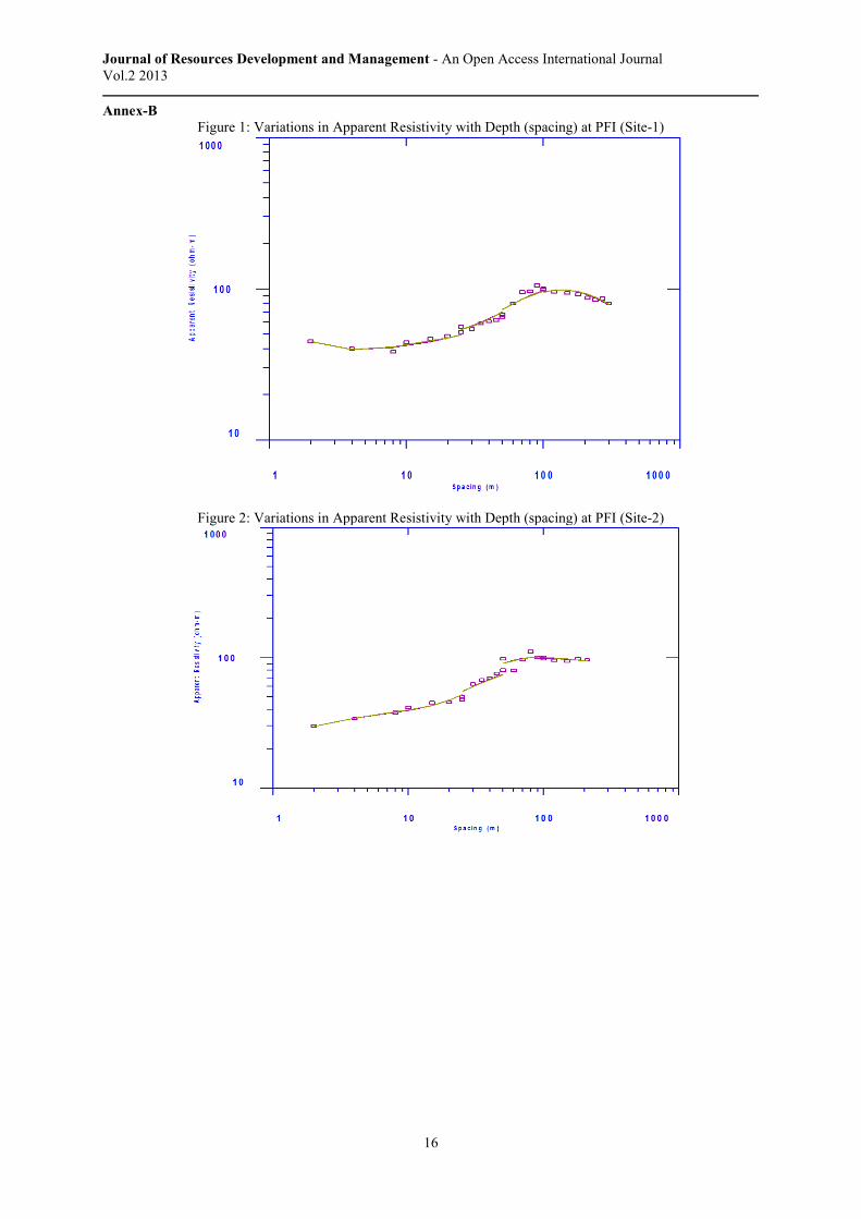
of the data shows that the surface materials at site 1(Annex-B figure 1) for the first layer of clay contents having

a thickness of 1.2 m to a depth of 1.2 m from a resistivity of 55 Ω-M. This layer was followed by boulder and

clay layer with thickness of 1.4 m to a depth of 2.6 m with a resistivity value of 32 Ω-M. The site 2 (Annex-B

figure 2) top layer was composed of boulder clay with a resistivity values of 32 Ω-M a thickness of 1 M to a

depth of 1 m. This is followed by sand and gravel in the second layer from a resistivity value of 58 Ω-M having

a total thickness of 14 m and depth of 15 m. The third layer identified at site 1 was sand and gravel with a

thickness of 26m to a depth of 29 m having resistivity value of 51Ω-M. hence this layer was a permeable one

and had a water bearing capability. At site two, the third layer had lateritic soil with a resistivity value of 310Ω-

M which has a thickness of 6 m upto a depth of 21 m. The last layer identified at site two was sand and gravel

with resistivity value of 88Ω-M, which was the water holding permeable layer. At site 1 the fourth layer


Vol.2 2013

13

identified was impermeable layer of lateritic soil with a resistivity value of 489Ω-M, having a thickness of 16 m

to a depth of 45 m. The last layer identified at site 1 was again a permeable layer of sand and gravel having a

thickness of 18 m to a depth of reaching to 64 m from resistivity value of 53 Ω-M. The water table estimated for

both these sites was 23 m. The estimated values of water table were also confirmed with respect to the existing

groundwater levels from the surroundings tubewells and they were found in good matching.

The University of Agriculture Sites

The second location selected for assessment was the University of Agriculture where two profiles were

surveyed. The data acquired was tabulated and preliminary analysis were carried out in the Microsoft excel were

then utilized for the detail analysis to be carried out in 1X1D. The relationships are given in annexure-B. The

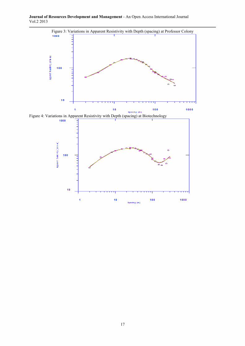
results show that at the professor colony (Annex-B figure 3) the upper most layer was lateritic soil with a

thickness of 1 m to a depth of 1 m with resistivity value of 740Ω-M. At biotechnology institute profile (annex-B

figure 4) first layer changed to clay contents for a resistivity value of 50Ω-M. The seepage to this regime from

surrounding irrigated agricultural land was observed. The second layer identified at Professor Colony was clay

contents for a resistivity value of 16Ω-M. The thickness of 38 m to a depth of 39 m was recorded. At

biotechnology institute the second layer was lateritic soil with a resistivity value of 631Ω-M having a thickness

of 7 m to a depth of 9 m. The third and fourth layers identified at Professor Colony were gravel materials which

were followed by sand and gravel for resistivity values of 142 and 29 Ω-M which give the thickness of 47 and 14

m. Respectively these layers reaches to the depth of 86 and 100 m. The groundwater at this location was

identified at depth of 41 m in the soil strata of gravel materials which is the best medium for groundwater

existence. However the next layer is sand and gravel which carries enormous amount of water. At biotechnology

the third and fourth layer identified were gravel and some mixture of clay contents. The fourth layer was sand

and gravel with resistivity values of 121 and 214 Ω-M. The thickness of these layers was 49 and 17 m, to the

depth of 83 and 100 m. The groundwater at this location was at a depth of 37 m in the medium of gravel and clay

contents. However the next layer to further depth was of sand and gravel which also carries water.

Hayatabad Sites

In Hayatabad two sites (1 & 2) were surveyed with set procedure details of which are given in annexure

(Annex-B figures 5 and 6). The analyses were carried out using 1X1D model. Results of the data showed that

the surface materials at site 1 were sand and clay with 2 m thickness and depth for the resistivity of 91Ω-M. The

second layer is sand stone with 3 m thickness to a depth of 5 m for resistivity value of 1215Ω-M. The third layer

identified was sand and clay having a thickness of 77 m to a depth of 82 m, from the resistivity value of 129Ω-M.

All these layers were dry and no moisture was observed in these layers. The last permeable layer identified was

sand and gravel with 14 m thickness to a depth of 96 m, for the resistivity value of 129Ω-M. This layer was

identified as water bearing layer so the water table identified at this location was at a depth of 92m. At site 2 the

surface materials were sand and gravel which were dried and no moisture was observed. The thickness of this

layer was 1 m to a depth of 1 m with a resistivity value of 189Ω-M. The second layer identified was sand and

clay which have thickness of 8 m to 9 m depth, the resistivity of this layer was 151Ω-M. The third layer

identified was a thick layer of boulder and clay with 4 m thickness to a depth of 13 m. The resistivity value of

this layer was 34Ω-M. The last and water bearing strata identified at this location was sand and gravel with 82 m

thickness to 95 m depth. The resistivity value of this layer was 166Ω-M. This layer was full of water as the

estimated value of groundwater table was also checked with existing water table depths in surroundings area

which were found in good agreement.

Conclusions

• The shallowest water table was at PFI site 1 & 2 were 23 m with respect to ground surface.

However the deepest water table estimated at Hayatabad, the most notable at site 1 which was

92 m with respect to ground surface. Whereas site 2 has a water table depth of 82 m with

respect to ground surface. The water bearing strata predicted at all of the locations was mostly

sandy clay, sand and gravel with some clay contents in small amount.

• Different types of subsurface strata were identified at various locations. However the dominant

strata throughout the study area was sand and gravel, sand stone, clay, sand stone and some

lateritic soil. Among the above mentioned strata the sand and gravel with clay was dominant in

University and PFI areas while in Hayatabad region sand and gravel with sand stone were

dominant.


Vol.2 2013

14

Table 1: Details of Strata Depth and thickness with Resistivities Values

S.NO Location Name of Layer Thickness of

Layer(m)

Depth of

Layer(m)

Resistivity of Layer(Ω-m)

1 PFI-Site 1 Clay 1.2 1.2 55

Boulder clay 1.4 2.6 32

Sand and Gravel 26 29 51

Lateritic Soil 16 45 489


2 PFI-Site 2 Boulder Clay 1 1 32


Lateritic soil 9 25 310


36 Professor

Colony

Lateritic soil 1 1 740

Clay 38 39 16

Gravel clay 47 86 142


4 Biotechnology Clay 1.5 1.5 50

Lateritic Soil 7 9 631

Clay 25 34 10

Grave Clay 49 83 121


19 Hayatabad Site

1

Sand and clay 2 2 91

Sand stone 3 5 1215


Sand and gravel 14 96 129

20 Hayatabad site

2



Boulder clay 4 13 34


References

Ahmad, M., Kutcher, G. P., 1992. Irrigation Planning with Environmental Considerations: A Case Study of

Pakistan's lndus Basin. Technical Paper 166. World Bank, Washington.

Anhtony, E., Voigt, Hans. J., Gnauck, R. N. H. A., Petzold, R. N. H., 2006. Groundwater Exploration and

Management using Geophysics: Northern Region of Ghana, Northern Ghana Natural

Resources Res. 15(2) 22.

Arshad, M., Sikandar, P., Baksh, A., Rana, T., 2007. The use of vertical electrical sounding resistivity method

for the location of low salinity groundwater for irrigation in Chaj and Rachna Doabs. Env

Earth Sci J. 60:1113–1129.

Bakhsh, A., Awan, Q. A., 2002. Water issues in Pakistan and their remedies. In: National Symposium on

Drought and Water Resources in Pakistan, 16th

March 2002, CEWRE, University of

Engineering and Technology Lahore, Pakistan 145-150.

Choudhury, K., Saha, D. K., Chakraborty, P., 2001. Geophysical study for saline water intrusion in a coastal

alluvial terrain, J. Appl. Geophys., 46: 189- 200.

EL-Waheidi, M. M., Merlanti, F., Pavan, M., 1992. Geoelectrical resistivity survey of the central part of Azraq

Basin (Jordan) for identifying saltwater/freshwater interface, J. Appl. Geophys. 29: 125-133.

Flathe, H., 1954. Possibilities and limitations in applying geoelectrical methods to hydrogeological problems in

the coastal areas of north-west Germany, Geophys. Prosp. 3:95–110.

Kaya, G. K., 2001. Investigation of groundwater contamination using electric and electromagnetic methods at an

open waste-disposal site: a case study from Isparta, Turkey, Environ. Geol. 40: 725-731.

Kelly, E. W., 1976. Geoelectric sounding for delineating ground water contamination, Ground Water, 14: 6-11.

Lashkaripour, G. R., 2003. An investigation of groundwater condition by geoelectrical resistivity method: A case

study in Korin aquifer, southeast Iran. Journal of Spatial Hydrology 3:1-5.

Meidav, T., 1960. An electrical resistivity survey for groundwater, Geophys. 25:1077–1093.

Niwas, S., Singhal, D. C., 1981. Estimation of aquifer transmissivity from Dar-Zarrouk parameters in porous

media. J. Hydrol., 50:393--399.

Onuoha. K. M., Mbazi, F. C. C.,. 1988. Aquifer transmissivity from electrical sounding data: the case of Ajali

Sandstone aquifers south-west of Enugu, Nigeria, in Ofoegbu, C.O., ED. Ground water and

mineral resources of Nigeria. Vieweg-Verlag. pp. 17–30.


Vol.2 2013

15

Oseji, J. O., Asokhia, M. B., Okolie, E. C., 2006. Determination of groundwater potential in obiaruku and

environs using surface geoelectric sounding. Springer Science+Business Media,

Environmentalist 26:301-308.

Oseji, J.O., Atakpo, E., Okolie, E.C., 2005. ‘Geoelectric Investigation of the Aquifer Characteristics and

Groundwater Potential in Kwale, Delta State, Nigeria’, Journal of Applied Science and

Environmental Management 9(1):157–1600.

Park, H. Y., Doh, S. J., Yun, S. T., 2007. Geoelectric resistivity sounding of riverside alluvial aquifer in an

agricultural area at Buyeo, Geum River watershed, Korea: an application to groundwater

contamination study. Environmental Geology. 53:849-859.

PES., 2009. Pakistan Economic Survey. Government of Pakistan, Finance Division, Economic Advisor’s Wing,

Isd.

Serres, Y. F., 1969. Resistivity prospecting in a United Nations groundwater project of Western Argentina,

Geophys Prosp 17: 449–467.

Soupios, P. M., Kouli, M., Valliantos, A. V., Stavroulakis, G., 2007. Estimation of aquifer hydraulic parameters

from surficial geophysical methods: A case study of Keritis Basin in Chania (Crete-Greece).

Journal of Hydrology. 338:122-131.

Tyson, A. N., 1993. ‘Georgia’s Groundwater Resources U.S Geological Survey Bulletin’. Pp. 1096:1-11.

Van Dam, J. C.. Meulenkamp, J. J., 1967. Some results of the geoelectrical resistivity method in groundwater

investigations in the Netherlands, Geophys Prosp. 15:92-115.

Vincenz, S. A., 1968. Resistivity investigations of limestone aquifers in Jamaica (Caribbean Groundwater

Karst), Geophys. 33:980-994.

WRI., 2001. World Resources People and Ecosystems: The fraying web of life, World Resources Institute ,

Washington DC.

Young, M. E., Debruijin, R. G. M., Salim AL-Ismaily, A., 1998. Exploration of an alluvial aquifer in Oman by

time-domain electromagnetic sounding, Hydrogeol. J. 6:383-393.

Zohdy, A. A. R., 1969. Application of deep electrical soundings for groundwater exploration in Hawaii,

Geophysics. 34:584-600.

Annex-A Table 1: Resistivity Values for Some Common Geological Formations (Anthony et al. 2006)

Material Nominal Resistivity (Ω-m)

Quartz 3 x 102– 10

6

Granite 3 x 102– 10

6

Granite (weathered) 30 – 500

Consolidated shale 20 – 2 x 103

Sandstones 200 – 5000

Sandstone(weathered) 50-200

Clays 1 – 102

Boulder clay 15 – 35

Clay (very dry) 50 – 150

Gravel (dry) 1400

Gravel (saturated) 100

Lateritic soil 120 – 750

Dry sandy soil 80 – 1050

Sand clay/clayed sand 30 – 215

Sand and gravel(saturated) 30 – 225

Mudstone 20-120

Siltstone 20-150

Journal of Resources Development and Management

Vol.2 2013

Annex-B

Figure 1: Variations in Apparent Resistivity with Depth (spacing) at PFI (Site

Figure 2: Variations in Apparent Resistivity with Depth (spacing) at PFI (Site


16

Variations in Apparent Resistivity with Depth (spacing) at PFI (Site

Variations in Apparent Resistivity with Depth (spacing) at PFI (Site

An Open Access International Journal

Variations in Apparent Resistivity with Depth (spacing) at PFI (Site-1)

Variations in Apparent Resistivity with Depth (spacing) at PFI (Site-2)

Journal of Resources Development and Management

Vol.2 2013

Figure 3: Variations in Apparent Resistivity with Depth (spacing) at

Figure 4: Variations in Apparent Resistivity with Depth (spacing) at Biotechnology


17

Variations in Apparent Resistivity with Depth (spacing) at Professor Colony

Variations in Apparent Resistivity with Depth (spacing) at Biotechnology

An Open Access International Journal

Professor Colony


Vol.2 2013

18

Figure 5: Variations in Apparent Resistivity with Depth (spacing) at Hayatabad site 1

Figure 6: Variations in Apparent Resistivity with Depth (spacing) at Hayatabad site 2


Vol.2 2013

19

Picture 1: Picture of the Instrument used for Data Acquisition

Picture 2: Instrument was being checked for Calibration


Vol.2 2013

20

Picture 3: No problem was observed during data collection at a temperature of 40C

o

groundwater investigation by using resistivity survey in

Documents