groundwater investigation and characterisation in …
TRANSCRIPT

GROUNDWATER INVESTIGATION AND CHARACTERISATION IN
MARIGAT AREA, BARINGO COUNTY, USING VERTICAL ELECTRICAL
SOUNDING RESISTIVITY SURVEYS
Cherop Komen Hezekiah
I56/CE/26608/2011
A thesis submitted in partial fulfillment of the requirements for the award of the degree of
Master of Science in the School of Pure and Applied Sciences of Kenyatta University
October, 2016

ii
DECLARATION
This thesis is my original work and has not been presented for award of a degree or any
other award in any university
Cherop Komen Hezekiah Signature Date
Department of Physics
Kenyatta University ...………………. ………………
P.O BOX 43844-00100
NAIROBI-KENYA
This thesis has been submitted with our approval as University Supervisors
Dr. Willis J. Ambusso Signature Date
Physics Department
Kenyatta University …….…………... ..………..……
P.O BOX 43844-00100
NAIROBI-KENYA
Dr. Githiri J. Gitonga Signature Date
Physics Department
Jomo Kenyatta University of Agriculture & Technology ……...…… ……………...
P.O BOX 6200
NAIROBI-KENYA

iii
DEDICATION
This thesis is dedicated to my wife Valarie

iv
ACKNOWLEDGEMENTS
I would like to sincerely thank the Almighty God for the care, knowledge, strength, hope
and patience He granted me during this Msc program.
My special thanks goes to my research supervisors Dr. W.J. Ambusso and Dr. J.G. Githiri
for their technical guidance, valuable and constructive advice during the planning and
development of this research work. I would like also to thank the chairman of the
department of physics, Dr. N.O. Hashim and the entire physics department lecturers for
their support and guidance.
Further, I wish to appreciate Baringo County Director of Water and Irrigation, Mr. J.R
Kiplagat and Superintendent Water engineer, Mr. D.K Kaitany for their technical advice
and guidance in this research work.
I am deeply indebted to my parents Mr. and Mrs. James Kibowen Cherop for giving me a
solid foundation in education and training me up in the right way. I must thank my
brother Joel Cherono for his hospitality and kindness in accommodating me during the
numerous trips I made to Nairobi.
To my fellow researchers, Mr. Seurey, Mr. Chirchir and Lucy Muchiri, I cannot but
appreciate the understanding and cooperation we displayed during field work amid
scorching sun, rugged terrain and scary thorns of Prosobis juliflora and cactus plants. To
all my colleagues in Geophysics class 2012, I say thank you.

v
TABLE OF CONTENTS
Content Page
DECLARATION .................................................................................................................. ii
DEDICATION ..................................................................................................................... iii
ACKNOWLEDGEMENTS ................................................................................................... iv
TABLE OF CONTENTS ........................................................................................................v
LIST OF TABLES ............................................................................................................... ix
LIST OF FIGURES ................................................................................................................x
LIST OF ABBREVIATIONS ............................................................................................... xii
ABSTRACT ....................................................................................................................... xiv
CHAPTER ONE .................................................................................................................... 1
INTRODUCTION .................................................................................................................. 1
1.1 Background to the study .................................................................................................... 1
1.2 Geological setting ............................................................................................................ 2
1.3 Statement of research problem .......................................................................................... 4
1.4 Objectives of the research project ...................................................................................... 5
1.4.1 General objective .......................................................................................................... 5
1.4.2 Specific objectives ........................................................................................................ 5
1.4.3 Rationale of the study .................................................................................................... 5
CHAPTER TWO ................................................................................................................... 6
LITERATURE REVIEW ....................................................................................................... 6
2.1 Resistivity of the earth materials ....................................................................................... 6
2.2 Resistivity method ............................................................................................................7
2.3 Groundwater exploration in Kenya .................................................................................... 9
2.4 Previous geophysical work in Marigat area .......................................................................10
CHAPTER THREE .............................................................................................................. 12

vi
THEORETICAL BACKGROUND ....................................................................................... 12
3.1 INTRODUCTION .......................................................................................................... 12
3.2 CURRENT FLOW IN THE GROUND ............................................................................ 13
3.2.1 Wenner configuration ................................................................................................... 14
3.2.2 Schlumberger configuration .......................................................................................... 15
3.3 Pumping Test .................................................................................................................. 17
3.3.1 Recovery Test method .................................................................................................. 17
CHAPTER FOUR ................................................................................................................ 21
MATERIALS AND METHODS ........................................................................................... 21
4.1 RESISTIVITY SURVEY ................................................................................................ 21
4.1.1 Introduction ................................................................................................................. 21
4.2 Field Instruments ............................................................................................................ 21
4.2.1 ABEM TERRAMETER SAS 1000/4000 ....................................................................... 21
4.2.2 Global Positioning System ........................................................................................... 23
4.3 Field Measurements ....................................................................................................... 24
4.4 Resistivity Data Processing ............................................................................................. 25
4.5 Parameter determination ................................................................................................. 26
4.5.1 Cumulative Resistivity method ..................................................................................... 26
4.5.2 Inverse modeling ......................................................................................................... 26
CHAPTER FIVE ................................................................................................................. 28
RESULTS AND DISCUSSION ........................................................................................... 28
5.1 Introduction ................................................................................................................... 28
5.1.1 VES and HEP Distributions ......................................................................................... 28
5.2 Interpretation of Resistivity data ..................................................................................... 29
5.2.1 Qualitative interpretation ............................................................................................. 29
5.2.1.1 Interpretation of Horizontal Electrical Profiles ............................................................ 29

vii
5.2.1.2 Interpretation of the apparent resistivity curves ........................................................... 30
5.2.1.3 Interpretation of cumulative resistivity curves............................................................. 32
5.2.2 Quantitative interpretation ........................................................................................... 33
5.2.2.1 Interpretation of Pseudo and Resistivity cross sections ................................................ 33
5.2.2.2 Models interpretation ................................................................................................ 36
5.3 Aquifer characteristics .................................................................................................... 53
5.3.1 Aquifer parameters of various soundings points in the study area.................................... 56
5.4 Discussion ..................................................................................................................... 59
CHAPTER SIX ................................................................................................................... 63
CONCLUSIONS AND RECOMMENDATIONS .................................................................. 63
6.1 Introduction ................................................................................................................... 63
6.2 Conclusions ................................................................................................................... 63
6.3 Recommendations .......................................................................................................... 65
REFERENCES ................................................................................................................... 66
APPENDIX I ...................................................................................................................... 70
SOUNDING POINTS AND THEIR COORDINATES .......................................................... 70
APPENDIX II ...................................................................................................................... 71
VES RAW DATA ................................................................................................................ 71
APPENDIX III .................................................................................................................... 74
HEP DATA ........................................................................................................................ 74
APPENDIX IV .................................................................................................................... 78
HEP GRAPHS .................................................................................................................... 78
APPENDIX V ..................................................................................................................... 79
CUMULATIVE RESISTIVITY CURVES ............................................................................ 79
APPENDIX VI ..................................................................................................................... 81
GRAPHS OF APPARENT RESISTIVITY VERSUS ELECTRODE SPACING ....................... 81

viii
APPENDIX VII .................................................................................................................. 82
AQUIFER PARAMETERS ................................................................................................. 82
APPENDIX VIII ................................................................................................................. 83
BOREHOLE DATA ............................................................................................................ 83
APPENDIX IX .................................................................................................................... 84
PUMPING TEST – DRAWDOWN MEASUREMENTS ....................................................... 84
APPENDIX X ..................................................................................................................... 88
PUMPING TEST – RECOVERY MEASUREMENTS .......................................................... 88

ix
LIST OF TABLES
Content Page Table 5.1: Borehole data of some drilled boreholes within the study area ....................... 53
Table 5.2: Aquifer parameters of various sounding points ............................................... 57
Table 5.3: Probable lithology of the study area .................................................................59
Table 5.4: Variation of groundwater temperature with depth .......................................... 61

x
LIST OF FIGURES
Content Page Figure 1.1: Geology of the Lake Baringo area ..................................................................... 3
Figure 2.1: Electrical resistivity and conductivity ranges of some rocks ........................... 6
Figure 3.1: The generalized form of electrical configuration used in resistivity .............. 13
Figure 3.2: Electrode configuration in Wenner array ....................................................... 14
Figure 3.3: Electrode configuration in Schlumberger array ............................................. 15
Figure 3.4: Drawdown measurements in recovery tests .................................................. 18
Figure 4.1: ABEM SAS TERRAMETER 1000/4000 ..................................................... 22
Figure 5.1: HEP and VES points in the study area .......................................................... 28
Figure 5.2: Graphs of HEP 1 and HEP 2 ........................................................................... 29
Figure 5.3: Graphs of apparent resistivity versus electrode spacing for HEP 1 ................ 31
Figure 5.4: Graphs of apparent resistivity versus electrode spacing for HEP 2 ................ 31
Figure 5.5: Cumulative resistivity curve of VES 1 ............................................................. 32
Figure 5.6a: Pseudo cross section and resistivity cross section of HEP 1 ......................... 34
Figure 5.6b: Pseudo cross section and resistivity cross section of HEP 2 ......................... 35
Figure 5.6c: Pseudo cross section and resistivity cross section of HEP 4 ......................... 35
Figure 5.6d: Pseudo cross section and resistivity cross section of HEP 5 ........................ 36
Figure 5.7a: VES 1 along profile 1 ..................................................................................... 38
Figure 5.7b: VES 2 along profile 1 ..................................................................................... 38
Figure 5.7c: VES 3 along profile 1 ................................................................................... 38
Figure 5.7d: VES 4 along profile 1 ..................................................................................... 39
Figure 5.7e: VES 17 along profile 1.................................................................................... 39
Figure 5.7f: VES 5 ............................................................................................................. 40
Figure 5.7g: VES 6 .......................................................................................................... 40

xi
Figure 5.7h: VES 7 along profile 3 ..................................................................................... 41
Figure 5.7i: VES 8 along profile 2 ..................................................................................... 42
Figure 5.7j: VES 9 along profile 2 ..................................................................................... 43
Figure 5.7k:VES 10 along profile 2 .................................................................................. 43
Figure 5.7l: VES 11 along profile 2 .................................................................................... 43
Figure 5.7m: VES 12 ......................................................................................................... 44
Figure 5.7n: VES 13 .......................................................................................................... 44
Figure 5.7o: VES 14 .........................................................................................................45
Figure 5.7p: VES 15 ...........................................................................................................45
Figure 5.7q: VES 16 .......................................................................................................... 46
Figure 5.7r: VES 18 along profile 4 .................................................................................... 47
Figure 5.7s: VES 19 along profile 4 ................................................................................. 48
Figure 5.7t: VES 20 along profile 4 ................................................................................... 48
Figure 5.7v: VES 22 along profile 4 .................................................................................. 49
Figure 5.7u: VES 21 ........................................................................................................... 50
Figure 5.7w: VES 23 ........................................................................................................ 50
Figure 5.7x: VES 24 along profile 5 ................................................................................... 51
Figure 5.7y: VES 25 along profile 5 ....................................................................................52
Figure 5.7z: VES 26 along profile 5 ....................................................................................52
Figure 5.8: Graphs of residual drawdown against time ratio for Salabani .......................54
Figure 5.9: Graphs of residual drawdown against time ratio for Endao-Barkibi ............. 55
Figure 5.10: Aquifer transmissivity map ......................................................................... 58
Figure 5.11: Aquifer depth map ........................................................................................ 58
Figure 5.12: Graph of Temperature against Depth for Salabani borehole ....................... 62

xii
LIST OF ABBREVIATIONS
IP Induced Polarization
DC Direct Current
UN United Nations
VES Vertical Electrical Sounding
HEP Horizontal Electrical Profile
SAS Signal Averaging System
GPS Global Positioning System
RTI Radar Technologies International
AAF Amsha Africa Foundation
GIS Geographic Information System
GDC Geothermal Development Company
CDN Catholic Diocese of Nakuru
CCF Christian Children’s Fund
LPM Litres Per Minute
WSL Water Struck Level
WRL Water Rest Level
DBP Distance Between Points
WRMA Water Resource Management Authority
GWTS Groundwater and Technical Service Limited
JICA Japan International Cooperation Agency
MoWD Ministry of Water Development
WAAS Wide Area Augmentation System

xiii
KenGen Kenya electricity Generating company
UNESCO United Nations Educational, Scientific and Cultural
Organization

xiv
ABSTRACT
Marigat area, located in Baringo-Bogoria basin is a semi-arid part of the eastern Rift
valley experiencing limited supply of potable water. Groundwater in this region is
unexploited due to challenges of undefined nature of fault lines and presence of
underground geysers. This study was carried out with the aim of investigating the
groundwater potential and to characterise water bearing formation in Marigat area,
Baringo County using resistivity method. Vertical electrical sounding (VES) method was
applied using Schlumberger electrode configuration to determine the vertical variation of
resistivity with depth and to delineate probable aquifers that can be developed into
productive boreholes. A total of 28 VES points were probed along five Horizontal
Electrical Profiles (HEP) within an area of about 19.2 km2 using an ABEM SAS
terrameter 1000/4000. The collected data was analysed using IP2WIN software and
Surfer 8 Golden software which revealed the presence of 3-6 interpretable geoelectric
layers which were categorized into three inhomogeneous formations corresponding to the
existing borehole data within the study area. The first formation is an unsaturated top
alluvial deposit with resistivity ranging from 2.49 m to 258 m and thickness ranging
from 0.284 m to 44.1 m. The second formation which is slightly weathered and fractured
rock has resistivity varying from 0.77 m to 71.5 m while the thickness varies from
4.33 m to 63.2 m. The third formation is characterized by fresh and weathered basement
of compact basaltic rock with resistivity values varying from 0.0685 m to 6979 m
and thickness ranging from 25.1 m to 52.1 m. Two of the soundings were carried out near
existing boreholes in which pumping tests had been carried out. Dar Zarrouk parameters
were computed and used to estimate the aquifer hydrologic properties. It was found that
the transmissivity values obtained range between 13.569 m2/day – 1429.052 m2/day
while the geothermal gradient determined using Salabani borehole data (C6362) was
found to be 239.730C/km. The results of this study shows that groundwater potentials
along the sedimentary basin is good for development at shallow depths ranging between
35 m – 50 m located at the mid-central and the stretch towards south east of the study
area while the basement rock with low resistivity values and high geothermal gradient is
good for geothermal exploration. Based on the geological setting and the resistivity
results of this study, it is highly recommended that chemical analysis for potable
groundwater should be carried out after drilling in order to ascertain on its quality.

1
CHAPTER ONE
INTRODUCTION
1.1 Background to the study
Groundwater is a very important component of water resources in nature. It is a hidden
treasure stored in subsurface void spaces and moves slowly through geologic formations
of soil and rocks called aquifers. Several geophysical methods can be used to investigate
groundwater resources and the success of each method depends on the geological and
hydrological system (Palmasson, 1975). However, not all geophysical methods are
appropriate for groundwater exploration. For deep groundwater exploration, seismic
reflection and magnetotellurics have proven to be successful while the integrated use of
gravity and magnetic methods are good for reconnaissance surveys to solve complicated
geological, hydrological and environmental problems. Goldman and Neubauer, (1994)
noted that electrical technique is the most popular geophysical method used in shallow
groundwater exploration due to the close relationship between electrical conductivity and
the hydrogeological properties of the aquifer. Electrical resistivity methods were
developed in early 1900’s and they have been used extensively for ground water
investigation by many workers (Olurunfemi and Fasuy, 1993). It is considered to be the
most suitable method for groundwater investigation and characterisation in most
geological occurrence due to simplicity of technique. This study was therefore
undertaken to investigate depth, thickness and distribution of water bearing formation

2
using Geophysical electrical resistivity method in order to characterize the groundwater
potential and to advise individuals and the county in groundwater development.
1.2 Geological setting
Marigat area is located within the eastern floor of the Kenya Rift Valley as shown in
figure 1.1. The area lies between lake Baringo to the north and Lake Bogoria to the south.
It is delineated by longitude E'50350 to E'00360 and latitude N'2000 to N'3500 . The
region is a semi-arid part of Rift valley floor with numerous wetland systems that have
been formed along lake shorelines and faults where hot, warm and cold springs have
developed.
The Marigat floor is covered by Quaternary deposits which include the lacustrine silts of
Loboi plain which were formed in the last phase of development of the original lake
Baringo-Hannington before it dwindled to form Lake Baringo and Lake Bogoria. These
Quaternary deposits form the main water bearing strata that are apparently unaffected by
faulting and are characterized by almost total lack of boulders and pebbles (Walsh, 1969).
The recent alluviums that include fluvial and alluvial deposits form part of the dominant
geology of the mid- central in the study area as shown in figure 1.1. Important succession
of Quaternary alluvium sediments occurs in the region and some of the sedimentary units
contain abundant fossils and intermittent evidence of hominid activity as explained by
Chapman et al. (1978). These alluviums are hydrogeologically important since they are
likely to form alluvial aquifers that could yield productive boreholes in the sedimentary
basin. The northern part of Marigat consists of Kapthurin beds which are grid faulted and
overlie the Lake Hannington phonolites that are presumed to constitute a coarse boulder

3
torrent-wash with subordinate silts and volcanic tuffs containing oogonia (female
reproductive structure of algae). Roure et al. (2009) inferred that the presence of oogonia
in the Kapthurin formation tufa (chemically formed sedimentary rock) suggests that the
water depths are moderate and generally quiet, alkaline and that low energy conditions
prevailed.
The Chemeron beds are found in the North western part of the study area and they consist
of series of tuffs, tuffaceous earths and silts with subordinate diatomite. These beds
overlie the Kwaibus basalts which are purplish, non-porphyritic rock with large drawn-
out vesicles, often lined with yellow zeolites (Walsh, 1969).
Figure 1.1: Geology of the Lake Baringo area in the Eastern (Gregory) Rift, Kenya
(adapted from Chapman and Brook, 1978)

4
1.3 Statement of research problem
The major source of water for purpose of life is surface water which is correspondingly
becoming inadequate due to unpredictable weather patterns and climate change globally.
Groundwater is an essential substitute to surface water, however, this resource is hidden
and its occurrence and distribution depends on the regional geology and hydrogeologic
setting. Groundwater in Marigat area is unexploited and efforts by organizations and
individuals to sink boreholes in this region have not been very successful due to
challenges of undefined nature of fault lines in the rift valley, presence of underground
geysers and lack of detailed hydro geophysical information of the area. Several
geophysical measurements that include magnetotellurics, transient electromagnetic and
seismics have been used successfully to study deep geothermal resources that are located
tens of kilometers below the subsurface, however, these techniques penetrate deeper and
distort the shallow formations that are likely to bear water. This study was therefore
necessary to be undertaken in this area using electrical resistivity survey in order to
investigate and characterise the shallow groundwater potentials which will further help to
delineate aquifers that could be developed into productive boreholes and reduce the risks
of drilling dry boreholes. The immediate benefits of the groundwater will greatly improve
the economic activities in this area and create job opportunities in agricultural and
industrial sectors hence steering our county towards realization of vision 2030.

5
1.4 Objectives of the research project
1.4.1 General objective
The main objective of this study is to investigate groundwater potentials and groundwater
characterization in Marigat area, Baringo County using Electrical resistivity method.
1.4.2 Specific objectives
The specific objectives of the study are:
i. To conduct ground resistivity survey of Marigat area using Vertical Electrical
sounding (VES).
ii. To generate 2D cross-sections along the profiles on discerned aquifer location.
iii. To estimate the depth and thickness of the aquifers in the study area.
iv. To determine the aquifer hydraulic parameters and characterise its potential in
Marigat area.
1.4.3 Rationale of the study
Electrical resistivity method is an effective technique for defining geoelectric properties
of the subsurface formation due to its close relationship with electrical conductivity and
hydrogeological properties of the underlying rocks. The field procedures are simple, less
costly and its application with vertical electrical sounding provides accurate information
on groundwater potentials and aquifer characteristics within the study area. The
information on groundwater constitutes a knowledge base which is fundamental to water
resource assessment and ground water development for domestic and industrial use.

6
CHAPTER TWO
LITERATURE REVIEW
2.1 Resistivity of the earth materials
The most useful parameters used in describing the earth’s materials and formations are
the electrical properties. This is because the variations in electrical resistivity typically
correlate with variations in water saturation, fluid conductivity, porosity, permeability
and the presence of waste material (Geo2X, 2012). Depending on the site, these
variations may be used to locate the depth of water table and aquifer identification, buried
structures, contaminant plumes, saline intrusion, stratigraphic units and any other
structure whose electrical properties contrast with the surrounding materials. Figure 2.1
below shows a representative chart illustrating how the resistivities of important rock
groups compare to each other (Palacky, 1987). Generally, the true resistivity of earth
material is dependent upon composition, grain size, water content and other physical
characteristics.
Figure 2.1: Electrical resistivity and conductivity ranges of some rocks (adapted from
Palacky, 1987)

7
Fine grained materials have lower resistivities than coarse-grained materials while
unweathered and unfractured hard rocks such as lithified sedimentary rocks, volcanic
rocks, plutonic rocks and some metamorphic rocks generally have high resistivity values.
The presence of fracturing and weathering lowers the resistivity of the rocks (Hasbrouck
and Morgan, 2003). The occurrence of groundwater greatly reduces the resistivity of all
rocks and sedimentary materials through electrolytic conduction. Because of this effect,
groundwater may be explored using electrical and electromagnetic geophysical methods.
2.2 Resistivity method
The main geophysical methods that are employed in groundwater exploration include
electrical method, electromagnetic method, seismic method, magnetic method and
gravity method. Of all the surface exploration techniques, electrical resistivity method is
the most commonly used techniques to delineate aquifer composition, groundwater,
bedrock, and fresh and salt zones (Robinson and Coruh, 1988; Burger, 1992; Telford et
al., 1990).
Vertical electrical sounding has been used to determine zones with high yield potential
in Mangalore block, Tamil Nadu, India (Ahilan and Kumar, 2011). It was found that,
prominent low resistivity anomalies indicated weaker zones which represent a
prospective zone for groundwater development while high resistivity anomalies
indicated poorly weathered massive rock. Majumdar and Das (2011) carried out
hydrological characterisation and estimation of aquifer properties from electrical
sounding data in Sagar Island Region, India, and observed that vertical electrical
sounding (VES) delineates the top soil, the saline water zone, brackish ground water

8
zones, impermeable clay layer and freshwater aquifer in subsurface geological
formation. This is mainly because the resistivity method is dependent on parameters
such as temperature, porosity and fluid salinity. Resistivity methods have been used to
locate vertical and horizontal fracture zones in East Africa (Drury et al., 2001). It was
found that volcanic rocks form important aquifer systems in the region. However,
locating deep horizontal fracture zones such as the boundary between lava flows can be
difficult.
Direct current resistivity method is the common tool for groundwater exploration in arid
areas. Nejad et al. (2011) carried out resistivity survey technique to explore groundwater
in arid region of Curin basin of southern Iran and the quantitative interpretation of the
VES curves led to the determination of the aquifer boundaries. Resistivity method can be
used alongside other geophysical methods in areas of complex geology and
hydrogeology to evaluate groundwater conditions and find potential aquifer zones.
Bayode and Akpoarebe (2011) used magnetic and electrical resistivity methods to
investigate a spring in Ibuji, Southwestern Nigeria. They found that a major vertical
discontinuity within basement bedrock which they suspected to be a major fault line was
the spring source and that the spring was structurally controlled. Ekstrom et al. (1996)
used DC resistivity imaging and ground penetrating radar (GPR) to investigate the extent
and different zones within an aquifer in river alluvium in SW Zimbabwe. Tsiboah (2002)
carried out resistivity and time-domain electromagnetic methods in Delamare Farm,
North of Lake Naivasha, Kenya. The two methods were used in order to complement
one another and to enhance the interpretation of the subsurface information in terms of
conductivity for aquifer mapping.

9
2.3 Groundwater exploration in Kenya
Groundwater investigations in Kenya has been done by several govermental
organizations and private companies which include Water Resource Management
Authority (WRMA), Groundwater and Technical Services Limited (GWTS), Radar
Technologies International (RTI), Japan International Cooperation Agency (JICA)
among others. Groundwater exploration was done in the year 2013 in Turkana, Kenya.
The investigation was done by Radar Technologies International (RTI), during the
course of a survey of groundwater conducted for the Kenyan government on behalf of
UN. The aquifers were detected with WATEX system, RTI’s state-of-the-art, space
based exploration technology, that prospects and explores subsurface water, soils and
geology by processing multi-frequency and multi-polarization radar imagery in shallow
aquifers and integrating the WATEX base imagery with geophysical data interpretation
such as magnetic, resistivity, gravity and seismic data for deep aquifers (Landsat
Science, 2013). The two aquifers; Lotikipi basin aquifer and the Lodwar basin aquifer
were identified using advanced satellite exploration technology. The existence was then
confirmed by drilling conducted by UNESCO. It was found that Turkana which is
characterized by large expanses of unexplored hydrogeological territory hosts a
minimum reserve of 250 billion cubic meters despite the fact that it is located in a semi-
arid region.
Amsha Africa Foundation (AAF) (2011), carried out Resistivity survey in Mwatate,
Singila-Majengo, in an attempt to locate a freshwater reservoir after a previous drilling
attempt at a nearby site drew saline water. Vertical electrical sounding curve

10
interpretations using RES1D geophysical software depicted prospective safe water
aquifer at a depth of 40 m - 60 m. Jӧrgen and Ingemar (2005), in a minor field study
carried out a GIS-mapping of groundwater in Nakuru and Baringo districts and observed
that the bedrock in Nakuru - Baringo districts consists of fluoride bearing minerals
which contaminate the water and high levels are more common in deeply drilled
boreholes than in the surface water. This information corroborates with JICA (2011) on
groundwater assessment in Baringo County.
2.4 Previous geophysical work in Marigat area
Groundwater exploration in Marigat area was first done in 1970’s. Pencol (1984) carried
out some geophysical work in Marigat area and the results indicated that there may be
groundwater at shallow depth in old sand and gravel filled channel to the south of
Kathiorin river and to the west of the new Marigat - Nginyang road. A seismic and
gravity survey (Swain, 1981) covered the area between Lake Baringo and Kerio-valley
and between Lake Baringo and Lake Turkana to the north. The purpose of this survey
was to study the deep geological structures beneath the crust in the rift floor. The seismic
data collected near Marigat indicated that the recent sediments near the lakes are very
thick. It is estimated that the thickness of the sediments could exceed one kilometre to the
south of the lake.
In 1987, a team from ministry of water development, Nakuru office conducted resistivity
soundings at Salabani, Ngambo, Eldume and Logumukum. The objective of the
measurements was to locate sites for boreholes in the area between Lake Bogoria and
Lake Baringo. The study revealed very low values of resistivity of about 5 Ohms which

11
indicated the presence of clay layers or saline water. However, no drilling was done at
that time and thus correlation between the sounding and lithology was not done (MoWD,
1987).
The ministry of Energy of Kenya in a reconnaissance study for geothermal potential in
the area carried out Schlumberger resistivity measurements in Lake Baringo area; the
northern parts of Marigat area (Mariita and Kilele, 1989). The analysis of the soundings
carried out in that area indicated a discrete anomaly less than 20 m at depths of 1000 m
lodged northwest of Lake Baringo. The field data obtained was later built on by KenGen
(Mungania et al., 2004) in an attempt to describe Lake Baringo geothermal prospect.
Simiyu et al. (2011) also observed that geophysical surveys particularly resistivity,
gravity, magnetic and seismic methods had been carried out in the past in the geothermal
areas in the Lake Baringo and Bogoria geothermal prospects. Little has been documented
on geophysical groundwater exploration and some of the work has been carried out by
Water Resource Management Authority (WRMA), Catholic Diocese of Nakuru (CDN),
(Jӧrgen and Ingemar, 2005), and Non-Governmental Organizations (NGOs) which
include Christian Children’s Fund (CCF) and the World Vision. Some of the drilled
boreholes and the driller’s logs in Marigat area are shown in appendix VI and they reveal
presence of shallow ground water potentials having higher than ambient temperatures
with some recording up to 400C (Simiyu et al., 2011). This study therefore, investigated
groundwater potentials and characterisation of the shallow subsurface formation using
vertical electrical sounding resistivity techniques in order to deduce the potentiality of the
groundwater resource for economic exploitation.

12
CHAPTER THREE
THEORETICAL BACKGROUND
3.1 INTRODUCTION
The electrical resistivity method is one of the most used techniques in groundwater
exploration. This is because rock resistivity is sensitive to its water content and also the
resistivity of water is very sensitive to its ionic content. This implies that resistivity
method is able to map different stratigraphic units in a geological section as long as the
units have a resistivity contrast. Porosity is also a major control of resistivity in rocks.
This is because the pore spaces between the rock particles determines the rate at which
groundwater flows within the aquifer as described by Archie’s equation (3.1) below.
N
t
wm
wR
RaS
1
(3.1)
where, wS is water saturation, is porosity, wR is formation water resistivity, tR is
observed bulk resistivity, a , m and N are empirical constants. Other factors which
influence the resistivity of rocks are the size of particles and the mobility of ions in water
which decreases with temperature and ceases when water is frozen to ice (Scollar et al.,
1990).
Electrical resistivity surveying is based on the principle that the distribution of electrical
potential in the ground around a current-carrying electrode depends on the electrical
resistivities and distribution of the surrounding soils and rocks (ABEM instruction
manual, 2010). In this method, electrical direct current (DC) is applied between two

13
electrodes implanted in the ground and measuring the potential difference between the
two potential electrodes.
3.2 CURRENT FLOW IN THE GROUND
Electrical currents are carried by moving charged particles. Current flow through soil or
sediments is entirely carried by ions created when salt crystals in the ground dissociate
in the presence of soil water (Campana and Piro, 2008). The resistance in a single
electrode (point source) of hemispherical shell of radius r which is found between a
perfect insulator and a semi-infinite isotropic, homogeneous conductor of resistivity ρ is
given by the equation (3.2);
22 r
dxR
(3.2)
where 22 r is the surface area of the hemispherical shell. The current flows radially
away from the electrode so that the current distribution is uniform over hemispherical
shells centered on the source. The circuit is completed by current sink at a large distance
from the electrode as shown in figure 3.1 below:
Figure 3.1: The generalized form of Electrical configuration used in resistivity
measurements.
B C
rA rB
A D
∆V
RB RA
+I -I

14
Braja (2010) observed that when the subsurface inhomogeneities exist, resistivity will
vary with relative positions of electrodes. Therefore, the computed of apparent
resistivity will be given by equation 3.3 below.
BABA
a
RRrrI
V
1111
2
(3.3)
3.2.1 Wenner configuration
This method is used in determining the lateral variation in resistivity. The current and
potential electrodes are maintained at a fixed separation and are progressively moved
along a profile. It is normally employed when a rapid survey of an area is desired. The
Wenner array consists of four collinear, equally spaced electrodes with electrode spacing
a. The outer two electrodes A, B are typically the current (source) electrodes as shown
in Figure 3.2 below and the inner two electrodes M, N are the potential (receiver)
electrodes. The array spacing expands about the array midpoint while maintaining an
equivalent spacing between each electrode.
Figure 3.2: Electrode configuration in Wenner array (Zohdy et al., 1990)

15
Substituting the values of electrode spacing of Wenner array in equation (3.3) yields
equation (3.4);
(3.4)
where a is the apparent resistivity, a2 is the geometric factor (K), V is the potential
difference and I is the electric current.
3.2.2 Schlumberger configuration
Schlumberger configuration is used in vertical electrical sounding. The potential
electrodes M and N are installed at the centre of the electrode array with a small
separation (a), typically less than one fifth of the spacing between the current electrodes
A and B as shown in figure 3.3 below. The electrodes A and B are increased to a greater
separation (L) during the survey while M and N remain in the same position until the
observed voltage becomes too small to measure.
Figure 3.3: Electrode configuration in Schlumberger array (Zohdy et al., 1990)
From equation (3.4) the apparent resistivity can be written as shown in equation (3.5);
I
VKa
(3.5)
where K is the geometric factor expressed as in equation (3.6);
I
Vaa
2

16
MN
MNAB
K
22
22
(3.6)
Substituting the values of electrode spacing of Schlumberger array in equation (3.6)
yields equation (3.7);
44
2 a
a
LK (3.7)
Replacing equation (3.7) in equation (3.5) we obtain an equation of apparent resistivity
for Schlumberger configuration expressed as equation (3.8);
(3.8)
The general solution for the potential at any given layer is defined in cylindrical
coordinates since the electrical fields have cylindrical symmetry with respect to vertical
line through the current source. According to Koefoed (1970) the potential )(rV can be
expressed as in equation (3.9);
drJhzDhzC
IzrV iiiii )()(sinh)()(cosh)(
2),( 0
0
1
(3.9)
where )(0 rJ is the Bessel function of order zero
is a variable of integration (roots)
1 is the resistivity of the first layer.
ih is the depth of the thi layer.
r is the radial distance from the current source.
44
2 a
a
L
I
Va
17
z is the depth below the surface.
At the surface where 0z , the potential at the surface resulting from any number of
horizontal layers is derived by solution of Laplace’s equation given by equation (3.10);
drJK
IrV )()(
2)( 0
0
1
(3.10)
where )(K is the Kernel function and it is controlled by the thickness and resistivities
of the underlying layers.
3.3 Pumping Test
3.3.1 Recovery Test method
This is one the methods of determining well performance and efficiency. It is conducted
after pumping has stopped to estimate the aquifer transmissivity. When pumping is
stopped, water level rises towards its pre-pumping level. The resulting drawdown at any
time after pumping stops is algebraic sum of drawdowns from well and buildup from
imaginary well.

18
Figure 3.4: Drawdown measurements in Recovery test (Ghafour, 2005)
The Residual drawdown 'S is given by Jacob and Cooper equation shown in (3.11);
'ln
4'
t
t
T
QS
(3.11)
The plot of residual drawdown )'(S versus the logarithm of 't
t forms a straight line with
the gradient expressed as in equation (3.12);
T
QS
4
303.2' (3.12)
So that transmissivity (T) is written as shown in equation (3.13);
'4
303.2
S
QT
(3.13)
The combination of thickness and resistivity into single variables in other words known
as Dar Zarrouk parameters are used as basis for the evaluation of aquifer properties. The
concept of Dar Zarrouk parameters was first introduced by Mailet (1974) to explain the
problem of non- uniqueness in the interpretation of resistivity depth sounding curves. Dar

19
Zarrouk parameters consist of the transverse resistance RT and longitudinal conductance
LC. MacDonald et al. (1999) suggested that depending on the geological conditions,
transmissivity can be directly related to Dar Zarrouk parameters. Therefore, for a
horizontal, homogenous and isotropic layer, the transverse resistance RT (Ωm2) is defined
as:
hRT (3.14)
The longitudinal conductance LC (mho) is defined as:
hh
LC (3.15)
Where h is the thickness of the layer in metres and is the electrical resistivity of the
layer in ohm-metres and is conductivity of the layer.
Aquifer transmissivity T (the product of aquifer thickness and hydraulic conductivity) is
related to the hydraulic conductivity K and the aquifer thickness h as shown in equation
(3.16);
KhT (3.16)
Combining equations (3.14), (3.15) and (3.16) yields equation (3.17);
C
TT L
KRKR
KT (3.17)
In areas of similar geologic setting and water quality, the product K remains fairly
constant (Niwas and Singhal 1981). Therefore, equation (3.17) can be expressed as
shown in equation (3.18);
AK (3.18)

20
The constant A (Siemen/day) is calculated from the pumping test results and it is possible
to determine transmissivity and its variation from place to place including those areas
where borehole pumping tests data are not available provided one knows the K value
from the existing borehole pumping test data and from the interpreted resistivity
measurements of the aquifer.

21
CHAPTER FOUR
MATERIALS AND METHODS
4.1 RESISTIVITY SURVEY
4.1.1 Introduction
Resistivity measurements were made in the northern parts of Marigat area, referred to as
Southern Baringo Zone (Mungania et al., 2004) in Baringo Bogoria basin in the month of
April, 2014. The survey covered an area of approximately 19.2 km2, and consisted of 5
profiles and 28 vertical electrical sounding (VES) points. Wenner electrode array was
conducted in each profile while four electrode Schlumberger array was chosen for
vertical electrical sounding survey. The prolific growth of Prosobis juliflora (Mathenge)
in the study area limited accessibility, thus, each profile and sounding point was selected
based on accessibility and applicability of the method in the study area. Electrical
resistivity survey technique with application of horizontal profiling and vertical electrical
sounding were applied to investigate the shallow basement structures which include
dykes, faults and fracture zones that are likely to be conduits and reservoirs to
groundwater.
4.2 Field Instruments
4.2.1 ABEM TERRAMETER SAS 1000/4000
For resistivity survey the most commonly used device is ABEM terrameter shown in
figure 4.1. Terrameter SAS 1000/4000 is a light-weight, compact and cost efficient
instrument. It is a versatile geophysical tool suitable for a broad range of applications

22
ranging from groundwater and mineral exploration to infrastructure site investigations. It
has a built in PC compatible microcomputers which can save up to 1,000,000 data points
on the internal flash disk. It is also fast and highly time-efficient data acquisition with
precision and accuracy better than 1% over whole temperature range (ABEM instruction
manual, 2010).
Figure 4.1: ABEM SAS TERRAMETER 1000/4000
ABEM SAS 1000/4000 operates in three modes:
i. Resistivity survey mode: It comprises a battery powered, deep-penetrating
resistivity meter with output sufficient for a current electrode separation of 2000
meters under good surveying condition and apparent resistivity ranging from 0.05
milliohms to 1999 kilo ohms.
ii. Induced polarization (IP) mode: It measures the transient voltage decay in a
number of time intervals. The induced polarization effect is measured in terms of
chargeability.

23
iii. Voltage measuring mode: It comprises a self-potential instrument that measures
natural DC potentials. The result is displayed in volts or millivolts.
One of the important advantages of ABEM SAS 1000/4000 terrameter is its ability to
measure in four channels simultaneously. The electrically isolated transmitter sends out
well-defined and regulated signal currents with strength up to 1000mA and a voltage up
to 400V (limited by the output power 100W). The receiver discriminates noise and
measures voltages correlated with transmitted signal current (resistivity surveying mode
and IP mode) and also measures uncorrelated DC potentials with the same discrimination
and noise rejection (voltage measuring mode). The microprocessor monitors and controls
operations and calculated results. Another advantage of SAS 1000/4000 is its ability to
distinguish between geological formations with identical resistivity e.g. clay and water.
This is applicable in induced polarization mode since SAS 1000/4000 permits natural or
induced signals to be measured at extremely low levels with excellent penetration and
low power consumption.
4.2.2 Global Positioning System
Global positioning system (GPS) is a satellite-based navigation system that provides
information on location and time of a place anywhere on or near the earth surface. All
GPS satellites synchronize operations so that the repeating signals are transmitted at the
same instants. The signals, moving at the speed of light arrive at a GPS receiver at
slightly different times because some satellites are further away from the receiver than
others. The distance to the GPS satellites can be determined by estimating the amount of
time it takes for their signals to reach the receiver. The receiver then estimates the

24
distance to at least four GPS satellites and calculates its position in terms of latitude,
longitude and altitude.
4.3 Field Measurements
The site reconnaissance was conducted first in the study area then the sounding points
were chosen based on the accessibility and applicability of the method in the study area.
For aquifers that were likely to be located in fault fracture zones, Horizontal electrical
profiling was first conducted at probable sites in order to know the exact location of the
faults, then followed by vertical electrical sounding at each promising point to obtain
geological profiling data in depth. For aquifers of sedimentary layers, the geophysical
survey involved conducting VESs directly at promising sites in the study area. Wenner
array was used Horizontal electrical profiling to determine the horizontal or lateral
variation of resistivity. The spacing between successive electrodes remained constant and
all electrodes which were collinear were moved for each reading. Five resistivity profiles
of length 1300m, 1240m, 260m, 1250m and 740m were measured. The profiles in the
study area had different lengths due to inaccessibility of some parts caused by the prolific
growth of Prosobis juliflora (Mathenge), cactus plants and the rugged terrain.
Vertical electrical sounding (VES) with the commonly used Schlumberger configuration
was used for the purpose of determining the vertical variation of resistivity. The current
and potential electrodes were maintained at the same relative spacing and the whole
spread was progressively expanded about a fixed central point (Kearey and Brooks,
1984). The electrodes were placed along a straight line as shown in Figure 3.3 with 2
AB

25
and 2
MN spacing ranging between 1.6 m to 250 m and 0.5m to 25 m respectively and
MNAB 5 .
4.4 Resistivity Data Processing
The collected data in the study area were processed so as to prepare the dataset for
interpretation. Horizontal Electrical Profile survey data were used to select points where
vertical electrical sounding was conducted. Regions where low resistivity values were
observed were selected as VES points as shown in Figure 5.2 and Appendix IV since they
are attributed to weak zones which are likely to be faults that are conduits to
groundwater. The VES data was input into the computer and curves were plotted using
IP 2WIN software (version 3.0.1) developed by the Geophysics Group Moscow State
University for inverse interpretation. The field resistivity structures of sounding data were
determined digitally based on the type of electrical configuration used and gave
information on true resistivity, number of layers, depth and thickness of geological
formation at each sounding point as shown in figure 5.7a to figure 5.7z. The VES data
from several soundings along the profiles were merged to form pseudo cross sections and
resistivity cross sections which are full two-dimensional geoelectric layers describing the
lateral variation of resistivity of the geoelectric structures and formations (Loke and
Barker, 1996)

26
4.5 Parameter determination
4.5.1 Cumulative Resistivity method
The graphs of cumulative sums of apparent resistivities against the values of half
electrode spacing are called cumulative resistivity curves. In this method, the calculated
cumulative resistivities are plotted against the Schlumberger electrode spacing of some
VES points along the profiles. An abrupt change in slope of the curves indicates a change
in the electrical properties at a depth equal to electrode spacing. This method is useful in
determining the approximate depth, thickness of the hydrogeologic cross–section at each
sounding points and the type of the apparent resistivity curves based on the constant
increments of depth.
4.5.2 Inverse modeling
The standard linearized inversion approach to solving the non-linear inverse problems are
largely based on iterative processes. Menke (1984) noted that this processes involves
conversion of polar distance 2
AB to equivalent depth as well as updating the model
parameters at each step to best fit the observed data using damped least-squares as shown
in equation (4.1);
m (GTG+2 I)
1GT d (4.1)
where m is the parameter correction vector, d is the data difference vector, G is the
Jacobian matrix, I is the identity matrix and the term is called the damping factor
which is a scalar quantity that controls both the speed of convergence and resolution. The
Jacobian matrix contains the partial derivatives of the model responses which are

27
computed at each iteration and approximated by finite differences with respect to the
model parameters. The choice of is critical thus a product of the misfit error and an
estimate of a cut-off eigenvalue )( is used (Narayan et al., 1994). The trace of GGT is
used to calculate the average eigenvalue and it obtained by dividing the trace by the
number of layer parameters (N) as shown in equation (4.2);
N
Traceav (4.2)
The equation (4.2) gives a damping factor which is written as equation (4.3);
avf (4.3)
where is rms error and f is a fraction of the average eigenvalue.

28
CHAPTER FIVE
RESULTS AND DISCUSSION
5.1 Introduction
5.1.1 VES and HEP Distributions
The ground resistivity survey was taken along five profiles as shown in figure 5.1 below
oriented in the N-S, NE-SW and E-W directions normal to the regional features such as
faults and rivers.
Figure 5.1: HEP and VES points in the study area
VES 1
VES 2
VES 3
VES 4
VES 5 VES 6
VES 7
VES 8
VES 9
VES 10
VES 11
VES 12
VES 13
VES 14 VES 15VES 16
VES 17
VES 18
VES 19VES 20
VES 21
VES 22
VES 23
VES 24
VES 25
VES 26
Salabani borehole
Silonga borehole
Endao borehole
Endao-Barkibi borehole
35.965 35.97 35.975 35.98 35.985 35.99 35.995 36 36.005 36.01
LONGITUDE
0.51
0.514
0.518
0.522
0.526
0.53
0.534
LA
TIT
UD
E
HEP 1
HEP 2
HEP 3
HEP 4
HEP 5
N
0 0.01 0.02 0.03 0.04DEGREES

29
5.2 Interpretation of Resistivity data
5.2.1 Qualitative interpretation
This refers to the interpretation of Hummel’s cumulative resistivity curves, electrical
profiles, resistivity pseudo cross-sections and comparison of the relative changes in the
apparent resistivity and thickness of the detected layer on the sounding curves. This gives
information about the number of layers, their continuity through the area and reflects the
degree of homogeneity or heterogeneity of an individual layer.
5.2.1.1 Interpretation of Horizontal Electrical Profiles
The graphs in figure 5.2 below shows the lateral variation of resistivity across HEP 1 and
HEP 2. Horizontal electrical profile 1 had varying resistivity values lying between 12.72
Ωm to 45.88 Ωm while HEP 2 had resistivity values lying between 11.03 Ωm and 35.53
Ωm.
Figure 5.2: Graphs of Horizontal electrical profiles of HEP 1 and HEP 2.

30
Five points with low resistivity values were selected for vertical electrical sounding
(VES) in HEP 1 while four points were selected in HEP 2 based on accessibility and
applicability of vertical electrical sounding method in the study area. Horizontal electrical
profile 3 shown in appendix IV is the shortest profile in the study area with one vertical
electrical sounding point (VES 7). This is attributed to the inaccessibility of the area
caused by rugged terrain and the dense growth of Prosobis Juliflora (Mathenge).
Horizontal electrical profile 4 and HEP 5 had generally low resistivity values ranging
from 10.34 Ωm to 26.68 Ωm. From the two profiles, three VES points were selected from
each profile for probing which are VES 19, VES 20, VES 22 and VES 24, VES 25, VES
26 respectively. The Low resistivity anomalies seen in the profiles are interpreted as
shallow bedrock formations, fractured zones and faults that are likely to be water bearing
layers and conduits to groundwater. These sites with low resistivity values were selected
for vertical electrical sounding in order to describe in detail the vertical variation of
resistivity with depth.
5.2.1.2 Interpretation of the apparent resistivity curves
The shapes of the field curves were observed qualitatively to get an idea on the number of
layers and the resistivity of the layers by using partial curve matching technique and
Hummel’s cumulative method. It was observed that the dominant type of curve was of K-
type indicating presences of three layers followed by combination of curves that include
Q, KH, QK, KK and KA indicating three to six subsurface medium as shown in figure
5.3, figure 5.4 and appendix VI. This implies that the dominant parameter controlling the
shape of the K-shaped sounding curve is the transverse resistance since the middle of the

31
three layers is of higher resistance while low resistivity values are observed at depth
below 100 m in most of the sounding points.
Figure 5.3: Graph of apparent resistivity versus electrode spacing for HEP 1
Figure 5.4: Graph of apparent resistivity versus electrode spacing for HEP 2
0
10
20
30
40
50
60
1 10 100 1000
AP
PA
RE
NT
RE
SIS
TIV
ITY
(oh
m.m
)
AB/2 (m)
VES 1
VES 2
VES 3
VES 4
VES 17
0
10
20
30
40
50
60
70
80
1 10 100 1000
AP
PA
RE
NT
RE
SIS
TIV
ITY
(o
hm
.m)
AB/2 (m)
VES 8
VES 9
VES 10
VES 11

32
5.2.1.3 Interpretation of cumulative resistivity curves
The abrupt change in the slope of the cumulative resistivity curve shown in figure 5.5
revealed presence of three geoelectric layers of varying resistivities and thickness. These
multi-layered formations consist of different earth materials with the first layer consisting
of unsaturated top soil. The second layer consists of weathered formation while the third
layer comprise of fractured basement which has low resistivity values.
Figure 5.5: cumulative resistivity curve of VES 1
0 100 200 300 400 500
300
250
200
150
100
50
0
0 100 200 300 400 500
300
250
200
150
100
50
0
AB
/2 (
m)
CUMULATIVE RESISTIVITY (ohm-m)

33
5.2.2 Quantitative interpretation
The main objective of quantitative interpretation is to obtain the geoelectric parameters
and geoelectric sections in order to clearly define and characterise the aquifers. This was
done by analyzing the collected data using IP2 WIN software and relating the acquired
model parameters such as the true resistivity values with the existing geological
information and lithological logs of the drilled boreholes shown in appendix VIII.
5.2.2.1 Interpretation of Pseudo and Resistivity cross sections
The pseudo cross-sections and resistivity cross-sections shown in figure 5.6a to figure
5.6d shows the orientation of the lateral variation of resistivity with depth along the
profiles. They provide the information on the formation of the earth material that aids in
its characterisation. The initial model estimates were input into IP 2WIN software to
generate the pseudo cross sections and resistivity cross sections from interpolated VES
data along the profiles using inversion techniques.
The pseudo cross section along profile one shows relatively low resistivity less than
15Ωm on top layer across VESs 1, 2, 4 and 17 which corresponds to alluvium deposits
and moist volcanic soils. The resistivity values increase with depth up to 50m and
decreases uniformly to a depth of about 200m. This indicates that a more conductive
medium exists at a depth of about 50m and below which is likely to be highly weathered
and fractured tuffs that are aquiferous. Across VES3 and VES4, there is a high resistive
layer from a depth of 10m to 40m. This layer is likely to be dry volcanic soils and
tuffaceous materials that are not aquiferous. The pseudo cross-section along profile 2, 4
and 5 shows relatively high resistivity above 25 Ωm and decreases uniformly with depth.

34
The top highly resistive layer corresponds to dry top superficial of volcanic deposits and
running sand spreading to a depth of about 10 m. The low resistivity values in pseudo
cross-section 2 and 5 corresponds to highly weathered and fractured basalts while in
pseudo cross-section 4 it correlates with weathered phonolites and hard basalts which are
aquiferous. The resistivity cross-sections show the geoelectrical layers that indicate the
rock strata of the geological formations in the study area. The cross sections have varying
resistivity values with depth indicating different layers of the rock strata across the
profile. The geoelectrical layers are interpreted quantitatively in order to delineate the
rock type which is bearing water.
Figure 5.6a: Pseudo cross section and Resistivity cross-section of HEP 1 showing spatial
distribution of layer structures across VES 1, VES 2, VES 3, VES 4 and VES 17.
35
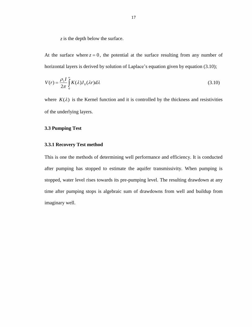
Figure 5.6b: Pseudo cross section and Resistivity cross-section of HEP 2 showing spatial
distribution of layer structures across VES 8, VES 9, VES 10 and VES 11.
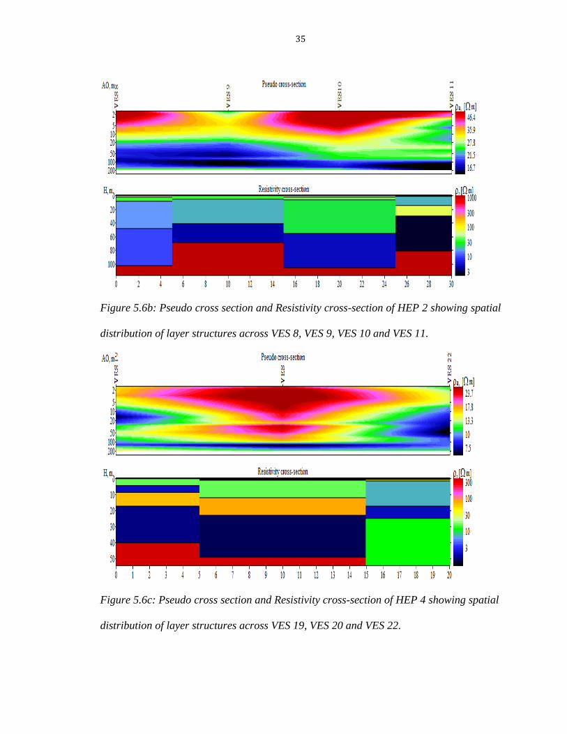
Figure 5.6c: Pseudo cross section and Resistivity cross-section of HEP 4 showing spatial
distribution of layer structures across VES 19, VES 20 and VES 22.

36
Figure 5.6d: Pseudo cross section and Resistivity cross-section of HEP 5 showing spatial
distribution of layer structures across VES 24, VES 25 and VES 26.
5.2.2.2 Models interpretation
The lithologic formation from productive boreholes in conjunction with the knowledge of
the local geology in Marigat area was used as constraints in interpretation of the models
obtained from the vertical electrical sounding curves. The VES curves have varying
geoelectric parameters; number of layers (N), resistivity (ρ), thickness (h), depth (d) and
altitude (alt).The red and black curve give the information of the relation between 2
AB
and apparent resistivity value. The blue curve gives information about the resistivity
value variation while the open dots are the apparent resistivity values. The model
parameters of the VESs along HEP 1 are shown in figure 5.7a to figure 5.7e. In VES 1,
the first layer has thickness of 0.676 m which corresponds to dry top superficial deposits

37
of alluvium followed by dry volcanic soils of resistivity 163 Ωm. Beneath the dry
volcanic soils lie tuffs and tuffaceous materials which are highly weathered with
resistivity of 21.1 Ωm and thickness ranging between 19.3 m - 71.1 m below the ground
surface and resistivity of 7.85 Ωm. In VES 2, moist volcanic soils of resistivity 19.9 Ωm
overlie the superficial deposits of sand and gravels while at a depth of 43.2 m to 84.2 m
lies highly weathered and fractured tuffs with low resistivity of 2.16 Ωm sitting on
weathered basalt of resistivity 385 Ωm. VES 3 revealed six geoelectric layers with
different resistivity values. The first layer is composed of sand and gravel with thickness
of 0.617 m and resistivity of 58.3 Ωm. The second layer consists of alluvial sediments
followed by compact dry volcanic soils of resistivity 208 Ωm with thickness ranging
between 4.2 m – 10.9 m. The fourth and fifth layers with resistivity of 7.08 Ωm and 30.2
Ωm are composed of slightly weathered tuffs and tuffaceous materials between 10.9 m –
89.8 m where shallow to deep aquifers are expected. Highly weathered and fractured
tuffs with resistivity 0.129 Ωm are expected below 89.8 m. This layer is highly
conductive and the low resistivity value is interpreted as geothermal fluid.
VES 4 and VES 17 revealed 4 geoelectric layers consisting of alluvium deposits in the
first layer followed by moist to dry volcanic soils and slightly weathered tuffs in the
second and third layers respectively. The fourth layer in VES 4 and VES 17 represents an
aquiferous basement consisting of highly weathered and fracture basalts below 76.7 m in
VES 4 and highly weathered and fractured tuffs below 36.3 m in VES 17.

38
Figure 5.7a: VES 1 along the Profile 1(RMS =6.07%)
Figure 5.7b: VES 2 along profile 1(RMS =7.26%)
Figure 5.7c: VES 3 along profile 1(RMS =3.84%)

39
Figure 5.7d: VES 4 along profile 1(RMS = 8%)
Figure 5.7e: VES 17 along profile 1(RMS = 6.03%)
VES 5 and VES 6 shown in figure 5.7f and figure 5.7g were taken along Chemeron basin
located on the slopes of Tugen hills and they revealed the presence of four geoelectric
layers with relatively similar geological formation. The first layer consists of dry layer of
alluvial deposits followed by fractured moist layer of volcanic soil with resistivity of 12.7
Ωm and 19.8 Ωm in VES 5 and VES 6 respectively. The third layers are aquiferous
consisting of weathered basalts of resistivity 2.98 Ωm and 1.3 Ωm and thickness ranging
between 42.2 m – 70.2 m and 44.3 m – 74.5 m in VES 5 and VES 6 respectively. The
fourth layers represent hard basement of basalts with resistivity of 1292 Ωm in VES 5
and 740 Ωm in VES 6. Shallow aquifers are expected in the second layers while deep
aquifers are expected in the third layers and the fourth layers act as the confining bed.

40
Figure 5.7f: VES 5 (RMS= 9.93%)
Figure 5.7g: VES 6 (RMS= 9.3%)
VES 7 shown in figure 5.7h was selected along HEP 3 and it revealed five geoelectric
layers. The top layer consists of dry superficial deposits of sand and gravels with
resistivity of 8.24 Ωm followed by a thin layer of dry volcanic soils with resistivity of
190 Ωm and thickness ranging between 0.516 m – 0.979 m lying on top of slightly
fractured trachytes and basalts with resistivity of 23.6 Ωm and thickness ranging between
0.979 m – 26 m. The fourth layer is very conductive with low resistivity of 3.49 Ωm and
thickness ranging between 26 m- 44.6 m and it composed of weathered basalt grits and
silts. The fifth layer has very high resistivity values of 6979 Ωm below 44.6 m and this
layer is described as fresh basement of compact basalts acting as the confining bed.

41
Figure 5.7.h: VES 7 (RMS= 9.97%)
The figure 5.7i to figure 5.7l shows the results of VES 8, VES 9, VES 10 and VES 11
taken along HEP 2 reveal the presence of five geoelectric layers. These layers are top soil
(clayey and sandy), dry to moist volcanic soils, slightly weathered basalts, highly
weathered and fractured basalts and fresh basement of compact basalts. VES 8 revealed
dry volcanic soils of depth 1.58 m and resistivity of 64.8 Ωm in the first layer followed
by dry to moist volcanic soils with resistivity of 34.6 Ωm and thickness ranging between
1.58 m - 8.25 m. The third layer is composed of slightly weathered basalts of resistivity
18.4 Ωm and thickness ranging between 8.25 m – 48.1 m where shallow aquifers are
expected. Below this layer is a probable unconfined aquifer which is composed of highly
weathered and fractured basalts with resistivity of 10 Ωm and thickness ranging between
48.1 m – 102 m. Fresh basement of compact basalts is expected in the fifth layer with
resistivity of 2555 Ωm below 102 m. This layer is hard rock and potable water in not
expected below this depth.
In VES 9, a thin layer of top superficial deposits of resistivity 11.3 Ωm lie on top of moist
volcanic soils of resistivity 38.7 Ωm and thickness within a range of 0.37 m - 4.9 m. The
third layer consists of slightly weathered basalts of resistivity 18.7 Ωm and thickness

42
ranging between 4.9 m - 41.2 m in which shallow aquifers are expected. The fourth layer
is an aquiferous layer of highly weathered and fractured basalts with resistivity and
thickness of 4.85 Ωm and 41.2 m - 68 m lying on top of fresh basement of compact
basalts. VES 10 consists of dry to moist volcanic soils in the first two layers followed by
slightly weathered basalts containing shallow aquifers of thickness ranging between 5.92
m - 55.3 m and resistivity of 28.4 Ωm. This layer is underlain by highly weathered and
fractured basalts with resistivity of 6.25 Ωm and thickness ranging between 55.3 m – 105
m. This layer is aquiferous and it overlies fresh basement of compact basalts with
resistivity of 1542 Ωm and indefinite thickness since it is the last layer. VES 11 has
almost the same geological formation as VES 10, except that the third layer consists of
dry volcanic soils of resistivity 75.6 Ωm and thickness between 14.7 m and 29.3 m. The
aquiferous layer lies between 29.3 m and 80.8 m and it is composed of highly weathered
and fractured basalts of resistivity of 3.23 Ωm lying on top of fresh basement of compact
basalts of resistivity 1398 Ωm.
Figure 5.7i: VES 8 along profile 2 (RMS= 3.4%)

43
Figure 5.7j: VES 9 along profile 2 (RMS= 8.94%)
Figure 5.7k: VES 10 along profile 2 (RMS= 2.67%)
Figure 5.7l: VES 11 along profile 2 (RMS= 7.21%)
VES 12 and VES 13 consist of 5 geoelectric layers as shown in figure 5.7m and figure
5.7n. In VES 12, the first geoelectric layer is the topsoil formation comprising of dry
sandy clay with some silts with thickness and resistivity of 0.301m and 12.6 Ωm
respectively. Beneath this layer is dry volcanic soils followed by compact dry volcanic
soils of resistivity 80.5 Ωm and thickness ranging between 13 m - 25.8 m which act as
confining layer. The fourth layer consists of highly weathered and fractured tuffs with

44
resistivity of 1.23 Ωm and thickness ranging between 25.8 m – 53.4 m lying above
slightly weathered basalts of resistivity 263 Ωm. VES 13 has the first layer comprising of
dry top soil formation of resistivity 258 Ωm followed by moist layer of volcanic soils
with resistivity and thickness of 12.5 Ωm and 0.28 m – 11.4 m respectively. The third
layer is a confining layer of dry volcanic soils with resistivity of 71.5 Ωm lying above
highly weathered and fractured tuffs with resistivity 1.92 Ωm and thickness ranging
between 23.7 m and 59.5 m. Below this layer is slightly weathered basalts with resistivity
of 540 Ωm hence VES 12 and VES 13 forms a confined aquifer between 23.7 m– 59.5 m.
Figure 5.7m: VES 12 (RMS= 7.8%)
Figure 5.7n: VES 13 (RMS= 6.08%)
VES 14 and VES 15 are shown in figure 5.7o and figure 5.7p. VES 14 revealed 5
geoelectric layers as shown in figure 5.7o. The first geoelectric layer, which is the topsoil
formation, is composed of alluvial deposits with some silt having a thickness of 8.79 m

45
and resistivity of 34 Ωm. The second and third geoelectric layer consists of weathered
and fractured tuffs where shallow aquifers are expected. The fourth layer contains highly
weathered and fractured tuffs with low resistivity of 2.17 Ωm and thickness ranging
between 44.2 m – 94.5 m and below this layer is slightly weathered basalts of resistivity
151 Ωm. In VES 15, the first geoelectric layer constitutes dry superficial deposits which
include alluvium and silts which overlie a thin layer of dry volcanic soils with resistivity
and thickness of 128 Ωm and 3.55 m – 5.87 m respectively. The third layer is expected to
provide shallow aquifers and it consists of moist to highly weathered and fractured
basalts ranging between 5.87 m and 53.2 m and resistivity of 17.3 Ωm. The fourth layer
is an aquiferous having resistivity and thickness of 2.99 Ωm and 53.2 m - 90.5 m.
Figure 5.7o: VES 14 (RMS= 2.8%)
Figure 5.7p: VES 15 (RMS= 4.88%)
Figure 5.7q shows the results of VES 16. VES16 and VES 3 revealed relatively the same
geological formation with six geoelectric layers. The top layer comprises of superficial

46
deposits of sandy clay soil followed by alluvial sediments lying on compact dry volcanic
soils with resistivity of 132 Ωm and thickness ranging between 4.36 m and 9.87 m. The
fourth and the fifth layers are composed of weathered and fractured tuffs that are the
aquiferous with resistivity ranging between 4.34 Ωm and 41.1 Ωm. The sixth layer is
very conductive with low resistivity of 0.069 Ωm which is described as geothermal fluid
located below 57.9 m.
Figure 5.7q: VES 16 (RMS= 3.71%)
VES 18 shown in figure 5.7r is composed of five geoelectric layers. The top layer
consists of superficial deposits of thin layer of sandy clay soil of resistivity 79.5 Ωm and
thickness 1.24 m followed by a thin layer of alluvial sediments of resistivity 19.9 Ωm and
thickness ranging between 1.24 m to 9.72 m. Sticky clay is expected in the third layer
with resistivity of 5.45 Ωm and thickness ranging between 9.72 m and 16.6 m. This layer
is not a good prospect for groundwater exploration since it contains clay and its
derivatives. The fourth layer is the aquiferous layer composed of slightly weathered
tuffaceous materials of resistivity 49.8 Ωm overlying highly weathered basement of
fractured tuffs.

47
Figure 5.7r: VES 18 along profile 4 (RMS= 7.32%)
VESs 19, 20 and 22 shown in figure 5.7s to figure 5.7v were carried out along HEP 3
which lies along Silonga borehole. VES 19 consists of 5 geoelectric layers with the first
layer comprising of loose brownish soils having a resistivity of 16.9 Ωm and thickness of
4.25 m. The second layer is composed of sticky clay with resistivity of 2.49 Ωm and
thickness ranging between 4.25 m and 8.4 m. This layer overlies alluvial deposits of
resistivity 64.4 Ωm which act as a confining layer with thickness ranging between 8.4 m -
17 m. The fourth layer is an aquiferous layer with resistivity of 1.72 Ωm and thickness
ranging between 17 m - 40.1 m lying on fresh basement of basaltic rock with high
resistivity of 921 Ωm which is likely to act as a confining bed to the aquifer.
In VES 20, six geoelectric layers are expected with the first thin layer comprising of
loose brownish soils followed by basaltic boulders with resistivity of 162 Ωm and
thickness ranging between 0.592 m – 1.14 m. The third layer with resistivity of 16 Ωm
and thickness ranging between 1.14 m – 12.1 m is composed of dry to moist volcanic
soils lying on top of alluvial deposits with resistivity of 79.2 Ωm and thickness ranging
between 12.1 m and 22.6 m which may act as a confining layer. The fourth layer is the

48
aquiferous layer with low resistivity of 1.4 Ωm and thickness ranging between 22.6 m –
48.9 m lying on top of a confining bed of hard basaltic rock with resistivity of 440 Ωm.
VES 22 was carried out on the eastern part of Silonga borehole and revealed five
geoelectric layers consisting of top layer of loose brownish soils lying on top of alluvial
deposits with resistivity of 43.5 Ωm. The third and fourth layers consist of sticky sand
clay and sticky clay with low resistivity of 8.04 Ωm and 2.45 Ωm respectively. These are
not good aquiferous layers since they contain clay and their derivatives. The fifth layer is
an aquiferous layer composed of highly fractured phonolites with old land surfaces and
resistivity of 13.2 Ωm below 27.4 m.
Figure 5.7s: VES 19 along profile 4 (RMS= 6.85%)
Figure 5.7t: VES 20 along profile 4 (RMS= 9.1%)

49
Figure 5.7v: VES 22 along profile 4 (RMS= 4.61%)
The results of VES 21 and VES 23 are shown in figure 5.7u and figure 5.7w. The top
layer in VES 21 consists of thin layer of sand clay followed by dry volcanic soils lying on
hard abrasive basalts of resistivity and thickness 55.6 Ωm and 4.28 m - 36.6 m
respectively. The fourth layer is an aquiferous layer which consists of highly fractured
phonolites with OLS of resistivity 2.65 Ωm and thickness ranging between 36.6 m – 97.4
m. Slightly weathered basalts of resistivity 242 Ωm lie beneath this layer and act as the
confining bed. The first layer in VES 23 is a thin layer of sandy clay soils lying on top of
running river sands with resistivity of 16.6 Ωm and thickness ranging between 0.295 m -
9.34 m. The third layer is an aquiferous layer of slightly weathered basalts with resistivity
of 5.19 Ωm and thickness ranging between 9.34 m – 40.3 m. The fourth layer is hard
abrasive basalts with resistivity of 60 Ωm and thickness 40.3 -72.1 m lying on top of
highly weathered basalts which is likely to be a rock bearing saline water having low
resistivity of 0.222 Ωm at a depth of 72.1 m.

50
Figure 5.7u: VES 21 (RMS= 2.19%)
Figure 5.7w: VES 23 (RMS= 9.72%)
VESs 24, 25 and 26 shown in figure 5.7x to figure 5.7z were taken along HEP 5 and it
shows remarkable geologic features based on the resistivity distribution of the rock layers
with depth. VES 24 and VES 25 consists of an overlying layer of running river sands
which spreads across the profile followed by sticky sand clay of resistivity 9.28 Ωm and
5.31 Ωm and thickness between 1.78 m – 12.2 m and 3.09 m -6.74 m respectively. This is
presumably underlain by hard abrasive basalts which act as a confining layer to a highly
weathered and fractured basaltic rock of resistivity 1.44 Ωm at a depth ranging between
24.2 m – 52.5 m and 14.4 m – 36.5 m in VES 24 and VES 25 respectively. The fifth layer

51
is hard basaltic rock which is slightly weathered with resistivity of 364 Ωm and 433 Ωm
and it acts as the confining bed.
VES 26 consists of 6 geoelectric layers. The first layer with resistivity of 72.4 Ωm and
thickness of 1.14 m corresponds to running river sands followed by rounded boulders
with resistivity of 27.2 Ωm which overlie sticky clay with resistivity and thickness of
6.35 Ωm and 7.75 m – 12.1 m respectively. The fourth layer with depth ranging from
12.1 to 26.4 m and resistivity of 71.4 Ωm correspond to hard abrasive basalt which act as
the confining layer that overly a highly weathered and fractured basaltic rock with
resistivity 1.15 Ωm and thickness ranging between 26.4 m – 51.6 m. This layer represents
a confined aquifer which underlies hard basaltic rock of resistivity 499 Ωm and depth
below 51.6 Ωm.
Figure 5.7x: VES 24 along profile 5 (RMS= 8.44%)

52
Figure 5.7y: VES 25 along profile 5 (RMS= 9.28%)
Figure 5.7z: VES 26 along profile 5 (RMS= 9.62%)

53
5.3 Aquifer characteristics
There are five boreholes within and around the study area. The borehole data and aquifer
parameters for four boreholes which were available are tabulated below:
Table 5.1: Borehole data of some drilled boreholes in the study area
BOREHO
LE
NAME
LOCATION:
GRID
RERENCE
BOREHOLE
SERIAL NO.
TOTAL
DEPTH
(m)
WSL
(m)
WRL
(m)
Q
(m3/hr)
PWL
(m)
DRAW
DOWN
(m)
Salabani
36000.511'E;
00031.885'N C-15060 50 38;45 33.7
2.7 36 2.31
Silonga
360 00.405’E ;
00031.041’N - 44 28;34 36.2
3.6 39.14 2.94
Kampi-
Turkana
350 59.476’E ;
00028.336’N C-15286 56 42;44 18
2.88 48.36 20.34
Endao-
Barkibi
35057.626'E ;
00031.383'N C-15066 81
52;70-
75 59.8
2 72.4 12.64
RANGE 44 – 81 28 - 75 18 – 59.8
2 – 3.6 36-72.4
2.31–
20.34
Borehole data obtained from Kabarnet Water Resource Management Authority (October,
2013)
From the data of the analysed boreholes in table 5.1 above, the boreholes exploit aquifers
between 28-75 m depth. When correlated with driller’s logs in Appendix VIII, it is noted
that these aquifers lie within the highly weathered basalts in Salabani and Endao-Barkibi,
fractured phonolites in Silonga and weathered sediments in Kampi-Turkana. These
boreholes have discharge rates that range between 2 m3/hr and 3.6 m3/hr and drawdown
ranging between 2.31 m and 20.34 m which represents good yield (WRMA, 2013).
The pumping test results for two boreholes were obtained from WRMA Kabarnet as
shown in appendix IX and appendix X. The values of the time ratio
't
t and residual
drawdown 'S from the recovery test for Salabani borehole and Endao-Barkibi were
used to draw the residual drawdown graphs and the following graphs were obtained:

54
Figure 5.8: Graph of Residual drawdown against time ratio for Salabani Borehole
The linear fit for residual drawdown per log cycle on linearized scales is obtained using
equation (5.1) as shown below.
Y = A + B *(X) (5.1)
Parameter Value Error
------------------------------------------------------------
A -0.13148 0.01223
B 0.41174 0.01067
Therefore, the slope represented by B correspond to 'S which is the residual drawdown
per log cycle of 't
t. Thus, 41174.0' S .
From table 5.1 the value of the borehole discharge is hmQ /7.2 3 .
Replacing 'S and Q in equation (3.13) yields transmissivity (T) as shown in equation
(5.2);
1 10 100 1000
0.0
0.4
0.8
1.2
1.6
2.0
1 10 100 1000
0.0
0.4
0.8
1.2
1.6
2.0
Re
sid
ua
l d
raw
do
wn
(m
)
Time ratio (t/t')

55
41174.04
7.2303.2
T 0311.02018.1 hm /2 (5.2)
The transmissivity (T) of an aquifer is related to its hydraulic conductivity (K) as shown
in equation (5.3);
KbT b
TK (5.3)
where, b is the aquifer thickness. For Salabani Borehole which is a weathered basalt
mb 8 as shown in Appendix VIII. Therefore, 0039.01502.08
2018.1K hrm /
or 0936.0605.3 K daym /
The residual drawdown graph for Endao-Barkibi is shown in figure 5.9 below:
Figure 5.9: Graph of Residual drawdown against time ratio for Endao-Barkibi borehole.
10 100 1000
2
4
6
8
10
12
10 100 1000
2
4
6
8
10
12
Re
sid
ua
l d
raw
do
wn
(m
)
Time ratio (t/t')

56
From the graph in figure 5.9 the linear fit for residual drawdown per log cycle on
linearized scales is as shown below,
Parameter Value Error
------------------------------------------------------------
A 2.05295 0.04232
B 1.17853 0.04527
------------------------------------------------------------
Similarly, the slope represented by B corresponds to 17853.1' S and the discharge is
hmQ /2 3 . Substituting these values in equation (3.13) yields the transmissivity (T)
shown in equation (5.4);
17853.14
2303.2
T 31101.0 0162.0 hm /2 (5.4)
For Endao-Barkibi borehole which is a hard basaltic rock the thickness mb 8 as shown
in Appendix VIII. Therefore the hydraulic conductivity K is given by
03888.08
31101.0K 002.0 hrm / or 933.0K 048.0 daym /
5.3.1 Aquifer parameters of various soundings points in the study area.
To calculate the area aquifer parameters, pumping test data of Salabani borehole and
Endao-Barkibi that have penetrated the productive aquifers in the eastern and the western
part of the study area were used to calculate the aquifer transmissivity (T) and hydraulic
conductivity (K). The average value of the constant A was calculated using equation
(3.18) and the results are tabulated in table 5.2. These results were used in determination
of other aquifer parameters within the study area where vertical electrical sounding was
conducted. The transmissivity map was drawn as shown in figure 5.10 with values
ranging between 13.569 m2/day and 1429.052 m2/day.

57
Table 5.2: Aquifer parameters of various sounding points
VES
No.
Aqui
fer
thick
ness
(m)
True
Resistiv
ity
(Ωm)
Transvers
e
Resistance
(RT) (Ωm2)
Hydraulic
Conductivi
ty
from
pump- test
(m/day)
A =K/ρ Calculated
transmissivi
ty
T=ART
(m2/day)
Calculated
Hydraulic
conductivi
ty
(m/day)
Aquife
r
Depth
(m)
1 51.7 7.85 405.85 323.621 6.260 71.1
2 41 2.16 88.56 70.618 1.722 84.2
3 52.1 30.20 1573.42 1254.645 24.081 89.8
4 63.2 21.30 1346.16 1073.428 16.985 76.7
5 28 2.98 83.44 66.535 2.376 70.2
6 30.2 1.30 39.26 31.306 1.037 74.5
7 18.6 3.49 64.91 51.762 2.783 44.6
Endao-
Barkibi
30.4 6.11 185.74 0.933 0.1527
±
0.0079
148.112 4.872 81
8 53.8 10.00 538.00 429.001 7.974 102
9 26.8 4.85 129.98 103.646 3.867 68
10 49.4 6.25 308.75 246.197 4.984 105
11 51.5 3.23 166.35 132.644 2.576 80.8
12 27.6 1.23 33.95 27.070 0.981 53.4
13 35.8 1.92 68.74 54.810 1.531 59.5
14 50.2 2.17 108.93 86.864 1.730 94.5
15 37.3 2.99 111.53 88.932 2.384 90.5
16 36.4 41.10 1496.04 1192.942 32.773 57.9
17 29.3 11.20 328.16 261.675 8.931 36.3
18 27 49.8 1344.60 1072.184 39.711 43.6
19 23.1 1.72 39.73 31.682 1.372 40.1
20 26.3 1.40 36.82 29.360 1.116 48.9
21 60.7 2.65 160.86 128.266 2.113 97.4
22 7.55 13.20 99.66 79.469 10.526 24.7
23 31 5.19 160.89 128.294 4.139 72.1
SALA
BANI
30.5 2.60 79.30 3.605 1.442 ±
0.0359
60.802 1.994 50
24 28.3 1.44 40.75 32.496 1.148 52.5
25 22.1 0.77 17.02 13.569 0.614 36.5
26 25.1 71.40 1792.14 1429.052 56.934 51.6
A(average)=0.7974
±0.0219

58
Figure 5.10: Aquifer transmissivity map of the study area
Figure 5.11: Aquifer depth map of the study area
35.965 35.97 35.975 35.98 35.985 35.99 35.995 36 36.005 36.01
Latitude
0.51
0.515
0.52
0.525
0.53
0.535
Lo
ng
itu
de
0 0.01 0.02 0.03 0.04
0
100
200
300
400
500
600
700
800
900
1000
1100
1200
1300
1400
Transmissivity
N
Degrees
35.965 35.97 35.975 35.98 35.985 35.99 35.995 36 36.005 36.01
Latitude
0.51
0.515
0.52
0.525
0.53
0.535
Lo
ng
itu
de
25
30
35
40
45
50
55
60
65
70
75
80
85
90
95
100
105
0 0.01 0.02 0.03 0.04Degrees
Depth (m)
N

59
5.4 Discussion
The location of Marigat area is on Loboi plain that occupy the flat area between Lake
Baringo and Lake Bogoria where hydrogeologic regimes comprise of recharge from the
higher rift scarp of Tugen hills into the sedimentary basin. The interpretations of the 28
VESs conducted in the study area reveal the presence of multilayered inhomogeneous
formation consisting of principally alternating sequence of rocks of varying resistivities
and thickness, having 3-6 interpretable geoelectric layers which fall into three groups.
The first and the second layer form the top soil formation, the third and fourth geoelectric
layer forms the weathered layer while the fifth and the sixth layer form the fractured and
fresh bedrock as summarized in table 5.3 below.
Table 5.3: Probable lithology of the study area
LAYER PROBABLE LITHOLOGY RESISTIVITY
RANGE (Ωm)
THICKNESS
RANGE (m)
1 Unsaturated top alluvial deposits (clay, sand
and gravel)
3.14 – 258 0.284 – 8.79
2 Dry to moist soil (volcanic soil, alluvial
deposits and sticky clay)
2.49 – 190 0.464 – 44.1
3 Slightly weathered and fractured basement
(basalts and tuffs)
5.19 – 71.5 4.33 – 63.2
4 Highly weathered and fractured basement
(basalts, tuffs and phonolites)
0.77 – 11.2 7.55 – 60.7
5 Fresh basement rock (compact and weathered
basalts and tuffs)
0.222 - 6979 25.1 – 52.1
6 Fresh basement rock (basalts, tuffs and
phonolites)
0.0685 - 499 ∞

60
The results obtained were collated with all pertinent data which include driller’s logs,
pumping test data and the knowledge of the local geology of the study area to interpret
the geological sections for probable and sustainable water supply. The aquifer depths and
transmissivity maps estimated from the geoelectric sections revealed the variability of the
parameters spatially within the study area. The aquifer depth map shows that aquifer
depths increases further away from the sedimentary basin to SW and the western part of
the study area. Aquifer depths for sustainable boreholes exist at depths ranging between
35 m – 50 m at the mid central of the study area and stretches towards E, NE and SE.
These depths fall within the depths of existing boreholes in the study area as shown in
table 5.1.
The aquifer transmissivity map also shows that high aquifer transmissivities are
delineated at the mid-central and increase towards the eastern and southern parts of the
study area. This region represents the sedimentary basin which stretches in the S-N
direction and it is heavily invaded by Prosobis juliflora. The high aquifer transmissivities
imply zones of high porosities and permeability thus, the knowledge of the aquifer
transmisssivity distribution provides a fundamental source of information on the quality
of the aquifer and hence zones where sustainable boreholes can be installed.
A comparative study of the two maps shows that the area having large aquifer depths
have low aquifer transmissivities and vice versa. This implies that the groundwater
potentials in the study area occurs at shallow depths along the sedimentary basin as
observed by Roure et al. (2009) while on the western and NW part of the study area the
groundwater potentials are poor.

61
Deep aquifers were encountered beneath VES 1, 2, 3, 4, 8, 9, 10, 11, 14, 15, 21 and 23.
These aquifers are vulnerable to salinity and high groundwater temperatures as observed
from the low resistivity values of 0.129 Ωm and 0.0685 Ωm in VES 3 and VES 16
respectively. Pencol, (1984) observed that salinity of groundwater in the area is
theoretically associated with the leakage of saline water from Lake Bogoria mixing with
fresh groundwater which enters the basin from west and east thus lowering the resistivity
of the aquifers. Besides, the low resistivity values are also associated with geothermal
manifestation which has low potential and therefore responsible for high groundwater
temperatures caused by deep circulation of brine in buried faults and fractures
(Mungania, 2004). This is confirmed by a study carried out by Ministry of water
development in Salabani borehole on the variation of groundwater temperature with
depth as shown in table 5.4 below.
Table 5.4: Variation of groundwater temperature with depth (Ministry of water
development, 1987)
Temperature (0C) Depth (m)
37.4 16
38.1 20
39 25
40.8 30
42 35
43.2 40
45.1 45
45.8 50
46.7 55
47.1 60

62
From the data in table 5.4, the average geothermal gradient was calculated and found to
be 239.730C/km which is approximately eight times the average geothermal gradient of a
place. This means that high temperature geothermal system caused by deep circulation of
groundwater through the fractures may exist in the area and they may transport water to
great depths and re-emerge as thermal springs and geysers.
Figure 5.12: Graph of Temperature against Depth for Salabani borehole
Shallow aquifers were located in VES 7, 13, 17, 18, 22, 24, 25 and 26. These results
shows that the area is suitable for potable groundwater exploitation at shallow depths
because they exhibit fractured and weathered formation with high aquifer thickness and
transmissivity values ranging between 13.569 m2/day – 1429.052 m2/day. These zones
have a possibility of fresh groundwater that is recharged with river water.
10 20 30 40 50 60
36
38
40
42
44
46
48
10 20 30 40 50 60
TE
MP
ER
AT
UR
E (
0C
)
DEPTH(m)
B
Linear Fit of Data3_B

63
CHAPTER SIX
CONCLUSIONS AND RECOMMENDATIONS
6.1 Introduction
The interpretation of resistivity data can successfully delineate zones of groundwater
potentials where a good electrical resistivity contrast exists between the water bearing
formation and the underlying rocks. This is important because the development of
groundwater resources and the regime of its activity largely depend on the hydraulic
parameters of the water bearing formation and water quality. This study was therefore
carried out in Marigat area with the main a purpose of investigating and characterizing
groundwater potentials in order to delineate probable aquifers which can be developed
into productive boreholes. All VES points which were interpreted as zones bearing water
are described in this work based on geophysical data, hydrological information and
geological information of the study area.
6.2 Conclusions
The results of geoelectrical investigation carried out in Marigat area using Vertical
electrical sounding method has helped in identification of aquiferous units and has
provided an understanding of aquifer characteristics especially the thickness, depth to
bedrock and fractured zones which are required for locating points with high potentials
for groundwater occurrence. The results clearly show that the groundwater potentials
along the sedimentary basin is good for development at shallow depths ranging between
35 m – 50 m and transmissivity values ranging between 13.569 m2/day – 1429.052

64
m2/day located at the mid-central of the study area and the stretch towards E, NE and SE.
These are the most preferable and favorable locations for drilling boreholes.
The interpretation of the 28 VES conducted in the area reveal the presence of 3 - 6
geoelectric layers. These geoelectric layers fall into three groups. The first one is the top
soil which consists of unsaturated top alluvial deposits, silts, gravel or soil beds. The
second is the weathered layer which can be sandy, clayey sand or tuffs and the third layer
is the fractured and fresh bedrock which comprises of basalts, tuffs or phonolites. It was
observed that the thickness and resistivity values of the aquiferous layers vary from one
rock to another. The resistivity of the top soil ranges between 2.49 Ωm and 258 Ωm
while the thickness varies between 0.284 m and 44.1 m. The resistivity and thickness of
the weathered layer ranges between 0.77 Ωm and 71.5 Ωm and 7.55 m and 63.2 m
respectively. The bedrock has resistivity values which range between 0.0685 Ωm and
6975 Ωm while the depth to bedrock ranges between 24.7 m and 105 m.
From the use of this electric method, two groundwater zones were identified in the area.
These are shallow potable groundwater zones and deep geothermal zones. The common
aquifer bearing shallow groundwater occurrence was identified as a typical weathered
layer which has sediments interbedded between volcanic rocks located in VESs 7, 13, 17,
18, 22, 24, 25 and 26. Deep aquifers with possibilities of geothermal basement rock were
identified along HEP 1, HEP 2 and HEP 5. These sites recorded very low resistivity
values below 10 Ωm which indicates higher potentiality of geothermal fluid within the
earth material.

65
6.3 Recommendations
The resistivity survey carried out in Marigat area cannot be regarded as an end but as a
valuable piece of work and a guide to Baringo county government, organizations and
individuals on areas and depths where boreholes could be sited and drilled for sustainable
water supply. Based on the geological setting and the resistivity data collected, it is
highly recommended that chemical analysis of the water must be done after drilling in
order to ascertain on its quality. To achieve a more comprehensive understanding of the
deep geothermal aquifers, slim-hole drilling to about 1000m depth should be carried out
in areas surrounding HEP 1, HEP 2 and HEP 5 where deep geothermal aquifers are likely
to be located in order to establish the thermal gradient and the existence of geothermal
system.

66
REFERENCES
ABEM instruction manual (2010). Terrameter SAS 4000/SAS 1000. Retrieved from
http://www.abem.se/files/upload/manual-terrameter.pdf.
Ahilan, J. and Kumar, S. G. (2011). Identification of aquifer zones by VES method. A
case study from Mangalore, Tamil Nadu, S. India. Archives of Applied Science Research
3: 414-421.
Amsha Africa Foundation, A.A.F (2011). Hydrogeological Report for Singila Majengo
Community. Retrieved from https://www.amshaafrica.org.
Bayode, S. and Akpoarebe, O. (2011). An integrated Geophysical Investigation of a
spring in Ibuji Igbara-Oke, Southwestern Nigeria. Ife Journal of Science 13:63-74.
Braja, M.D. (2010). Geotechnical Engineering Handbook. Ross Publishing, pp. 10-26
Burger, H.R. (1992). Exploration Geophysics of the Shallow Subsurface Prentice Hall,
Englewood Cliffs, NJ: 53-133.
Campana, S. and Piro, S. (2008). Seeing the Unseen. Geophysics and Landscape
Archeology, CRC press: 68
Chapman, G.R. and Brook, M. (1978). Chronostratigraphy of the Baringo basin,
Kenya. Geological Background to fossil man. Scottish Academic Press, Edinburgh,
pp.207-223.
Chapman, G. R, Lippard, S. J. and Martyn, J. E. (1978). The stratigraphy and
structure of the Kamasia Range, Kenya Rift Valley. Journal of Geological Society
London 153: 265-281.
Drury, S.A., Peart R. J. and Andrews D. M. E. (2001). Hydrogeological potential of
major fractures in Eritrea. Journal of African Earth Sciences 32: 163-177.
Ekström, K. Prenning, C. and Dladla, Z. (1996). Geophysical Investigation of Alluvial
Aquifers in Zimbabwe, MSc thesis, Lund University, Sweden.
Geo2X (2012). Geology and Geophysics. Retrieved from
http://www.geo2x.com/index.php/site.
Ghafour, D.A. (2005). Pumping Test for Groundwater Aquifers, Analysis and Evaluation.
Retrieved December 2005, from http://www.hwe.org.ps/projects/training/groundwater.
Goldman, M. and Neubauer F.M. (1994). Ground water exploration using integrated
geophysical techniques. Surveys in Geophysics 15(3): 331-361.

67
Hasbrouck J. and Morgan T. (2003). Deep groundwater Exploration using Geophysics.
Retrieved from http://www.swhydro.arizona.edu/swhydro/archive/V2-N4/depth-
ontheground.pdf.
JICA Report (2011). The second preparatory survey on project for rural water supply in
Baringo County in the Republic of Kenya (CTI Engineering International Company
Limited: OYO International Cooperation, November, 2011) 10-15. Retrieved from
http://open_jicareport.jicareport.jica.go.jp/618_407.html.
Jӧrgen N. and Ingemar S. (2005). GIS-mapping of fluoride contaminated Groundwater
in Nakuru and Baringo district, Kenya, MSc thesis, Lulea University of Technology,
Sweden.
Kearey, P. and Brooks, M. (1984). An Introduction to Geophysical Exploration,
Blackwell, London.
Koefoed, O. (1970). A fast method for determining the layer distribution from the raised
Kernel function in Geoelectrical sounding, Geophysics prospect 18: 564-570.
Landsat Science, (2013). Vast Water Reserves found in drought-prone northern Kenya.
Retrieved September 12, 2013, from http://www.landsat.gsfc.nasa.gov.
Loke, M. H and Barker, R.D (1996). Rapid Least-squares deconvolution of apparent
resistivity Pseudo sections. Geophysics Prospect. 44: 131-152.
MacDonald, M., Burleigh, J. and Burgess, W. (1999). Estimating Transmissivity from
Surface Resistivity Soundings: An Example from the Thames Gravels. Quarterly Journal
of Engineering Geology 32: 199-205.
Mailet, R. (1974). The Fundamental equations of Electrical Prospecting Geophysics 12:
529-559.
Majumdar, R. K. and Das, D. (2011). Hydrological characterization and estimation of
Aquifer properties from Electrical sounding data in Sagar Island Region, South 24
Parganas, West Bengal, India. Asian journal of Earth Science 4: 60-74.
Mariita, N.O. and Kilele, D.K. (1989). Geophysical report on Schlumberger, North of
L. Baringo. A ministry of Energy, Government of Kenya report.
Menke, W. (1984). Geophysical data Analysis, Discrete inverse theory, Academic press
Inc. New York.
MoWD (1987). Water Resources Assessment Study in Baringo District, Main Report.
P.70 -72.
Mungania, J., Omenda, P., Mariita, N., Karingithi, C., Wambugu, J., Simiyu, S.,
Ofwona, C., Ouma, P., Muna, Z., Opondo, K., Kubo, B., Wetangu’la, G. and Lagat,

68
J. (2004). Geo-scientific resource evaluation of the Lake Baringo geothermal prospect,
Kenya Electricity Generating Company Limited, internal report.
Narayan, S., Dusseault, M.B. and Nobes, C.D. (1994). Inversion techniques applied to
resistivity. Inverse Problems, UK 10: 669-686.
Nejad, H. T., Mumipour, M., Kaboli, R. and Najib, O.A. (2011). Vertical Electrical
sounding (VES) Resistivity survey technique to explore groundwater in arid region,
Southern Iran. Journal of Applied Science 11: 3765-3774.
Niwas, S. and Singhal, D.C. (1981). Estimation of aquifer transmissivity from Dar-
zarrouk parameters in Porous media. Journal of Hydrology 50: 393-399.
Olurunfemi, M.O. and Fasuy, S.A. (1993). Aquifer types and hydrogeologic
characteristics of part of the central basement terrain of Nigeria, Niger State. Journal of
Africa Earth Science 16: 309-317.
Palacky, G.V. (1987). Resistivity characteristics of geologic targets in Electromagnetic
methods in Applied geophysics 1: 1351.
Palmasson, G. (1975). Geophysical methods in geothermal exploration. Proceedings of
the second UN symposium on the development and use of geothermal resources, San
Francisco 2: 1175-1184.
Pencol, S. (1984). Central Baringo Water Development Plan 1983-2003, Preliminary
design study, MoWD, Nairobi.
Robinson, E.S. and Coruh, C. (1988). Basic Exploration Geophysics John Wiley and
Sons, New York. pp 43-57.
Roure, C. J., Gail, M. A., Carol, B.W., Rachel, D., Lisa, P., Victoria, C.H., Barnhart,
O. and Sally, M. (2009). Tufa as a record of Perennial Fresh water in a semi-arid rift
basin, Kapthurin Formation, Kenya 56: 1115-1137.
Scollar, I., Tabbagh, A., Hesse, A. and Herzog, I. (1990). Archaelogical Prospecting
and Remote sensing, Cambridge University Press, Cambridge.
Simiyu, C., Gichira, J., Mwakirani, R., Wamalwa, A., Kangogo, D. and Noor, Y.
(2011). Resistivity studies of the lake Baringo Geothermal Prospect, Kenya Proceedings.
Kenya Geothermal conference, 2011.
Swain, C. J., Khan, M.A., Wilton, T.J., Maguire, P.K.H., and Griffiths, D.H. (1981).
Seismic and gravity surveys in the Lake Baringo-Tugen hills area, Kenya rift valley.
Journal of Geological Society of London 138: 93-102.
Telford, W. M., Geldart, L.P., and Sheriff, R.E. (1990). Applied Geophysics Second
Edition, Cambridge University Press, Cambridge.

69
Tsiboah, T. (2002). 2D Resistivity and Time-Domain EM in aquifer mapping North of
Lake Naivasha, Kenya. Msc thesis, International Institute for Geo-Information Science
and Earth observation Enschede, Netherlands.
Walsh, J. (1969). Geology of the Eldama Ravine-Kabarnet area. Report of the
Geological survey of Kenya, no. 83: 48.
WRMA, (2013). BTC-Baringo water programme borehole data. Ministry of water and
irrigation, Kabarnet, Kenya. Unpublished report.
Zohdy, A.A.R., Eaton G.P., and Mabey, D.R. (1990). Application of surface
geophysics to Groundwater investigations. U.S. Geological survey, Dallas.

70
APPENDIX I
SOUNDING POINTS AND THEIR COORDINATES
VES N0. LATITUDE LONGITUDE ELEVATION
VES 1 0.5392 35.9893 1022.85
VES 2 0.5377 35.9893 1022.55
VES 3 0.5343 35.9893 1028.04
VES 4 0.5307 35.9893 1022.87
VES 5 0.5392 35.9737 1053.03
VES 6 0.5394 35.9810 1056.38
VES 7 0.5158 35.9745 1092.35
VES 8 0.5103 35.9785 1079.85
VES 9 0.5133 35.9785 1067.66
VES 10 0.5156 35.9784 1075.89
VES 11 0.5213 35.9784 1077.11
VES 12 0.5287 35.9829 1056.38
VES 13 0.5265 35.9827 1035.05
VES 14 0.5103 35.9864 1035.96
VES 15 0.5099 35.9904 1028.95
VES 16 0.5107 35.9963 1024.68
VES 17 0.5267 35.9893 1023.46
VES 18 0.5148 35.9970 1027.43
VES 19 0.5169 36.0007 1021.33
VES 20 0.5169 36.0030 1012.49
VES 21 0.5225 36.0125 1000.91
VES 22 0.5169 36.0116 1004.48
VES 23 0.5280 36.0141 1004.26
VES 24 0.5295 36.0060 998.476
VES 25 0.5267 36.0035 1014.63
VES 26 0.5250 36.0020 1018.28

71
APPENDIX II
VES RAW DATA
VES 1 TO VES 9
AB/2 (m)
VES 1 (Ωm)
VES 2 (Ωm)
VES 3 (Ωm)
VES 4 (Ωm)
VES 5 (Ωm)
VES 6 (Ωm)
VES 7 (Ωm)
VES 8 (Ωm)
VES 9 (Ωm)
1.6 11.67 19.58 33.02 0.196 78.47 13.1 17.3 58.37 23.41
2 13.92 15.49 30.7 8.726 62.6 14.03 18.93 64.5 27.31
2.5 16.19 14.93 27.98 16.03 47.01 14.94 35.14 56.7 29.37
3.2 20.77 13.91 25.31 16.98 39 16.74 39.13 51.24 31.34
4 23.06 14.13 28.08 17.02 30.61 17.71 27.56 46.29 32.39
5 26.35 13.34 29.53 18.97 24.32 18.65 30.07 43.12 32.85
6.3 29 13.84 32.06 21.47 19.09 20.9 32.97 37.51 31.23
8 30.71 14.01 36.29 24.86 15.7 19.41 32.36 37.68 30.93
10 28.3 13.79 41.85 27.88 13.66 17.63 30.77 33.41 30.21
13 26.1 14.76 47.79 34.75 12.91 18.15 28.68 29.79 28.16
16 24.21 16.32 51.93 39.61 12.08 18.11 22.16 29.14 25.76
20 25.35 16.54 52.13 49.67 11.93 18.29 20.27 24.27 22.87
25 21.99 19.36 54.12 31.94 13.17 20.28 17.62 22.81 20.33
32 21.64 24.59 55.5 32.83 13.21 17.26 32.41 21.37 19.73
40 16.03 19.76 51.64 38.06 12.31 17.3 23.42 19.17 18.43
50 13.65 23.8 45.09 37.26 10.35 17.13 18 18.56 16.84
63 12.41 19.84 24.45 31.65 14.52 14.79 12 19.23 16.11
80 12.77 18.36 19.25 25.53 13.23 16.87 5.4 17.21 20.26
100 11.43 10.8 19.73 20.67 10.96 10.42 2.14 17.07 14.44
130 10.44 10.71 11.89 15.12 8.43 6.01 22.59 20.45 14.91
160 13.93 10.13 12.68 12.9 8.54 7.12 22.3 21.03 19.43
200 15.17 10.45 10.59 9.24 17.56 8.87 34.25 27.26 28.39
250 13.3 8.16 8.3 10.98 30.18

72
VES 10 TO VES 18
AB/2 (m)
VES 10 (Ωm)
VES 11 (Ωm)
VES 12 (Ωm)
VES 13 (Ωm)
VES 14 (Ωm)
VES 15 (Ωm)
VES 16 (Ωm)
VES 17 (Ωm)
VES 18 (Ωm)
1.6 68.92 49.6 23.2 16.85 35.41 16.81 18.23 9.364 66.72
2 73.51 41.32 24.03 14.95 35.26 17.21 17.33 11.34 57.29
2.5 68.31 39.46 24.84 14.13 34.39 17.39 17.04 14.33 49.25
3.2 65.44 26.71 26.64 13.22 33.87 18.93 16.59 17.09 37.33
4 60.5 24.23 27.81 12.89 32.56 18.77 16.21 18.22 35.97
5 54.57 23.07 28.45 13.73 31.47 19.79 15.46 19.08 27.39
6.3 48.89 20.49 30.73 14.48 31.09 21.23 16.23 19.93 20.04
8 45.04 24.28 29.43 14.67 32.11 27.68 19.24 20.87 21.75
10 41.55 22.97 27.34 15.07 30.81 29.24 20.21 22.81 18.64
13 37.07 22.45 28.11 15.63 27.33 30.15 23.49 27.46 17.78
16 34.39 21.61 28.95 16.27 25.47 32.39 28.34 30.33 15.64
20 32.06 23.84 33.45 16.99 22.93 32.47 29.33 33.59 16.35
25 30.31 26.21 34.67 18.41 20.44 28.33 30.87 31.88 14.93
32 28.11 30.31 35.36 16.48 19.34 23.46 29.29 34.67 12.86
40 28.59 24.41 31.45 21.21 20.05 22.26 28.63 36.38 13.77
50 26.34 26.57 27.44 24.66 20.42 19.47 25.78 41.33 19.31
63 25.39 28.57 24.69 24.07 21.91 17.64 19.24 35.85 20.49
80 24.9 24.35 23.87 18.84 20.66 15.72 19.02 32.56 17.92
100 20.77 20.19 14.33 11.8 18.77 14.88 17.47 26.36 16.47
130 19.33 11.34 7.71 10.81 17.33 11.23 13.04 18.06 12.33
160 18.33 12.92 7.93 10.25 13.34 11.29 12.89 16.33 20.48
200 26.47 13.67 9.38 11.21 12.1 13.17 8.634 14.23 7.07
250 19.5 11.13 8.017 13.01

73
VES 19 TO VES 26
AB/2 (m)
VES 19 (Ωm)
VES 20 (Ωm)
VES 21 (Ωm)
VES 22 (Ωm)
VES 23 (Ωm)
VES 24 (Ωm)
VES 25 (Ωm)
VES 26 (Ωm)
1.6 15.62 21.27 38.45 11.29 8.47 73.24 22.81 58.91
2 16.34 29.33 32.92 12.41 11.25 64.17 18.85 55.21
2.5 16.39 31.26 28.67 13.69 11.87 57.39 17.93 50.33
3.2 17.34 32.34 27.63 13.93 12.43 48.29 16.18 44.33
4 14.81 32.87 27.04 14.22 12.96 37.33 17.61 34.26
5 14.07 28.67 26.36 13.87 14.06 26.97 15.23 25.34
6.3 13.43 27.12 28.34 12.42 14.69 17.34 15.97 26.29
8 11.21 26.93 31.39 9.921 15.61 13.21 14.09 27.33
10 9.312 25.48 35.46 9.734 14.91 14.76 12.53 24.67
13 8.246 22.97 36.05 8.873 12.1 10.91 11.26 24.12
16 7.049 22.61 40.38 8.421 11.91 11.29 14.92 23.14
20 8.216 20.93 43.26 7.984 10.95 16.41 16.45 18.23
25 9.004 17.33 41.46 7.611 10.02 20.3 18.77 14.23
32 11.43 15.48 37.21 7.349 9.43 12.34 27.34 20.17
40 11.79 24.31 44.31 6.848 8.411 21.47 23.92 24.46
50 13.67 22.68 38.21 6.443 8.012 26.68 21.9 24.79
63 13.12 19.29 33.01 7.091 7.219 8.879 17.81 23.34
80 11.33 18.49 22.01 9.241 7.54 16.2 14.23 18.77
100 10.45 17.07 20.41 9.347 10.31 12.13 10.06 14.11
130 9.038 6.49 12.34 9.519 14.47 11.94 9.334 10.77
160 12.34 8.43 9.39 10.11 12.82 17.88 7.714 9.18
200 14.66 11.26 7.61 11.21 10.2 10.34 7.631 10.21
250 14.39 15.28 11.34 14.29

74
APPENDIX III
HEP DATA
HEP 1 DBP= 20m
NO. Elevation
(m)
Northing
(m)
Easting
(m)
ρ
(Ω.m) NO.
Elevation
(m)
Northing
(m)
Easting
(m)
ρ
(Ω.m)
1 1022.85 59676.6 832770 12.72 35 1026.7 58898 832767 28.28
2 1028.4 59656 832771 14.94 36 1026.1 58876 832768 28.74
3 1028.3 59636 832769 15.32 37 1026.1 58857 832771 35.64
4 1028.3 59616 832769 16.01 38 1025.3 58837 832770 45.1
5 1025.2 59596 832769 17.45 39 1023 58818 832771 45.88
6 1024.9 59576 832770 18.04 40 1023.4 58799 832770 40.29
7 1024.4 59558 832770 16.49 41 1023.2 58779 832771 32.39
8 1023.3 59537 832768 15.36 42 1023.4 58757 832771 27.34
9 1022.6 59516 832768 13.04 43 1022.9 58739 832771 20.94
10 1022 59496 832769 14.39 44 1022 58719 832769 20.71
11 1023.4 59477 832771 15.67 45 1023.2 58698 832769 22.7
12 1023.7 59456 832771 18.75 46 1023 58678 832769 22.59
13 1023.8 59437 832770 16.03 47 1026.3 58657 832768 25.8
14 1024.2 59418 832769 16.16 48 1026.5 58635 832769 27.52
15 1024.3 59398 832770 15.6 49 1026.3 58615 832769 28.17
16 1025.2 59378 832770 14.51 50 1025.6 58597 832769 31.43
17 1025 59358 832772 16.71 51 1026.2 58574 832769 32.79
18 1025.3 59337 832771 15.67 52 1026.8 58553 832772 33.47
19 1026.4 59318 832768 19.21 53 1026 58533 832772 34.83
20 1026.8 59296 832769 18.79 54 1025.3 58513 832770 35.61
21 1025.3 59276 832768 21.18 55 1024.2 58495 832770 33.44
22 1025.2 59257 832770 18.79 56 1023.7 58475 832770 29.28
23 1026.7 59239 832771 21.18 57 1023.6 58457 832769 28.43
24 1027.3 59219 832766 27.58 58 1022.8 58435 832768 26.33
25 1027.3 59198 832767 27.7 59 1022.9 58416 832770 24.66
26 1027.8 59177 832769 22.98 60 1023.4 58396 832769 20.22
27 1028 59156 832772 21.23 61 1023 58377 832770 20.09
28 1028 59135 832773 20.05 62 1022.8 58356 832771 18.43
29 1028 59116 832773 21.22 63 1022.5 58337 832771 15.66
30 1027.3 58996 832772 21.78 64 1022.7 58317 832769 17.33
31 1027.6 58976 832768 22.12 65 1023.5 59299 832768 14.23
32 1026.3 58956 832770 21.73 66 1022.4 59279 832768 15.26
33 1027.2 58935 832769 25.83
34 1027.4 58916 832766 28.76

75
HEP 2 DBP= 20m
NO. Elevation
(m) Northing
(m) Easting
(m) ρ
(Ω.m) NO.
Elevation (m)
Northing (m)
Easting (m)
ρ (Ω.m)
1 1075.9 57697.8 831558 11.03 35 1073 57020 831559 14.33
2 1074.8 57676 831559 13.6 36 1073.1 56999 831560 16.67
3 1073.8 57656 831557 15.88 37 1072.3 56979 831558 18.84
4 1074.8 57637 831560 18.18 38 1072.4 56959 831563 18.23
5 1074.9 57618 831563 16.63 39 1070.8 56939 831565 19.21
6 1074.7 57598 831560 15.09 40 1070.7 56919 831561 22.23
7 1074.8 57578 831560 29.74 41 1070.7 56898 831560 24.61
8 1074.9 57556 831558 31.67 42 1069.9 56877 831561 25.54
9 1074 57538 831558 25.61 43 1069.3 56856 831564 20.33
10 1073.3 57518 831556 29.76 44 1069.2 56835 831565 18.61
11 1073.8 57497 831556 26.74 45 1067.7 56812.4 831570 17.32
12 1074.3 57478 831556 27.34 46 1070.7 56797 831559 19.33
13 1073.2 57459 831557 28.49 47 1073.6 56776 831568 24.29
14 1074.1 57438 831559 31.33 48 1074.8 56757 831566 25.67
15 1073.8 57418 831560 29.42 49 1074.3 56738 831567 28.91
16 1074.1 57399 831564 26.33 50 1074.6 56718 831558 30.01
17 1073.9 57378 831566 27.39 51 1075 56699 831558 29.97
18 1073.3 57358 831563 28.91 52 1075.6 56677 831560 26.37
19 1073.3 57336 831567 25.41 53 1075.7 56657 831563 32.45
20 1074.4 57317 831569 24.82 54 1075.2 56635 831566 33.68
21 1074.7 57298 831568 24.35 55 1076.2 56614 831559 35.53
22 1074.9 57277 831566 24.96 56 1075.2 56597 831559 34.48
23 1073.3 57257 831560 25.61 57 1075.3 56576 831559 32.34
24 1075.3 57238 831559 24.34 58 1076 56557 831560 27.54
25 1075.1 57218 831559 23.46 59 1076.2 56538 831560 25.68
26 1074.4 57198 831560 22.11 60 1076.3 56518 831562 20.34
27 1074.8 57177 831560 21.34 61 1076.7 56499 831560 17.76
28 1076 57156 831560 20.77 62 1079.9 56482.6 831568 15.63
29 1075.3 57137 831561 18.41 63 1080.1 56457 831565 14.38
30 1075.3 57118 831558 16.39
31 1074.8 57099 831558 15.44
32 1075.4 57078 831556 15.61
33 1075.89 57066.8 831559 13.98
34 1075.3 57042 831558 14.22

76
HEP 3 DBP = 20m
NO. Elevation(m) Nothing(m) Easting(m) ρ (Ω.m)
1 1094.17 56926.37 831134.98 31.67
2 1091.13 56945.31 831146.13 27.61
3 1092.65 56964.17 831146.14 25.61
4 1091.13 56985.04 831146.15 16.74
5 1095.09 57005.90 831157.3 29.74
6 1095.09 57025.51 831134.97 22.54
7 1092.95 57045.64 831134.96 19.33
8 1092.35 57066.71 831123.82 17
9 1092.35 57088.84 831123.81 11.03
10 1095.09 57110.98 831123.80 13.6
11 1092.95 57133.11 831123.78 15.88
12 1089.6 57155.24 831112.63 18.18
13 1083.2 57177.38 831112.62 16.63
14 1090.21 57199.52 831112.61 15.09
HEP 5 DBP = 20m
NO
.
Elevati
on
(m)
Nothing
(m)
Easting
(m)
ρ
(Ω.m) NO.
Eleva
tion
(m)
Nothing
(m)
Easting
(m)
ρ
(Ω.m)
1 998.5 58820 166971.7 14.31 20 1010 58390 166683 22.33
2 999.5 58810 166961.3 15.09 21 1011 58374 166673 20.49
3 1000 58784 166951.5 16.01 22 1012 58364 166663 20.08
4 1001 58718 166942.3 13.36 23 1014 58359 166653 18.41
5 1001 58693 166832 13.87 24 1012 58338 166642 16.48
6 1001 58690 166824 16.41 25 1014 58318 166633 16.06
7 1003 58684 166813.4 19.83 26 1014 58301 166622 14.34
8 1004 58678 166803.6 16.04 27 1014 58279 166612 14.33
9 1002 58633 166793.4 14.21 28 1015 58267 166601 13.47
10 1004 58607 166783.7 11.89 29 1015 58262 166592 13.66
11 1005 58589 166772.9 13.44 30 1016 58254 166583 12.33
12 1006 58572 166763 19.89 31 1017 58235 166574 12.48
13 1007 58523 166753.4 20.33 32 1017 58216 166563 13.81
14 1006 58517 166742.8 22.34 33 1018 58193 166553 14.69
15 1007 58489 166732.5 23.47 34 1018 58174 166543 12.93
16 1009 58449 166722.4 24.81 35 1019 58154 166534 11.41
17 1009 58427 166712.1 26.68 36 1019 58134 166524 11.48
18 1009 58416 166702.3 25.03 37 1019 58114 166515 12.88
19 1010 58398 166692.5 24.43 38 1019 58104 166504 11.92

77
HEP 4 DBP = 20m
NO. Elevation
(m)
Northing
(m)
Easting
(m)
ρ
(Ω.m) NO.
Elevation
(m)
NORTHING
(m)
EASTING
(m)
ρ
(Ω.m)
1 1021 57212 166112 13.21 33 1012 57216 166752.51 14.33
2 1020 57213 166132 14.33 34 1012 57215 166773.43 13.78
3 1020 57212 166152 13.71 35 1011 57215 166794.92 12.44
4 1019 57215 166172 15.89 36 1011 57214 166814.33 12.2
5 1020 57211 166191 17.4 37 1012 57213 166833.43 11.41
6 1020 57211 166210 17.23 38 1012 57213 166855.17 13.21
7 1020 57211 166235 16.29 39 1011 57213 166874.29 12.89
8 1020 57212 166254 14.23 40 1011 57210 166894.23 10.41
9 1020 57212 166274 15.44 41 1013 57211 166914.38 13.69
10 1019 57212 166293 15.01 42 1012 57209 166934.4 15.81
11 1020 57211 166313 16.33 43 1011 57209 166953.92 16.04
12 1019 57212 166333 16.68 44 1010 57212 166973.83 16.84
13 1019 57212 166353 17.33 45 1009 57214 166994.03 17.31
14 1015 57212 166373 16.04 46 1010 57214 167013.81 18.41
15 1014 57212 166394 15.23 47 1009 57215 167033.43 20.33
16 1012 57213 166413 12.83 48 1009 57210 167053.63 21.48
17 1013 57213 166433 13.73 49 1009 57211 167073.83 22.38
18 1015 57213 166454 13.21 50 1011 57212 167093.41 22
19 1018 57213 166473 16.27 51 1012 57213 167112.38 21.09
20 1018 57211 166494 19.33 52 1011 57213 167133.94 20.08
21 1018 57212 166514 20.48 53 1009 57212 167153.57 18.41
22 1018 57210 166532 21.33 54 1009 57214 167173 16.43
23 1017 57210 166553 24.33 55 1008 57214 167194.23 15.72
24 1015 57211 166573 25.66 56 1008 57210 167214.08 14.68
25 1015 57211 166594 24.89 57 1009 57211 167234.81 13.24
26 1017 57211 166613 26.33 58 1009 57213 167254.71 13.11
27 1017 57212 166632 24.91 59 1008 57214 167274.88 12.49
28 1015 57212 166651 22.63 60 1008 57215 167294.21 12.37
29 1015 57212 166671 20.19 61 1007 57214 167314.33 11.09
30 1014 57212 166693 19.24 62 1007 57215 167334.34 10.34
31 1013 57213 166712 17.33 63 1007 57215 167354.07 14.34
32 1013 57213 166731 15.23

78
APPENDIX IV
HEP GRAPHS

79
APPENDIX V
CUMULATIVE RESISTIVITY CURVES
VES 7
VES 8
0 100 200 300 400 500
250
200
150
100
50
0
0 100 200 300 400 500
250
200
150
100
50
0
CUMULATIVE RESISTIVITY (ohm-m)
AB
/2 (
m)
0 100 200 300 400 500 600 700 800
250
200
150
100
50
0
0 100 200 300 400 500 600 700 800
250
200
150
100
50
0
CUMULATIVE RESISITIVITY (ohm-m)
AB
/2 (
m)

80
VES 19
VES 24
0 50 100 150 200 250
250
200
150
100
50
00 50 100 150 200 250
250
200
150
100
50
0
CUMULATIVE RESISTIVITY (ohm-m)
AB
/2 (
m)
0 100 200 300 400 500 600
250
200
150
100
50
00 100 200 300 400 500 600
250
200
150
100
50
0
CUMULATIVE RESISTIVITY (ohm-m)
AB
/2 (
m)

81
APPENDIX VI
GRAPHS OF APPARENT RESISTIVITY VERSUS ELECTRODE SPACING

82
APPENDIX VII
AQUIFER PARAMETERS
RESISTIVITY AND THICKNESS OF GEOELECTRIC LAYERS
VES
No.
ρ1
(Ωm)
ρ2
(Ωm)
ρ3
(Ωm)
ρ4
(Ωm)
ρ5
(Ωm)
ρ6
(Ωm)
h1
(m)
h2
(m)
h3
(m)
h4
(m)
h5
(m)
1 5.63 163 21.1 7.85 22.6 0.676 0.842 17.8 51.7
2 135 19.9 26.9 2.16 385 0.393 4.51 38.3 41
3 58.3 25.6 208 7.08 30.2 0.129 0.617 3.58 6.72 26.8 52.1
4 5.58 80.1 21.3 4.77 0.58 12.9 63.2
5 82.9 12.7 2.98 1292 1.45 40.7 28
6 4.59 19.8 1.3 740 0.251 44.1 30.2
7 8.24 190 23.6 3.49 6979 0.516 0.464 25 18.6
Endao- Barkibi 63.7 33.1 18 6.11 3003 1.79 6.58 45.1 30.4
8 64.8 34.6 18.4 10 2555 1.58 6.67 39.9 53.8
9 11.3 38.7 18.7 4.85 2106 0.37 4.53 36.3 26.8
10 73.2 41.2 28.4 6.25 1542 2.13 3.79 49.4 49.4
11 77 20.7 75.6 3.23 1398 0.831 13.9 14.6 51.5
12 12.6 28.7 80.5 1.23 263 0.301 12.7 12.8 27.6
13 258 12.6 71.5 1.92 540 0.284 11.1 12.3 35.8
14 34 9.85 54.6 2.17 151 8.79 10.7 24.8 50.2
15 16.5 128 17.3 2.99 748 3.55 2.32 47.4 37.3
16 20.2 10.2 132 4.34 41.1 0.0685 1.74 2.62 5.51 11.6 36.4
17 3.33 31.8 51.7 11.2 0.304 6.69 29.3
18 79.5 19.9 5.45 49.8 1.25 1.24 8.49 6.84 27
19 16.8 2.49 64.2 1.72 975 4.25 4.14 8.58 23.1
20 11.4 162 16 79.2 1.4 440 0.592 0.544 10.9 10.5 26.3
21 69.2 23 55.6 2.65 242 0.589 3.69 32.4 60.7
22 6.7 43.5 8.04 2.45 13.2 0.636 0.661 15.9 7.55
23 3.14 16.6 5.19 60 0.222 0.295 9.04 31 31.8
SALABANI 65.2 10.2 56.5 2.6 728 2.23 10.3 12.7 30.5
24 79.5 9.28 89.3 1.44 364 1.78 10.4 12 28.3
25 20.3 5.31 124 0.77 433 3.09 3.65 7.66 22.1
26 72.4 27.2 6.35 71.4 1.15 499 1.14 6.61 4.33 14.4 25.1

83
APPENDIX VIII
BOREHOLE DATA
BOREHOLES AND THEIR LITHOLOGICAL LOGS IN MARIGAT AREA
No.
BOREHOLE
NAME
LOCATION: GRID
RERENCE
TOTAL
DEPTH
(m)
WSL
(m)
WRL
(m)
Q
(m3/hr)
YEAR
DRILLED
1 Salabani 36000.511'E; 00031.885'N 50 38;45 33.7 2.7 16.02.05
2 Silonga 360 00.405’E ; 00031.041’N 44 28;34 36.2 3.6 3.02.05
3 Kampi-
Turkana 350 59.476’E ; 00028.336’N 56 42;44 18 2.88 31.1.2005
4 Endao-
Barkibi 35057.626'E ; 00031.383'N 81
52;70
-75 59.8 2 07.02.05
BOREHOLE
NAME
SALABANI
FORMATION VOLCANIC
DEPTH IN
METRES
DESCRIPTION
0-2 Running river sands
2-8 Rounded boulders (grouted)
8-18 Sticky sand clays
18-26 Fractured basalt
26-34 Hard abbrasive basalt
34-42 Weathered basalt
42-48 Fresh basalt
48-50 Hard basaltic rock
Borehole data and driller’s logs of four boreholes in Marigat area obtained from Kabarnet
WRMA department (2013).
BOREHOLE
NAME
SILONGA
FORMATION VOLCANIC
DEPTH IN
METRES
DESCRIPTION
0-4 Loose brownish soils
4-24 Sticky clay
24-32 Basaltic boulders
32-34 Alluvial deposits
34-44 Highly fractured phonolites
with old land surfaces
34-42 Weathered basalt
BOREHOLE
NAME
ENDAO BARKIBI
FORMATION WEATHERED
DEPTH IN
METRES
DESCRIPTION
0-5 Loose trachy laterites
5-15 Fractured trachytes
15-20 Decomposing basalts
20-35 Hard fractured basalt
35-48 Weathered graveled sands
48-60 Weathered basalt probable
aquifer
60-70 Hard basement of basaltic rock
70-78 Hard basaltic rock
78-81 Hard basement of basaltic rock
BOREHOLE
NAME
KAMPI TURKANA
FORMATION VOLCANIC
DEPTH IN
METRES
DESCRIPTION
0-10 Loose brown alluvial
deposits
10-22 Basaltic boulders
22-32 Thick clay
32-44 Highly weathered tuffs
44-54 Fractured phonolites
54-56 Weathered sediments

84
APPENDIX IX
PUMPING TEST – DRAWDOWN MEASUREMENTS
SALABANI BOREHOLE
Clock time
Time since pumping started (min)
Depth to water level (m)
Discharge (LPM)
Remarks
16.00 00 33.70 0 Pump on
01 34.19 53
02 34.42 53 Valve fully opened
03 34.54 53
04 34.65 53
05 34.75 53
06 34.83 45 Clean water
07 34.96 45
08 34.98 45
09 35.00 45
10 35.06 45
11 35.10 45
12 35.14 45
13 35.16 45
14 35.20 45
15 35.22 45
16 35.25 45
17 35.27 45
18 35.29 45
19 35.32 45
20 35.34 45
21 35.37 45
22 35.40 45
23 35.40 45
24 35.42 45 Clean water
25 35.44 45
30 35.50 45 Valve fully opened
35 35.55 45
40 35.60 45
45 35.62 45
50 35.64 45 Clean water
17.00 60(1Hr) 35.69 45
65 35.71 45
70 35.72 45

85
75 35.74 45
80 35.75 45
85 33.76 45
90 35.77 45
100 35.79 45
110 35.80 45
18.00 120(2Hrs) 35.81 45
150 35.84 45
19.00 180(3Hrs) 35.86 45
210 35.90 45
20.00 240(4Hrs) 35.90 45
21.00 300(5Hrs) 35.92 45
22.00 360(6Hrs) 35.93 45
23.00 420(7Hrs) 35.94 45
00.00 480(8Hrs) 35.95 45
1.00 540(9Hrs) 35.96 45
2.00 600(10Hrs) 35.97 45
3.00 660(11Hrs) 35.98 45
4.00 720(12Hrs) 35.99 45
5.00 780(13Hrs) 36.00 45
6.00 840(14Hrs) 36.00 45
7.00 900(15Hrs) 36.01 45
8.00 960(16Hrs) 36.01 45
9.00 1020(17Hrs) 36.01 45
10.00 1080(18Hrs) 36.01 45
11.00 1140(19Hrs) 36.01 45
12.00 1200(20Hrs) 36.01 45
13.00 1260(21Hrs) 36.01 45 Clean water
14.00 1320(22Hrs) 36.01 45
15.00 1380(23Hrs) 36.01 45
16.00 1440(24Hrs) 36.01 45 Pump off

86
ENDAO – BARKIBI BOREHOLE
Clock time
Time since pumping started (min)
Depth to water level (m)
Discharge (LPM)
Remarks
11.00 00 59.76 0 Pump on
01 61.42 34
02 61.82 34 Valve fully opened
03 62.06 34
04 62.36 34
05 62.60 34
06 62.72 34 Clean water
07 62.88 34
08 62.97 34
09 63.08 34
10 63.15 34
11 63.21 34
12 63.34 34
13 63.40 34
14 63.45 34
15 63.50 34
16 63.53 34
17 63.57 34
18 63.62 34
19 63.65 34
20 63.70 34
21 63.72 34
22 63.74 34
23 63.77 34
24 63.80 34
25 63.83 34
30 64.01 34 Valve throttled
35 64.18 34
40 64.35 34
45 64.51 34
50 64.65 34
12.00 60(1Hr) 65.03 34
65 65.10 34
70 65.35 34
75 65.50 34
80 65.67 34 Clean water
85 65.87 34
90 65.96 34

87
100 66.06 34
110 66.40 34
13.00 120(2Hrs) 66.72 34
150 68.00 34
14.00 180(3Hrs) 68.84 34
210 68.65 34
15.00 240(4Hrs) 68.90 34
16.00 300(5Hrs) 69.15 34
17.00 360(6Hrs) 69.50 34
18.00 420(7Hrs) 69.94 34
19.00 480(8Hrs) 70.10 34 Clean water
20.00 540(9Hrs) 70.34 34
21.00 600(10Hrs) 70.42 34
22.00 660(11Hrs) 70.64 34
23.00 720(12Hrs) 70.98 34
00.00 780(13Hrs) 71.09 34
1.00 840(14Hrs) 71.11 34
2.00 900(15Hrs) 71.42 34
3.00 960(16Hrs) 71.80 34
4.00 1020(17Hrs) 70.50 34
5.00 1080(18Hrs) 70.40 34
6.00 1140(19Hrs) 70.52 34 Valve throttled
7.00 1200(20Hrs) 70.79 34
8.00 1260(21Hrs) 70.80 34
9.00 1320(22Hrs) 72.40 34
10.00 1380(23Hrs) 72.40 34
11.00 1440(24Hrs) 72.40 34 Pump off

88
APPENDIX X
PUMPING TEST – RECOVERY MEASUREMENTS
SALABANI BOREHOLE
Day Hour Min Pumping Started t (min)
Pumping Ended t’ (min)
Ratio t/t’
Water level (m)
Srec (m)
S’(m)
05/03/2005 16.00 00 1440 0 0 36.01 0.00 0.00
01 1441 1 1441 35.72 0.29 2.02
02 1442 2 721 35.56 0.45 1.86
03 1443 3 481 35.38 0.69 1.62
04 1444 4 361 35.28 0.73 1.58
05 1445 5 289 35.17 0.84 1.47
06 1446 6 241 35.10 0.91 1.4
07 1447 7 206.7 35.03 0.98 1.33
08 1448 8 181 34.97 1.04 1.27
09 1449 9 161 34.90 1.11 1.2
10 1450 10 145 34.83 1.18 1.13
12 1452 12 121 34.74 1.27 1.04
14 1454 14 103.9 34.66 1.35 0.96
16 1456 16 91 34.59 1.42 0.89
18 1458 18 81 34.53 1.48 0.83
20 1460 20 73 34.48 1.53 0.78
25 1465 25 58.6 34.37 1.64 0.67
30 1470 30 49 34.32 1.65 0.66
35 1475 35 42.1 34.26 1.75 0.56
40 1480 40 37 34.23 1.78 0.53
45 1485 45 33 34.21 1.84 0.47
50 1490 50 29.8 34.19 1.82 0.49
55 1495 55 27.2 34.17 1.84 0.47
17.00 00 1500 60 25 34.15 1.86 0.45
10 1510 70 21.6 34.11 1.90 0.41
20 1520 80 19 34.08 1.93 0.38
40 1540 100 15.4 34.05 1.96 0.35
18.00 00 1560 120 13 34.02 1.99 0.32
30 1590 150 10.6 33.99 2.02 0.29
19.00 00 1620 180 9 33.98 2.03 0.28
30 1650 210 7.9 33.96 2.06 0.25
20.00 00 1680 240 7 33.91 2.10 0.21
21.00 00 1740 300 5.8 33.86 2.15 0.16
22.00 00 1800 360 5 33.85 2.16 0.15
23.00 00 1860 420 4.4 33.84 2.17 0.14
00.00 00 1920 480 4 33.83 2.18 0.13

89
ENDAO-BARKIBI BOREHOLE
Day Hour Min Pumping Started t (min)
Pumping Ended t’ (min)
Ratio t/t’
Water level (m)
Srec (m)
S’(m)
18/03/2005 11.00 00 1440 0 0 72.40 0.00 0.00
01 1441 1 1441 71.66 0.74 11.9
02 1442 2 721 70.92 1.48 11.16
03 1443 3 481 70.40 2.00 10.64
04 1444 4 361 69.98 2.42 10.22
05 1445 5 289 69.20 3.00 9.64
06 1446 6 241 69.00 3.40 9.24
07 1447 7 206.7 68.48 3.92 8.72
08 1448 8 181 68.20 4.20 8.44
09 1449 9 161 67.81 4.59 8.05
10 1450 10 145 67.53 4.87 7.77
12 1452 12 121 66.96 5.44 7.2
14 1454 14 103.9 66.11 6.29 6.35
16 1456 16 91 65.95 6.81 5.83
18 1458 18 81 65.58 6.82 5.82
20 1460 20 73 65.23 7.17 4.93
25 1465 25 58.6 64.75 7.65 4.99
30 1470 30 49 64.60 7.80 4.84
35 1475 35 42.1 64.35 8.05 4.59
40 1480 40 37 64.04 8.36 4.28
45 1485 45 33 63.93 8.47 4.17
50 1490 50 29.8 63.83 8.57 4.07
55 1495 55 27.2 63.72 8.68 3.96
12.00 00 1500 60 25 63.67 8.73 3.91
10 1510 70 21.6 63.48 8.92 3.72
20 1520 80 19 63.34 9.06 3.58
40 1540 100 15.4 63.23 9.17 3.47
13.00 00 1560 120 13 63.13 9.27 3.37
30 1590 150 10.6 63.01 9.36 3.28
14.00 00 1620 180 9 62.92 9.48 3.16
30 1650 210 7.9 62.82 9.58 3.06
15.00 00 1680 240 7 62.72 9.63 3.01
16.00 00 1740 300 5.8 62.68 9.72 2.92
17.00 00 1800 360 5 62.65 9.75 2.89
18.00 00 1860 420 4.4 62.59 9.81 2.83
19.00 00 1920 480 4 62.57 9.83 2.81
Pumping tests results for Salabani and Endao-Barkibi drilled in the year 2005. Data
obtained from Ministry of water and irrigation, Marigat district office.