ground vibrations due to vibratory sheet pile driving
TRANSCRIPT

Ground Vibrations due to Vibratory Sheet Pile Driving
‐ a Case Study
Märta Lidén
Master of Science Thesis 12/06 Division of Soil- and Rock Mechanics
Department of Civil and Architectural Engineering Royal Institute of Technology
Stockholm 2012

Ground Vibrations due to Vibratory Sheet Pile Driving
ii
© Märta Lidén Master of Science Thesis Division of Soil- and Rock Mechanics Royal Institute of Technology Stockholm 2012 ISSN 1652-599X

Preface
iii
Preface The idea for this Master thesis was initiated by Fanny Deckner, NCC Teknik, as a part of her doctoral research on the subject. The study has been carried out from January 2012 to May 2012 and concludes my five years of studies at the Royal Institute of Technology, KTH, and is the final step of a degree in Civil Engineering. The thesis was carried out at the Department of Civil and Architectural Engineering, Division of Soil and Rock Mechanics, at KTH in Stockholm and at NCC Teknik, avd. Geo/Anläggning Nord. The thesis represents 30 credits and examiner is professor Staffan Hintze, KTH and NCC.
I am grateful to NCC Teknik for allowing me to carry out my thesis at their division Geo/Anläggning Nord. I would like to thank my supervisors at NCC, Fanny Deckner, Kenneth Viking and Staffan Hintze, for their valuable guidance and input throughout the process of completing this thesis. I would also like to thank Bertil Krüger, Bergsäker, for clarifying the handling of the measurement data.
Stockholm, May 2012
Märta Lidén

Ground Vibrations due to Vibratory Sheet Pile Driving
iv

Abstract
v
Abstract Vibratory driving is today the most common installation method of sheet piles. The knowledge of the induced ground vibrations is however still deficient. This makes predictions of the vibration magnitudes difficult to carry out with good reliability. To avoid exceeding the limit values, resulting in stops of production, or that vibratory driven sheet piles are discarded for more costly solutions, a need for increased knowledge of the vibration process is imminent. With increased knowledge, a more reliable and practical prediction model can be developed.
The aim of this thesis is to analyze measured data from a field study to increase the understanding of the induced vibrations and their propagation through the soil. The field study was performed in Karlstad in May 2010, where a trial sheet piling prior to an extension of Karlstad Theatre was carried out. During the trial sheet piling, two triaxial geophones were mounted at the ground surface at two different distances from the sheet piles, to measure the vibration amplitude. The field test is associated with some limitations. Only four sheet piles were driven, with one measurement per sheet pile. Some measurements were less successful and some parameters had to be assumed. This limits the accuracy but still provides some interesting results.
Another aim is to compare the measured values to existing models for predicting vibrations from piling and sheet piling operations. There are today several prediction models available, which however often provide too crude estimations or alternatively are too advanced to be incorporated in practical use. Two basic empirical prediction models are compared to the measured values in Karlstad, where the first is one of the earliest and most well known models and the other is a later development of the first model. The purpose of this comparison is to evaluate these models to contribute to the development of a new prediction model. The results show that the earlier model greatly overestimates the vibration magnitude while the later developed model provides a better estimation.
A literature study is performed to gain a theoretical background to the problem of ground vibrations and how they are related to the method of vibratory driving of sheet piles. The analysis considering the field study and prediction models is mainly performed by using MATLAB to obtain different graphical presentations of the vibration signals.
The conclusions that can be drawn from the results are that the focus of vibration analysis should not always be the vertical vibration components. Horizontal movements of the sheet pile might be introduced, e.g. by the configuration of the clamping device, which generates additional vibrations in horizontal directions. The soil characteristics influence the magnitude of the vibrations. As the sheet pile reaches a stiffer soil layer, the vibration magnitude increases. A realistic and reliable prediction model should take the characteristics of the soil into account.
Keywords: Ground vibrations, vibratory driving, sheet pile, vibration prediction, prediction model

Ground Vibrations due to Vibratory Sheet Pile Driving
vi

Sammanfattning
vii
Sammanfattning Vibrodrivning är idag den vanligaste installationsmetoden av spont. Kunskapen kring de inducerade markvibrationerna är dock fortfarande bristfällig. Detta gör prognostisering av storleken på vibrationer svår att genomföra med god tillförlitlighet. För att undvika överskridande av gränsvärden, med produktionsstopp till följd, eller att vibrodriven spont väljs bort för mer kostsamma lösningar, finns behov av ökad kunskap kring vibrationsförloppet. Med ökad kunskap kan en mer tillförlitlig och praktiskt tillämpbar prognostiseringsmetod utvecklas.
Syftet med detta examensarbete är att analysera uppmätt data från en fältstudie för att öka förståelsen kring de inducerade markvibrationerna och deras utbredning i jorden. Fältstudien genomfördes i Karlstad i maj 2010, där en provspontning inför en tillbyggnad av Karlstad teater utfördes. I samband med provspontningen monterades två triaxiella geofoner vid markytan på två olika avstånd från sponten, för att mäta vibrationsamplituden. Fältförsöket är förknippat med vissa begränsningar. Endast fyra spontplankor drevs ned, med en mätning per planka. Vissa av mätningarna blev mindre lyckade och vissa parametrar fick uppskattas. Detta begränsar noggrannheten men resultaten är trots detta intressanta att diskutera.
Ett annat syfte är att jämföra de uppmätta värdena med existerande modeller för att prognostisera vibrationer från pål- och spontdrivning. Det finns i dagsläget flera prognosmodeller utvecklade. Dessa ger dock oftast alltför grova uppskattningar av vibrationerna, alternativt är så avancerade att de är besvärliga att använda i praktiken. Två enklare empiriska prognosmodeller jämförs med de uppmätta värdena i Karlstad, varav den ena är en av de tidigaste utvecklade och mest kända modellen och den andra en vidareutveckling av denna. Syftet med denna jämförelse är att utvärdera dessa modeller och på så vis bidra till utvecklingen av en ny prognosmodell. Resultaten visar att den tidiga modellen grovt överskattar vibrationernas storlek medan den vidareutvecklade modellen ger en bättre uppskattning.
En litteraturstudie är utförd för att få en teoretisk bakgrund till problemet med markvibrationer och hur de är relaterade till just vibrodrivning av spont. Analysarbetet gällande fältstudien och prognosmodeller är huvudsakligen utfört med hjälp av MATLAB för att skapa olika grafiska presentationer av vibrationssignalerna.
De slutsatser som kan dras från resultaten är att fokus i vibrationsanalyser inte alltid bör ligga på de vertikala vibrationskomponenterna. Horisontella rörelser av sponten kan föras in, t.ex. genom utformningen av gripklon, vilket generar ytterligare horisontella vibrationer. Jordens egenskaper påverkar vibrationsstorleken. När sponten når ett fastare jordlager ökar vibrationsamplituden. En realistisk och pålitlig prognosmodell bör inkludera hänsynstagande till jordens egenskaper.
Nyckelord: Markvibrationer, vibrodrivning, spont, prognostisering av vibrationer, prognosmodell

Ground Vibrations due to Vibratory Sheet Pile Driving
viii

List of symbols
ix
List of symbols Roman letters
amplitude
sheet pile cross sectional area
area of hydraulic cylinder
wave propagation velocity P-wave propagation velocity S-wave propagation velocity R-wave propagation velocity
driving depth distance void ratio modulus of elasticity, Young’s modulus frequency driving frequency
centrifugal force driving force static surcharge force vertical component of centrifugal force gravity constant shear modulus layer thickness profile length
bias mass eccentric mass
dynamic mass
constraint modulus eccentric moment
rotations per minute hydraulic oil pressure
distance from source of vibration eccentric radius clutch friction shaft soil resistance toe soil resistance
slope distance from source of vibration single displacement amplitude double displacement amplitude
time

Ground Vibrations due to Vibratory Sheet Pile Driving
x
time period suspension force
pore water pressure lateral movement
particle velocity sheet pile oscillation velocity
power input of vibrator energy input at source of vibration
displacement velocity acceleration
specific impedance impedance
Greek letters
material damping factor strain
shear strain rotation angle wave length density normal stress shear stress
undrained shear strength
Poisson’s ratio phase angle friction angle angular frequency

Table of contents
xi
Table of contents
Preface ................................................................................................................................... iii
Abstract .................................................................................................................................. v
Sammanfattning ..................................................................................................................vii
List of symbols ..................................................................................................................... ix
1 Introduction ................................................................................................................... 1
1.1 Background ................................................................................................................................... 1
1.2 Aim ................................................................................................................................................ 2
1.3 Limitations .................................................................................................................................... 2
1.4 Method .......................................................................................................................................... 3
2 Literature study .............................................................................................................. 5
2.1 Introduction .................................................................................................................................. 5
2.2 Basic dynamic theory .................................................................................................................. 5
2.2.1 Motions of vibration ........................................................................................................... 5
2.2.2 Vibration analysis ................................................................................................................ 8
2.3 Soil dynamics .............................................................................................................................. 10
2.3.1 Dynamic parameters ......................................................................................................... 10
2.3.2 Wave propagation ............................................................................................................. 12
2.3.3 Attenuation ......................................................................................................................... 19
2.4 Vibratory driving of sheet piles ............................................................................................... 21
2.4.1 Driving equipment ............................................................................................................ 22
2.4.2 Sheet piles ........................................................................................................................... 26
2.4.3 Impedance .......................................................................................................................... 28
2.4.4 Soil resistance ..................................................................................................................... 29
2.4.5 Wave propagation from the sheet pile ........................................................................... 30
2.5 Data acquisition ......................................................................................................................... 33
2.5.1 Measurement transducers ................................................................................................. 33
2.5.2 Recording instrumentation .............................................................................................. 35
2.6 Prediction models ...................................................................................................................... 37
2.6.1 Attewell and Farmer (1973) ............................................................................................. 38
2.6.2 Attewell et al. (1992) ......................................................................................................... 39

Ground Vibrations due to Vibratory Sheet Pile Driving
xii
3 Field study ................................................................................................................... 41
3.1 Introduction ................................................................................................................................ 41
3.2 Description ................................................................................................................................. 42
3.2.1 Geotechnical conditions ................................................................................................... 42
3.2.2 Driving equipment ............................................................................................................ 45
3.2.3 Data acquisition ................................................................................................................. 46
3.2.4 Measurement procedure ................................................................................................... 46
4 Results and Analysis .................................................................................................. 51
4.1 Introduction ................................................................................................................................ 51
4.2 Field study ................................................................................................................................... 51
4.2.1 Particle velocity .................................................................................................................. 52
4.2.2 Frequency ........................................................................................................................... 63
4.3 Prediction models ...................................................................................................................... 67
4.3.1 Attewell and Farmer (1973) ............................................................................................. 67
4.3.2 Attewell et al. 1992 ............................................................................................................ 69
4.4 Discussion ................................................................................................................................... 71
4.4.1 Field study .......................................................................................................................... 71
4.4.2 Prediction models .............................................................................................................. 72
5 General conclusions and proposal for further research ...................................... 73
5.1 Conclusions ................................................................................................................................ 73
5.2 Proposal for further research ................................................................................................... 74
6 References ................................................................................................................... 75
7 Appendix ..................................................................................................................... 79
A.1 CPT soundings .............................................................................................................................. 79
A.2 Specifications of driving equipment ........................................................................................... 80
A.3 Time histories................................................................................................................................. 81
A.4 Particle velocity against CPT soundings .................................................................................... 84
A.5 Particle motion ............................................................................................................................... 90
A.6 Frequency spectra .......................................................................................................................... 93

Introduction
1
1 Introduction
1.1 Background Vibratory installation of sheet piles give rise to different types of environmental impact. Environmental impact is a wide subject and can for example refer to noise disturbing people residing in the vicinity, settlements causing damage of nearby structures or ground vibrations which might both be disturbing in human respect and cause damage to structures or sensitive installations in the vicinity. The process of vibration transfer is illustrated in Fig. 1.1. This thesis concern only ground vibrations.
Concern of environmental impact has increased and limit values of allowed vibrations are stated in the codes. However, there is today a difficulty of predicting the environmental impact beforehand, often leading to a breach of the limit values and thus a stop of the construction work. On the other hand, an over estimation of the environmental impact will lead to higher costs and will limit the choice of construction methods. Construction work today tends to be located in urban areas, where the limit values are crucial. To assess the possibility of using vibratory installed sheet piles, a reliable prediction model for the environmental impact would be useful. Several prediction models exist, but are either too simple to provide reliable result or too advanced to be used in daily practice.
This thesis is a part of a PhD study, performed by Fanny Deckner at NCC Teknik and KTH, which aims to increase the understanding of environmental impact and to develop a new prediction model which is more developed and reliable than existing empirical models, but still convenient enough to be used in practical work. The research is financed by SBUF, NCC and KTH.
Sheet pile installation can be performed either by impact driving or vibratory driving, but is today almost exclusively performed by the latter. Impact driving has historically been the more dominating method, but due to higher demands of faster construction work with less disturbance of the environment, vibratory driving has over the last decades become increasingly interesting as a substitute. Under optimal circumstances the method is fast, less disturbing to the environment and also less damaging to the sheet pile itself. However, the efficiency of the method is strongly dependent of the geological conditions at the site.
The soil response to vibratory driving in fine grained cohesive soils, like clay, differs from frictional soils. Vibratory driving in cohesive soil is not as speed efficient as in loose frictional soils and might cause even larger vibrations with lower, more destructive frequencies, increasing the risk of damage to nearby structures. Even though vibratory driving of sheet piles is a very common construction method, the induced ground vibrations still state a problem and further research is necessary to gain more knowledge and improve the driving process.

Ground Vibrations due to Vibratory Sheet Pile Driving
2
v
vv
t t
t
t
t
Vibration source
Wave propagation in soil
Damage object
Pile-soil interaction
Fig. 1.1 Illustration of vibration transfer during vibratory sheet pile driving, (Deckner et al., 2012).
1.2 Aim This thesis is a study of ground vibrations induced by vibratory sheet pile driving, where the main part consists of a field study. The field study is a vibration measurement performed in May 2010 during a trial sheet piling prior to an extension of Karlstad theatre.
The objective is to analyze measured data from the field study to describe the ground vibrations and to compare the results with existing prediction models. This study aims to contribute to the understanding of the induced ground vibrations and to the progress of developing a new prediction model.
1.3 Limitations Environmental impact from vibratory driving includes different issues such as noise, settlements and ground vibrations. This thesis is limited to study only the environmental impact concerning ground vibrations, where the focus will be on wave propagation through the soil.
Driving of piles and sheet piles are often discussed together. The work in this thesis is limited to sheet piles and exclusively the method of vibratory driving.
There are limitations regarding the field measurements, further discussed in section (4.2). Only three measurements are available, each corresponding to a separate sheet pile driven into interlock with another profile. Each measurement lasted 70 s, which is not enough to capture the entire driving process. Some parameters used in the analysis are estimated from video recordings with limited accuracy.

Introduction
3
1.4 Method A literature study is performed to gain a theoretical background to the problem of ground vibrations and how they are related to the method of vibratory driving of sheet piles. The focus of the thesis is the field study, but to be able to perform the appropriate analysis and draw qualified conclusions, a theoretical framework is needed. The literature study is presented in chapter 2.
The field study is described in chapter 3 and in chapter 4 the results along with analysis of the results are presented and discussed. The analysis work is mainly performed by using MATLAB to obtain different graphical presentations of the vibration signals showing time histories, attenuation, particle motion and relation to penetration depth and CPT resistance. The conclusions of the thesis are presented in chapter 5.

Ground Vibrations due to Vibratory Sheet Pile Driving
4

Literature study
5
2 Literature study
2.1 Introduction A literature study is performed to present the theory needed in order to analyze measured data from the field study. The outline of the literature study is to begin with an introduction to basic dynamic theory, followed by more applied soil dynamics. The literature study is concluded with a section describing the main subject of this thesis, the method of vibratory sheet pile driving. Principles of the method itself as well as the induced ground vibrations are presented.
2.2 Basic dynamic theory This section presents basic theory on how to describe vibratory motions. There are different types of vibrations, with their own characteristic features, which will be introduced in this section. How to present and analyze recorded vibrations is also included.
2.2.1 Motions of vibration Vibratory motion can be defined as an oscillatory movement around a state of equilibrium. This movement can be described either by the displacement of a particle or body in time, by the particle velocity or the particle acceleration, (Holmberg et al., 1984). The wave motion allows transportation of energy through the material, without any material transport, (Bodare, 1996).
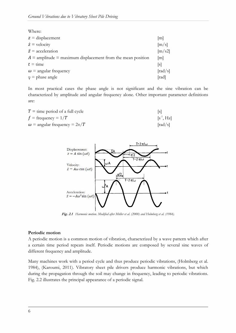
Harmonic motion The most basic type of vibration is the harmonic movement, which can be described by simple sine functions, see Eq. (2.1)-(2.3) below. The displacement is a function of time . These expressions show the relation between displacement, velocity and acceleration of the harmonic vibration, where velocity is the first derivative and acceleration the second derivative of the displacement function, see Fig. 2.1, (Holmberg et al., 1984), (Nordal, 2009).
Displacement: sin (2.1)
Velocity: cos (2.2)
Acceleration: sin (2.3)
Ground Vibrations due to Vibratory Sheet Pile Driving
6
Where: = displacement [m] = velocity [m/s] = acceleration [m/s2] = amplitude = maximum displacement from the mean position [m] = time [s] = angular frequency [rad/s]
φ = phase angle [rad] In most practical cases the phase angle is not significant and the sine vibration can be characterized by amplitude and angular frequency alone. Other important parameter definitions are:
= time period of a full cycle [s] = frequency = 1/ [s-1, Hz] = angular frequency = 2π/ [rad/s]
Fig. 2.1 Harmonic motion. Modified after Möller et al. (2000) and Holmberg et al. (1984).
Periodic motion A periodic motion is a common motion of vibration, characterized by a wave pattern which after a certain time period repeats itself. Periodic motions are composed by several sine waves of different frequency and amplitude.
Many machines work with a period cycle and thus produce periodic vibrations, (Holmberg et al. 1984), (Karoumi, 2011). Vibratory sheet pile drivers produce harmonic vibrations, but which during the propagation through the soil may change in frequency, leading to periodic vibrations. Fig. 2.2 illustrates the principal appearance of a periodic signal.

Literature study
7
Fig. 2.2 Periodic motion.
Transient motion Transient motion can be approximated as an, in time, declining sine vibration, see Fig. 2.3. The movement is initiated with a high intensity which rather quickly fades out, (Möller et al. 2000). Impact driving of piles and sheet piles is an example of an event generating transient vibrations, (Holmberg et al., 1984).
Fig. 2.3 Transient motion.
Random motion Random vibrations are characterized by wave pattern that never repeats themselves, see Fig. 2.4, (Nordal, 2009). Random vibrations often originate from several cooperating sources. Noise vibration and traffic induced vibration are examples of random motions, (Holmberg et al., 1984).
Fig. 2.4 Random motion.

Ground Vibrations due to Vibratory Sheet Pile Driving
8
2.2.2 Vibration analysis When analyzing documented vibration signals, some knowledge about different approaches and tools is needed. Vibrations signals are characterized by several parameters and can be presented in different ways. The following sections will describe the difference between the two most common representations; time domain and frequency domain, as well as the method of converting the signals between the two.
Presentation of vibrations Vibration signals can be presented in time domain or in frequency domain. Previous Fig. 2.1 - Fig. 2.4 show vibrations in the time domain, where particle displacement, velocity or acceleration is expressed as a function of time. The frequency domain shows the dominating frequencies of the vibration. In Fig. 2.5, the difference between these two representations can be seen, as well as the characteristic appearance of each motion of vibration. The frequency domain graphs are also called frequency spectra.
Periodic vibrations containing several frequencies might cause a single mode of vibration to be non-detectable in the time domain. Converting the signal into frequency domain will however divide the vibrations into several sine vibrations and present all frequencies as peaks in the spectrum, see Fig. 2.6. The appearance of the spectrum signals will be influenced by the characteristics of the dynamic system, such as damping and stiffness. For example, a higher damping ratio will lead to a wider peak in the spectrum while a signal with low damping ratio becomes a narrower peak, (Karoumi, 2011).
Fig. 2.6 Time versus spectrum, (Karoumi, 2011).
Fig. 2.5 Characteristics of vibrations. Modified after Möller et al. (2000).

Literature study
9
Fourier Transform Transformation between the time domain and the frequency domain can be performed by using the Fourier Transform. Fourier Transform is an integration method following Eq. (2.4).
(2.4)
Where:
= frequency = time
= frequency domain representation of the signal x = time domain representation of the signal x √ 1
A measured vibration signal presented in time domain consists of a certain number of samples for which the amplitude is measured, e.g. one hundred measurements every second. With a discrete number of samples, a way of converting time dependent signals into a frequency spectrum is by a numerical integration called the Discrete Fourier Transform (DFT), which is an approximation of a true Fourier Transform shown above. A fast way of calculating DFT is an algorithm called Fast Fourier Transform (FFT), which is used in many signal analysis softwares. The transformation is illustrated in Fig. 2.7, (Agilent Technologies, 2000), (Karoumi, 2011).
Fig. 2.7 Fast Fourier Transform, (Agilent Technologies, 2000).

Ground Vibrations due to Vibratory Sheet Pile Driving
10
2.3 Soil dynamics Following sections describe some fundamentals of soil dynamics. Dynamic loading is characterized by short duration, but repeated loading. The soil behavior in dynamic situations will differ from that under static circumstances. Soil dynamics include understanding of soil properties influencing the dynamic behavior, how the waves propagate through the material and also the mechanisms behind attenuation of the wave motions as the distance to the source increases.
2.3.1 Dynamic parameters What characterize dynamic systems are mainly the stiffness and damping properties. Considering soil dynamics, the main soil parameters influencing these dynamic properties are the wave propagation velocity, Poisson’s ratio and the material damping, (Hintze et al., 1997). The shear modulus, which is a stiffness parameter, is affected by dynamic loading and will differ from static situations, (Holeyman, 2002).
Wave propagation velocity
A distinction is made between the wave propagation velocity, , and the particle velocity, . As previously mentioned, the particle velocity describes the particles movement around a state of equilibrium. The wave propagation velocity is a measure of how fast the wave travels away from the source and can be expressed in terms of frequency and wave length, Eq. (2.5).
∙ (2.5)Where: = wave propagation velocity [m/s] = frequency [Hz] = wave length [m]
Wave propagation velocity is dependent of the elastic properties of the soil material and is in general lower in soft soils than in stiff soils. The propagation velocity increases with a higher Poisson’s ratio and a lower void ratio of the soil, (Hintze et al., 1997). Different types of waves and their corresponding wave velocities are described in section 2.3.2.
Poisson’s ratio As a material is stretched in one direction, it tends to contract in the other direction. This phenomenon is called the Poisson effect. Poisson’s ratio is usually denoted as and is the ratio between the strain, , in transverse and axial direction of the applied force, see Eq. (2.6), (Santamarina et al., 2001).
(2.6)
Where: = Poisson’s ratio [ - ]
= strain in transversal direction (negative for tension, positive for compression) [%] = strain in axial direction (positive for tension, negative for compression) [%]

Literature study
11
The Poisson ratio of the soil influence the wave propagation velocity but also the vibration amplitude. Both parameters increase with a higher value of Poisson ratio. Tab. 2.1 presents common values of Poisson’s ratio for different soil types, suggested by Hintze et al. (1997).
Tab. 2.1 Poisson's ratio for different soil types. After Hintze et al. (1997).
Soil type Poisson’s ratio
Clay 0,45 – 0,5
Dry sand 0,25 – 0,35
Moraine 0,4 – 0,5
Rock 0,4 – 0,5
Material damping Material damping describes the absorption of wave energy due to friction within the material, causing the wave to attenuate with distance, (Holmberg et al., 1984). Attenuation of wave propagation is further described in section 2.3.3.
The material damping is dependent of the wave propagation velocity. Since soft soils have lower propagation velocities than stiff soils, motions with the same frequency will have shorter wave lengths in softer soils. This means that for a certain distance, the waves in soft soils will experience more cycles of motion and experience more material damping than waves traveling through stiffer soils with higher propagation velocities. At a certain distances from the source of vibration, the particle velocity will thus be smaller in softer soils, (Dowding, 1996).
Shear modulus The shear modulus is a measure of the soil stiffness when shearing, which according to Möller et al. (2000) is mainly dependent of the effective stress and void ratio of the soil. Möller et al. (2000) propose an empirical formulation for determining the shear modulus of frictional soils according to Eq. (2.7).
∙ ∙
1∙ (2.7)
Where:
= shear modulus [Pa] , , = material constants according to Tab. 2.2 [ - ]
= void ratio [ - ] = average effective stress [Pa]

Ground Vibrations due to Vibratory Sheet Pile Driving
12
Tab. 2.2 Material constants for Eq. (2.7) .
Soil type
Sand 16600 2,17 0,4
Coarse material 7230 2,97 0,38
Crushed rock 13000 2,17 0,55
Round-grained gravel 8400 2,17 0,6
The shear modulus can according to elastic theory also be expressed in terms of the elastic modulus and Poisson ratio, according to Eq. (2.8), ( Santamarina et al., 2001).
2 1
(2.8)
Where:
= shear modulus [Pa] = shear stress [Pa] = shear strain [ - ] = elastic modulus [Pa] = Poisson ratio [ - ]
The shear modulus is highly strain dependent. Eq. (2.8) is only valid when the soil behaves elastically, which is for strains smaller than 10-3. The shear modulus begins to decrease with strains larger than 10-5, while the material damping increases. At strains larger than 10-2 however, both shear modulus and material damping will decrease because of the cyclic loading, (Möller et al., 2000). With every load cycle, the soil structure will deteriorate, pore water pressure will increase and the shear modulus will decrease. This degradation of the soil depends mainly on the number of cycles, the magnitude of the cyclic strain and the characteristics of the soil material, (Holeyman, 2002).
2.3.2 Wave propagation In a vibration motion, the particles move around a state of equilibrium. However, there are different motions where this is fulfilled, which will affect the propagation velocity. Different types of wave motions and mechanisms appearing in soil are presented in this section:
Waves in full space – body waves
Waves in half space – surface waves
Waves in layered material – reflection, refraction and interference
Resonance
One basic assumption which is usually made in the theory of soil dynamics is the description of the soil as a linear elastic material. In the real world the soil material is better described as an elasto-plastic material, but which at very small deformations behaves completely elastic (Möller et al., 2000). When the soil is subjected to shear strains smaller than 10-3 %, the soil is completely

Literature study
13
elastic. With a strain level in the range of 10-3 to 10-1, the soil shows an elasto-plastic behavior with some permanent deformations. When the soil is subjected to larger strains than 10-1 the soil is in a failure condition with plastic deformations. During vibratory driving, the soil in the immediate vicinity of the sheet pile is actually at failure, but the strain attenuates quickly into the elasto-plastic and later elastic zone, (Massarsch, 2002). According to Bodare (1996), the linear-elastic model has proven to be a good approximation to real field behavior, why it is applied when describing the wave propagation in the sections below.
Waves in full space A three dimensional material such as soil can be approximated as a full space, where the material is linear-elastic and infinite in all directions. In full space there are two types of wave motion. One is associated with a volume change, while the other is associated with a change of shape. The description of these wave motions are based on Holmberg et al. (1984), Bodare (1996), Hintze et al. (1997) and Day (2002).
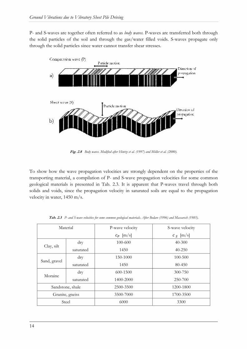
The first of the two is a compressional wave, where the particle motion is longitudinal, i.e. parallel to the direction of the wave propagation, see Fig. 2.8a. The compression wave is also called the primary wave, or shorter P-wave, since it has the highest velocity, see Tab. 2.3. The wave propagation velocity is a material constant and can for a P-wave be expressed according to following Eq. (2.9).
∙1
1 2 1 (2.9)
Where:
= compression wave velocity [m/s] = constrained modulus [Pa]
= total density [kg/m3] = modulus of elasticity [Pa] = Poisson’s ratio [ - ]
The other type of wave is a transversal shear wave, where the particle motion is perpendicular to the direction of the wave propagation, see Fig. 2.8b. The shear wave is slower than the compression wave, see Tab. 2.3, why it is called the secondary wave, or S-wave. The wave propagation velocity of the S-wave, , can be expressed according to Eq. (2.10), with the same parameters as above and is the shear modulus in Pa.
∙1
2 1 (2.10)
Ground Vibrations due to Vibratory Sheet Pile Driving
14
P- and S-waves are together often referred to as body waves. P-waves are transferred both through the solid particles of the soil and through the gas/water filled voids. S-waves propagate only through the solid particles since water cannot transfer shear stresses.
Fig. 2.8 Body waves. Modified after Hintze et al. (1997) and Möller et al. (2000).
To show how the wave propagation velocities are strongly dependent on the properties of the transporting material, a compilation of P- and S-wave propagation velocities for some common geological materials is presented in Tab. 2.3. It is apparent that P-waves travel through both solids and voids, since the propagation velocity in saturated soils are equal to the propagation velocity in water, 1450 m/s.
Tab. 2.3 P- and S-wave velocities for some common geological materials. After Bodare (1996) and Massarsch (1985).
Material P-wave velocity S-wave velocity
[m/s] [m/s]
Clay, silt dry 100-600 40-300
saturated 1450 40-250
Sand, gravel dry 150-1000 100-500
saturated 1450 80-450
Moraine dry 600-1500 300-750
saturated 1400-2000 250-700
Sandstone, shale 2500-3500 1200-1800
Granite, gneiss 3500-7000 1700-3500
Steel 6000 3300
Literature study
15
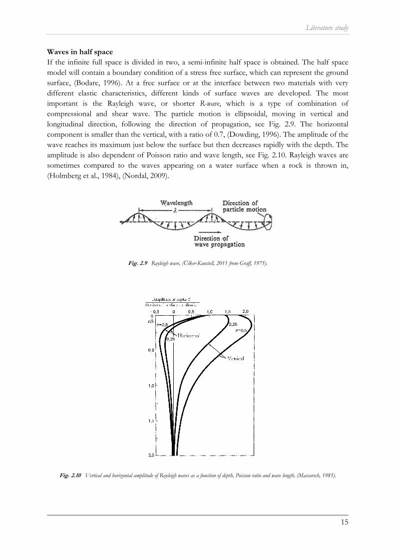
Waves in half space If the infinite full space is divided in two, a semi-infinite half space is obtained. The half space model will contain a boundary condition of a stress free surface, which can represent the ground surface, (Bodare, 1996). At a free surface or at the interface between two materials with very different elastic characteristics, different kinds of surface waves are developed. The most important is the Rayleigh wave, or shorter R-wave, which is a type of combination of compressional and shear wave. The particle motion is ellipsoidal, moving in vertical and longitudinal direction, following the direction of propagation, see Fig. 2.9. The horizontal component is smaller than the vertical, with a ratio of 0.7, (Dowding, 1996). The amplitude of the wave reaches its maximum just below the surface but then decreases rapidly with the depth. The amplitude is also dependent of Poisson ratio and wave length, see Fig. 2.10. Rayleigh waves are sometimes compared to the waves appearing on a water surface when a rock is thrown in, (Holmberg et al., 1984), (Nordal, 2009).
Fig. 2.9 Rayleigh wave, (Ülker-Kaustell, 2011 from Graff, 1975).
Fig. 2.10 Vertical and horizontal amplitude of Rayleigh waves as a function of depth, Poisson ratio and wave length, (Massarsch, 1985).

Ground Vibrations due to Vibratory Sheet Pile Driving
16
The R-wave attenuates slower than P- and S-waves, why it is usually the only detectable wave at long distances from the source of vibration. Compared to the body waves, the R-wave is slightly slower than the S-wave, (Holmberg et al., 1984). Because of the low frequency, long duration and large amplitude of the Rayleigh wave, it is often the most destructive wave type and thus of most practical interest for engineers, (Svinkin, 2008).
Since the R-wave is a sort of reflection of P- and S-waves, the wave propagates through both the solids and the pore water in the soil, (Hintze et al., 1997). According to Bodare (1996) the wave propagation velocity, , can be approximated with following expression.
0.87 1.12
1∙ (2.11)
With, in geotechnical engineering, commonly used values of the Poisson ratio the expression can be further approximated to Eq. (2.12), where it is apparent that the Rayleigh waves and shear waves have quite similar propagation velocity.
0.93 (2.12)
Another type of surface wave is called Love wave, or shorter L-wave, which only appears in layered material. L-waves develop when shear waves in a layer with a lower propagation velocity,
, hits the interface to a layer with a higher propagation velocity, . If the angle of approach is larger than / , a complete reflection of the wave back into the layer occurs. All of the wave energy remains in the layer which allows the wave to propagate long distances within the layer, (Bodare, 1996).
Waves in layered material Soil profiles are in reality usually layered, with varying material properties along the depth. Since the wave propagation is dependent on the elastic properties of the soil, it will be affected if these properties change along the wave path, (Bodare, 1996).
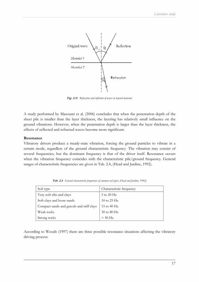
When a wave hits an interface of a new material with different properties, the angle and velocity of the wave will change. This phenomenon is referred to as refraction. An interface between two materials may also cause the wave to reflect back into the original material. The velocity of a reflected or refracted wave can be greater than that of the incident wave. The amplitude and direction of the resultant waves depend on the angle of incident at the boundary and the ratio of densities of the materials, see Fig. 2.11. Surface waves are results of reflection of body waves. Rayleigh waves are generated at the ground surface, while Love waves are generated at the interfaces of layers below the surface, (Head and Jardine, 1992).
If several waves exist in the same area they will be added to one another, causing a phenomenon called interference. Two waves in phase will cause an amplification of the wave, while two waves out of phase will weaken the wave, (Möller et al., 2000).
Literature study
17
Fig. 2.11 Refraction and reflection of waves in layered material.
A study performed by Masoumi et al. (2006) concludes that when the penetration depth of the sheet pile is smaller than the layer thickness, the layering has relatively small influence on the ground vibrations. However, when the penetration depth is larger than the layer thickness, the effects of reflected and refracted waves become more significant.
Resonance Vibratory drivers produce a steady-state vibration, forcing the ground particles to vibrate in a certain mode, regardless of the ground characteristic frequency. The vibration may consist of several frequencies, but the dominant frequency is that of the driver itself. Resonance occurs when the vibration frequency coincides with the characteristic pile/ground frequency. General ranges of characteristic frequencies are given in Tab. 2.4, (Head and Jardine, 1992).
Tab. 2.4 General characteristic frequencies of common soil types, (Head and Jardine, 1992).
Soil type Characteristic frequency
Very soft silts and clays 5 to 20 Hz
Soft clays and loose sands 10 to 25 Hz
Compact sands and gravels and stiff clays 15 to 40 Hz
Weak rocks 30 to 80 Hz
Strong rocks > 50 Hz
According to Woods (1997) there are three possible resonance situations affecting the vibratory driving process:
Ground Vibrations due to Vibratory Sheet Pile Driving
18
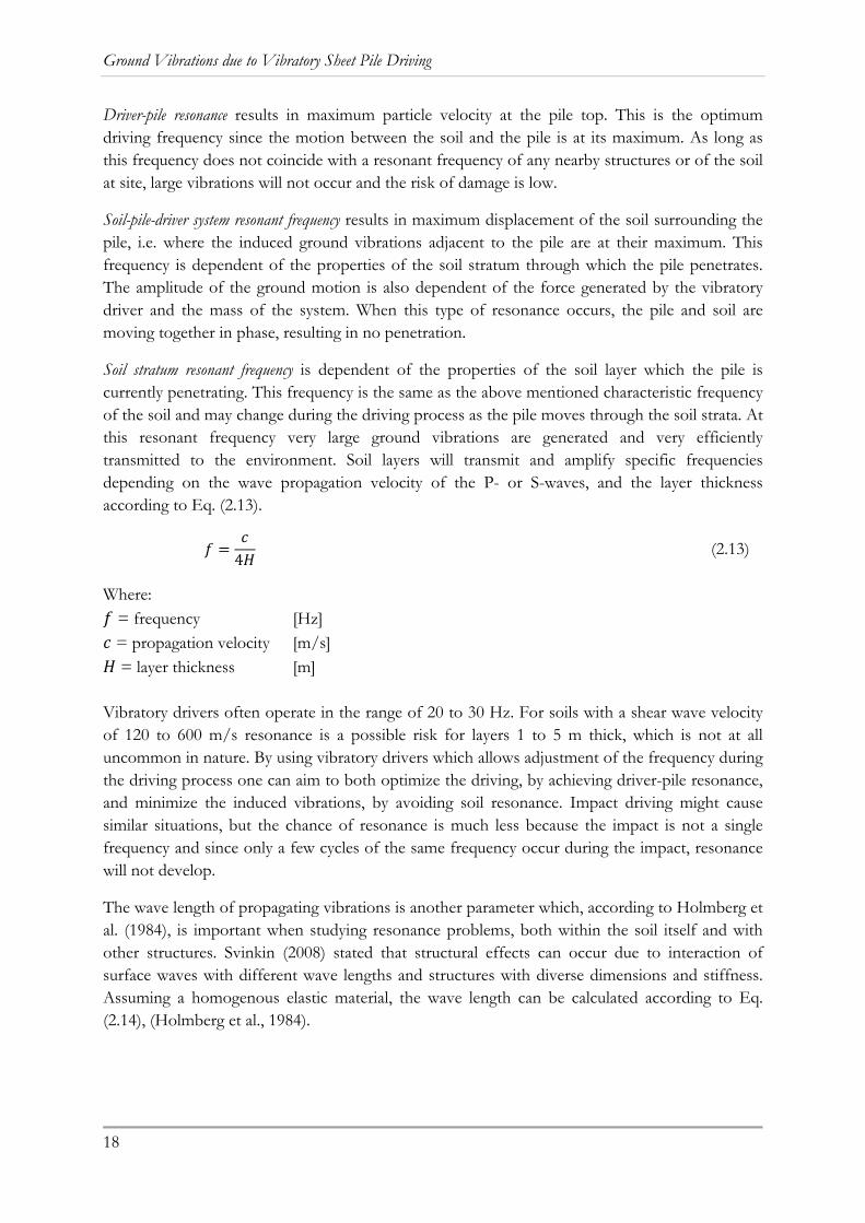
Driver-pile resonance results in maximum particle velocity at the pile top. This is the optimum driving frequency since the motion between the soil and the pile is at its maximum. As long as this frequency does not coincide with a resonant frequency of any nearby structures or of the soil at site, large vibrations will not occur and the risk of damage is low.
Soil-pile-driver system resonant frequency results in maximum displacement of the soil surrounding the pile, i.e. where the induced ground vibrations adjacent to the pile are at their maximum. This frequency is dependent of the properties of the soil stratum through which the pile penetrates. The amplitude of the ground motion is also dependent of the force generated by the vibratory driver and the mass of the system. When this type of resonance occurs, the pile and soil are moving together in phase, resulting in no penetration.
Soil stratum resonant frequency is dependent of the properties of the soil layer which the pile is currently penetrating. This frequency is the same as the above mentioned characteristic frequency of the soil and may change during the driving process as the pile moves through the soil strata. At this resonant frequency very large ground vibrations are generated and very efficiently transmitted to the environment. Soil layers will transmit and amplify specific frequencies depending on the wave propagation velocity of the P- or S-waves, and the layer thickness according to Eq. (2.13).
4
(2.13)
Where:
= frequency [Hz] = propagation velocity [m/s] = layer thickness [m]
Vibratory drivers often operate in the range of 20 to 30 Hz. For soils with a shear wave velocity of 120 to 600 m/s resonance is a possible risk for layers 1 to 5 m thick, which is not at all uncommon in nature. By using vibratory drivers which allows adjustment of the frequency during the driving process one can aim to both optimize the driving, by achieving driver-pile resonance, and minimize the induced vibrations, by avoiding soil resonance. Impact driving might cause similar situations, but the chance of resonance is much less because the impact is not a single frequency and since only a few cycles of the same frequency occur during the impact, resonance will not develop.
The wave length of propagating vibrations is another parameter which, according to Holmberg et al. (1984), is important when studying resonance problems, both within the soil itself and with other structures. Svinkin (2008) stated that structural effects can occur due to interaction of surface waves with different wave lengths and structures with diverse dimensions and stiffness. Assuming a homogenous elastic material, the wave length can be calculated according to Eq. (2.14), (Holmberg et al., 1984).

Literature study
19
(2.14)
Where:
= wave length [m] = wave propagation velocity [m/s] = frequency [s-1]
The wave length is also important to consider when taking vibration mitigation measures. Woods (1997) states that based on experiments and numerical models it has been shown that an effective wave barrier must be at least two-thirds of a wave length deep and at least one wave length long to reduce the vibration amplitude with about 88 percent. With wave lengths commonly varying from 3 to 150 m, wave barriers must often be very long and deep.
2.3.3 Attenuation The intensity of vibrations decrease as the wave propagates away from the source. Attenuation of the vibration is dependent of mainly two damping factors; the geometry of the propagation and the material in which the waves propagate, (Holmberg et al., 1984), (Hintze et al., 1997).
Geometrical damping Geometrical damping is the major mechanism behind the attenuation of vibrations. As the vibration propagates, the same amount of energy is distributed over an increasingly larger volume or surface causing a decrease of amplitude. The geometrical damping varies with different wave types and is proportional to following ratios, where is the distance from the source of vibration, (Holmberg et al., 1984), (Nordal, 2009).
Body waves:
Body waves along the surface:
Rayleigh waves: √
From these relations it is apparent that surface waves, like Rayleigh waves, attenuate slower than the body waves. That is why surface waves often are most significant in practical cases, (Hintze et al., 1997).
Material damping Material damping is an internal damping where, with each cycle of oscillation, some energy is absorbed into the material as internal frictional losses as the particles move against each other. Energy from the wave is transformed into heat energy along the grain boundaries, (Holmberg et al., 1984), (Hintze et al., 1997).
Material damping is often described by a damping factor α, also called absorption coefficient, which is generally lower for hard materials and higher for soft materials. The damping factor is highly frequency dependent in a linear manner, making it easy to compute the damping factor for

Ground Vibrations due to Vibratory Sheet Pile Driving
20
one frequency if it is known for another frequency, according to Eq. (2.15). Lower frequencies do not receive as much damping as higher frequencies, enabling waves of lower frequency to propagate further. Tab. 2.5 presents damping factors for different soil types, calculated for a frequency of 30 Hz, (Woods, 1997).
(2.15)
Where:
= damping factor at frequency = damping factor at frequency
Tab. 2.5 Damping factors of different soil types. After Woods (1997).
Damping factor α [m-1] at 30 Hz Material description
0.06 – 0.195 Weak or soft soils – dry peat and muck, mud, loose beach sand, dune sand, recently plowed ground, organic soil. (shovel penetrates easily)
0.0195 – 0.06 Competent soils – sand, sandy clays, silty clays, gravel, silt, weathered rock. (can dig with shovel)
0.00195 – 0.0195 Hard soils – dense compacted sand, dry consolidated clay, consolidated glacial till, some exposed rock. (cannot dig with shovel)
< 0.00195 Hard, competent rock – bedrock, freshly exposed hard rock. (difficult to break with hammer)
Attenuation relationship Considering both the material and geometrical damping, the relation presented in Eq. (2.16) can be used to describe the total damping effect on the wave amplitude, (Holmberg et al., 1984), (Woods, 1997). The origin of this equation dates back to 1912 when Golitsin derived it specifically for Rayleigh waves generated by earthquakes, but it has later been adjusted for application on different kinds of waves, (Svinkin, 2008).
(2.16)
Where:
= amplitude at distance from the source [m] = amplitude at distance from the source [m]
= 1 for body waves 2 for body waves along the surface ½ for Rayleigh waves
= absorption coefficient describing material damping [m-1]
Literature study
21
2.4 Vibratory driving of sheet piles Vibratory driving was developed in Russia in the early 1930’s and has since then become an increasingly used technique in many countries. Even though the development of the machinery is extensive, there are still hesitations among engineers to the use of this method. There is still a lack of knowledge, experience and research considering the mechanisms behind vibratory driving, (Massarsch, 2000), (Viking, 2004).
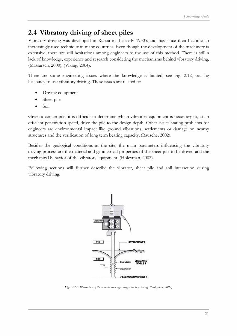
There are some engineering issues where the knowledge is limited, see Fig. 2.12, causing hesitancy to use vibratory driving. These issues are related to:
Driving equipment
Sheet pile
Soil
Given a certain pile, it is difficult to determine which vibratory equipment is necessary to, at an efficient penetration speed, drive the pile to the design depth. Other issues stating problems for engineers are environmental impact like ground vibrations, settlements or damage on nearby structures and the verification of long term bearing capacity, (Rausche, 2002).
Besides the geological conditions at the site, the main parameters influencing the vibratory driving process are the material and geometrical properties of the sheet pile to be driven and the mechanical behavior of the vibratory equipment, (Holeyman, 2002).
Following sections will further describe the vibrator, sheet pile and soil interaction during vibratory driving.
Fig. 2.12 Illustration of the uncertainties regarding vibratory driving, (Holeyman, 2002).

Ground Vibrations due to Vibratory Sheet Pile Driving
22
2.4.1 Driving equipment Vibratory machinery has been greatly improved over the last decades. Initial improvements were focused on increasing the speed of the technique, while more recent improvements attempt to reduce environmental impact. The first vibrators were heavy, electrically driven machines. Modern day vibrators are almost exclusively hydraulically driven, which due to a smaller motor are smaller and lighter compared to the electrical machines. Hydraulic systems also allow adjustment of both frequency and eccentricity. The main components of the driving system are a power source, power transmission, vibrator, sheet pile and some sort of carrier, (Massarsch, 2000), (Holeyman, 2002), (Viking, 2004).
Two types of systems are available today, either the free hanging or the leader mounted system. Free hanging systems cost less and have greater reaching capabilities, while it is lacking in control over the positioning of the sheet pile and in changing the static surcharge force during installation. Leader mounted systems are more expensive but works with higher precision considering positioning, displacement amplitude and driving/extracting forces. Where the bearing capacity of the underlying soil is low, the free hanging system might be favorable since they are lighter than the leader mounted systems, (Viking, 2004).
Vibrator unit The vibratory unit is the part of the equipment which generates the sinusoidal motion of the sheet pile. The main parts of a vibrator are:
Bias mass
Elastomer pads (or springs)
Eccentric masses
Clamp
Bias mass, or suppressor housing, is the non-vibrating part of the vibrator. The bias mass is a static mass which both increases the driveability and serves as a connection to the crane line or leader mast. Electrical and hydraulic cables are also connected to the bias mass.
Springs or elastomer pads connects and isolates the non-vibrating parts from the vibrating parts.
Eccentric masses constitute the vibrating part of the unit. Several eccentric masses together with a gearbox and the hydraulic motor form the exciter block. The vertical oscillating force is generated by counter-rotating the eccentric masses.
The clamp forms a rigid connection between the sheet pile and the vibro-unit, transferring the generated force to the profile.
Fig. 2.13 shows the principal components of the vibrator alone while Fig. 2.14 illustrates an example of a free hanging system with more parts included. In a leader mounted system, the eccentric masses are usually placed vertically, for a slimmer design, (Massarsch, 2000), (Viking, 2004).

Literature study
23
The driving frequency of the vibrator has a great impact on the generated driving force. The vibratory systems, free hanging or leader mounted, can be categorized based on the driving frequency, , and variability of the eccentric moment, . Tab. 2.6 is a compilation of vibrator types classified by driving frequency and eccentric moment.
Tab. 2.6 Vibrator types, (Viking, 2002 and 2004).
Type of vibrator Range of [Hz] Range of [kgm]
Standard frequency 21 - 30 > 230
High frequency 30 - 42 6 -45
Variable eccentricity 30 - 40 10 - 54
Excavator mounted 30 - 50 1 - 13
Resonant driver > 100 50
As described in section (2.3.2) there is an issue concerning resonance within the soil. When the driving frequency and the characteristic frequency of the soil coincide, resonance effects occur which amplifies the ground vibrations. Since the characteristic frequencies of soils often are lower than the driving frequency, this usually occurs during startup of the machine, before it reaches the full driving frequency, and in a similar way when shutting down. When both the driving frequency and eccentricity can be adjusted continuously during the driving process, i.e. when the vibratory motion is not initiated until the driving frequency is reached, this resonance problem can be avoided and the induced ground vibrations are in turn reduced. The optimized situation would be to pass the critical resonant frequencies of the soil and pile without any force applied
Fig. 2.13 Vibrator components. 1) Eccentric masses. 2) Clamp. 3)Springs, (Massarsch,2000).
Fig. 2.14 Principles of the vibratory driving machinery. Modified after Massarsch (2000).

Ground Vibrations due to Vibratory Sheet Pile Driving
24
and then as the driver-pile resonant frequency is reached increase the force level to efficiently drive the sheet pile. The vibrators where this can be controlled are usually called “variable eccentricity”, “variable amplitude” or “resonant free” vibrators, (Woods, 1997), (Viking, 2002).
Vibratory driving parameters This section will present parameters of importance when describing the mechanical actions of the vibratory system. From Massarsch (2000) and Viking (2002 and 2004), following theoretical parameters can be distinguished as the most important:
Static surcharge force
Eccentric moment
Dynamic centrifugal force
Displacement amplitude
The generated driving force consists of one stationary and one dynamic part, where the stationary part is denoted as static surcharge force. The dynamic part is the vertical component of a sinusoidal centrifugal force generated when the eccentric masses, arranged in pairs, are rotated at the same speed but in opposite direction.
(2.17) Where:
= driving force [N] = static surcharge force [N] = centrifugal force [N]
The static surcharge force is in a free hanging system equal to the dead weight of the bias mass minus the force in the suspension to the crane, according to Eq. (2.18).
(2.18) Where:
= gravity [m/s2]
0 = bias mass [kg] = suspension force [N]
In leader mounted system, the suspension force is replaced with the hydraulically applied pressure, according to Eq. (2.19).
(2.19)

Literature study
25
Where:
0 = hydraulic oil pressure [N/m2] = area of hydraulic cylinder [m2]
The dynamic centrifugal force depends on the static moment, or eccentric moment, which is the product of the eccentric masses and their individual distance from their centre of gravity to the centre of the motor shaft, see Eq. (2.20) and Fig. 2.15.
(2.20)
Where:
= eccentric moment [kgm] = one eccentric mass [kg]
= eccentric radius [m]
The centrifugal force is dependent of the driving frequency of the vibrator and the eccentric moment, according to following Eq. (2.21).
2 260
(2.21)
Where:
= driving frequency [Hz] = rotations per minute [rpm] = angular velocity [rad/s]
The vertical component of the centrifugal force is given by Eq. (2.22). According to Fig. 2.16 it is apparent that the horizontal components will be cancelled out.
sin sin (2.22) Where:
= rotation angle of eccentric mass [ °]
Fig. 2.15 Eccentric mass and radius. (Viking, 2002)
Fig. 2.16 Centrifugal force. (Viking, 2002)

Ground Vibrations due to Vibratory Sheet Pile Driving
26
The displacement amplitude is often described by the double amplitude, i.e. the peak to peak displacement. The double amplitude is usually denoted with uppercase letter, , while the single amplitude is denoted by lower case, . The double displacement amplitude, Eq. (2.23), is dependent of the eccentric moment and the “dynamic mass”, which is the mass of the vibrating parts.
2 2 (2.23)
Where:
= double amplitude [m]
= single amplitude [m] = eccentric moment [kgm]
= dynamic mass [kg]
A value of the maximum displacement amplitude is usually given in the specifications of vibrators. However, this value is always higher than the real double amplitude because the mass of the sheet pile is not included. Soil and interlock resistance is also a reason for a lower actual displacement amplitude, (Viking, 2002), (Van Baars, 2004).
2.4.2 Sheet piles Sheet piles are steel profiles installed as either temporary or permanent retaining structures with primary purpose to withstand lateral earth pressure during excavations. Individual sheet piles are connected to each other by an interlock, forming a solid wall. Some sheet pile walls are waterproof, ensuring that the groundwater level behind the wall is not lowered. To restrict movement of the sheet pile wall, it can be stabilized by e.g. struts or tie-back anchors, (Day, 2002).
Holeyman (2002) characterize the profiles by following parameters:
: profile section [m2]
: profile length [m]
: profile parameter [m] : Young’s modulus [MPa]
: density [kg/m3]
The longitudinal wave velocity in the profile can be calculated by Eq. (2.24).
/ (2.24) Besides the sectional properties of the profile, two other parameters will affect both the driveability of the sheet piles as well as the induced ground vibrations. As the sheet piles are driven together a frictional force, also referred to as clutch friction, , is generated in the interlock. The friction is caused mainly by soil particles in the interlocks but also by friction

Literature study
27
between the steel. Experience has shown that the influence of the clutch friction may cause a three to five times increase of the vertically induced ground vibrations. The magnitude of the clutch friction is dependent of the condition of the interlocks. Using new sheet piles and driving the piles with an accurate angle towards each other will significantly reduce the interlock friction and thus the induced ground vibrations, (Deckner et al., 2010).
The other parameter which is important to acknowledge is the fact that the driving force is applied eccentrically to the profiles, due to the way of clamping the profiles, see Fig. 2.17. The clamping devices are generally designed to clamp the sheet piles by the web, which is not the neutral layer of the profile. The eccentric position of the driving force gives rise to an unfavorable bending moment and causes a lateral movement of the profile, . The lateral induced vibrations may be two to three times larger than the vertically induced. A different clamping configuration where the driving force is applied in the neutral layer of the sheet piles would reduce the lateral movement and thus the environmental impact, (Viking, 2004), (Deckner et al., 2010).
Fig. 2.17 Lateral movement. Modified after Viking et al. (2000).
Ground Vibrations due to Vibratory Sheet Pile Driving
28
2.4.3 Impedance Massarsch and Fellenius (2008) highlights a parameter called impedance, as the most important factor influencing the transfer of wave energy between the sheet pile and the surrounding soil. The amount of transferred energy is connected to the relation between the pile and soil impedance.
The pile impedance, , is dependent of the pile density, the wave propagation velocity in the pile and the cross section area of the pile. The pile impedance can also be expressed as a function of the modulus of elasticity, see Eq. (2.25), (Massarsch, 2000).
∙ ∙∙
(2.25)
Where:
= pile impedance [Ns/m]
= pile material density [kg/m3] = wave propagation velocity in the pile [m/s]
= cross section area of the pile [m2]
= modulus of elasticity [Pa] With the sheet pile impedance and oscillation velocity of the particles (not the same as propagation velocity ) known, the dynamic force transferred to the sheet pile can be calculated according to Eq. (2.26). It is evident from this relation that a decrease of pile impedance will cause an increase of vibration magnitude. The sheet pile impedance restricts the maximal force propagated through the profile toward the profile toe, (Massarsch, 2000).
∙ (2.26) Where:
= dynamic force [N] = sheet pile oscillation speed [m/s]
During installation of the sheet pile, dynamic soil resistance will develop along the profile. The soil impedance will influence this resistance, (Massarsch and Fellenius, 2008). Considering the soil, a difference is made between the soil impedance, , and the specific soil impedance, , where the impedance is the product of the specific impedance and the contact area between pile and soil. Eq. (2.27) shows the expression of the specific soil impedance, (Bodare, 1996).
∙ ∙ (2.27)
Where: = specific soil impedance [Ns/m3] = shear modulus [Pa] = soil density [kg/m3] = shear wave velocity at sheet pile-soil interface [m/s]

Literature study
29
2.4.4 Soil resistance The wave energy produced by the vibratory driver is transferred from the sheet pile to the surrounding soil through the dynamic soil resistance. This resistance is the sum of developed resistance along the shaft, , at the toe, , and as the sheet pile is driven into the interlock, , (Viking, 2004). Vibratory driving of sheet piles is most effective in loose non-cohesive soils,
due to the favorable reduction of the dynamic soil resistance in this kind of soil. Cohesive or very dense non-cohesive soils do not show the same behavior, (Viking, 2002). In cohesive soils, both
and increase with the driving frequency. In order to overcome the soil resistance, a low driving frequency as well as a large displacement amplitude is required, (Massarsch, 2000).
Compared to impact driving where the initial static resistance of the soil needs to be overcome with every blow, the sheet pile is constantly in the driving state during vibratory driving, where the initial static resistance is already overcome. This is the main reason for the favorable reduction of the shaft resistance. The toe however looses contact with the underlying soil with each vibration cycle and will cause a small displacement of soil volume with every downward motion, (Deckner et al., 2010).
The dynamic resistance is varying along with the up- and downward motion of the sheet pile being driven, see Figure 2.18. The shaft resistance varies between positive and negative and the toe resistance varies between zero and maximum, where the maximum is reached at the lower end of the vibration motion of the sheet pile, (Viking, 2000).
Figure 2.18 Illustration of the relationship between: a) Penetrative motion of the sheet pile b) Shaft resistance c) Toe resistance. Modified after Viking (2000).
Vibratory driving of sheet piles subjects the soil to cyclic loading with large strain cycles. When subjected to cyclic loading, the soil resistance will degrade due to fatigue of the soil skeleton in cohesive soils and effective stress reduction in non-cohesive soils. With each cycle, the soil structure continuously deteriorates, the pore water pressure increases and the shear modulus decreases. Holeyman (2002) refers to this process as cyclic stiffness degradation.
Ground Vibrations due to Vibratory Sheet Pile Driving
30
Vibration of saturated, loose sand or silt can result in a phenomenon called liquefaction. The cyclic loading causes an increase of pore water pressure, which in turn reduces the contact pressure between the soil particles. This loss of strength in the soil can in the extreme case give an effective stress that is reduced close to zero causing a liquid-like behavior of the soil. The intensity and duration of vibrations and the rate of dissipation of the excess pore water pressure will determine whether liquefaction occurs or not, (Holeyman, 2002).
2.4.5 Wave propagation from the sheet pile Fig. 2.19 illustrates how the wave motion is transferred from the sheet pile to the surrounding soil. Vibrations are generated through the dynamic soil resistance along the shaft and at the toe of the profile. During driving, the sheet pile can be considered to vibrate as a rigid body, i.e. the top of the sheet pile moves at the same time as the toe. The shaft resistance will generate S-waves along the sheet pile surface which due to the rigid body behavior will propagate outwards with a cylindrically shaped wave front. At the toe, an amount of soil volume is displaced with every downward movement, generating body waves propagating in all directions from the toe. These P- and S-waves propagate from the toe with spherical wave fronts. When the P- and S-waves reach the ground surface, part of the wave energy is reflected back into the soil and the other part is converted into generating surface Rayleigh waves, (Attewell and Farmer, 1973).
The generated vibrations will have components in both vertical and horizontal directions, where the horizontal components can be about 30-50 % of the vertical component. The horizontal components increase with the friction angle of the soil and thus larger in frictional soils than in cohesive, (Massarsch, 2000).
Rayleigh waves are not produced at the source, but are still formed at a close distance. The distance is a function of the wave propagation velocities, see Eq. (2.28). Dowding (1996) presents an example for impact driven piles with common parameter values: = 1500 m/s, = 300 m/s and a driving depth of 6 m. According to Eq. (2.28), Rayleigh waves would be produced within 1 to 2 m from the pile.
(2.28)
Where:
= distance between source and origin of Rayleigh waves [m] = Rayleigh wave propagation velocity [m/s] = compression wave propagation velocity [m/s]
= driving depth [m]

Literature study
31
Fig. 2.19 Wave propagtion during vibratory driving. Modified after Attewell and Farmer (1973).
As described in section 2.4.1, the driving force is often applied eccentrically due to clamping beside the neutral layer of the sheet pile, causing the profile to also vibrate laterally during driving. This lateral movement causes not only shear waves to develop along the shaft, but also compressional P-waves, (Viking et al., 2000).
As vibrations propagate away from the source, the characteristics of the vibrations will change from the harmonic motion produced by the vibratory driver. According to Svinkin (2008), the main cause of changes from one observation point to another is the fact that high frequency vibrations attenuate faster with distance from the source. This was also noted by Masoumi et al. (2006) who, during field tests, observed that the frequency content of the ground vibrations change toward lower frequencies as the distance from the pile increases.
The site-specific soil stratification will also affect the behavior of the vibrations, a fact also recognized by Head and Jardine (1992). Stiff soils and rock transmit vibrations more easily than softer soils. Presence of harder layers in the soil profile through which the pile penetrates may thus give rise to high vibration intensities.
Field tests were performed by Whenham et al. (2009) where it was observed that the variation in soil particle velocity was a result of a combination of varying soil resistance, penetration velocity

Ground Vibrations due to Vibratory Sheet Pile Driving
32
and driving frequency. The most obvious factors giving higher vibration magnitudes were however an increase of soil resistance or a decrease of penetration velocity.
As described in section 2.3.3 and visualized in Fig. 2.19, the particle motions have components in three perpendicular directions; vertical, transversal and longitudinal. In field tests it is necessary to measure in all three directions to get a satisfactory representation of the vibrations, due to the nature of the propagating waves. It might however sometimes be practical to combine these into a resulting velocity. This is usually done by using the Peak Particle Velocity, or , which is the vector sum of all components at the same time, see Eq. (2.29).
(2.29)
Whenham et al. (2009) concluded that the horizontal vibrations is not negligible compared to the vertical vibrations. It was also found by studying the frequency spectra that harmonic frequencies are more developed in the horizontal directions. This fact was also recognized by Svinkin (1996), where it was stated that the transversal components have higher frequency content than the longitudinal.

Literature study
33
2.5 Data acquisition To register and present vibration events some type of measurement instrumentation is needed, usually consisting of transducers, recording instrumentation and communication system between the two. Data acquisition systems can range from simple portable readouts to complex automatic systems, (Dunnicliff, 1993). The transducers convert physical motion or pressure to an electrical current. The output signal is transmitted through cables to an amplifying system and later to a tape, digital or paper recorder, (Dowding, 1996).
2.5.1 Measurement transducers Measurements of vibrations are usually performed by measuring amplitude of motion as a function of time. Vibrations can be described by either particle displacement, velocity or acceleration and there are different instruments designed to measure each of these quantities, (Woods, 1997). When integrating or differentiating between the derivatives of motion, there is a small loss of accuracy. It is therefore, if possible, favorable to choose an instrument measuring the parameter of interest.
Woods (1997) described the most common instruments for measuring ground motions; geophones and seismometers, which measure particle velocity and accelerometers, measuring particle acceleration. Occasionally the strain is sought to be measured, in which case strain gauges are used. The choice of transducer is based on the frequency and amplitude of the motion. Ground vibrations generated by sheet pile driving are usually of relatively low frequency and amplitude, making a velocity transducer appropriate to use.
Geophones Geophones measure the oscillation speed of the soil particles and are normally designed for frequencies above 5 Hz. The geophone usually measures in one direction, but by connecting several sensors a tri-axial configuration can be achieved. A normal setup is to measure vertically, horizontally in line with the vibration propagation and horizontally across the propagation direction, (Möller et al., 2000).
The principle of a geophone construction is a single-degree-of-freedom system consisting of an electrical coil suspended from a spring, within the field of a permanent magnet, illustrated in Fig. 2.20. The magnet produces a magnetic field through which the coil moves when the transducer is excited. The vibrations are translated to electrical signals, as a voltage is induced in the coil which is proportional to the velocity of the coil with respect to the magnet, (Montag and Rossbach, 2010). The geophone can be designed for either the coil or the magnet to be the moving element. A problem with the instruments with moving magnets is that they are sensitive to external magnetic fields, which is not the case with the instruments with moving coils. Most low frequency transducers (less than 2 Hz) use a moving magnet, while higher frequency transducers (greater than 4 Hz) use a fixed magnet with moving coil.
The voltage produced in the geophone is not affected by cable length, so the recorder may be placed at quite a distance from transducer with no significant consequences, (Woods, 1997).

Ground Vibrations due to Vibratory Sheet Pile Driving
34
Another reason making velocity transducers convenient for field use, is that the voltage output is usually high enough so that no amplification is required, (Dowding, 1996).
Seismometers Another velocity transducer is a seismometer. Seismometers are more sensitive than geophones and are usually part of a recording instrument called seismograph. Seismographs can be portable with its own battery power, internal record storage and printer, making it possible to produce a record of vibrations directly at site. The portable seismographs are usually the size of a briefcase and equipped with at least three transducers to measure in vertical and two horizontal directions, (Woods, 1997).
Accelerometers For ground motions of high velocity and frequency, greater than 250 mm/s and 500 Hz, it may be more convenient to use accelerometers, which are acceleration transducers. There are different types of accelerometer constructions, where the most common one uses crystals and their piezoelectric properties. When the crystal is subjected to pressure or shear force, an electrical current flow in a conductor attached to opposite sides of the crystal. The current is proportional to the acceleration of the base of the transducer, (Woods, 1997).
Fig. 2.20 illustrates two examples of accelerometer constructions. The compression transducer can be described as a single-degree-of-freedom system where the spring is the piezoelectric crystal. This type of accelerometer was the first on the market and is quite sensitive to environmental factors like temperature. The shear transducer is a later design, with less sensitivity to temperature changes and has a wider frequency response, (Dowding, 1996).
As opposed to geophones, accelerometers are more sensitive to the setup configuration, e.g. cable length, and need to be calibrated regarding this. This is one reason for accelerometers not being the primary choice when measuring ground vibrations. However, they might be necessary when vibrations with large accelerations are generated or when measuring vibrations on the pile itself, (Woods, 1997).
Fig. 2.20 Components of different transducers. a) Velocity transducer. b) Compression accelerometer. c) Shear accelerometer. After Woods (1997).
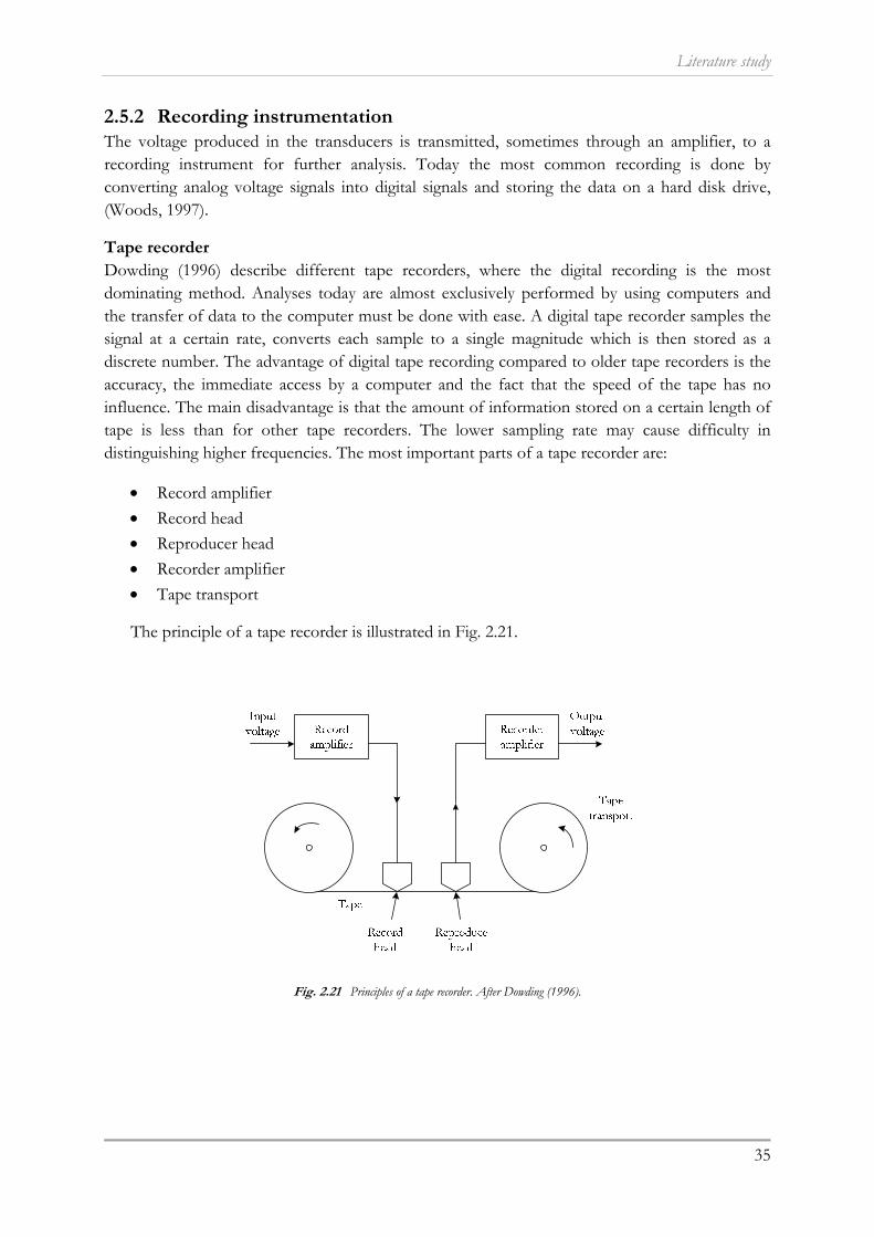
Literature study
35
2.5.2 Recording instrumentation The voltage produced in the transducers is transmitted, sometimes through an amplifier, to a recording instrument for further analysis. Today the most common recording is done by converting analog voltage signals into digital signals and storing the data on a hard disk drive, (Woods, 1997).
Tape recorder Dowding (1996) describe different tape recorders, where the digital recording is the most dominating method. Analyses today are almost exclusively performed by using computers and the transfer of data to the computer must be done with ease. A digital tape recorder samples the signal at a certain rate, converts each sample to a single magnitude which is then stored as a discrete number. The advantage of digital tape recording compared to older tape recorders is the accuracy, the immediate access by a computer and the fact that the speed of the tape has no influence. The main disadvantage is that the amount of information stored on a certain length of tape is less than for other tape recorders. The lower sampling rate may cause difficulty in distinguishing higher frequencies. The most important parts of a tape recorder are:
Record amplifier
Record head
Reproducer head
Recorder amplifier
Tape transport
The principle of a tape recorder is illustrated in Fig. 2.21.
Fig. 2.21 Principles of a tape recorder. After Dowding (1996).
Ground Vibrations due to Vibratory Sheet Pile Driving
36
Automatic systems Dunnicliff (1993) describes automatic data acquisition systems, which are programmed to collect data automatically, without human intervention. The data is either recorded immediately or retransmitted to other equipment for recording. Today the most common is to use either a data logger or a computer to record the vibration signals, (Measurement Computing, 2012).
A data logger is an instrument designed to record information from various transducers, usually at high speed. Data loggers are simpler than computers and more limited in storage capacity, but might be preferred when it is not practical to have a computer at the site.
A computer can be incorporated into the data acquisition system through the use of an interface device. Computers allow more sophisticated immediate data processing than a data logger. The interface device is often a plug-in card that can be easily connected to the computer by e.g. USB, PCI or Ethernet, (Measurement Computing, 2012).
The basic configuration of an automatic data acquisition system is that the analog output of transducers is converted into a signal that can be measured and converted into a digital number. The data is then stored or printed for further analysis, most commonly on the computer hard drive. Some systems can transmit data over the telephone network to a separate processing center.

Literature study
37
2.6 Prediction models There are several models developed for prediction of ground vibrations induced by sheet pile driving, with different levels of sophistication and difficulty. They range from simple empirical relations to advanced numerical models. This thesis is performed during a limited time period, why two simpler empirical models are chosen to study further. The models chosen are one of the first prediction models presented by Attewell and Farmer (1973) and a later developed model by Attewell et al. (1992), which is based on the first. Before presenting the models, some notes worth recognizing are mentioned.
The two models presented in this thesis are energy based. The input parameters are only the energy input of the vibratory equipment and the distance from the source. The energy input of a vibratory driver is expressed as the amount of energy per cycle given in Joules. A way to calculate the input energy is stated in Head and Jardine (1992). From the manufacturer the power input,
, and the rated frequency, , can be obtained. The energy per cycle is then given by Eq. (2.30).
1000 ∙
(2.30)
Where:
0= energy input [ J ] = power input [kW]
= frequency [Hz]
The distance from the source is the other input parameter in the prediction models. Massarsch and Fellenius (2008) states that this distance is not always well defined. Usually the horizontal distance along the ground surface is used, which might be misleading. Vibrations are emitted both from the shaft and the toe of the sheet pile and at a large penetration depth, there is quite a difference between the horizontal distance and the slope distance from the pile toe, see Fig. 2.22. Which length is used as distance from the source will affect the predicted vibration level.
Fig. 2.22 Difference between horizontal distance, r, and slope distance, s.

Ground Vibrations due to Vibratory Sheet Pile Driving
38
Hope and Hiller (2000) also argue for using the slope distance instead of the horizontal distance. Based on field measurements the authors find that the relationship between peak particle velocity and the horizontal distance from the pile is not linear. However, by instead using the slope distance from the pile toe to the point of observation, see Fig. 2.22, the distribution is more closely linear, according to Eq. (2.31).
∝1
(2.31)
= peak particle velocity [mm/s] = slope distance [m] = attenuation index [ - ]
2.6.1 Attewell and Farmer (1973) One of the earliest, most well known and most used empirical prediction models was developed by Attewell and Farmer (1973). The main conclusion of their study is that the reduction of the ground vibration amplitude in practical use can be estimated as independent of the geotechnical properties at the site and instead dependent only of the input energy of the pile driver and the distance from the source, according to Eq. (2.32). The authors reason that the losses due to material damping are very small relative the geometrical losses and that the attenuation process can be simplified to include only geometrical terms.
(2.32)
Where:
= predicted vertical velocity [mm/s] = constant of proportionality [ - ] = site specific constant [ - ] = input energy at source [ J ]
= horizontal distance from source [m] A linear regression analysis by least squares gave a best fit curve to their measured values according to Eq. (2.33).
0.76
.
(2.33)
It was also shown that all measured data fell below a curve with = 1.5 and = 1 and that all data except in one case fell below = 0.75. The authors suggested = 1.5 to be used in practice for conservative predictions of the vertical vibration amplitude.

Literature study
39
2.6.2 Attewell et al. (1992) The above presented model was later on developed into a new model, presented by Attewell, Selby and O’Donnell (1992a and 1992b). The analysis by Attewell et al. (1992) is statistical and based on the data obtained from Attewell and Farmer (1973) as well as new data from other field studies. The new model applies a quadratic fitting instead of a linear approximation of Attewell and Farmer (1973). The new model also takes special consideration to the difference between impact- and vibratory driving. Since the energy transmission from vibratory drivers is different from that of impact hammers, the authors state that vibration estimation needs to be considered differently. The empirical constants inserted into the model are decided based on the driving method. For vibratory driving, the quadratic relations according to Eq. (2.34)-(2.36) are given.
Best fit: log 0.464 1.64 log 0.334 log (2.34)
Half a standard deviation: log 0.213 1.64 log 0.334 log (2.35)
One standard deviation: log 0.038 1.64 log 0.334 log (2.36)
Attewell et al. (1992) recommends that vibration limits for normal construction work should be based on the one-half standard deviation curve, according to Eq. (2.35). The particle velocity to be used is still the vertical component of the vibration. The distance is not defined, but since the model is a development of Attewell and Farmer (1973), the same definition is assumed, i.e. the horizontal distance. The authors suggest the energy input stated by the manufacturer to be used since the losses at the pile are difficult to estimate.

Ground Vibrations due to Vibratory Sheet Pile Driving
40

Results and Analysis
41
3 Field study
3.1 Introduction An extension of the theatre building in Karlstad was planned, located according to Fig. 3.1, where Hercules Grundläggning AB were responsible for the foundation work. The theatre was constructed in 1893 and several buildings in the vicinity are also of older age, making the issue of environmental impact an important question. Hercules wanted to examine the possibility of installing sheet piles by vibratory driving, why NCC Teknik, in collaboration with Bergsäker, was asked to perform measurements and analysis of the environmental impact during a trial sheet piling where four sheet piles were driven with vibratory equipment on May 4, 2010. The decision was to not use vibratory driven sheet piles due to large settlements of the soil close to the sheet pile, but the measured vibrations were never closely analyzed.
The main part of this thesis consists of performing a deeper analysis of the measured vibration data from the field test in Karlstad, hopefully leading to a better understanding of the mechanisms behind the induced ground vibrations.
Fig. 3.1 Location of Karlstad theatre.

Ground Vibrations due to Vibratory Sheet Pile Driving
42
3.2 Description Following sections will provide insight to the field study. The geotechnical conditions at the site are described in the first section, followed by specifications of the driving- and measurement equipment. The section is concluded by a description of the measurement procedure.
3.2.1 Geotechnical conditions A geotechnical investigation was performed by Sweco, dated to 2006-05-02, which is the base of the estimated geotechnical conditions presented in this section. Several investigation points were placed around the theatre building, where five points close to the field study site are chosen to represent a characteristic section, C, of the soil profile. The characteristic section and the five points of interest, B_1, B_2, B_3, B_4 and B_5, are shown in Fig. 3.2. Sampling with helical auger was carried out at all points except B_2 where pressure sounding was performed. CPT-soundings were carried out at points B_1 and B_5, see Appendix A.1, (Sweco, 2006).
Fig. 3.2 Extract from plan drawing showing characteristic section and investigation points, (Sweco, 2006).
Based on the geotechnical investigation by Sweco (2006), a soil profile is estimated along the characteristic section. Fig. 3.3 illustrates the soil profile along with the setup of the measurement and driving equipment. The surface of paving stones is located at a level +47 m. Beneath the

Results and Analysis
43
paving stones is a layer of about 1.2 m fill material. This layer was at the time of the field study excavated at the area where the sheet piles were driven and the measurement equipment was setup, see also Fig. 3.7.
Underneath the fill material are natural deposits of loose fine grained river sediments, mainly sand with thin courses of mud and plant residues. The thickness of the sand layer is, in average along the section, 8 m. The sand then transitions into loose silt with courses of sand.
A sand layer of stiffer character is located at a depth of 11-12 m from the original surface level. Beneath this stiffer layer the soil consists of clay and silt for another 2 m.
At a depth of 14 m below the original surface level is a layer of moderately firm, glacial clay. The clay continues to a depth of 25 m below the surface. Properties of the clay were not further investigated during the geotechnical investigation. The modulus of elasticity of the clay is instead estimated according to Eq. (3.1), which is valid for normal consolidated clay.
150 ∙ (3.1) Where:
= modulus of elasticity [Pa] = undrained shear strength [Pa]
Below the clay is firm, frictional soil which was not further investigated. It was assumed to be a 0.5 – 1 m thick layer of moraine on rock. The bedrock level is estimated to +20.5 m.
The groundwater level was measured by installation of two observation pipes. These measurements showed a groundwater level at level +44.1 and +44.2, which is approximately 3 m below the ground surface.
Soil parameters are evaluated from the CPT-soundings as the average values along the profile. The shear modulus is calculated according to Eq. (2.8) and the Poisson ratio according to Tab. 2.1. The soil parameters are compiled in Tab. 3.1.
Tab. 3.1 Soil properties of the characteristic profile.
Layer Thickness [m]
[t/m3]
[MPa]
[MPa]
[ - ]
[ o]
[kPa]
Fill 1.2 1.75 Sand 7.7 1.80 19.1 7.6 0.25 36
Silt/sand 2.1 1.83 17.1 6.8 0.25 33 191Sand 1.0 1.96 33.5 13.4 0.25 36 Clay 1.1 1.87 12.7 4.4 0.45 85Silt 0.6 1.80 15.7 6.1 0.30 33 247Clay 12.1 1.75 7.0 2.4 0.45 46
Moraine 0.8
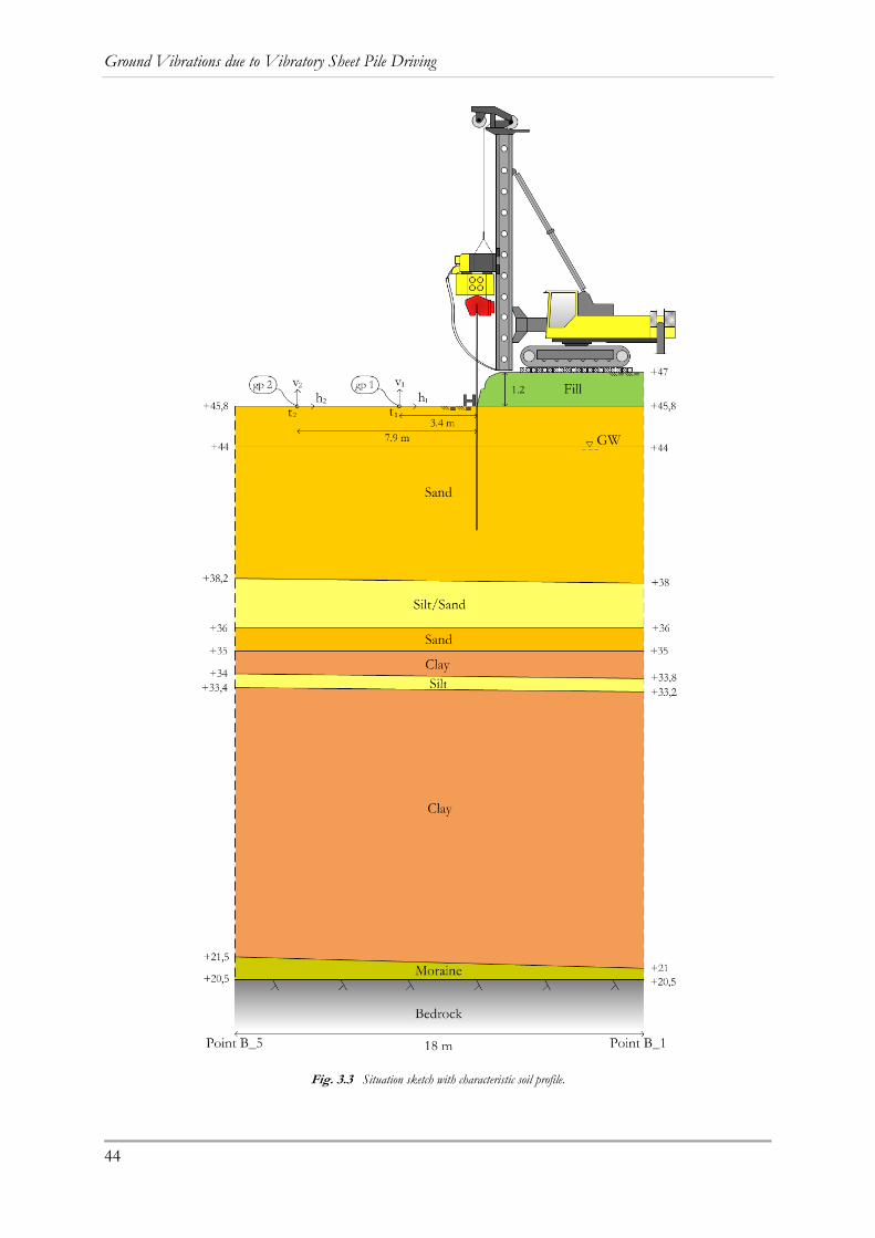
Ground Vibrations due to Vibratory Sheet Pile Driving
44
Fig. 3.3 Situation sketch with characteristic soil profile.

Results and Analysis
45
3.2.2 Driving equipment The driving equipment consisted of a variable frequency vibrator of type Dieseko 2316VM driven hydraulically by a power pack Dieseko PVE480, see Appendix A.2, for full specifications. The attachment to the carrier was a combination between a free hanging and leader mounted configuration, see Fig. 3.3 and Fig. 3.4. The vibrator itself is a free hanging model, but it was in this case mounted to a leader. The carrier was a Banut machine which also could be used for impact driving of piles and sheet piles.
Fig. 3.4 Driving equipment used at field measurement; power pack, vibrator unit and carrier. Photo by Kenneth Viking (2010).
Four sheet piles were used in the trial driving. The sheet piles were 12 m long of type PU12 and were driven to a depth of 10.5 – 11 m. Properties of the sheet pile are presented in Fig. 3.5 and in Tab. 3.2.
Fig. 3.5 Sheet pile profile PU12. Modified after ArcelorMittal (2012).
Tab. 3.2 Section properties for sheet pile profile PU12. After ArcelorMittal (2012).
Sectional area [cm2]
Mass per m [kg/m]
Moment of inertia [cm4]
Elastic section modulus [cm3]
Coating area [m2/m]
84.2 66.1 4500 370 0.80

Ground Vibrations due to Vibratory Sheet Pile Driving
46
3.2.3 Data acquisition The data acquisition equipment was provided by Bergsäker and consisted of two devices of type Ava95, see Fig. 3.6. This device includes several transducers; geophone, accelerometer and air pressure transducer, but geophones were used at this specific measurement. The Ava95 device has 4 recording channels and can register an event for up to 70 seconds. The sampling rate can be adjusted for different types of measurements and was at this field study chosen to 750 Hz. The measured data is recorded and automatically stored in a database, transferred from the device over the GSM network. The device has an internal storage of 1 GB, which is enough to store 3 to 4 measurement events. After this the memory needs to be cleared and the data transferred to the database, or the stored data will be overwritten. The transfer via the GSM network can take over an hour.
Fig. 3.6 The Ava95 system with the transducer in front and the recorder in the background. Photo by Kenneth Viking (2010).
The geophones used at this measurement where positioned at two different distances from the sheet pile line. The geophones were triaxial transducers, measuring in vertical, transversal and longitudinal direction. See Fig. 3.8 for direction definition. A third uniaxial geophone was placed at a further distance, measuring only maximum values of the vertical vibrations.
3.2.4 Measurement procedure Fig. 3.7 illustrates a plan sketch of the measurement site, showing driving equipment, measurement equipment, position of the sheet piles and the area where the fill layer was excavated. A magnification to clarify the measurement directions is illustrated in Fig. 3.8.
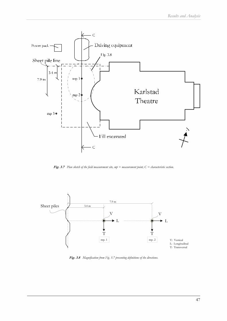
Results and Analysis
47
Fig. 3.7 Plan sketch of the field measurement site, mp = measurement point, C = characteristic section.
V
L
T
Sheet piles
V
T
3.4 m
7.9 m
L
V: VerticalL: LongitudinalT: Transversal
mp. 1 mp. 2
Fig. 3.8 Magnification from Fig. 3.7 presenting definitions of the directions.

Ground Vibrations due to Vibratory Sheet Pile Driving
48
Two triaxial geophones were placed at respectively 3.4 m and 7.9 m from the sheet pile line, see Fig. 3.7 - Fig. 3.9. The measurement points are further on referred to as mp. 1 and mp. 2, where mp. 1 is closest to the sheet pile line. One uniaxial geophone, measuring only maximum vertical values, was placed at about 15 m from the sheet pile line, referred to as mp. 3. To detect vibrations in the soil, the geophones were attached to 0.7 m long iron rods, inserted about 0.55 m into the ground. The geophones were attached at 0.1 m from the top of the rod, illustrated in Fig. 3.9.
Fig. 3.9 Left: Geophone setup at two distances from the sheet pile. Photo by Kenneth Viking (2010). Right: Geophone setup in the ground.
The measurements were initiated at the start of the sheet pile installation and continued during an interval of 70 seconds. However, the driving of the sheet piles lasted for a longer period than 70 seconds which means that the end of the process was not registered. The measurements were registered at a sampling frequency of 750 Hz.
To register the penetration depth and driving velocity of the sheet piles, chalk markings were placed every 10 cm on the sheet pile, with a larger mark at every meter. A video camera was placed about 10 m from the sheet pile line, filming the entire driving process. The idea was to get a third dimension to the measured values by being able to see at what time during the driving process certain values occur and perhaps also an explanation for unusual values.
Four sheet piles were driven during the trial, in order according to Fig. 3.10. Measurements were performed during the driving of the last three sheet piles, meaning that all measurements

Results and Analysis
49
correspond to driving the sheet pile into interlock with another profile. The sheet piles were driven to a depth of about 10.5 - 11 m, thus only entering the first layers of sand and silty sand.
Fig. 3.10 Driving order of the four sheet piles.
In the Results and Analysis section below, the numbering of the sheet piles is different since no measurement was performed during driving of the first sheet pile. Instead will sheet pile no. 1 correspond to the first measured sheet pile (sheet pile no. 2 in Fig. 3.10) and so forth, see Fig. 4.1.

Ground Vibrations due to Vibratory Sheet Pile Driving
50

Results and Analysis
51
4 Results and Analysis
4.1 Introduction The results from the field measurements in Karlstad are presented and analyzed to provide a better understanding and insight to the behavior of the induced ground vibrations. A comparison between the field results and the prediction models described in section 2.6 is also presented in this section.
4.2 Field study The following sections will present the results and analysis of the vibration measurements in Karlstad. The measured particle velocities are presented in different graphs, related to time, distance from source, penetration depth and resistance from the CPT-soundings. The frequency spectra of the vibrations are also studied.
Fig. 4.1 Denotation of sheet pile order.
There are some limitations considering the measurements, which must be acknowledged. Tab. 4.1 is a compilation of the measurements available for each driven sheet pile. The denotation of the sheet piles are also presented in Fig. 4.1.
Tab. 4.1 Available measurements for each sheet pile.
x : Yes : No
Sheet pile no. Interlock Measurement
point 1 Measurement
point 2 Penetration depth
estimation sp. 0 sp. 1 x x sp. 2 x x* x x** sp. 3 x x x x
* Not same time interval as mp. 2 ** Only valid for mp. 2

Ground Vibrations due to Vibratory Sheet Pile Driving
52
The penetration depth is estimated from the video recordings and chalk markings on the profiles. However, the triggering of the measurements is not visible in the videos, making an exact time synchronization between videos and measurements difficult. It is assumed that the measurements commence as the driving of the sheet pile commence, if otherwise not evident.
4.2.1 Particle velocity The particle velocity can be presented in different ways to describe the vibrations. The most common presentation is to plot the velocity against the time, where the vibration magnitudes also can be related to the video recordings. Plotted against distance from the source, the attenuation can be visualized. Plotted against the penetration depth and CPT results, they can be related to the properties of the soil. Typical results as well as points of interest are presented in following sections. More results are available in chapter 7, Appendix.
Time histories The most common presentation of vibrations is the time domain, see section (2.2.2), showing how the particle velocity varies with the elapsed time of measurement. The measurement of sheet pile no. 3 shows typical time histories. In mp. 1, the horizontal vibrations are of magnitude 10 mm/s, the transversal component somewhat larger than the longitudinal, while the vertical magnitude is less than 5 mm/s, see Fig. 4.2. In mp. 2 however, the vertical component is larger than the horizontal and slightly larger than in mp. 1. The horizontal vibrations have attenuated to well below 5 mm/s, see Fig. 4.3. The shapes of the curves correspond well to each other, where increases of the vibrations occur at the same time in all directions.
Time histories for the other sheet piles show the same trends with the largest vibrations in horizontal direction, at least close distance to the sheet pile, see Appendix A.3. It is not always expected that this will be the case and other field studies report the vertical vibrations to be the dominant component, especially at close distance to the sheet pile, e.g. Martin (1980), Viking et al. (2000), Ahlquist and Enggren (2006) and Whenham et al. (2009). As stated in section (2.4.5) a common relation is that the horizontal components are about 30-50 % of the vertical. Massarsch (2000) also stated that the horizontal components are larger in frictional soils and increase with the friction angle, which can be related to in this field study.
The soil at the site of the field study consisted of loose sand, which is also more prone to allow horizontal movement than a stiffer soil would. The driving equipment clamped the sheet piles by the web and not the neutral layer, hence applying the driving force eccentrically. The horizontal movement of the sheet pile due to the clamping in combination with the loose soil is a probable cause of the large horizontal vibrations.
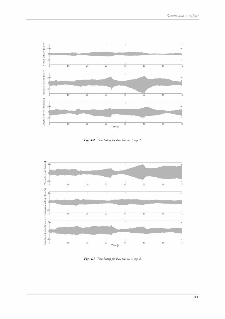
Results and Analysis
53
Fig. 4.2 Time history for sheet pile no. 3, mp. 1.
Fig. 4.3 Time history for sheet pile no. 3, mp. 2.

Ground Vibrations due to Vibratory Sheet Pile Driving
54
The vibratory driver produces a harmonic motion of the sheet pile. A magnification of the signals is presented in Fig. 4.4. At the closest distance to the sheet pile, the vertical component of the ground vibrations maintains the harmonic character, while the horizontal components do not. The signals in horizontal directions are instead periodic, containing other frequencies than the driving frequency. At a larger distance from the sheet pile, the vertical and transversal components are periodic while the longitudinal component is closer to harmonic.
19.8 19.85 19.9 19.95 20 20.05 20.1 20.15 20.2-4
-2
0
2
4
Ver
tical
vel
ocity
[mm
/s]
19.8 19.85 19.9 19.95 20 20.05 20.1 20.15 20.2-10
-5
0
5
10
Tra
nsve
rsal
vel
ocity
[mm
/s]
19.8 19.85 19.9 19.95 20 20.05 20.1 20.15 20.2-10
-5
0
5
10
Time [s]Lon
gitu
dina
l vel
ocity
[mm
/s]
19.8 19.85 19.9 19.95 20 20.05 20.1 20.15 20.2-4
-2
0
2
4
Ver
tical
vel
ocity
[mm
/s]
19.8 19.85 19.9 19.95 20 20.05 20.1 20.15 20.2-4
-2
0
2
4
Tra
nsve
rsal
vel
ocity
[mm
/s]
19.8 19.85 19.9 19.95 20 20.05 20.1 20.15 20.2-4
-2
0
2
4
Time [s]Lon
gitu
dina
l vel
ocity
[mm
/s]
Fig. 4.4 Magnification of signals from sheet pile no. 3. a) mp. 1 b) mp. 2
A time history of less typical character was obtained during the measurement of sheet pile no. 2 at mp. 1, see Fig. 4.5. The measurement in mp. 1 begins 83 s after mp. 2 and measures the end of the driving procedure. During the 70 s of this measurement, the sheet pile is driven to the final depth of 11 m, immediately extracted about 1 m, after which it is driven down to 11 m again.
The recordings show exceptionally large vibrations, compared to the other measurements. The particle velocity in the longitudinal direction exceeds the limit value of the recording device of 27 mm/s. It would have been interesting to see how much these large vibrations attenuate to the second measurement point, but unfortunately mp. 2 does not measure the same time period. However, the origin of these large vibrations is still interesting and will be discussed further.

Results and Analysis
55
Fig. 4.5 Time history for sheet pile no. 2, mp. 1.
A close-up on the longitudinal component alone is presented in Fig. 4.6, along with some comments explaining the driving procedure captured by this measurement. The first 12 s of measurement correspond to both driving and extracting, around the depth 10.5 – 11 m. The vibrations are large, but quite similar in magnitude. The extraction after the 16 s stop produces vibrations of the same order of magnitude. When the downward driving is resumed at 35 s into the measurement, the vibration magnitude increases and soon reaches the limit of 27 mm/s. The driving velocity is very slow, driving only 1 m in 30 s, much slower than driving the same path during the first 4 s of measurement.
Fig. 4.6 Longitudinal vibration, sheet pile no. 2, mp.1, with comments.
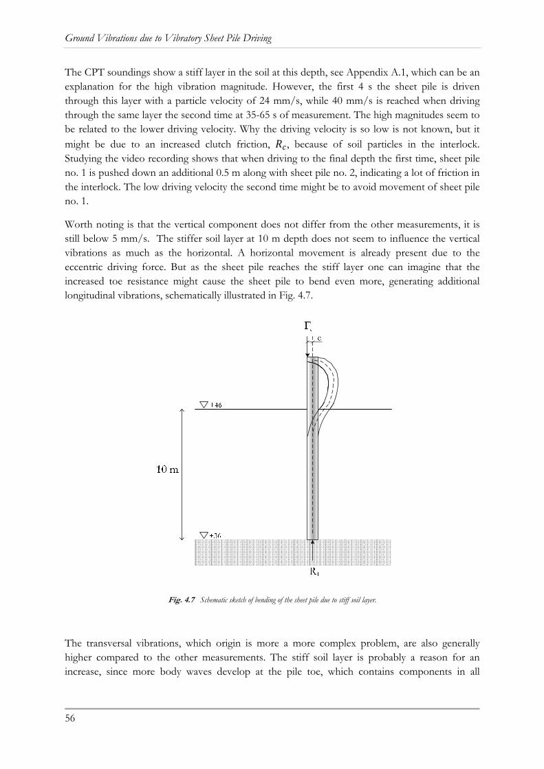
Ground Vibrations due to Vibratory Sheet Pile Driving
56
The CPT soundings show a stiff layer in the soil at this depth, see Appendix A.1, which can be an explanation for the high vibration magnitude. However, the first 4 s the sheet pile is driven through this layer with a particle velocity of 24 mm/s, while 40 mm/s is reached when driving through the same layer the second time at 35-65 s of measurement. The high magnitudes seem to be related to the lower driving velocity. Why the driving velocity is so low is not known, but it might be due to an increased clutch friction, , because of soil particles in the interlock. Studying the video recording shows that when driving to the final depth the first time, sheet pile no. 1 is pushed down an additional 0.5 m along with sheet pile no. 2, indicating a lot of friction in the interlock. The low driving velocity the second time might be to avoid movement of sheet pile no. 1.
Worth noting is that the vertical component does not differ from the other measurements, it is still below 5 mm/s. The stiffer soil layer at 10 m depth does not seem to influence the vertical vibrations as much as the horizontal. A horizontal movement is already present due to the eccentric driving force. But as the sheet pile reaches the stiff layer one can imagine that the increased toe resistance might cause the sheet pile to bend even more, generating additional longitudinal vibrations, schematically illustrated in Fig. 4.7.
Fig. 4.7 Schematic sketch of bending of the sheet pile due to stiff soil layer.
The transversal vibrations, which origin is more a more complex problem, are also generally higher compared to the other measurements. The stiff soil layer is probably a reason for an increase, since more body waves develop at the pile toe, which contains components in all

Results and Analysis
57
directions. Another possible reason could be an increase of the clutch friction, as mentioned above. acts only on one side of the sheet pile and, if increased, will cause an uneven driving. If the sheet pile is constrained more on one side than the other, it will bend and twist. This might cause additional vibrations in both longitudinal and transversal directions. The clutch friction is affected by soil particles in the interlocks and by the condition of the interlocks, but also very much by the operator of the machinery. If the sheet piles aren’t properly aligned and driven with precision as they are driven into interlock, the clutch friction is increased.
Maximum vibration level The maximum values of the vibration magnitude are in many cases the point of interest. The particle velocities at each measurement, each observation point and in each direction are compiled in Tab. 4.2.
Tab. 4.2 Maximum velocity of each measured direction at the two observation points.
Sheet pile no.
Direction vmax at mp. 1 [mm/s]
(distance 3.4 m) vmax at mp. 2 [mm/s]
(distance 7.9 m) vmax at mp. 3 [mm/s]
(distance 15 m)
1 Vertical 3.4 - 1.6 Transversal 9.9 - - Longitudinal 18.9 - -
2 Vertical 3.8* 6.3 2.1 Transversal 15.9* 3.9 - Longitudinal 27.8* 4.9 -
3 Vertical 4.1 5.1 1.5 Transversal 17.2 2.3 - Longitudinal 10.0 3.3 -
* Not measured in the same time interval as mp. 2
Attenuation The attenuation of the vibrations is visualized by plotting the particle velocity against the distance from the source of vibration. As sheet pile no. 3 is the only measurement representing the same time period in both measurement points, only this one can be used to present the attenuation of vibration velocity between mp. 1 and mp. 2. The attenuation is shown in Fig. 4.8, with the maximum values of each measured direction, as well as the peak particle velocity, . It can be concluded that even the large magnitudes in horizontal direction attenuates rather quickly to values below 5 mm/s at a distance of about 8 m from the source.
The transversal and longitudinal direction shows a larger magnitude in mp. 1, as well as the , while the vertical vibrations actually have larger magnitudes in mp. 2. The vertical direction was also measured in mp. 3, where it is evident that also the vertical vibrations decrease with distance.
The fact that the vertical vibrations are larger at the longer distance from the sheet pile can be explained. Since waves are developed both along the shaft and at the toe of the sheet pile, the waves will travel different distances, and with different velocities, before they reach the measurement points. Refraction and reflection mechanisms will also change the characteristics of
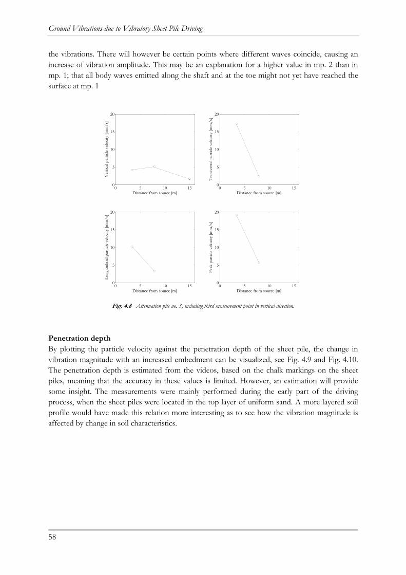
Ground Vibrations due to Vibratory Sheet Pile Driving
58
the vibrations. There will however be certain points where different waves coincide, causing an increase of vibration amplitude. This may be an explanation for a higher value in mp. 2 than in mp. 1; that all body waves emitted along the shaft and at the toe might not yet have reached the surface at mp. 1
Fig. 4.8 Attenuation pile no. 3, including third measurement point in vertical direction.
Penetration depth By plotting the particle velocity against the penetration depth of the sheet pile, the change in vibration magnitude with an increased embedment can be visualized, see Fig. 4.9 and Fig. 4.10. The penetration depth is estimated from the videos, based on the chalk markings on the sheet piles, meaning that the accuracy in these values is limited. However, an estimation will provide some insight. The measurements were mainly performed during the early part of the driving process, when the sheet piles were located in the top layer of uniform sand. A more layered soil profile would have made this relation more interesting as to see how the vibration magnitude is affected by change in soil characteristics.
0 5 10 150
5
10
15
20
Distance from source [m]
Ver
tical
par
ticle
vel
ocity
[mm
/s]
0 5 10 150
5
10
15
20
Distance from source [m]
Tra
nsve
rsal
par
ticle
vel
ocity
[mm
/s]
0 5 10 150
5
10
15
20
Distance from source [m]
Lon
gitu
dina
l par
ticle
vel
ocity
[mm
/s]
0 5 10 150
5
10
15
20
Distance from source [m]
Pea
k pa
rtic
le v
eloc
ity [m
m/s
]
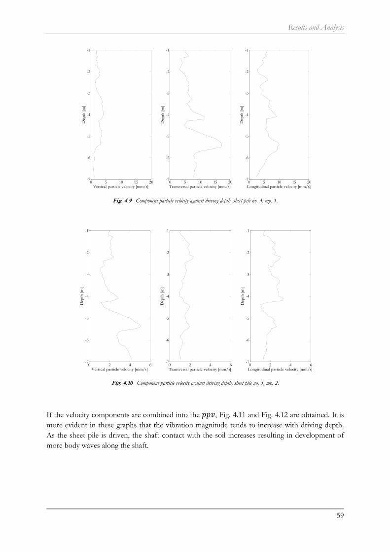
Results and Analysis
59
Fig. 4.9 Component particle velocity against driving depth, sheet pile no. 3, mp. 1.
Fig. 4.10 Component particle velocity against driving depth, sheet pile no. 3, mp. 2.
If the velocity components are combined into the , Fig. 4.11 and Fig. 4.12 are obtained. It is more evident in these graphs that the vibration magnitude tends to increase with driving depth. As the sheet pile is driven, the shaft contact with the soil increases resulting in development of more body waves along the shaft.
0 5 10 15 20-7
-6
-5
-4
-3
-2
-1
Vertical particle velocity [mm/s]
Dep
th [m
]
0 5 10 15 20-7
-6
-5
-4
-3
-2
-1
Transversal particle velocity [mm/s]
Dep
th [m
]
0 5 10 15 20-7
-6
-5
-4
-3
-2
-1
Longitudinal particle velocity [mm/s]
Dep
th [m
]
0 2 4 6-7
-6
-5
-4
-3
-2
-1
Vertical particle velocity [mm/s]
Dep
th [m
]
0 2 4 6-7
-6
-5
-4
-3
-2
-1
Transversal particle velocity [mm/s]
Dep
th [m
]
0 2 4 6-7
-6
-5
-4
-3
-2
-1
Longitudinal particle velocity [mm/s]
Dep
th [m
]

Ground Vibrations due to Vibratory Sheet Pile Driving
60
0 5 10 15 20-7
-6
-5
-4
-3
-2
-1
Peak particle velocity [mm/s]
Dep
th [m
]
0 2 4 6-7
-6
-5
-4
-3
-2
-1
Peak particle velocity [mm/s]D
epth
[m]
CPT resistance The particle velocity is plotted against the soil resistance obtained from the CPT soundings in the geotechnical investigation, to see if any correlation exists. The main conclusion is that some correlation can be found, but not consequently in all measurements. There are several uncertainties in this specific field study, making it difficult to evaluate if there truly are correlations or if they only appear by chance.
The best correlation is found in the measurement of sheet pile no. 3, see Appendix A.4 for the other measurements. In the figures below, the sleeve resistance from investigation point B_5 is used, see also Fig. 3.2. At closest distance to the sheet pile, Fig. 4.13, the horizontal particle velocities seem to be more correlated to the sleeve resistance than the vertical component. The maximum value of the vibration magnitude corresponds to a peak in the soil resistance. This is however not the case for the vertical vibration. At the larger distance, Fig. 4.14, the opposite seems to appear. The peak in the vertical vibration amplitude corresponds with the soil resistance, while the horizontal does not.
Considering the fact that the correlation is found in some cases and in some cases not at all, suggests that the soil resistance do influence the vibration magnitude, but not on its own. It is found that where there are peaks in the soil resistance, there are often also peaks in the particle velocity, indicating that firmer layers give rise to larger vibration amplitudes. However, this is not always the case. Large vibration amplitudes are also found where the resistance is low, indicating that other factors may be more decisive for the magnitude of vibration. Important to note is also that the penetration depth for the vibration measurements are not exact, only estimated.
Fig. 4.11 Peak particle velocity, pile no. 3, mp. 1 Fig. 4.12 Peak particle velocity, pile no. 3, mp. 2.

Results and Analysis
61
Fig. 4.13 CPT resistance vs. particle velocity, sheet pile no. 3, mp. 1.
Fig. 4.14 CPT resistance vs. particle velocity, sheet pile no. 3, mp. 2.
0 2 4 6-7
-6
-5
-4
-3
-2
-1
Vertical velocity [mm/s]
Dep
th [m
]0 20 40 60
-7
-6
-5
-4
-3
-2
-1
Sleeve friction [kPa]
0 5 10 15 20-7
-6
-5
-4
-3
-2
-1
Transversal velocity [mm/s]
0 20 40 60
-7
-6
-5
-4
-3
-2
-1
Sleeve friction [kPa]
0 5 10 15-7
-6
-5
-4
-3
-2
-1
Longitudinal velocity [mm/s]
0 20 40 60
-7
-6
-5
-4
-3
-2
-1
Sleeve friction [kPa]
Particle velocityCPT resistance
0 2 4 6-7
-6
-5
-4
-3
-2
-1
Vertical velocity [mm/s]
Dep
th [m
]
0 20 40 60
-7
-6
-5
-4
-3
-2
-1
Sleeve friction [kPa]
0.5 1 1.5 2 2.5-7
-6
-5
-4
-3
-2
-1
Transversal velocity [mm/s]
0 20 40 60
-7
-6
-5
-4
-3
-2
-1
Sleeve friction [kPa]
1 2 3 4-7
-6
-5
-4
-3
-2
-1
Longitudinal velocity [mm/s]
0 20 40 60
-7
-6
-5
-4
-3
-2
-1
Sleeve friction [kPa]
Particle velocityCPT resistance

Ground Vibrations due to Vibratory Sheet Pile Driving
62
Particle motion To visualize the motion of the particles within the propagating wave, the particle velocity in different directions can be plotted against each other. The figures below show the particle motion during a time period of 1 s during the driving of sheet pile no. 3. See Appendix A.5 for the other measurements.
At closest distance to the sheet piles, Fig. 4.15 is obtained. The motion pattern is rather irregular, which is logical since at this distance both body waves and surface waves will interact and influence the particle motion.
The particle motion further from the sheet pile shows a better defined movement, Fig. 4.16, with a mainly vertical motion in the transversal plane and an ellipsoidal motion in the longitudinal plane. This pattern is typical for Rayleigh waves; an ellipsoidal motion in the direction of propagation. Since body waves attenuate faster than surface waves, Rayleigh waves are likely to be the dominating wave type at this distance from the sheet pile.
Fig. 4.15 Particle motion during driving of sheet pile no. 3, mp. 1.
Fig. 4.16 Particle motions during driving of sheet pile no. 3, mp. 2.
-6 -4 -2 0 2 4 6-6
-4
-2
0
2
4
6
Transversal velocity [mm/s]
Ver
tical
vel
ocity
[mm
/s]
-6 -4 -2 0 2 4 6-6
-4
-2
0
2
4
6
Longitudinal velocity [mm/s]
Ver
tical
vel
ocity
[mm
/s]
-3 -2 -1 0 1 2 3-3
-2
-1
0
1
2
3
Transversal velocity [mm/s]
Ver
tical
vel
ocity
[mm
/s]
-3 -2 -1 0 1 2 3-3
-2
-1
0
1
2
3
Longitudinal velocity [mm/s]
Ver
tical
vel
ocity
[mm
/s]

Results and Analysis
63
A three dimensional presentation of the particle movement can be obtained by plotting all components against each other. The Rayleigh wave pattern in mp. 2 with a mainly ellipsoidal movement in the longitudinal direction is presented in Fig. 4.17.
Fig. 4.17 Three dimensional presentation of the particle motion during driving of sheet pile no. 3, in mp. 2.
4.2.2 Frequency By using the Fast Fourier Transform function in Matlab, the frequency spectra are obtained, see Fig. 4.18 -Fig. 4.19. The y-axis corresponds to the vibration amplitude. The values can be compared to Tab. 4.2, where in mp. 1 the amplitude is smallest in vertical direction and largest in transversal direction and in mp. 2 the opposite situation. All frequency spectra can be found in Appendix A.6.
The dominant frequency is corresponding to the driving frequency, which for sheet pile no. 3 is 28 Hz. The smaller peaks in the spectra represent the other natural frequencies of the system, showing up at equal distance with the spacing of the driving frequency, in this case 28 Hz.
-3-2
-10
12
3
-3-2
-10
12
3-3
-2
-1
0
1
2
3
TransversalLongitudinal
Ver
tical

Ground Vibrations due to Vibratory Sheet Pile Driving
64
Fig. 4.18 Frequency spectra of all directions, sheet pile no. 3, mp. 1.
Fig. 4.19 Frequency spectra of all directions, sheet pile no. 3, mp. 2.
It is evident that the horizontal vibrations contain higher frequencies than the vertical. This was also recognized by Svinkin (1996) and Whenham et al. (2009), as mentioned in section (2.4.5). If the energy content of the signals instead of vibration amplitude is plotted on the y-axis, Fig. 4.20 - Fig. 4.22 are obtained. The energy content shows how many of the recorded vibrations that contain a certain frequency. It is evident that 100 % of the vibrations contain the dominant driving frequency while a lower percentage is periodic, containing higher frequencies as well. In these graphs it is clearer that the horizontal components contain more higher frequencies. It appears that the transversal frequency content, Fig. 4.21, is larger than the longitudinal, Fig. 4.22.
0 20 40 60 80 100 120
0
2
4
6
8
10
12
14
16
18Vertical
Frequency [Hz]
Par
ticle
vel
ocity
[mm
/s]
0 20 40 60 80 100 120
0
2
4
6
8
10
12
14
16
18Transversal
Frequency [Hz]
Par
ticle
vel
ocity
[mm
/s]
0 20 40 60 80 100 120
0
2
4
6
8
10
12
14
16
18Longitudinal
Frequency [Hz]
Par
ticle
vel
ocity
[mm
/s]
0 20 40 60 80 100 120-1
0
1
2
3
4
5
6Vertical
Frequency [Hz]
Par
ticle
vel
ocity
[mm
/s]
0 20 40 60 80 100 120-1
0
1
2
3
4
5
6Transversal
Frequency [Hz]
Par
ticle
vel
ocity
[mm
/s]
0 20 40 60 80 100 120-1
0
1
2
3
4
5
6Longitudinal
Frequency [Hz]
Par
ticle
vel
ocity
[mm
/s]
Results and Analysis
65
Fig. 4.20 Vertical component, sheet pile no. 3, mp. 2.
Fig. 4.21 Transversal component, sheet pile no. 3, mp. 2.
Fig. 4.22 Longitudinal component, sheet pile no. 3, mp. 2.

Ground Vibrations due to Vibratory Sheet Pile Driving
66

Results and Analysis
67
4.3 Prediction models The prediction models described in section (2.6) considers only the vertical component of the vibrations. The maximum vertical velocities from the field study are inserted into the models and then compared with the actual values. The two studied prediction models are energy based, with the energy input of the vibratory equipment and the distance from the source as input parameters. The energy input can be calculated according to Eq. (2.30), given the power input and frequency of the vibrator. The specification states a maximum hydraulic power of 250 kW. To get a slightly more accurate estimation of the energy input, the actual driving frequency is used instead of the rated frequency from the specifications, which was 38 Hz. The driving frequency was in this case 30 Hz. The energy input can then be calculated as:
1000 ∙ 1000 ∙ 25030
8.3
Important to note is that the energy is still the theoretical energy input of the vibrator. In reality there will be losses, causing the energy amount to differ from what the vibrator produces to what is actually transmitted to generate vibrations. This is not considered in the comparison below, which leads to higher vibration estimations than if the actual energy input could be used.
4.3.1 Attewell and Farmer (1973) Attewell and Farmer (1973) present a model based on Eq. (2.32) and give examples of constants for the best fit line of their data as well as for a conservative estimation of vibration magnitude. The input parameters in the model are the given empirical constants, distance from the sheet pile and the energy input of the vibrator used in the specific field study, which was above calculated to 8.3 kJ. The predicted particle velocities from the model together with the measured vibrations are presented in Fig. 4.23.
Fig. 4.23 Max. vertical velocity of field measurements compared to Attewell and Farmer (1973) model.
2 4 6 8 10 12 14 160
5
10
15
20
25
30
35
40
45
50
Horizontal distance [m]
Ver
tica
l par
ticle
vel
ocity
[mm
/s]
Best fit, k = 0.76, m = 0.87Conservative, k = 1.5, m = 1Pile 1Pile 2Pile 3
Ground Vibrations due to Vibratory Sheet Pile Driving
68
Both the conservative prediction and the best fit line are well above all field measurements. The overestimation is very large, especially close to the sheet pile. It appears that the attenuation is non-linear, at least close to the sheet pile, since the vibration amplitude in both mp. 1 and mp. 3 are lower than in mp. 2.
The maximum vertical velocity for several measurements occurs at a depth of around 5.5 m. The exception is mp.1 during driving of pile no. 2, where the measurement began at about 10 m penetration depth. By instead of the horizontal distance using the slope distance from the pile toe at this penetration depth, as suggested by Hope and Hiller (2000), Fig. 4.24 is obtained. The predicted magnitudes when using the slope distance are still overestimated. The overestimation is however reduced, compared to using the horizontal distance.
Fig. 4.24 Attewell and Farmer (1973) model with slope distance at penetration depth 5.5 m.
The best fit line for the field measurement data is presented in Fig. 4.25. By using the equation form of Attewell and Farmer (1973), Eq. (4.1) is obtained.
0.48
.
(4.1)
6 8 10 12 14 16 180
5
10
15
20
25
Slope distance [m]
Ver
tica
l par
ticl
e ve
loci
ty [m
m/s
]
Best fit, k = 0.76, m = 0.87Conservative, k = 1.5, m = 1Pile 1Pile 2Pile 3

Results and Analysis
69
Fig. 4.25 Best fit line for measurement data, with k = 0.48 and m = 0.6.
4.3.2 Attewell et al. 1992 The previous model was developed into to a new model presented by Attewell et al. (1992). The input parameters are the same, with given statistically obtained constants, distance from the sheet pile and energy input of the vibrator. In the new model, the non-linear attenuation is considered by applying quadratic prediction curves instead of linear, see Eq. (2.34)-(2.36). The result is shown in Fig. 4.26.
Fig. 4.26 Max. vertical velocity of field measurements compared to Attewell et al. (1992) model.
2 4 6 8 10 12 14 161
2
3
4
5
6
7
Horizontal distance [m]
Ver
tica
l par
ticle
vel
ocit
y [m
m/s
]
0 2 4 6 8 10 12 14 161
2
3
4
5
6
7
8
Horizontal distance [m]
Ver
tical
par
ticle
vel
ocity
[mm
/s]
One standard deviation
Half a standard deviation
Best fit
Pile 1
Pile 2
Pile 3

Ground Vibrations due to Vibratory Sheet Pile Driving
70
This model provides a better estimation of the vibration magnitudes, with less overestimation in general and much more accurate at the closest measurement point. At a larger distance, in mp. 3, the vibrations are however still over estimated. Attewell et al. (1992) suggest the half a standard deviation curve to be used for normal construction work. All measured values fall below this line except for pile no. 2 at mp. 2.
By using the slope distance from the pile toe instead of the horizontal distance, Fig. 4.27 is obtained. It is evident that in this model, the difference in predicted magnitudes by using different distances to source is insignificant.
Fig. 4.27 Attewell et al. (1992) model with slope distance at penetration depth 5.5 m.
4 6 8 10 12 14 16 181
2
3
4
5
6
7
8
Slope distance [m]
Ver
tical
par
ticle
vel
ocity
[mm
/s]
One standard deviation
Half a standard deviation
Best fit
Pile 1
Pile 2
Pile 3

Results and Analysis
71
4.4 Discussion The main findings and reflections concerning the field study and the evaluation of the prediction models are discussed in this section.
4.4.1 Field study Several uncertainties are related to the field measurements in Karlstad, where some measurements were faulty, some was not performed during the same time period in both measurement points and it was difficult to accurately estimate at what depth the sheet pile was located during the measurements. Still, the field study provides a lot of results worth discussing to increase the understanding of the induced ground vibrations.
Horizontal vibrations The most interesting point from the results of the field study is the magnitude of the horizontal vibration components, which are not generally expected to be larger than the vertical component. The waves generated at the sheet pile toe and shaft are known to include components of all directions, but not necessarily with this ratio. Since the motion induced by the vibratory driver is in vertical direction, the origin of the horizontal components is an interesting topic. It is discussed that the configuration of clamping the sheet pile by the web, beside the neutral layer of the profile, cause horizontal movement which in turn generate additional longitudinal vibrations. Clutch friction due to soil particles in the interlock is another factor which might increase the vibrations.
It is also found that the vertical vibrations are of relatively harmonic character, which is produced by the vibratory driver. The horizontal vibrations are however of period character and has larger content of higher frequency overtones, but still with the dominating frequency of the driving frequency.
Human errors The skill of the person operating the machinery is also of importance. Additional vibrations might be generated if different unwanted movements of the sheet pile are introduced. For example if the sheet pile is not properly aligned with the profile to which it is driven into interlock with. This would increase the clutch friction and thus the vibrations.
Soil characteristics Site specific soil properties also influence the vibration magnitude, but mainly the horizontal components. The loose sand in Karlstad allows the sheet pile to move more easily in horizontal direction than a stiffer soil would. The soil influence is also evident as the sheet pile reaches a stiffer sand layer at a larger depth, which generates an increase in horizontal (mainly longitudinal) direction. The vibrations in vertical direction were however unaffected. The stiff layer might cause the sheet pile to bend in longitudinal direction and hence increase the vibration level.
Even though the horizontal vibrations are quite large at a close distance to the sheet pile, they attenuate rather quickly to values below 5 mm/s at the second measurement point at distance 8 m, which at that point shows a particle motion typical for Rayleigh waves. It would have been

Ground Vibrations due to Vibratory Sheet Pile Driving
72
interesting to see if the same attenuation was achieved as the sheet pile reached the stiff soil layer, since it is theoretically known that waves attenuates slower in stiffer layers, but this measurement was only performed in mp. 1.
Relating to penetration depth The presentations where vibration magnitudes are related to penetration depth are the most uncertain results in this field study. The depth is estimated from videos which are difficult to synchronize with the measurements. Penetration depth is however an interesting parameters, in order to relate to the soil profile. The results show a trend of increasing vibration magnitude with increasing penetration depth, which can be expected due to larger contact area between sheet pile and soil. The vibration magnitudes are also plotted together with results from CPT soundings but, at least in this field study, a correlation is difficult to distinguish. Other measurements with more reliable depth indicator might give better results.
4.4.2 Prediction models The basic conclusion from the comparison between the measured field results and the prediction models are that the vibration magnitude is overestimated by the models. Even though prediction models usually are developed to overestimate the vibrations, to include some level of safety, the over estimation is quite large in this comparison. Very much in the earlier model and mostly at a further distance from the sheet pile in the later developed model.
It is important to acknowledge that empirical models are always accompanied with uncertainty since the result from the models will give reasonable values only of the site characteristics of the specific field study are similar to the site on which the empirical model is based.
Another limitation of the models studied is the input parameters which are the energy input of the vibratory driver and the distance from the source. The energy input is taken as the specified maximum capacity, with no regard to energy losses in the different transfers from vibrator to soil. This will cause an overestimation of the model results. The distance to the source is also a parameter which can be discussed. The Attewell and Farmer (1973) model shows a better result when using the slope distance to the source instead of the horizontal distance along the ground, while there is no difference between the two distances in the Attewell et al. (1992) model.
It can be concluded that the quadratic model by Attewell et al. (1992) provides a better agreement than the linear model by Attewell and Farmer (1973). It may not be quite as simple to use but still rather easy to handle. The input parameters are the same, with other constants to apply. Attewell et al. (1992) makes a difference between impact drivers and vibratory drivers, which is good since the energy transmission is quite different between the two methods.
A quadratic relation describing the attenuation of vibration amplitude is better than a linear, at least when studying the vertical component. The horizontal components seem to attenuate more linearly, at least in this specific field study. Suggestions for the development of a new prediction model are to incorporate the losses from the produced energy to the energy actually used to transmit vibrations to the soil and to acknowledge the site specific soil conditions, which in the field study have been shown to influence the vibration magnitude

Conclusions
73
5 General conclusions and proposal for further research
5.1 Conclusions A study of ground vibrations induced by vibratory sheet pile driving has been presented. During the course of completing this thesis, the main focus has been on interpreting and analyzing the recorded measurement data from the field test in Karlstad. The aim stated in the beginning of the thesis was to contribute to the understanding of induced ground vibrations and their propagation through the soil. This field study, even though it is quite limited, provides some interesting results. Simple empirical prediction models, as the two studied in this thesis, are known to give quite rough estimations of the vibration magnitudes. The results obtained by the comparison in this thesis is basically just another confirmation of this fact; that simple empirical models not taking the characteristics of the soil into account are very crude and overestimates the vibration magnitude.
The main conclusions drawn from this study are:
The results from the field study show that the focus of vibration analysis should not necessarily always be the vertical vibration components. Different factors can cause the horizontal vibration components to be of larger magnitude than the vertical.
The vibratory equipment produces a harmonic, vertical motion of the sheet pile. The waves generated propagate with components in both vertical and horizontal directions. Horizontal movements of the sheet pile might be introduced, e.g. by the configuration of the driving equipment, which will generate additional vibrations in horizontal directions. A different clamping of the sheet pile profiles where the force is applied in the neutral layer of the sheet pile would decrease horizontal movement.
The soil characteristics influence the magnitude of the vibrations. The loose sand in Karlstad provides less resistance to horizontal movements of the sheet pile. As the sheet pile reaches a stiffer soil layer, the vibration magnitude increases. The increase is most apparent in the longitudinal direction because the increase in toe resistance will cause the sheet pile to bend in that direction.
For empirical models to provide a good estimation, the site conditions must be similar to the ones the model is based on. A model such as Attewell et al. (1992) which is based on several field tests with different soil conditions provides a better estimation.
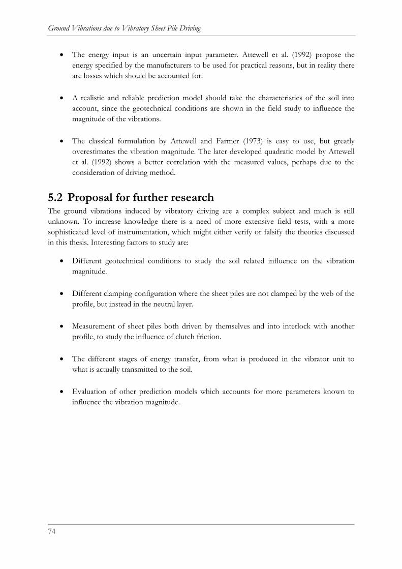
Ground Vibrations due to Vibratory Sheet Pile Driving
74
The energy input is an uncertain input parameter. Attewell et al. (1992) propose the energy specified by the manufacturers to be used for practical reasons, but in reality there are losses which should be accounted for.
A realistic and reliable prediction model should take the characteristics of the soil into account, since the geotechnical conditions are shown in the field study to influence the magnitude of the vibrations.
The classical formulation by Attewell and Farmer (1973) is easy to use, but greatly overestimates the vibration magnitude. The later developed quadratic model by Attewell et al. (1992) shows a better correlation with the measured values, perhaps due to the consideration of driving method.
5.2 Proposal for further research The ground vibrations induced by vibratory driving are a complex subject and much is still unknown. To increase knowledge there is a need of more extensive field tests, with a more sophisticated level of instrumentation, which might either verify or falsify the theories discussed in this thesis. Interesting factors to study are:
Different geotechnical conditions to study the soil related influence on the vibration magnitude.
Different clamping configuration where the sheet piles are not clamped by the web of the profile, but instead in the neutral layer.
Measurement of sheet piles both driven by themselves and into interlock with another profile, to study the influence of clutch friction.
The different stages of energy transfer, from what is produced in the vibrator unit to what is actually transmitted to the soil.
Evaluation of other prediction models which accounts for more parameters known to influence the vibration magnitude.
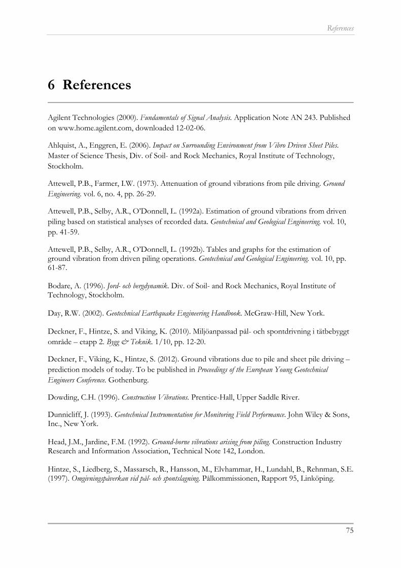
References
75
6 References
Agilent Technologies (2000). Fundamentals of Signal Analysis. Application Note AN 243. Published on www.home.agilent.com, downloaded 12-02-06.
Ahlquist, A., Enggren, E. (2006). Impact on Surrounding Environment from Vibro Driven Sheet Piles. Master of Science Thesis, Div. of Soil- and Rock Mechanics, Royal Institute of Technology, Stockholm.
Attewell, P.B., Farmer, I.W. (1973). Attenuation of ground vibrations from pile driving. Ground Engineering. vol. 6, no. 4, pp. 26-29.
Attewell, P.B., Selby, A.R., O’Donnell, L. (1992a). Estimation of ground vibrations from driven piling based on statistical analyses of recorded data. Geotechnical and Geological Engineering. vol. 10, pp. 41-59.
Attewell, P.B., Selby, A.R., O’Donnell, L. (1992b). Tables and graphs for the estimation of ground vibration from driven piling operations. Geotechnical and Geological Engineering. vol. 10, pp. 61-87. Bodare, A. (1996). Jord- och bergdynamik. Div. of Soil- and Rock Mechanics, Royal Institute of Technology, Stockholm. Day, R.W. (2002). Geotechnical Earthquake Engineering Handbook. McGraw-Hill, New York. Deckner, F., Hintze, S. and Viking, K. (2010). Miljöanpassad pål- och spontdrivning i tätbebyggt område – etapp 2. Bygg & Teknik. 1/10, pp. 12-20.
Deckner, F., Viking, K., Hintze, S. (2012). Ground vibrations due to pile and sheet pile driving – prediction models of today. To be published in Proceedings of the European Young Geotechnical Engineers Conference. Gothenburg.
Dowding, C.H. (1996). Construction Vibrations. Prentice-Hall, Upper Saddle River.
Dunnicliff, J. (1993). Geotechnical Instrumentation for Monitoring Field Performance. John Wiley & Sons, Inc., New York. Head, J.M., Jardine, F.M. (1992). Ground-borne vibrations arising from piling. Construction Industry Research and Information Association, Technical Note 142, London. Hintze, S., Liedberg, S., Massarsch, R., Hansson, M., Elvhammar, H., Lundahl, B., Rehnman, S.E. (1997). Omgivningspåverkan vid pål- och spontslagning. Pålkommissionen, Rapport 95, Linköping.

Ground Vibrations due to Vibratory Sheet Pile Driving
76
Holeyman, A.E. (2002). Soil Behavior under Vibratory Driving. Proceedings of the International Conference on Vibratory Pile Driving and Deep Soil Compaction. Louvain-La Neuve. Holmberg, R., Arnberg, P.W., Bennerhult, O., Forssblad, L., Gereben, L., Hellman, L., Olsson, K., Rundquist, G., Sjöberg, C., Sjökvist, K., Wallmark, G. (1984). Vibrations generated by traffic and building construction activities. Swedish Council for Building Research, Stockholm. Hope, V.S., Hiller, D.M. (2000). The prediction of groundborne vibration from percussive piling. Canadian Geotechnical Journal. vol. 37, pp. 700-711. Karoumi, R. (2011). Lecture notes: AF2011 Structural dynamics for civil engineers. Royal Institute of Technology, Stockholm. Martin, D.J. (1980). Ground vibrations from impact pile driving during road construction. Transport and Road Research Laboratory, Supplementary Report 544. Massarsch, K.R. (1985). Vibrationer i jord och berg. Handboken Bygg, Stockholm. Massarsch, K.R. (2000). Vibratorers användningsmöjligheter vid drivning av pålar och spont. Pålkommissionen, Rapport 99, Linköping. Massarsch, K.R. (2002) Effects of Vibratory Compaction. Proceedings of the International Conference on Vibratory Pile Driving and Deep Soil Compaction. Louvain-La Neuve. Massarsch, K.R., Fellenius, B.H. (2008). Ground Vibrations Induced By Impact Pile Driving. The 6th International Conference on Case Histories in Geotechnical Engineering. Arlington, Virginia.
Masoumi, H.R., Degrande, G., Lombaert, G. (2007). Prediction of free field vibrations due to pile driving using a dynamic soil–structure interaction formulation. Soil Dynamics and Earthquake Engineering. vol. 27, pp. 126-143.
Measurement Computing (2012). Product Selection Guide: Data Acquisition. Published on www.jor.se, downloaded 12-05-22.
Montag, C., Rossbach, J. (2010). Ground Vibration. To be published in Handbook of Accelerator Physics and Engineering.
Möller, B., Larsson, R., Bengtsson, P.E., Moritz, L. (2000). Geodynamik i praktiken. Statens Geotekniska Institut, Information 17, Linköping. Nordal, S.(2009). Lecture notes: PhD course BA8305 Geodynamics. Norwegian University of Science and Technology, Trondheim. Rausche, F. (2002). Modeling of Vibratory Pile Driving. Proceedings of the International Conference on Vibratory Pile Driving and Deep Soil Compaction. Louvain-La Neuve. Santamarina, J.C., Klein, K.A., Fam, M.A. (2001) Soils and Waves. Wiley and Sons Ltd, Chichester.

References
77
Svinkin, M.R. (1996). Overcoming soil uncertainty in prediction of construction and industrial vibrations. Proceedings of Uncertainty in the Geologic Environment: From theory to Practice, Geotechnical Special Publication. No. 58, vol. 2, pp. 1178-1194, Madison: ASCE. Svinkin, M.R. (2008). Soil and Structure Vibrations From Construction and Industrial Sources. The 6th International Conference on Case Histories in Geotechnical Engineering. Arlington, Virginia. Sweco (2006). Geotechnical investigation no. 233.4606. Ülker-Kaustell, M. (2011). Lecture notes: AF2011 Structural dynamics for civil engineers. Royal Institute of Technology, Stockholm. Van Baars, S. (2004). Design of sheet pile installation by vibration. Geotechnical and Geological Engineering, vol. 22, pp. 391-400. Viking, K., Green, J. and Nilsson, C.O. (2000). Genererade och uppmätta markvibrationer vid vibrodrivning av spont. Report, Div. of Soil- and Rock Mechanics, Royal Institute of Technology, Stockholm.
Viking, K. (2000). Full-scale field test study of dynamic soil resistance of vibratory driven sheet piles. Proceedings of the 6th international conference on the application of stress-wave theory to piles. São Paulo.
Viking, K. (2002). Vibro-driveability - A field study of vibratory driven sheet piles in non-cohesive soils. Doctoral Thesis, div. of Soil and Rock Mechanics, Royal Institute of Technology, Stockholm. Viking, K. (2004). The Vibratory Pile Installation Technique. Manuscript for Pile Driving Contractors Association Magazine. Whenham, V., Areias, L., Rocher-Lacoste, F., Vié, D., Bourdouxhe, M.P., Holeyman, A. (2009). Full scale sheet pile vibro-driving tests. Proceedings of the 17th International Conference on Soil Mechanics and Geotechnical Engineering. Woods, R.D. (1997). Dynamic Effects of Pile Installations on Adjacent Structures. National Academy Press, Washington D.C.

Ground Vibrations due to Vibratory Sheet Pile Driving
78

Appendix
79
7 Appendix
A.1 CPT soundings
Fig. 7.1 CPT soundings, point b_1.
Fig. 7.2 CPT soundings, point b_5.
0 10 20-25
-20
-15
-10
-5
0
Tip Resistance [MPa]
Dep
th [m
]
0 100 200-25
-20
-15
-10
-5
0
Sleeve Resistance [kPa]
Dep
th [m
]
0 500 1000-25
-20
-15
-10
-5
0
Pore Pressure [kPa]
Dep
th [m
]
0 10 20-25
-20
-15
-10
-5
0
Tip Resistance [MPa]
Dep
th [m
]
0 100 200-25
-20
-15
-10
-5
0
Sleeve Resistance [kPa]
Dep
th [m
]
0 1000 2000-25
-20
-15
-10
-5
0
Pore Pressure [kPa]
Dep
th [m
]

Ground Vibrations due to Vibratory Sheet Pile Driving
80
A.2 Specifications of driving equipment
Tab. 7.1 Specification of vibrator Dieseko 2316VM.
Vibro hammer type Variable Moment
Excentric moment 0 - 16 kgm
Max. centrifugal force 0 - 928 kN
Max. frequency 2300 rpm (38,3 Hz)
Max. amplitude excl. clamp 0 - 14 mm
Max. amplitude incl. clamp 0 - 10 mm
Max. static line-pull 300 kN
Max. hydr. power 250/341 kW/HP
Max. operating pressure 350 bar
Max. oil flow 432 L/min
Dyn. weight excl. clamp 2575 kg
Dyn. weight incl. clamp 3325 kg
Total weight excl. clamp 3600 kg
Total weight incl. clamp 4350 kg
Default clamp DWK 110 T
Usage Crane suspended
Hydraulic hose - lenght 30 m
L x W x H 1600 x 750 x 2050 mm
Tab. 7.2 Specification of power pack Dieseko PVE480.
Diesel engine Volvo
Max. power 294/400 kW/HP
Max. frequency 1800 rpm
Max. oil flow 480 L/min
Working pressure 350 bar
Transport weight 5500 kg
L x W x H 4325 x 1650 x 2075 mm

Appendix
81
A.3 Time histories A.3.1 Sheet pile no. 1
Fig. 7.3 Time history for sheet pile no. 1, mp. 1.

Ground Vibrations due to Vibratory Sheet Pile Driving
82
A.3.2 Sheet pile no. 2
Fig. 7.4 Time history for sheet pile no. 2, mp. 1.
Fig. 7.5 Time history for sheet pile no. 2, mp. 2.

Appendix
83
A.3.3 Sheet pile no. 3
Fig. 7.6 Time history for sheet pile no. 3, mp.1.
Fig. 7.7 Time history for sheet pile no. 3, mp.2.

Ground Vibrations due to Vibratory Sheet Pile Driving
84
A.4 Particle velocity against CPT soundings A.4.1 Sheet pile no. 2
Fig. 7.8 Particle velocity against tip resistance in investigation point b_1. Sheet pile no. 2, mp. 2.
Fig. 7.9 Particle velocity against sleeve friction in investigation point b_1.Sheet pile no. 2, mp. 2.
0 2 4 6 8-6
-5
-4
-3
-2
-1
0
Vertical velocity [mm/s]
Dep
th [m
]
0 5 10 15
-6
-5
-4
-3
-2
-1
0
Tip resistance [MPa]
1 2 3 4-6
-5
-4
-3
-2
-1
0
Transversal velocity [mm/s]
Dep
th [m
]
0 5 10 15
-6
-5
-4
-3
-2
-1
0
Tip resistance [MPa]
1 2 3 4 5-6
-5
-4
-3
-2
-1
0
Longitudinal velocity [mm/s]
Dep
th [m
]
0 5 10 15
-6
-5
-4
-3
-2
-1
0
Tip resistance [MPa]
Particle velocityCPT resistance
0 2 4 6 8-6
-5
-4
-3
-2
-1
0
Vertical velocity [mm/s]
Dep
th [m
]
0 50 100 150
-6
-5
-4
-3
-2
-1
0
Sleeve friction [kPa]
1 2 3 4-6
-5
-4
-3
-2
-1
0
Transversal velocity [mm/s]
Dep
th [m
]
0 50 100 150
-6
-5
-4
-3
-2
-1
0
Sleeve friction [kPa]
1 2 3 4 5-6
-5
-4
-3
-2
-1
0
Longitudinal velocity [mm/s]
Dep
th [m
]
0 50 100 150
-6
-5
-4
-3
-2
-1
0
Sleeve friction [kPa]
Particle velocity
CPT resistance

Appendix
85
Fig. 7.10 Particle velocity against tip resistance in investigation point b_5. Sheet pile no. 2, mp. 2.
Fig. 7.11 Particle velocity against sleeve friction in investigation point b_5. Sheet pile no. 2, mp. 2.
0 2 4 6 8-6
-5
-4
-3
-2
-1
0
Vertical velocity [mm/s]
Dep
th [m
]0 2 4 6 8
-6
-5
-4
-3
-2
-1
0
Tip resistance [MPa]
1 2 3 4-6
-5
-4
-3
-2
-1
0
Transversal velocity [mm/s]
Dep
th [m
]
0 2 4 6 8
-6
-5
-4
-3
-2
-1
0
Tip resistance [MPa]
1 2 3 4 5-6
-5
-4
-3
-2
-1
0
Longitudinal velocity [mm/s]
Dep
th [m
]
0 2 4 6 8
-6
-5
-4
-3
-2
-1
0
Tip resistance [MPa]
Particle velocityCPT resistance
0 2 4 6 8-6
-5
-4
-3
-2
-1
0
Vertical velocity [mm/s]
Dep
th [m
]
0 20 40 60
-6
-5
-4
-3
-2
-1
0
Sleeve friction [kPa]
1 2 3 4-6
-5
-4
-3
-2
-1
0
Transversal velocity [mm/s]
Dep
th [m
]
0 20 40 60
-6
-5
-4
-3
-2
-1
0
Sleeve friction [kPa]
1 2 3 4 5-6
-5
-4
-3
-2
-1
0
Longitudinal velocity [mm/s]
Dep
th [m
]
0 20 40 60
-6
-5
-4
-3
-2
-1
0
Sleeve friction [kPa]
Particle velocityCPT resistance
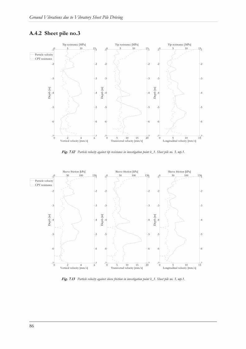
Ground Vibrations due to Vibratory Sheet Pile Driving
86
A.4.2 Sheet pile no.3
Fig. 7.12 Particle velocity against tip resistance in investigation point b_1. Sheet pile no. 3, mp.1.
Fig. 7.13 Particle velocity against sleeve friction in investigation point b_1. Sheet pile no. 3, mp.1.
0 2 4 6-7
-6
-5
-4
-3
-2
-1
Vertical velocity [mm/s]
Dep
th [m
]0 5 10 15
-7
-6
-5
-4
-3
-2
-1
Tip resistance [MPa]
0 5 10 15 20-7
-6
-5
-4
-3
-2
-1
Transversal velocity [mm/s]
Dep
th [m
]
0 5 10 15
-7
-6
-5
-4
-3
-2
-1
Tip resistance [MPa]
0 5 10 15-7
-6
-5
-4
-3
-2
-1
Longitudinal velocity [mm/s]
Dep
th [m
]
0 5 10 15
-7
-6
-5
-4
-3
-2
-1
Tip resistance [MPa]
Particle velocity
CPT resistance
0 2 4 6-7
-6
-5
-4
-3
-2
-1
Vertical velocity [mm/s]
Dep
th [m
]
0 50 100 150
-7
-6
-5
-4
-3
-2
-1
Sleeve friction [kPa]
0 5 10 15 20-7
-6
-5
-4
-3
-2
-1
Transversal velocity [mm/s]
Dep
th [m
]
0 50 100 150
-7
-6
-5
-4
-3
-2
-1
Sleeve friction [kPa]
0 5 10 15-7
-6
-5
-4
-3
-2
-1
Longitudinal velocity [mm/s]
Dep
th [m
]
0 50 100 150
-7
-6
-5
-4
-3
-2
-1
Sleeve friction [kPa]
Particle velocity
CPT resistance

Appendix
87
Fig. 7.14 Particle velocity against tip resistance in investigation point b_1. Sheet pile no. 3, mp.2.
Fig. 7.15 Particle velocity against sleeve friction in investigation point b_1. Sheet pile no. 3, mp.2.
0 2 4 6-7
-6
-5
-4
-3
-2
-1
Vertical velocity [mm/s]
Dep
th [m
]0 5 10 15
-7
-6
-5
-4
-3
-2
-1
Tip resistance [MPa]
0.5 1 1.5 2 2.5-7
-6
-5
-4
-3
-2
-1
Transversal velocity [mm/s]
Dep
th [m
]
0 5 10 15
-7
-6
-5
-4
-3
-2
-1
Tip resistance [MPa]
1 2 3 4-7
-6
-5
-4
-3
-2
-1
Longitudinal velocity [mm/s]
Dep
th [m
]
0 5 10 15
-7
-6
-5
-4
-3
-2
-1
Tip resistance [MPa]
Particle velocityCPT resistance
0 2 4 6-7
-6
-5
-4
-3
-2
-1
Vertical velocity [mm/s]
Dep
th [m
]
0 50 100 150
-7
-6
-5
-4
-3
-2
-1
Sleeve friction [kPa]
0.5 1 1.5 2 2.5-7
-6
-5
-4
-3
-2
-1
Transversal velocity [mm/s]
Dep
th [m
]
0 50 100 150
-7
-6
-5
-4
-3
-2
-1
Sleeve friction [kPa]
1 2 3 4-7
-6
-5
-4
-3
-2
-1
Longitudinal velocity [mm/s]
Dep
th [m
]
0 50 100 150
-7
-6
-5
-4
-3
-2
-1
Sleeve friction [kPa]
Particle velocityCPT resistance

Ground Vibrations due to Vibratory Sheet Pile Driving
88
Fig. 7.16 Particle velocity against tip resistance in investigation point b_5. Sheet pile no. 3, mp.1.
Fig. 7.17 Particle velocity against sleeve friction in investigation point b_5. Sheet pile no. 3, mp.1.
0 2 4 6-7
-6
-5
-4
-3
-2
-1
Vertical velocity [mm/s]
Dep
th [m
]0 2 4 6 8
-7
-6
-5
-4
-3
-2
-1
Tip resistance [MPa]
0 5 10 15 20-7
-6
-5
-4
-3
-2
-1
Transversal velocity [mm/s]
0 2 4 6 8
-7
-6
-5
-4
-3
-2
-1
Tip resistance [MPa]
0 5 10 15-7
-6
-5
-4
-3
-2
-1
Longitudinal velocity [mm/s]
0 2 4 6 8
-7
-6
-5
-4
-3
-2
-1
Tip resistance [MPa]
Particle velocity
CPT resistance
0 2 4 6-7
-6
-5
-4
-3
-2
-1
Vertical velocity [mm/s]
Dep
th [m
]
0 20 40 60
-7
-6
-5
-4
-3
-2
-1
Sleeve friction [kPa]
0 5 10 15 20-7
-6
-5
-4
-3
-2
-1
Transversal velocity [mm/s]
0 20 40 60
-7
-6
-5
-4
-3
-2
-1
Sleeve friction [kPa]
0 5 10 15-7
-6
-5
-4
-3
-2
-1
Longitudinal velocity [mm/s]
0 20 40 60
-7
-6
-5
-4
-3
-2
-1
Sleeve friction [kPa]
Particle velocityCPT resistance

Appendix
89
Fig. 7.18 Particle velocity against tip resistance in investigation point b_5. Sheet pile no. 3, mp.2.
Fig. 7.19 Particle velocity against sleeve friction in investigation point b_5. Sheet pile no. 3, mp.2.
0 2 4 6-7
-6
-5
-4
-3
-2
-1
Vertical velocity [mm/s]
Dep
th [m
]0 2 4 6 8
-7
-6
-5
-4
-3
-2
-1
Tip resistance [MPa]
0.5 1 1.5 2 2.5-7
-6
-5
-4
-3
-2
-1
Transversal velocity [mm/s]
0 2 4 6 8
-7
-6
-5
-4
-3
-2
-1
Tip resistance [MPa]
1 2 3 4-7
-6
-5
-4
-3
-2
-1
Longitudinal velocity [mm/s]
0 2 4 6 8
-7
-6
-5
-4
-3
-2
-1
Tip resistance [MPa]
Particle velocityCPT resistance
0 2 4 6-7
-6
-5
-4
-3
-2
-1
Vertical velocity [mm/s]
Dep
th [m
]
0 20 40 60
-7
-6
-5
-4
-3
-2
-1
Sleeve friction [kPa]
0.5 1 1.5 2 2.5-7
-6
-5
-4
-3
-2
-1
Transversal velocity [mm/s]
0 20 40 60
-7
-6
-5
-4
-3
-2
-1
Sleeve friction [kPa]
1 2 3 4-7
-6
-5
-4
-3
-2
-1
Longitudinal velocity [mm/s]
0 20 40 60
-7
-6
-5
-4
-3
-2
-1
Sleeve friction [kPa]
Particle velocityCPT resistance

Ground Vibrations due to Vibratory Sheet Pile Driving
90
A.5 Particle motion
A.5.1 Sheet pile no. 1
Fig. 7.20 Particle motion during 1 s, 10 s into the measurement of sheet pile no. 1, mp. 1.
-20 -10 0 10 20-20
-15
-10
-5
0
5
10
15
20
Transversal velocity [mm/s]
Ver
tical
vel
ocity
[mm
/s]
-20 -10 0 10 20-20
-15
-10
-5
0
5
10
15
20
Longitudinal velocity [mm/s]
Ver
tical
vel
ocity
[mm
/s]

Appendix
91
A.5.2 Sheet pile no. 2
Fig. 7.21 Particle motion during 1 s, 10 s into the measurement of sheet pile no. 2, mp. 1.
Fig. 7.22 Particle motion during 1 s, 10 s into the measurement of sheet pile no. 2, mp. 2.
Fig. 7.23 Three dimensional presentation of the particle motion for sheet pile no. 2. a) mp. 1 b) mp.2
-20 -10 0 10 20-20
-15
-10
-5
0
5
10
15
20
Transversal velocity [mm/s]
Ver
tical
vel
ocity
[mm
/s]
-20 -10 0 10 20-20
-15
-10
-5
0
5
10
15
20
Longitudinal velocity [mm/s]
Ver
tical
vel
ocity
[mm
/s]
-4 -2 0 2 4-4
-3
-2
-1
0
1
2
3
4
Transversal velocity [mm/s]
Ver
tical
vel
ocity
[mm
/s]
-4 -2 0 2 4-4
-3
-2
-1
0
1
2
3
4
Longitudinal velocity [mm/s]
Ver
tical
vel
ocity
[mm
/s]
-20-10
010
20
-20
-10
0
10
20-20
-10
0
10
20
TransversalLongitudinal
Ver
tical
-4-2
02
4
-4
-2
0
2
4-4
-2
0
2
4
TransversalLongitudinal
Ver
tical
b)a)

Ground Vibrations due to Vibratory Sheet Pile Driving
92
A.5.3 Sheet pile no. 3
Fig. 7.24 Particle motion during 1 s, 13 s into the measurement of sheet pile no. 3, mp. 1.
Fig. 7.25 Particle motion during 1 s, 13 s into the measurement of sheet pile no. 3, mp. 2.
Fig. 7.26 Three dimensional presentation of the particle motion for sheet pile no. 2. a) mp. 1 b) mp.2
-6 -4 -2 0 2 4 6-6
-4
-2
0
2
4
6
Transversal velocity [mm/s]
Ver
tical
vel
ocity
[mm
/s]
-6 -4 -2 0 2 4 6-6
-4
-2
0
2
4
6
Longitudinal velocity [mm/s]
Ver
tical
vel
ocity
[mm
/s]
-3 -2 -1 0 1 2 3-3
-2
-1
0
1
2
3
Transversal velocity [mm/s]
Ver
tical
vel
ocity
[mm
/s]
-3 -2 -1 0 1 2 3-3
-2
-1
0
1
2
3
Longitudinal velocity [mm/s]
Ver
tical
vel
ocity
[mm
/s]
-5
0
5
-5
0
5
-6
-4
-2
0
2
4
6
TransversalLongitudinal
Ver
tical
-2
0
2
-2
0
2
-3
-2
-1
0
1
2
3
TransversalLongitudinal
Ver
tical
a) b)
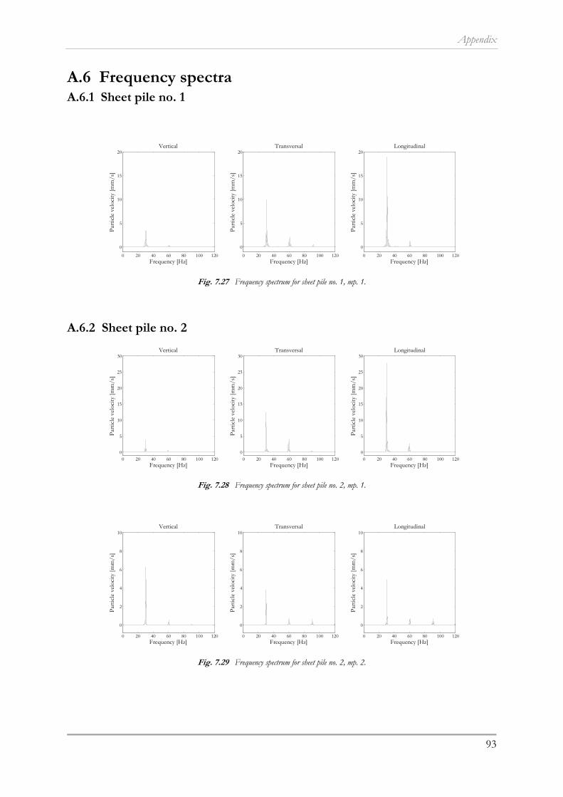
Appendix
93
A.6 Frequency spectra A.6.1 Sheet pile no. 1
Fig. 7.27 Frequency spectrum for sheet pile no. 1, mp. 1.
A.6.2 Sheet pile no. 2
Fig. 7.28 Frequency spectrum for sheet pile no. 2, mp. 1.
Fig. 7.29 Frequency spectrum for sheet pile no. 2, mp. 2.
0 20 40 60 80 100 120
0
5
10
15
20Vertical
Frequency [Hz]
Par
ticle
vel
ocity
[mm
/s]
0 20 40 60 80 100 120
0
5
10
15
20Transversal
Frequency [Hz]
Par
ticle
vel
ocity
[mm
/s]
0 20 40 60 80 100 120
0
5
10
15
20Longitudinal
Frequency [Hz]
Par
ticle
vel
ocity
[mm
/s]
0 20 40 60 80 100 1200
5
10
15
20
25
30Vertical
Frequency [Hz]
Par
ticle
vel
ocity
[mm
/s]
0 20 40 60 80 100 1200
5
10
15
20
25
30Transversal
Frequency [Hz]
Par
ticle
vel
ocity
[mm
/s]
0 20 40 60 80 100 1200
5
10
15
20
25
30Longitudinal
Frequency [Hz]
Par
ticle
vel
ocity
[mm
/s]
0 20 40 60 80 100 120
0
2
4
6
8
10Vertical
Frequency [Hz]
Par
ticle
vel
ocity
[mm
/s]
0 20 40 60 80 100 120
0
2
4
6
8
10Transversal
Frequency [Hz]
Par
ticle
vel
ocity
[mm
/s]
0 20 40 60 80 100 120
0
2
4
6
8
10Longitudinal
Frequency [Hz]
Par
ticle
vel
ocity
[mm
/s]

Ground Vibrations due to Vibratory Sheet Pile Driving
94
A.6.3 Sheet pile no. 3
Fig. 7.30 Frequency spectrum for sheet pile no. 3, mp. 1.
Fig. 7.31 Frequency spectrum for sheet pile no. 3, mp. 1.
0 20 40 60 80 100 120
0
2
4
6
8
10
12
14
16
18Vertical
Frequency [Hz]
Par
ticle
vel
ocity
[mm
/s]
0 20 40 60 80 100 120
0
2
4
6
8
10
12
14
16
18Transversal
Frequency [Hz]P
artic
le v
eloc
ity [m
m/s
]0 20 40 60 80 100 120
0
2
4
6
8
10
12
14
16
18Longitudinal
Frequency [Hz]
Par
ticle
vel
ocity
[mm
/s]
0 20 40 60 80 100 120
0
1
2
3
4
5
6
Vertical
Frequency [Hz]
Par
ticle
vel
ocity
[mm
/s]
0 20 40 60 80 100 120
0
1
2
3
4
5
6
Transversal
Frequency [Hz]
Par
ticle
vel
ocity
[mm
/s]
0 20 40 60 80 100 120
0
1
2
3
4
5
6
Longitudinal
Frequency [Hz]
Par
ticle
vel
ocity
[mm
/s]