grif 2011 petri nets with predicatesgrif-workshop.fr/download/doc/user manual-grif...
TRANSCRIPT

GRIF 2011
Petri Nets with predicates
User Manual
Version 31 January 2011
Copyright © 2011 Total

User Manual 2 / 76
Table of Contents1. Description of the interface ....................................................................................................... 4
1.1. Main window of the Petri Nets with predicates module .............................................................. 41.2. Description of the Menus ..................................................................................................... 41.3. Vertical Tool bar ................................................................................................................ 8
2. How to create a Petri Net ......................................................................................................... 92.1. Entering the Net ................................................................................................................. 9
2.1.1. Inputting Places ........................................................................................................... 92.1.2. Inputting Transitions ..................................................................................................... 92.1.3. Inputting Upstream and Downstream Arcs ...................................................................... 102.1.4. Inputting Local Data ................................................................................................... 112.1.5. Entering Comments ..................................................................................................... 12
2.2. Configuring the Elements ................................................................................................... 132.2.1. Configuring the Places ................................................................................................. 132.2.2. Configuring the Arcs ................................................................................................... 142.2.3. Configuring the Transitions .......................................................................................... 14
2.3. Data Editing Tables ........................................................................................................... 192.3.1. Description of the Tables ............................................................................................. 192.3.2. Arrangement of tables ................................................................................................. 212.3.3. Table Cleaning ........................................................................................................... 222.3.4. Data creation ............................................................................................................. 22
2.4. Arborescence .................................................................................................................... 232.5. Petri Net example ............................................................................................................. 242.6. Using repeated places (or shortcuts) ..................................................................................... 252.7. Page and group management ............................................................................................... 252.8. Data Entry Aids ................................................................................................................ 26
2.8.1. Copy / Paste / Renumber (without shortcut) ..................................................................... 272.8.2. Copy / Paste / Renumber (with shortcut) ......................................................................... 282.8.3. Copy / Paste / Renumber (with local data) ....................................................................... 282.8.4. Ordinary Copy/Paste ................................................................................................... 302.8.5. Overall change ........................................................................................................... 302.8.6. Selection change ......................................................................................................... 302.8.7. Document properties / Images management ..................................................................... 312.8.8. Alignment ................................................................................................................. 322.8.9. Multiple selection ....................................................................................................... 332.8.10. Selecting connex (adjacent) parts ................................................................................. 332.8.11. Page size ................................................................................................................. 332.8.12. Cross hair ................................................................................................................ 332.8.13. Gluing/Associating graphics ........................................................................................ 332.8.14. Prototypes ................................................................................................................ 34
3. Printing ................................................................................................................................. 35
4. Interactive simulation ............................................................................................................. 374.1. Transition firing ................................................................................................................ 374.2. Automatic firing of transitions with zero delay ....................................................................... 384.3. Probability firing for transitions with fire on demand ............................................................... 394.4. Simulation with groups present ............................................................................................ 394.5. Dynamic fields ................................................................................................................. 40
5. Statistics and Setup of Variables .............................................................................................. 425.1. Definition of statistic states ................................................................................................. 425.2. Configuration of statistic states (or variables) ......................................................................... 42
5.2.1. Types of statistics ....................................................................................................... 435.2.2. Computation times ...................................................................................................... 435.2.3. Histograms ................................................................................................................ 44
5.3. Tables and profil of variables .............................................................................................. 44

User Manual 3 / 76
6. MOCA computations .............................................................................................................. 466.1. Configuring the computations .............................................................................................. 466.2. Launching the computation (former GUI) .............................................................................. 47
6.2.1. Data tab .................................................................................................................... 476.2.2. Parameters tab ............................................................................................................ 506.2.3. Results tab ................................................................................................................. 51
6.3. Reading the results (former GUI) ......................................................................................... 526.4. Reading the results (New GUI) ............................................................................................ 55
6.4.1. Tables and Panels to display results ............................................................................... 556.4.2. Moca Results ............................................................................................................. 57
7. Curves .................................................................................................................................. 597.1. Charts Edit window ........................................................................................................... 597.2. Types of curves ................................................................................................................ 607.3. Examples of curves ........................................................................................................... 62
7.3.1. Moca 12 Curve .......................................................................................................... 627.3.2. Timing Chart ............................................................................................................. 637.3.3. Fixed Size Histogram .................................................................................................. 637.3.4. Equiprobable Classes Histogram .................................................................................... 647.3.5. Defined Interval Histogram .......................................................................................... 647.3.6. Curve from existing results ........................................................................................... 65
8. Databases .............................................................................................................................. 668.1. Connection to a CSV file ................................................................................................... 66
8.1.1. Form of the database ................................................................................................... 668.1.2. Connection ................................................................................................................ 66
8.2. Connection via a JDBC link (example with ODBC connector) ................................................... 678.2.1. Form of the database ................................................................................................... 678.2.2. Connection ................................................................................................................ 67
8.3. Operation ......................................................................................................................... 68
9. Save ...................................................................................................................................... 709.1. Model ............................................................................................................................. 709.2. RTF File .......................................................................................................................... 709.3. Input data ........................................................................................................................ 719.4. Results file ....................................................................................................................... 719.5. Curves ............................................................................................................................. 719.6. Tables ............................................................................................................................. 72
10. Options of GRIF - Petri Nets with predicates .......................................................................... 7310.1. Executables .................................................................................................................... 7310.2. Database ........................................................................................................................ 7310.3. Language ....................................................................................................................... 7310.4. Options .......................................................................................................................... 7310.5. Graphics ........................................................................................................................ 7410.6. Digital format ................................................................................................................. 7410.7. Places ............................................................................................................................ 7410.8. Transitions ..................................................................................................................... 7410.9. Arcs .............................................................................................................................. 7510.10. Local data .................................................................................................................... 7510.11. Simulation .................................................................................................................... 7510.12. Prototypes .................................................................................................................... 7510.13. Curves ......................................................................................................................... 75

User Manual 4 / 76
1. Description of the interface
1.1. Main window of the Petri Nets with predicates module
The main window is divided into several parts:
• Title bar: The title bar shows the names of the module and file being edited.
• Menu bar: The menu bar gives access to all the application's functions.
• Icon bar (shortcuts): The shortcut bar is an icon bar (horizontal) which gives faster access to the most commonfunctions.
• Tool bar: The tool bar (vertical) allows you to select the elements for modeling.
• Input zone: A maximum amount of space has been left for the graphical input zone for creating the model.
• Tree: A tree is "hiden" between input zone and tool bar. It enables to walk through pages and groups of thedocument.
• Set of tables: Tables are gathered in "hiden" tabs on the right.
1.2. Description of the Menus
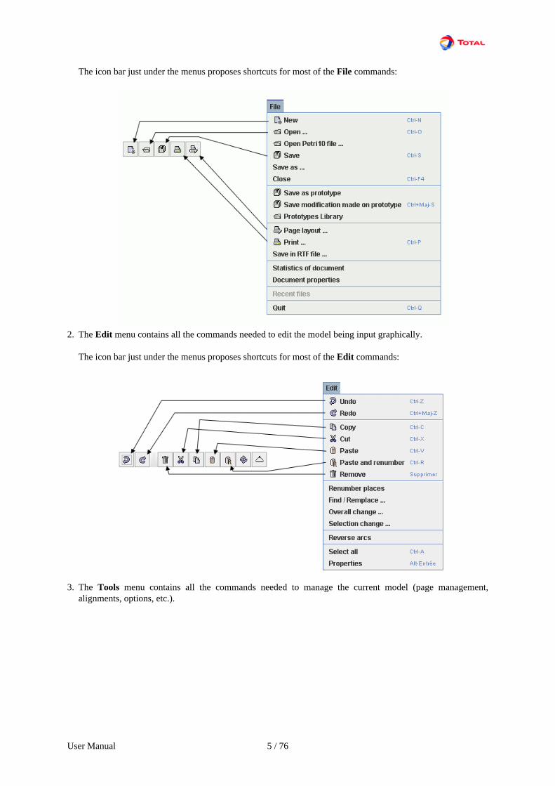
1. The File menu contains the standard commands used in this type of menu (open, close, save, print, etc.). Theproperties (name, creation date, created by, description, version) can be accessed and modified by selectingDocument properties. The Document statistics provide information on the model's complexity. It is alsopossible to access a certain number (configurable) of recently modified files.
User Manual 5 / 76
The icon bar just under the menus proposes shortcuts for most of the File commands:
2. The Edit menu contains all the commands needed to edit the model being input graphically.
The icon bar just under the menus proposes shortcuts for most of the Edit commands:
3. The Tools menu contains all the commands needed to manage the current model (page management,alignments, options, etc.).

User Manual 6 / 76
The icon bar just under the menus proposes shortcuts for most of the Tools commands:
4. The Document menu gives access to all the documents being created or modified.
5. The Petri Nets menu contains all the commands needed to produce the graphical part of the current model.
The vertical icon bar on the left of the application provides shortcuts for each of the Petri Nets commands(cf. vertical tool bar).

User Manual 7 / 76
6. The Data and Computations menu is divided into two parts: data management (creation and management ofthe different parameters) and configuration/computation launch (computation time, desired computation, etc.)..
Notes:
a. The Verify function detects any errors in the model: data without values (equal to NaN), places with anidentical number, etc.
b. The Export data function exports tables.
c. The Import data function imports tables.
7. The Mode menu switches from Input mode to Simulation mode.
8. The Group menu concerns the input and management of submodels grouped into independent subassemblies.
The icon bar just under the menus proposes shortcuts for two of the Group commands:
9. 9. Finally, the Help menu accesses the on-line Help, the Help topics and to "About".

User Manual 8 / 76
1.3. Vertical Tool bar
Each model used for operating safety has its own icons. All the Petri Nets graphical symbols are shown on thevertical icon bar on the left of the input window.
The vertical tool bar contains the following items:
• Places represented by circles.• Transitions represented by rectangles.• Upstream and downstream arcs represented by arrows.• Repeated place (Shortcut) to create links between several parts of the same model (on different pages or in
different groups).• Comment to add text directly on the chart.• Affichage dynamique to display the value of an element in the model.• Local data create variables linked only to one part of the model.• Charts to draw curves representing computations on the model.
• Simulation to switch to simulation mode.

User Manual 9 / 76
2. How to create a Petri Net
2.1. Entering the Net
2.1.1. Inputting Places
To input the different Places, select the corresponding symbol on the symbol bar. A new element is then createdeach time you click the mouse on the graphical input zone. Each of the places in the model has three parameters:
1. A number: Located in the centre of the places, they are automatically incremented. These numbers are the trueidentifiers of the places which will be used by the computation engine. This is why two places cannot havean identical number.
2. A label: A default label is assigned to each place ("Pli" for Place number "i"). Since each place normally hasa very precise meaning for the user you are strongly recommended to assign a label which is more mnemonicthan that given by default. This enables you to locate yourself better in the model and in the results file.
3. A number of tokens: By default it is equal to zero for each place created. In a Petri Net the presence (or not) ofa token in a place normally corresponds to the presence (or not) of a specific status for one of the componentsin the system modelled by the Petri Net. All the tokens present at a given instant (Petri Net "marking") thuscorrespond to the global status of the system studied. The change in this "marking" is the dynamic aspect ofthe system.
2.1.2. Inputting Transitions
To input the different Transitions, select the corresponding symbol on the symbol bar. A new element is thencreated each time you click the mouse in the graphical input zone.
In a Petri Net, the Transitions model the events which may happen at a given moment on the system studied(failures, tests, maintenance, etc.). Firing the transitions modifies the marking of the places to which they arelinked by the arcs (upstream and downstream). This is used to simulate the system's dynamic behaviour.
When created, each transition has a default name ("Tri" for the transition entered in the ith position). Unlike theplaces, the transition number is unimportant since it is not used in the data file generated for the computation

User Manual 10 / 76
engines. You are therefore highly recommended to assign them a mnemonic label (more than for the places) (cf.Section 2.2.3, “Configuring the Transitions”).
2.1.3. Inputting Upstream and Downstream Arcs
The "upstream arc" function describes part of the transition validation conditions (the other part is handled bythe "guards" - cf. Section 2.2.3.3, “Guards tab”). They define the marking necessary for the upstream places toallow the transition to be fired.
The "downstream arc" function describes what happens at token transfer level when the transition is fired.
To input the upstream or downstream arcs:
1. select one of the two corresponding icons on the symbol bar:
• the "single arrow" which is used to input only one arc at a time or
• the "double arrow" which is used to input as many arcs as you wish.
2. select a start Place (respectively a Transition) by clicking on it with the left mouse button
3. drag the mouse (without releasing the button) to the final Transition ( respectively the Place) and release thebutton.
It is the order "place" => "transition" or "transition" => "place" which determines the type ("upstream" or"downstream") of arc entered.
The result obtained is shown in the following figure. Upstream arcs have been drawn between place 1 and transitionTr1, then between place 2 and transition Tr2, and downstream arcs have been drawn between transition TR1 andplace 2, then between transition Tr2 and place 3, etc. It must be noted that, unlike the "Reliability Networks, thereare no bidirectional arcs for the "Petri Nets". However, it is often the case that a downstream arc must be drawn

User Manual 11 / 76
between the same place and the same transition. In this case they can be superimposed and give the illusion thatthey are a bidirectional arc but in fact they are two separate arcs.
Notes:
1. For reasons of model appearance or legibility it may be useful to break down an arc into several parts. To dothis, select the arc then move the small red square located in the middle of the segment.
2. It is also possible to straighten an arc using the command: Tools - Straighten arcs .
2.1.4. Inputting Local Data
To add local data to the model, select the corresponding icon on the task bar then click left at the point on themodel where the data is to be placed. A window then opens:
This dialogue box gives three choices:

User Manual 12 / 76
1. Create new data: opens a window where then you can create new data or a new parameter.
2. Use an existing variable: creates a graphical representation of a variable.
3. Use an existing parameter: creates a graphical representation of a parameter.
Once created, local data is represented as follows:
Click right on the local data to access its properties. Some fields can be modified in this manner: Name, domain,initial value, etc.
Note: the fields where the term "prototype" appears are only used to create a prototype (cf. appended documenton prototypes).
2.1.5. Entering Comments
To add a comment anywhere on the chart, click the pencil icon and place yourself on a point in the graphical inputzone. The Comment dialogue box opens where you can enter the desired comment.

User Manual 13 / 76
Note: Character "%" is a reserved character, it must be type twice "%%" in order to display "%".
2.2. Configuring the Elements
All the graphical elements can normally be edited with a double-click on them or using the Edit - Propertiesmenu, or using the shortcut Alt + Enter.
2.2.1. Configuring the Places
The various place parameters are entered as follows:
• Select the place using the right mouse button. A small panel then opens containing three fields to be filled in.
• Enter the place Name (optional but highly recommended). This description is "Pli" by default.
• Where necessary, change (carefully) the place Number. Other safer methods are described below.
• Enter the number of Tokens initially present in the place in question. This can be done manually but clickingthe small black triangle is much easier.

User Manual 14 / 76
Note : The Prototype part is only used to create prototypes (see prototypes appendix).
2.2.2. Configuring the Arcs
By default, the Weight of all the arcs (upstream and downstream) is "1". However, this can be modified. To dothis, click right on the arc relevant concerned to display the editor shown below.
Clicking the small black triangle displays some possible values which can be selected with the mouse. For thedownstream arcs, the weights are always positive and correspond to the number of tokens which will be added tothe downstream place when the corresponding transition is fired. For the upstream arcs there are three cases:
• Weight strictly positive: these are "normal" arcs which validate the transition when the number of tokens in theupstream place is greater than or equal to the weight of this arc. When the transition is fired, a number of tokensequal to the weight of the arc will be removed from the corresponding upstream place.
• Weight strictly negative: these are "inhibitor" arcs which inhibit the transition when the number of tokens in thecorresponding upstream place exceeds the absolute value of the arc weight (e.g. 3 tokens for a weight of -3).This type of arc is graphically represented by a dotted line and does not modify the marking of the upstreamplace when the transition is fired.
• Weight "0": it is an arc which empties the corresponding upstream place when the transition is fired (whateverthe marking of the upstream place before it is fired).
2.2.3. Configuring the Transitions
Entering the various transition parameters is more complex than those of places since it requires a goodunderstanding of the MOCA-RP application's possibilities. You are highly recommended to consult the manualat this stage of the operations!
Click right to select the transition concerned. A dialogue window appears. The top part allows you to modify theName and ID of the transition. The other part consists of 5 tabs for configuring the transition's behaviour.

User Manual 15 / 76
2.2.3.1. Delay tab
The Delay tab indicates the transition delay law. Select the desired law (see the MOCA-RP User's Manual), andthen enter the parameters of the law. In this example the default law is "Exponential" with 1E-3 as a parameter.For the parameters, you can enter a value, a name (a parameter) existing in the document, or a new name. In thislast case the following window will appear to ask for the value and the domain. In the example, Lambda is a RealParameter (invariable) with value 0.001.
It is also possible to use a Variable in the case of dynamic reliability.

User Manual 16 / 76
2.2.3.2. Fire tab
The Fire tab allows you to select the firing law for the transition:
• The Default law corresponds to the "normal" operation of the Petri Nets: the downstream places will be filledas defined in Section 2.2.2, “Configuring the Arcs”.
• The On demand fire law corresponds to the Moca-RP law of the same name: only one of the downstreamplaces is filled after firing. The arguments of this law are the (N-1)th probabilities of happening in one of the Ndownstream places. The last probability is computed by the computation engine by making the 1s complement(see "Moca-RP User's Manual" for more details).
• The On demand fire law corresponds to the Moca-RP law of the same name: only one of the downstreamplaces is filled after firing. The arguments of this law are the N-1 couple (probability,place). It is possible tospecify probability to go in a given place. There are N-1 couple because last couple is computed by making the1s complement, and using the place wich is not selected. (see "Moca-RP User's Manual" for more details).
• The Special laws can only be used in the very special case where the computation engine has been recompiledto take account of it (Cf. Moca-RP User's Manual).
2.2.3.3. Guards tab

User Manual 17 / 76
The Guard tab consists of a code editor where you can enter one (or more) guard(s) for the transition. A guard isa Boolean expression. The transition can only be fired if the guard is true.
The code editor has three parts. The first is an editable text zone where you enter the code using Moca-RP syntax.Under this zone is a noneditable zone indicating any errors which may arise. The third is the Tools part whichis a data entry aid.
The Syntax button makes a syntax change. The Semantics button checks the semantics. The errors are displayedin the bottom left part. Under the buttons there are drop-down menus giving access to the model's various data.Select the desired data then click the <= button to insert it in the code.
The Functions drop-down menu shows funtions that can be used in Moca (cf Moca User Manual).
2.2.3.4. Assignments tab
The Assignments tab contains a code editor (identical to that of the Guards tab) for entering the assignments. Theassignments are "played" when the transition is fired.
In Moca engine, usual behavior is the following: assignments are separate with "," and they are processed inparallel. You can ask for sequential processing of assignments using Sequential assignments check-box. In thiscase, each assignment must end with a ";".

User Manual 18 / 76
2.2.3.5. Others tab
The Others tab contains 4 options:
1. Selecting the Histogram check box tells MOCA-RP to record all this transition's firing instants and to printthem later.
2. The Transition with memory option: Once the transition has been configured you still have to specify whathappens when the transition is "inhibited" before it can effectively be "fired". This parameter is very importantand two very different cases must be considered:
• Case 1: When the transition is inhibited, this indicates that the corresponding event can never happen (e.g.:an "old" component is replaced by a "new" one before it fails ==> the old component can now never fail).In this case, when the transition becomes valid again, it represents a new event (e.g.: failure of the "new"component) which has nothing to do with that which was "nipped in the bud" before it could happen. Itis thus necessary to simulate a new firing delay for the transition: the transition has "no memory" of whathappened previously.
• Case 2: When the transition is inhibited, this only indicates that the corresponding event is temporarily"suspended" (e.g.: a component repair is stopped due to it being night time ==> the repair will continuewhere it left off the next morning). In this case, when the transition becomes valid again, this only meansthat the delay relative to the suspended event continues. We must therefore use the delay which remained atthe time when the transition was inhibited as the new delay before the transition is fired: the transition mustretain the "memory" of this residual delay. The choice is made by selecting (or not selecting) the Transitionwith memory check box.
You may need to erase memory, do to this you can input a condition to keep memory. If this condition (anexpression) get "false", the memory is "lost" and a new delay will be computed the next time the transitionbecomes valid.
3. The Priority check box is used to give the transition a priority level. If two transitions can be fired at a giveninstant, the one with the higher priority will be fired first. If the priority level is identical the transitions will befired in the chronological order of their creation. Since 2010 version, priority can be a complex expression.
4. The Prevent multiple triggers at the same time prevents from multiple Drc 0 or IFA/IPA firing without timeincrease.
5. The Equiprobable management of conflict provides an equiproble firing frequency of 2 or more transitionswhen they are in conflict.
6. The Private check box is only used to create prototypes (cf. prototypes appendix).
User Manual 19 / 76
2.2.3.6. Addition of guards
Once the transition's guards configured, it is possible to add one or more other guards. This functionality is availablein the transitions table (Edit transitions tab, located in the right side of the application). To add one or moreguards to one or more transitions, all we have to do is to select transition(s) to modify, then do a rigth click andfinally select the Add guard - With a "And" menu or the Add guard - With a "Or" menu. Add guard - With a"And" menu will add guard(s) to the selected transitions by doing a "logical And" with the existing guards. Addguard - With a "or" menu will add guard(s) to the selected transitions by doing a "logical Or" with the existingguards. Gaurds to add are entered thanks to a code editor.
2.2.3.7. Addition of assignments
Once the transition's assignments configured, it is possible to add one or more other assignments. This functionalityis available in the transitions table (Edit transitions tab, located in the right side of the application). To add oneor more assignments to one or more transitions, all we have to do is to select transition(s) to modify, then do arigth click and finally select the Add assignment menu. Assignments to add are entered thanks to a code editor.
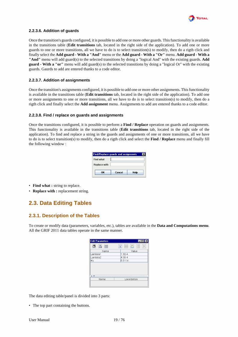
2.2.3.8. Find / replace on guards and assignments
Once the transitions configured, it is possible to perform a Find / Replace operation on guards and assignments.This functionality is available in the transitions table (Edit transitions tab, located in the right side of theapplication). To find and replace a string in the guards and assignments of one or more transitions, all we haveto do is to select transition(s) to modify, then do a rigth click and select the Find / Replace menu and finally fillthe following window :
• Find what : string to replace.• Replace with : replacement string.
2.3. Data Editing Tables
2.3.1. Description of the Tables
To create or modify data (parameters, variables, etc.), tables are available in the Data and Computations menu.All the GRIF 2011 data tables operate in the same manner.
The data editing table/panel is divided into 3 parts:
• The top part containing the buttons.

User Manual 20 / 76
• The main part containing the data table.• The bottom part indicating what the selected data is used for.
Saves the table in a text file.
Opens the table in a text editor (that defined in the Options).
Opens the column manager.
When the display selection button is pressed, a click in the table leads to the selection in the inputarea.
Displays the data filtering part.
Multiple modifications made to all the selected data.
Creates new data.
Deletes the selected data (one or many).
Enables data filtering or not.
Defines the filter to be applied to the data.
Filtering allows you to display only what is necessary in a table. Several filtering criteria can be combined, asshown below:
Select AND or OR to choose the type of association between each line (filter criterion). A line is a Booleanexpression divided into 3 parts:
1. the first is the column on which the filter is used;2. the second is the comparator;3. the third is the value to which the data will be compared.
If the Boolean expression is true, the data will be kept (displayed); otherwise the data will be masked. When thefilter is enabled its value is displayed between < and >.
The data in a column can be sorted by double clicking the header of this column. The first double click will sortthe data in ascending order (small triangle pointing upwards). The second double click on the same header willsort the column in descending order (small triangle pointing downwards).
A table can contain many columns, some columns may be unnecessary in certain cases. The "linked to database"column is unnecessary when no database is available. It is thus possible to choose the columns to be displayedand their order. To do this, click right on a table header, or click the Columns Manager button, the followingwindow opens:

User Manual 21 / 76
You can choose the columns to be displayed by selecting (or deselecting) the corresponding check boxes. Thearrows on the right are used to move the columns up or down in the list to choose the order of the columns. TheDisable data sorting check box disables the data sorting. This improves the application's performance with verycomplex models.
To modify data, double click the box to be modified. When several lines are selected (using the CTRL or SHIFTkeys) changes can be made to all the selected data by using Multiple changes. A window then opens to allowyou to make these changes.
Items which cannot be modified are greyed. The white lines indicate that the selected data does not have the samevalue for the field in question. A new value can be entered which will be taken into account for all the selecteddata. The lines with no background colour indicate that all the selected data has the same value for this field (inthis example the selected data is all "Float"); they can be changed to give a new value to all the selected data.
The bottom table in the data table indicates which elements in the model use the selected data. The first columnof this table gives the name of these elements; the second indicates their location in the document (page, group).Clicking on a line in this bottom table opens the page where the element is located and selects the element.
2.3.2. Arrangement of tables
As said before, tables are available in Data and Computations menu, In this case, each table is openned in aseparate window.
To decrease number of openned windows, tables are gathered in a tabbed pane at the right of the application. Thepane can be "hiden" with the little arrows at the top of split-pane.
User Manual 22 / 76
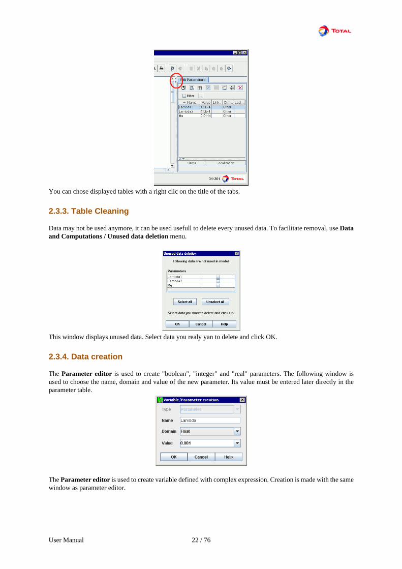
You can chose displayed tables with a right clic on the title of the tabs.
2.3.3. Table Cleaning
Data may not be used anymore, it can be used usefull to delete every unused data. To facilitate removal, use Dataand Computations / Unused data deletion menu.
This window displays unused data. Select data you realy yan to delete and click OK.
2.3.4. Data creation
The Parameter editor is used to create "boolean", "integer" and "real" parameters. The following window isused to choose the name, domain and value of the new parameter. Its value must be entered later directly in theparameter table.
The Parameter editor is used to create variable defined with complex expression. Creation is made with the samewindow as parameter editor.

User Manual 23 / 76
When variable is created, a double click in definition part opens code editor.
The code editor has three parts. The first is an editable text zone where you enter the code using Moca-RP syntax.Under this zone is a noneditable zone indicating any errors which may arise. The third is the Tools part whichis a data entry aid.
The Syntax button makes a syntax change. The Semantics button checks the semantics. The errors are displayedin the bottom left part. Under the buttons there are drop-down menus giving access to the model's various data.Select the desired data then click the <= button to insert it in the code.
The Functions drop-down menu shows funtions that can be used in Moca (cf Moca User Manual).The third menu display function that are available in MocaAdd.dll, for more information (cf Moca12 user manual)
A parameter can be transformed into variable and vice versa, by right-clincking on it and selectiong Change tovariable ou Change to paramètre
2.4. Arborescence
To help users to walk through the document (pages, groups ans sub-groups), a tree is available of the leaf of theapplication. By default, every element is displayed, you can use Filter button in order to select elements you wantto display or not.
You can expand or collapse a node in a recursive way with a right click on the node.
As explained for tables on the right, you can "hide" the tree.

User Manual 24 / 76
2.5. Petri Net example
The small Petri Net above represents the behaviour of a piece of equipment repaired by a maintenance team whichis not necessarily available when the equipment fails.
This net has three places:
• Work: operating (place 1)• Failed: failed, awaiting repair ( place 2)• Repair: being repaired (place3)
And three transitions:
• Failure: failure of the equipment• Repair_Start: the equipment will be repaired• Repair_End : the equipment is repaired and restarts
Here is how the model can be used to simulate the behaviour of a real piece of equipment
1. The Work place initially contains a token and the result is that the Failure transition is the only transition validat the initial instant.
2. It will be fired when the component fails (delay fired randomly according to the exponential law assigned tothis transition). The effect of this will be to remove the token from the Work place and to place one in theFailed place. In addition the Production variable will be reset to 0.
3. Since the arrival of the token in the Failed place is not sufficient to validate the Repair_Start transition, wemust wait until the RepairTeam_OK variable (the message) input (or guard) to this transition becomes TRUE.
4. When the team of repairers is available (RepairTeam_OK message changes to TRUE) then the repair willimmediately start since the delay law for this transition is a Dirac law with a zero delay.
5. When the Repair_Start transition is fired, the token is removed from the Failed place, a token is placed inthe Repair place and the RepairTeam_OK message changes to FALSE (meaning "Repairers Unavailable").Therefore, if another piece of equipment fails it must wait until the team of repairers is free before it can berepaired.
6. The arrival of the token in the Repair place validates the Repair_End transition which will be fired at the endof the repair delay (delay fired randomly according to the exponential law assigned to this transition).
7. When the Repair_End transition is fired, this removes the token from the Repair place, places a token inthe Work place and again changes the RepairTeam_OK message to TRUE. The Production variable takes

User Manual 25 / 76
the ProdMAX value (100). Therefore we have returned to the initial state and the equipment is ready for thesimulation of its second failure, etc.
We have taken exponential laws but any other type of laws could have been used (e.g.: the log-normal law forthe duration of the repair). Also, the Dirac law has enabled us to mix a deterministic phenomenon with randomphenomena without hesitation. Therefore, although it is very simple, this small model already gives an idea of thepower of the Petri Nets associated with the Monte Carlo simulation.
2.6. Using repeated places (or shortcuts)
The concept of a shortcut (or repeated element) was introduced in the Petri Nets with predicates module for fourmain reasons:
• To link together portions of the model;• To avoid graphicaly complex model, and keep readability;• To simplify the use of the Group function (cf. below);• To highlight what is essential and what is not.
In order to create a repeated place, select the repeated place icon in the toolbar, then click on place (here placenumber 4). The repeated place (or shortcut) is displayed as a number if place has no token, or as a coloredrectangle if place contains tokens.
Then, the repeated place can be selected to be put where tou want. You link the shorcut to a transition with an arc.Operation can be repeated many times (2 times on figure).
The behavior of this Petri Net is the same as the one describe in above paragraph. Messages have been replacedby Repair_Team place. For the net describing equipment behavior, the Repair_Team place is auxiliary.
2.7. Page and group management
The use of shortcuts allowed us to obtain two Petri Nets which have no graphical link between them. Theycommunicate only by shortcuts. This can be used, for example, to place each subpart on a different page:

User Manual 26 / 76
1. Create a new page by clicking the corresponding icon in the icon bar (or use menu Tools - New Page). A pagenumber 2 is thus created.
2. Return to page 1 by selecting the page using the page selector in the ideographic command bar (or use menuTools - Page manager).
3. Select the part to be moved.4. Open menu Tools - Change page.5. Select page 2 and click OK. The part selected is transferred to page 2 but it continues to communicate with
page 1 via the shortcuts.
Note: For large models the division method described above is very useful.
Another possibility for entering large Petri Nets is to use the Group concept. This is made possible by the shortcutsand the fact that the data is global for a document. This allows quite separate subparts to be created:
1. Select a subpart.2. Use menu Group - Group. A dialogue box then opens asking for the name to be given to the group being
created.3. Enter the desired name and click OK (e.g.: "System 1"). The group is created: the subnet is replaced by a
rectangle assigned with the chosen name.
You can also create an empty group with Group - New Group menu or group tool in the left toolbar.
Each group can then be edited, renamed or ungrouped using the commands in the Group menu. The group canalso be edited with a click right or using the "cursor down arrow" on the left of the page manager. In Edit mode,the submodel can then be modified as you wish. When the modification is terminated you return to the previousfigure by exiting group editing by menu Group - Quit Group Edition, or using the "cursor up arrow" on the leftof the page manager. It's also possible to choose a picture for a group by using Group - Change Picture menu.
Note: Groups can be grouped recursively.
2.8. Data Entry Aids
To simplify model creation the Petri Nets with predicates module has different data entry aids to automate time-consuming operations.

User Manual 27 / 76
2.8.1. Copy / Paste / Renumber (without shortcut)
To assist with the entry of the repeated parts of the Petri Nets "Copy / Paste and Renumber" mechanisms havebeen provided. This operation is carried out in 6 steps:
1. Select the part to be copied.2. Click the Copy icon, or use menu Edit - Copy or the shortcut Ctrl + C.3. Click the Paste and Renumber icon, or use menu Edit - Paste and Renumber or the shortcut Ctrl + R.4. A window appears where you choose the start number for the renumbering.5. The previously selected part is copied and the copy is selected.6. Move the copy to the desired location.
We then obtain the net shown in the figure opposite/ below: Places 1, 2 and 3 of the original have been transformedinto 4, 5 and 6 for the copy.
When copying to a new document, any data conflicts are handled in the following window:
This window shows all the data which has the same name in the source document and the destination document.There are three choices:
1. Use data of destination document, this will replace the occurrences of the data in the source document by thedata with the same name in the destination document.
2. Create a copy for each data in conflict, this will replace the occurrences of the data in the source document bya copy with a name with the suffix "copy".

User Manual 28 / 76
3. Manually manage conflict, this allows you to choose whether you use the existing data or not, depending on thedata. You can also specify the name of the copy by double clicking on the box in the "destination document"column. The names in this column are normally masked when the Use existing check box is selected, since itis the data which is already in the destination document which will be used.
2.8.2. Copy / Paste / Renumber (with shortcut)
The "Copy / Paste and Renumber" command creates new "instances" i.e. new subcharts similar to the subchartcopied:
• Same graphical structure;
• Same probability law;
• Same guards and assignments;
• Same labels but different places and transitions from those copied.
When creating a new instance it is therefore necessary to make the distinction between the places repeated"internally" (specifically belonging to the subchart copied) and the places repeated "externally" (attached to aplace not belonging to the subchart copied). Only the places repeated "internally" must be renumbered. The placesrepeated "externally" must normally not change numbers.
Remarque: Only the "shortcuts" of the places present in the selection to be renumbered (differentiated from theothers by a double circle) are actually renumbered. Therefore the corresponding "input" shortcuts (represented bysmall rectangles) are renumbered in their turn. The result is that the "shortcuts" on the places not belonging tothe selection are not renumbered.
The above figure explicitly illustrated the mechanism. Repeated place number 1 (internal to the original subchart)has been renumbered as 5 on the copy. However, the numbering of the corresponding shortcuts to place 4 (externalto the copy) has not changed.
You can navigate between an element's different shortcuts, using menu Tools/Navigate to shortcuts. A windowopens and displays the list of shortcuts. Clicking on a shortcut automatically positions the view on this shortcut.You can return to the original element by clicking on its name at the top of the window.
2.8.3. Copy / Paste / Renumber (with local data)
When you wish to perform a "Copy / Paste and Renumber" operation by including local data in the copy, a dialoguebox will open during the "Paste" step. This window allows you to rename the copy of the local data.

User Manual 29 / 76
The above figure shows that the name assigned by default to the copy of the local data is "original name" + "Copy".This name, which is not necessarily well-adapted, can be modified.
Once the copy is made, new local data is created. Where necessary, if the definition of the original local data islinked to the associated net (included in the copy), then the definition of the local data copy the will remain thesame with respect to the net copy.
The above figure clearly shows that new local data has been created. It is called Dispo_B. Dispo_A is equal to thenumber of tokens present in place no. 1, Dispo_B is equal to the number of tokens in place no. 4.
Note: The main advantage of the local data is that of being able to perform "Copy / Paste and Renumber" operationssuch as those described above.

User Manual 30 / 76
2.8.4. Ordinary Copy/Paste
In addition to the "Copy / Paste and Renumber" command there is an ordinary "Copy / Paste" function. It is usedto make a single copy without renumbering. We thus obtain double elements which, from a formal viewpoint, isincorrect but which must be temporarily tolerated to simplify data entry.
Where possible, the "Copy / Paste and Renumber" function must be used in preference to the simple "Copy / Paste"function to minimise the risk of errors. But when it is used you must take the necessary precautions to re-establishthe correct numbering to eliminate the duplicates.
2.8.5. Overall change
When creating the Petri Nets it may be necessary to change a large part of the elements in the models: changingthe names, numbers, etc. The "Replace all" function in the Edit menu allows you to perform overall changes:
• Use the Edit / Overall changes function.
• Choose the type of elements to be modified among available tabs.
• The "Find / Replace" part changes a character string present in one or more variable labels, place labels ortransition labels. It is replaced by the string entered in the "Replace" part.
• The "Renumber" part only concerns the places. It is used to change place numbers. You indicate a Start numberthen specify a constant Step, or Add a constant value to the current numbers.
• Click OK to return to the chart. The changes are validated.
Note: The name changes and renumbering can be done manually if the necessary precautions are taken (avoidingduplicates, etc.). You click the Future number or Future name column and enter the change. Do not forget tovalidate it with the "ENTER" key.
2.8.6. Selection change
The "Selection change" function is equivalent to a "Replace all" but only applied to the selected elements. Theonly difference is that we must make the distinction between "internal" and "external" variables/parameters.
• "Internal" variable/parameter: only used within the selection
• "External" variable/parameter: used within the selection but also used elsewhere in the model.
Only the "internal" elements can change their name. If a variable or a parameter is recognised as being "external",the check box in the Internal column must be selected before it can be modified. The change will only affect theselected part. Everything outside the selection will remain unchanged.

User Manual 31 / 76
In the above example only the name of parameter "Lambda2" will change (in the "Replace selection" sense) sinceit is "internal" to the selection. A new parameter called "Def2" (with identical value) will be created and willreplace "Lambda2" in the model. The other parameter, which is not "internal", will remain unchanged.
2.8.7. Document properties / Images management
File - Doucument properties menu enable to save information about document : name, version, comment, ...These informations are available in General tab.
Images may be very useful to represent sub-system. GRIF 2011 enables to save images that can be used in differentparts of software (groupes, prototypes, ...). Images management is made in Images tab.

User Manual 32 / 76
To add a new picture into document, use icon. A double click in File column enables to select an picture (jpg,gif or png). A double click in Description column enables to give a name or a description to selected image.
Once in document, picture can be linked to a groupe with Group - Picture change menu.
Images are saved indide document, pay attention to picture size. Because images are inside document, you haveto re-add picture if picture is modified erternaly.
2.8.8. Alignment
To improve the legibility of the model the selected elements can be aligned vertically or horizontally. To do this,use the Align command in the Tools menu.
The following figure shows how the command works. For example, to align selected places and transitionsvertically, proceed as follows:
1. Select the elements (places, transitions, comments, etc.) to be aligned;
2. Go into the Tools menu and select the Align function;
3. Choose the type of alignment: Align center;
4. Click left on the mouse.

User Manual 33 / 76
Similarly, to align elements horizontally select the type Align middle which aligns the ordinates while keepingthe abscissa constant. The principle is the same as that described above.
2.8.9. Multiple selection
It may sometimes be useful to select several elements located in the four corners of the input zone. To simplifythis type of selection click on each of the desired elements one by one while holding down the Shift key on thekeyboard.
2.8.10. Selecting connex (adjacent) parts
It is sometimes difficult to select an additional part of a model. To simplify the selection process, select a graphicalelement then use menu Select connex part in the Edit menu. The additional part can be selected directly byclicking on the element while keeping the Control button pressed.
2.8.11. Page size
If, during modeling, the page size is insufficient it can be changed using menus Increase page size, Reduce pagesize or Page size in the Tools menu.
2.8.12. Cross hair
To be able to create an ordered and legible model quickly, the cross hair can be used to align the different elementswith each other (but less accurately than the Align function in the Tools menu). The cross hair is enabled (ordisabled) in the Graphics tab of the Option menu.
The following picture show how to quickly align two element of the model.
In order to align horizontally, select Align au middle which align keeping constant abscissa.
2.8.13. Gluing/Associating graphics
When objects are where you want, you can glue a set of object by right-clicking and selecting Glue. This commandcreate a group (a graphical one, not a hierarchical one) with selected objects, so that moving one moves the others.

User Manual 34 / 76
2.8.14. Prototypes
cf. appendix about prototypes
User Manual 35 / 76
3. Printing
For printing, you have several commands at your disposal in the File menu File:
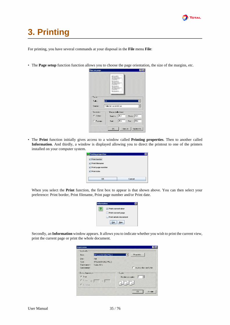
• The Page setup function function allows you to choose the page orientation, the size of the margins, etc.
• The Print function initially gives access to a window called Printing properties. Then to another calledInformation. And thirdly, a window is displayed allowing you to direct the printout to one of the printersinstalled on your computer system.
When you select the Print function, the first box to appear is that shown above. You can then select yourpreference: Print border, Print filename, Print page number and/or Print date.
Secondly, an Information window appears. It allows you to indicate whether you wish to print the current view,print the current page or print the whole document.

User Manual 36 / 76
The Print window will not be described here since it depends on your system.
• It is also possible to select the Save to RTF file function. Two windows are then displayed consecutively toyou, called Print properties and Information (identical to those of the Print function). You are then asked tochoose the folder in which the RTF file is to be saved.

User Manual 37 / 76
4. Interactive simulation
4.1. Transition firing
One of the most important features of the GRIF interface is that it can be used to manually simulate the behaviourof the net which has just been input. It is therefore easier to understand, debug or explain a model. To enable thisfunction, click the corresponding icon in the tool bar or use menu Mode - Simulation.
When simulation mode has been enabled, all the "valid" transitions immediately appear in red in the initial stateof the Petri Nets.
In the above figure, two transitions are valid in the initial state. They respectively correspond to the failure of theequipment on the right and to the failure of the equipment on the left. The two transitions called Failure are validsince there is a token in each of their respective upstream places (Work).
This simulation is that expected: at the initial instant (when the system is perfect), the only thing which can happenis that one of the two components might fail.
The operation which is of major interest is to be able to "manually fire" the valid transitions:
• choose one of the valid transitions;
• click left on this transition.
The result of this is to:
• remove the token from the Work place (which inhibits the Failure transition);
• add a token in the Failed place.

User Manual 38 / 76
In the example, given that the Boolean variable RepairTeam_OK is initially TRUE, the Repair_Start transitionof the component which failed (that on the left) will be valid. As for the other component, its Failure transitionwill remain valid.
4.2. Automatic firing of transitions with zero delay
The automatic firing of the transitions in simulation mode automatically fires the transitions which have a zerodelay (Dirac law with parameter 0) when they are valid. In the case where several Dirac law transitions are in"conflict", the transitions are fired according to their priority, then in chronological order of their creation on apage, then in increasing order of pages. This is how the simulation works when the computations are launched.
Remarque: The transitions with zero delay of a group are fired after those of the page where this same group figures.

User Manual 39 / 76
To enable or disable this function go into Application Option - Simulation:
4.3. Probability firing for transitions with fire on demand
In simulation mode, when we wish to fire a transition with "fire on demand", the token(s) must only move to asingle place downstream. When you click on this type of transition a window is displayed where you have to enterthe probability manually (it is normally a probability which is determined by a simulation).
Note: The default value of this probability is 0.5.
In the above example, if 0.5 is entered, the token will go into place no. 3.
4.4. Simulation with groups present
To fire one or more valid transitions which are contained in a group there are two ways of proceeding:
• enter the group and fire the transitions by clicking directly on them (click left on the group or click right thenselect Edit group);

User Manual 40 / 76
• or fire the transition simply using the list of valid transitions contained in the group and the "subgroups" (clickright on the group).
Again in the previous example, with the two components, the Failure transition was the only valid transition.
When transition are fired inside groups, it's difficult to see what appens. That why dynamic fields are useful.
4.5. Dynamic fields
It may be useful to observe the change in the different parameters of the model. To do this, use dynamic fields byselecting the corresponding icon on the vertical tool bar:
The dynamic fields are a type of "improved comments". They can be used not only to enter words or phrases butalso to insert model values.
• la date;
• value of a variable (you select the variable from a drop-down list);
• value of a parameter (you select the parameter from a drop-down list);
• number of tokens in a place (you must enter the number of the target place);
• expression of a variable (you select the variable from a drop-down list).
When you have made your choice from the five types of elements which it is possible to observe, a piece of codeis inserted in the text part. This will give access to the parameter value. If the dynamic field inserted does notcorrespond to any of the model's elements (variable which no longer exists, place number not assigned, etc.) thenthe inscription undef is displayed.
Note: To differentiate them, the dynamic fields are displayed in red (unlike the comments which are displayedin blue).
Note2: Character "%" is a reserved character, it must be type twice "%%" in order to display "%".

User Manual 41 / 76
Example of a dynamic field allowing the value of a parameter X to be observed:

User Manual 42 / 76
5. Statistics and Setup of Variables
In addition to the mean marking of the places and of the mean number of times each transition is fired, thesimulation can compute a certain number of additional statistics. Statistical results can be obtained on any of themodel's variables or combination of variables. To do this, a variable must be declared as "observed". When avariable is "observed", a statistic state (Moca meaning) is created for computation.
5.1. Definition of statistic states
A statistic state is defined like an "Observed" variable. We must initially define the statistic states we wish toobserve. To do this, we have to edit variables from the model : either thanks to the Data and computations - EditVariables menu, or thanks to the Edit Variables tab. Then, all we have to do is to set Observed property of avariable in order to make it a statistic state.
5.2. Configuration of statistic states (or variables)
Once variable is observed, we have to configure them by specifying types of computations and computation timesto be carried out on them, ... To do this, we have do a right-clic on the variable and select Configuration ofcomputation.

User Manual 43 / 76
The window to edit observed variables (statistic states) is made of two tabs. The first tab is for computation, thesecond one is for histograms. These two tabs enables configuration of Types of statistics, Computation timesand Histograms.
5.2.1. Types of statistics
Types of statistical computations are the following :
• 1 - Cumulated time where value is not null : This is the mean time in which the statistic state is differentto 0 on a history.
Purpose: Mainly used to compute mean availabilities during a history.
• 2 - Probability to have a not null value at t : This is the probability that the statistic state is different to zeroat the end of the history.
Purpose: Among other things, used to compute the mean availability at the end of a history or compute thereliability (to find if the failure state - which is an absorbent state - is present at the end of a history).
• 3 - Value at t : This is the mean value of the statistic state at the end of the history.
Purpose: This type of computation can be used to compute the occurrence of specific event during a history.
• 4 - Number of changes from null value to not null value between 0 and t : This is the mean number of timesduring a history that the statistic state changes from a zero value to a non-zero value.
Purpose: This type of computation can be used to compute the occurrence of specific events during a history.
• 5- Mean value from 0 to t : This is the mean value of the statistic state on the duration of the history.
Purpose: Among other things, used to compute the production availability.
• Date of first affectation to a not null value : This is the mean instant from which the value of the statisticstate changes from zero to a value different to zero.
Note: The "uncensored data" field gives the number of histories for which the simulation has been able toretrieve a value. For this mean statistical result to have a meaning, we must verify that a value has been retrievedfor each history (uncensored data = number of simulated histories).
Purpose: Used to obtain information about the mean instant when a system fails for the first time (reliabilitycomputations, estimation of the mean trouble-free operating time, etc.).
5.2.2. Computation times
Two possibilities are available to define computation times :
• List of times : the computations will be performed for the values of t given in this list. Separator is comma.
• Iterate Form A to B step C : the computations will be performed for values of t ranging from A to B with astep of C. You can also choose is computations are made before or after transitions triggering.

User Manual 44 / 76
5.2.3. Histograms
Computations made previously gives mean value for many histories. Histograms enable to know how values aredistributed during histories. (Cf. Moca User manuel for further information)
• List of values : provides value at the end of each history.• Fixed size intervals : provides the way value are distributed by cutting intervals of values in X intervals which
size is equal.• Equiprobable classe intervals : provides intervals whose probability to contains a value at the end of a story
id the same.• User-defined Intervals
Bounds of intervals can be defined as follows :• Automaticaly defined limits for SIL• Manual definition of limits (separate by commas)• "Iteration" : user choose lower limit and upper limit, and the size of intervals.• "Iteration (log scale)" : user choose lower limit and upper limit, and the number of intervals. Size of intervals
will be computed in order to have same-size-intervals, on a logarithmic scale.
Moreover, two limits are added at minus infinity, and plus infinity, in order to have a chart containing everyhistory of the simulation.
When limits are chosen, user has to choose between "left inclued" or "right included". Nb : IEC 61508 specifies"left included" intervals for SIL
5.3. Tables and profil of variables
You can create data-tables (or global-tables) with Tables table. A global-table is a list of arguments which canbe used in functions needing several arguments.
User Manual 45 / 76
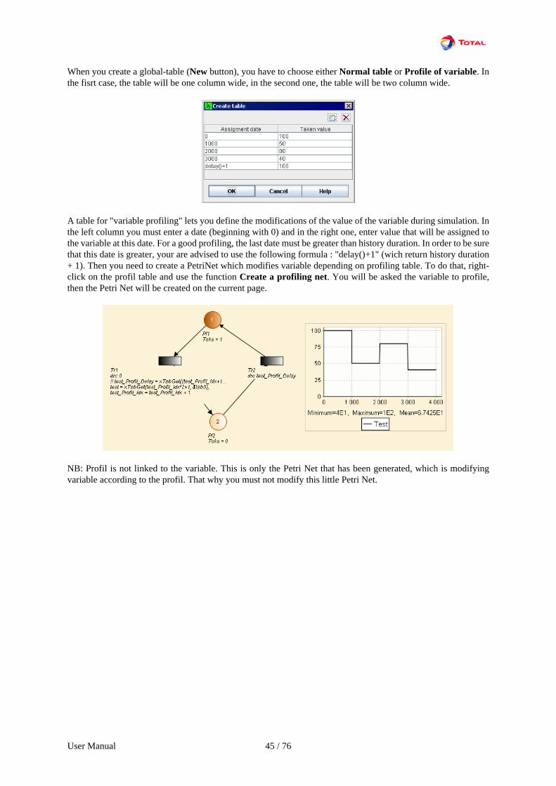
When you create a global-table (New button), you have to choose either Normal table or Profile of variable. Inthe fisrt case, the table will be one column wide, in the second one, the table will be two column wide.
A table for "variable profiling" lets you define the modifications of the value of the variable during simulation. Inthe left column you must enter a date (beginning with 0) and in the right one, enter value that will be assigned tothe variable at this date. For a good profiling, the last date must be greater than history duration. In order to be surethat this date is greater, your are advised to use the following formula : "delay()+1" (wich return history duration+ 1). Then you need to create a PetriNet which modifies variable depending on profiling table. To do that, right-click on the profil table and use the function Create a profiling net. You will be asked the variable to profile,then the Petri Net will be created on the current page.
NB: Profil is not linked to the variable. This is only the Petri Net that has been generated, which is modifyingvariable according to the profil. That why you must not modify this little Petri Net.

User Manual 46 / 76
6. MOCA computations
The computations using MOCA-RP V12 are performed in three main steps:
• general configuration of parameters;• the launch itself;• reading the results file.
6.1. Configuring the computations
The computation configuration window can be accessed in two different ways: either via menu Data andComputations - Moca Data or via Data and Computations - Launch Moca 12 .... The difference between thetwo is that, in the second case, the configuration step is directly followed by the computation launch step.
The configuration window which opens is called General Information:
This configuration window is divided into five parts:
1. Title: allows you to give a title to the results file.
2. Default statistics configuration: defines the types of computations which will be performed by default forall the statistic states.
3. Default computation times for statistic states:
• Iterate From A to B step C: the computations will be performed for values of t ranging from A to B witha step of C.
• List of times: the computations will be performed for the values of t given in this list.

User Manual 47 / 76
<listitem>Computation made at: by default, computations are made immediatly after trantion triggering, but you cando computation et t-Epsilon (just before triggering), or at both.</listitem>
4. General:
• Number of histories: Number of histories (NH) to be simulated (each history has a time t indicated below).
• First random number: It is the seed of random number generator.
• Maximum computation time (MT): The computations are stopped and the results are printed even if therequested number of histories has not been reached.
Note: the unit of time (MT) is the second.
• Automatic history duration: If this box is checked, GRIF will compute history duration using computationtime of variables and statistical states. If not, user can choose a specific History duration
• Multi-processors computing Enables (or not) the multi-processor computing (when available).
• Activate uncertainty propagation Enables (or not) the uncertainty propagation computations (two-stagesimulation): in this case we must specify the number of sets of parameters "played" (the real number ofhistories thus simulated will be the "number of sets of parameters x number of histories to be simulated" andwill be displayed in the "Total number of histories" field).
5. Variables: This tabs reminds comuting configuration of variables. If document contains some statistical states,another tab is available.
6. Output: used to configure the output.
• Prints the description of the Petri Net in the results file (or not)
• Prints the results file allowing it to be loaded using a spreadsheet application (such as EXCEL)
• Prints the censored delays (or not)
• Number of outputs during simulation. If 2 outputs, there will be an output at NH/2 and at NH.
7. Advanced options: used to configure the advanced options.
• You can choose the limit of transitions fired at the same time before loop detection.
6.2. Launching the computation (former GUI)
When the configuration part has been carefully carried out, a window is displayed where you launch thecomputations. This window has three tabs: Data, Parameters and Results.
6.2.1. Data tab
The Data tab displays the MOCA-RP V12 input data file (file type: ".don"). In addition to being able to modifythis file manually, there are four buttons available allowing you to perform the following operations:
• Open: opens a data file;
• Save: saves the current file;
• Clear: clears the content of the current file;

User Manual 48 / 76
• Generate data: generates input data from document.
An input data file is generally a long file with the following main parts (from top to bottom):
1. General information: it is simply the description of the parameters defined in the General Information window(cf. above)
2. Declaration of the net variables and parameters
3. Description of the net: the transitions are described one after another in the order in which they were generatedby GRIF.

User Manual 49 / 76
Example of a description of a transition:
This is how the description of a transition must be read.
• "TR": keyword indicating that a new transition will be described
• "AM" and "AV": keywords respectively indicating the description of the upstream and downstream arcs(place no. and weight of the corresponding arc)
• "??": indicates the description of the transition guards
• "!!": indicates the description of the transition assignments
• "LOI": keyword indicating the start of the description of the law governing the transition delay computation
• "TIR": keyword indicating the start of the description of the law governing the type of the transition firing
4. Mnemonic of the places
5. Initial marking of the places
6. Definition of the variables
7. Definition of the parameters
8. Definition of the statistic states (and of the type of computations to be performed for each of them)
User Manual 50 / 76
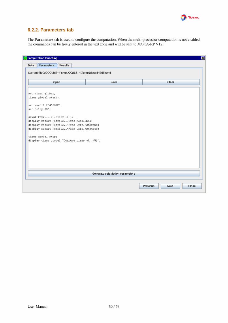
6.2.2. Parameters tab
The Parameters tab is used to configure the computation. When the multi-processor computation is not enabled,the commands can be freely entered in the text zone and will be sent to MOCA-RP V12.

User Manual 51 / 76
When the multi-processor computation is enabled, a zone appears above the text zone for configuring thecomputation (number of processors, number of histories, random generator seed, and maximum computation time).The text zone is simply used to add the commands necessary for the display.
6.2.3. Results tab
The Results tab initially launches the computations and then displays the results file (file type: ".res"). Fivefunctions are available here via buttons:
• open ".res" file;
• save current file;
• clear contents of current file;
• launch computations from graphical interface, a waiting window will be display, it allows to stop computationif need be;

User Manual 52 / 76
• launch computations in Batch mode to have permanent access to the input interface throughout thecomputations. Computations are launched with low priority.
6.3. Reading the results (former GUI)
A results file generated by MOCA-RP V12 can be divided into four parts (from top to bottom):

User Manual 53 / 76
1. The start of the file shows the general computation data. In addition, it gives the total time of the simulationand the number of histories simulated.
2. Results concerning the statistic states. They are classified by type of computation. Three values are shown foreach result:
• Mean value (m): this mean is computed on the number of simulated histories
• Standard deviation: gives an idea of the dispersion

User Manual 54 / 76
• 90% confidence interval (e): gives "e" such that the probability that the value "true" is between "m - e"and "m + e" is 0.9. Note: It is a good convergence indicator
In the above example the mean value of the statistic state called Stat1 is 0.99, the standard deviation is 3.64e-3and the confidence interval at 90% is 1.89e-3.
3. Mean frequency of the firings of all the Petri Nets transitions during a history. It is a result which issystematically returned by MOCA-RP V12.
In the above example, the mean firing frequency of the transition called Failure is 11.4.
4. 4. The following are supplied for each Petri Nets place (mean value and standard deviation):
• the "mean time" in the place (mean time during which the place contains one or more tokens);

User Manual 55 / 76
• the "mean number of tokens at the end of a history" in the place (mean marking of the place at the end ofa history).
These results are systematically returned by MOCA-RP V12
In the above example, the mean time spent in the Work place is 9901 hours (out of 10000 hours) with a standarddeviation of 36.4. The mean number of tokens at the end of a history is 0.99 with a standard deviation of 3.64e-3.
6.4. Reading the results (New GUI)
Since GRIF 2010, results are displayed in a windows with many tabs and tables.
6.4.1. Tables and Panels to display results
6.4.1.1. Result-tables
Result-tables are made of data and a top part to set table up.

User Manual 56 / 76
Columns can be sort by clicking on their header. The filter icon activates a filter set-up with the followingwindow:
When filter is activated, a small (+) is diplayed near column title. Filter can be remove with button.
6.4.1.2. Export data
Values that are visible in this table can be exported in CSV file format with button.
Results can also be displayed with a Curve by clicking on . Data used for x-axe and y-axe must be specifiedin the following window:
Then, chart is displayed in a window :

User Manual 57 / 76
Chart can be saved in the current document with the button at the bottom.
Nb : when chart is in document, points are no more modifiable.
6.4.1.3. Result-Panels
Result-panels have been created to facilitate data access in tables with many columns. The aim is to make a priorfilter to keep wanted data.
This panel is made of a combo-box in the upper-left corner which enables to remove the column from the tableand creates a list on the left which contains every values in the removed column. When you select a value in theleft list, it modifies the table in order to show lines whose removed column contains the selected value.
The combo-box in the upper-right corner enables to choose which column C will be used to cut table. The tablewill be cut in many tables, each one in a tab whose title is equal to the value used to filter the C column. Then Ccolumn is removed since it contains only the one value in a given tab.
6.4.2. Moca Results
Moca results atre displayed in a window containing 6 main tabs : variables, places, transitions, XML, stantardoutput, info.
6.4.2.1. Tab of Variables
The Variables tab contains every information computed for each variable (or statistical state).
• Value : Contains every value of a variable for every type of statistic.• History (at the end of histories) : contains historical values for each computed statitic.• Fixed size Histogram : Contains histograms computed by Moca (cf chapter about histograms)• Equiprobable classes Histogram : Contains histograms computed by Moca (cf chapter about histograms)• User defined Histogram : Contains histograms computed by Moca (cf chapter about histograms)• Timeline : Contains a timeline for each variable. Times are automatically computed by Moca.
6.4.2.2. Tab of Places
It contains sojourn duration and mean mark for each place of Petri Net.

User Manual 58 / 76
6.4.2.3. Tab of Transitions
It contains firing frequencies for each transition, and firing history for each history.
6.4.2.4. Other tabs
Other tabs display "raw" results. XML tab contains XML output of Moca, it is the file used to retrieve data. Thisfile can be used for further post-threatments.
Standard output display the standard output of Moca (available only afer computing).
Info tab contains usefull information about computation (simulation time, number of histories that have beendone ...)

User Manual 59 / 76
7. Curves
The curves can be drawn to study the model and the results better. To do this, click left on the corresponding iconon the vertical task bar then draw a box. This box will be the space assigned to displaying the curve(s). Initiallyit is only a white box with two axes without graduation.
Charts icon:
We must now define the curves to be drawn. To do this, click right on the box to display the Charts Edit window.
7.1. Charts Edit window
Note: It is important to specify that drawing curves requires a computation to be launched which is completelyindependent of that accessible in menu Data and computations - ....
The Charts Edit window is the same for all the GRIF modules
This window is divided into several parts:
1. Charts Title: allows you to give a title to the graphic.
User Manual 60 / 76
2. Data List: This part contains a three-column table listing the chart's different curves (name, description, display,curve colour, curve style, curve thickness).Several buttons are available above this table.• Recompute: launches or relaunches the computations necessary to draw the curves (this operation must be
performed each time the list of curves or the model is modified).•
Add : sends you to a Curve type window to add a curve to the chart (cf. following chapter).• Edit: modifies the selected curve.•
Delete : deletes the selected curve from the chart.•
Up : moves the selected curve upwards in the list.•
Down : moves the selected curve downwards in the list.• Save: the list of points computed for the selected curve in CSV format. This export doesn't contains generic
values. In order to export with generic values, use right-click and select Separate export.• Duplicate: creates a new curve identical to the selected curve.• Results: display in a text editor the results of the selected curve.
For each curve, you can specify its colour, its style of points, its thickness and its display options.
3. Computation options: allows you to configure the computation (optional depending on the module used).
4. Style: This part deals with displaying curves.• Style type: specifies the type of all the chart's curves (line or histogram).• Intervals on X and Y: Specifies the display interval for the X and Y axes (default interval or user-defined
interval). This last function can, for example, be used to zoom in on the most interesting parts of the curve.
The log check boxes are used to enable the logarithmic scale on the axis concerned. Important: 0 cannot berepresented on a log scale, remember to give a strictly positive starting point (e.g.: E-10). If 0 is given, thelog scale will start with an arbitrary value E-15.
When domain axe deals with time, you can choose time unit among : hours, days, months, years. Defaultdisplay is "hours" because it is the usualy used unit for modeling. It's only available in SIL module.
When computation engine allows it, you can display confidence range checking the checkbox.
With historam style, a checkbox allows to do a cumulated histogram.
5. Display options: enables (or not) the Display title function (displays the title of the chart) and the Displaygeneric values function (displays the min., max. and mean values of each curve).
When a curve is edited, its edition window contains 3 parts : times used for computation, target of computation,further information (generic values) that be be displayed or not under the curve.
Remark: it's sometimes useful to refresh all charts in document. Use the Tools / Refresh command or press F5
or icon.
7.2. Types of curves
When you click the Add button in the List of data part, a window is displayed called Type of curve. There arefour possibilities available:
• Moca 12 Curve: draws a totally conventional curve according to mean points computed during each history.
• Timing Chart: draws a curve according to points computed "intelligently" (the number of points computed isdirectly related to the size of the curve variations).
• Fixed Size Histogram: enumerates and classifies the results o btained at the end of a history in classes withfixed intervals.

User Manual 61 / 76
• Equiprobable Classes Histogram: according to the results on each history, determines the interval of thedifferent classes so that the probability of falling into each class is the same.
Note: an example of each type of curve will be presented later.
Whatever the type of curve selected, a window will be displayed allowing you to modify the computation timesand types.
The above window bears the name of the selected curve (in this case Moca 12 curve). It is divided into four parts:
1. Legend: used to give the curve a name.
2. Computation Time: the information to be specified in this part depends on the previously selected type ofcurve.
• Moca 12 Curve: interval and time step OR list of times (used to give the computation engine the exact pointsit must compute).
• Timing Chart: duration of a history (the computation engine will itself determine the points it mustcompute).
• Fixed Size Histogram: duration of a history AND number of intervals (the computation engine will nowonly have to perform enumeration and "storage" in each class).
• Equiprobable Classes Histogram: duration of a history AND number of equiprobable classes (thecomputation engine will determine the size of the classes).
• Defined Interval Histogram: duration of a history AND intervals to be used.
3. Default Statistics Type: allows you to choose the type of statistical computation on which the curve will becomputed. For the timing charts the curve automatically represents the statistic state value (type 3).
4. Target: used to select the statistical state on which the computations will be performed. These computationswill then be used to draw the curve..

User Manual 62 / 76
7.3. Examples of curves
Here are the Petri Nets from which the different curves will be drawn.
There are two components, A and B:
• A can be repaired with a delay before repair modelled by a Dirac law transition.
• B can also be repaired but with no delay before repair.
The simulation will be carried out for 10,000 histories of 30,000 hours.
7.3.1. Moca 12 Curve
This curve represents the change in mean availability of component A over time. The points have been computedat regular intervals (1 every 1000 hours).

User Manual 63 / 76
7.3.2. Timing Chart
This curve also represents the change in instantaneous availability of component A over time (marking of place no.1). In this case the points have been computed according to the curve variation. This "captures" the discontinuitiesbetter and thus makes the curve "smoother" and more precise.
7.3.3. Fixed Size Histogram
This histogram was produced from the mean value of the availability of component B (marking of place no. 5).The 10,000 results from the 10,000 simulated histories have been stored in 10 classes of the same interval.

User Manual 64 / 76
7.3.4. Equiprobable Classes Histogram
This histogram was produced from the mean value of the availability of component B (marking of place no. 5).Five equiprobable classes were requested. The probabilities that component B's mean availability is in one of theseclasses is identical.
7.3.5. Defined Interval Histogram
The 10,000 results from the 10,000 simulated histories have been stored in defined intervals. We have defined"[ 0,1,2,3" (equivalent to [0,1[ [1,2[ [2,3[ cf. Moca User Manual for more informations) We have computed numberof working components at the end of histories. We see that 2 components works at the end of histories most ofthe times. Intervals corresponding to S.I.L can be defined in order to see in wich S.I.L component is for differentstories.
Bounds of intervals can be defined as follows :
• Automaticaly defined limits for SIL• Manual definition of limits (separate by commas)• "Iteration" : user choose lower limit and upper limit, and the size of intervals.• "Iteration (log scale)" : user choose lower limit and upper limit, and the number of intervals. Size of intervals
will be computed in order to have same-size-intervals, on a logarithmic scale.
Moreover, two limits are added at minus infinity, and plus infinity, in order to have a chart containing every historyof the simulation.

User Manual 65 / 76
When limits are chosen, user has to choose between "left inclued" or "right included". Nb : IEC 61508 specifies"left included" intervals for SIL
7.3.6. Curve from existing results
Every curve previously shown, needs a computation for each chart. Computations can take a long time, that'swhy, since GRIF 20010, you can draw curves using results in a "Bank a results". This "Bank of results"contains previously made computations, there are saved for curve drawing and to re-display results without newcomputation.
Ediyion window of Curve from existing results allows to walk through the bank and find the wanted result. Thisresult comes from a computation which is already made, so, it is not possible to modify parameters (time, ...).
When result id selected, the bottom part of the window enables selection of data that will be used for x-axe, y-axe and confidence interval.

User Manual 66 / 76
8. Databases
In each GRIF module a connection can be established to a database. It is possible to have two different types ofconnections:
• connection to a CSV file;
• connection via a JDBC link.
8.1. Connection to a CSV file
8.1.1. Form of the database
This type of connection is the simplest to make. A CSV file has the extension ".csv". It is a simple text file wherethe different fields are separated by commas, tabs or semi-colons. It is the simplest form of database.
8.1.2. Connection
To connect GRIF to this database, go into menu Tools - Connection to a CSV file. A dialogue box is thendisplayed:
This window is divided into three parts:
• You must initially enter the path leading to the CSV file. To do this, there is an explorer available (... button).A Test function is used to check the connection.
• You must then enter the names of the four fields of the CSV file.
• Finally, specify the types of separators used in the CSV file.
Note: A CVS connection must be made with a CVS File (which means generated from only one sheet of a EXCELFile).

User Manual 67 / 76
8.2. Connection via a JDBC link (example with ODBC connector)
8.2.1. Form of the database
The database can initially be in the form of an EXCEL or ACCESS file. Then, using the operating system, anODBC system data source must be created. In the case of WINDOWS, for example, this operation is performed inmenu "Control Panel - Administration tools - data source (ODBC)". Here is an example of an EXCEL database:
8.2.2. Connection
To connect GRIF to this ODBC database, go into menu Tools - Application options - Database. A window isthen displayed which must be filled in as follows:
Notes:
1. sun.jdbc.odbc.JdbcOdbcDriver is the driver name
2. jdbc:odbc:REX specifies that "REX" is the name of the ODBC link
3. The fields Connection options, Login et Password are unnecessary here.
4. SELECT ID,NOM,VALEUR,DESCRIPTION FROM [Feuil1$] $] is called the query where Feuil1 is thename of the EXCEL sheet containing the data.

User Manual 68 / 76
8.3. Operation
The aim is now to link some of the model's parameters to the database. To do this, start by displaying the columnLinked to in the parameters table (click right on the top of the columns).
Then double click in the Linked to column to display the database items. When one of these items has beenselected, click OK to validate the connection. The parameter then takes the value of the item to which it is nowconnected.
Note: The button called Remove link to database at the bottom of the table breaks the link between the parameterand the database item.

User Manual 69 / 76
If some of the database values to which GRIF is linked are modified, the parameters connected to this databasecan be updated. To do this, select Data and computations - Update from database... and display the Databasewindow.
The parameters whose values are not up to date are automatically detected and indicated in bold. One or moreof these parameters can then be selected for updating using the Update selection button. Two other buttons areavailable to simplify the selection process: Unselect all (deselects all the table's parameters) and Select all (selectsall the table's parameters).
Remark: you can also directly copy parameter from database using menu Data and Computation/Database/Copyparameters from database. A window is displayed, you can select parameters you want to copy into document.Parameter will be automatically linked to the right paremeter in database.

User Manual 70 / 76
9. Save
Here is a summary of all the data which can be saved from a same model.
9.1. Model
It is obviously possible to save and reload the models which are made. To do this go into menu File - Save orinto File - Save as....
9.2. RTF File
A model can also be saved in RTF format. This allows the saved model to be reloaded in WORD to insert thegraphical part of the model in any document. To do this, go into menu File - Save in RTF file....
Note: There is another way to insert model in a report. Select the part of the model, copy it, and paste it in MicrosoftWORD or other software.

User Manual 71 / 76
9.3. Input data
When the input data for the computation engine is generated, it can be saved. This type of file has the ".don"extension. These files can therefore be modified using a text editor then reloaded to launch computations on them(for example). This action should be made only by advanced user.
9.4. Results file
The results file can also be saved. This type of file has the ".res" extension. These files can therefore be reloadedinto another program (e.g. EXCEL) to exploit the results in more detail.
9.5. Curves
For each curve drawn, the points which have been computed in CSV format can be saved. This list of points canthen be used to draw new curves or to perform further computations.

User Manual 72 / 76
9.6. Tables
The input tables designed for complex and elaborate computations can be imported and exported. To do this, gointo menu Data and computations - Import data or into Data and computations - Export data.
User Manual 73 / 76
10. Options of GRIF - Petri Nets withpredicates
Tools - Application Options menu opens a window containing the following tabs:
10.1. Executables
Executables tab enables to specify path to external executables :
• Editor path : Specifies text editor path.• Automatically open PDF files : Specifies if PDF reports must be openned avec generation.• Style-sheet from XML to DocBook. : Style-sheet allowing converting from XML report to docbook file.• Style-sheet from XML to HTML. : Style-sheet allowing converting from XML report to HTML file.• Style-sheet from DocBook to PDF. : Style-sheet allowing converting from docbook file to PDF file.• Moca-RPC path : Specifies path of Moca 10.
10.2. Database
Database tab enables to configure database connection :
• Use DataBase connection for parameters : Select if database must be use.• Name : Database name will be put into parameter during its update. It enables to know from which database
parameter has been lastly updated.• JDBC Driver : Enter name of JDBC driver to be used(sun.jdbc.odbc.JdbcOdbcDriver,
oracle.jdbc.driver.OracleDriver, ...).• Connection to database : Database Url.• Connection options : Connection properties.• Login : Login to be used to connect to database.• Password : Password to be used to connect to database.• SQL Request : Request that have to be executed to retrieve data from database.• Name of "ID" field : Name of field containing data ID.• Type of ID : Type of ID field (INTEGER, FLOAT, VARCHAR(32), ...)• Name of "name" field : Name of field containing data name.• Name of "value" field : Name of field containing data value.• Name of "description" field : Name of field containing data description.• Test Connection : Name of field containing data description.
10.3. Language
Language tab enables to choice language :
• Language : Language changes are taken into account when option windows is closed.Available language areFrench and English.
10.4. Options
Options tab enables to tune application behavior :
• Save working document options as default options in application : Save options of current doc as applicationdefault options.
• Application manage default options of documents. Apply defaut options to current document : Apply -Application options- to current document.
• Number of undo : Specifies number of possible undo/redo.

User Manual 74 / 76
• Number of recent files : Specifies number of files in recent files list.• Window display : Enables separate tables (external) or linked tables (internal).• Columns to be resized in tables : Enables to specify the columns on which space will be taken for resizing.• Use net protection key (Red) : Check this box only if a network key is used (reg key).• Manage new names to avoid name conflict : Tries to avoid name conflict, creating new objects whose name
is unik (when pasting for example).• Synchronise view with tables : Select objects in tables (on the right) when they are selected in view.• Synchronise view with explorer : Select objects in explorer (on the left) when they are selected in view.• Ask for configuration of observed variables : Ask for computation setup when variable becomes observed.
10.5. Graphics
Graphics tab enables to modify GUI look :
• Element Zoom : Changes graphics size.• Comment size : Changes comment font size.• Activate cross hair : Activate cross hair which enables object alignment.• Activate smoothing for texts : Activate anti-aliasing (smoothing) for texts, it can slow the display.• Activate smoothing for images : Activate anti-aliasing (smoothing) for images, it can slow the display.• Activate tooltips : Activate tooltip-system.• Draw places and transitions according IEC 62522 PN Techniques : Draw places and transitions according
IEC 62522. Transitions will be drawn depending on their law.
10.6. Digital format
Digital format tab enables to customize digits display :
• Display of parameters : Specifies the display of parameters (number of digits, ...).
10.7. Places
Places tab defines places display options. :
• Label size : Specifies size of places font.• Display name : Enables to display place name or not.• Display number : Enables to display place ID or not.• Display number of tokens : Enables to display number of tokens or not.• Display name on shortcuts : Enables to display the name of reference place on each shortcut.
10.8. Transitions
Transitions tab defines Transitions display options :
• Label size : Specifies size of transitions font.• Display name : Enables to display transition name or not.• Display number : Enables to display transition ID or not.• Show HISTO characteristics : Enables to display HST flag of transition or not.• Display firing options (PRIO, EQP ...) : Enables to display firing options of transitions.• Display SEQ flag if needed : Enables to display SEQ flag for transitions with sequential assignments.• Display guards : Enables to display guards of transition or not.• Display assignment : Enables to display assignments of transition or not.• Display law : Enables to display law of transition or not.• Use a default law : Enables to use a specific law as default law.• Default law : Enables to define the default law to be used.• Maximum number of characters by line : Specifies maximum number of characters per line.• Lexical check before computing : Activate lexical check of transitions before each computation.

User Manual 75 / 76
10.9. Arcs
Arcs tab defines arcs display options :
• Label size : Specifies label font size.• Link arrow width : Specifies arrow width.• Link arrow height : Specifies arrow height.• Display arc weight : Enables to display arcs weight or not.
10.10. Local data
Local data tabs enables to change local data display :
• Label size : Specifies label font size.• Display data name : Display data name.• Display data domain : Display domain of definition.• Display data definition : Display variable definition.• Display data value : Display data value.
10.11. Simulation
Simulation tab enables to set simulation up :
• Automatic firing of dirac 0 : Automatic firing of transition with Dirac 0 law.• Automatic firing when simulation starts : Automatic firing of transition when simulation starts.• Transitions fireable before loop detection : Specifies maximum number of fire before loop detection.• Graphical Rendering of simulation : Activate or not graphical rendering of simulation or each modification.• Delay between transition fire : Delay between two automatic fire.• Simulation trace : Enable simulation trace.• Path to trace file : File where simulation is saved.• Choose the wayt to fire transition with "on demand" type : Displays a dialog box when firing "on demand"
transition.• Follow scheduler order for deterministic transitions : Only the fisrt deterministic transition of scheduler
can be fired.• Choose delay of fired transitions : Displays a dialog box to choose delay of fired transition.• Uncertainty propagation for interactiv simulation : If not checked, the value of variable with uncertainty
will be the average. For example, 1.5 for a unif(1,2).• Unlimited histogram : Enables full histogramme.• Display histogram (transition) : Enables to choice type of histogramme for transitions.• Parameter (nb classes, nb and size of steps ...) : Specifies parameter for transition histograms.
10.12. Prototypes
Prototypes tab contains options of prototypes. :
• Verify compatibility with Stochastic bloc module : Verifies compatibility of generated blocks with Stochasticbloc module
• Path of the directory of the prototype library : Directory where are saved prototypes of Petri12 library.
10.13. Curves
Charts tab enables to change charts drawing :
• Set graphics borders : Add borders to charts.• Set generic values borders : Add borders to generic values under charts.• Display grid : Display grid on curves area.• Display legends : Display legends under curves.

User Manual 76 / 76
• Drawing zone transparency : Activate curves area transparency.• Graphic transparency : Activate charts transparency.• Title size : Specifies charts title font size.• Generic values size : Specifies generic values font size.• Point size : Specifies point size on curves.• Coordinates size : Specifies coordinates font size.• Legend size : Specifies legends font size.• Max number of points : Specifies maximum number of points to be drawn.• Max number of points to save : Specifies maximum number of points to be saved.• Draw S.I.L : Horizontal lines are drawn at E-1 E-2 E-3 E-4.• Save points in document : Specifies if points of charts have to be saved in document.• Vertical abscise for histogram. : Display coordinate of abscise verticaly.