greenhouse gas fluxes derived from regional measurement

Greenhouse gas fluxes derived from regional

measurement networks and atmospheric

inversions: Results from the MCI and INFLUX experiments

Kenneth Davis

The Pennsylvania State University

and

The INFLUX and MCI research teams

Megacities workshop, Pasadena, CA, 8 May, 2012

Earth

Networks

• Or:

– Paul: Airplanes

– Ken: Towers

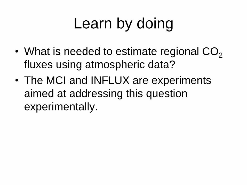
Learn by doing

• What is needed to estimate regional CO2

fluxes using atmospheric data?

• The MCI and INFLUX are experiments

aimed at addressing this question

experimentally.

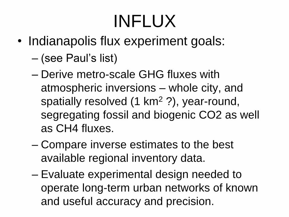
INFLUX • Indianapolis flux experiment goals:

– (see Paul’s list)

– Derive metro-scale GHG fluxes with

atmospheric inversions – whole city, and

spatially resolved (1 km2 ?), year-round,

segregating fossil and biogenic CO2 as well

as CH4 fluxes.

– Compare inverse estimates to the best

available regional inventory data.

– Evaluate experimental design needed to

operate long-term urban networks of known

and useful accuracy and precision.

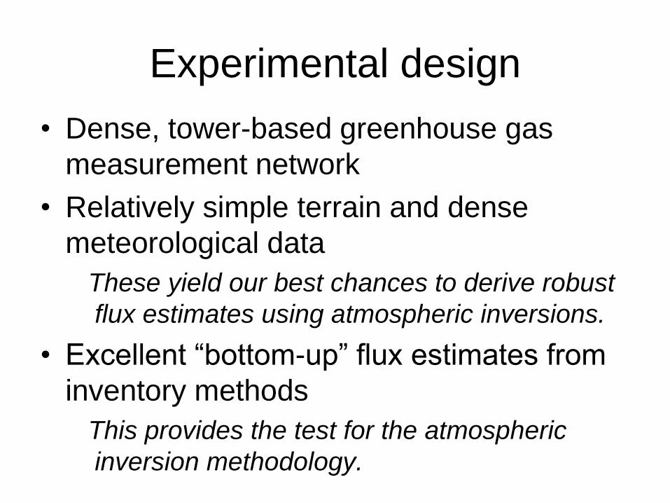
Experimental design

• Dense, tower-based greenhouse gas

measurement network

• Relatively simple terrain and dense

meteorological data

These yield our best chances to derive robust

flux estimates using atmospheric inversions.

• Excellent “bottom-up” flux estimates from

inventory methods

This provides the test for the atmospheric

inversion methodology.

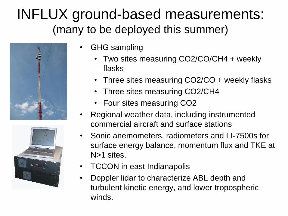
INFLUX ground-based measurements: (many to be deployed this summer)

• GHG sampling

• Two sites measuring CO2/CO/CH4 + weekly

flasks

• Three sites measuring CO2/CO + weekly flasks

• Three sites measuring CO2/CH4

• Four sites measuring CO2

• Regional weather data, including instrumented

commercial aircraft and surface stations

• Sonic anemometers, radiometers and LI-7500s for

surface energy balance, momentum flux and TKE at

N>1 sites.

• TCCON in east Indianapolis

• Doppler lidar to characterize ABL depth and

turbulent kinetic energy, and lower tropospheric

winds.

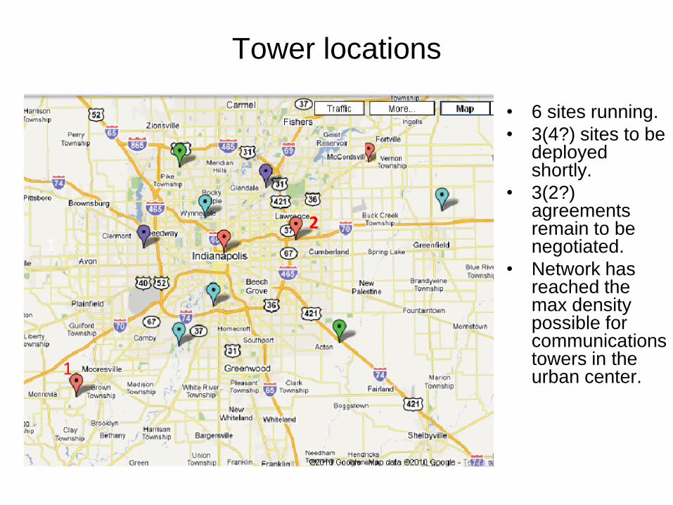
Tower locations

• 6 sites running.

• 3(4?) sites to be deployed shortly.

• 3(2?) agreements remain to be negotiated.

• Network has reached the max density possible for communications towers in the urban center.

1

2 1

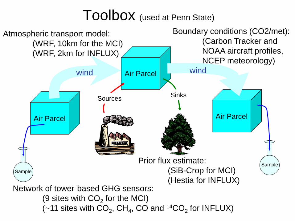
Toolbox (used at Penn State)

Air Parcel Air Parcel

Air Parcel

Sources Sinks

wind wind

Sample

Sample

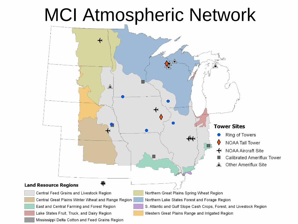
Network of tower-based GHG sensors:

(9 sites with CO2 for the MCI)

(~11 sites with CO2, CH4, CO and 14CO2 for INFLUX)

Atmospheric transport model:

(WRF, 10km for the MCI)

(WRF, 2km for INFLUX)

Prior flux estimate:

(SiB-Crop for MCI)

(Hestia for INFLUX)

Boundary conditions (CO2/met):

(Carbon Tracker and

NOAA aircraft profiles,

NCEP meteorology)

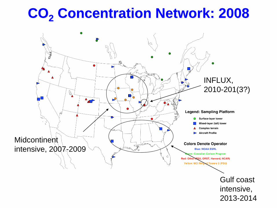
CO2 Concentration Network: 2008

Midcontinent

intensive, 2007-2009

INFLUX,

2010-201(3?)

Gulf coast

intensive,

2013-2014

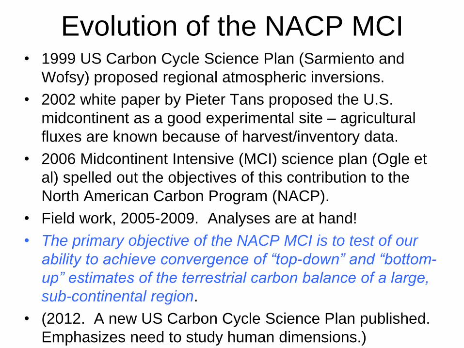
Evolution of the NACP MCI • 1999 US Carbon Cycle Science Plan (Sarmiento and

Wofsy) proposed regional atmospheric inversions.

• 2002 white paper by Pieter Tans proposed the U.S.

midcontinent as a good experimental site – agricultural

fluxes are known because of harvest/inventory data.

• 2006 Midcontinent Intensive (MCI) science plan (Ogle et

al) spelled out the objectives of this contribution to the

North American Carbon Program (NACP).

• Field work, 2005-2009. Analyses are at hand!

• The primary objective of the NACP MCI is to test of our

ability to achieve convergence of “top-down” and “bottom-

up” estimates of the terrestrial carbon balance of a large,

sub-continental region.

• (2012. A new US Carbon Cycle Science Plan published.

Emphasizes need to study human dimensions.)

MCI Atmospheric Network

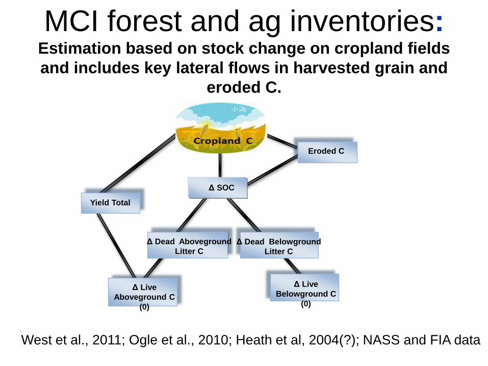
Δ SOC

Yield Total

Eroded C

Δ Live

Aboveground C

(0)

Δ Dead Aboveground

Litter C

Δ Dead Belowground

Litter C

Δ Live

Belowground C

(0)

MCI forest and ag inventories: Estimation based on stock change on cropland fields

and includes key lateral flows in harvested grain and

eroded C.

West et al., 2011; Ogle et al., 2010; Heath et al, 2004(?); NASS and FIA data

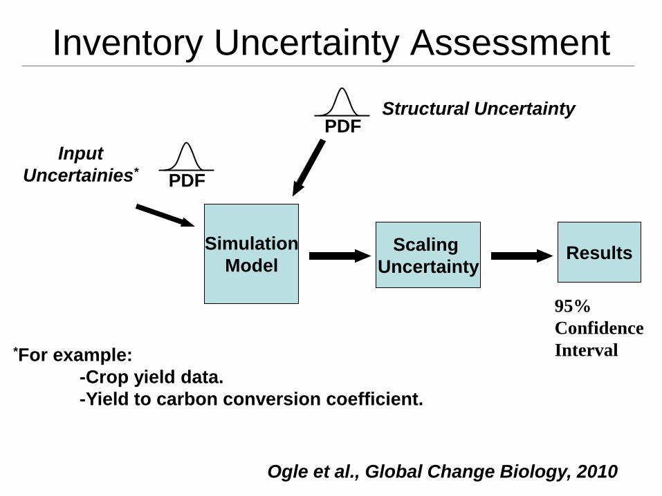
Inventory Uncertainty Assessment

Simulation

Model

PDF

Scaling

Uncertainty Results

Structural Uncertainty PDF

95%

Confidence

Interval

Input

Uncertainies*

Ogle et al., Global Change Biology, 2010

*For example:

-Crop yield data.

-Yield to carbon conversion coefficient.

Lessons from the NACP MCI

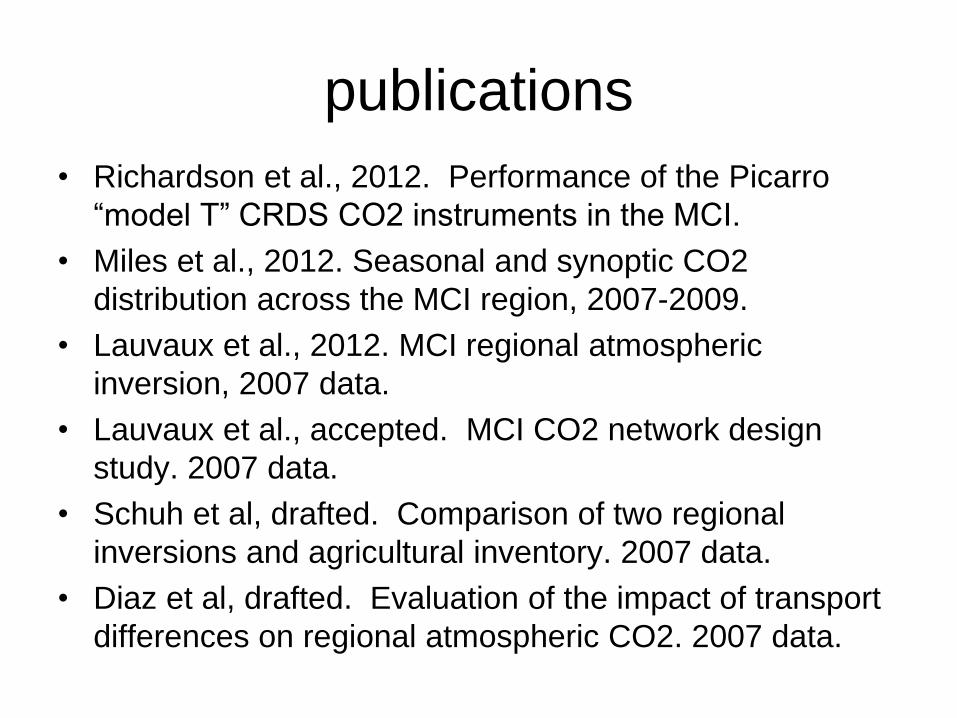
publications

• Richardson et al., 2012. Performance of the Picarro

“model T” CRDS CO2 instruments in the MCI.

• Miles et al., 2012. Seasonal and synoptic CO2

distribution across the MCI region, 2007-2009.

• Lauvaux et al., 2012. MCI regional atmospheric

inversion, 2007 data.

• Lauvaux et al., accepted. MCI CO2 network design

study. 2007 data.

• Schuh et al, drafted. Comparison of two regional

inversions and agricultural inventory. 2007 data.

• Diaz et al, drafted. Evaluation of the impact of transport

differences on regional atmospheric CO2. 2007 data.

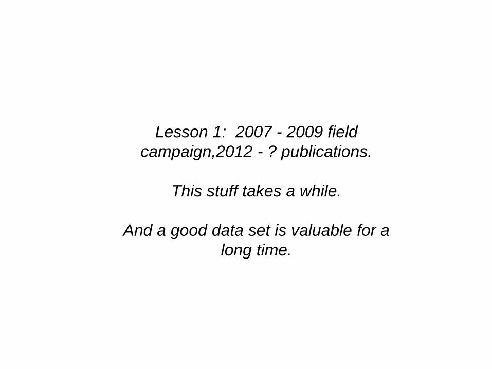
Lesson 1: 2007 - 2009 field

campaign,2012 - ? publications.

This stuff takes a while.

And a good data set is valuable for a

long time.

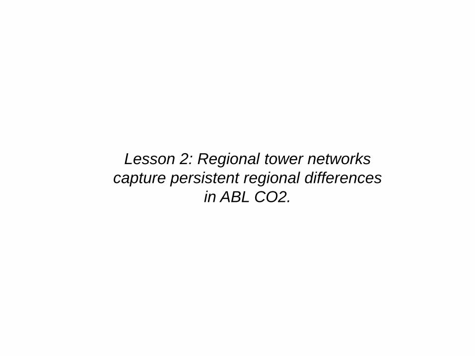
Lesson 2: Regional tower networks

capture persistent regional differences

in ABL CO2.

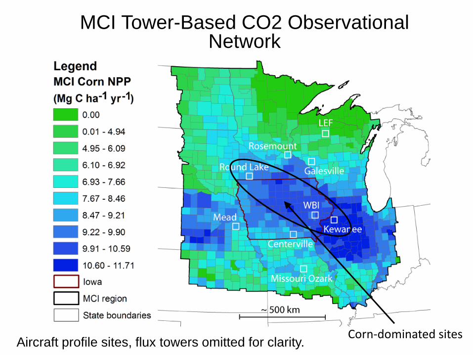
Corn-dominated sites

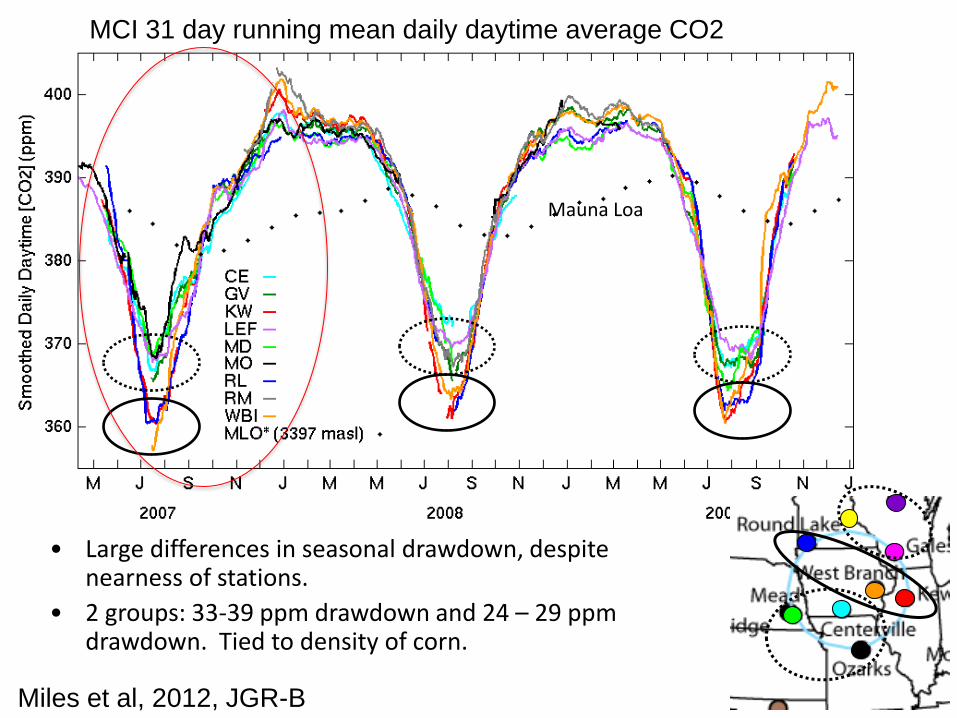
MCI Tower-Based CO2 Observational Network

Aircraft profile sites, flux towers omitted for clarity.

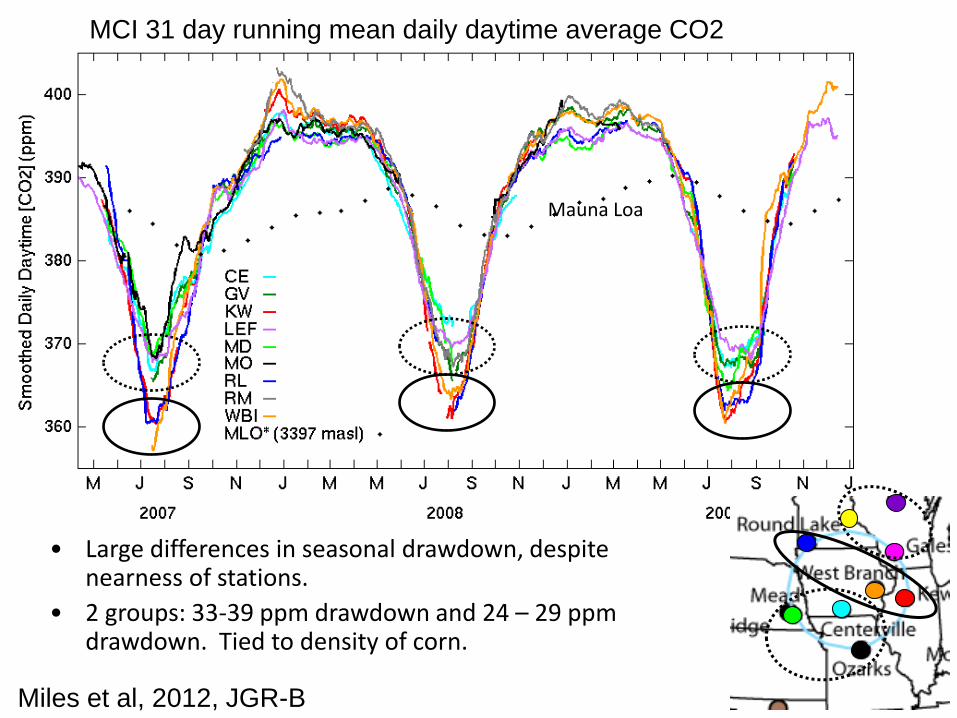
• Large differences in seasonal drawdown, despite nearness of stations.

• 2 groups: 33-39 ppm drawdown and 24 – 29 ppm drawdown. Tied to density of corn.

Mauna Loa

Miles et al, 2012, JGR-B

MCI 31 day running mean daily daytime average CO2

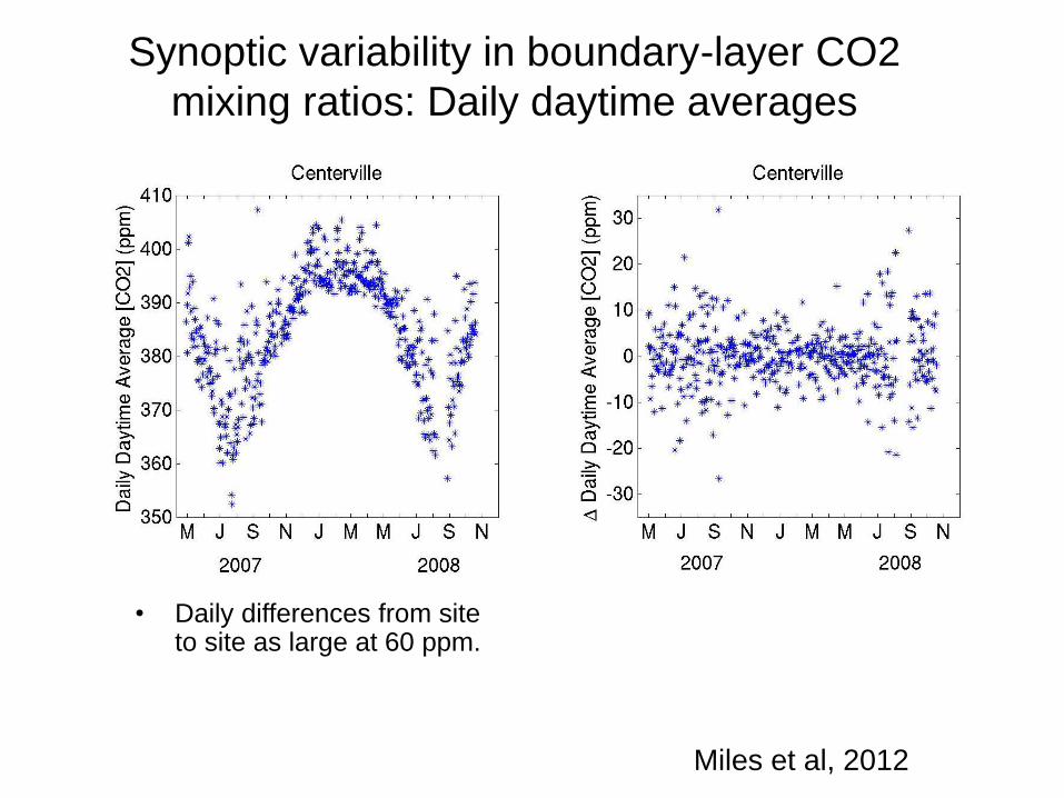
• Daily differences from site to site as large at 60 ppm.

Synoptic variability in boundary-layer CO2

mixing ratios: Daily daytime averages

Miles et al, 2012

Lesson 3: 2007 MCI flux estimates

appear to converge.

Success?

• Large differences in seasonal drawdown, despite nearness of stations.

• 2 groups: 33-39 ppm drawdown and 24 – 29 ppm drawdown. Tied to density of corn.

Mauna Loa

Miles et al, 2012, JGR-B

MCI 31 day running mean daily daytime average CO2

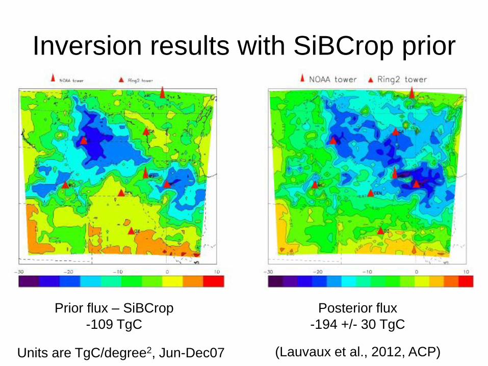
Inversion results with SiBCrop prior

Prior flux – SiBCrop

-109 TgC

Posterior flux

-194 +/- 30 TgC

Units are TgC/degree2, Jun-Dec07 (Lauvaux et al., 2012, ACP)

Inversion results with CT prior

Prior flux – CT posterior

-198 TgC

Posterior flux

-215 +/- 30 TgC

Units are TgC/degree2, Jun-Dec07 (Lauvaux et al., 2012, ACP)

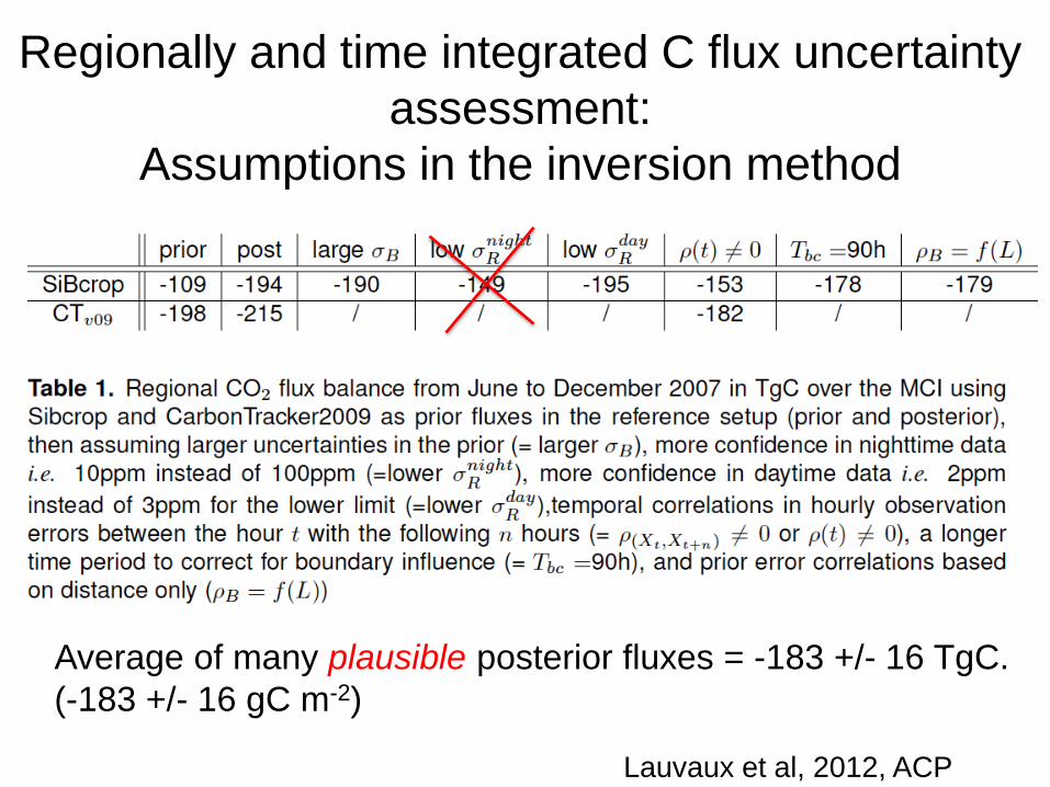
Regionally and time integrated C flux uncertainty

assessment:

Assumptions in the inversion method

Lauvaux et al, 2012, ACP

Average of many plausible posterior fluxes = -183 +/- 16 TgC.

(-183 +/- 16 gC m-2)

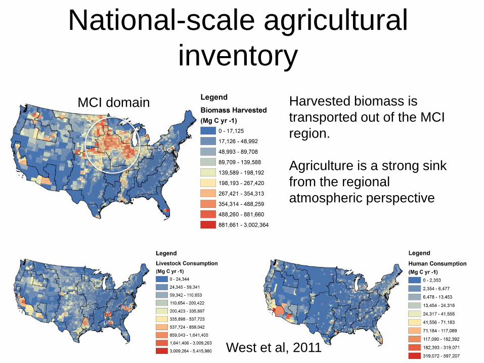
National-scale agricultural

inventory

26

Harvested biomass is

transported out of the MCI

region.

Agriculture is a strong sink

from the regional

atmospheric perspective

West et al, 2011

MCI domain

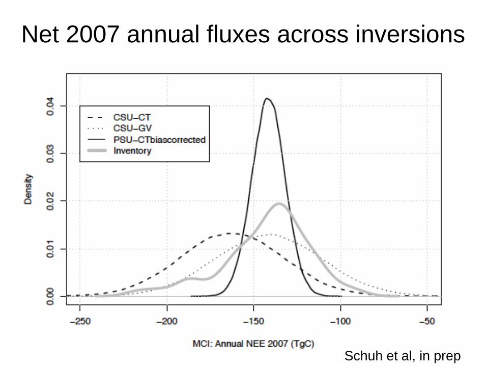
Net 2007 annual fluxes across inversions

Schuh et al, in prep

Lesson 4: Measuring GHG boundary

conditions is very important/critical

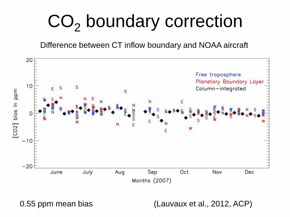
CO2 boundary correction

(Lauvaux et al., 2012, ACP) 0.55 ppm mean bias

Difference between CT inflow boundary and NOAA aircraft

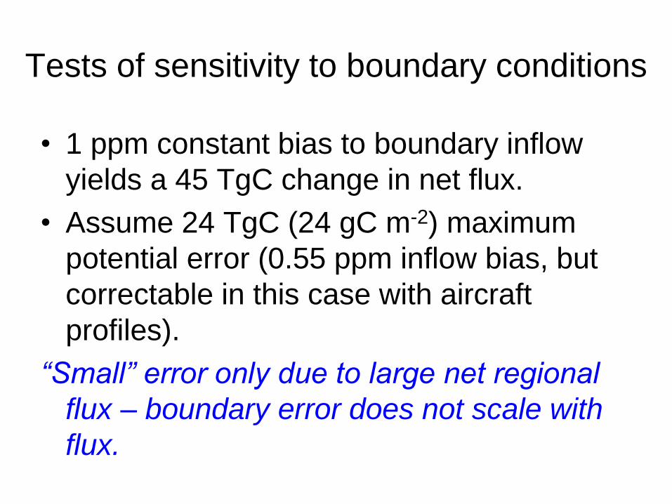
Tests of sensitivity to boundary conditions

• 1 ppm constant bias to boundary inflow

yields a 45 TgC change in net flux.

• Assume 24 TgC (24 gC m-2) maximum

potential error (0.55 ppm inflow bias, but

correctable in this case with aircraft

profiles).

“Small” error only due to large net regional

flux – boundary error does not scale with

flux.

Lesson 5: The MCI network was more

than sufficient for determining the

regionally aggregated CO2 flux and

barely(?) sufficient for determining

spatial patterns in CO2 flux.

Regional NEE of CO2

for various subsets of

the MCI network,

2007.

Spatial pattern of NEE

is sensitive to the

network choice.

Lauvaux et al, accepted

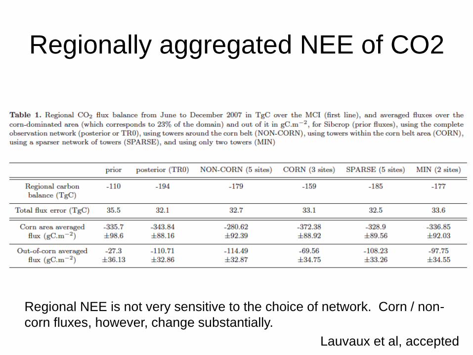
Regionally aggregated NEE of CO2

Regional NEE is not very sensitive to the choice of network. Corn / non-

corn fluxes, however, change substantially.

Lauvaux et al, accepted

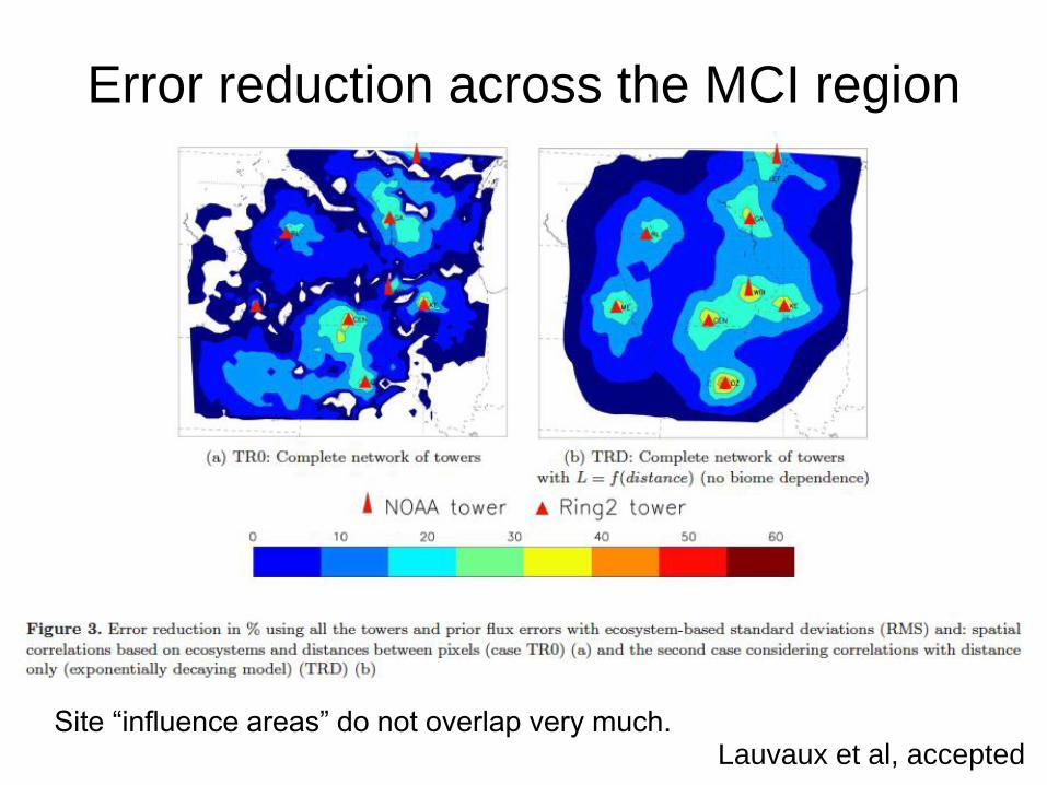
Error reduction across the MCI region

Site “influence areas” do not overlap very much. Lauvaux et al, accepted

Lesson 6: Atmospheric transport

matters a lot.

(Influence on inverse flux estimates has

yet to be properly evaluated.)

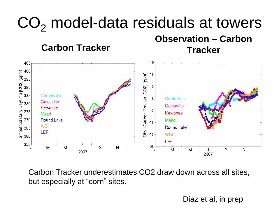
CO2 model-data residuals at towers

Carbon Tracker Observation – Carbon

Tracker

Carbon Tracker underestimates CO2 draw down across all sites,

but especially at “corn” sites.

Diaz et al, in prep

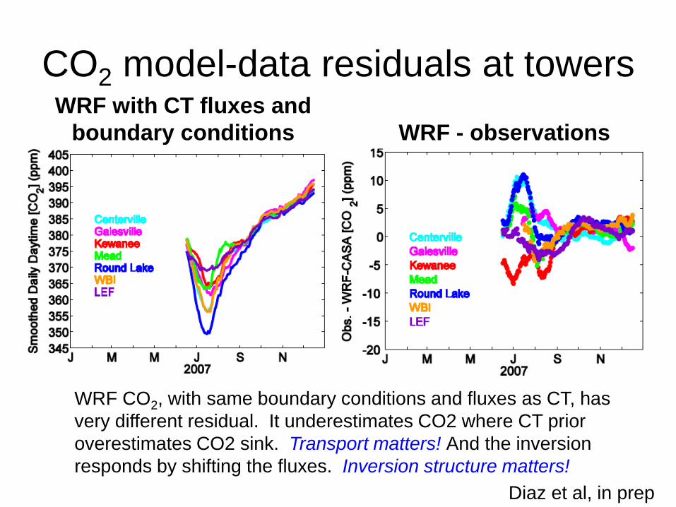
CO2 model-data residuals at towers WRF with CT fluxes and

boundary conditions WRF - observations

WRF CO2, with same boundary conditions and fluxes as CT, has

very different residual. It underestimates CO2 where CT prior

overestimates CO2 sink. Transport matters! And the inversion

responds by shifting the fluxes. Inversion structure matters!

Diaz et al, in prep

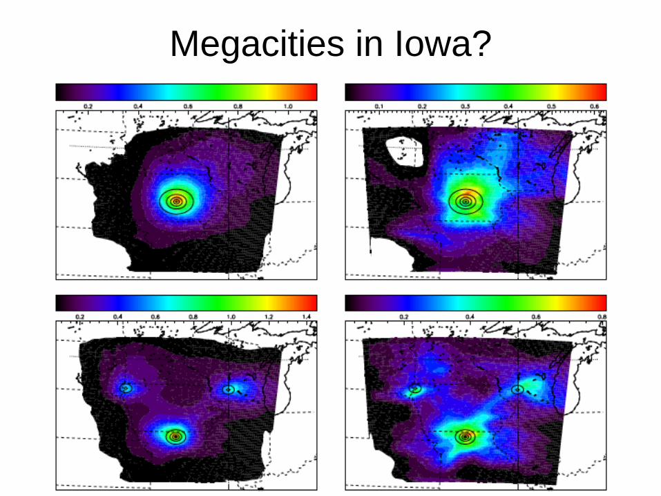
Megacities in Iowa?

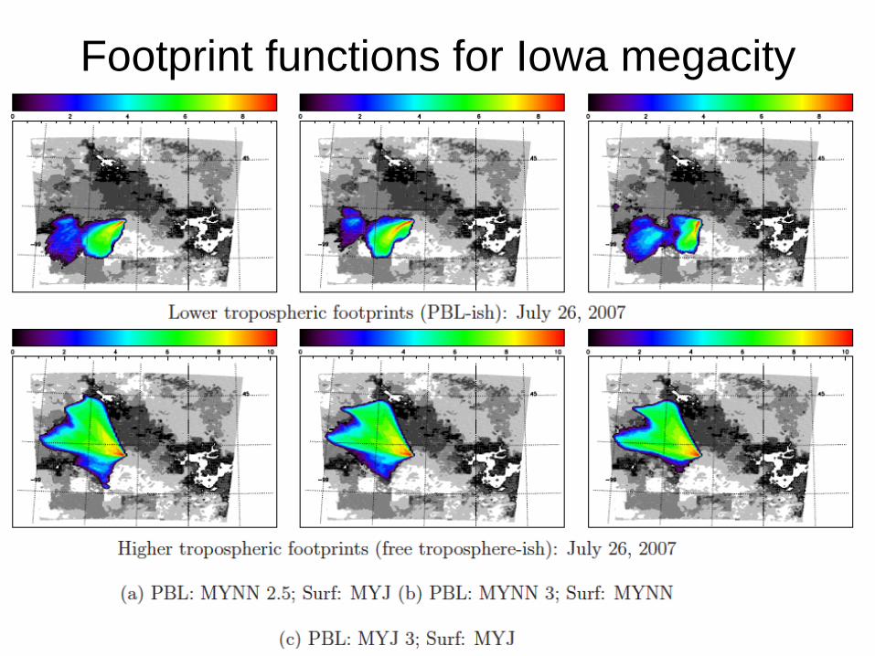
Footprint functions for Iowa megacity

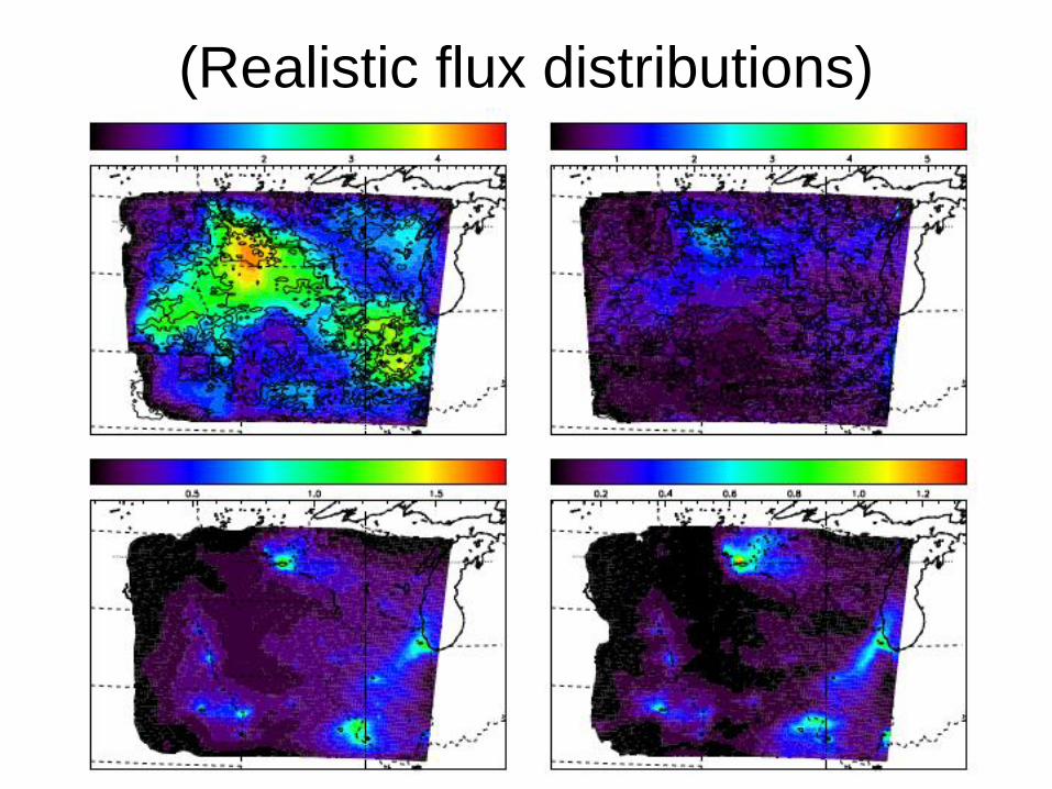
(Realistic flux distributions)

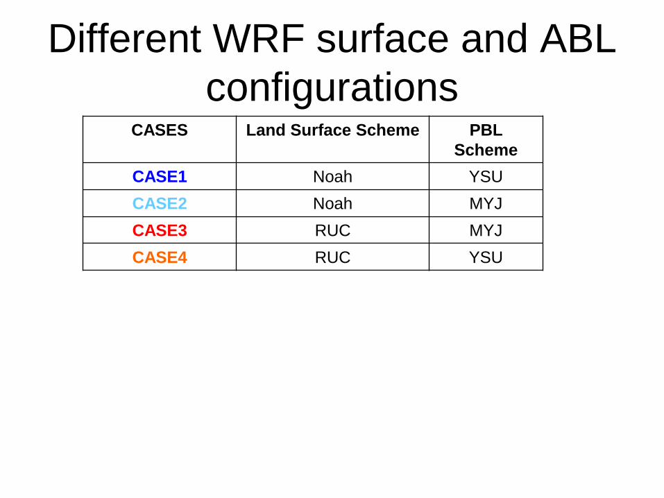
Different WRF surface and ABL

configurations CASES Land Surface Scheme PBL

Scheme

CASE1 Noah YSU

CASE2 Noah MYJ

CASE3 RUC MYJ

CASE4 RUC YSU

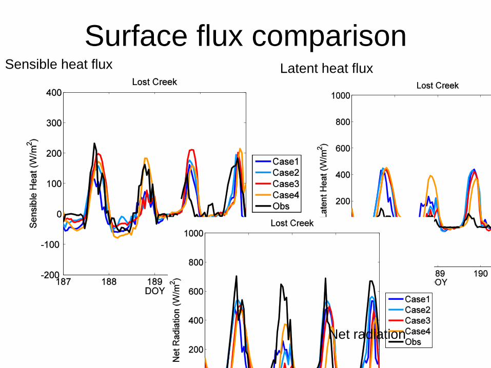
Surface flux comparison Sensible heat flux Latent heat flux

Net radiation

Lessons from INFLUX (to date)

Lesson 1: Setting up a dense observational

network takes significant time (2010 – 2012) and

resources. Don’t do this lightly. Or drop the data

set quickly.

Lesson 2: Maintaining a consistent data stream

from those observational assets is challenging

(e.g. phone lines, computer hang-ups, pump

failures…)

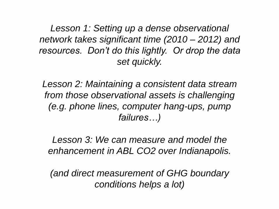
Lesson 3: We can measure and model the

enhancement in ABL CO2 over Indianapolis.

(and direct measurement of GHG boundary

conditions helps a lot)

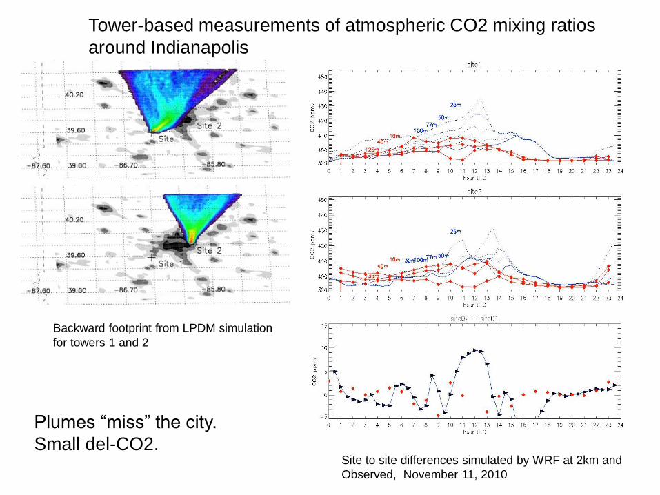
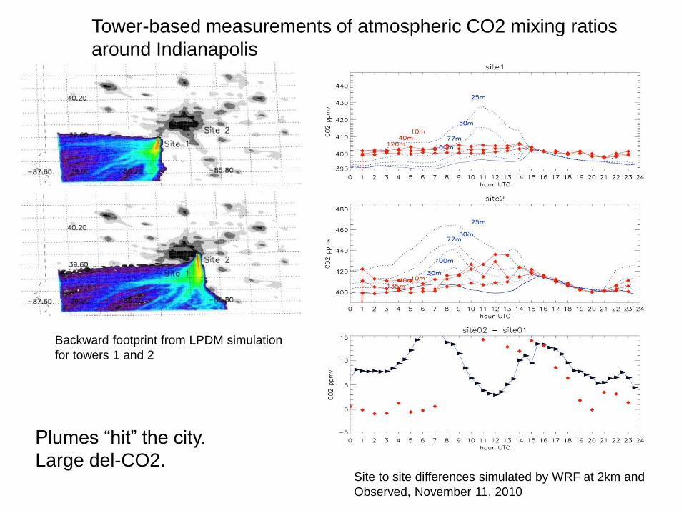
Backward footprint from LPDM simulation

for towers 1 and 2

Site to site differences simulated by WRF at 2km and

Observed, November 11, 2010

Tower-based measurements of atmospheric CO2 mixing ratios

around Indianapolis

Plumes “miss” the city.

Small del-CO2.

Site to site differences simulated by WRF at 2km and

Observed, November 11, 2010


for towers 1 and 2

Tower-based measurements of atmospheric CO2 mixing ratios

around Indianapolis

Plumes “hit” the city.

Large del-CO2.

Lesson 4: The INFLUX network should provide

good coverage/detectability for metro GHG fluxes.

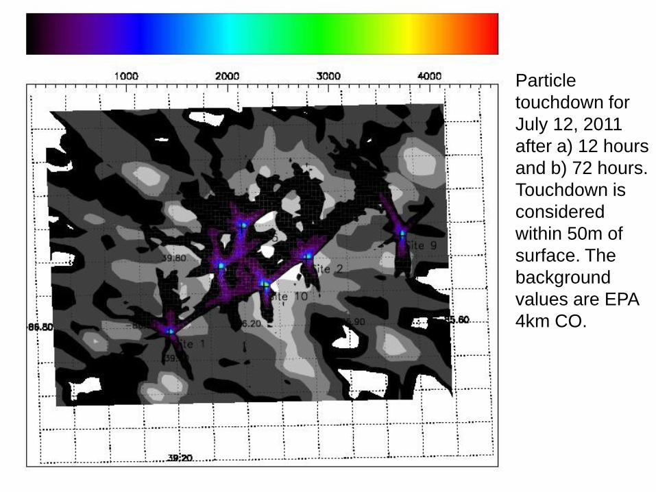
Particle

touchdown for

July 12, 2011

after a) 12 hours

and b) 72 hours.

Touchdown is

considered

within 50m of

surface. The

background

values are EPA

4km CO.

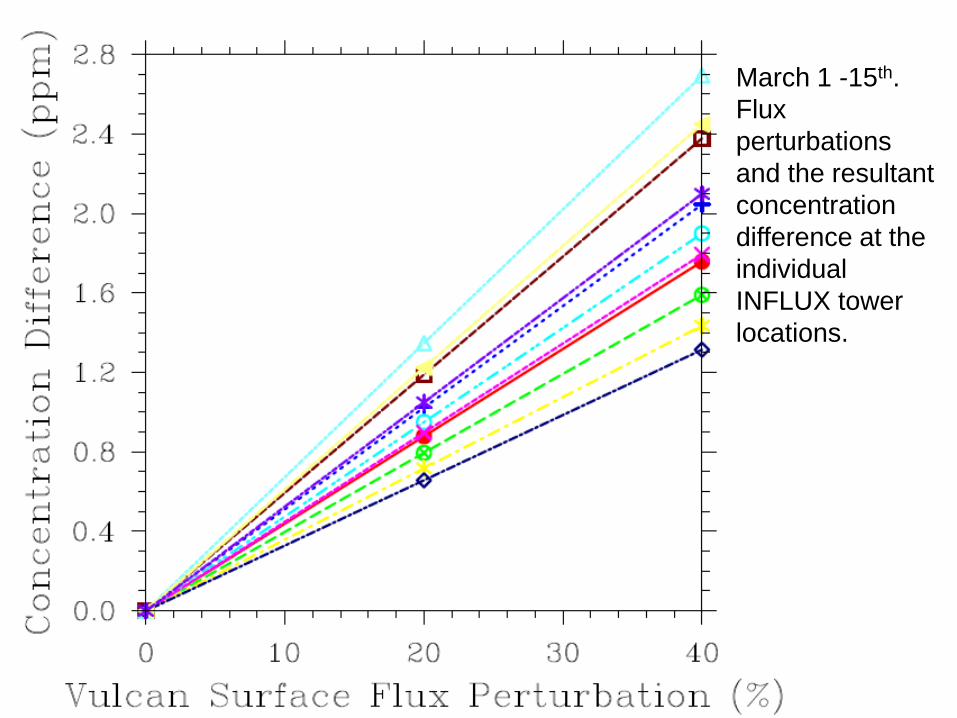
March 1 -15th.

Flux

perturbations

and the resultant

concentration

difference at the

individual

INFLUX tower

locations.

Lesson 5: Large point sources are important. Get

strong priors for them.

(and transport matters)

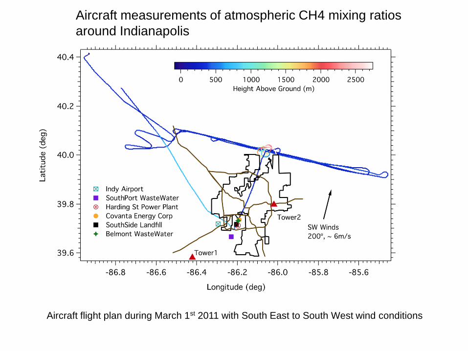
Aircraft measurements of atmospheric CH4 mixing ratios

around Indianapolis

Aircraft flight plan during March 1st 2011 with South East to South West wind conditions

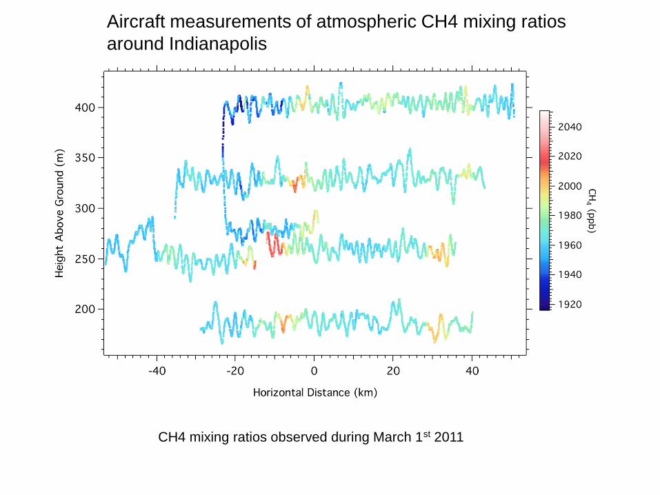
CH4 mixing ratios observed during March 1st 2011


around Indianapolis

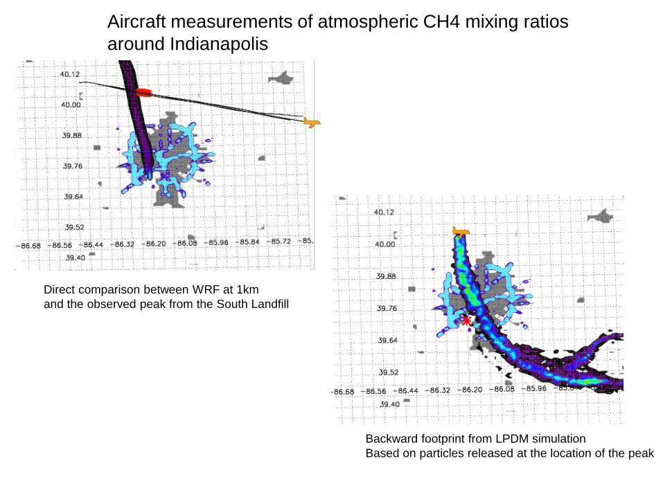
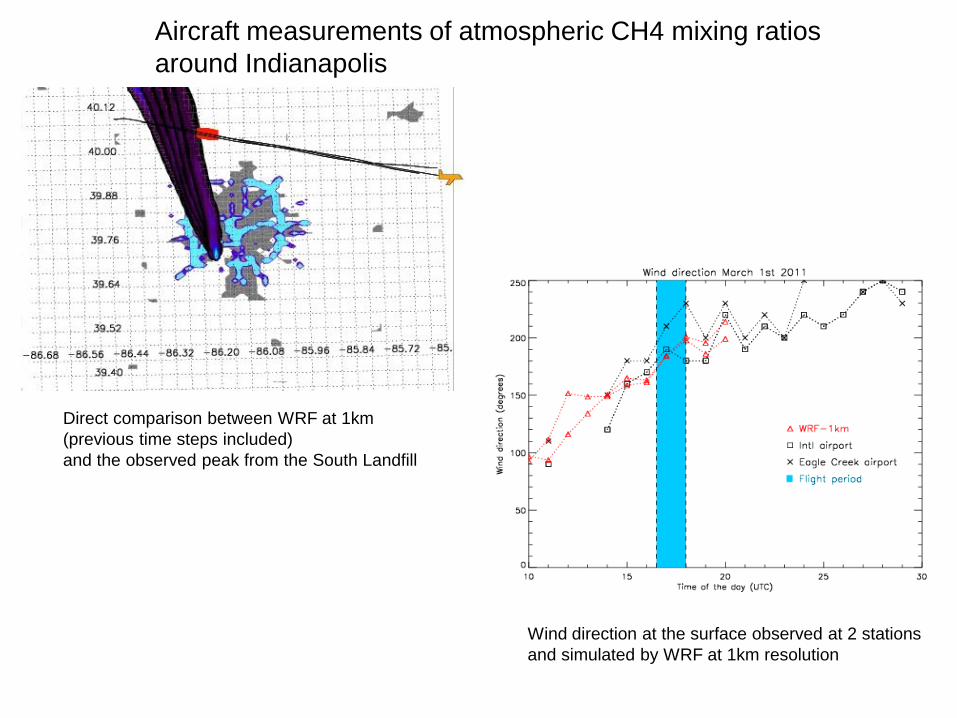
Direct comparison between WRF at 1km

and the observed peak from the South Landfill


Based on particles released at the location of the peak


around Indianapolis

Direct comparison between WRF at 1km

(previous time steps included)

and the observed peak from the South Landfill

Wind direction at the surface observed at 2 stations

and simulated by WRF at 1km resolution


around Indianapolis

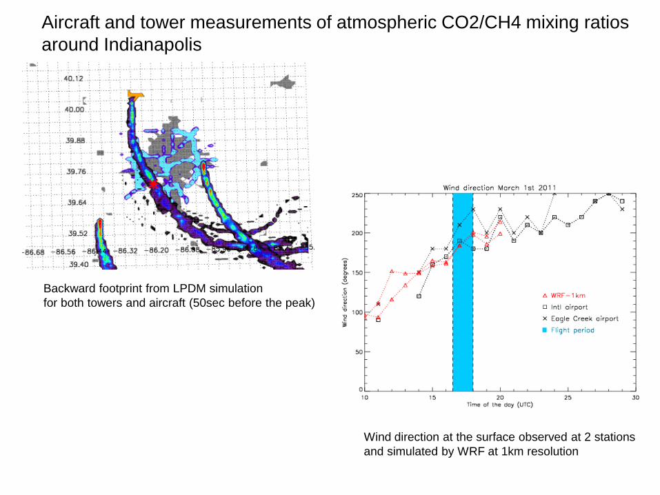
Aircraft and tower measurements of atmospheric CO2/CH4 mixing ratios

around Indianapolis


for both towers and aircraft (50sec before the peak)

Wind direction at the surface observed at 2 stations

and simulated by WRF at 1km resolution

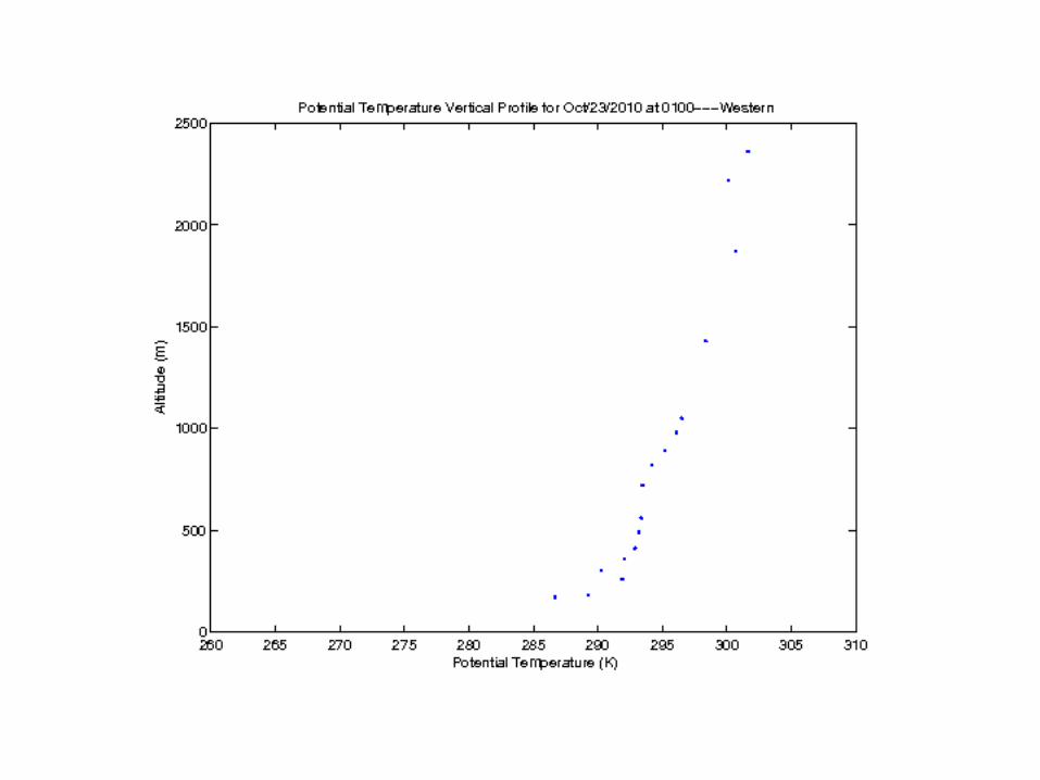
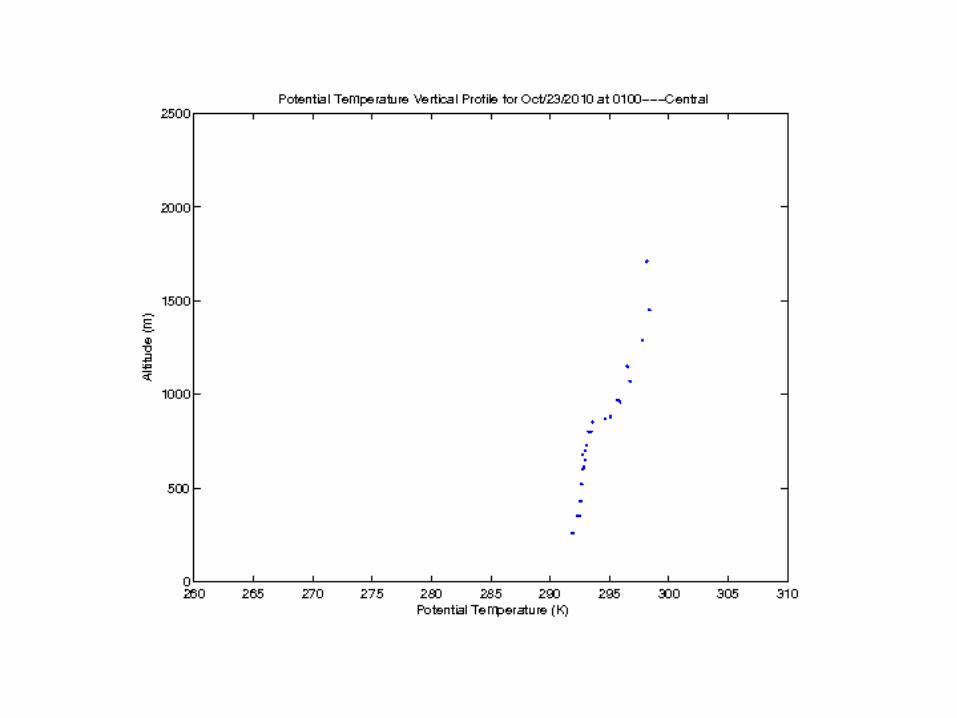
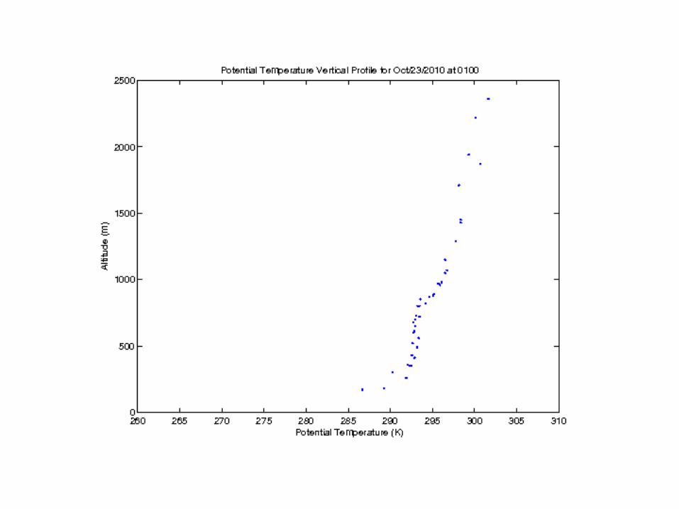
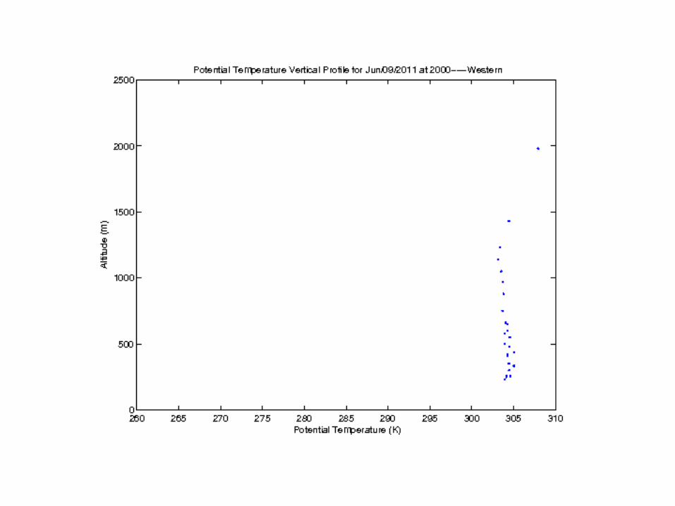
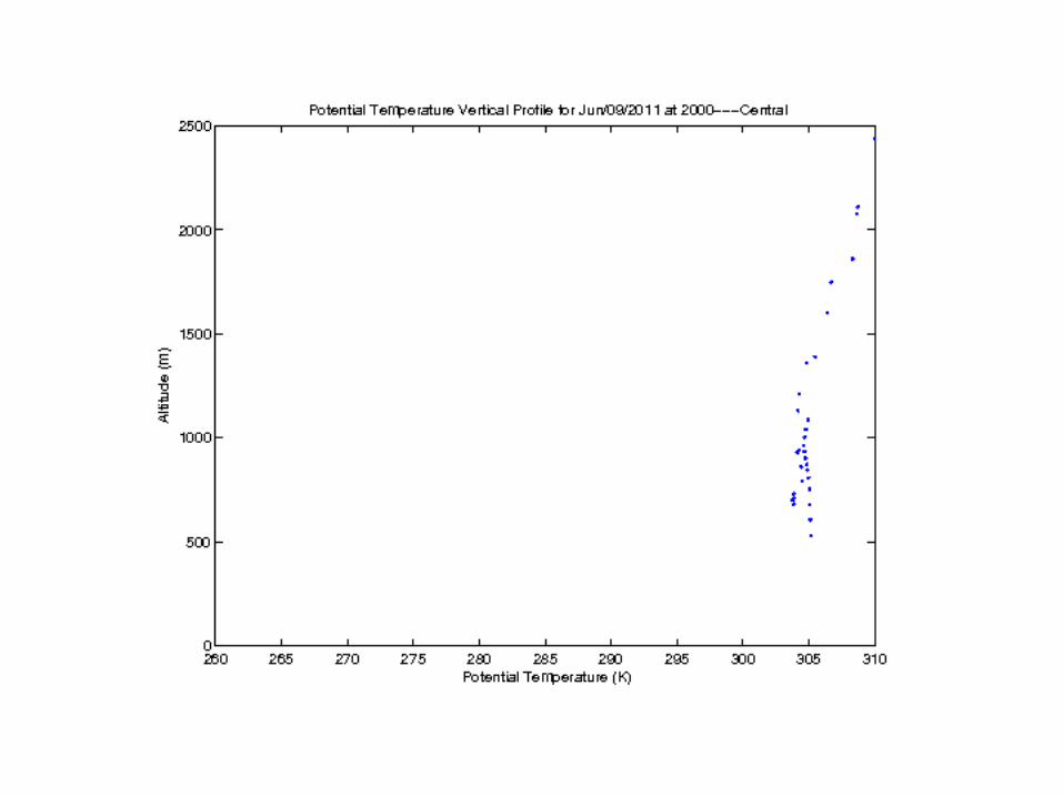
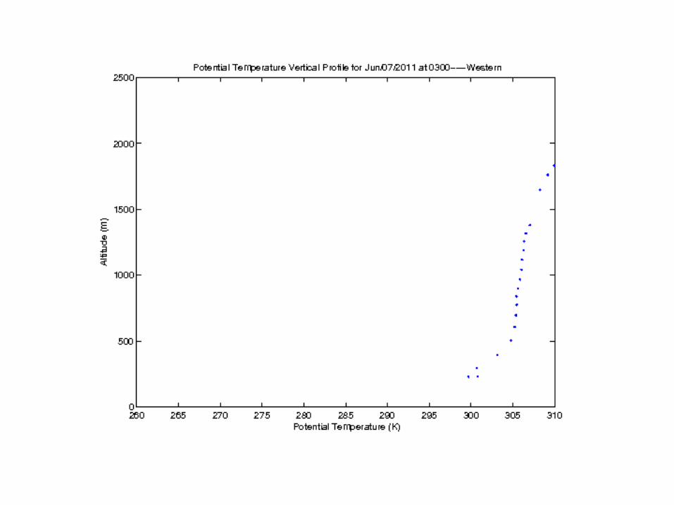
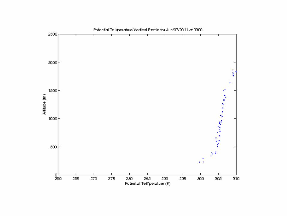
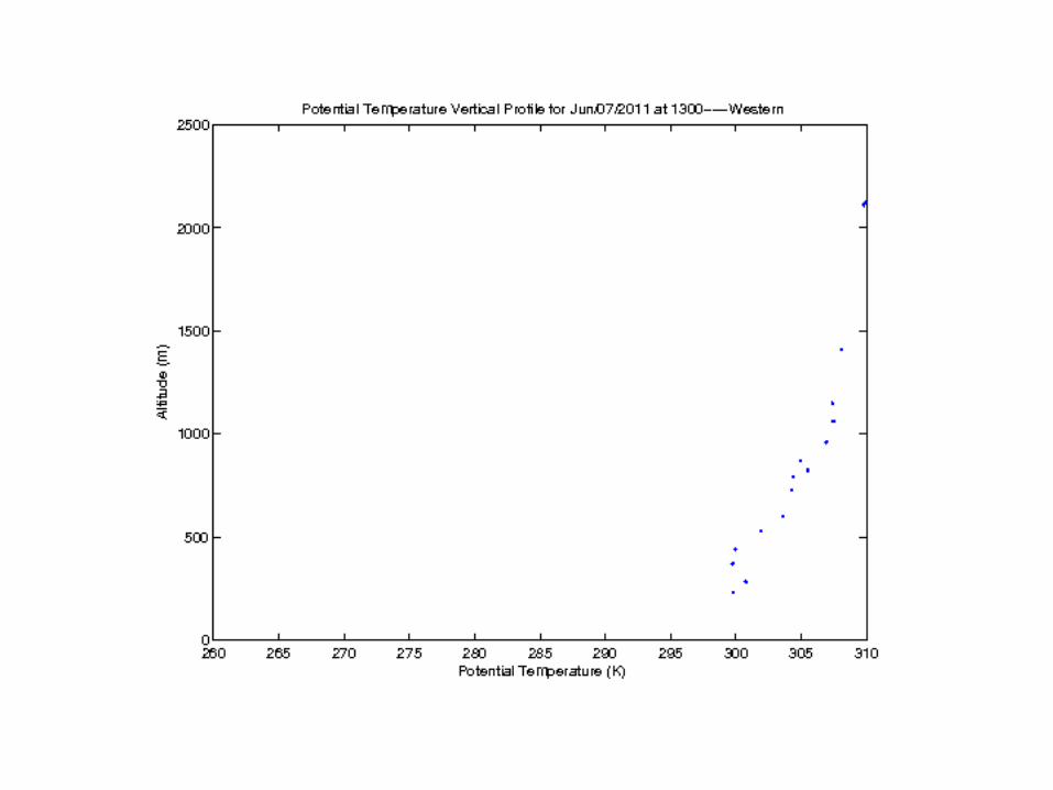
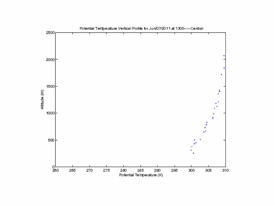
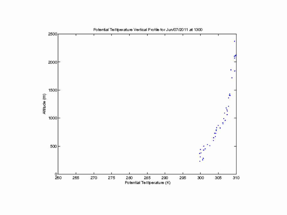
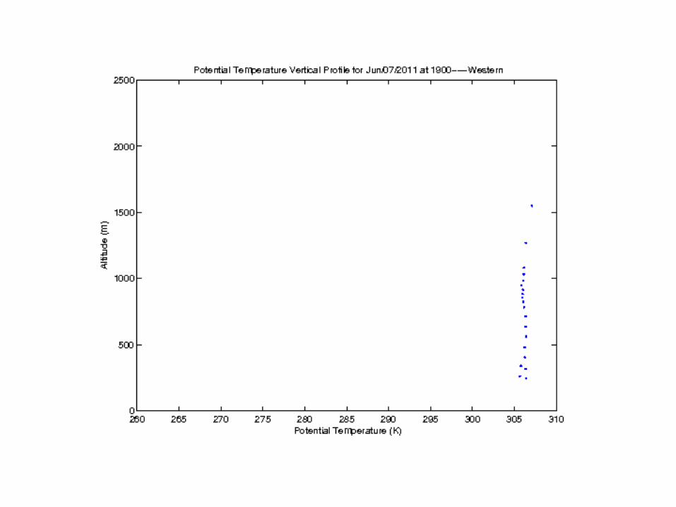
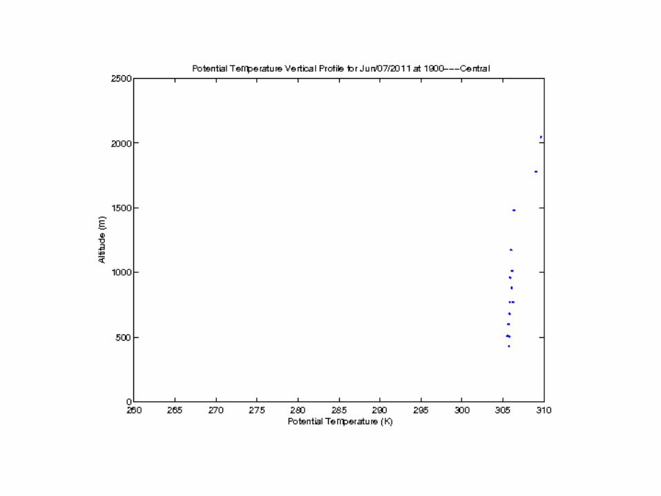
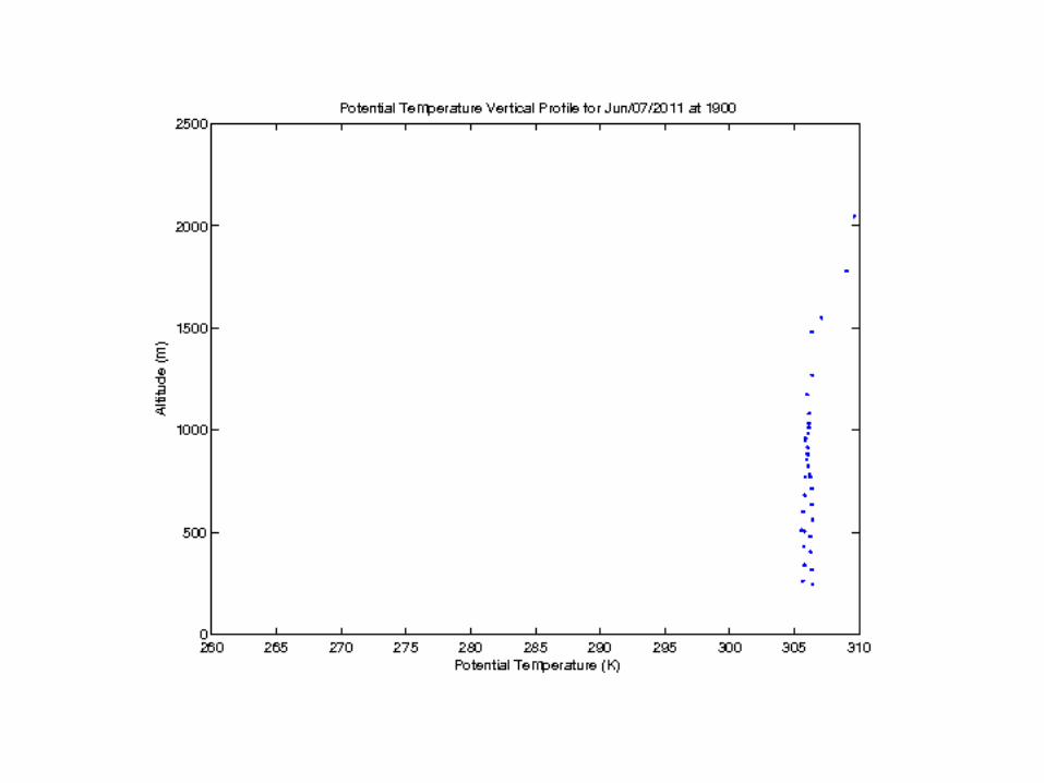
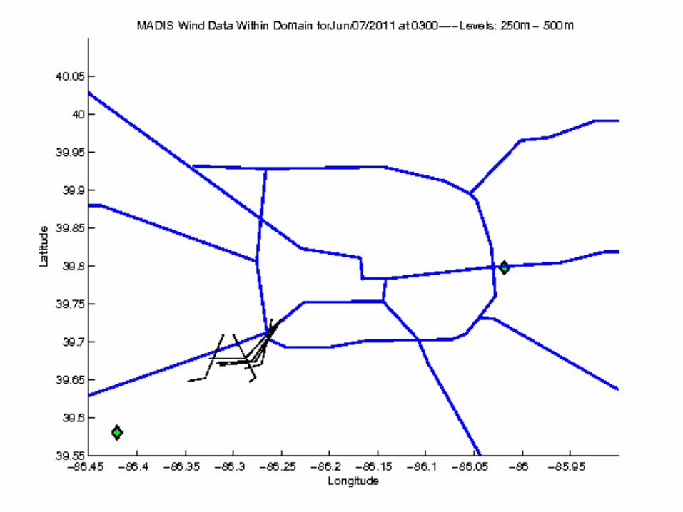
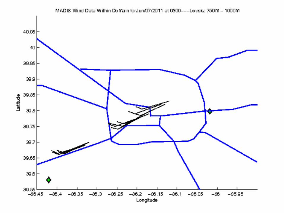
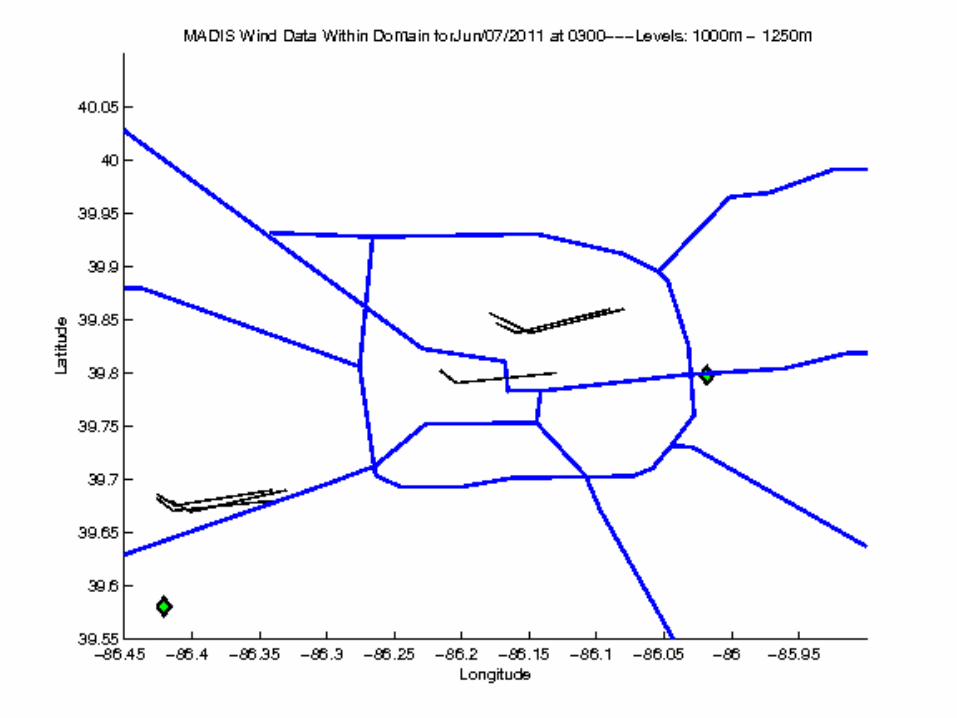
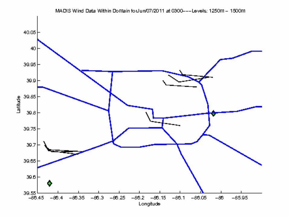
Lesson 6: The city does (not?) significantly alter

the ABL over Indianapolis?

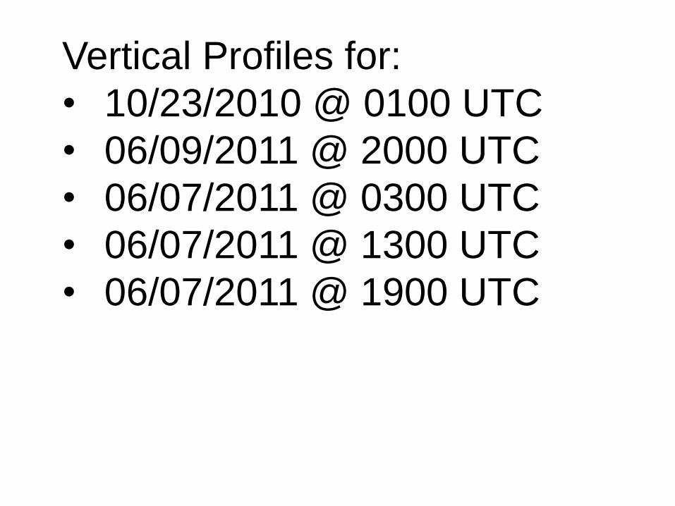
Vertical Profiles for:

• 10/23/2010 @ 0100 UTC

• 06/09/2011 @ 2000 UTC

• 06/07/2011 @ 0300 UTC

• 06/07/2011 @ 1300 UTC

• 06/07/2011 @ 1900 UTC

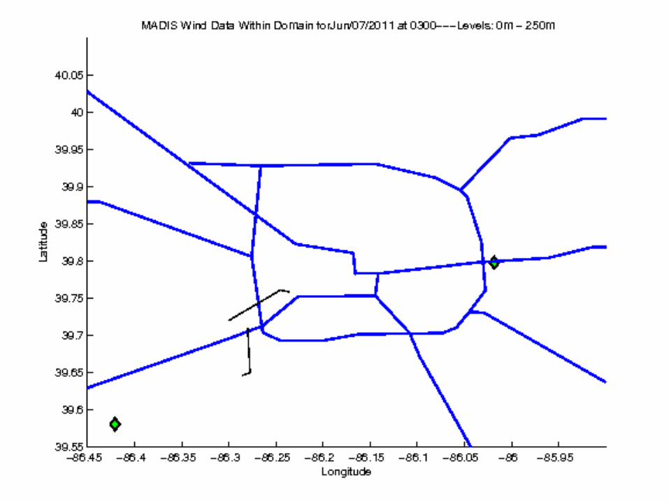
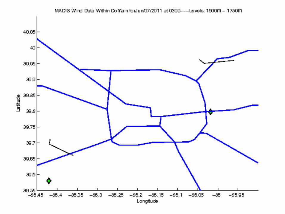
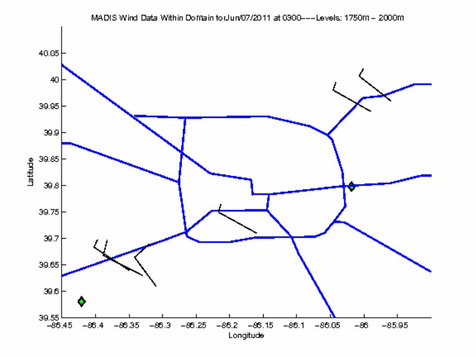
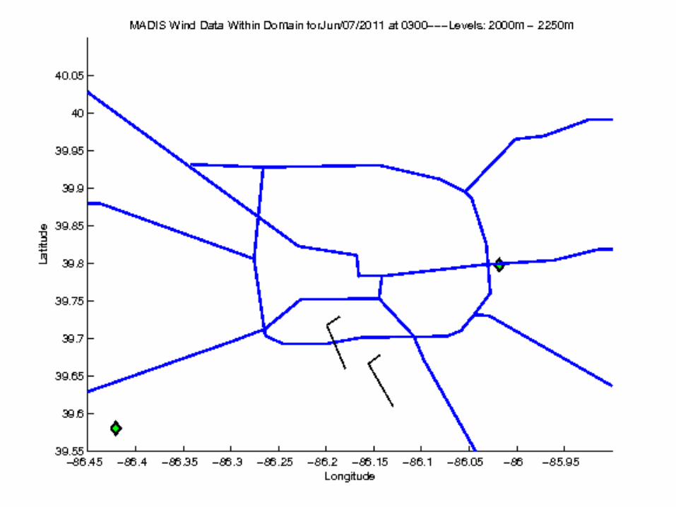
2D Wind Fields – 250m Thick Layers

From Surface to 2500 m

06/07/2011 @ 0300 UTC

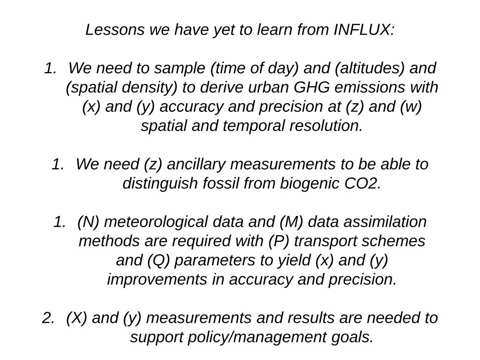
Lessons we have yet to learn from INFLUX:

1. We need to sample (time of day) and (altitudes) and

(spatial density) to derive urban GHG emissions with

(x) and (y) accuracy and precision at (z) and (w)

spatial and temporal resolution.

1. We need (z) ancillary measurements to be able to

distinguish fossil from biogenic CO2.

1. (N) meteorological data and (M) data assimilation

methods are required with (P) transport schemes

and (Q) parameters to yield (x) and (y)

improvements in accuracy and precision.

2. (X) and (y) measurements and results are needed to

support policy/management goals.

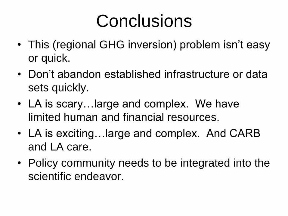
Conclusions

• This (regional GHG inversion) problem isn’t easy

or quick.

• Don’t abandon established infrastructure or data

sets quickly.

• LA is scary…large and complex. We have

limited human and financial resources.

• LA is exciting…large and complex. And CARB

and LA care.

• Policy community needs to be integrated into the

scientific endeavor.

greenhouse gas fluxes derived from regional measurement

Documents