1

Estimating Greenhouse Gas Fluxes From Constructed Wetlands Used

For Water Quality Improvement

Sukanda Chuersuwan1, 2,*

, Pongthep Suwanvaree1, Nares Chuersuwan

3

1 School of Environmental Biology, Institute of Science, Suranaree University of

Technology, Nakhon Ratchasima, Thailand

2Department of Water Resources, Ministry of Natural Resources and Environment,

Samsaen Nai, Phayathai, Bangkok, Thailand

3 School of Environmental Health, Suranaree University of Technology, Nakhon

Ratchasima, Thailand.

Corresponding author, Tel.: 66 44 223927; Fax: 66 44 22 3920.

E-mail addresses: s_lekphet@hotmail.com

Abstract

Methane (CH4), nitrous oxide (N2O) and carbon dioxide (CO2) fluxes were

evaluated from constructed wetlands (CWs) used to improve domestic wastewater quality.

Experiments employed subsurface flow (SF) and free water surface flow (FWS) CWs

planted with Cyperus spp. The results showed seasonal fluctuations of greenhouse gas

fluxes. Greenhouse gas fluxes from SF-CWs and FWS-CWS were significantly different

(p<0.05) while pollutant removal efficiencies of both CWs were not significantly different.

The average CH4, N2O and CO2 fluxes from SF-CWs were 2.9±3.5, 1.0±1.7 and 15.2±12.3

mg/m2/hr, respectively, corresponded to the average global warming potential (GWP) of

392 mg CO2 equivalents/m2/hr. For FWS-CWs, average CH4, N2O and CO2 fluxes were

5.9±4.8, 1.8±1.0 and 29.6±20.2 mg/m2/hr, respectively having the average GWP of 698 mg

2

CO2 equivalents/m2/hr. Thus, FWS-CWs were contributed to higher GWP than SF-CWs

when they were used as a system for domestic water improvement.

Keywords : Greenhouse Gas Fluxes, Methane, Nitrous Oxide, Carbon Dioxide,

Constructed Wetlands, Domestic Wastewater.

1. Introduction

Due in large part to the expectation that climate changes will follow upon an

increase in atmospheric concentration of greenhouse gases (e.g. CO2, CH4, N2O, etc.), there

is intense interest in the sources and sinks of these gases, and in the strength of their

respective emission and consumption. Constructed wetlands (CWs) systems are

combinations of natural wetlands and conventional wastewater treatment processes and are

constructed in order to reduce input of nutrients and organic pollutants to water bodies.

When wetlands are used for purification of wastewater, microbial processes and gas

dynamics are likely to be altered. With increased inputs of nutrients and organic pollutants,

the productivity of the ecosystem could increase as well as the production of greenhouse

gases, which are by- or end-products of microbial decomposition processes. Constructed

wetlands, therefore, can be sources of important greenhouse gases.

There are relatively few studies regarding CH4, N2O and CO2 fluxes emitted from

constructed wetlands used for water quality controlling purposes since the total area of

CWs worldwide is negligible as compare to all natural wetlands and agricultural areas.

However, worldwide increase in the development of CWs necessitates an understanding of

their potential atmospheric impact in light of the trend that natural wetlands in many

3

countries are decreasing (e.g., Thailand) while environmental regulatory agencies are trying

to stimulate an increase in CW acreage. Thus, insight knowledge to clarify the atmospheric

impact of such wetlands is much needed.

CWs gas dynamics are greatly affected by climatic and weather conditions,

especially by temperature and moisture (MacDonald et al., 1998). Rate of photosynthesis

(the source of energy and carbon in ecosystems) and microbial activities producing

greenhouse gases increase with increasing temperature. Both denitrification and methane

formation depend on the oxygen status of the soil or sediment and decomposition rates of

organic matter. As a result, the temporal and seasonal variability of fluxes of CO2, N2O

and CH4 are extremely high resulting from variation in the environmental factors regulating

the microbial processes behind the gas fluxes (Liikanen et al., 2006; Inamori et al., 2007).

In some seasons wetlands can act as a source or sink for carbon and there can be great

differences in the CH4 (Nykánen et al., 1995) and N2O fluxes (Huttunen et al., 2002).

Therefore, prospective studies are needed to obtain a holistic picture of the gas dynamics of

constructed wetlands.

The objectives of this study were: (1) to quantify CH4, N2O and CO2 fluxes from

domestic wastewater treatment constructed wetlands; (2) to estimate seasonal fluctuations

of CH4, N2O and CO2 fluxes from wastewater treatment constructed wetlands; and (3) to

investigate the effect of constructed wetland types on CH4, N2O and CO2 fluxes.

2. Materials and methods

2.1 Study site and constructed wetland systems

4

The experimental scale of constructed wetlands was conducted in four constructed

wetlands (CWs) at 1453’24.48”N and 10200’23.11”E, Suranaree University of

Technology, Nakhon Ratchasima province in the northeastern Thailand. This area of

Thailand has three-season monsoonal climate, with a relatively cool dry season from

November to late February, followed by a hot dry season from March to June and then a

hot rainy season from July to October (TMD, 2011).

The CWs were built based primarily on criteria of aspect ratio (AR) or length to

width of 4:1 to minimize short circuiting and force the flow to move closely to plug flow

hydraulic regime (U.S.EPA, 2000). Each of the units was 2.0 m × 0.5 m × 0.8 m (length ×

width × depth) in dimension. Brick, cement and mortar were the materials used for the

construction of the CWs. Permanent transparent roof made from clear plastic was also

constructed to prevent rain getting into the experiment setup while allowed direct sun light

exposure. Synthetic wastewater similar to domestic discharge from Thailand's Housing

Estates was fed as influent. The compositions of synthetic domestic wastewater consisted

of glucose, FeCl3, NaHCO3, KH2PO4, MgSO47H2O, and urea (Sirianuntapiboon and

Tondee, 2000). Synthetic domestic wastewater was fed daily into the constructed wetlands

containing 17-23 mg/l biochemical oxygen demand (BOD), 115-235 mg/l chemical oxygen

demand (COD), 0.28-0.35 mg/l ammonia nitrogen (NH3-N), and 0.03-0.33 mg/l total

phosphorus (TP). Hydraulic loading rate, the ratio of flow (0.04 m3/d) and surface area (0.5

m x 2.0 m), was estimated to be about 0.04 m/d for each unit. Average organic loading rate

was approximately 42 mg/d.

5

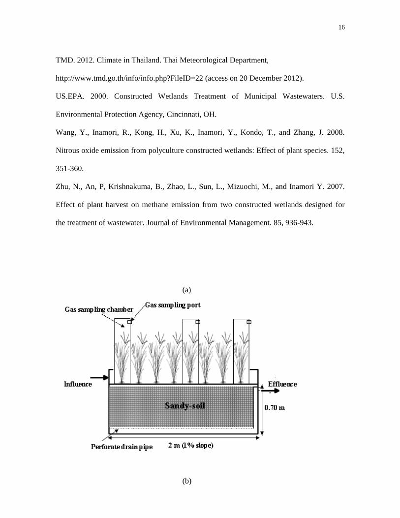
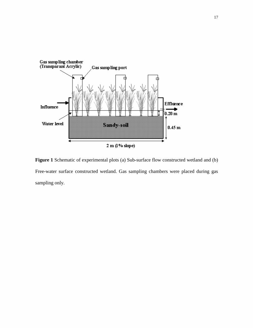
The experiment units were designed to have a duplicate of both sub-surface flow

(SF) beds and free-water surface (FWS) beds. The monoculture emergent plant, Cyperus

spp., was grown in each CW units. The SF constructed wetlands had the media depth of

0.70 m since the water must filtrate down to the bottom and accumulate until it reached the

outlet at 0.65 m. The additional 0.05 m was topsoil. The media depth in FWS constructed

wetlands was approximately 0.45 m in height with the water depth of 0.20 m above the

media, 0.65 m all together (Figure 1).

2.2 Gas fluxes measurement

The gas emissions were measured using a static chamber method described by

Hutchingson and Moiser (1981). The chambers consisted of two parts. The upper part was

constructed from 3.0 mm clear acrylic sheet and made gas-tight by heated glue doubling

with silicon sealant. The acrylic chamber equipped with a thermometer, a fan, and two gas

sampling points. The chamber had a total height of 1.5 m and 0.25 m in width and length

in which the gases emitted from the constructed wetlands were trapped and sampled. A

small fan was operated during the sampling period to create thorough gas mixing inside the

chamber. The lower part was aluminum base to firmly attached acrylic chamber and soil

surface. Four-side groove was made with 4.0 mm trench to accommodate the acrylic

chamber during the gas sampling. The aluminum frame was firmly inserted into the top

soil overnight prior to the measurement. At the beginning, the chamber was placed on top

of the aluminum frame and water was filled in the groove to prevent gas leak. Each

constructed wetlands accommodated three chambers, at the inlet, middle and outlet. Gas

6

measurements were performed at these locations. The sampling periods began at 0, 15, 30

and 45 minute intervals.

Carbon dioxide was measured real-time with CO2 gas analyzer (LI-820 model, LI-

COR, Inc., USA). Data were recorded in computer and retrieved for later analysis. The

instrument used non-dispersive infrared (NDIR) as detector to determine the concentration

of carbon dioxide.

While carbon dioxide was measured real-time in the field, two gas sampling vials

were used to store gas samples. Glass vials were evacuated trapped air inside to generate

negative pressure right before gas sampling. Gas samples were immediately store and kept

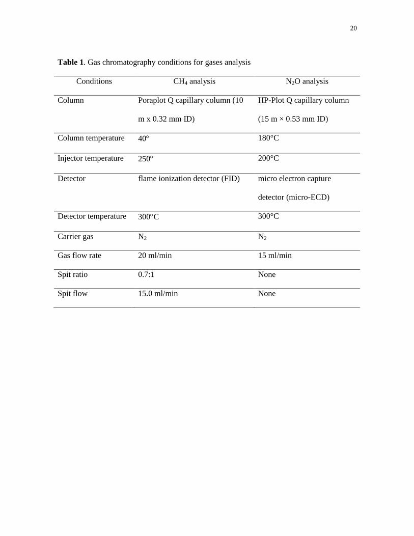
under 4C until the time of analysis. Conditions for gas analysis are listed in Table 1. The

analysis of methane and nitrous oxide were performed with Agilent GC 6890 (Agilent,

USA) equipped with FID and micro-ECD detectors. Agilent Chemstation A.08.03 software

(Agilent, USA) was used for spectrum and determining gas concentrations against standard

gases (Scott Specialty Gases, the Netherlands). The sensitivity of N2O detection was

estimated to be about 0.2 ppmv.

2.3 Gas flux analysis

Emission rates were calculated based on the linear change of gas concentration over

time. The gas concentration for each sample was plotted in a concentration vs. time. The

derivative represents the gas emission rate (ppm/hr) of the series, which were then

converted to flux rates (mg/m2/hr) and corrected for chamber volume and temperature

(Healy et al., 1996). Regressions were performed on each flux rate in Microsoft Excel® to

7

determine linearity of flux. If the increase/decrease in the gas concentration was non-linear

(r2< 0.85) the measurement was rejected (Altor and Mitsch, 2006).

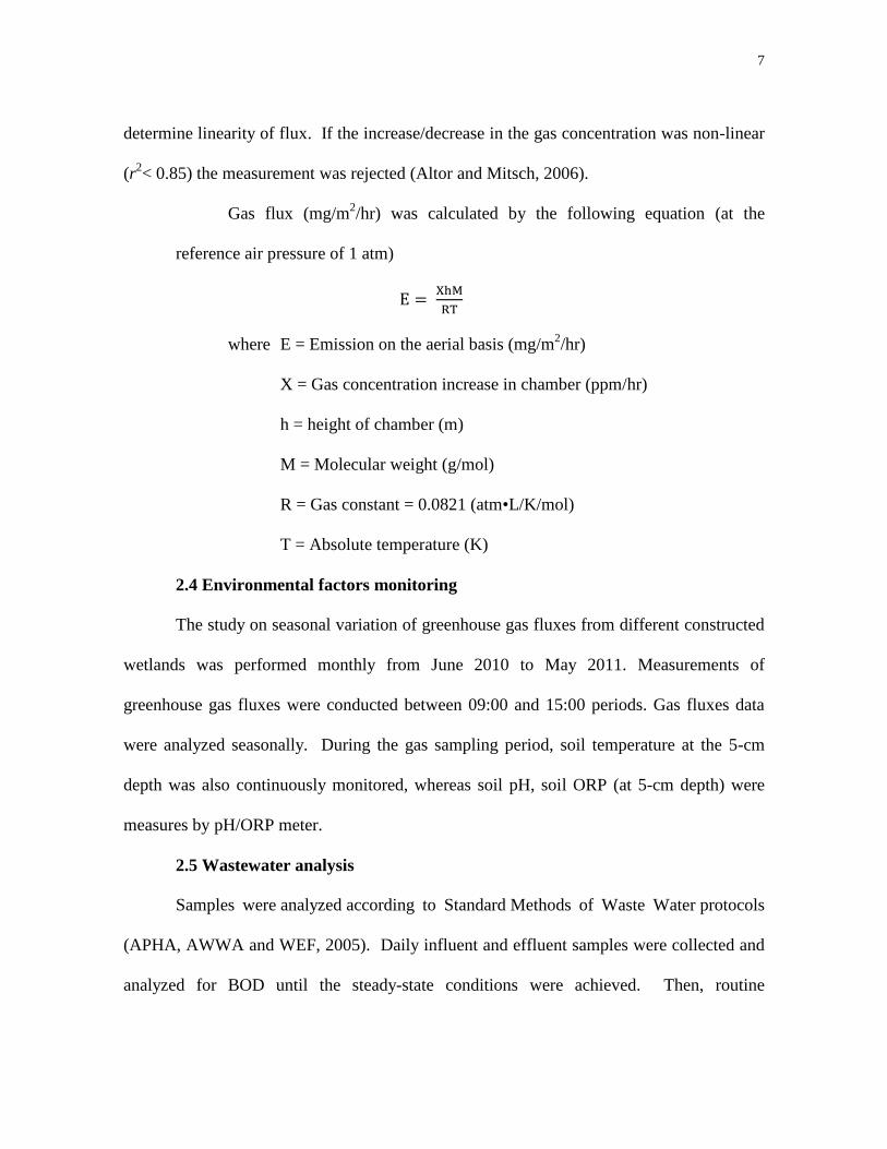
Gas flux (mg/m2/hr) was calculated by the following equation (at the

reference air pressure of 1 atm)

where E = Emission on the aerial basis (mg/m2/hr)

X = Gas concentration increase in chamber (ppm/hr)

h = height of chamber (m)

M = Molecular weight (g/mol)

R = Gas constant = 0.0821 (atm•L/K/mol)

T = Absolute temperature (K)

2.4 Environmental factors monitoring

The study on seasonal variation of greenhouse gas fluxes from different constructed

wetlands was performed monthly from June 2010 to May 2011. Measurements of

greenhouse gas fluxes were conducted between 09:00 and 15:00 periods. Gas fluxes data

were analyzed seasonally. During the gas sampling period, soil temperature at the 5-cm

depth was also continuously monitored, whereas soil pH, soil ORP (at 5-cm depth) were

measures by pH/ORP meter.

2.5 Wastewater analysis

Samples were analyzed according to Standard Methods of Waste Water protocols

(APHA, AWWA and WEF, 2005). Daily influent and effluent samples were collected and

analyzed for BOD until the steady-state conditions were achieved. Then, routine

8

wastewater analysis was carried out to determine the removal efficiency of BOD, COD,

NH3-N, and TP for the period of once a month.

2.6 Data analysis

Statistical analysis was performed with SPSS® and Microsoft Excel

® for Windows

®.

All data entering statistical comparisons were tested for homogeneity of variance and

normal distribution using Levene and Kolmogorov–smirnov Test. If assumptions of normal

distribution were fulfilled, independent–samples t-test was carried out. Otherwise non-

parametric Mann-Whitney U Test was used. All results were considered statistically

significant if p value was <0.05.

3. Results and Discussion

3.1 Performance of pollutant removals

During the operation of constructed wetland units, the removal of BOD, COD, NH3-

N and TP and was investigated, from June 2010 to May 2011. Descriptive statistics for

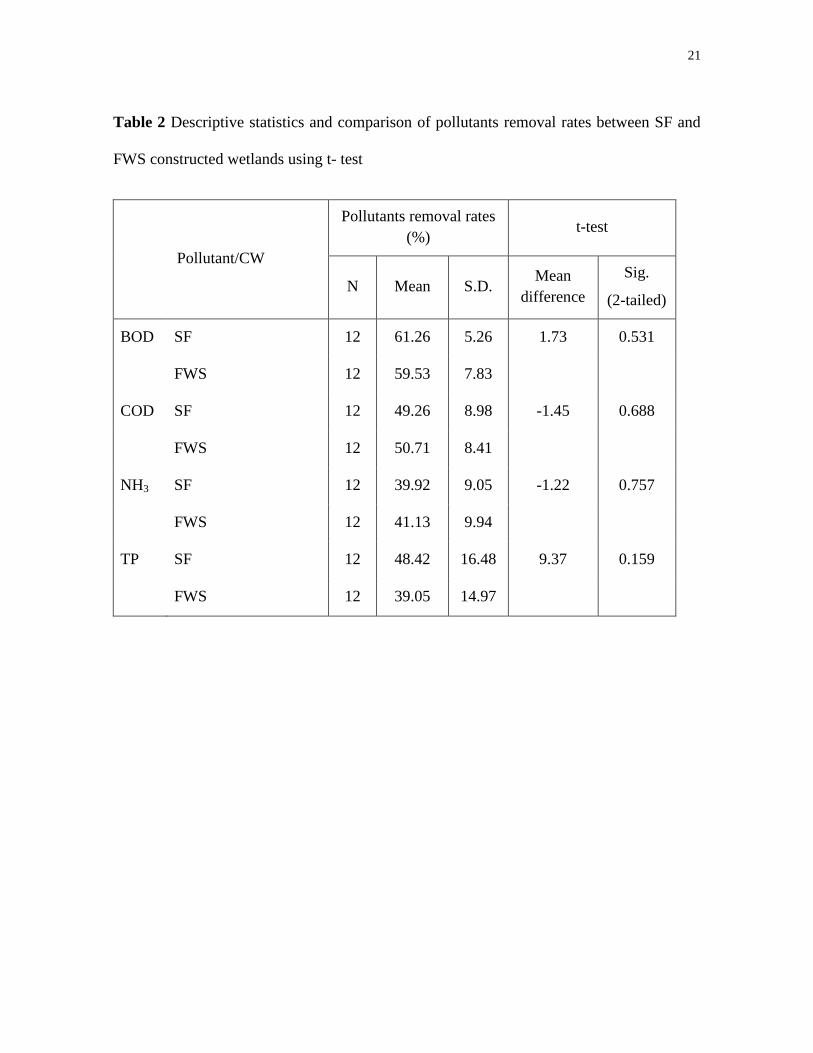
pollutants removal rates of two constructed wetland types are shown in Table 2. Removal

rates of BOD, COD, NH3-N, and TP were in the ranges of 47-69%, 32-65%, 27-60%, and

20-68%, respectively. Since these data were normally distributed and showed homogeneity

of the variances, independent–samples t-test was suitable for the analysis of variation of

pollutants removal rates from different constructed wetlands. Overall performance of

pollutant removals between SF and FWS constructed wetlands showed that pollutant

removal efficiencies of both types constructed wetlands were not significantly different

under experimental conditions. The average removal rates of COD in SF-CW were

comparable to the results reported in Tanzania with the ranged of 33.6%-60.7% (Kaseva,

9

2004) while BOD removal rates was a bit lower than the results reported by Hadad et al.,

(2006) in Argentina at 76%. The highest removal rate of TP in this present study was

similar to Hadad et al., (2006) as well.

3.2 Seasonal variations of greenhouse gas fluxes and environmental factors

3.2.1 Seasonal variations of methane fluxes from constructed wetlands

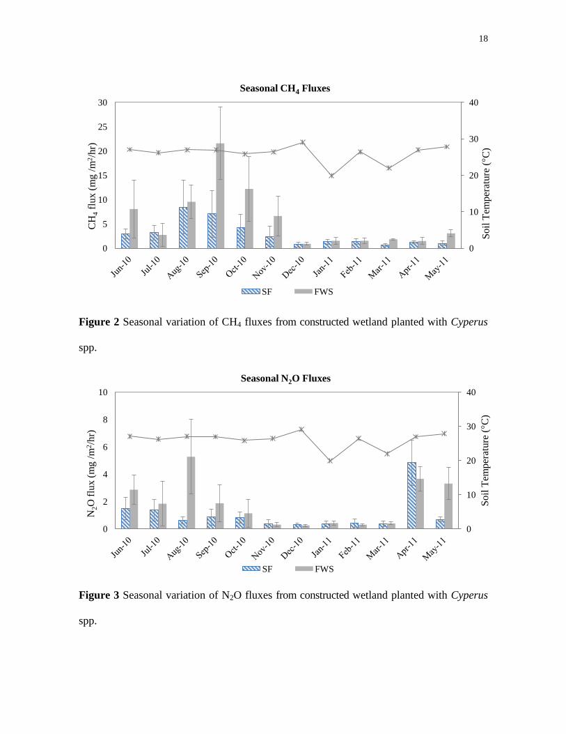
During one year of experiment, CH4 fluxes from all constructed wetlands were

noticeable higher in August and November than those in other months (Figure 2). The

highest CH4 fluxes from SF occurred in August with the average of 10.5 mg/m2/hr whereas

FWS occurred in October with the average of 15.3 mg/m2/hr. The lowest CH4 fluxes from

SF occurred in May with the average of 0.7 mg/m2/hr whereas FWS occurred in December

with the average of 1.0 mg/m2/hr. When seasonal variation was taken into account, the

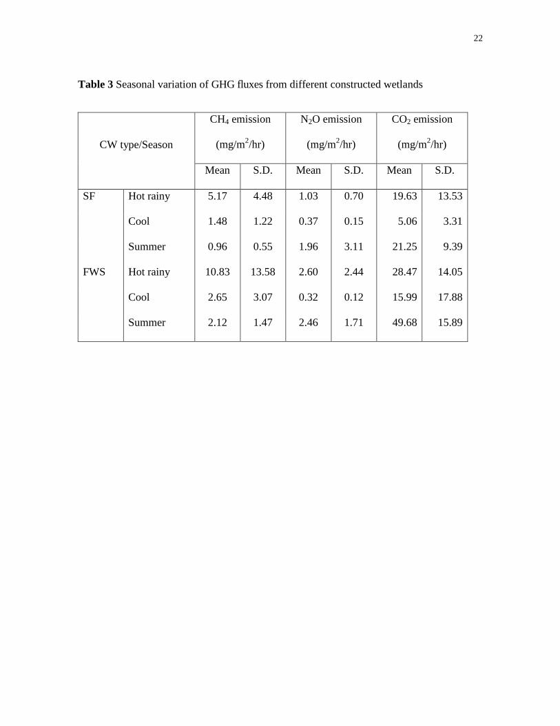
results showed that CH4 fluxes from SF and FWS constructed wetlands were highest in hot

rainy season (July - October) with the average of 5.2 and 10.8 mg/m2/hr, respectively,

followed by cold season (November-February) with the average of 1.5 and 2.6 mg/m2/hr,

respectively, and lowest in summer season (March-June) with the average of 1.0 and 2.1

mg/m2/hr, respectively. Environmental parameters monitored during the experiment

showed an unusual phenomenon in the area especially air temperature at the end of 2010

and early 2011. Monthly average of air temperature reached maximum in September

(36.7C) while the lowest mean was found in March (24.7C). It is important to note that

the lower air temperature in March was quite unusual but it occurred in March 2011. Soil

temperatures, measured at 5 cm depth, were in the optimum range for microbial activities

and changed in a narrow-range during three seasons. It peaked in December (29C) with

10

average of 29C and reached its minimum value in January (19.9C) before it rise again in

summer season (March-June).

3.2.2 Seasonal variations of nitrous oxide fluxes from constructed wetlands

N2O fluxes were high during April and October compared with the rest of the year

(Figure 3). The highest N2O fluxes from SF occurred in April with the average of 5.3

mg/m2/hr whereas FWS occurred in August with the average of 6.9 mg/m

2/hr. The lowest

N2O fluxes from SF occurred in January with the average of 0.3 mg/m2/hr whereas FWS

occurred in December with the average of 0.3 mg/m2/hr. When seasonal variation was

taken into account, N2O fluxes from SF was highest in summer season (March-June) with

the average of 2.0 mg/m2/hr, followed by hot rainy season (July-October) with the average

of 1.0 mg/m2/hr, and lowest in cold season (November-February) with the average of 0.4

mg/m2/hr. While N2O fluxes from FWS was highest in hot rainy season (July-October)

with average of 2.6 mg/m2/hr, followed by summer season (March–June) with average of

2.5 mg/m2/hr and lowest in cold season (November-February) with average of 0.3

mg/m2/hr.

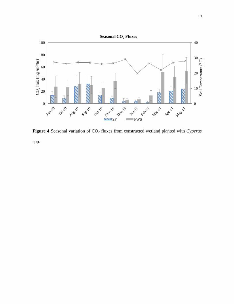
3.2.3 Seasonal variations of carbon dioxide fluxes from constructed wetlands

Estimated CO2 fluxes were low in December and February. The highest CO2 fluxes

from SF occurred in September with the average of 32.7 mg/m2/hr whereas FWS occurred

in May with the average of 60.2 mg/m2/hr (Figure 4). The lowest CO2 fluxes from SF

occurred in February with the average of 3.2 mg/m2/hr whereas FWS occurred in December

with the average of 8.5 mg/m2/hr. In the case of seasonal variations, CO2 fluxes from SF

and FWS were highest in summer season (March-June) with average of 21.2 and 49.7

11

mg/m2/hr, respectively, followed by hot rainy season (July-October) with average of 19.6

and 28.5 mg/m2/hr, respectively, and lowest in cool season (November-February) with

average of 5.1 and 15.6 mg/m2/hr, respectively.

GHG fluxes from CWs were observed but the pattern of seasonal CO2 variations

and environmental factors was not distinct. It was possible that important environmental

factors such as soil temperature, soil pH, and soil ORP were in the optimum range for GHG

production and changed occurred in a narrow-range during the experiment. Another reason

was that GHG fluxes were not the result of a one-factor action but of the interaction of

more biotic and abiotic factors. Soil pH was in the range of 6.70 to 8.02, and soil ORP was

in negative range (-168 to -232 mV). In cold climate, SØvic and KlØve (2007) reported

seasonal variations differences of N2O from FWS-CWs in which N2O emissions were

highest in autumn while CH4 did not show significant seasonal difference.

3.3 Greenhouse gas fluxes and constructed wetland type

The investigation of GHG fluxes from different type of constructed wetlands found

that CH4, N2O and CO2 fluxes released from SF-CWs had the average of 2.9±2.5, 1.0±0.7

15.2±12.3 mg/m2/hr, respectively. In FWS-CWs, CH4, N2O and CO2 fluxes had the

average of 5.9±4.8, 1.8±1.0 and 29.6±20.2 mg/m2/hr, respectively. Kaewkamthong (2002)

reported the flux of CH4 from FWS-CWs planted with Digitaria bicornis and Typha

angustifolia in the range of 2.7 – 75.7 mg/m2/hr. In Japan, Zhu et al., (2007) used

Phargmites communit in FWS-CWs and CH4 flux varied from 0-4 mg/m2/hr. Estimated

N2O flux from SF-CWs in another experiment in Japan was 0-1.4 mg/m2/hr (Wang et al.,

2008). Mander et al., (2008) reported the range of CH4 and N2O fluxes from FWS-CWs

12

used in Estonia to be about 0.06-0.17 and 0.05-0.06 mg/m2/hr, respectively. Our results

were in the range reported in hot climate but somewhat higher than the values found in

European studies. However, the effect of different plants on GHGs fluxes remains debated

(Maltais-Landry et al., 2009).

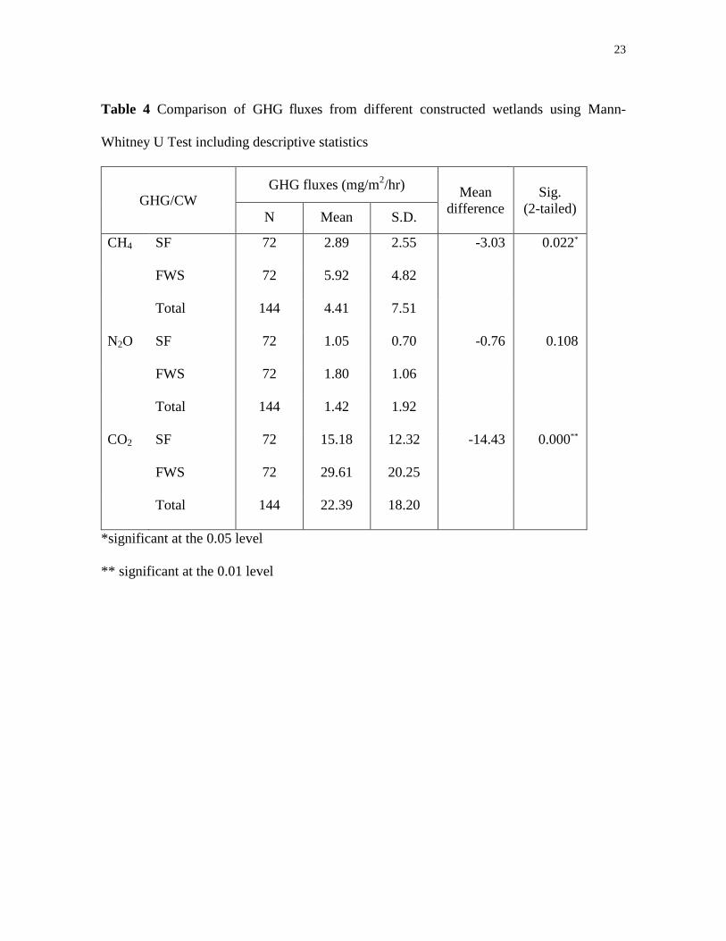
When compare the results from SF-CWs and FWS-CWs, CH4 and CO2 fluxes were

significantly different (p<0.05) (Table 4). Average CH4 and CO2 fluxes from FWS-CWs

were significantly higher than the fluxes from SF-CWs. However, there was no

significantly different (p>0.05) in average N2O fluxes from SF and FWS constructed

wetlands.

3.4 Global warming potential of greenhouse gases from SF and FWS

constructed wetlands

Due to differences in potential to cause global warming, it was important to estimate

the impact of greenhouse gases in terms of global warming potential (GWP) described by

IPCC (2001). The average GWP of CH4 and N2O were 23 and 296 times of CO2,

respectively. In the present study, estimated GWP of SF-CWs was about 66 and 311 mg

CO2 equivalents/m2/hr for CH4 and N2O, respectively. Overall, the greenhouse gas flux

from SF-CWs was approximately 392 mg CO2 equivalents/m2/hr. Estimated GWP of

FWS-CWs was about 136 and 533 mg CO2 equivalents/m2/hr for CH4 and N2O,

respectively. Combined GWP of all greenhouse gases was approximately 698 mg CO2

equivalents/m2/hr. Thus, the results indicated that the estimated GWP of GHG fluxes from

FWS-CWs was higher than SF-CWs about 1.8 times. It indicated that the FWS-CWs

planted with Cyperus spp. has higher potential in response to global warming compared to

SF-CWs when they were used to improve water quality.

13

4. Conclusions

The average CH4, N2O and CO2 fluxes from SF-CWs planted with Cyperus spp.,

were 2.9±2.5, 1.05±0.7 and 15.2±12.3 mg/m2/hr, respectively. Higher flux was found from

FWS-CWs with the average of CH4, N2O and CO2 fluxes at 5.9±4.8, 1.8±1.0 and 29.6±20.2

mg/m2/hr, respectively. Seasonal fluctuations of GHG fluxes from wastewater treatment

constructed wetlands could be observed. However, the pattern of seasonal CO2 variations

and environmental factors was not distinct.

GHG fluxes from SF and FWS constructed wetland showed significantly different

(p<0.05) while pollutant removal efficiencies of both constructed wetlands were not

significantly different. The average GWP of SF-CWs and FWS-CWs were approximately

392 and 698 mg CO2 equivalents/m2/hr, respectively. Thus, GWP released for FWS was

higher than SF constructed wetlands.

For better understanding about GHG fluxes from constructed wetlands, further

study should be conducted on influencing factors related to the rate of GHG production,

entrapment, oxidation and emission. Additionally, GHG fluxes from constructed wetlands

may be influenced by other factors, such as type and amount of substrates, water chemistry

(e.g. dissolved SO4-2

or NO3-) and the activity of microorganism.

5. Acknowledgement

This study was supported by Environmental Biology Program, Institute of Sciences,

Suranaree University of Technology. The authors gratefully acknowledge the support.

6. References

14

Altor, A.E., and Mitsch, W.J., 2006. Methane flux from created riparian marshes:

Relationship to intermittent vs. continuous inundation and emergent macrophytes.

Ecological Engineering, 28, 224–234.

APHA-AWWA-WEF. 2005. Standard Methods for The Examination of Water and

Wastewater, 21st edition. American Public Health Association, Washington, DC.

Hadad, H.R., Maine, M.A., and Bonetto, C.A. 2006. Macrophyte growth in a pilot-scale

constructed wetland for industrial wastewater treatment. Chemosphere. 63, 1744-1753.

Healy, M.G., Devine, C.M. and Murphy, R., 1996. Microbial production of biosurfactants.

Resources, Conservation and Recycling, 18, 41-57.

Hutchinson, G. L., Mosier, A, R., 1981. Improved soil cover method for field measurement

of nitrous oxide fluxes. Soil Science Society of America Journal.45, 311–316.

Huttunen, J.T., Väisänen, T.S., Hellsten, S.K., Heikkinen, M., Nykänen, H., Jungner, H.,

Niskanen, A., Virtanen, M.O., Lindqvist, O.V., Nenonen, O., and Martikainen, P.J., 2002.

Fluxes of CH4, CO2, and N2O in hydroelectric reservoirs Lokka and Porttipahta in the

northern boreal zone in Finland. Global Biogeochemical Cycles, 16(1): 1003

doi:10.1029/2000GB001316.

Inamori, R., Gui, P., Dass, P., Matsumura, M., Xu, K-Q., Kondo, T., Ebie, Y., and Inamori,

Y., 2007. Investigating CH4 and N2O emissions from eco-engineering wastewater

treatment processes using constructed wetland microcosms. Process Biochemistry. 42,

363-373.

Kaewkamthong, N. 2002. Methane emission from constructed wetland. Master Thesis,

King Mongkut’s University of Technology, Bangkok, Thailand.

15

Kaseva, M.E. 2004. Performance of a sub-surface flow constructed wetland in polishing

pre-treated wastewater-a tropical case study. Water Research. 38, 681-687.

Liikanen, A., Huttunen, J.T., Karjalainen, S.M., Heikkinen K., Tero S. V¨ais¨anen, T.S.,

Nyk¨anen, H., and Martikainen, P.J., 2006. Temporal and seasonal changes in greenhouse

gas emissions from a constructed wetland purifying peat mining runoff waters. Ecological

Engineering. 26, 241-251.

MacDonald, J.A., Fowler, D., Hargreaves, K.J., Skiba, U., Leith, I.D., and Murray, M.B.,

1998. Methane emission rates from a northern wetland; response to temperature, water

table and transport. Atmospheric Environment. 32, 3219–3227.

Maltais-Landry, G., Maranger, R., Brisson, J., and Chazarenc F. 2009. Greenhouse gas

production and efficiency of planted and artificially aerated constructed wetlands.

Environmental Pollution. 157, 748-754.

Mander, Ü., Lõhmus, K., Teiter, S., Mauring, T., Nurk, K., and Augustin, J. 2008. Gaseous

fluxes in the nitrogen and carbon budgets of subsurface flow constructed wetlands. Science

of the Total Environment. 404, 343-353.

Nykánen, H., Alm, J., L°ang, K., Silvola, J., and Martikainen, P.J., 1995. Emissions of

CH4, N2O and CO2 from a virgin fen and a fen drained for grassland in Finland. Journal of

Biogeography. 22, 351–357.

Sirianuntapiboon, S. and Tondee, T., 2000. Application of packed cage RBC system for

treating wastewater contaminated with nitrogenous compounds. Thammasat International

Journal of Science and Technology. 5(1), 28–39.

SØvik, A.K., and KlØve, B. 2007. Emission of N2O and CH4 from a constructed wetland in

southeastern Norway. Science of the Total Environment. 380(28-37).

16

TMD. 2012. Climate in Thailand. Thai Meteorological Department,

http://www.tmd.go.th/info/info.php?FileID=22 (access on 20 December 2012).

US.EPA. 2000. Constructed Wetlands Treatment of Municipal Wastewaters. U.S.

Environmental Protection Agency, Cincinnati, OH.

Wang, Y., Inamori, R., Kong, H., Xu, K., Inamori, Y., Kondo, T., and Zhang, J. 2008.

Nitrous oxide emission from polyculture constructed wetlands: Effect of plant species. 152,

351-360.

Zhu, N., An, P, Krishnakuma, B., Zhao, L., Sun, L., Mizuochi, M., and Inamori Y. 2007.

Effect of plant harvest on methane emission from two constructed wetlands designed for

the treatment of wastewater. Journal of Environmental Management. 85, 936-943.

(a)

(b)

17

Figure 1 Schematic of experimental plots (a) Sub-surface flow constructed wetland and (b)

Free-water surface constructed wetland. Gas sampling chambers were placed during gas

sampling only.

18

Figure 2 Seasonal variation of CH4 fluxes from constructed wetland planted with Cyperus

spp.

Figure 3 Seasonal variation of N2O fluxes from constructed wetland planted with Cyperus

spp.

0

10

20

30

40

0

5

10

15

20

25

30

So

il T

emp

erat

ure

(°C

)

CH

4 f

lux

(m

g /

m2/h

r)

Seasonal CH4 Fluxes

SF FWS

0

10

20

30

40

0

2

4

6

8

10

Soil

Tem

per

ature

(°C

)

N2O

flu

x (

mg /

m2/h

r)

Seasonal N2O Fluxes

SF FWS

19

Figure 4 Seasonal variation of CO2 fluxes from constructed wetland planted with Cyperus

spp.

0

10

20

30

40

0

20

40

60

80

100

So

il T

emp

erat

ure

(°C

)

CO

2 f

lux

(m

g /

m2/h

r)

Seasonal CO2 Fluxes

SF FWS

20

Table 1. Gas chromatography conditions for gases analysis

Conditions CH4 analysis N2O analysis

Column Poraplot Q capillary column (10

m x 0.32 mm ID)

HP-Plot Q capillary column

(15 m × 0.53 mm ID)

Column temperature 40 180°C

Injector temperature 250 200°C

Detector flame ionization detector (FID) micro electron capture

detector (micro-ECD)

Detector temperature 300C 300°C

Carrier gas N2 N2

Gas flow rate 20 ml/min 15 ml/min

Spit ratio 0.7:1 None

Spit flow 15.0 ml/min None

21

Table 2 Descriptive statistics and comparison of pollutants removal rates between SF and

FWS constructed wetlands using t- test

Pollutant/CW

Pollutants removal rates

(%) t-test

N Mean S.D. Mean

difference

Sig.

(2-tailed)

BOD SF 12 61.26 5.26 1.73 0.531

FWS 12 59.53 7.83

COD SF 12 49.26 8.98 -1.45 0.688

FWS 12 50.71 8.41

NH3 SF 12 39.92 9.05 -1.22 0.757

FWS 12 41.13 9.94

TP SF 12 48.42 16.48 9.37 0.159

FWS 12 39.05 14.97

22

Table 3 Seasonal variation of GHG fluxes from different constructed wetlands

CW type/Season

CH4 emission

(mg/m2/hr)

N2O emission

(mg/m2/hr)

CO2 emission

(mg/m2/hr)

Mean S.D. Mean S.D. Mean S.D.

SF Hot rainy 5.17 4.48 1.03 0.70 19.63 13.53

Cool 1.48 1.22 0.37 0.15 5.06 3.31

Summer 0.96 0.55 1.96 3.11 21.25 9.39

FWS Hot rainy 10.83 13.58 2.60 2.44 28.47 14.05

Cool 2.65 3.07 0.32 0.12 15.99 17.88

Summer 2.12 1.47 2.46 1.71 49.68 15.89

23

Table 4 Comparison of GHG fluxes from different constructed wetlands using Mann-

Whitney U Test including descriptive statistics

GHG/CW GHG fluxes (mg/m

2/hr)

Mean

difference

Sig.

(2-tailed) N Mean S.D.

CH4 SF 72 2.89 2.55 -3.03 0.022*

FWS 72 5.92 4.82

Total 144 4.41 7.51

N2O SF 72 1.05 0.70 -0.76 0.108

FWS 72 1.80 1.06

Total 144 1.42 1.92

CO2 SF 72 15.18 12.32 -14.43 0.000**

FWS 72 29.61 20.25

Total 144 22.39 18.20

*significant at the 0.05 level

** significant at the 0.01 level