Greedy Algorithms for Steiner Forest

Anupam Gupta∗ Amit Kumar†

Abstract

In the Steiner Forest problem, we are given terminal pairs si, ti, and need to find the cheapestsubgraph which connects each of the terminal pairs together. In 1991, Agrawal, Klein, and Ravi,and Goemans and Williamson gave primal-dual constant-factor approximation algorithms for thisproblem; until now the only constant-factor approximations we know are via linear programmingrelaxations.

In this paper, we consider the following greedy algorithm:

Given terminal pairs in a metric space, a terminal is active if its distance to its partneris non-zero. Pick the two closest active terminals (say si, tj), set the distance betweenthem to zero, and buy a path connecting them. Recompute the metric, and repeat.

It has long been open to analyze this greedy algorithm. Our main result: this algorithm is aconstant-factor approximation.

We use this algorithm to give new, simpler constructions of cost-sharing schemes for Steiner forest.In particular, the first “strict” cost-shares for this problem implies a very simple combinatorialsampling-based algorithm for stochastic Steiner forest.

∗Computer Science Department, Carnegie Mellon University, Pittsburgh, PA 15213, USA. Research partly supportedby NSF awards CCF-1016799 and CCF-1319811.†Dept. of Computer Science and Engg., IIT Delhi, India 110016.

arX

iv:1

412.

7693

v1 [

cs.D

S] 2

4 D

ec 2

014

1 Introduction

In the Steiner forest problem, given a metric space and a set of source-sink pairs si, tiKi=1, a feasiblesolution is a forest such that each source-sink pair lies in the same tree in this forest. The goal isto minimize the cost, i.e., the total length of edges in the forest. This problem is a generalizationof the Steiner tree problem, and hence APX-hard. The constant-factor approximation algorithmscurrently known for it are all based on linear programming techniques. The first such result was aninfluential primal-dual 2-approximation due to Agrawal, Klein, and Ravi [AKR95]; this was simplifiedby Goemans and Williamson [GW95] and extended to many “constrained forest” network designproblems. Other works have since analyzed the integrality gaps of the natural linear program, andfor some stronger LPs; see § 1.2.

However, no constant-factor approximations are known based on “purely combinatorial” techniques.Some natural algorithms have been proposed, but these have defied analysis for the most part. Thesimplest is the paired greedy algorithm that repeatedly connects the yet-unconnected si-ti pair at min-imum mutual distance; this is no better than Ω(log n) (see Chan, Roughgarden, and Valiant [CRV10]or Appendix A). Even greedier is the so-called gluttonous algorithm that connects the closest twoyet-unsatisfied terminals regardless of whether they were “mates”. The performance of this algorithmhas been a long-standing open question. Our main result settles this question.

Theorem 1.1 The gluttonous algorithm is a constant-factor approximation for Steiner Forest.

We then apply this result to obtain a simple combinatorial approximation algorithm for the two-stage stochastic version of the Steiner forest problem. In this problem, we are given a probabilitydistribution π defined over subsets of demands. In the first stage, we can buy some set E1 of edges.Then in the second stage, the demand set is revealed (drawn from π), and we can extend the set E1 toa feasible solution for this demand set. However, these edges now cost σ > 1 times more than in thefirst stage. The goal is to minimize the total expected cost. It suffices to specify the set E1—once theactual demands are known, we can augment using our favorite approximation algorithm for Steinerforest. Our simple algorithm is the following: sample dσe times from the distribution π, and let E1

be the Steiner forest constructed by (a slight variant of) the gluttonous algorithm on union of thesedσe demand sets sampled from π.

Theorem 1.2 There is a combinatorial (greedy) constant-factor approximation algorithm for thestochastic Steiner forest problem.

Showing that such a “boosted sampling” algorithm obtained a constant factor approximation hadproved elusive for several years now; the only constant-factor approximation for stochastic Steinerforest was a complicated primal-dual algorithm with a worse approximation factor [GK09]. Ourresult is based on the first cost sharing scheme for the Steiner forest problem which is constant strictwith respect to a constant factor approximation algorithm; see § 5 for the formal definition. Such acost sharing scheme can be used for designing approximation algorithms for several stochastic networkdesign problems for the Steiner forest problem. In particular, we obtain the following results:

• For multi-stage stochastic optimization problem for Steiner forest, our strict-cost sharing schemealong with the fact that it is also cross-monotone implies the first O(1)k-approximation algo-rithm, where k denotes the number of stages (see [GPRS11] for formal definitions and the relationwith cost sharing).

• Consider the online stochastic problem, where given a set of source-sink pairs D in a metricM, and a probability distribution π over subsets of D (i.e., over 2D), an adversary choosesa parameter k, and draws k times independently from π. The on-line algorithm, which can

1

sample from π, needs to maintain a feasible solution over the set of demand pairs produced bythe adversary at all time. The goal is to minimize the expected cost of the solution produced bythe algorithm, where the expectation is over π and random coin tosses of the algorithm. Our costsharing framework gives the first constant competitive algorithm for this problem, generalizingthe result of Garg et al. [GGLS08] which works for the special case when π is a distribution overD (i.e., singleton subsets of D).

1.1 Ideas and Techniques

We first describe the gluttonous algorithm. Call a terminal active if it is not yet connected to itsmate. Recall: our algorithm merges the two active terminals that are closest in the current metric(and hence zeroes out their distance). At any point of time, we have a collection of supernodes, eachsupernode corresponding to the set of terminals which have been merged together. A supernode isactive if it contains at least one active terminal. Hence the algorithm can be alternatively describedthus: merge the two active supernodes that are closest (in the current metric) into a new supernode.(A formal description of the algorithm appears in §2.)

The analysis has two conceptual steps. In the first step, we reduce the problem to the special casewhen the optimal solution can be (morally) assumed to be a single tree (formally, we reduce to thecase where the gluttonous’ solution is a refinement of the optimal solution). The proof for this partis simple: we take an optimal forest, and show that we can connect two trees in the forest if thegluttonous algorithm connects two terminals lying in these two trees, incurring only a factor-of-twoloss.

u

a

b

cv

d

Figure 1.1: Example showingthe construction of tree T ′ from T ,which is shown in solid lines. If wemerge u and u′, we can remove theedge (a, b) to get the tree T ′. As-suming a is not active, we can alsoshort-cut the degree 2 vertex a inT ′ by replacing the edges (s, a) and(a, d) with the edge (s, d).

The second step of the analysis starts with the tree solution Tpromised by the first step of the analysis. As the gluttonous algo-rithm proceeds, the analysis alters T to maintain a candidate solu-tion to the current set of supernodes. E.g., if we merge two activesupernodes u and v to get a new supernode uv. We want to alterthe solution T on the original supernodes to get a new solution T ′,say by removing an edge from the (unique) u-v path in T , and thenshort-cutting any degree two inactive supernode in T ′ (see Figure 1.1for an example). The hope is to argue that the distance between uand v—which is the cost incurred by gluttonous—is commensurateto the cost of the edge of T which gets removed during this process.This would be easy if there were a long edge on u-v path in the treeT . The problem: this may not hold for every pair of supernodes wemerge. Despite this, our analysis shows that the bad cases cannothappen too often, and so we can perform this charging argument inan amortized sense.

Our analysis is flexible and extends to other variants of the gluttonousalgorithm. A natural variant is one where, instead of merging the twoclosest active supernodes, we contract the edges on a shortest path between the two closest activesupernodes. The first step of the above analysis does not hold any more. However, we show that itis enough to account for the merging cost of supernodes when the active terminals in them lie in thesame tree of the optimal solution, and consequently the arguments in the second step of the analysisare sufficient. Yet another variant is a timed version of the algorithm, which is inspired by a timedversion of the primal-dual algorithm [KLSvZ08], and is crucial for obtaining the strict cost-sharesdescribed next.

Loosely speaking, a cost-sharing method takes an algorithm A and divides the cost incurred by the

2

algorithm on an instance among the terminals D in that instance. The “strictness” property ensuresthat if we partition D arbitrarily into D1∪D2, and build a solution A (D1) on D1, then the cost-sharesof the terminals in D2 would suffice to augment the solution A (D1) to one for D2 as well.

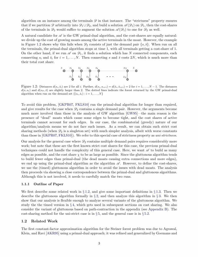
A natural candidate for A is the GW primal-dual algorithm, and the cost-shares are equally natural:we divide up the cost of growing moats among the active terminals in the moat. However, the examplein Figure 1.2 shows why this fails when D2 consists of just the demand pair s, s. When run on allthe terminals, the primal-dual algorithm stops at time 1, with all terminals getting a cost-share of 1.On the other hand, if we run A on D1, it finds a solution which has N connected components, eachconnecting si and si for i = 1, . . . , N . Then connecting s and s costs 2N , which is much more thantheir total cost share.

s1

s1

s2

s2

s3

s3

s4

s4

sN

sN

ss

Figure 1.2: Distances d(si, si) are 2 for all i. Further, d(si, si+1) = d(si, si+1) = 2 for i = 1, . . . , N − 1. The distancesd(s, s1) and d(sN , s) are slightly larger than 2. The dotted lines indicate the forest returned by the GW primal-dualalgorithm when run on the demand set (si, si) : i = 1, . . . , N

To avoid this problem, [GKPR07, FKLS10] run the primal-dual algorithm for longer than required,and give results for the case when D2 contains a single demand pair. However, the arguments becomemuch more involved than those in the analysis of GW algorithm [GW95]—the main reason is thepresence of “dead” moats which cause some edges to become tight, and the cost shares of activeterminals cannot account for such edges. In our case, the combinatorial (greedy) nature of ouralgorithm/analysis means we do not face such issues. As a result, we can obtain such strict costsharing methods (when D2 is a singleton set) with much simpler analysis, albeit with worse constantsthan those in [GKPR07, FKLS10]). We refer to this special case of strictness property as uni-strictness.

Our analysis for the general case where D2 contains multiple demand pairs requires considerably morework; but note that these are the first known strict cost shares for this case, the previous primal-dualtechniques could not handle the complexity of this general case. Here, we want A to build as manyedges as possible, and the cost share χ to be as large as possible. Since the gluttonous algorithm tendsto build fewer edges than primal-dual (the dead moats causing extra connections and more edges),we end up using the primal-dual algorithm as the algorithm A . However, to define the cost-shares,we use the (timed) gluttonous algorithm in order to avoid the issues with dead moats. The analysisthen proceeds via showing a close correspondence between the primal-dual and gluttonous algorithms.Although this is not involved, it needs to carefully match the two runs.

1.1.1 Outline of Paper

We first describe some related work in § 1.2, and give some important definitions in § 1.3. Then wedescribe the gluttonous algorithm formally in § 2, and then analyze this algorithm in § 3. We thenshow that our analysis is flexible enough to analyze several variants of the gluttonous algorithm. Westudy the the timed version in § 4, which gets used in subsequent sections on cost sharing. We alsoconsider the variant of gluttonous based on path-contraction in the appendix (see Appendix B). Thecost-sharing method for the uni-strict case is in § 5, and the general case is in § 5.2.

1.2 Related Work

The first constant-factor approximation algorithm for the Steiner forest problem was due to Agrawal,Klein, and Ravi [AKR95] using a primal-dual approach; it was refined and generalized by Goemans and

3

Williamson [GW95] to a wider class of network design problems. The primal-dual analysis also boundsintegrality gap of the the natural LP relaxation (based on covering cuts) by a factor of 2. Differentapproximation algorithms for Steiner forest based off the same LP, and achieving the same factor of2, are obtained using the iterative rounding technique of Jain [Jai01], or the integer decompositiontechniques of Chekuri and Shepherd [CS09]. A stronger LP relaxation was proposed by Konemann,Leonardi, and Schafer [KLS05], but it also has an integrality gap of 2 [KLSvZ08].

The special case of the Steiner tree problem, where all the demands share a common (source) terminal,has been well-studied in the network design community. There is a simple 2-approximation algorithmfor this problem: iteratively find the closest terminal to the source vertex, and merge these twoterminals. There have been several changes to this simple greedy algorithm leading to improvedapproximation ratios (see e.g. [RZ05]). Byrka et al. [BGRS13] improved these results to a ln 4 + ε ≈1.46-approximation algorithm, which is based on rounding a stronger LP relaxation for this problem.

The stochastic Steiner tree/forest problem was defined by Immorlica, Karger, Minkoff, and Mir-rokni [IKMM04], and further studied by [GPRS11], who proposed the boosted-sampling framework ofalgorithms. The analysis of these algorithms is via “strict” cost sharing methods, which were studiedby [GKPR07, FKLS10]. A constant-factor approximation algorithm (with a large constant) was givenfor stochastic Steiner forest by [GK09] based on primal-dual techniques; it is much more complicatedthan the algorithm and analysis based on the greedy techniques in this paper.

1.3 Preliminaries

Let M = (V, d) be a metric space on n points; assume all distances are either 0 or at least 1. Let thedemands D ⊆

(V2

)be a collection of source-sink pairs that need to be connected. By splitting vertices,

we may assume that the pairs in D are disjoint. A node is a terminal if it belongs to some pair in D .Let K denote the number of terminals pairs, and hence there are 2K terminals. For a terminal u, letu be the unique vertex such that u, u ∈ D ; we call u the mate of u.

For a Steiner forest instance I = (M,D), a solution F to the instance I is a forest such that eachpair u, u ∈ D is contained within the vertex set V (T ) for some tree T ∈ F . For a tree T = (V,ET ),let cost(T ) :=

∑e∈ET

d(e) be the sum of lengths of edges in T . Let cost(F ) :=∑

T∈F cost(T ) be thecost of the forest F . Our goal is to find a solution of minimum cost.

2 The Gluttonous Algorithm

To describe the gluttonous algorithm, we need some definitions. Given a Steiner forest instanceI = (M,D), a supernode is a subset of terminals. A clustering C = S1, S2, . . . , Sq is a partitionof the terminal set into supernodes. The trivial clustering places each terminal in its own singletonsupernode. Our algorithm maintains a clustering at all points in time. Given a clustering, a terminalu is active if it belongs to a supernode S that does not contain its mate u. A supernode S is active ifit contains some active terminal. In the trivial clustering, all the terminals and supernodes are active.

Given a clustering C = (S1, S2, . . . , Sq), define a new metric M/C called the C -puncturing of metricM. To get this, take a complete graph on V ; for an edge u, v, set its length to be d(u, v) if u, vlie in different supernodes in C , and to zero if u, v lie in the same supernode in C . Call this graphGC , and defined the C -punctured distance to be the shortest-path distance in this graph, denoted bydM/C (·, ·). One can think of this as modifying the metric M by collapsing the terminals in each ofthe supernodes in C to a single node. Given clustering C and two supernodes S1 and S2, the distancebetween them is naturally defined as

dM/C (S1, S2) = minu∈S1,v∈S2

dM/C (u, v).

4

The gluttonous algorithm is as follows:

Start with C being the trivial clustering, and E′ being the empty set. While there existactive supernodes in C , do the following:

(i) Find active supernodes S1, S2 in C with minimum C -punctured distance. (Break tiesarbitrarily but consistently, say choosing the lexicographically smallest pair.)

(ii) Update the clustering to

C ← (C \ S1, S2) ∪ S1 ∪ S2,

(iii) Add to E′ the edges corresponding to the inter-supernode edges on the shortest pathbetween S1, S2 in the graph GC .

Finally, output a maximal acyclic subgraph F of E′.

Above, we say we merge S1, S2 to get the new supernode S1∪S2. The merging distance for the mergeof S1, S2 is the C -punctured distance dM/C (S1, S2), where C is the clustering just before the merge.Since each active supernode contains an active terminal, if u ∈ S1 and v ∈ S2 are both active, thenwhen we talk about merging u, v, we mean merging S1, S2.

Note that the length of the edges added in step (iii) is equal to dM/C (S1, S2). The algorithm main-tains the following invariant: if S is a supernode, then the terminals in S lie in the same connectedcomponent of F .1 The algorithm terminates when there are no more active terminals, so each termi-nal shares a supernode with its mate, and hence the final forest F connects all demand pairs. Sincethe edges added to E′ have total length at most the sum of the merging distances, and we output amaximal sub-forest of E′, we get:

Fact 2.1 The cost of the Steiner forest solution output is at most the sum of all the merging distances.

We emphasize that the edges added in Step (iii) are often overkill: the metricM/E′ (where the edgesin E′ have been contracted) has no greater distances than the metric M/C that we focus on. Theadvantage of the latter over the former is that distances in M/C are well-controlled (and distancesbetween active terminals only increase over time), whereas those in M/E′ change drastically overtime (with distances between active terminals changing unpredictably).

s2s2 s1 s1s3

s3

3

22 11.5

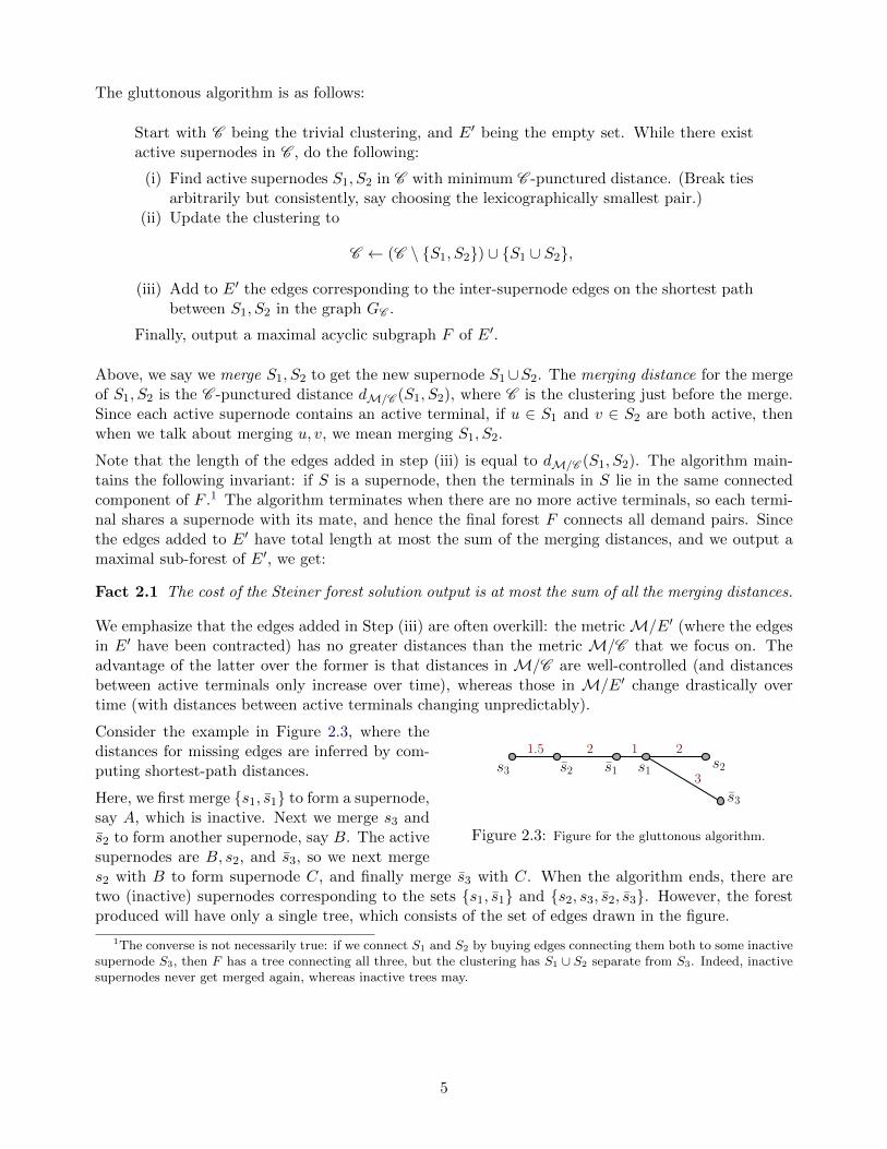
Figure 2.3: Figure for the gluttonous algorithm.

Consider the example in Figure 2.3, where thedistances for missing edges are inferred by com-puting shortest-path distances.

Here, we first merge s1, s1 to form a supernode,say A, which is inactive. Next we merge s3 ands2 to form another supernode, say B. The activesupernodes are B, s2, and s3, so we next merges2 with B to form supernode C, and finally merge s3 with C. When the algorithm ends, there aretwo (inactive) supernodes corresponding to the sets s1, s1 and s2, s3, s2, s3. However, the forestproduced will have only a single tree, which consists of the set of edges drawn in the figure.

1The converse is not necessarily true: if we connect S1 and S2 by buying edges connecting them both to some inactivesupernode S3, then F has a tree connecting all three, but the clustering has S1 ∪ S2 separate from S3. Indeed, inactivesupernodes never get merged again, whereas inactive trees may.

5

3 The Analysis for Gluttonous

We analyze the algorithm in two steps. One conceptual problem is in controlling what happens whengluttonous connects two nodes in different trees of the optimal forest. To handle this, we show in§ 3.2 how to preprocess the optimal forest F ? to get a near-optimal forest F ?? such that the finalclustering of the gluttonous algorithm is a refinement of this near-optimal forest. (I.e., if u and vare in the same supernode in the gluttonous clustering, then they lie in the same tree in F ??.) Thismakes it easier to then account for the total merging distance, which we do in § 3.3.

3.1 Monotonicity Properties

To begin, some simple claims about monotonicity. The first one is by definition.

Fact 3.1 (Distance Functions are Monotone) Let the clustering C ′ correspond to a later timethan the clustering C . Then C is a refinement of C ′. Moreover, dM/C ′(u, v) ≤ dM/C (u, v) for allu, v ∈ V .

Claim 3.2 Consider clustering C and let any two active supernodes S, T be merged, resulting inclustering C ′. Then for any active U ∈ C that is not S or T , the distance to its closest activesupernode does not decrease. Also, if S ∪ T is active in C ′ then the distance to its closest supernodein C ′ is at least as large as the minimum of S and T ’s distances to their closest supernodes in C .

Proof. First observe that when two active supernodes are merged, they may stay active or becomeinactive. An inactive supernode never merges with any other supernode, and hence, it cannot becomeactive later.

For active supernode U 6= S, T , suppose its closest supernode in C was W at C -punctured distanceL, and in C ′ it is W ′ at C ′-punctured distance L′. If L′ < L, there must now be a path throughsupernode S ∪ T that is of length L′. But this means the C -punctured distance of U from either S orT was at most L′, and both were active in C —a contradiction. This proves the first part of the claim.

Now, suppose supernode U := S ∪ T is active in C ′. Observe that for any other supernode W ∈ C ′,the punctured distance dM/C ′(U,W ) = mindM/C (S,W ), dM/C (T,W ). This proves the second partof the claim.

Claim 3.3 (Gluttonous Merging Distances are Monotone) If S, T are merged before S′, T ′ ingluttonous, then the merging distance for S, T is no greater than the merging distance for S′, T ′.

Proof. Gluttonous merges two active supernodes with the smallest current distance. By Claim 3.2distances between the remaining active supernodes do not decrease. This proves this claim.

3.2 A Near-Optimal Solution with Good Properties

Since gluttonous is deterministic and we break ties consistently, given an instance Steiner forestinstance I = (M,D) there is a unique final clustering C f produced by the algorithm.

Definition 3.4 (Faithful) A forest F is faithful to a clustering C if each supernode S ∈ C iscontained within a single tree in F . (I.e., for all S ∈ C , there exists T ∈ F such that S ⊆ V (T ).)

Note that every forest is faithful to the trivial clustering consisting of singletons.

Definition 3.5 (Width) For a forest F that is a solution to instance I , and for any tree T ∈ F ,let width(T ) denote the largest tree distance between any pair connected by T . Let the width of forestF be the sum of the widths of the trees in F . I.e.,

width(T ) := maxdT (u, u) | u, u ∈ D , u, u ⊆ V (T ), (3.1)

6

width(F ) :=∑

T∈F width(T ), (3.2)

where dT refers to the tree metric induced by T .

We now show there exist near-optimal solutions which are faithful to gluttonous’ final clustering.

Theorem 3.6 (Low-Cost and Faithful) Let F ? = T ?1 , T ?2 , . . . , T ?p be an optimal solution to theSteiner forest instance I = (M,D). There exists another solution F ?? for instance I such that

(a) cost(F ??) ≤ cost(F ?) + width(F ?) ≤ 2cost(F ?), and(b) F ?? is faithful to the final clustering C f produced by the gluttonous algorithm.

Proof. Start with F ?? = F ? which clearly satisfies the first (cost) guarantee but perhaps not thesecond (faithfulness) one. To fix this, run the gluttonous algorithm on I , and whenever it connectstwo terminals (u, v) that violate the condition (b), connect up some trees in the current F ?? to preventthis violation. In particular, we show how to do this while maintaining two invariants:

(A) The cost of edges in F ?? \F ? is at most width(F ?)− width(F ??), and

(B) at any point in time, the forest F ?? is faithful to the current clustering C (during the run ofthe gluttonous algorithm).

At the beginning, the clustering C is the trivial clustering consisting of singleton sets containingterminals, and F ?? = F ?; both invariants (A) and (B) are vacuously true.

Now consider some step of gluttonous which starts with the clustering C and connects two activesupernodes S and S′ which are closest to each other to get the clustering C ′. By the invariant (B),we know all terminals in supernode S lie within the same tree in F ??, and the same for terminals inS′. Let u ∈ S and v ∈ S′ be some active terminals within these supernodes; hence u 6∈ S and v 6∈ S′.Two cases arise:

• Case I: u and v belong to the same tree in F ??: Clearly, F ?? satisfies the invariant (B) withrespect to C ′ as well. Hence, we keep F ?? unchanged and it satisfies invariant (A) trivially.

• Case II: u and v belong to different trees T ??1 , T ??2 ∈ F ??: Suppose the shortest path betweenu and v in M/C is

P = u = x0, x′0, x1, x

′1, x2, x

′2, x3, . . . , x

′k−1, xk, x

′k = v

such that each xi, x′i belong to the same supernode Si in C (see e.g., figure 3.4). By the greedy

behavior of gluttonous, cost(P ) is at most the cost to connect u to u, or to connect v to v inM/C . In fact, we can bound these costs by the cost of the edges between u, u in T ??1 , etc.Hence,

cost(P ) ≤ mindT ??

1(u, u), dT ??

2(v, v)

≤ min

width(T ??1 ),width(T ??2 )

. (3.3)

Since each of the supernodes Si is contained within some tree in F ?? (by invariant (B) appliedto clustering C ), we need only add (a subset of edges from) the path P to the forest F ?? inorder to merge T ??1 and T ??2 (and perhaps other trees in F ??) into one single tree—thus ensuringinvariant (B) for the new clustering C ′.

How does the width of the trees in F ?? change? Each tree that we merge is inactive (since itis a coarsening of the original solution F ?). Connecting up T ??1 , . . . , T ??k causes the width ofthe resulting tree to be maxwidth(T ??1 ), · · · ,width(T ??k ). The decrease in width(F ??) due tothe merge is at least minwidth(T ??1 ),width(T ??2 ), which ensures invariant (A) (using inequal-ity (3.3)).

7

ux′0 x1

x′1

x2

x′2 x3

v

Figure 3.4: Case II of the proof of Theorem 3.6. The grey blobs are supernodes in C , the solid lines denote the forestF ??. The dotted lines are the path P . Observe we do not need to add the second edge of P as it will create a cycle.

Hence, at the end of the run of gluttonous, both invariants hold. Since the initial potential iswidth(F ?) ≤ cost(F ?), and the final potential is non-negative, the total cost of edges in F ?? \F ? isat most cost(F ?). This completes the proof.

3.3 Charging to this Near-optimal Solution

Let F ? = T ?1 , . . . , T ?p be a solution to the Steiner forest instance. The main result of this section is:

Theorem 3.7 If the forest F ? is faithful to the final clustering C f of the gluttonous algorithm, thenthe cost of the gluttonous algorithm is O(1) · cost(F ?).

Since by Theorem 3.6 there is a forest F ? with cost at most twice the optimum that is faithful togluttonous’ final clustering C f , applying Theorem 3.7 to this forest proves Theorem 1.1.

We now prove Theorem 3.7. At a high level, the proof proceeds thus: we consider the run of thegluttonous algorithm, and maintain for each iteration t a “candidate” forest Ft that is a solutionto the remaining instance. We show that in an amortized sense, at each step the cost of forest Ft

decreases by an amount which is a constant fraction of the cost incurred by gluttonous. Since thestarting cost of this forest is at most a constant times the optimal cost, so is the total merging costof the gluttonous, proving the result.

For Steiner forest instance I , assume that C f is gluttonous’ final clustering, and F ? is faithful to C f .Let C (t) be the gluttonous clustering at the beginning of the iteration t, with C

(t)active being the active

supernodes. It will be useful to view this clustering as giving us an induced Steiner forest instance It

on the metric whose points are the supernodes in C (t) and where distances are given by the puncturedmetric dM/C (t) , where the terminals in the instance It are supernodes in C

(t)active, and where active

supernodes S1, S2 are mates if there is a pair u, u such that u ∈ S1 and u ∈ S2. (Supernodes nolonger have unique mates, but this property was only used for convenience in Theorem 3.6). For anyiteration t, the subsequent run of gluttonous is just a function of this induced instance It. Indeed,given the instance It, gluttonous outputs a final clustering which is same as C f except the inactivesupernodes in C (t) are absent. I.e., the inactive supernodes in C (t) will not play a role, but all theactive supernodes will continue to combine in the same way in It as in I . We now inductivelymaintain a forest F (t) such that

(I1) F (t) is a feasible solution to this Steiner forest instance It, and(I2) F (t) maintains the connectivity structure of F ?, i.e., if u and v are two active terminals which

are in the same tree in F ?, then the supernodes containing u and v lie in the same tree in F (t).

And we will charge the cost of gluttonous to reductions in the cost of this forest F (t).

The “candidate” forest F (t). The initial clustering C (1) is the trivial clustering consisting ofsingleton terminals; we set F (1) to F ?. Since I1 is the original instance, F (1) is feasible for it;invariant (I2) is satisfied trivially.

8

For an iteration t, let E(F (t)) denote the edges in F (t). Note that an edge e ∈ E(F (t)) between twosupernodes S1, S2 ∈ C (t) corresponds to an edge between two terminals u, v in the original metricM,where u ∈ S1, v ∈ S2. Define length(e) as dM(u, v), the length of the edge e in the original metric.Note that the length of e in the metricM/C (t) may be smaller than length(e). For every edge e ∈ F (t),we shall also maintain a potential of e, denoted ψ(e). Initially, for t = 1, the potential ψ(e) = length(e)for all e ∈ E(F (1)). During the course of the algorithm, the potential ψ(e) ≥ length(e); we describethe rule for maintaining potentials below. Intuitively, an edge e ∈ F (t) would have been obtained byshort-cutting several edges of F ?, and ψ(e) is equal to the total length of these edges.

Suppose we have a clustering C (t−1) and a forest F (t−1) which satisfies invariants (I1) and (I2). If wenow merge two supernodes S1, S2 ∈ C (t−1) to get clustering C (t), we have to update the forest F (t−1)

to get to F (t) using procedure UpdateForest given in Figure 3.3. The main idea is simple: whenwe merge the nodes corresponding to S1 and S2 in F (t−1) into a single node, this creates a cycle.Removing any edge from the cycle maintains the invariants, and reduces the cost of the new forest:we remove the edge with the highest potential from the cycle. We further reduce the cost by gettingrid of Steiner vertices, which correspond to inactive supernodes in F (t) with degree 2. More formally,given two edges e′ = u′, v, e′′ = u′′, v with a common end-point v, the operation short-cut on e′, e′′

replaces them by a single edge u′, u′′. Whenever we see a Steiner vertex of degree 2 in F (t), weshortcut the two incident edges.

Algorithm UpdateForest (C (t−1), S1, S2) :

1. Let T be the tree in F (t−1) containing the terminals in S1 and S2.2. Merge S1 and S2 to a single node S in the tree T .3. If the new supernode S becomes inactive, and has degree 2 in the tree T , then

short-cut the two edges incident to S.4. Let C denote the unique cycle formed in the tree T .5. Delete the edge in the cycle C which has the highest potential.6. While there is an inactive supernode in T which is a degree-2 vertex,

short-cut the two incident edges to this vertex.

Figure 3.5: The procedure for updating F (t−1) to F (t).

Some more comments about the procedure UpdateForest. In Step 1, the existence of the tree Tfollows from the invariant property (I2) and the faithfulness of F ? to C f . Since the terminals inS1 ∪ S2 are in the same tree in F ?, the invariant means they belong to the same tree in F (t−1), andthe construction ensures they remain in the same tree in F (t). When we short-cut edges e′, e′′ toget a new edge e, we define the potential of the new edge e to be ψ(e) := ψ(e′) + ψ(e′′). It is alsoeasy to check that F (t) is a feasible solution to the instance It. Indeed, the only difference betweenIt−1 and It is the replacement of S1, S2 by S. If S becomes inactive, there is nothing to prove. If Sremains active, then the tree containing S must will also have also have the supernodes which werepaired with S1 and S2 in the instance It−1. It is also easy to check that the invariant property (I2)continues to hold. The following claim proves some more crucial properties of the forest F (t).

Claim 3.8 For all iterations t, the Steiner nodes in F (t) have degree at least 3. Therefore, there areat most 2 iterations of the while loop in Step 6 of the UpdateForest algorithm.

Proof. We prove the first statement of the lemma by induction on t. For t = 1, it holds by construc-tion: we can assume that F ? has no Steiner vertex of degree at most 2: any leaf Steiner node can bedeleted, and a degree 2 can be removed by short-cutting the incident edges. Suppose this property istrue for F (t−1). We merge S′ and S′′, and if the new supernode S becomes an inactive supernode,

9

then its degree will be at least 2 (both S′ and S′′ must have had degree at least 1). If the degree isequal to 2, we remove this vertex in Step 3.

When we remove an edge in Step 5, the two end-points could have been Steiner vertices. By theinduction hypothesis, their degree will be at least 2 (after the edge removal). If their degree is 2, wewill again remove them by short-cutting edges. Note that this will not affect the degree of other nodesin the forest. This also shows that Step 6 will be carried out at most twice.

Here’s the plan for rest of the analysis. Let’s fix a tree T ? of F ?, and account for only those mergingcosts which merge two supernodes with terminals in T ?. (Summing over all trees in F ? and using thefaithfulness of F ? to C f will ensure all merging costs are accounted for.) Since F (t) is obtained byrepeatedly contracting nodes and removing unnecessary edges, in each iteration t there is a unique treeT (t) in the forest F (t) corresponding to the tree T ?, namely the tree containing the active supernodeswith terminals belonging to T ?. Call an iteration of the gluttonous algorithm a relevant iteration(with respect to T ?) if gluttonous merges two supernodes from the tree T (t) in this iteration. Forbrevity, we drop the phrase “w.r.t. T ?” in the sequel.

Next we show that the total potential of the edges does not change over time. Let del(t) denote the setof edges which are deleted (from a cycle in Step 5) during the (relevant) iterations among 1, . . . , t− 1.(Observe that del(t) does not include edges that are short-cut.)

Lemma 3.9 For iteration t, the sum of potentials of edges del(t) and E(T (t)) equals cost(T ?). Further,ψ(e) ≥ length(e) for all edges e ∈ E(T (t)) ∪ del(t).

Proof. By induction on t. The base case t = 1 follows by construction. For the IH, assume thestatement holds for t− 1. Assume that t is a relevant iteration (else T (t) = T (t−1)): if we remove edgee from T (t−1) during Step 5, we do not change ψ(e). If we short-cut two edges e′, e′′ to an edge e,ψ(e) = ψ(e′) + ψ(e′′). Therefore the total potential of the edges in the tree plus that of the edges indel(t) does not change. Further, length(e) ≤ length(e′) + length(e′′) ≤ ψ(e′) + ψ(e′′) = ψ(e).

Eventually T (t) has no active supernodes (for large t) and hence all its edges are deleted. Hence ifdel(∞) denotes the edges deleted during all the relevant iterations in gluttonous, Lemma 3.9 implies∑

e∈del(∞) ψ(e) = cost(T ?). Let ∆t denote the merging cost of some relevant iteration t: we now showhow to charge this cost to the potential of some deleted edge in del(∞). Formally, let Nt denote thenumber of active supernodes in T (t), at the beginning of iteration t.

Theorem 3.10 If t0 is relevant, there are at least Nt0/8 edges in del(∞) of potential at least ∆t0/6.

We defer the proof of Theorem 3.10 for the moment, and instead show how to use this to charge themerging costs and to prove Theorem 3.7, which in turn gives the main theorem of the paper.

Proof of Theorem 3.7: Let Ir denote the index set of all relevant iterations during the run ofgluttonous. We now define a mapping g from Ir to del(∞) such that: (i) for any edge e ∈ del(∞),the pre-image g−1(e) has cardinality at most 8, and (ii) the potential ψ(g(t)) ≥ ∆t/6 for all t ∈ Ir.To get this, consider a bipartite graph on vertices Ir ∪ del(∞) where a iteration t ∈ Ir is connectedto all edges e ∈ del(∞) for which ψ(e) ≥ ∆t/6. Theorem 3.10 shows this graph satisfies a Hall-typecondition for such a mapping to exist; in fact a greedy strategy can be used to construct the mapping(there can be at most Nt relevant iterations after iteration t because each relevant iteration reducesthe number of active supernodes by at least one).

Thus, the total merging cost of gluttonous during relevant iterations is at most∑t∈Ir

∆t =∑

e∈del(∞)

∑t∈g−1(e)

∆t ≤ 48∑

e∈del(∞)

ψ(e) = 48 cost(T ?),

10

where the last equality follows from Lemma 3.9. By the faithfulness property, each iteration ofgluttonous is relevant with respect to one of the trees in F ?, so summing the above expression overall trees gives the total merging cost to be at most 48 cost(F ?).

Combining Theorem 3.7 with Theorem 3.6 gives an approximation factor of 96 for the gluttonousalgorithm. While we have not optimized the constants, but it is unlikely that our ideas will lead toconstants in the single digits. Obtaining, for instance, a proof that the gluttonous algorithm is a2-approximation (or some such small constant) remains a fascinating open problem.

3.3.1 Proof of Theorem 3.10

In order to prove Theorem 3.10, we need to understand the structure of the trees T (t) for t ≥ t0 inmore detail. Let del0([t0 . . . t)) denote the edges deleted during the relevant iterations in t0, . . . , t− 1,i.e., del([t0 . . . t)) := del(t) \ del(t0). Observe that each edge of T (t) is either in T (t0) or is obtained byshort-cutting some set of edges of T (t0). Hence we maintain a partition E (t) of the edge set E(T (t0)),such that there is a correspondence between edges e ∈ T (t) ∪ del([t0 . . . t)) and sets Dt(e) ∈ E (t), suchthat Dt(e) is the set of edges in T (t0) which have been short-cut to form e.

For each set Dt(e), let head(Dt(e)) be the edge e′ ∈ Dt(e) with greatest length. If edge e is removedfrom T (t) in some relevant iteration t, we have e ∈ del([t0 . . . t

′)) for all t′ > t, and the set Dt′(e) = Dt(e)for all future partitions E (t′).

Lemma 3.11 There are at least Nt0/2 edges of length at least ∆t0/6 in tree T (t0).

Proof. Call an edge long if its length is at least ∆t0/6, and let ` denote the number of long edges inthe tree T (t0). Deleting these edges from T (t0) gives ` + 1 subtrees C1, C2, . . . , Cl+1. Let Ci have niactive supernodes and ei edges. For each tree Ci where ni ≥ 2, take an Eulerian tour Xi and divideit into ni disjoint segments by breaking the tour at the active supernodes. Each edge appears in twosuch segments, and each segment has at least six edges (since the distance between active supernodesis at least ∆t0 and none of the edges are long), so ei ≥ 3ni when ni ≥ 2. This means the total numberof edges in T (t0) is at least three times the number of “social” supernodes (supernodes that do not liein a component Ci with ni = 1, in which they are the only supernode), plus those ` long edges thatwere deleted.

And how many such social supernodes are there? If ` ≥ Nt0 + 1, there may be none, but then weclearly have at least Nt0/2 long edges. Else at least Nt0 − ` supernodes are social, so T (t0) has at least3(Nt0 − `) + ` edges. Finally, since every Steiner vertex in T (t0) has degree at least 3, the number ofedges is less than 2Nt0 . Putting these together gives 3Nt0 − 2` ≤ 2Nt0 or ` ≥ Nt0/2.

Let L0 be the set of long edges in T (t0), and E (∞) be the partition at the end of the process. Twocases arise:

• At least Nt0/8 edges in L0 are head(D∞(e)) for some set D∞(e) ∈ E (∞). Since each setin E (∞) has only one head, there are Nt0/8 such sets. In any such set D∞(e), ψ(e) ≥length(head(D∞(e))) ≥ ∆t0/6. Moreover, we must have removed e in some iteration between t0and the end, and hence e ∈ del([t0 . . .∞)) ⊆ del(∞).

• More than than 3Nt/8 edges in L0 are not heads of any set in E (∞). Take one such edge e0 —the sets in E (t0) are singleton sets and hence e0 is the head of the set Dt0(e0). Let t be the first(relevant) iteration such that e0 is not the head of the set containing it in E (t), and supposee0 = head(Dt−1(e′)) for some set Dt−1(e′) ∈ E (t−1). In forming F (t), we must have short-cut e′

and some other edge e′′ to form an edge e ∈ F (t). Observe that length(head(D(e′′)) ≥ length(e0),

11

else e0 would continue to be the head of D(e). Moreover,

min(ψ(e′), ψ(e′′)

)≥ min

(length(head(e′)), length(head(e′′))

)≥ ∆t0/6.

By the discussion in Claim 3.8, one of e′ and e′′ must lie on the cycle formed when we mergedtwo supernodes in F (t−1), as in Step 4 of UpdateForest. Further, if et was the edge removedfrom this cycle, by the rule in Step 5 we get that the potential ψ(et) is the maximum potentialof any edge on this cycle, and hence ψ(et) ≥ min(ψ(e′), ψ(e′′)) ≥ ∆t0/6. Hence we want to“charge” this edge e0 ∈ L0 to et ∈ del(∞) (which has potential at least ∆t0/6). However, upto three edges from L0 may charge to et: this is because there can be at most three short-cutoperations in any iteration (one from Step 3 and two from Step 6).

In both cases, we’ve shown the presence of at least Nt0/8 edges in del(∞) of potential ∆t0/6, whichcompletes the proof of Theorem 3.10.

3.4 An Extension of the Analysis in Section 3

Let us now abstract out some properties used in the above analysis, so that we can generalize theanalysis to a broader class of algorithms for Steiner forest. This abstraction is used to show thatvariants of the above algorithm, which are presented in Section 4 and in Appendix B, are also O(1)-approximations.

Consider an algorithm A which maintains a set of supernodes, where a supernode corresponds to aset of terminals, and two different supernodes correspond to disjoint terminals. Initially, we have onesupernode for each terminal. Further, a supernode could be active or inactive. Once a supernodebecomes inactive, it stays inactive. Now, at each iteration, the algorithm picks two active supernodes,and replaces them by a new supernode which is the union of the terminals in these two supernodes(the new supernode could be active or inactive). Note that the iteration when a supernode becomesinactive is arbitrary (depending on the algorithm A ).

As in the case of gluttonous algorithm, let C f be the final clustering produced by the algorithm A ,and T ? be a tree solution to a Steiner forest instance (D ,M). Let C (t) be the set of supernodes atthe beginning of iteration t of A . For an iteration t, let δt be the minimum distance (in the metricM/C (t)) between any two active supernodes in C (t). Claim 3.2 gives the following fact.

Fact 3.12 The quantity δt forms an ascending sequence with respect to t.

Now Theorem 3.7 generalizes to the following stronger result.

Corollary 3.13 For any tree solution T ? to an instance I ,∑

t δt ≤ 48 · cost(T ?).

An important remark: this corollary is not making any claim about the merging cost of A ; at anyiteration A could be connecting two active supernodes which are much farther apart than δt.

4 A Timed Greedy Algorithm

We now give a version of the gluttonous algorithm TimedGlut where supernodes are deemed activeor inactive based on the current time and not whether the terminals in the supernode have paired upwith their mates.2 This version will be useful in getting a strict cost-sharing scheme.

2Timed versions of the primal-dual algorithm for Steiner forest had been considered previously in [GKPR07, KLS05];our version will be analogous to that of Konemann et al. [KLS05] which were used to get cross-monotonic cost-sharesfor Steiner forest.

12

The algorithm TimedGlut is very similar to the gluttonous algorithm except for what constitutes anactive supernode.

We will again maintain a clustering of terminals (into supernodes) – let C (t) be the clustering atthe beginning of iteration t. Initially, at iteration t = 1, C (1) is the trivial clustering (consisting ofsingleton sets of terminals). We maintain a set of edges E′ will be the set of edges bought by thealgorithm. Initially, E′ = ∅.We shall use ∆t to denote the closest distance (in the metricM/C (t)) between two active supernodesin C (t). Our algorithm will only merge active supernodes, and an inactive supernode will not becomeactive in future iterations. It follows that ∆t cannot decrease with t (Fact 3.1). This allows us todivide the execution of the algorithm into stages. Stage i consists of those iterations t for which ∆t

lies in the range [2i, 2i+1) (the initial stage belongs to stage 0, because we can assume w.l.o.g. thatthe minimum distance between the terminals is 1).

For a terminal s, define

level(s) := dlog2 dM(s, s)e. (4.4)

Note that distances in this definition are measured in the original metric M. For a supernode S,define its leader as the terminal in S whose distance to its mate is the largest (and hence has thelargest level); in case of ties, choose the terminal with the smallest index among these.

We shall use C i to denote the clustering at the beginning of stage i (note the change in notation withrespect to the clustering at the beginning of an iteration t, which will be denoted by C (t). So, if tidenotes the first iteration of stage i, then C i is same as C (ti)). Now we specify when a supernodebecomes inactive. A terminal s is active at the beginning of stage i if level(s) ≥ i. A supernode S willbe active at the beginning of a stage i if level(leader(S)) ≥ i. Observe that supernodes do not becomeinactive during a stage – if a terminal is active at the beginning of a stage, it remains active duringeach of the iterations in this stage.

By the definition of a stage, the algorithm will satisfy the invariant that the distance between any twoactive supernodes in C i (in the metricM/C i) is at least 2i. During stage i, the algorithm repeatedlyperforms the following steps in each iteration t: pick any two arbitrary pair of active supernodes S′, S′′

which are at most 2i+1 apart (in the metricM/C (t)). Further, we take any such S′-S′′ path of lengthat most 2i+1 (in the graph induced by the metric M/C (t) on the vertex set C (t)) and add the edges(which go between supernodes) to E′.

Stage i ends when the merging distance between all remaining active supernodes is at least 2i+1.Observe that when the algorithm stops, we have a feasible solution—indeed, each terminal s willmerge with its mate s by the end of stage level(s). At the end, output a maximal acyclic subgraph ofE′.

The analysis of TimedGlut goes along the same lines as that of the gluttonous algorithm. The analogof Theorem 3.6 is as follows:

Theorem 4.1 Let F ? = T ?1 , T ?2 , . . . , T ?p be an optimal solution to the Steiner forest instance I =

(M,D). Let clustering C f be produced by some run of the TimedGlut algorithm. There exists anothersolution F ?? for instance I such that

(a) cost(F ??) ≤ cost(F ?) + 4 · width(F ?) ≤ 5 · cost(F ?), and(b) F ?? is faithful to the clustering C f .

Proof. The proof is very similar to that of Theorem 3.6, where we look over the run of TimedGlutagain to alter F ? into F ??. Since TimedGlut makes some arbitrary choices, we make the same choicesconsistently in this proof. We ensure very similar invariants:

13

(A) The cost of edges in F ?? \F ? is at most 4(width(F ?)− width(F ??)), and

(B) at any point in time, the forest F ?? is faithful to the current clustering C .

Observe the extra factor of 4 in invariant (A). Again, let two active supernodes S′ and S′′ be mergedin some stage i, and let u and v be the leaders of these supernodes respectively. The argument inCase I remains unchanged. In Case II, let T ??1 and T ??2 be the trees containing u and v respectively.Being in stage i, we know that level(u), level(v) ≥ i, since they are both still active, and that thedistance between S′ and S′′ in the current metric is at most 2i+1, since all merging costs in stage i liebetween 2i and 2i+1. So the cost of connecting T ??1 and T ??2 is at most

2i+1 ≤ min(2level(u)+1, 2level(v)+1) ≤ 4 ·min(dT ??1

(u, u), dT ??2

(v, v))

≤ 4 ·min(width(T ??1 ),width(T ??2 )).

The rest of the argument remains unchanged.

Theorem 4.2 The TimedGlut algorithm is a γTG-approximation algorithm for Steiner forest, whereγTG = 96× 5 = 480.

Proof. Consider a solution F ?? which is faithful with respect to the final clustering produced by theTimedGlut algorithm. Suppose there are mi iterations during stage i. Then the total merging cost ofthe algorithm is at most

∑i 2i+1 ·mi.

We would like to use Corollary 3.13. Let F ?? consist of the trees T ??1 , . . . ,T ??

k . For a tree T ??r , and

a stage i, let Ii,r denote the iterations when we merge two supernodes with terminals belonging tothe tree V (T ??

r ) (note that the faithfulness property implies that there will be such a tree for eachiteration of the algorithm). Let mi,r denote the cardinality of Ii,r. Clearly,

∑rmi,r = mr. For an

iteration t, and index r, let C(t)r denote the supernodes in C (t) with terminals belonging to V (T ?r ).

Define δt,r as the closest distance (in the metric M/C (t)) between any two active supernodes withterminals belonging to V (T ?r ). If the iteration belongs to stage i, then δt,r ≥ 2i. Using Corollary 3.13,we get ∑

i

2i+1mi ≤ 2 ·∑r

∑i

2i ·mi,r ≤ 98 ·∑r

cost(T ?r ).

The result now follows from Theorem 4.1.

4.1 An Equivalent Description of TimedGlut

An essentially equivalent way to state the TimedGlut algorithm is as follows. For a stage i, let Mi

denote the metric M/C i corresponding to the clustering at the beginning of stage i. Construct anauxiliary graph H(i) with vertex set being the set of supernodes in C i, and edges between two verticesif the two corresponding supernodes are active and the distance between them is at most 2i+1 in themetric Mi. Pick a maximal acyclic set of edges P(i) in this auxiliary graph H(i).

• For each edge (S1, S2) ∈ P(i), merge the supernodes S1, S2. Hence the clustering C i+1 at theend of stage i is obtained by merging together all the supernodes that fall within a connectedcomponent of the subgraph (H(i),P(i)).• For each edge (S1, S2) ∈ P(i), add edges corresponding to a path of length < 2i+1 in Mi to a

set of edges Ei.

Finally, output a maximal sub-forest of the edges ∪iEi added during this process.

One can now check that this algorithm is equivalent to the TimedGlut algorithm as described above;the key observation is that because of the definition of the timed algorithm, an active terminal instage i stays active throughout the stage, and does not become inactive partway through it. Moreformally, we have the following observation.

14

Fact 4.3 Consider an execution of the TimedGlut algorithm on an input I . Then one can definegraphs H(i) and P(i) for each stage i such that the set of supernodes at the beginning of stage i inthe above algorithm is same as that of the TimedGlut algorithm. Further, the two algorithms pick thesame set of edges in each stage.

5 Cost Shares for Steiner Forest

A cost-sharing method is a function χ mapping triples of the form (M,D , (s, s)) to the non-negativereals, where (M,D) is an instance of the Steiner forest problem, and (s, s) ∈ D . We require thecost-sharing method to be budget-balanced : if F ? is an optimal solution to the instance (M,D) then∑

(s,s)∈D

χ(M,D , (s, s)) ≤ cost(F ?). (5.5)

We will consider strict cost-shares; these are useful for several problems in network design (see detailsin the introduction). There are two versions of strictness: uni-strictness, and strictness. Uni-strictcost-shares for Steiner forest were given by [GKPR07, FKLS10], whereas strict cost shares for Steinerforest have remained an open problem. We show how to get both using the TimedGlut algorithm.

5.1 Uni-strict Cost Shares for Steiner Forest

Definition 5.1 Given an α-approximation algorithm A for the Steiner forest problem, a cost sharingχ is called β-uni-strict with respect to A if for all demand pair (s, s), the cost share χ(M,D , (s, s))is at least 1/β times the distance between s and s in the graph G/F , where F is the forest returnedby algorithm A on the input (M,D − s, s).

Our objective is to find an algorithm A and the associated cost share χ such that the parameters αand β are both constants.

5.1.1 Defining χ and A

Let the constant γTG denote the approximation ratio of the algorithm TimedGlut. The cost-sharingmethod is simple: for a terminal s, let `s be the largest value such that s is a leader in stage `s andits supernode is merged with some other supernode during this stage (note that a supernode can gofrom being active in the beginning of a stage to becoming inactive in the next stage without mergingwith any supernode; this can happen because all terminals in it become inactive in the next stage).Then

χ(M,D , (s, s)) :=2`s + 2`s

2γTG

. (5.6)

The algorithm A is a slight variant on the TimedGlut algorithm. Given an instance (M,D), run thealgorithm TimedGlut on this instance to get forest F . Now merge some of the trees in F as follows.Recall that the width of each tree T in F is defined to be width(T ) := max(s,s)∈T dT (s, s), wheredT (s, s) denotes the distance between s and s in the tree T . While there are trees T1, T2 ∈ F suchthat dM/F (T1, T2) ≤ 5 min(width(T1),width(T2)), connect T1, T2 by a path of length dM/F (T1, T2) toget a tree T , and update F ← (F \ T1, T2) ∪ T. Here, dM/F (T1, T2) denotes the minimum overall pairs u ∈ T1, v ∈ T2, of dM/F (u, v).

15

5.1.2 Analysis

We now prove that the cost sharing method χ is β-uni-strict with respect to A , where β is a constant.Recall that F denotes the forest returned by the algorithm A .

To begin, observe that the algorithm A is also a constant-factor approximation.

Lemma 5.2 The algorithm A is an 6γTG-approximation for Steiner forest.

Proof. Let F ′ be the forest returned by the TimedGlut algorithm (called by A ). Consider thepotential

∑T∈F ′(c(T ) + 5width(T )). Since the width of each tree is at most the cost of its edges,

and since TimedGlut was a γTG-approximation, this potential is at most 6γTG times the optimal cost.Now, observe that whenever A merges two trees of this forest, the potential of the new forest doesnot increase. Therefore, the potential of the forest F is also at most 6γTG times the optimal cost.

Lemma 5.3 The function χ is a budget-balanced cost sharing method.

Proof. We need to prove the inequality (5.5). To do this, let us run TimedGlut and “charge” the costof merging two active supernodes to the leaders of the respective clusters—charge half of the distancebetween these two supernodes to the leaders of each of these supernodes. Clearly, the total chargeassigned to the terminals is equal to the total cost paid by the algorithm TimedGlut, which at mostγTG cost(F ?). Finally, we make the observation that each terminal s is charged at least γTG times thecost share (since it is charged at least 2`s/2 in stage `s) to complete the proof.

To prove the uni-strictness property, fix a terminal pair (s, s), and consider two instances: I = (M,D)and I ′ = (M,D − (s, s)). For instance I , let C i denote the set of supernodes at the beginningof stage i; let C

′i be the corresponding set for I ′. Let Mi and M′i denote the metrics M/C i andM/C

′i respectively. Recall that level(s) = dlog2 dM(s, s)e.The following claim will be convenient to understand the behavior of TimedGlut.

Lemma 5.4 Consider stage i in the execution TimedGlut on the instance I . Define a graph Gi onthe vertex set C i, with an edge between two active supernodes C1, C2 ∈ C i if there is a path of lengthat most 2i+1 between them in Mi that does not contain any other active supernode as an internalnode. If the connected components of Gi are H1, . . . ,Hq, then C i+1 has q supernodes—one supernodefor each Hj (formed by merging the supernodes in Hj).

Proof. The statement is essentially the same as Fact 4.3 except that in the graph H(i) (defined inSection 4.1), we join two active supernodes C1, C2 ∈ C i by an edge if the distance between them inthe metricMi is at most 2i+1, whereas here in the graph Gi, we wish to have a path of length at most2i+1 with no internal vertex being an active supernode. We claim that the connected components inthe two graphs are the same, and hence, the statement in the lemma follows.

Clearly, an edge e ∈ Gi is present in H(i) as well. Now, consider an edge (C1, C2) in H(i). Let Pbe the shortest path of length at most 2i+1 between S1 and S2 in the metric Mi. Let the activesupernodes on this path be C1 = Ci1 , Ci2 , . . . , Cip = C2 (in this order). Then Gi has edges (Cir , Cir+1)for r = 1, . . . , p − 1. Therefore C1 and C2 are in the same connected component of Gi. This provesthe desired claim.

Theorem 5.5 (Nesting) For i ≤ level(s), let Cs and Cs be the supernodes in C i containing s and srespectively. The following hold:

(a) If Cs 6= Cs, we can arrange the supernodes in C′i as C ′1, . . . , C

′p such that Cs = s∪C ′1∪. . .∪C ′a,

Cs = s∪C ′a+1∪ . . .∪C ′b for some 0 ≤ a ≤ b ≤ p. Moreover, C i−Cs, Cs = C ′b+1, . . . , C′p. If

Cs = Cs, we can arrange the supernodes in C′i as C ′1, . . . , C

′p such that Cs = s, s∪C ′1∪. . .∪C ′b,

for some 0 ≤ b ≤ p. Also, C i − Cs = C ′b+1, . . . , C′p.

16

(b) Suppose Cs and Cs are distinct supernodes. Then for any terminal v ∈ Cs, dM′i(s, v) ≤ 2 · 2i.Similarly, for any v ∈ Cs, dM′i(s, v) ≤ 2 · 2i.

(c) Suppose Cs = Cs. Then, dM′i(s, s) ≤ 4 · 2i.

Proof. We induct on i. At the beginning, all clusters are singletons, so the base case is easy. Forthe inductive step, suppose the statement of the theorem is true for some i < level(s). Assume thatCs 6= Cs, the other case is similar. Apply Lemma 5.4 to stage i in both I and I ′, and let Gi and G ′ibe the corresponding graphs on the vertex sets C i and C

′i (as defined in Lemma 5.4). We know thatthe supernodes of C i+1 and C

′i+1 correspond to the connected components of these graphs; we nowuse this information to prove the induction step.

By the induction hypothesis, the supernodes in C i can be labeled Cs, Cs, C′b+1, . . . , C

′p; moreover, we

can define a map φ : V (G ′i )→ V (Gi) as follows:

φ(C ′j) :=

Cs 0 ≤ j ≤ aCs a+ 1 ≤ j ≤ bC ′j b+ 1 ≤ j ≤ p

(5.7)

Suppose there is an edge between C ′j and C ′k in G ′i . By the definition of Gi, both are active supernodes,

and the length of the shortest path between them in the metric M′i is at most 2i+1. This path hasno greater length in the metricMi, since the supernodes in C i are unions of supernodes in C

′i. Thismeans there is a path between φ(C ′j) and φ(C ′k) in Gi, i.e., the clustering C

′i+1 is a refinement of C i+1

(because these clusterings are determined by the connected components of the corresponding graphs).

Now consider an edge e in Gi. For the first part of the theorem, suppose e = (C ′j , C′k) where both

j, k ≥ b + 1. If P is the corresponding path in Mi between these two supernodes, then P cannotcontain Cs or Cs as an internal node (because it does not contain any active supernodes as internalnodes, and both Cs, Cs are active). But then the length of P remains unchanged inM′i, and we havethe corresponding edge (C ′j , C

′k) in G ′i as well. This means that all the connected components of Gi

not containing Cs or Cs also form connected components in G ′i . Combined with the fact that C′i+1

is a refinement of C i+1, this proves the part (a) of the theorem for the case Cs 6= Cs. (The proof forthe other case is similar.)

For part (b), let H1 be the connected component of Gi which contains the supernode Cs (as a vertex).So all the supernodes in H1 will merge to form a single supernode of C i+1. As argued in the paragraphabove, any edge in H1 which is not incident with Cs is also present in G ′i (recall that we are assumingCs is not one of the vertices in H1). Let v be a terminal in a supernode B in H1. Let the path from Csto B in H1 be Cs = A0, A1, . . . , Ar = B. Since the edges (A1, A2), . . . , (Ar−1, Ar) belong to G ′i as well,A1, . . . , Ar will lie in the same supernode in C

′i+1. Therefore, dM′i+1(s, v) ≤ 2i+1 + 2 · 2i = 2 · 2i+1,

where the term 2 · 2i is present to account for the distance between s and the terminal in Cs which isclosest to A1 – this distance can be at most 2 · 2i by the induction hypothesis.

For part (c), consider the last stage i such that the supernodes Cs and Cs are distinct (so the resultin part (b) applies to this stage). The same argument as above applies except that when we considerthe path from Cs to Cs in the component of Gi containing them, we will have to account for the firstand the last edges in this path.

We are now ready to prove the uni-strictness of the cost-shares. We run TimedGlut on the instanceI to get the cost shares, and let the cost share for (s, s) be as in (5.6). Now let F ′ be the forestreturned by the algorithm A on the instance I ′. Recall that M/F ′ denotes the metric M with theconnected components in F ′ contracted to single points.

17

Lemma 5.6 The distance between s and s in M/F ′ is at most 4 · (2`s+1 + 2`s+1).

Proof. Let j := max(`s, `s) + 1. Suppose j ≥ level(s), then the claim is trivial because dM(s, s) ≤2level(s) ≤ 2j ≤ 2 · (2`s + 2`s); hence consider the case where j ≤ level(s)− 1.

Let Cs and Cs denote the supernodes containing s and s in clustering C j respectively. There are twocases. The first case is when Cs is same as Cs. In this case, part (c) of Theorem 5.5 implies thatdM′j (s, s) ≤ 4 · 2j ≤ 4 · (2`s+1 + 2`s+1). The distance in metric dM/F ′ can only be smaller.

The other case is when Cs and Cs are different. Note that Cs will be merged with another supernodein some stage during or after stage j (eventually the s and s will end up in the same supernode).Since j > `s, it follows from the definition of `s that s is not the leader of Cs. Similarly, s is not theleader of Cs. Let the leaders of Cs and Cs be v1 and v2 respectively. By Theorem 5.5(b), we knowthat dM′j (s, v1) ≤ 2 · 2j and dM′j (s, v2) ≤ 2 · 2j . Consequently,

dM′j (v1, v2) ≤ dM′j (v1, s) + dM′j (s, s) + dM′j (s, v2) ≤ 4 · 2j + dM(s, s) ≤ 5 dM(s, s),

where the last inequality follows because dM(s, s) ≥ dMj (Cs, Cs) ≥ 2j .

Let F ′′ be the final forest produced by TimedGlut on the instance I ′; recall that F ′ is obtained fromF ′′ by merging together some of these trees. Let T1 and T2 be the trees in F ′′ which contain v1 andv2 respectively. Since the distance between v1 and v2 is already at most 5 dM(s, s) at the beginning ofstage j, we know that dM/F ′(T1, T2) ≤ 5 dM(s, s), where M/F ′ denotes the metric M with the treesin F ′ contracted.

Since s lost its leadership to v1, it must be the case that d(s, s) ≤ d(v1, v1); thus width(T1) ≥ d(s, s);a similar argument shows width(T2) ≥ d(s, s). Since dM/F ′(T1, T2) ≤ 5 min(width(T1),width(T2)), thealgorithm A would have merged T1 and T2 into one tree. This makes the distance dM/F ′(v1, v2) = 0and hence

dM/F ′(s, s) ≤ dM/F ′(s, v1) + dM/F ′(v2, s) ≤ dM/C j (s, v1) + dM/C j (s, v2) ≤ 4 · 2j ,proving the claim.

This shows that the cost of connecting (s, s) in M/F ′ is at most β := 16γTG times the cost share of(s, s), which proves the uni-strictness property.

5.2 Strict Cost Shares

We now extend the previous cost sharing scheme to the more general strict cost sharing scheme. Letχ be a budget-balanced cost sharing function for the Steiner forest problem. As before, let A be anα-approximation algorithm for the Steiner forest problem.

Definition 5.7 A cost-sharing function χ is β-strict with respect to an algorithm A if for all pairs ofdisjoint terminal sets D1,D2 lying in a metricM, the following condition holds: if D denotes D1∪D2,then

∑(s,s)∈D2

χ(M,D , (s, s)) is at least 1/β times the the cost of the optimal Steiner forest on D2 inthe metric M/F , where F is the forest returned by A on the input (M,D1).

In addition to the TimedGlut algorithm, we will also need a timed primal-dual algorithm for Steinerforest, denoted by TimedPD. The input for the TimedPD algorithm is a set of terminals, each terminals being assigned an activity time time(s) such that the terminal is active for all times t ≤ time(s).The primal-dual algorithm grows moats around terminals as long as they are active and buys edgesthat ensure that if two moats meet at some time t, all the terminals in these moats that are active attime t lie in the same tree. One can do this in different ways (see, e.g., [GKPR07, Pal04, KLS05]);for concreteness we refer to the KLS algorithm of Konemann et al. [KLS05] which gives the followingguarantee:

18

Theorem 5.8 If time(s) = 12dM(s, s) for all terminals s, then the total cost of edges bought by the

timed primal-dual algorithm KLS is at most 2 · opt(I ).

The following property can be shown for the KLS algorithm:

Lemma 5.9 Multiplying the activity times by a factor of K ≥ 1 to K2 · dM(s, s) causes the KLS

algorithm to output another feasible solution of total cost at most 2K · opt(I ).

5.2.1 Defining χ and A

Defining χ and A To define the cost-shares for the instance I = (M,D), run the algorithmTimedGlut on I . Recall the description of the algorithm as given in § 4.1: in each stage i, wechoose a collection P(i) of pairs of supernodes whose mutual distance (in the metric M/C i) lies inthe range [2i, 2i+1), merge each such pair of supernodes to get the new clustering (and add edges inthe underlying graph of at most as much length). For pair (S, S′) ∈ P(i), if s, s′ are the leaders of

S, S′ respectively, increment the cost-share of each of (s, s) and (s′, s′) by 2i+1

2γTG. Since the analysis

of the TimedGlut algorithm proceeds by showing that the quantity∑

i |P(i)| · 2i+1 ≤ γTG opt(I ), thebudget-balance property follows.

The algorithm A on input I = (M,D) is simple: set the activity time time(s) := 6·2level(s)+1 for eachterminal s, and run the algorithm TimedPD. The following claim immediately follows from Lemma 5.9and Theorem 5.8, and the fact that 6 · 2level(s)+1 ≤ 12 · 22 · 1

2dM(s, s).

Lemma 5.10 The algorithm A is a 96-approximation algorithm for Steiner forest.

5.2.2 Proving Strictness

Given a set of demands D in a metric spaceM, and a partition into D1∪D2, we run the algorithm Aon D1—let F1 be the forest returned by this algorithm, and let metricM1 be obtained by contractingthe edges of F1. To prove the strictness property, we now exhibit a “candidate” Steiner forest F2 forD2 in the metric M1 with cost at most a constant factor times

∑(s,s)∈D2

χ(M,D , (s, s)), the totalcost-share assigned to the terminals in D2.

Recall that the algorithm A on D1 is just the TimedPD algorithm. We divide this algorithm’s run intostages, where the ith stage lasts for the time interval [6 · 2i, 6 · 2i+1); the 0th stage lasts for [0, 6 · 2).

Let F(i)1 be the edges of the output forest F1 which become tight during stage i of this run, and M

(i)1

be the set of moats at the beginning of stage i. These moats are defined in the original metric M.

Defining a Candidate Forest F2 To define the forest F2 connecting D2, we now imagine runningTimedGlut on the entire demand set D1 ∪D2 on the original metric M, look at paths added by thatalgorithm, and choose a carefully chosen subset of these paths to add to F2. This is the natural thingto do, since such a run of TimedGlut was used to define the cost-shares χ in the first place. Recall thedescription of TimedGlut from § 4.1, and let R denote this run of TimedGlut on I = (M,D1 ∪D2).

We examine the run R stage by stage: at the beginning of stage i, the run R took the currentclustering C i, built an auxiliary graph H(i) whose nodes were the supernodes in C i and edges werepairs of active supernodes that had mutual merging distance at most 2i+1, picked some maximal forestP(i) in this graph, merged these supernode pairs in P(i), and bought edges in the underlying metriccorresponding to paths connecting these supernode pairs. We show how to choose some subset ofthese underlying edges to add to our candidate forest—we denote these edges by F

(i)2 .

In the following, we will talk about edges (S, S′) ∈ P(i) (which are edges of the auxiliary graph H(i))and edges in the metric M. To avoid confusion, we refer to (S, S′) as pairs and those in the metricas edges.

19

What edges should we add to F(i)2 ? For that, look at the end of stage i of the run of A on D1;

the primal-dual algorithm has formed a set of moats M(i+1)1 at this point. We define an equivalence

relation on the supernodes in C i as follows. If the leaders of two supernodes S, S′ ∈ C i both lie in

D1, and also in the same moat of M(i+1)1 , we put S and S′ in the same equivalence class. Now if we

collapse each equivalence class by identifying all the supernodes in that class, the pairs in P(i) mayno longer be acyclic in the collapsed version of H(i), they may contain cycles and self-loops. Considera maximal acyclic set of pairs in P(i), and denote the dropped pairs by P(i)

X . The set P(i) is nowclassified into three parts (see Figure 5.6 for an example):

• Let P(i)G be pairs (S, S′) ∈ P(i) \P(i)

X for which at least one of leader(S), leader(S′) belongs to D2.

• Let P(i)B be pairs (S, S′) ∈ P(i) \ P(i)

X for which both of leader(S) and leader(S′) belongs to D1.

• Of course, P(i)X is the set of pairs (S, S′) ∈ P(i) dropped to get an acyclic set.

Given this classification, the edges we add to F(i)2 are as follows. Recall that in the run R, for each

pair (S, S′) ∈ P(i), we had added edges connecting those two supernodes of total length at most 2i+1.For each pair in P(i) \ P(i)

X , we now add the same edges to F(i)2 . We further classify these edges based

on their provenance: the edges added due to a pair (S, S′) ∈ P(i)G we call good edges, and those added

due to a pair in P(i)B we call bad edges. Observe that we add no edges for pairs in P(i)

X .

s1

s2

s11 s9s8

s10s4

s5

s12

s7

s3

s6

Figure 5.6: The solid edges denote the pairs P(i), and the grey regions denote the equivalence classes. Let P(i)X be the

pairs (S2, S9), (S4, S10), (S3, S10), (S3, S6). Assume that leaders of S11 and S12 belong to D2 (the leaders of the rest ofthe supernodes must be in D1 because the equivalence classes corresponding to these supernodes have cardinality largerthan 1). So, P(i)

G consists of pairs (S6, S12), (S11, S9) and P(i)B consists of (S1, S7), (S2, S8), (S5, S10).

This completes the construction of the set F(i)2 . The forest F2 is obtained by taking the union of

∪iF (i)2 . The task now is to show (a) feasibility, that the edges in F2 form a Steiner forest connecting

up the demands of D2 in metricM1, or equivalently that F1∪F2 is a Steiner forest on the set D1∪D2,and (b) strictness, that the cost of F2 is comparable to the cost shares assigned to the demands in D2.

Feasibility First, we show feasibility, i.e., that F1 ∪ F2 connects all pairs in D2. Observe that wetook the run R, and added to F2 some of the edges added in R. Had we added all the edges, wewould trivially get feasibility (but not the strictness), but we omitted edges corresponding to pairs inP(i)X . The idea of the proof is that such supernodes will get connected due to the other connections,

and to the fact that we inflated the activity times in the TimedPD algorithm. Let’s give the formalproof, which proceeds by induction over time.

For integer i, define F(≤i)1 := ∪j≤iF (j)

1 , and define F(≤i)2 similarly. The first claim relates the stages

in the run R of TimedGlut (D1 ∪D2) to the stages in the run of TimedPD.

Claim 5.11 If terminal s ∈ D1 is active at the beginning of stage i in the run R, then the moatcontaining s remains active during stage i of the run of TimedPD on D1.

20

Proof. Since s ∈ D1 is active in stage i, level(s) ≥ i. Hence its activity time time(s) ≥ 4 · 2i+1. Sincestage i for the timed primal-dual algorithm ends at time 4 · 2i+1, the moat containing s in TimedPD

will be active at least until the end of stage i.

Lemma 5.12 Let C i be the clustering at the beginning of stage i in the run R. Then,

(a) For any S ∈ C i, all terminals in S lie in the same connected component of F(≤i−1)1 ∪F (≤i−1)

2 .(b) For every (S, S′) ∈ P(i) \ P(i)

X , the terminals in S ∪ S′ lie in the same connected componentof F

(≤i−1)1 ∪ F (≤i)

2 .

Proof. We first show that if the statement (a) is true for some stage i, then the corresponding

statement (b) is also true (for this stage). Consider a pair (S, S′) ∈ P(i). If (S, S′) ∈ P(i)G ∪ P

(i)B , the

edges we add to F(i)2 would connect the terminals in S ∪S, as long as all the supernodes in C i formed

connected components. But by the assumption, we know that edges in F(≤i−1)1 ∪ F (≤i−1)

2 connectup each supernode in C i. Consequently, terminals in S ∪ S′ lie in the same connected component ofF

(≤i−1)1 ∪ F (≤i)

2 . This proves statement (b).

We now prove statement (a) by induction on i. At the beginning of stage i = 0, each supernode S isa singleton and hence the statement is true.

Now to prove the induction step for (a). It suffices to show that if (S, S′) ∈ P(i)X then S ∪ S′ is

contained in the same component in F(≤i)1 ∪F (≤i)

2 . We distinguish two cases. The first case is when Sand S′ both lie in the same equivalence class that was used to construct P(i)

X . Then s = leader(S) and

s′ = leader(S′) belong to D1 and also to the same moat in M(i+1)1 , at the end of stage i. Since S, S′ are

active in stage i of TimedGlut (D), both s, s′ have level at least i. By Claim 5.11 they remain activethroughout stage i of TimedPD. Moreover, the end of that stage they share the same moat. Hence, s, s′

belong to the same moat when active—but recall that the TimedPD algorithm ensures that whenevertwo active terminals belong to the same moat they lie in the same connected component. Hence s, s′

must lie in the same connected component of F(≤i)1 . By the induction hypothesis, the rest of S, S′ are

connected to their leaders in F(≤i−1)1 ∪ F (≤i−1)

2 . Hence S, S′ are connected in F(≤i)1 ∪ F (≤i−1)

2 ; indeedfor each equivalence class, the supernodes that belong to it are connected using those edges.

The second case is when for pair (S, S′) ∈ P(i)X , the supernodes S and S′ do not fall in the same

equivalence class, but the adding pair (S, S′) to P(i) \P(i)X would form a cycle when equivalence classes

are collapsed. The argument here is similar: if the leaders are again s, s′, then the above argumentsapplied to each pair on the cycle, and to each equivalence class imply that s and s′ must be connectedin F

(≤i)1 ∪ F (≤i−1)

2 —and therefore so must S ∪ S′.

Since each pair s, s ∈ D2 is contained in some supernode at the end of the run R, Lemma 5.12implies that they are eventually connected in using F1 ∪ F2 as well. This completes the proof thatF1 ∪ F2 is a feasible solution to the demands in D2.

Bounding the Cost of Forest F2 Finally, we want to bound the cost of the edges in F2 by aconstant times

∑(s,s)∈D2

χ(M,D1 ∪D2, (s, s)). If p(i)B := |P(i)

B |, then the total cost of bad edges is atmost ∑

i

p(i)B · 2i+1 (5.8)

because the length of edges added for each connection in P(i)B is at most 2i+1.

Lemma 5.13 The total cost of the edges in ∪iF (i)2 is at least 3

∑i p

(i)B · (2i+1 − 2i).

21

Proof. For this proof, recall that we run the primal-dual process on the metricM, and M(i)1 are the

dual moats at the beginning of stage i. Let Ei denote the set of tight edges lying inside the moats in

M(i)1 . We prove the following statement by induction on i: the total cost of edges in F

(≤i)2 ∩ Ei is at

least 3∑

j≤i p(j)B · (2j+1 − 2j).

The base case for i = 0 follows trivially because the F(0)2 is empty, and p

(0)B is also 0.

Suppose the statement is true for some i−1. Now consider the pairs in P(i)B —these correspond to pairs

of supernodes (S, S′) whose leaders lie in D1. The pairs in P(i)B form an acyclic set in the auxiliary

graph H(i). Consider the set of supernodes which occur as endpoints of the edges in P(i)B , and let LB

be the set of terminals that are the leaders of these supernodes. Now pick a maximal set of these

supernodes subject to the constraint that all of them lie in different moats in M(i+1)1 ; i.e., no two of

them lie in the same equivalence class. Let L?B ⊆ LB be the set of terminals that are leaders of thismaximal set. In the example given in Figure 5.6, LB = S1, S2, S5, S7, S8, S10, and we could defineL?B as S1, S5, S7, S8. By the fact that P(i)

B is an acyclic set, we get |L?B| ≥ p(i)B + 1.

For any s ∈ LB, let Ms be the moat in M(i)1 containing s. By construction,

• For each pair (S, S′) ∈ P(i)B , the leaders of S and S′ lie in different moats in M

(i+1)1 .

• For all s 6= s′ ∈ L?B, s and s′ belong to different moats in M(i+1)1 .

Also note that terminals in distinct moats of M(i+1)1 a fortiori lie in distinct moats in M

(i)1 . Now

contract all the moats in M(i)1 in the metric M. Observe that all edges in F

(≤i−1)1 were already tight

by the end of stage i− 1, and hence get contracted by this operation.

By Lemma 5.12(b), for each s ∈ L?B the edges in F(≤i−1)1 ∪ F (≤i)

2 connect moat Ms to some anothermoat Ms′ for some s′ ∈ LB (corresponding to the pair in P(i)

B ). Since we contracted the moats in

M(i)1 , the edges in F

(≤i)2 connect Ms to Ms′ in this contracted metric. But any two moats Ms,Ms′ are

at least 6 · (2i+1− 2i) apart in this contracted metric (because these moats do not meet during stage i

of the primal dual growing process, else s, s′ would share a moat in M(i+1)1 ). Therefore, if we draw

a ball of radius 3(2i+1 − 2i) around the moat Ms in this contracted metric, this ball contains edgesfrom F

(≤i)2 of length at least 3(2i+1 − 2i).

Since these balls around the terminals in L?B are all disjoint, the total length of all edges in these ballsis at least

|L?B| · 3 · (2i+1 − 2i) ≥ 3(p(i)B + 1) · (2i+1 − 2i).

All these edges lie in moats in M(i+1)1 but not within moats in M

(i)1 , so we add these to the bound we

get for F(≤i−1)2 ∩ Ei−1 from the induction hypothesis and complete the inductive step.

Theorem 5.14 The cost of edges in F2 is at most 6γTG times∑

(s,s)∈D2χ(M,D1 ∪D2, (s, s)).

Proof. By Lemma 5.13, the cost of edges in F2 is at least 3∑

i p(i)B · (2i+1− 2i) ≥ 3

2

∑i p

(i)B · 2i+1. Out

of these, the bad edges have total cost at most∑

i p(i)B · 2i+1, by (5.8). So the cost of the good edges

in F2 is at least one third of the cost of all edges in F2.

However, observe that good edges correspond to pairs (S, S′) ∈ P(i)G for some i, i.e., this pair of

supernodes was connected by these good edges in stage i of TimedGlut, and moreover, at least oneof the leaders of S and S′ belong to a terminal pair in D2. By the construction of our cost shares, itfollows the cost share of terminal pairs in D2 is at least 1

2γTGtimes the cost of the good edges. Hence

the cost of the forest F2 is at most 6γTG times the cost share of terminal pairs in D2, proving thetheorem.

22

Acknowledgments

We thank R. Ravi for suggesting the problem to us, for many discussions about it over the years, andfor the algorithm name. We also thank Chandra Chekuri, Jochen Konemann, Stefano Leonardi, andTim Roughgarden.

References

[AKR95] Ajit Agrawal, Philip Klein, and R. Ravi. When trees collide: an approximation algorithm for thegeneralized Steiner problem on networks. SIAM J. Comput., 24(3):440–456, 1995.

[BGRS13] Jaros law Byrka, Fabrizio Grandoni, Thomas Rothvoss, and Laura Sanita. Steiner tree approxima-tion via iterative randomized rounding. J. ACM, 60(1):Art. 6, 33, 2013.

[Big98] Norman Biggs. Constructions for cubic graphs with large girth. Electron. J. Combin., 5:Article 1,25 pp. (electronic), 1998.

[CRV10] Ho-Lin Chen, Tim Roughgarden, and Gregory Valiant. Designing network protocols for goodequilibria. SIAM J. Comput., 39(5):1799–1832, 2010.

[CS09] Chandra Chekuri and F. Bruce Shepherd. Approximate integer decompositions for undirectednetwork design problems. SIAM J. Discrete Math., 23(1):163–177, 2008/09.

[FKLS10] Lisa Fleischer, Jochen Konemann, Stefano Leonardi, and Guido Schafer. Strict cost sharing schemesfor Steiner forest. SIAM J. Comput., 39(8):3616–3632, 2010.

[GGLS08] Naveen Garg, Anupam Gupta, Stefano Leonardi, and Piotr Sankowski. Stochastic analyses foronline combinatorial optimization problems. In SODA, pages 942–951, 2008.

[GK09] Anupam Gupta and Amit Kumar. A constant-factor approximation for stochastic steiner forest. InSTOC, pages 659–668, New York, NY, USA, 2009. ACM.

[GKPR07] Anupam Gupta, Amit Kumar, Martin Pal, and Tim Roughgarden. Approximation via cost sharing:simpler and better approximation algorithms for network design. J. ACM, 54(3):Art. 11, 38 pp.,2007.

[GPRS11] Anupam Gupta, Martin Pal, R. Ravi, and Amitabh Sinha. Sampling and cost-sharing: approxima-tion algorithms for stochastic optimization problems. SIAM J. Comput., 40(5):1361–1401, 2011.

[GW95] Michel X. Goemans and David P. Williamson. A general approximation technique for constrainedforest problems. SIAM J. Comput., 24(2):296–317, 1995.

[IKMM04] Nicole Immorlica, David Karger, Maria Minkoff, and Vahab Mirrokni. On the costs and benefits ofprocrastination: Approximation algorithms for stochastic combinatorial optimization problems. InSODA, pages 684–693, 2004.

[Jai01] Kamal Jain. A factor 2 approximation algorithm for the generalized Steiner network problem.Combinatorica, 21(1):39–60, 2001. (Preliminary version in 39th FOCS, pages 448–457, 1998).

[KLS05] Jochen Konemann, Stefano Leonardi, and Guido Schafer. A group-strategyproof mechanism forsteiner forests. In SODA, pages 612–619, 2005.

[KLSvZ08] Jochen Konemann, Stefano Leonardi, Guido Schafer, and Stefan H. M. van Zwam. A group-strategyproof cost sharing mechanism for the steiner forest game. SIAM J. Comput., 37(5):1319–1341, 2008.

[Pal04] M. Pal. Cost Sharing and Approximation. PhD thesis, Cornell University, 2004.

[RZ05] Gabriel Robins and Alexander Zelikovsky. Tighter bounds for graph Steiner tree approximation.SIAM J. Discrete Math., 19(1):122–134, 2005.

23

A The Lower Bound for (Paired) Greedy

The (paired) greedy algorithm picks, at each time the closest yet-unconnected source-sink pair (s, s)in the current graph, and connects them using a shortest s-s path in the current graph. A lower boundof Ω(log n) for this algorithm was given by Chen, Roughgarden, and Valiant [CRV10]. We repeat thislower bound here for completeness.

Take a cubic graph G = (V,E) with n nodes and girth at least c log n for constant c; see [Big98] forconstructions of such graphs. Fix a spanning tree T of G, and let E′ = E \ E(T ) be the non-treeedges. Set the lengths of edges in E(T ) to 1, and the lengths of edges in E′ to c

2 log n.

Let M be a maximal matching in G′ = (V,E′); since G and hence G′ has maximum degree 3, thismaximal matching has size at least Ω(|E′|) = Ω(n). The demand set D consists of the matching M .

We claim that the paired-greedy algorithm will just buy the direct edges connecting the demand pairs.This will incur cost |M | · c2 log n = Ω(n log n). The optimal solution, on the other hand, is to buy theedges of T , which have total cost n− 1, which gives the claimed lower bound of Ω(log n).

The proof of the claim about the behavior of paired-greedy is by induction. Suppose it is true untilsome point, and then demand (u, v) is considered. By construction, (u, v) ∈ M . We can model thefact that we bought some previous edges by zeroing out their lengths. Now the observation is that forany path P between u and v that is not the direct edge (u, v), if there are k edges from E′ on this path,then at most dk/2e of them can be zeroed out. Moreover, since the girth is g, the number of edges onthe path is at least g−1. So the new length of the path P is at least (g−1−k)+bk/2c c2 log n ≥ g−2.This means the direct edge between u, v is still the (unique) shortest path, and this proves the claimand the result.

B A Different Gluttonous Algorithm, and its Analysis

In this section, we consider a slightly different analysis of the gluttonous algorithm which does notrely on the faithfulness property developed in Section 3.2. We then use this analysis to show that adifferent gluttonous algorithm is also a constant-factor approximation.

As before, let F ? denote an optimal solution to the Steiner forest instance I = (M,D), and let thetrees in F ? be T ?1 , T

?2 , . . . , T

?p . A supernode S is a subset of terminals – note that we no longer require

that the supernodes formed during the gluttonous algorithm should be contained in one of the treesof F ?. Let C (t) denote the clustering at the beginning of iteration t. So C (1) consists of singletonsupernodes.

For each index r, 1 ≤ r ≤ p, we can think of a new instance Ir with set of terminals V (T ?r ) and metricMr (the metric M restricted to these terminals). We now define the notion of projected supernodes.

For each tree T ?r , we shall maintain a clustering C(t)r corresponding to C (t) – this should be seen as the

restriction of the algorithm A to the instance It. A natural way of defining this would be S ∩V (T ?r )for every S ∈ C (t). But it turns out that we will really need a refinement of the latter clustering. Thereason for this is as follows: if the algorithm A merges two active supernodes in the instance I , theintersection of the two supernodes with V (T ?r ) may be inactive supernodes. But we do not want to

combine two inactive supernodes in the clustering C(t)r .

We now define the clustering C(t)r formally. For a supernode S, let Sr denote S ∩V (T ?r ). We say that

Sr is active if there is some demand pair (u, u) such that u ∈ Sr, but u /∈ Sr. Let alive(S) denote theset of indices r such that Sr is active. For each iteration t, we shall maintain the following invariants.

(i) The clustering C(t)r will be a refinement of the clustering Sr : S ∈ C (t).

24

(ii) For each (active) supernode S ∈ C (t) such that Sr is active, there will be exactly one active

supernode Ar(S) ⊆ Sr in the clustering C(t)r .

Initially, C(1)r is the clustering consisting of singleton sets (it is easy to check that it satisfies the two

invariants above because C (1) also consists of singleton sets). Suppose at iteration t, the algorithmA merges supernodes S′ and S′′ to a supernode S. If S′r and S′′r are both active (i.e., r ∈ alive(S′) ∩alive(S′′)), then we replace Ar(S

′) and Ar(S′′) by their union in the clustering C

(t)r to get C

(t+1)r .

Otherwise, C(t+1)r is same as C

(t)r . It is easy to check that the above two invariants will still be satisfied.

Further, observe that we only merge two active supernodes of C(t)r , and an inactive supernode never

merges with any other supernode.

Let δt,r denote the minimum over two active supernodes S′, S′′ ∈ C(t)r of dMr/C

(t)r

(S′, S′′) (in case C(t)r

has only one active supernode, this quantity is infinity). Fact 3.12 implies that δt,r is ascending witht. Let δt denote the minimum over all r of δt,r. Clearly, δt is also ascending with t.

Whenever the algorithm merges active supernodes S′ and S′′, we will think of merging the cor-responding supernodes Ar(S

′) and Ar(S′′) in the instance Ir for each value of r (provided r ∈

alive(S′)∩alive(S′′)). Note that the latter merging cost may not suffice to account for the merging costof S′ and S′′. For example, suppose S′ = a, S′′ = b, and a and b happen to be in different treesin F ?, say T ?1 and T ?2 respectively. If S = a, b is the new supernode, then A1(S) = A1(S′) = aand A2(S) = A2(S′′) = b. So the merging costs in the corresponding instances is 0, but the actualmerging cost is positive. The main idea behind the proof is that we will pay for this merging costlater when the algorithm merges the supernode containing a with some other supernode which hasnon-empty intersection with T ?1 (and similarly for b).

In order to keep track of the unpaid merging cost, we associate a charge with each supernode (whichgets formed during the gluttonous algorithm A ) – let charge(S) denote this quantity. At the beginningof every every iteration t and supernode S ∈ C (t), we will maintain the following invariant:

charge(S) ≤

0 if S is inactive at the beginning of iteration t.(n(S)− 1) · δt otherwise,

(B.9)

where n(S) denotes the number of indices r such that Sr is active, i.e., n(S) = |alive(S)|. Now, weshow how the quantity charge(S) is updated. Initially (at the beginning of iteration 1), we have asupernode u for each terminal u. The charge associated with each of these supernodes is 0. Clearly,the invariant condition above is satisfied.

Suppose the algorithm A merges supernodes S′ and S′′ in iteration t. Let S denote the new supernode.We define charge(S) as

charge(S) = charge(S′) + charge(S′′)− (2|alive(S′) ∩ alive(S′′)| − 1)δt. (B.10)

We first prove that the invariant about charge of a supernode is satisfied.

Claim B.1 The invariant conditions (B.9) are always satisfied.

Proof. We prove this by induction on the iteration t. Suppose A merges (active) supernodes S′ andS′′ iteration t, and let S be the new supernode. If we consider a supernode S1 other than S in C (t+1),then the statement follows easily. Note that charge(S1) does not change. If S1 were inactive beforeiteration t, it will continue to be inactive at the end of iteration t as well. If S1 were active beforeiteration t, then it will continue to be active be at the beginning of iteration (t+ 1) as well. Further,

25

n(S1) will not change (and is at least 1), and δt+1 ≥ δt. So, we now consider the case for S only. Weget

charge(S) = charge(S′) + charge(S′′)− (2|alive(S′) ∩ alive(S′′)| − 1)δt

≤ (n(S′)− 1) · δt + (n(S′′)− 1) · δt − (2|alive(S′) ∩ alive(S′′)| − 1)δt

≤ (n(S)− 1) · δt,

where the last inequality follows from the fact that n(S) ≥ n(S′) + n(S′′) − 2|alive(S′) ∩ alive(S′′)|.Note that it is possible that r ∈ alive(S′) ∩ alive(S′′), but r /∈ alive(S). However, alive(S′)\alive(S′′),alive(S′′)\alive(S′) ⊆ alive(S). Finally, observe that if S is active, then n(S) ≥ 1. This implies that(n(S)− 1) · δt ≤ (n(S)− 1) · δt+1. Therefore, the invariant holds in this case. If S becomes inactive,then n(S) = 0, and so, (n(S)− 1) · δt ≤ 0. Again, the invariant continues to hold here.

When the algorithm starts, n(S) = 1 for all supernodes S (consisting of singleton terminals). So,charge(S) = 0 for all S at time 1. When the algorithm terminates, charge(S) ≤ 0 for all supernodes(since they are inactive). Therefore, adding the inequality (eq:charge) over all iterations t, we get∑

t

δt ≤ 2δt ·∑t

|alive(S′) ∩ alive(S′′)| ≤ 2∑t

∑r

1[r, t] · δt,r, (B.11)

where 1[r, t] is the indicator variable which is 1 if and only if r ∈ alive(S′) ∩ alive(S′′). The followingclaim follows easily.

Claim B.2 The merging cost of A in iteration t is at most δt.

Proof. Suppose δt = δt,r = dMr/C(t)r

(Ar(S′),Ar(S

′′)) for some active supernodes S′, S′′ ∈ C (t). Ob-

serve that dM/C (t)(S′, S′′)) ≤ dMr/C(t)r

(Ar(S′),Ar(S

′′)).

Finally, Corollary 3.13 applied to the instance Ir shows that∑t

1[r, t] · δt,r ≤ 48 · cost(T ?r ).

Combining the above with Claim B.2 and inequality (B.11), we get

Lemma B.3 The total merging cost of the gluttonous algorithm is at most 96 times that of the optimalsolution.

B.1 A Different Gluttonous Algorithm

We apply the above result to analyze a slightly different version of the gluttonous algorithm. Asbefore, the algorithm will maintain a set of supernodes, denoted by C (t), at the beginning of iterationt. Further, it will maintain an edge-weighted graph G(t) with vertex set being C (t). Initially, at timet = 1, G(1) is just the initial graph G on the vertices (i.e., terminals and Steiner nodes). In iteration t,the algorithm picks the two active supernodes with smallest distance between them, where distancesare measured with respect to the edge lengths in G(t). Let Pt be the corresponding shortest path(all internal vertices of Pt must be inactive supernodes). We contract all the edges of Pt to get thegraph G(t+1). The clustering C (t+1) will be be same as C (t) except for the fact that the supernodescorresponding to vertices of Pt will get replaced by a new supernode which will be the union of allthese supernodes.

For the above algorithm, the proof of Theorem 3.6 does not hold. More specifically, consider case I inthe proof where u and v happen to be in the same tree in F ??. Now, the algorithm may contract a

26

path with end-points containing u and v respectively. Further, the internal vertices of this path couldcorrespond to inactive supernodes, and so, the new supernode will contain terminals outside this tree.But we cannot pay for the cost of this path. However, we claim that the analysis of this section stillapplies.

Lemma B.4 The above algorithm is a 96-approximation algorithm for the Steiner forest problem.

Proof. Let B denote the version of the gluttonous algorithm described above. It is no longer truethat an inactive supernode does not merge with any other supernode. In each iteration, the algorithmmay choose to merge two active supernodes along with several inactive supernodes. However, the

clusterings C(t)r will respect the former property.

The clusterings C(t)r will respect the invariants (i) and (ii) described above. When the algorithm B

merges active supernodes S′ and S′′ (along with possibly other inactive supernodes), and the index

r ∈ alive(S′)∩ alive(S′′), we merge Ar(S′) and Ar(S

′′) in the clustering C(t)r to get C

(t+1)r . It is easy to

check that these two invariants are satisfied. The rest of the proof proceeds without any change. Thekey property that holds for this algorithm as well is that the merging cost (i.e., length of the shortestpath) in each iteration is at most δt (defined in the proof above).

27