Chapter 4

GreedyAlgorithms

Slides by Kevin Wayne.Copyright © 2005 Pearson-Addison Wesley.All rights reserved.

Acknowledgement: This lecture slide is revised and authorized from Prof. Kevin Wayne’s ClassThe original version and official versions are at http://www.cs.princeton.edu/~wayne/

1

Interval Scheduling

Interval Scheduling

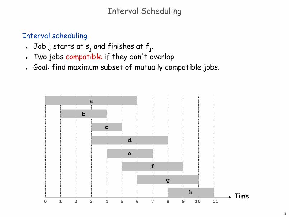
Interval scheduling. Job j starts at sj and finishes at fj. Two jobs compatible if they don't overlap. Goal: find maximum subset of mutually compatible jobs.

Time0 1 2 3 4 5 6 7 8 9 10 11

f

g

h

e

a

b

c

d

3

Interval Scheduling: Greedy Algorithms

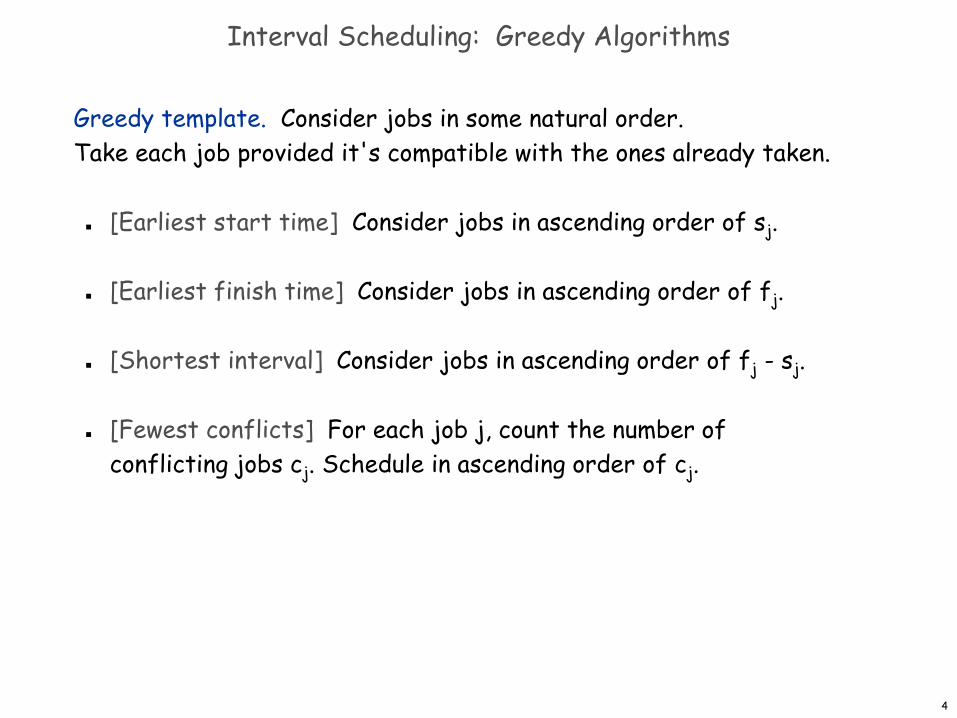
Greedy template. Consider jobs in some natural order.Take each job provided it's compatible with the ones already taken.

[Earliest start time] Consider jobs in ascending order of sj.

[Earliest finish time] Consider jobs in ascending order of fj.

[Shortest interval] Consider jobs in ascending order of fj - sj.

[Fewest conflicts] For each job j, count the number ofconflicting jobs cj. Schedule in ascending order of cj.

4

Interval Scheduling: Greedy Algorithms

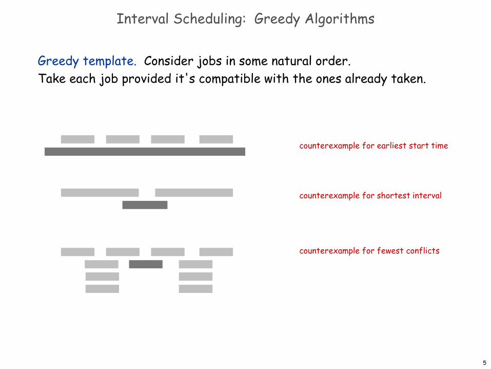
Greedy template. Consider jobs in some natural order.Take each job provided it's compatible with the ones already taken.

counterexample for earliest start time

counterexample for shortest interval

counterexample for fewest conflicts

5

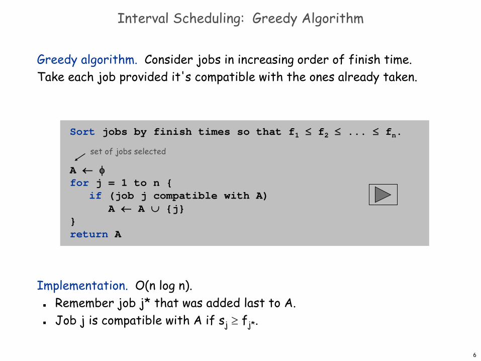
Greedy algorithm. Consider jobs in increasing order of finish time. Take each job provided it's compatible with the ones already taken.

Implementation. O(n log n). Remember job j* that was added last to A. Job j is compatible with A if sj ≥ fj*.

Sort jobs by finish times so that f1 ≤ f2 ≤ ... ≤ fn.

A ← φfor j = 1 to n {

if (job j compatible with A)A ← A ∪ {j}

}return A

set of jobs selected

Interval Scheduling: Greedy Algorithm

6

Interval Scheduling: Analysis

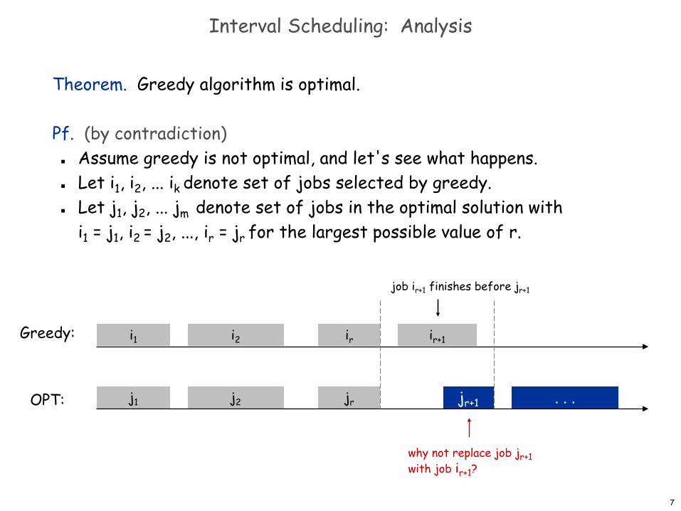
Theorem. Greedy algorithm is optimal.

Pf. (by contradiction) Assume greedy is not optimal, and let's see what happens. Let i1, i2, ... ik denote set of jobs selected by greedy. Let j1, j2, ... jm denote set of jobs in the optimal solution with

i1 = j1, i2 = j2, ..., ir = jr for the largest possible value of r.

j1 j2 jr

i1 i2 ir ir+1

. . .

Greedy:

OPT: jr+1

why not replace job jr+1with job ir+1?

job ir+1 finishes before jr+1

7

j1 j2 jr

i1 i2 ir ir+1

Interval Scheduling: Analysis

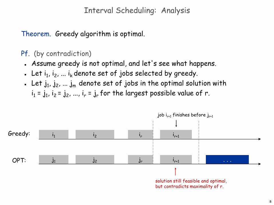
Theorem. Greedy algorithm is optimal.

Pf. (by contradiction) Assume greedy is not optimal, and let's see what happens. Let i1, i2, ... ik denote set of jobs selected by greedy. Let j1, j2, ... jm denote set of jobs in the optimal solution with

i1 = j1, i2 = j2, ..., ir = jr for the largest possible value of r.

. . .

Greedy:

OPT:

solution still feasible and optimal, but contradicts maximality of r.

ir+1

job ir+1 finishes before jr+1

8

Interval Partitioning

Interval Partitioning

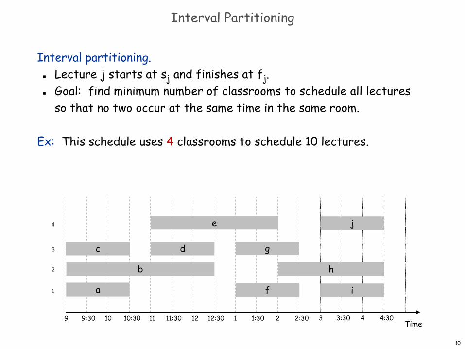
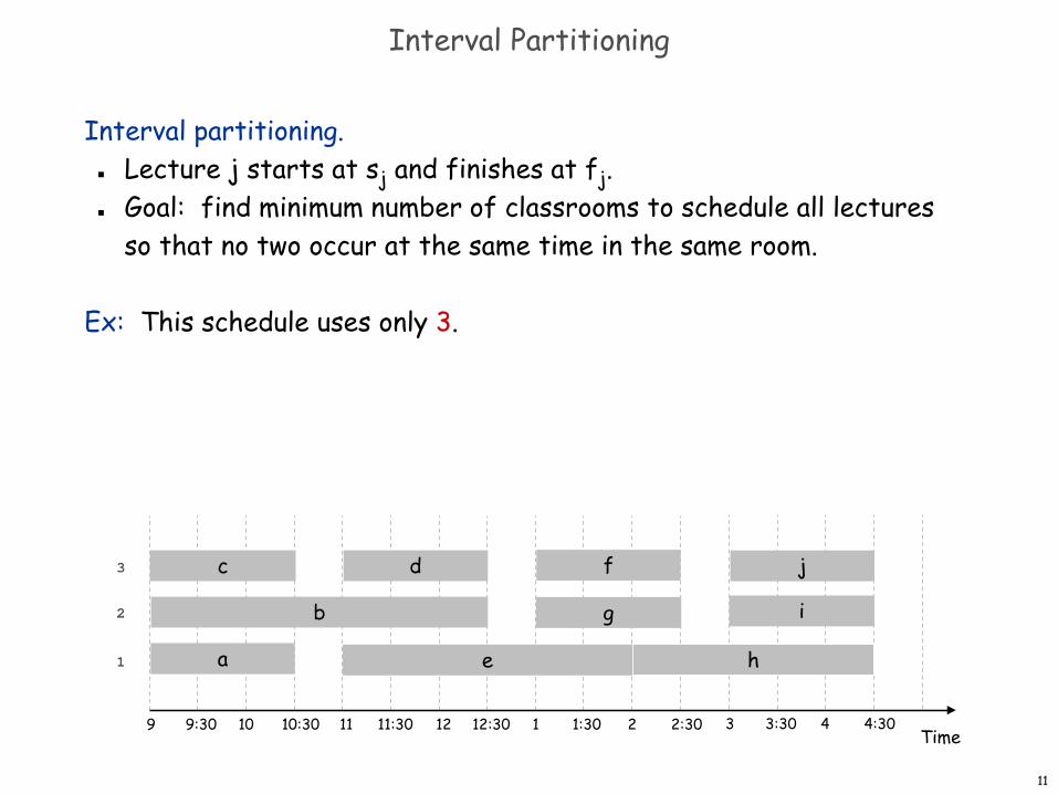
Interval partitioning. Lecture j starts at sj and finishes at fj. Goal: find minimum number of classrooms to schedule all lectures

so that no two occur at the same time in the same room.

Ex: This schedule uses 4 classrooms to schedule 10 lectures.

Time9 9:30 10 10:30 11 11:30 12 12:30 1 1:30 2 2:30

h

c

b

a

e

d g

f i

j

3 3:30 4 4:30

1

2

3

4

10

Interval Partitioning

Interval partitioning. Lecture j starts at sj and finishes at fj. Goal: find minimum number of classrooms to schedule all lectures

so that no two occur at the same time in the same room.

Ex: This schedule uses only 3.

Time9 9:30 10 10:30 11 11:30 12 12:30 1 1:30 2 2:30

h

c

a e

f

g i

j

3 3:30 4 4:30

d

b

1

2

3

11

Interval Partitioning: Lower Bound on Optimal Solution

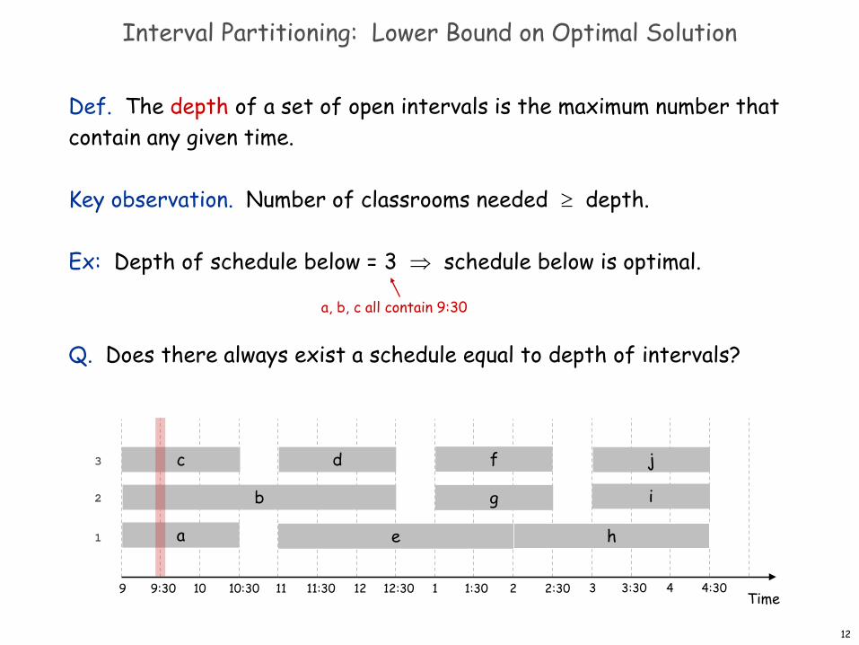
Def. The depth of a set of open intervals is the maximum number that contain any given time.

Key observation. Number of classrooms needed ≥ depth.

Ex: Depth of schedule below = 3 ⇒ schedule below is optimal.

Q. Does there always exist a schedule equal to depth of intervals?

Time9 9:30 10 10:30 11 11:30 12 12:30 1 1:30 2 2:30

h

c

a e

f

g i

j

3 3:30 4 4:30

d

b

a, b, c all contain 9:30

1

2

3

12

Interval Partitioning: Greedy Algorithm

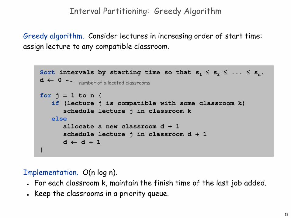
Greedy algorithm. Consider lectures in increasing order of start time: assign lecture to any compatible classroom.

Implementation. O(n log n). For each classroom k, maintain the finish time of the last job added. Keep the classrooms in a priority queue.

Sort intervals by starting time so that s1 ≤ s2 ≤ ... ≤ sn.d ← 0

for j = 1 to n {if (lecture j is compatible with some classroom k)

schedule lecture j in classroom kelse

allocate a new classroom d + 1schedule lecture j in classroom d + 1d ← d + 1

}

number of allocated classrooms

13

Interval Partitioning: Greedy Analysis

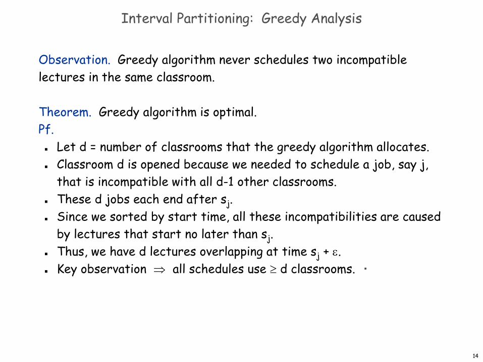
Observation. Greedy algorithm never schedules two incompatible lectures in the same classroom.

Theorem. Greedy algorithm is optimal.Pf. Let d = number of classrooms that the greedy algorithm allocates. Classroom d is opened because we needed to schedule a job, say j,

that is incompatible with all d-1 other classrooms. These d jobs each end after sj. Since we sorted by start time, all these incompatibilities are caused

by lectures that start no later than sj. Thus, we have d lectures overlapping at time sj + ε. Key observation ⇒ all schedules use ≥ d classrooms. ▪

14

Scheduling to Minimize Lateness

Scheduling to Minimizing Lateness

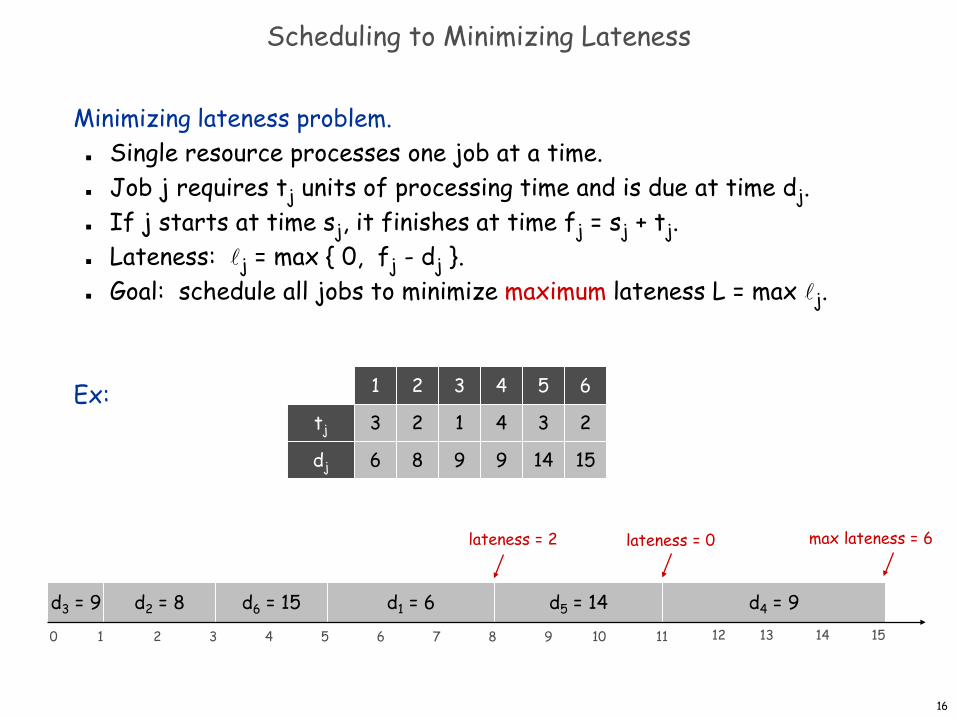
Minimizing lateness problem. Single resource processes one job at a time. Job j requires tj units of processing time and is due at time dj. If j starts at time sj, it finishes at time fj = sj + tj. Lateness: j = max { 0, fj - dj }. Goal: schedule all jobs to minimize maximum lateness L = max j.

Ex:

0 1 2 3 4 5 6 7 8 9 10 11 12 13 14 15

d5 = 14d2 = 8 d6 = 15 d1 = 6 d4 = 9d3 = 9

lateness = 0lateness = 2

dj 6

tj 3

1

8

2

2

9

1

3

9

4

4

14

3

5

15

2

6

max lateness = 6

16

Minimizing Lateness: Greedy Algorithms

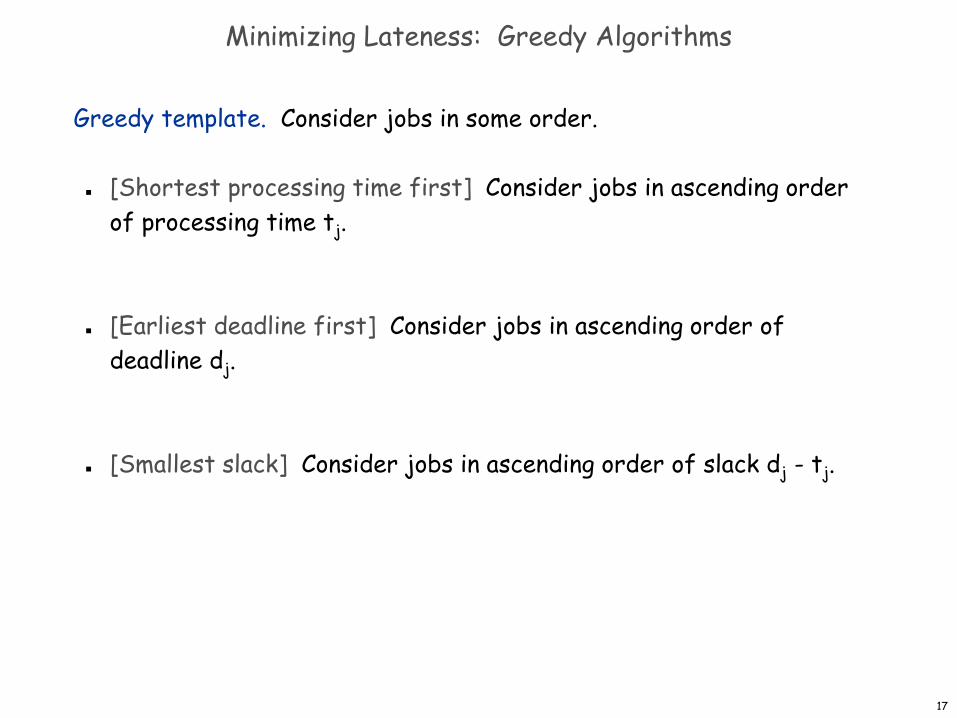
Greedy template. Consider jobs in some order.

[Shortest processing time first] Consider jobs in ascending order of processing time tj.

[Earliest deadline first] Consider jobs in ascending order of deadline dj.

[Smallest slack] Consider jobs in ascending order of slack dj - tj.

17

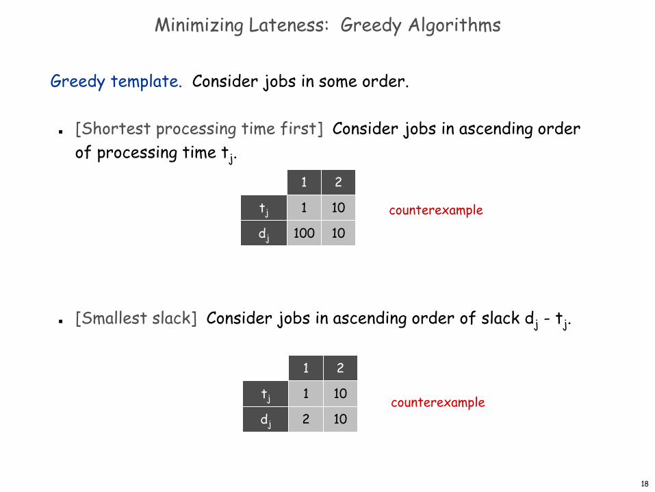
Greedy template. Consider jobs in some order.

[Shortest processing time first] Consider jobs in ascending order of processing time tj.

[Smallest slack] Consider jobs in ascending order of slack dj - tj.

counterexample

counterexample

dj

tj

100

1

1

10

10

2

dj

tj

2

1

1

10

10

2

Minimizing Lateness: Greedy Algorithms

18

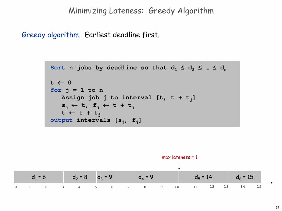
0 1 2 3 4 5 6 7 8 9 10 11 12 13 14 15

d5 = 14d2 = 8 d6 = 15d1 = 6 d4 = 9d3 = 9

max lateness = 1

Sort n jobs by deadline so that d1 ≤ d2 ≤ … ≤ dn

t ← 0for j = 1 to n

Assign job j to interval [t, t + tj]sj ← t, fj ← t + tjt ← t + tj

output intervals [sj, fj]

Minimizing Lateness: Greedy Algorithm

Greedy algorithm. Earliest deadline first.

19

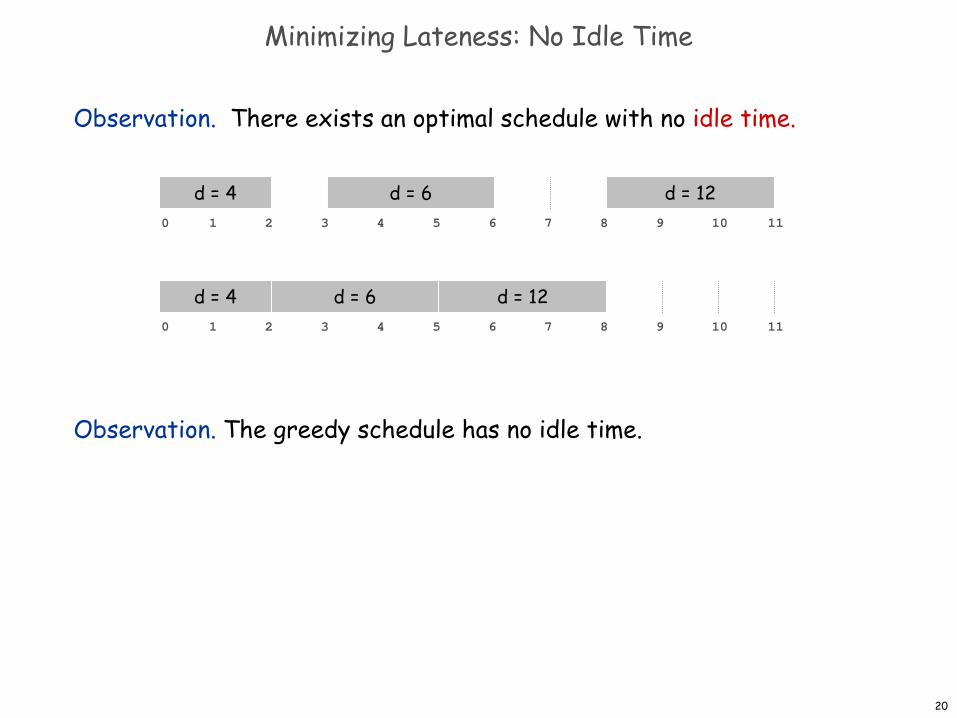
Minimizing Lateness: No Idle Time

Observation. There exists an optimal schedule with no idle time.

Observation. The greedy schedule has no idle time.

0 1 2 3 4 5 6

d = 4 d = 67 8 9 10 11

d = 12

0 1 2 3 4 5 6

d = 4 d = 67 8 9 10 11

d = 12

20

Minimizing Lateness: Inversions

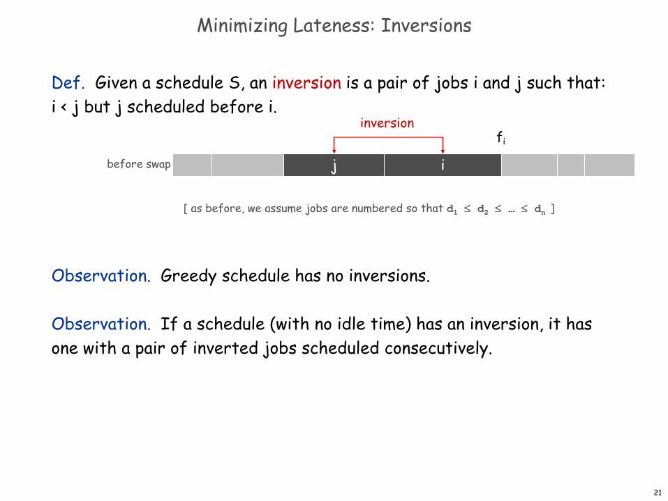
Def. Given a schedule S, an inversion is a pair of jobs i and j such that:i < j but j scheduled before i.

Observation. Greedy schedule has no inversions.

Observation. If a schedule (with no idle time) has an inversion, it has one with a pair of inverted jobs scheduled consecutively.

ijbefore swap

fi

inversion

[ as before, we assume jobs are numbered so that d1 ≤ d2 ≤ … ≤ dn ]

21

Minimizing Lateness: Inversions

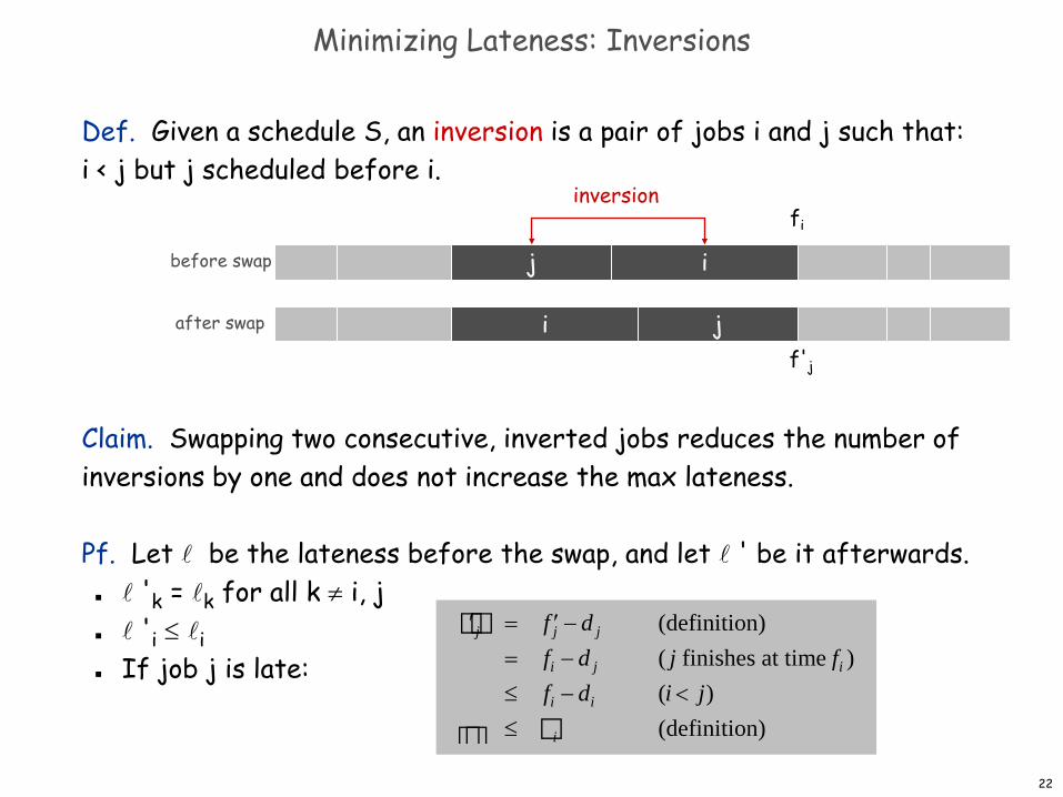
Def. Given a schedule S, an inversion is a pair of jobs i and j such that:i < j but j scheduled before i.

Claim. Swapping two consecutive, inverted jobs reduces the number of inversions by one and does not increase the max lateness.

Pf. Let be the lateness before the swap, and let ' be it afterwards. 'k = k for all k ≠ i, j 'i ≤ i If job j is late:

ij

i j

before swap

after swap

′ j = ′ f j − d j (definition)= fi − d j ( j finishes at time fi )≤ fi − di (i < j)≤ i (definition)

f'j

fi

inversion

22

Minimizing Lateness: Analysis of Greedy Algorithm

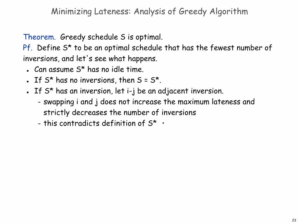
Theorem. Greedy schedule S is optimal.Pf. Define S* to be an optimal schedule that has the fewest number of inversions, and let's see what happens. Can assume S* has no idle time. If S* has no inversions, then S = S*. If S* has an inversion, let i-j be an adjacent inversion.

– swapping i and j does not increase the maximum lateness and strictly decreases the number of inversions

– this contradicts definition of S* ▪

23

Greedy Analysis Strategies

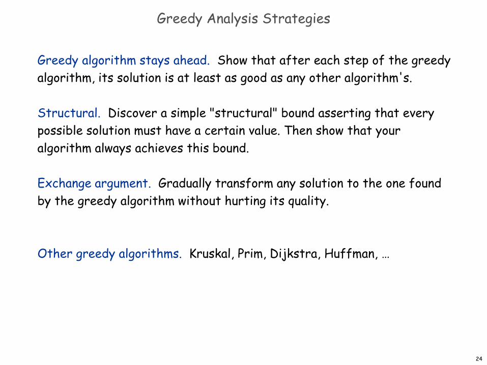
Greedy algorithm stays ahead. Show that after each step of the greedy algorithm, its solution is at least as good as any other algorithm's.

Structural. Discover a simple "structural" bound asserting that every possible solution must have a certain value. Then show that your algorithm always achieves this bound.

Exchange argument. Gradually transform any solution to the one found by the greedy algorithm without hurting its quality.

Other greedy algorithms. Kruskal, Prim, Dijkstra, Huffman, …

24

Optimal Caching

Optimal Offline Caching

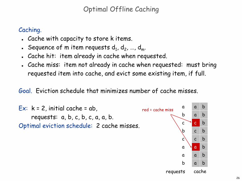
Caching. Cache with capacity to store k items. Sequence of m item requests d1, d2, …, dm. Cache hit: item already in cache when requested. Cache miss: item not already in cache when requested: must bring

requested item into cache, and evict some existing item, if full.

Goal. Eviction schedule that minimizes number of cache misses.

Ex: k = 2, initial cache = ab,requests: a, b, c, b, c, a, a, b.

Optimal eviction schedule: 2 cache misses.

a ba bc bc bc ba b

abcbca

a baa bb

cacherequests

red = cache miss

26

Optimal Offline Caching: Farthest-In-Future

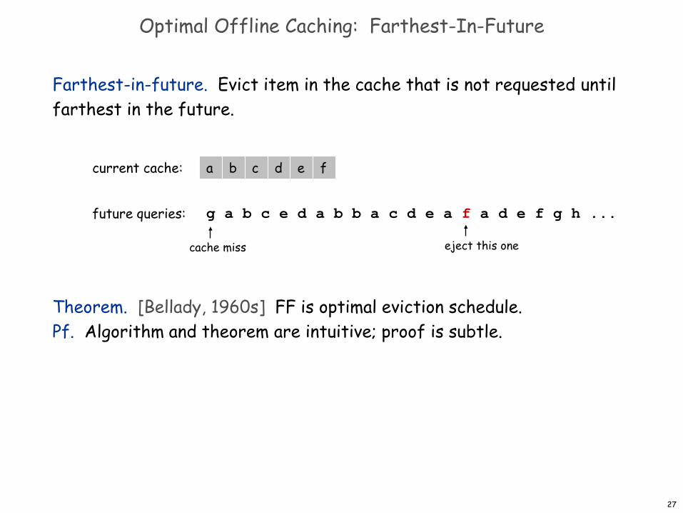
Farthest-in-future. Evict item in the cache that is not requested until farthest in the future.

Theorem. [Bellady, 1960s] FF is optimal eviction schedule.Pf. Algorithm and theorem are intuitive; proof is subtle.

a b

g a b c e d a b b a c d e a f a d e f g h ...

current cache: c d e f

future queries:

cache miss eject this one

27

Reduced Eviction Schedules

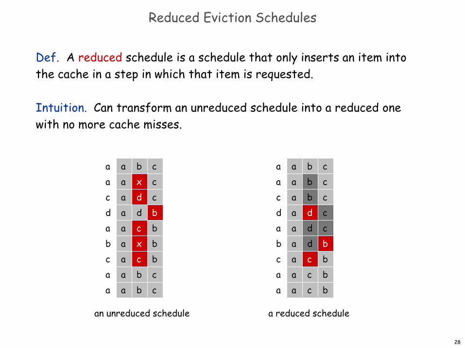
Def. A reduced schedule is a schedule that only inserts an item into the cache in a step in which that item is requested.

Intuition. Can transform an unreduced schedule into a reduced one with no more cache misses.

a x

an unreduced schedule

ca d ca d ba c ba x ba c ba b ca b c

acdabcaa

a b

a reduced schedule

ca b ca d ca d ca d ba c ba c ba c b

acdabcaa

a b ca a b ca

28

Reduced Eviction Schedules

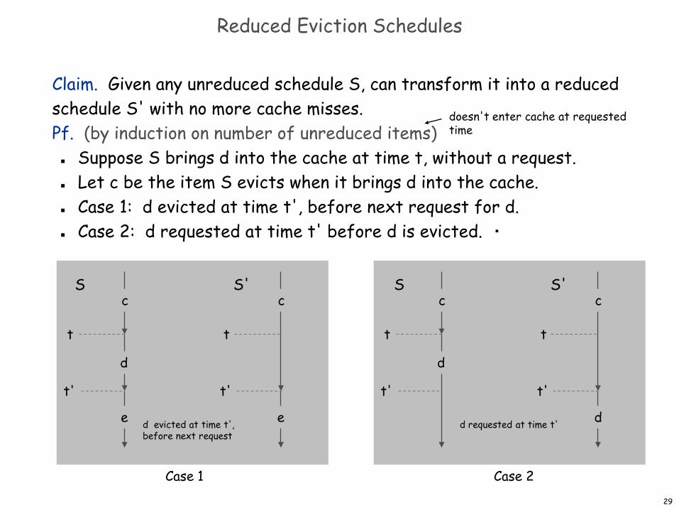
Claim. Given any unreduced schedule S, can transform it into a reduced schedule S' with no more cache misses.Pf. (by induction on number of unreduced items) Suppose S brings d into the cache at time t, without a request. Let c be the item S evicts when it brings d into the cache. Case 1: d evicted at time t', before next request for d. Case 2: d requested at time t' before d is evicted. ▪

t

t'

d

c

t

t'

cS'

d

S

d requested at time t'

t

t'

d

c

t

t'

cS'

e

S

d evicted at time t',before next request

e

doesn't enter cache at requested time

Case 1 Case 229

Farthest-In-Future: Analysis

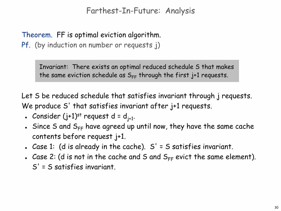
Theorem. FF is optimal eviction algorithm.Pf. (by induction on number or requests j)

Let S be reduced schedule that satisfies invariant through j requests. We produce S' that satisfies invariant after j+1 requests. Consider (j+1)st request d = dj+1. Since S and SFF have agreed up until now, they have the same cache

contents before request j+1. Case 1: (d is already in the cache). S' = S satisfies invariant. Case 2: (d is not in the cache and S and SFF evict the same element).

S' = S satisfies invariant.

Invariant: There exists an optimal reduced schedule S that makes the same eviction schedule as SFF through the first j+1 requests.

30

j

Farthest-In-Future: Analysis

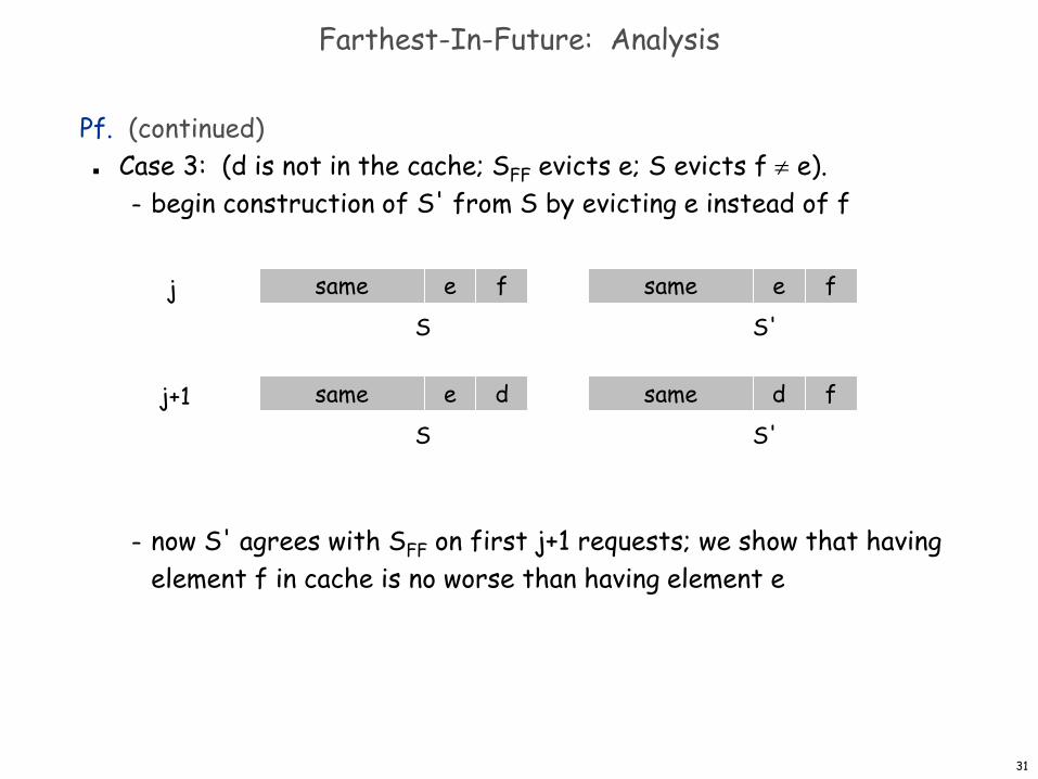
Pf. (continued) Case 3: (d is not in the cache; SFF evicts e; S evicts f ≠ e).

– begin construction of S' from S by evicting e instead of f

– now S' agrees with SFF on first j+1 requests; we show that having element f in cache is no worse than having element e

same f same fee

S S'

j same d same fde

S S'j+1

31

Farthest-In-Future: Analysis

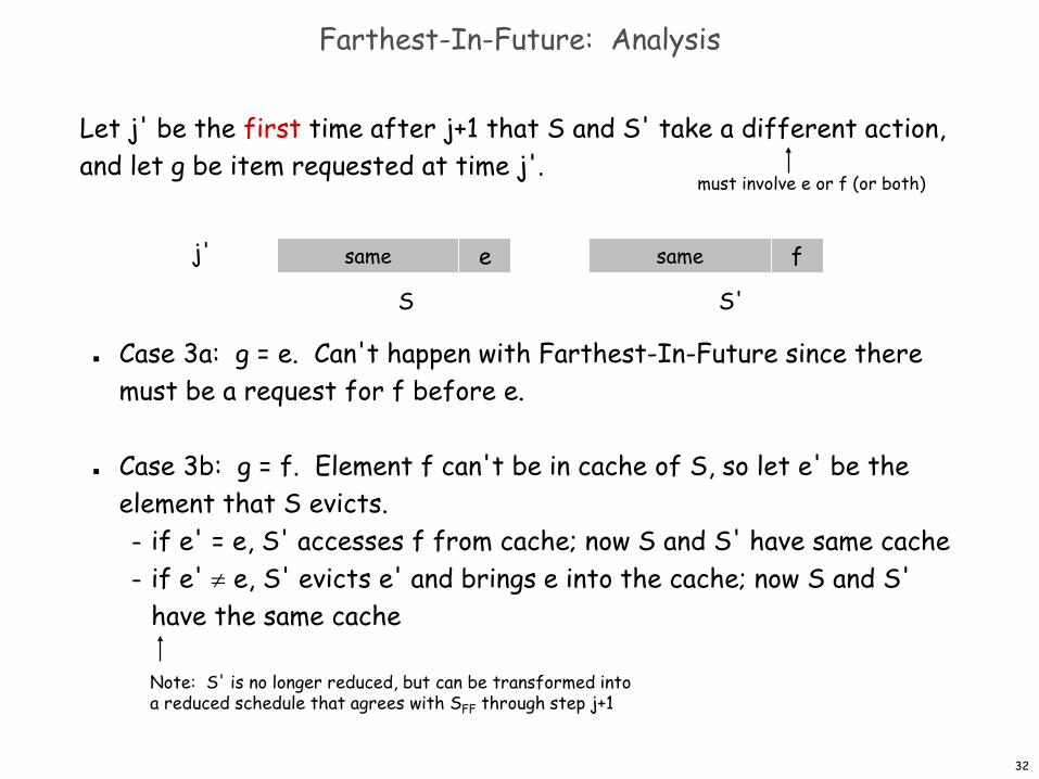
Let j' be the first time after j+1 that S and S' take a different action, and let g be item requested at time j'.

Case 3a: g = e. Can't happen with Farthest-In-Future since there must be a request for f before e.

Case 3b: g = f. Element f can't be in cache of S, so let e' be the element that S evicts.

– if e' = e, S' accesses f from cache; now S and S' have same cache– if e' ≠ e, S' evicts e' and brings e into the cache; now S and S'

have the same cache

same e same f

S S'

j'

Note: S' is no longer reduced, but can be transformed intoa reduced schedule that agrees with SFF through step j+1

must involve e or f (or both)

32

Farthest-In-Future: Analysis

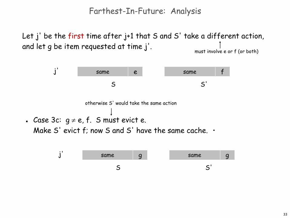
Let j' be the first time after j+1 that S and S' take a different action, and let g be item requested at time j'.

Case 3c: g ≠ e, f. S must evict e.Make S' evict f; now S and S' have the same cache. ▪

same g same g

S S'

j'

otherwise S' would take the same action

same e same f

S S'

j'

must involve e or f (or both)

33

Caching Perspective

Online vs. offline algorithms. Offline: full sequence of requests is known a priori. Online (reality): requests are not known in advance. Caching is among most fundamental online problems in CS.

LIFO. Evict page brought in most recently.LRU. Evict page whose most recent access was earliest.

Theorem. FF is optimal offline eviction algorithm. Provides basis for understanding and analyzing online algorithms. LRU is k-competitive. [Section 13.8] LIFO is arbitrarily bad.

FF with direction of time reversed!

34

Selecting Breakpoints

Selecting Breakpoints

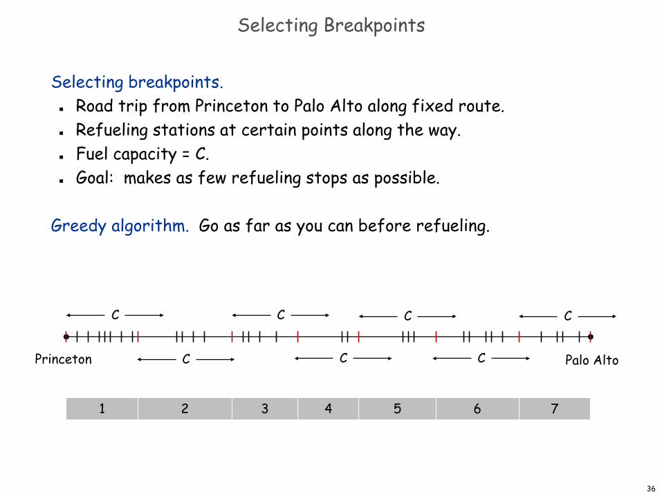
Selecting breakpoints. Road trip from Princeton to Palo Alto along fixed route. Refueling stations at certain points along the way. Fuel capacity = C. Goal: makes as few refueling stops as possible.

Greedy algorithm. Go as far as you can before refueling.

Princeton Palo Alto

1

C

C

2

C

3

C

4

C

5

C

6

C

7

36

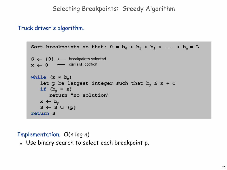
Truck driver's algorithm.

Implementation. O(n log n) Use binary search to select each breakpoint p.

Selecting Breakpoints: Greedy Algorithm

Sort breakpoints so that: 0 = b0 < b1 < b2 < ... < bn = L

S ← {0}x ← 0

while (x ≠ bn)let p be largest integer such that bp ≤ x + Cif (bp = x)

return "no solution"x ← bpS ← S ∪ {p}

return S

breakpoints selectedcurrent location

37

Selecting Breakpoints: Correctness

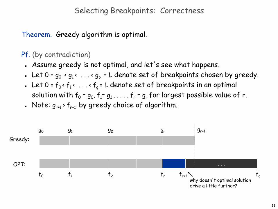
Theorem. Greedy algorithm is optimal.

Pf. (by contradiction) Assume greedy is not optimal, and let's see what happens. Let 0 = g0 < g1 < . . . < gp = L denote set of breakpoints chosen by greedy. Let 0 = f0 < f1 < . . . < fq = L denote set of breakpoints in an optimal

solution with f0 = g0, f1= g1 , . . . , fr = gr for largest possible value of r. Note: gr+1 > fr+1 by greedy choice of algorithm.

. . .

Greedy:

OPT:

g0 g1 g2

f0 f1 f2 fq

gr

frwhy doesn't optimal solution drive a little further?

gr+1

fr+1

38

Selecting Breakpoints: Correctness

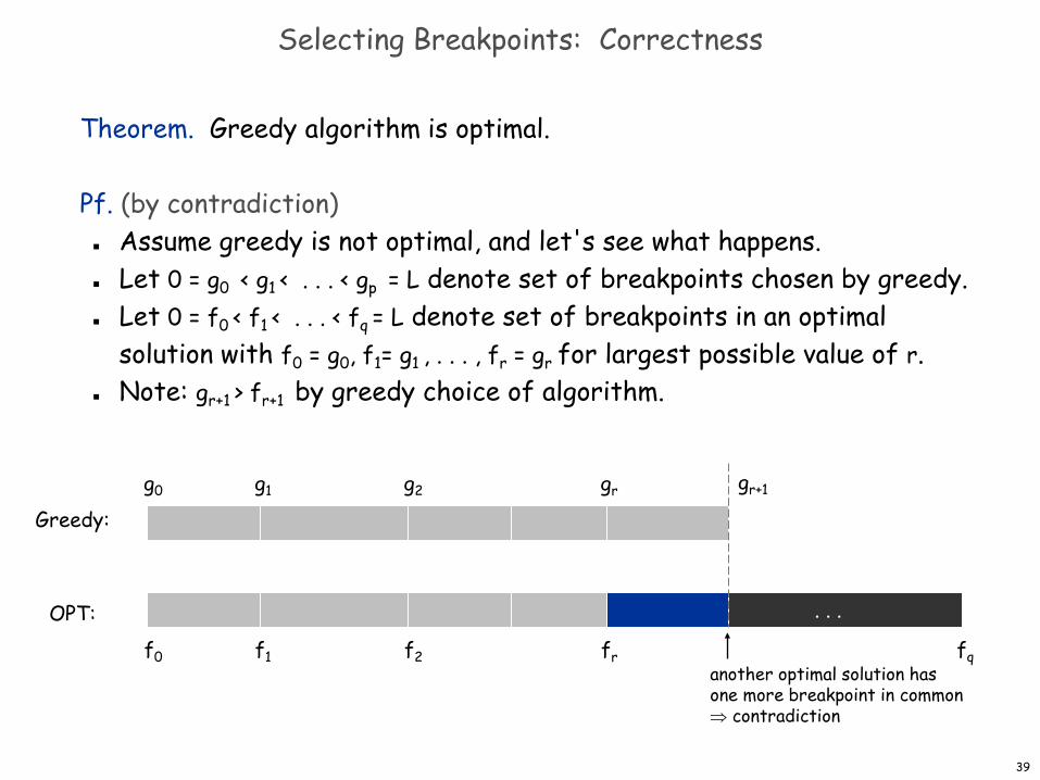
Theorem. Greedy algorithm is optimal.

Pf. (by contradiction) Assume greedy is not optimal, and let's see what happens. Let 0 = g0 < g1 < . . . < gp = L denote set of breakpoints chosen by greedy. Let 0 = f0 < f1 < . . . < fq = L denote set of breakpoints in an optimal

solution with f0 = g0, f1= g1 , . . . , fr = gr for largest possible value of r. Note: gr+1 > fr+1 by greedy choice of algorithm.

another optimal solution hasone more breakpoint in common⇒ contradiction

. . .

Greedy:

OPT:

g0 g1 g2

f0 f1 f2 fq

gr

fr

gr+1

39

Coin Changing

Coin Changing

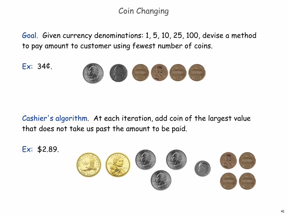
Goal. Given currency denominations: 1, 5, 10, 25, 100, devise a method to pay amount to customer using fewest number of coins.

Ex: 34¢.

Cashier's algorithm. At each iteration, add coin of the largest value that does not take us past the amount to be paid.

Ex: $2.89.

41

Coin-Changing: Greedy Algorithm

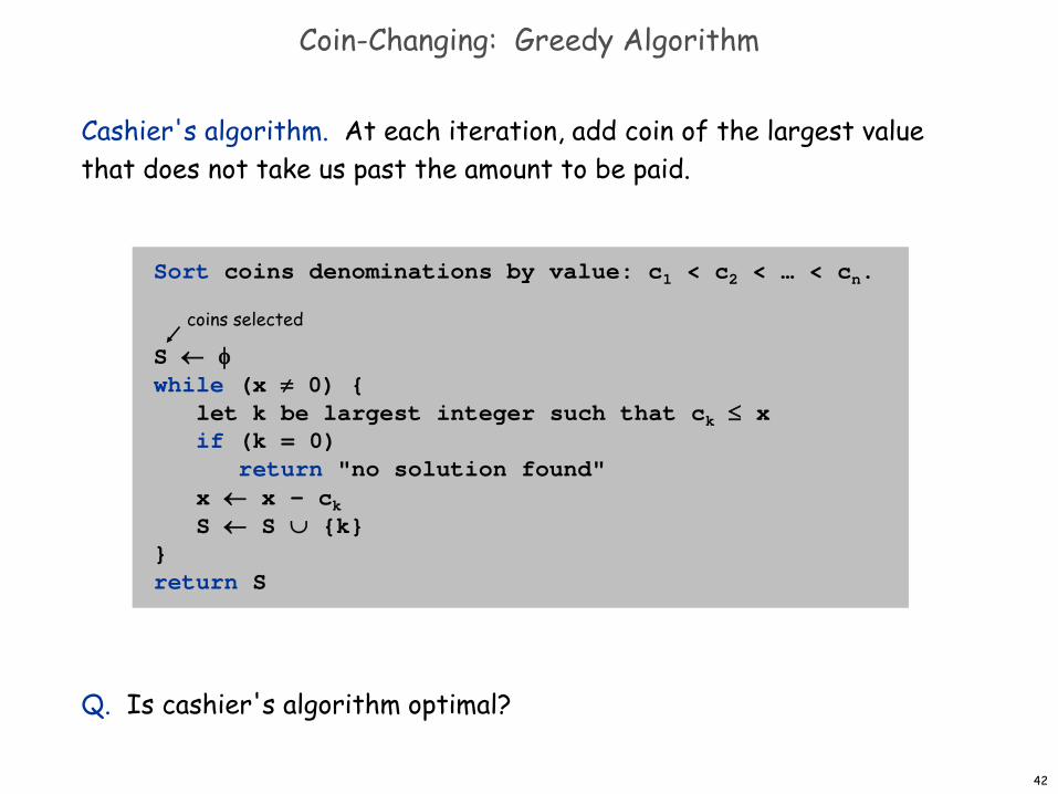
Cashier's algorithm. At each iteration, add coin of the largest value that does not take us past the amount to be paid.

Q. Is cashier's algorithm optimal?

Sort coins denominations by value: c1 < c2 < … < cn.

S ← φwhile (x ≠ 0) {

let k be largest integer such that ck ≤ xif (k = 0)

return "no solution found"x ← x - ckS ← S ∪ {k}

}return S

coins selected

42

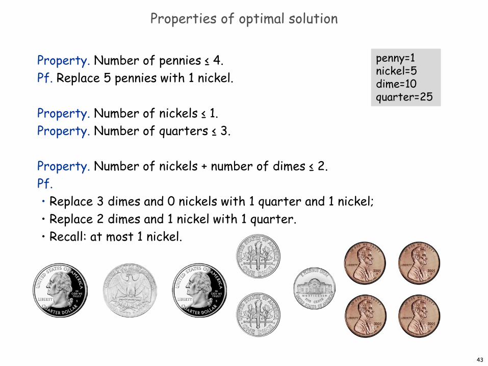
Properties of optimal solution

Property. Number of pennies ≤ 4.Pf. Replace 5 pennies with 1 nickel.

Property. Number of nickels ≤ 1.Property. Number of quarters ≤ 3.

Property. Number of nickels + number of dimes ≤ 2.Pf.・Replace 3 dimes and 0 nickels with 1 quarter and 1 nickel;・Replace 2 dimes and 1 nickel with 1 quarter.・Recall: at most 1 nickel.

penny=1nickel=5dime=10quarter=25

43

Coin-Changing: Analysis of Greedy Algorithm

Theorem. Greedy algorithm is optimal for U.S. coinage: 1, 5, 10, 25, 100.Pf. (by induction on x) Consider optimal way to change ck ≤ x < ck+1 : greedy takes coin k. We claim that any optimal solution must also take coin k.

– if not, it needs enough coins of type c1, …, ck-1 to add up to x– table below indicates no optimal solution can do this

Problem reduces to coin-changing x - ck cents, which, by induction, is optimally solved by greedy algorithm. ▪

1

ck

10

25

100

P ≤ 4

All optimal solutionsmust satisfy

N + D ≤ 2

Q ≤ 3

5 N ≤ 1

no limit

k

1

3

4

5

2

-

Max value of coins1, 2, …, k-1 in any OPT

4 + 5 = 9

20 + 4 = 24

4

75 + 24 = 99

44

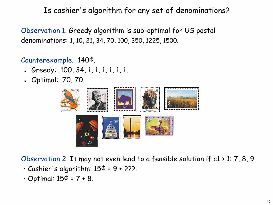
Is cashier's algorithm for any set of denominations?

Observation 1. Greedy algorithm is sub-optimal for US postal denominations: 1, 10, 21, 34, 70, 100, 350, 1225, 1500.

Counterexample. 140¢. Greedy: 100, 34, 1, 1, 1, 1, 1, 1. Optimal: 70, 70.

Observation 2. It may not even lead to a feasible solution if c1 > 1: 7, 8, 9.・Cashier's algorithm: 15¢ = 9 + ???.・Optimal: 15¢ = 7 + 8.

45

Minimum Spanning Tree

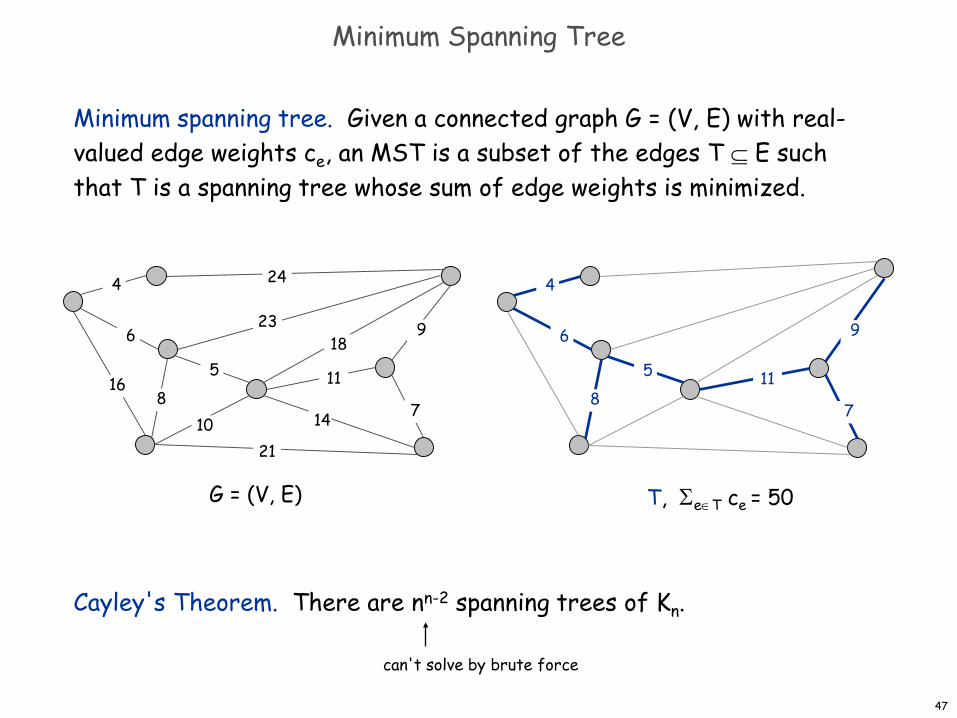
Minimum Spanning Tree

Minimum spanning tree. Given a connected graph G = (V, E) with real-valued edge weights ce, an MST is a subset of the edges T ⊆ E such that T is a spanning tree whose sum of edge weights is minimized.

Cayley's Theorem. There are nn-2 spanning trees of Kn.

5

23

10 21

14

24

16

6

4

189

7

118

5

6

4

9

7

118

G = (V, E) T, Σe∈T ce = 50

can't solve by brute force

47

Applications

MST is fundamental problem with diverse applications.

Network design.– telephone, electrical, hydraulic, TV cable, computer, road

Approximation algorithms for NP-hard problems.– traveling salesperson problem, Steiner tree

Indirect applications.– max bottleneck paths– LDPC codes for error correction– image registration with Renyi entropy– learning salient features for real-time face verification– reducing data storage in sequencing amino acids in a protein– model locality of particle interactions in turbulent fluid flows– autoconfig protocol for Ethernet bridging to avoid cycles in a network

Cluster analysis.

48

Greedy Algorithms

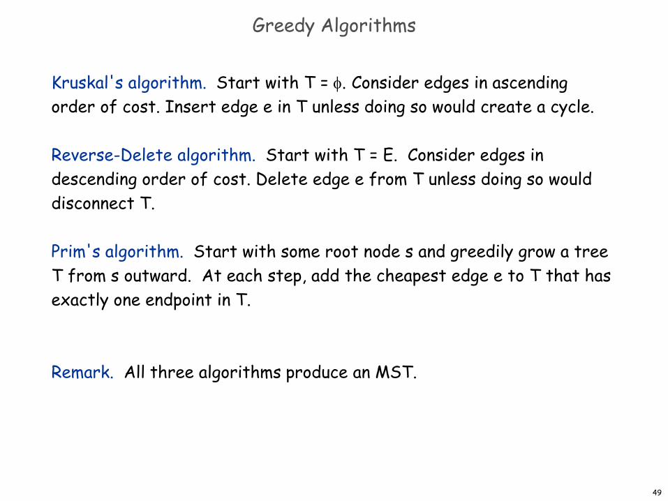
Kruskal's algorithm. Start with T = φ. Consider edges in ascending order of cost. Insert edge e in T unless doing so would create a cycle.

Reverse-Delete algorithm. Start with T = E. Consider edges in descending order of cost. Delete edge e from T unless doing so would disconnect T.

Prim's algorithm. Start with some root node s and greedily grow a tree T from s outward. At each step, add the cheapest edge e to T that has exactly one endpoint in T.

Remark. All three algorithms produce an MST.

49

Greedy Algorithms

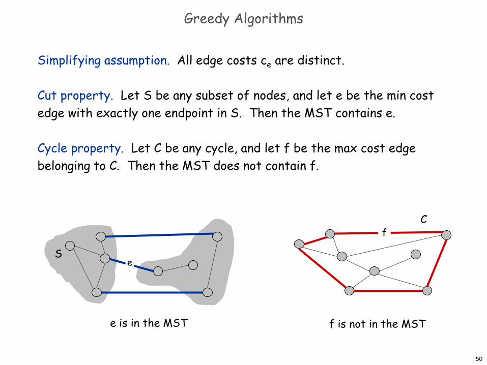
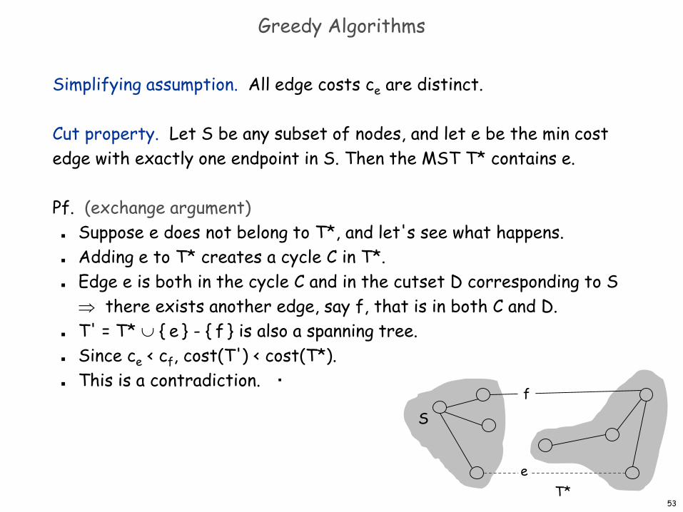
Simplifying assumption. All edge costs ce are distinct.

Cut property. Let S be any subset of nodes, and let e be the min cost edge with exactly one endpoint in S. Then the MST contains e.

Cycle property. Let C be any cycle, and let f be the max cost edge belonging to C. Then the MST does not contain f.

f C

S

e is in the MST

e

f is not in the MST

50

Cycles and Cuts

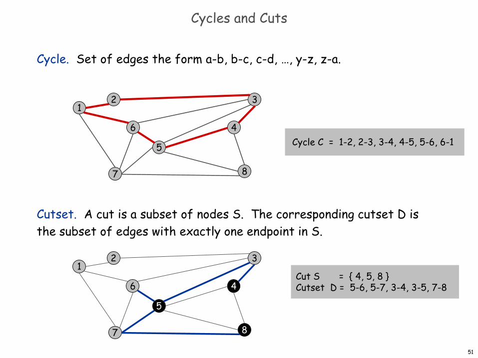
Cycle. Set of edges the form a-b, b-c, c-d, …, y-z, z-a.

Cutset. A cut is a subset of nodes S. The corresponding cutset D is the subset of edges with exactly one endpoint in S.

Cycle C = 1-2, 2-3, 3-4, 4-5, 5-6, 6-1

13

8

2

6

7

4

5

Cut S = { 4, 5, 8 }Cutset D = 5-6, 5-7, 3-4, 3-5, 7-8

13

8

2

6

7

4

5

51

Cycle-Cut Intersection

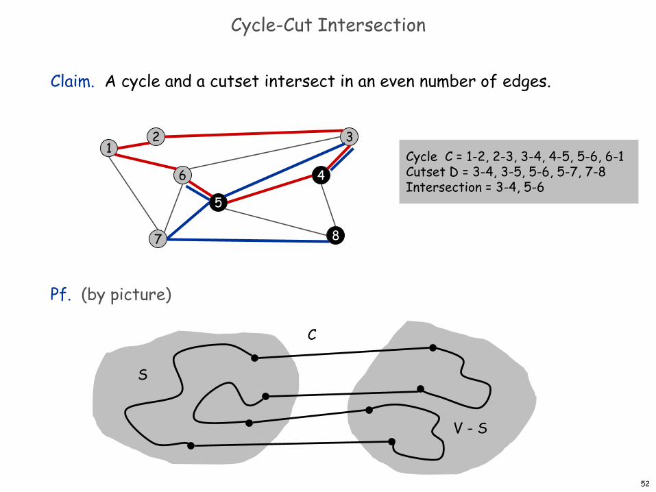
Claim. A cycle and a cutset intersect in an even number of edges.

Pf. (by picture)

13

8

2

6

7

4

5

S

V - S

C

Cycle C = 1-2, 2-3, 3-4, 4-5, 5-6, 6-1Cutset D = 3-4, 3-5, 5-6, 5-7, 7-8 Intersection = 3-4, 5-6

52

Greedy Algorithms

Simplifying assumption. All edge costs ce are distinct.

Cut property. Let S be any subset of nodes, and let e be the min cost edge with exactly one endpoint in S. Then the MST T* contains e.

Pf. (exchange argument) Suppose e does not belong to T*, and let's see what happens. Adding e to T* creates a cycle C in T*. Edge e is both in the cycle C and in the cutset D corresponding to S

⇒ there exists another edge, say f, that is in both C and D. T' = T* ∪ { e } - { f } is also a spanning tree. Since ce < cf, cost(T') < cost(T*). This is a contradiction. ▪

f

T*e

S

53

Greedy Algorithms

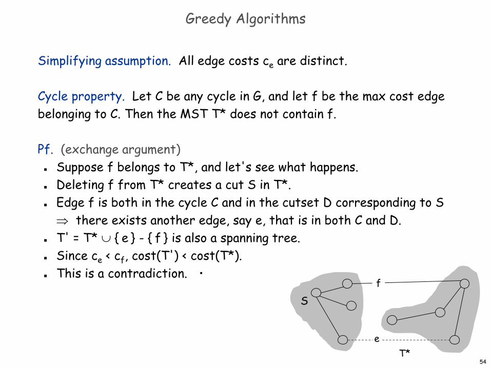
Simplifying assumption. All edge costs ce are distinct.

Cycle property. Let C be any cycle in G, and let f be the max cost edge belonging to C. Then the MST T* does not contain f.

Pf. (exchange argument) Suppose f belongs to T*, and let's see what happens. Deleting f from T* creates a cut S in T*. Edge f is both in the cycle C and in the cutset D corresponding to S

⇒ there exists another edge, say e, that is in both C and D. T' = T* ∪ { e } - { f } is also a spanning tree. Since ce < cf, cost(T') < cost(T*). This is a contradiction. ▪

f

T*e

S

54

Prim's Algorithm: Proof of Correctness

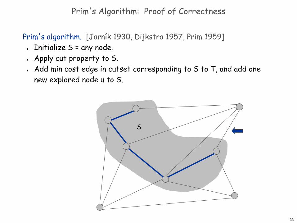
Prim's algorithm. [Jarník 1930, Dijkstra 1957, Prim 1959] Initialize S = any node. Apply cut property to S. Add min cost edge in cutset corresponding to S to T, and add one

new explored node u to S.

S

55

Implementation: Prim's Algorithm

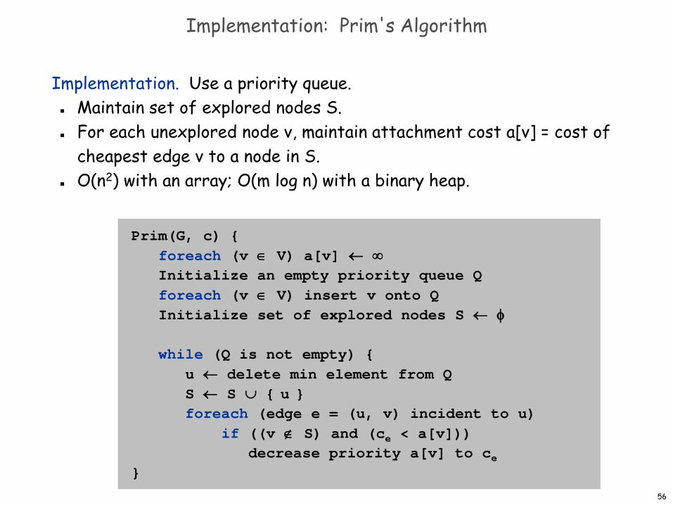
Prim(G, c) {foreach (v ∈ V) a[v] ← ∞Initialize an empty priority queue Qforeach (v ∈ V) insert v onto QInitialize set of explored nodes S ← φ

while (Q is not empty) {u ← delete min element from QS ← S ∪ { u }foreach (edge e = (u, v) incident to u)

if ((v ∉ S) and (ce < a[v]))decrease priority a[v] to ce

}

Implementation. Use a priority queue. Maintain set of explored nodes S. For each unexplored node v, maintain attachment cost a[v] = cost of

cheapest edge v to a node in S. O(n2) with an array; O(m log n) with a binary heap.

56

Kruskal's Algorithm: Proof of Correctness

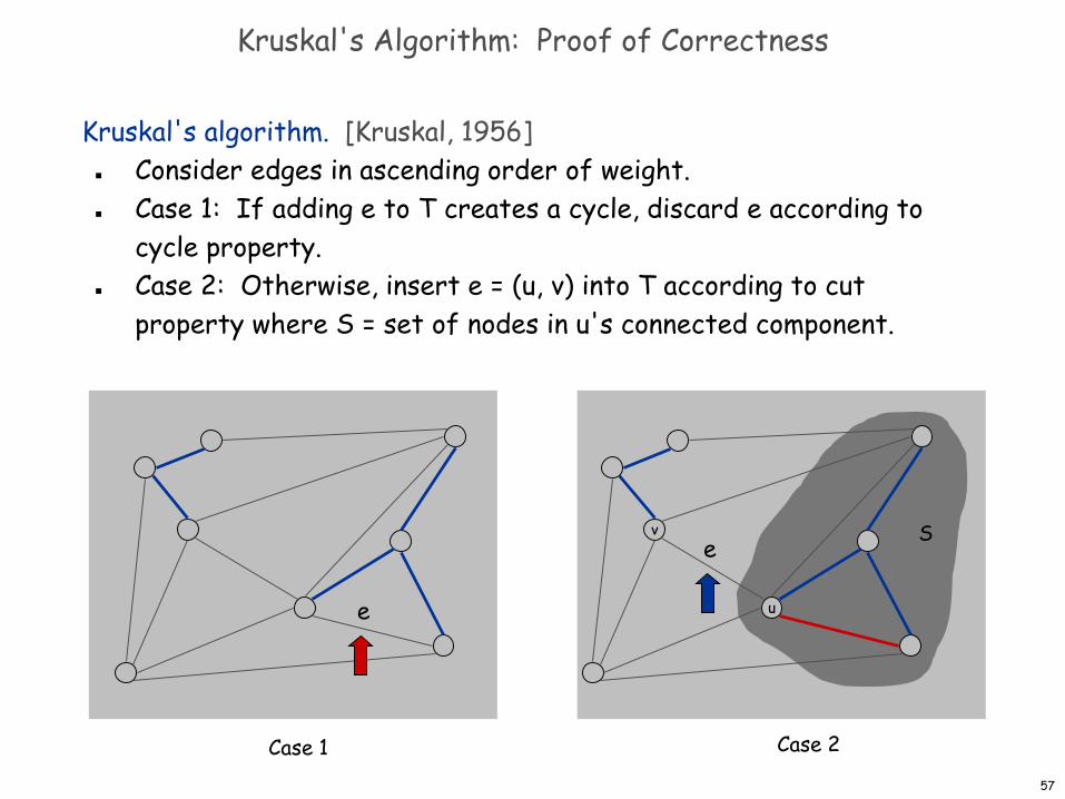
Kruskal's algorithm. [Kruskal, 1956] Consider edges in ascending order of weight. Case 1: If adding e to T creates a cycle, discard e according to

cycle property. Case 2: Otherwise, insert e = (u, v) into T according to cut

property where S = set of nodes in u's connected component.

Case 1

v

u

Case 2

e

e S

57

Implementation: Kruskal's Algorithm

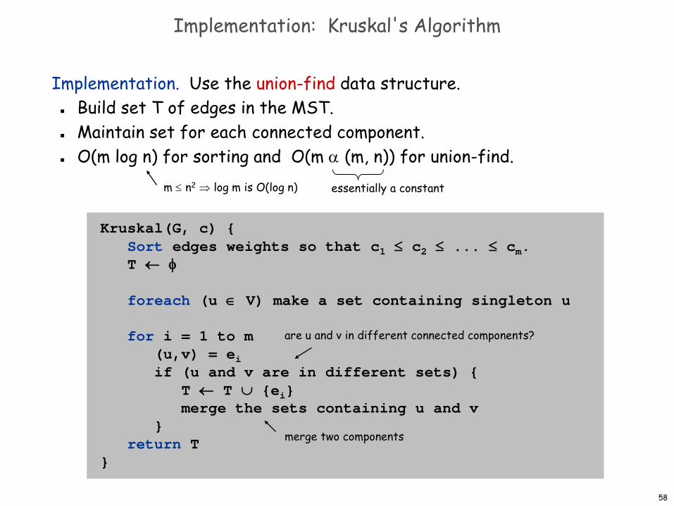
Kruskal(G, c) {Sort edges weights so that c1 ≤ c2 ≤ ... ≤ cm.T ← φ

foreach (u ∈ V) make a set containing singleton u

for i = 1 to m(u,v) = eiif (u and v are in different sets) {

T ← T ∪ {ei}merge the sets containing u and v

}return T

}

Implementation. Use the union-find data structure. Build set T of edges in the MST. Maintain set for each connected component. O(m log n) for sorting and O(m α (m, n)) for union-find.

are u and v in different connected components?

merge two components

m ≤ n2 ⇒ log m is O(log n) essentially a constant

58

Lexicographic Tiebreaking

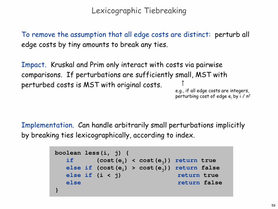
To remove the assumption that all edge costs are distinct: perturb all edge costs by tiny amounts to break any ties.

Impact. Kruskal and Prim only interact with costs via pairwise comparisons. If perturbations are sufficiently small, MST with perturbed costs is MST with original costs.

Implementation. Can handle arbitrarily small perturbations implicitly by breaking ties lexicographically, according to index.

boolean less(i, j) {if (cost(ei) < cost(ej)) return trueelse if (cost(ei) > cost(ej)) return falseelse if (i < j) return trueelse return false

}

e.g., if all edge costs are integers,perturbing cost of edge ei by i / n2

59

MST Algorithms: Theory

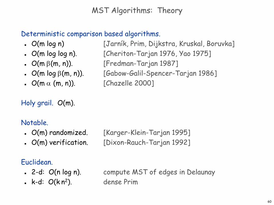
Deterministic comparison based algorithms. O(m log n) [Jarník, Prim, Dijkstra, Kruskal, Boruvka] O(m log log n). [Cheriton-Tarjan 1976, Yao 1975] O(m β(m, n)). [Fredman-Tarjan 1987] O(m log β(m, n)). [Gabow-Galil-Spencer-Tarjan 1986] O(m α (m, n)). [Chazelle 2000]

Holy grail. O(m).

Notable. O(m) randomized. [Karger-Klein-Tarjan 1995] O(m) verification. [Dixon-Rauch-Tarjan 1992]

Euclidean. 2-d: O(n log n). compute MST of edges in Delaunay k-d: O(k n2). dense Prim

60

Clustering

Clustering

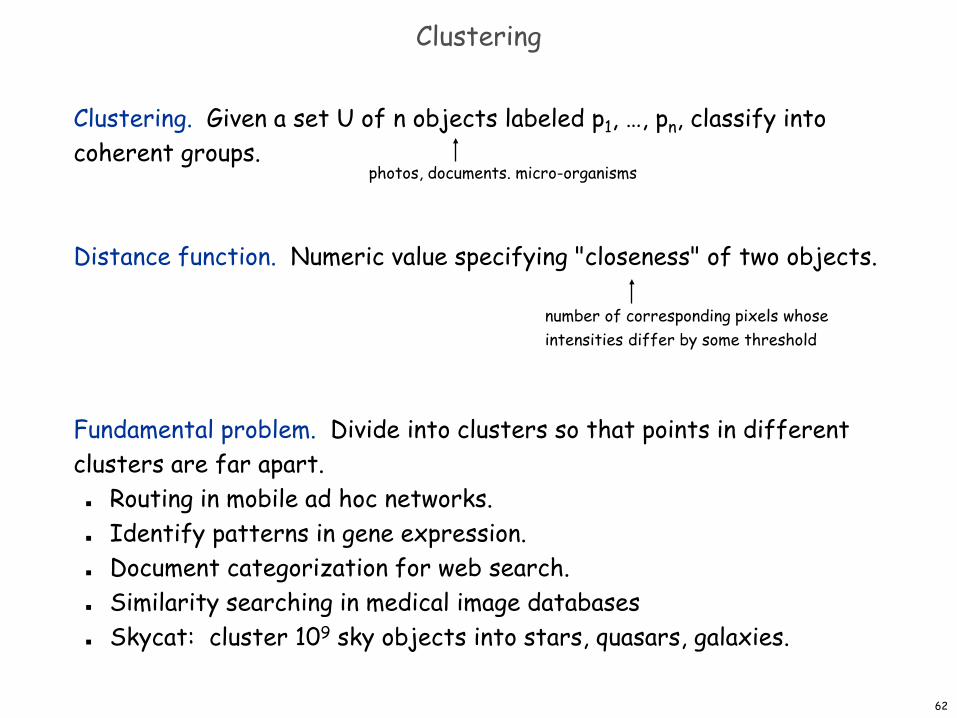
Clustering. Given a set U of n objects labeled p1, …, pn, classify into coherent groups.

Distance function. Numeric value specifying "closeness" of two objects.

Fundamental problem. Divide into clusters so that points in different clusters are far apart. Routing in mobile ad hoc networks. Identify patterns in gene expression. Document categorization for web search. Similarity searching in medical image databases Skycat: cluster 109 sky objects into stars, quasars, galaxies.

photos, documents. micro-organisms

number of corresponding pixels whoseintensities differ by some threshold

62

Clustering of Maximum Spacing

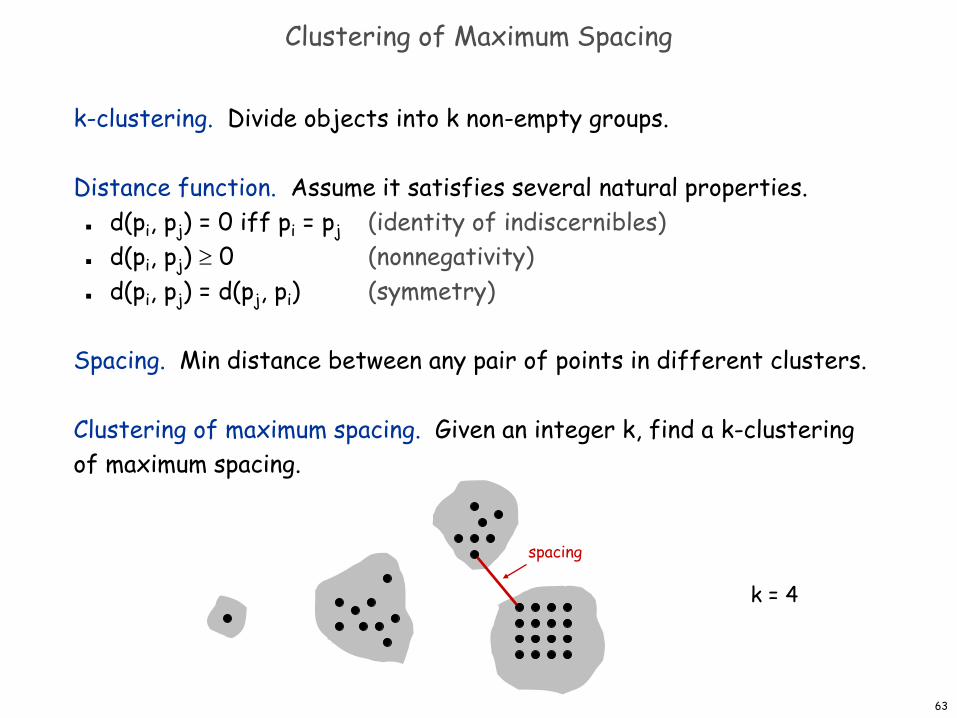
k-clustering. Divide objects into k non-empty groups.

Distance function. Assume it satisfies several natural properties. d(pi, pj) = 0 iff pi = pj (identity of indiscernibles) d(pi, pj) ≥ 0 (nonnegativity) d(pi, pj) = d(pj, pi) (symmetry)

Spacing. Min distance between any pair of points in different clusters.

Clustering of maximum spacing. Given an integer k, find a k-clustering of maximum spacing.

spacing

k = 4

63

Greedy Clustering Algorithm

Single-link k-clustering algorithm. Form a graph on the vertex set U, corresponding to n clusters. Find the closest pair of objects such that each object is in a

different cluster, and add an edge between them. Repeat n-k times until there are exactly k clusters.

Key observation. This procedure is precisely Kruskal's algorithm(except we stop when there are k connected components).

Remark. Equivalent to finding an MST and deleting the k-1 most expensive edges.

64

Greedy Clustering Algorithm: Analysis

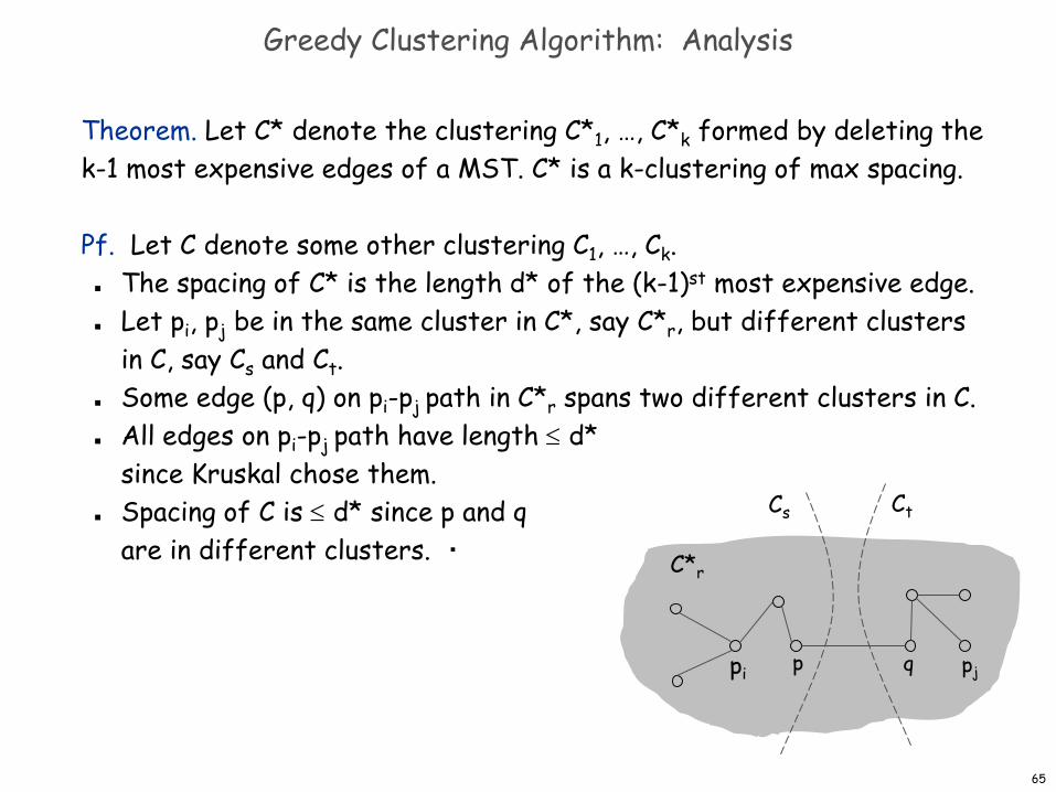
Theorem. Let C* denote the clustering C*1, …, C*k formed by deleting thek-1 most expensive edges of a MST. C* is a k-clustering of max spacing.

Pf. Let C denote some other clustering C1, …, Ck. The spacing of C* is the length d* of the (k-1)st most expensive edge. Let pi, pj be in the same cluster in C*, say C*r, but different clusters

in C, say Cs and Ct. Some edge (p, q) on pi-pj path in C*r spans two different clusters in C. All edges on pi-pj path have length ≤ d*

since Kruskal chose them. Spacing of C is ≤ d* since p and q

are in different clusters. ▪

p qpi pj

Cs Ct

C*r

65

Greed is good.

Greed is right.

Greed works.

Greed clarifies, cuts through, and captures the essence of the evolutionary spirit.

- Gordon Gecko (Michael Douglas)

66