greedy algorithms - dalhousie universitywhidden/csci3110/slides/greedy.pdf · 2019. 5. 21. · the...
TRANSCRIPT

Greedy Algorithms
Textbook Reading
Chapters 16, 17, 21, 23 & 24

Overview
Design principle:
Make progress towards a globally optimal solution by making locally optimal choices,hence the name.
Problems:
• Interval scheduling• Minimum spanning tree• Shortest paths• Minimum-length codes
Proof techniques:
• Induction• The greedy algorithm “stays ahead”• Exchange argument
Data structures:
• Priority queue• Union-find data structure

Interval Scheduling
Given:
A set of activities competing for time intervals on a certain resource(E.g., classes to be scheduled competing for a classroom)
Goal:
Schedule as many non-conflicting activities as possible

Interval Scheduling
Given:
A set of activities competing for time intervals on a certain resource(E.g., classes to be scheduled competing for a classroom)
Goal:
Schedule as many non-conflicting activities as possible

Interval Scheduling
Given:
A set of activities competing for time intervals on a certain resource(E.g., classes to be scheduled competing for a classroom)
Goal:
Schedule as many non-conflicting activities as possible
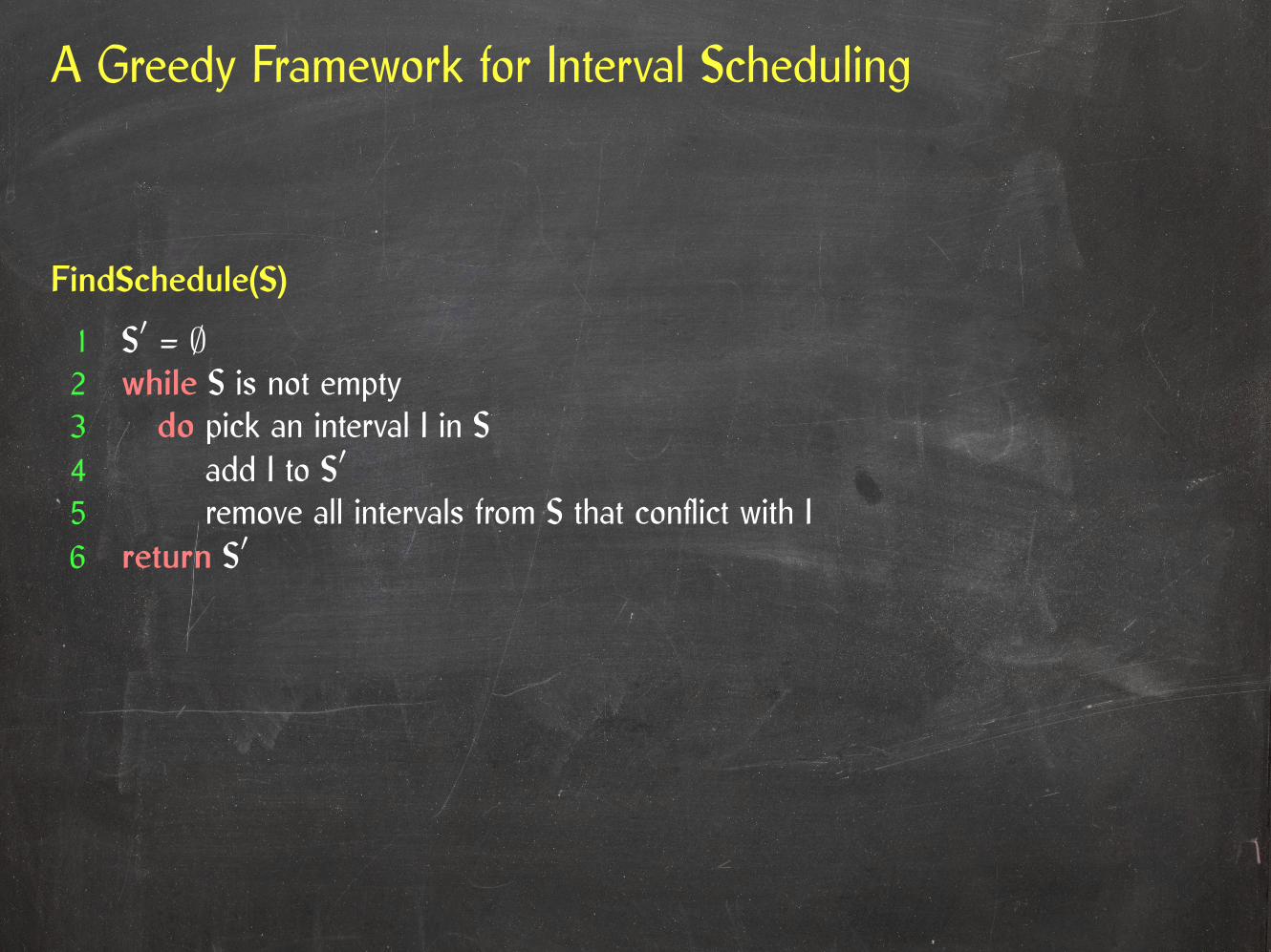
A Greedy Framework for Interval Scheduling
FindSchedule(S)
1 S′ = ∅2 while S is not empty3 do pick an interval I in S4 add I to S′
5 remove all intervals from S that conflict with I6 return S′
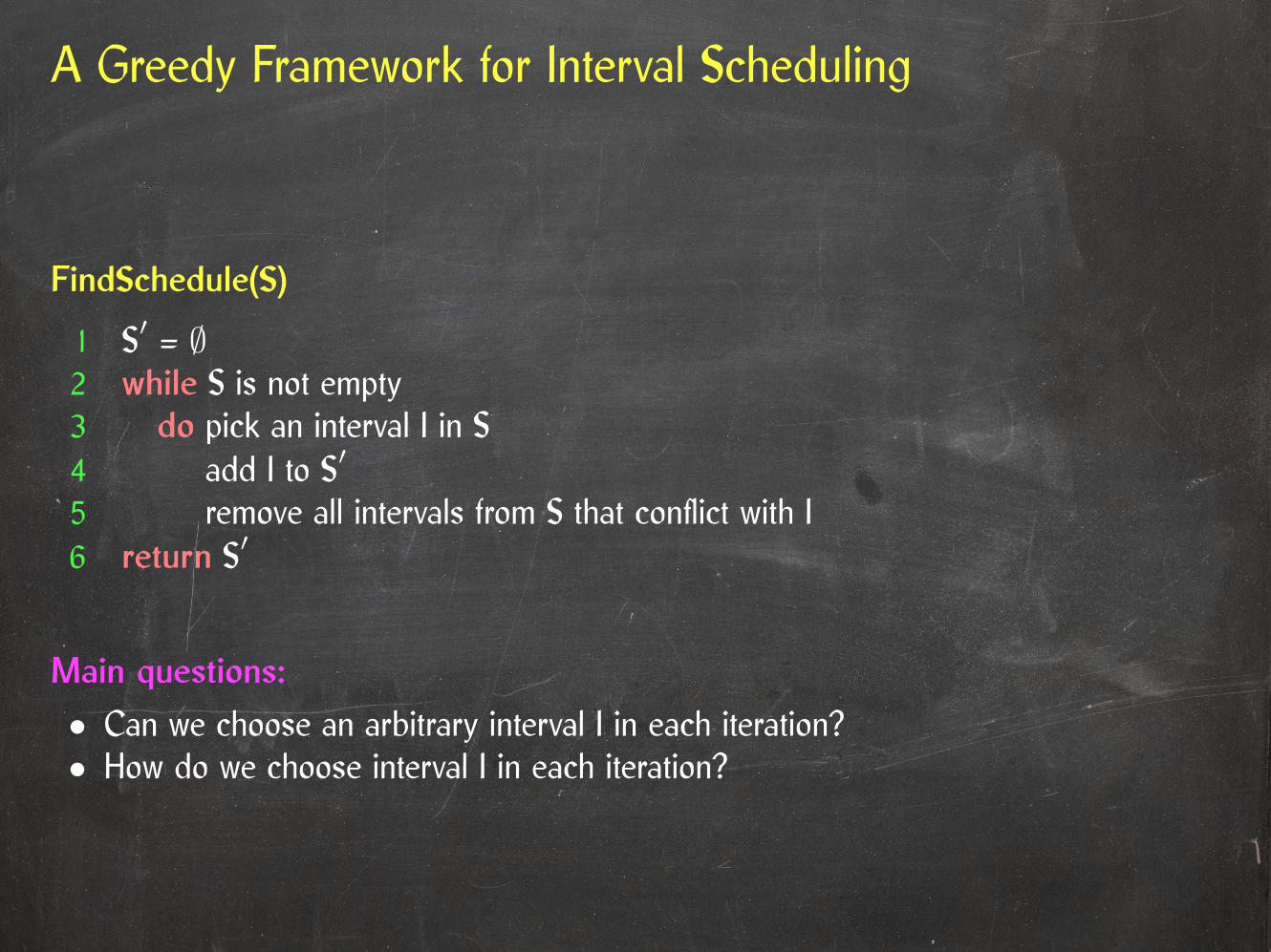
A Greedy Framework for Interval Scheduling
FindSchedule(S)
1 S′ = ∅2 while S is not empty3 do pick an interval I in S4 add I to S′
5 remove all intervals from S that conflict with I6 return S′
Main questions:
• Can we choose an arbitrary interval I in each iteration?• How do we choose interval I in each iteration?

Greedy Strategies for Interval Scheduling

Greedy Strategies for Interval Scheduling
Choose the interval that starts first.

Greedy Strategies for Interval Scheduling
Choose the interval that starts first.

Greedy Strategies for Interval Scheduling
Choose the interval that starts first.
Choose the shortest interval.

Greedy Strategies for Interval Scheduling
Choose the interval that starts first.
Choose the shortest interval.
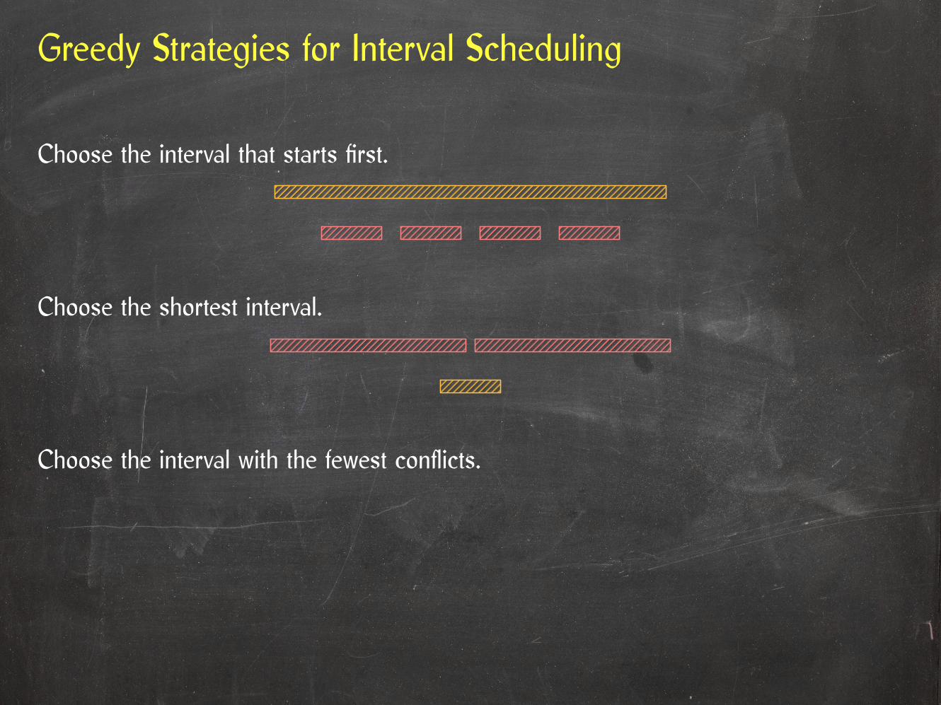
Greedy Strategies for Interval Scheduling
Choose the interval that starts first.
Choose the shortest interval.
Choose the interval with the fewest conflicts.

Greedy Strategies for Interval Scheduling
Choose the interval that starts first.
Choose the shortest interval.
Choose the interval with the fewest conflicts.

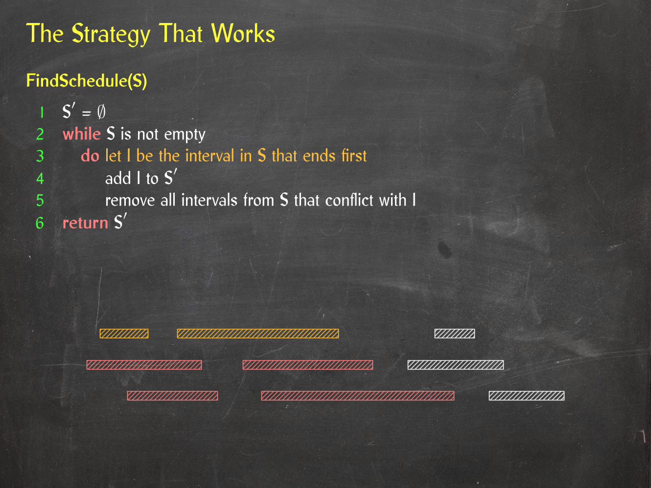
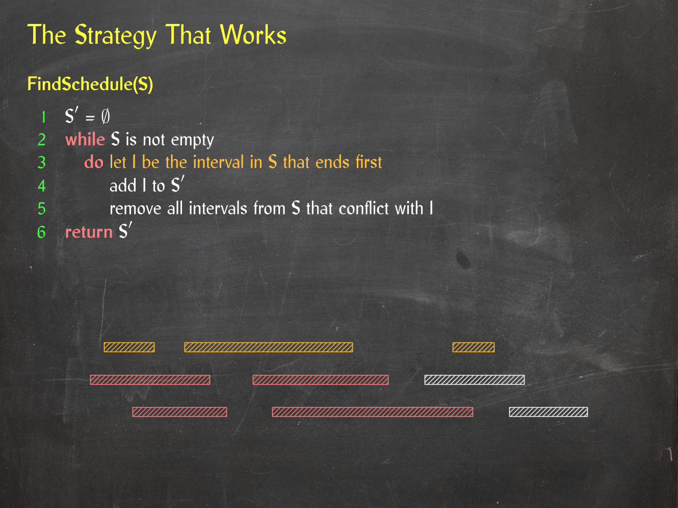
The Strategy That Works
FindSchedule(S)
1 S′ = ∅2 while S is not empty3 do let I be the interval in S that ends first4 add I to S′
5 remove all intervals from S that conflict with I6 return S′

The Strategy That Works
FindSchedule(S)
1 S′ = ∅2 while S is not empty3 do let I be the interval in S that ends first4 add I to S′
5 remove all intervals from S that conflict with I6 return S′

The Strategy That Works
FindSchedule(S)
1 S′ = ∅2 while S is not empty3 do let I be the interval in S that ends first4 add I to S′
5 remove all intervals from S that conflict with I6 return S′

The Strategy That Works
FindSchedule(S)
1 S′ = ∅2 while S is not empty3 do let I be the interval in S that ends first4 add I to S′
5 remove all intervals from S that conflict with I6 return S′
The Strategy That Works
FindSchedule(S)
1 S′ = ∅2 while S is not empty3 do let I be the interval in S that ends first4 add I to S′
5 remove all intervals from S that conflict with I6 return S′
The Strategy That Works
FindSchedule(S)
1 S′ = ∅2 while S is not empty3 do let I be the interval in S that ends first4 add I to S′
5 remove all intervals from S that conflict with I6 return S′

The Strategy That Works
FindSchedule(S)
1 S′ = ∅2 while S is not empty3 do let I be the interval in S that ends first4 add I to S′
5 remove all intervals from S that conflict with I6 return S′

The Strategy That Works
FindSchedule(S)
1 S′ = ∅2 while S is not empty3 do let I be the interval in S that ends first4 add I to S′
5 remove all intervals from S that conflict with I6 return S′

The Greedy Algorithm Stays Ahead
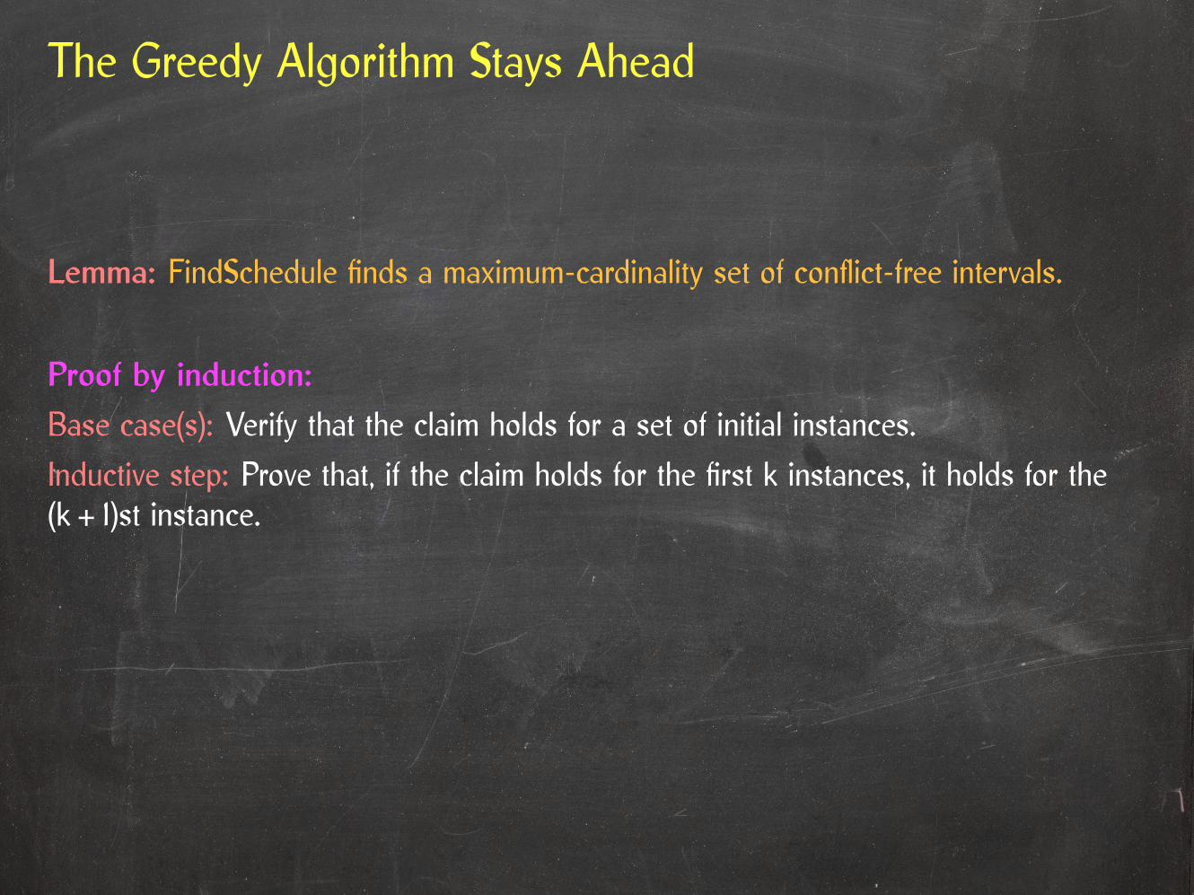
Lemma: FindSchedule finds a maximum-cardinality set of conflict-free intervals.

The Greedy Algorithm Stays Ahead
Lemma: FindSchedule finds a maximum-cardinality set of conflict-free intervals.
Let I1 ≺ I2 ≺ · · · ≺ Ik be the schedule we compute.
Let O1 ≺ O2 ≺ · · · ≺ Om be an optimal schedule.
Prove by induction on j that Ij ends no later than Oj.

The Greedy Algorithm Stays Ahead
Lemma: FindSchedule finds a maximum-cardinality set of conflict-free intervals.
⇒ Since Oj+1 starts after Oj ends, it also starts after Ij ends.
⇒ If k < m, FindSchedule inspects Ok+1 after Ik and thus would have added it to itsoutput, a contradiction.
Let I1 ≺ I2 ≺ · · · ≺ Ik be the schedule we compute.
Let O1 ≺ O2 ≺ · · · ≺ Om be an optimal schedule.
Prove by induction on j that Ij ends no later than Oj.
The Greedy Algorithm Stays Ahead
Proof by induction:
Base case(s): Verify that the claim holds for a set of initial instances.
Inductive step: Prove that, if the claim holds for the first k instances, it holds for the(k + 1)st instance.
Lemma: FindSchedule finds a maximum-cardinality set of conflict-free intervals.

The Greedy Algorithm Stays Ahead
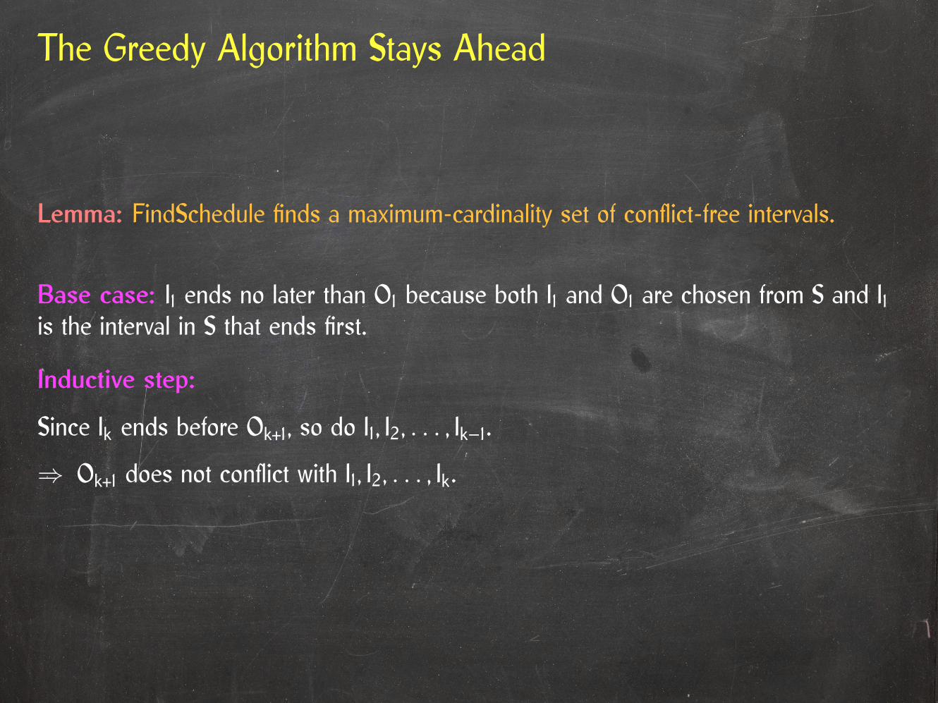
Lemma: FindSchedule finds a maximum-cardinality set of conflict-free intervals.
Base case: I1 ends no later than O1 because both I1 and O1 are chosen from S and I1is the interval in S that ends first.

The Greedy Algorithm Stays Ahead
Lemma: FindSchedule finds a maximum-cardinality set of conflict-free intervals.
Base case: I1 ends no later than O1 because both I1 and O1 are chosen from S and I1is the interval in S that ends first.
Inductive step:
Since Ik ends before Ok+1, so do I1, I2, . . . , Ik–1.
⇒ Ok+1 does not conflict with I1, I2, . . . , Ik.
⇒ Ik+1 ends no later than Ok+1 because it is the interval that ends first among allintervals that do not conflict with I1, I2, . . . , Ik.
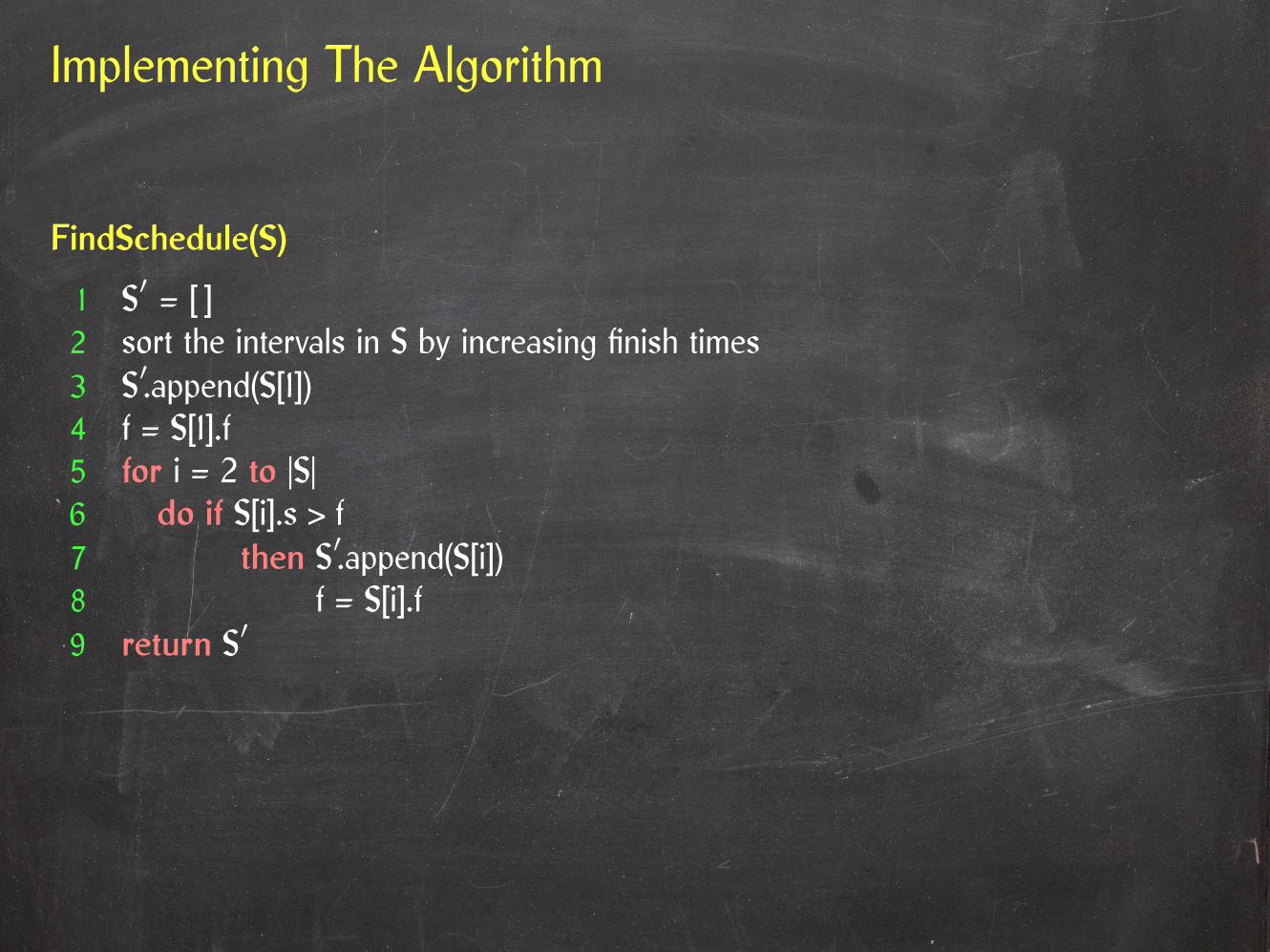
Implementing The Algorithm
FindSchedule(S)
1 S′ = [ ]2 sort the intervals in S by increasing finish times3 S′.append(S[1])4 f = S[1].f5 for i = 2 to |S|6 do if S[i].s > f7 then S′.append(S[i])8 f = S[i].f9 return S′

Implementing The Algorithm
FindSchedule(S)
1 S′ = [ ]2 sort the intervals in S by increasing finish times3 S′.append(S[1])4 f = S[1].f5 for i = 2 to |S|6 do if S[i].s > f7 then S′.append(S[i])8 f = S[i].f9 return S′
Lemma: A maximum-cardinality set of non-conflicting intervals can be found inO(n lg n) time.

Minimum Spanning Tree
⇒ We want the cheapest possible network.
Given: n computers
Goal: Connect them so that every computer can communicate with every othercomputer.
We don’t care whether theconnection between any pairof computers is short.
We don’t care about faulttolerance.
Every foot of cable costs us $1.

Minimum Spanning Tree
Given a graph G = (V, E) and an assignment of weights (costs) to the edges of G, aminimum spanning tree (MST) T of G is a spanning tree with minimum total weight
w(T) =∑e∈T
w(e).
6
1
3
5
4
7
8
3
1
2
97
6
3
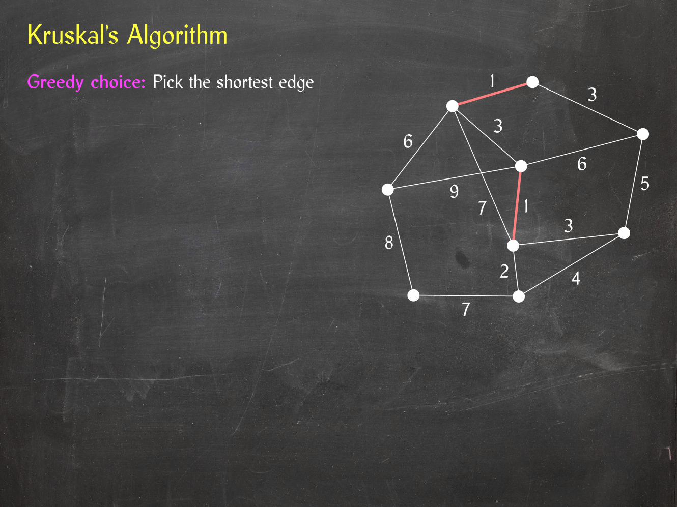
Kruskal’s Algorithm
Greedy choice: Pick the shortest edge
6
1
3
5
4
7
8
3
1
2
97
6
3

Kruskal’s Algorithm
6
1
3
5
4
7
8
3
1
2
97
6
3
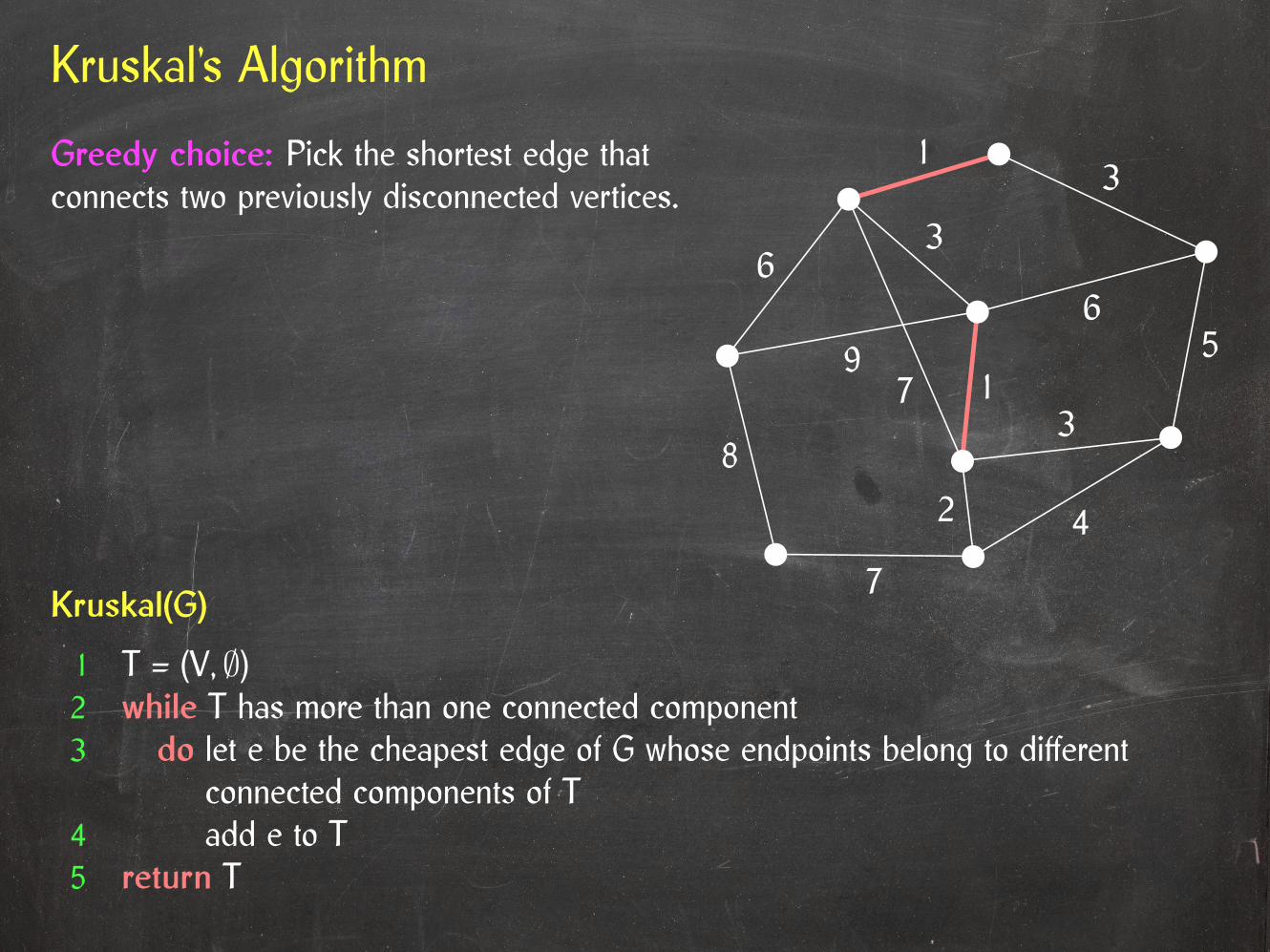
Greedy choice: Pick the shortest edge thatconnects two previously disconnected vertices.
Kruskal’s Algorithm
Kruskal(G)
1 T = (V, ∅)2 while T has more than one connected component3 do let e be the cheapest edge of G whose endpoints belong to di�erent
connected components of T4 add e to T5 return T
6
1
3
5
4
7
8
3
1
2
97
6
3
Greedy choice: Pick the shortest edge thatconnects two previously disconnected vertices.

A Cut Theorem
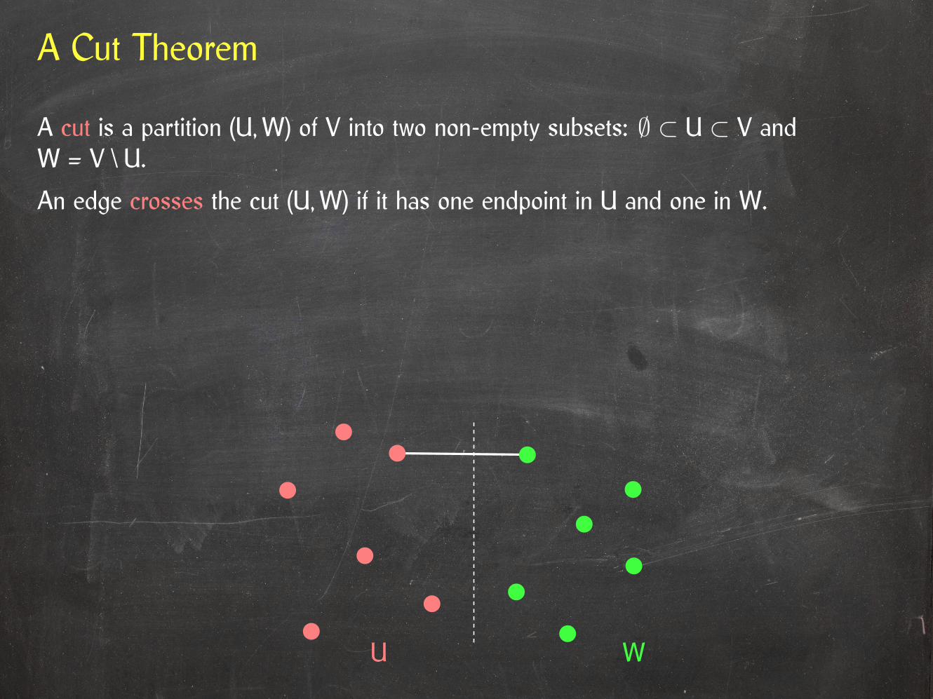
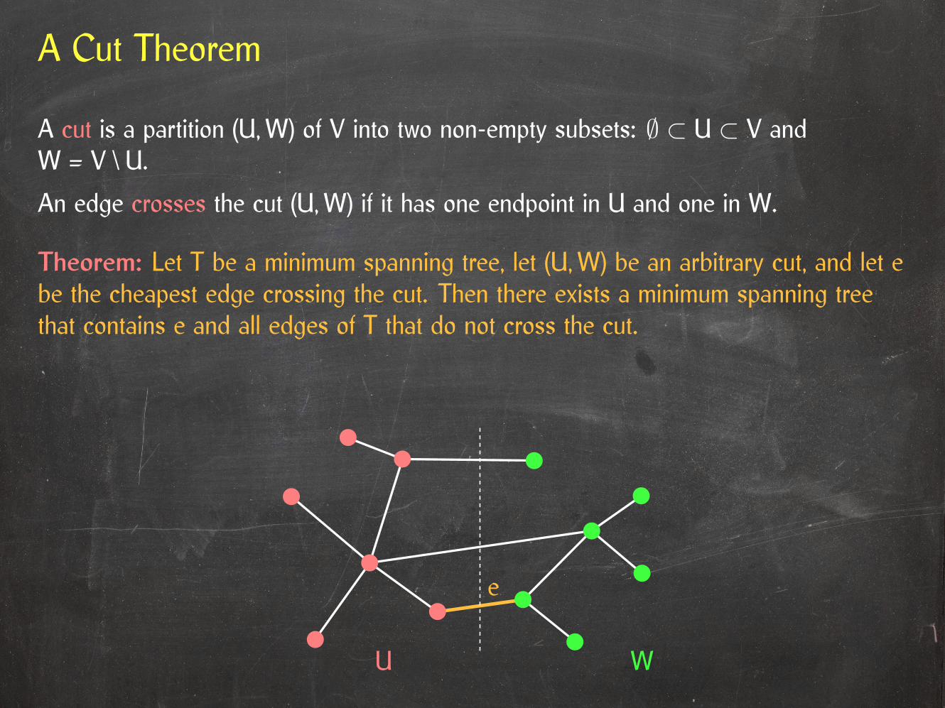
A cut is a partition (U,W) of V into two non-empty subsets: ∅ ⊂ U ⊂ V andW = V \ U.
U W
A Cut Theorem
A cut is a partition (U,W) of V into two non-empty subsets: ∅ ⊂ U ⊂ V andW = V \ U.
An edge crosses the cut (U,W) if it has one endpoint in U and one in W.
U W
A Cut Theorem
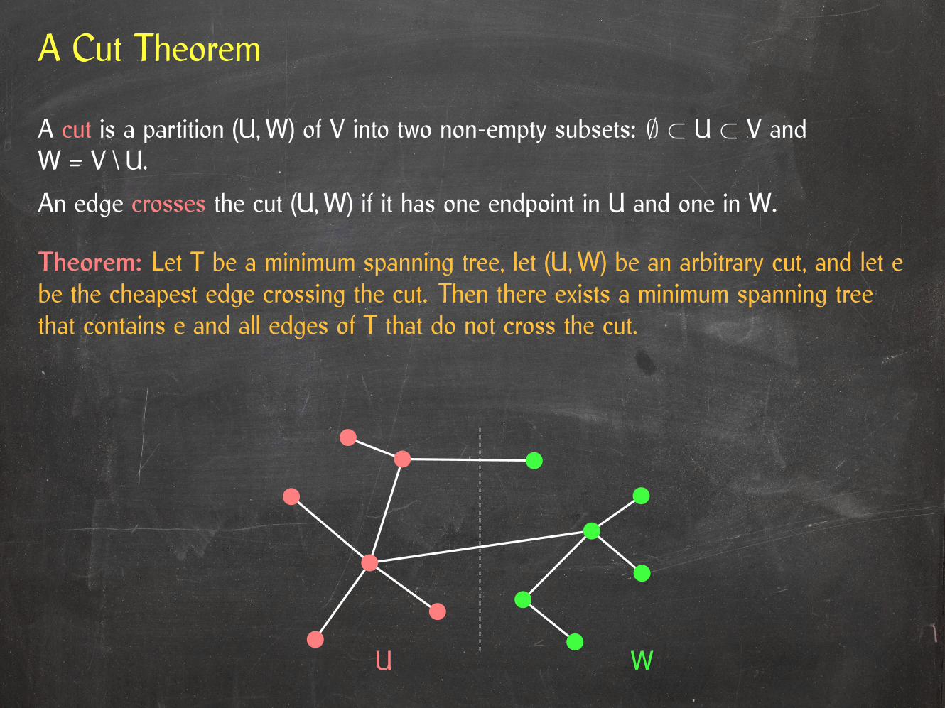
Theorem: Let T be a minimum spanning tree, let (U,W) be an arbitrary cut, and let ebe the cheapest edge crossing the cut. Then there exists a minimum spanning treethat contains e and all edges of T that do not cross the cut.
A cut is a partition (U,W) of V into two non-empty subsets: ∅ ⊂ U ⊂ V andW = V \ U.
An edge crosses the cut (U,W) if it has one endpoint in U and one in W.
U W
A Cut Theorem
Theorem: Let T be a minimum spanning tree, let (U,W) be an arbitrary cut, and let ebe the cheapest edge crossing the cut. Then there exists a minimum spanning treethat contains e and all edges of T that do not cross the cut.
A cut is a partition (U,W) of V into two non-empty subsets: ∅ ⊂ U ⊂ V andW = V \ U.
An edge crosses the cut (U,W) if it has one endpoint in U and one in W.
U W
e

A Cut Theorem
Theorem: Let T be a minimum spanning tree, let (U,W) be an arbitrary cut, and let ebe the cheapest edge crossing the cut. Then there exists a minimum spanning treethat contains e and all edges of T that do not cross the cut.
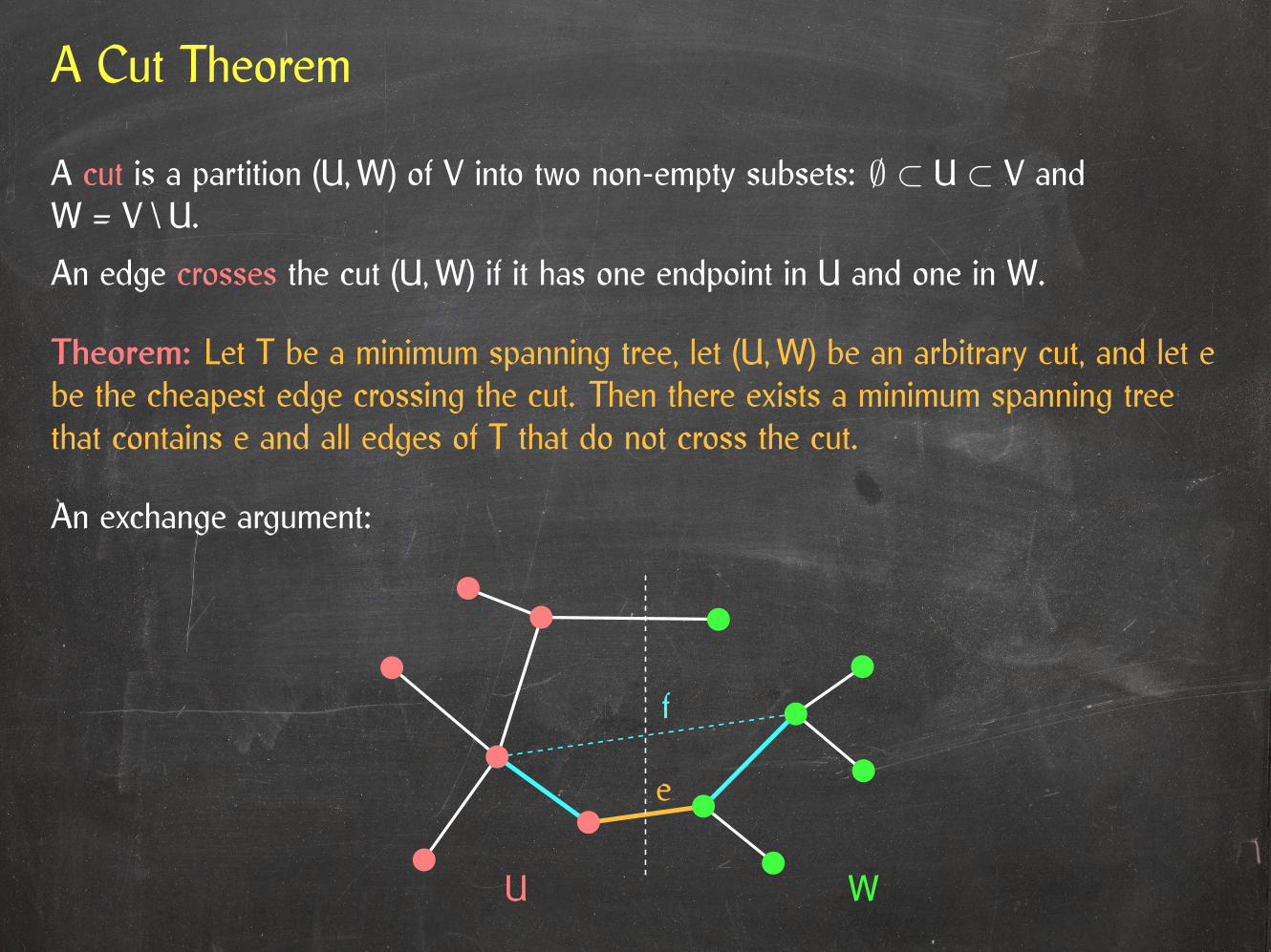
An exchange argument:
A cut is a partition (U,W) of V into two non-empty subsets: ∅ ⊂ U ⊂ V andW = V \ U.
An edge crosses the cut (U,W) if it has one endpoint in U and one in W.
U W
e

A Cut Theorem
Theorem: Let T be a minimum spanning tree, let (U,W) be an arbitrary cut, and let ebe the cheapest edge crossing the cut. Then there exists a minimum spanning treethat contains e and all edges of T that do not cross the cut.
An exchange argument:
A cut is a partition (U,W) of V into two non-empty subsets: ∅ ⊂ U ⊂ V andW = V \ U.
An edge crosses the cut (U,W) if it has one endpoint in U and one in W.
U W
e
f

Correctness Of Kruskal’s Algorithm
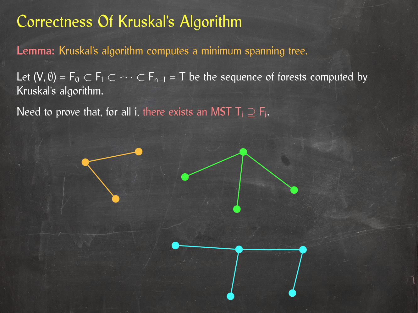
Lemma: Kruskal’s algorithm computes a minimum spanning tree.

Correctness Of Kruskal’s Algorithm
Lemma: Kruskal’s algorithm computes a minimum spanning tree.
Let (V, ∅) = F0 ⊂ F1 ⊂ · · · ⊂ Fn–1 = T be the sequence of forests computed byKruskal’s algorithm.

Correctness Of Kruskal’s Algorithm
Lemma: Kruskal’s algorithm computes a minimum spanning tree.
Let (V, ∅) = F0 ⊂ F1 ⊂ · · · ⊂ Fn–1 = T be the sequence of forests computed byKruskal’s algorithm.
Need to prove that, for all i, there exists an MST Ti ⊇ Fi.
Correctness Of Kruskal’s Algorithm
Lemma: Kruskal’s algorithm computes a minimum spanning tree.
Let (V, ∅) = F0 ⊂ F1 ⊂ · · · ⊂ Fn–1 = T be the sequence of forests computed byKruskal’s algorithm.
Need to prove that, for all i, there exists an MST Ti ⊇ Fi.

Correctness Of Kruskal’s Algorithm
Lemma: Kruskal’s algorithm computes a minimum spanning tree.
Let (V, ∅) = F0 ⊂ F1 ⊂ · · · ⊂ Fn–1 = T be the sequence of forests computed byKruskal’s algorithm.
Need to prove that, for all i, there exists an MST Ti ⊇ Fi.
e

Correctness Of Kruskal’s Algorithm
Lemma: Kruskal’s algorithm computes a minimum spanning tree.
Let (V, ∅) = F0 ⊂ F1 ⊂ · · · ⊂ Fn–1 = T be the sequence of forests computed byKruskal’s algorithm.
Need to prove that, for all i, there exists an MST Ti ⊇ Fi.
e
Implementing Kruskal’s Algorithm
Kruskal(G)
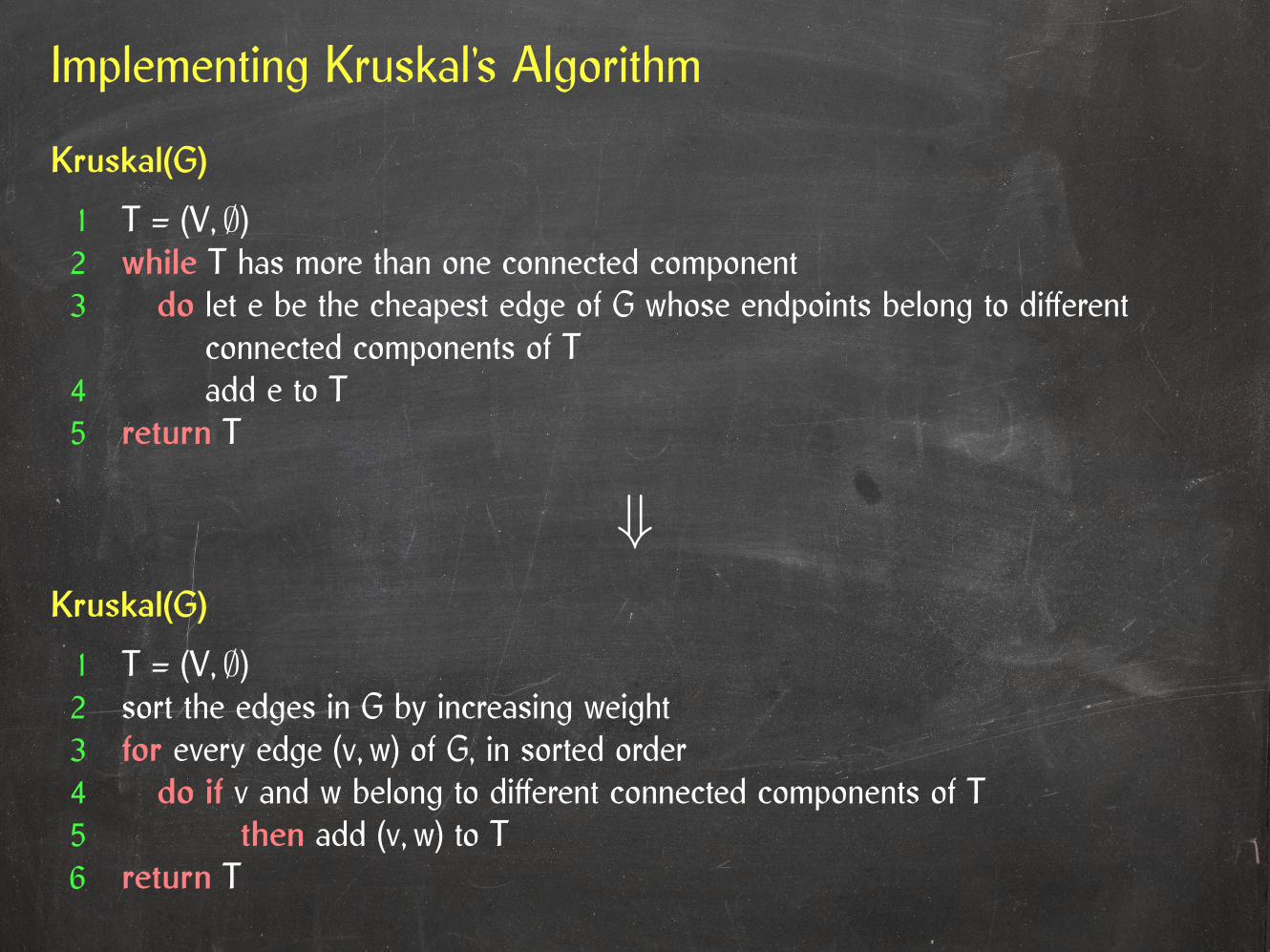
1 T = (V, ∅)2 sort the edges in G by increasing weight3 for every edge (v, w) of G, in sorted order4 do if v and w belong to di�erent connected components of T5 then add (v, w) to T6 return T
Kruskal(G)
1 T = (V, ∅)2 while T has more than one connected component3 do let e be the cheapest edge of G whose endpoints belong to di�erent
connected components of T4 add e to T5 return T
⇓

A Union-Find Data Structure
2
8
6
5
7
10
Given a set S of elements, maintain apartition of S into subsets S1, S2, . . . , Sk.
13
9
4
A Union-Find Data Structure
2
8
6
5
7
10
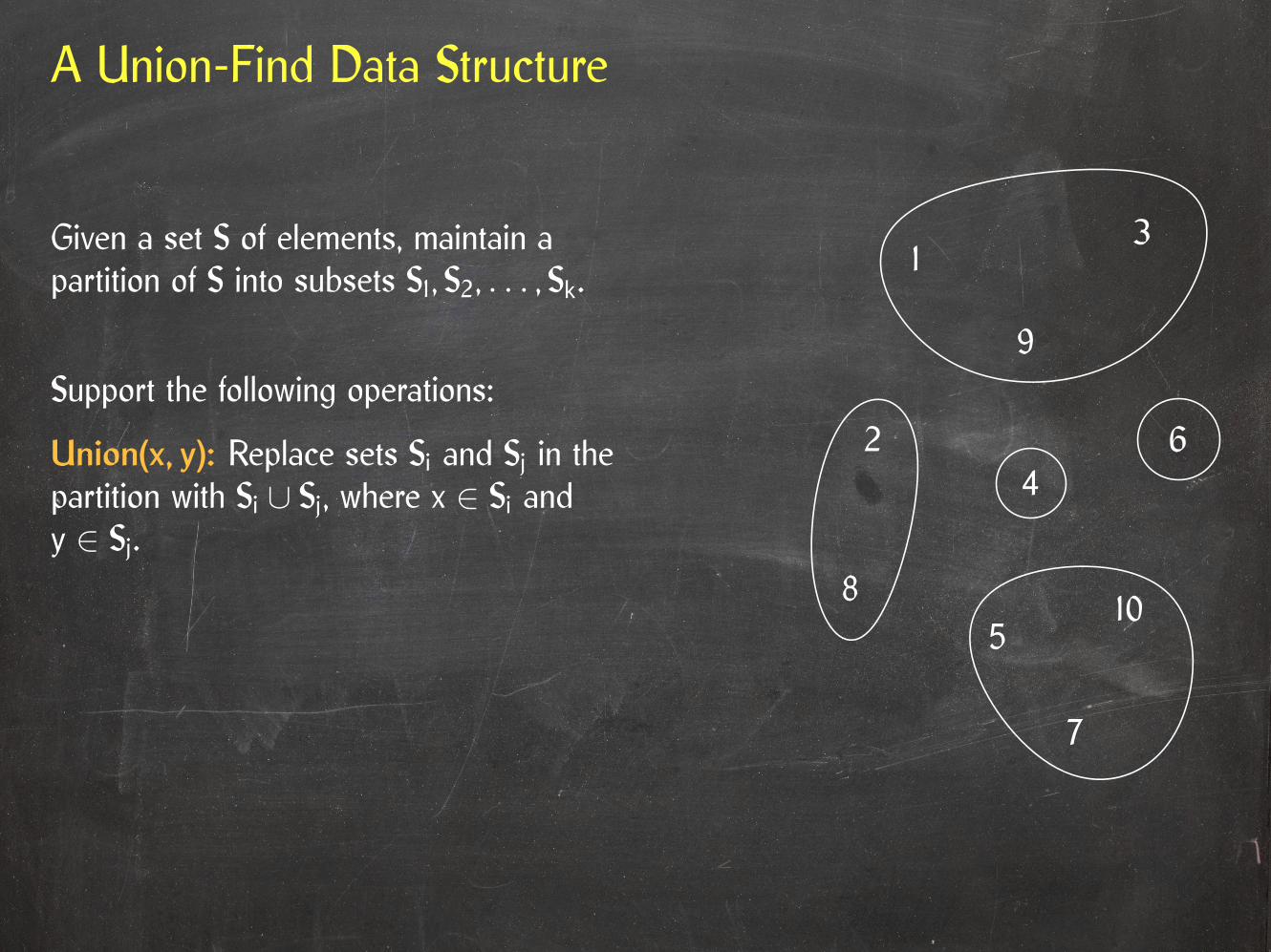
Given a set S of elements, maintain apartition of S into subsets S1, S2, . . . , Sk.
Support the following operations:
Union(x, y): Replace sets Si and Sj in thepartition with Si ∪ Sj, where x ∈ Si andy ∈ Sj.
13
9
4

A Union-Find Data Structure
13
2
8
6
5
7
10
Given a set S of elements, maintain apartition of S into subsets S1, S2, . . . , Sk.
Support the following operations:
Union(x, y): Replace sets Si and Sj in thepartition with Si ∪ Sj, where x ∈ Si andy ∈ Sj.
9
4
A Union-Find Data Structure
85
7
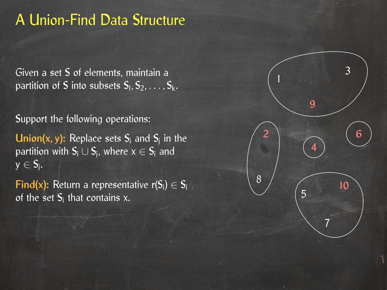
Given a set S of elements, maintain apartition of S into subsets S1, S2, . . . , Sk.
Support the following operations:
Union(x, y): Replace sets Si and Sj in thepartition with Si ∪ Sj, where x ∈ Si andy ∈ Sj.
Find(x): Return a representative r(Si) ∈ Siof the set Si that contains x.
13
2 6
10
9
4
A Union-Find Data Structure
13
85
7
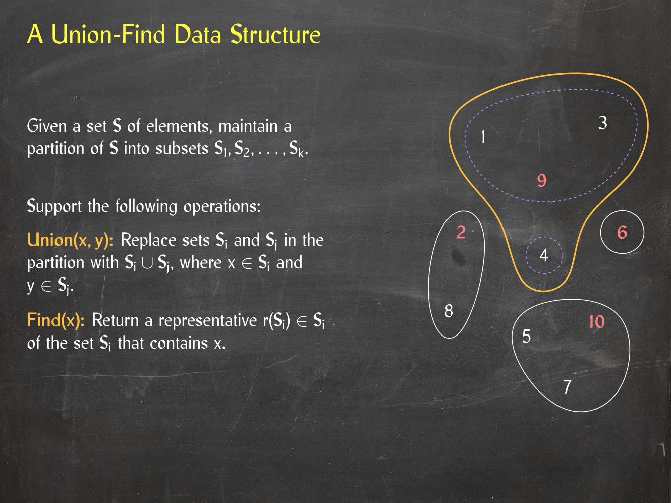
Given a set S of elements, maintain apartition of S into subsets S1, S2, . . . , Sk.
Support the following operations:
Union(x, y): Replace sets Si and Sj in thepartition with Si ∪ Sj, where x ∈ Si andy ∈ Sj.
Find(x): Return a representative r(Si) ∈ Siof the set Si that contains x.
2 6
10
9
4
A Union-Find Data Structure
13
85
7
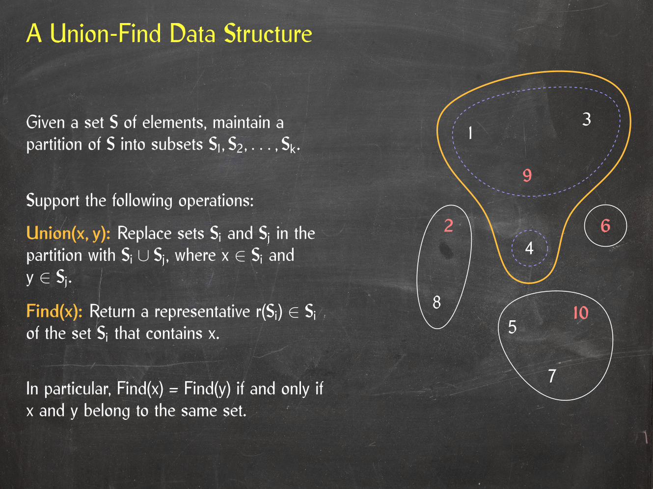
Given a set S of elements, maintain apartition of S into subsets S1, S2, . . . , Sk.
In particular, Find(x) = Find(y) if and only ifx and y belong to the same set.
Support the following operations:
Union(x, y): Replace sets Si and Sj in thepartition with Si ∪ Sj, where x ∈ Si andy ∈ Sj.
Find(x): Return a representative r(Si) ∈ Siof the set Si that contains x.
2 6
10
9
4

Kruskal’s Algorithm Using Union-Find
Kruskal(G)
1 T = (V, ∅)2 initialize a union-find structure D for V with every vertex v ∈ V in its own set3 sort the edges in G by increasing weight4 for every edge (v, w) of G, in sorted order5 do if D.find(v) 6= D.find(w)6 then add (v, w) to T7 D.union(v, w)8 return T
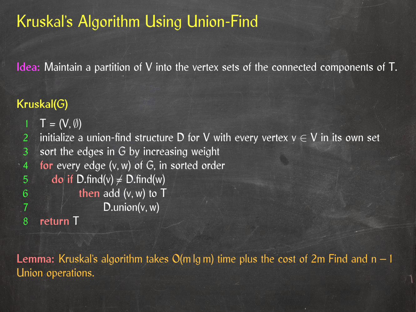
Idea: Maintain a partition of V into the vertex sets of the connected components of T.
Kruskal’s Algorithm Using Union-Find
Kruskal(G)
1 T = (V, ∅)2 initialize a union-find structure D for V with every vertex v ∈ V in its own set3 sort the edges in G by increasing weight4 for every edge (v, w) of G, in sorted order5 do if D.find(v) 6= D.find(w)6 then add (v, w) to T7 D.union(v, w)8 return T
Lemma: Kruskal’s algorithm takes O(m lgm) time plus the cost of 2m Find and n – 1Union operations.
Idea: Maintain a partition of V into the vertex sets of the connected components of T.

A Simple Union-Find Structure
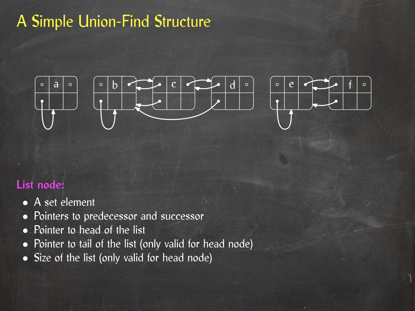
List node:
• A set element• Pointers to predecessor and successor• Pointer to head of the list• Pointer to tail of the list (only valid for head node)• Size of the list (only valid for head node)
a b c d e f
A Simple Union-Find Structure
List node:
• A set element• Pointers to predecessor and successor• Pointer to head of the list• Pointer to tail of the list (only valid for head node)• Size of the list (only valid for head node)
a b c d e f

A Simple Union-Find Structure
List node:
• A set element• Pointers to predecessor and successor• Pointer to head of the list• Pointer to tail of the list (only valid for head node)• Size of the list (only valid for head node)
a b c d e f? ? ?

A Simple Union-Find Structure
List node:
• A set element• Pointers to predecessor and successor• Pointer to head of the list• Pointer to tail of the list (only valid for head node)• Size of the list (only valid for head node)
3
a b c d e f? ? ? ? ? ?21

Find
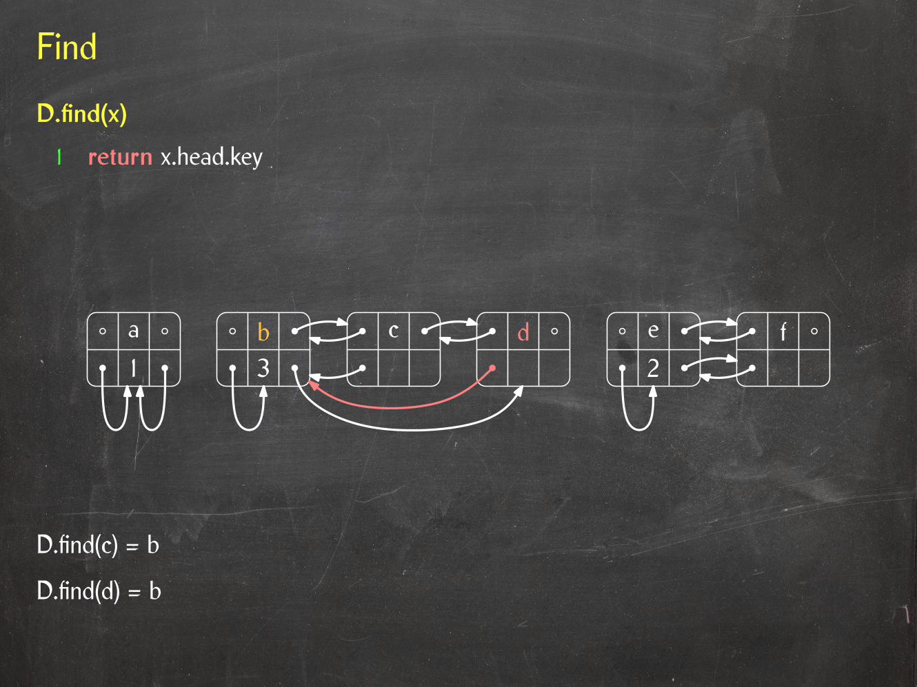
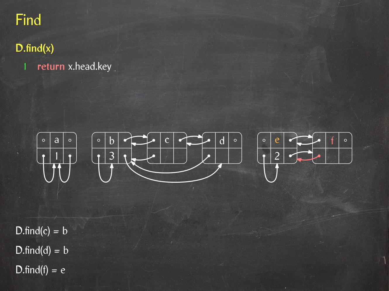
D.find(x)
1 return x.head.key
3
a b c d e f21

Find
D.find(x)
1 return x.head.key
3
a d e f21
D.find(c) = b
b c
Find
D.find(x)
1 return x.head.key
3
a c e f21
D.find(c) = b
D.find(d) = b
b d
Find
D.find(x)
1 return x.head.key
3
a b c d21
D.find(c) = b
D.find(d) = b
D.find(f) = e
e f
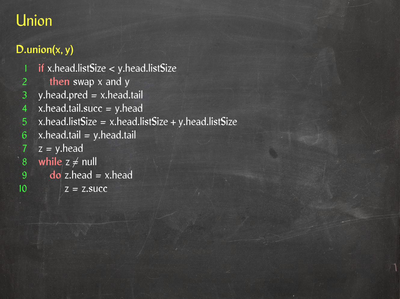
Union
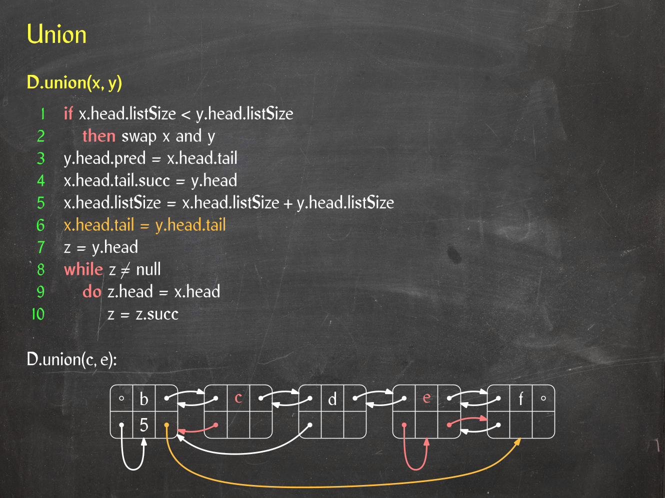
D.union(x, y)
1 if x.head.listSize < y.head.listSize2 then swap x and y3 y.head.pred = x.head.tail4 x.head.tail.succ = y.head5 x.head.listSize = x.head.listSize + y.head.listSize6 x.head.tail = y.head.tail7 z = y.head8 while z 6= null9 do z.head = x.head10 z = z.succ
Union
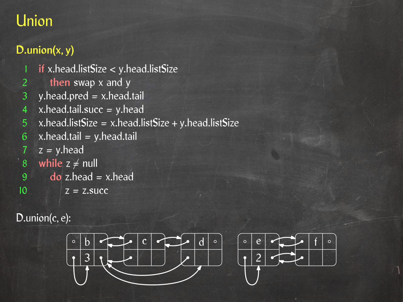
D.union(x, y)
1 if x.head.listSize < y.head.listSize2 then swap x and y3 y.head.pred = x.head.tail4 x.head.tail.succ = y.head5 x.head.listSize = x.head.listSize + y.head.listSize6 x.head.tail = y.head.tail7 z = y.head8 while z 6= null9 do z.head = x.head10 z = z.succ
D.union(c, e):
3b c d e f
2

Union
D.union(c, e):
D.union(x, y)
1 if x.head.listSize < y.head.listSize2 then swap x and y3 y.head.pred = x.head.tail4 x.head.tail.succ = y.head5 x.head.listSize = x.head.listSize + y.head.listSize6 x.head.tail = y.head.tail7 z = y.head8 while z 6= null9 do z.head = x.head10 z = z.succ
3b c d e f
2

Union
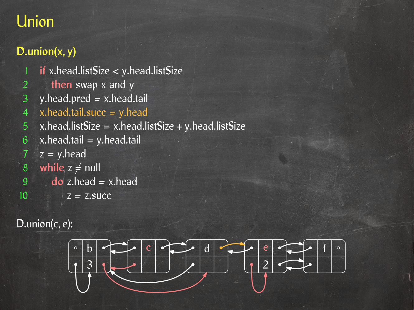
D.union(c, e):
D.union(x, y)
1 if x.head.listSize < y.head.listSize2 then swap x and y3 y.head.pred = x.head.tail4 x.head.tail.succ = y.head5 x.head.listSize = x.head.listSize + y.head.listSize6 x.head.tail = y.head.tail7 z = y.head8 while z 6= null9 do z.head = x.head10 z = z.succ
3b c d e f
2
Union
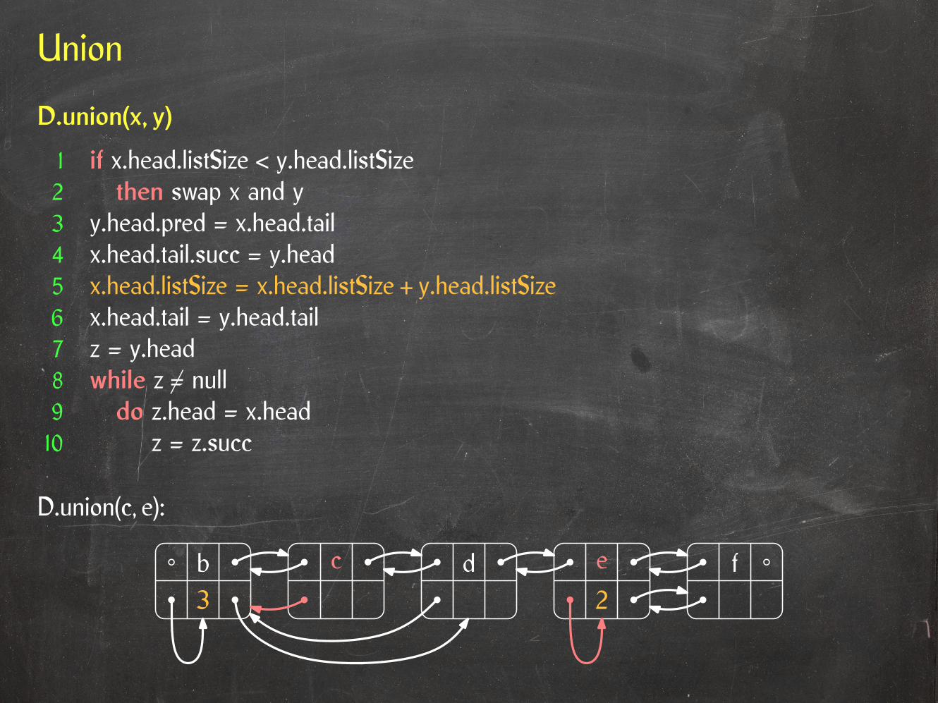
D.union(c, e):
D.union(x, y)
1 if x.head.listSize < y.head.listSize2 then swap x and y3 y.head.pred = x.head.tail4 x.head.tail.succ = y.head5 x.head.listSize = x.head.listSize + y.head.listSize6 x.head.tail = y.head.tail7 z = y.head8 while z 6= null9 do z.head = x.head10 z = z.succ
3b c d e f
2
Union
D.union(c, e):
D.union(x, y)
1 if x.head.listSize < y.head.listSize2 then swap x and y3 y.head.pred = x.head.tail4 x.head.tail.succ = y.head5 x.head.listSize = x.head.listSize + y.head.listSize6 x.head.tail = y.head.tail7 z = y.head8 while z 6= null9 do z.head = x.head10 z = z.succ
3b c d e f
2

Union
D.union(c, e):
D.union(x, y)
1 if x.head.listSize < y.head.listSize2 then swap x and y3 y.head.pred = x.head.tail4 x.head.tail.succ = y.head5 x.head.listSize = x.head.listSize + y.head.listSize6 x.head.tail = y.head.tail7 z = y.head8 while z 6= null9 do z.head = x.head10 z = z.succ
5b c d e f
?
Union
D.union(c, e):
D.union(x, y)
1 if x.head.listSize < y.head.listSize2 then swap x and y3 y.head.pred = x.head.tail4 x.head.tail.succ = y.head5 x.head.listSize = x.head.listSize + y.head.listSize6 x.head.tail = y.head.tail7 z = y.head8 while z 6= null9 do z.head = x.head10 z = z.succ
5b c d e f

Union
D.union(c, e):
D.union(x, y)
1 if x.head.listSize < y.head.listSize2 then swap x and y3 y.head.pred = x.head.tail4 x.head.tail.succ = y.head5 x.head.listSize = x.head.listSize + y.head.listSize6 x.head.tail = y.head.tail7 z = y.head8 while z 6= null9 do z.head = x.head10 z = z.succ
5b c d e f
?

Union
D.union(c, e):
D.union(x, y)
1 if x.head.listSize < y.head.listSize2 then swap x and y3 y.head.pred = x.head.tail4 x.head.tail.succ = y.head5 x.head.listSize = x.head.listSize + y.head.listSize6 x.head.tail = y.head.tail7 z = y.head8 while z 6= null9 do z.head = x.head10 z = z.succ
5b c d e f

Union
D.union(c, e):
D.union(x, y)
1 if x.head.listSize < y.head.listSize2 then swap x and y3 y.head.pred = x.head.tail4 x.head.tail.succ = y.head5 x.head.listSize = x.head.listSize + y.head.listSize6 x.head.tail = y.head.tail7 z = y.head8 while z 6= null9 do z.head = x.head10 z = z.succ
5b c d e f

Analysis
Observation: A Find operation takes constant time.
Analysis
Observation: A Find operation takes constant time.
Observation: A Union operation takes O(1 + s) time, where s is the size of the smallerlist.

Analysis
Observation: A Find operation takes constant time.
Observation: A Union operation takes O(1 + s) time, where s is the size of the smallerlist.
Corollary: The total cost of m operations over a base set S is O(m +
∑x∈S c(x)
),
where c(x) is the number of times x is in the smaller list of a Union operation.
Lemma: Let s(x, i) be the size of the list containing x after x was in the smaller list of iUnion operations. Then s(x, i) ≥ 2i.
Base case: i = 0. The list containing x has size at least 1 = 20.
Inductive step: i > 0.
• Consider the ith Union operation where x is in the smaller list.• Let S1 and S2 be the two unioned lists and assume x ∈ S2.• Then |S1| ≥ |S2| ≥ 2i–1.• Thus, |S1 ∪ S2| ≥ 2i.

Analysis
Observation: A Find operation takes constant time.
Observation: A Union operation takes O(1 + s) time, where s is the size of the smallerlist.
Corollary: The total cost of m operations over a base set S is O(m +
∑x∈S c(x)
),
where c(x) is the number of times x is in the smaller list of a Union operation.
Lemma: Let s(x, i) be the size of the list containing x after x was in the smaller list of iUnion operations. Then s(x, i) ≥ 2i.
Corollary: c(x) ≤ lg n for all x ∈ S.
Base case: i = 0. The list containing x has size at least 1 = 20.
Inductive step: i > 0.
• Consider the ith Union operation where x is in the smaller list.• Let S1 and S2 be the two unioned lists and assume x ∈ S2.• Then |S1| ≥ |S2| ≥ 2i–1.• Thus, |S1 ∪ S2| ≥ 2i.
Analysis
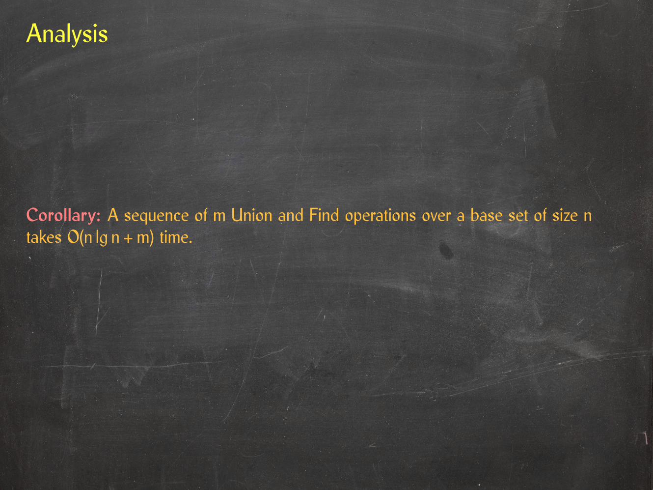
Corollary: A sequence of m Union and Find operations over a base set of size ntakes O(n lg n + m) time.

Analysis
Corollary: A sequence of m Union and Find operations over a base set of size ntakes O(n lg n + m) time.
Corollary: Kruskal’s algorithm takes O(n lg n + m lgm) time.
Analysis
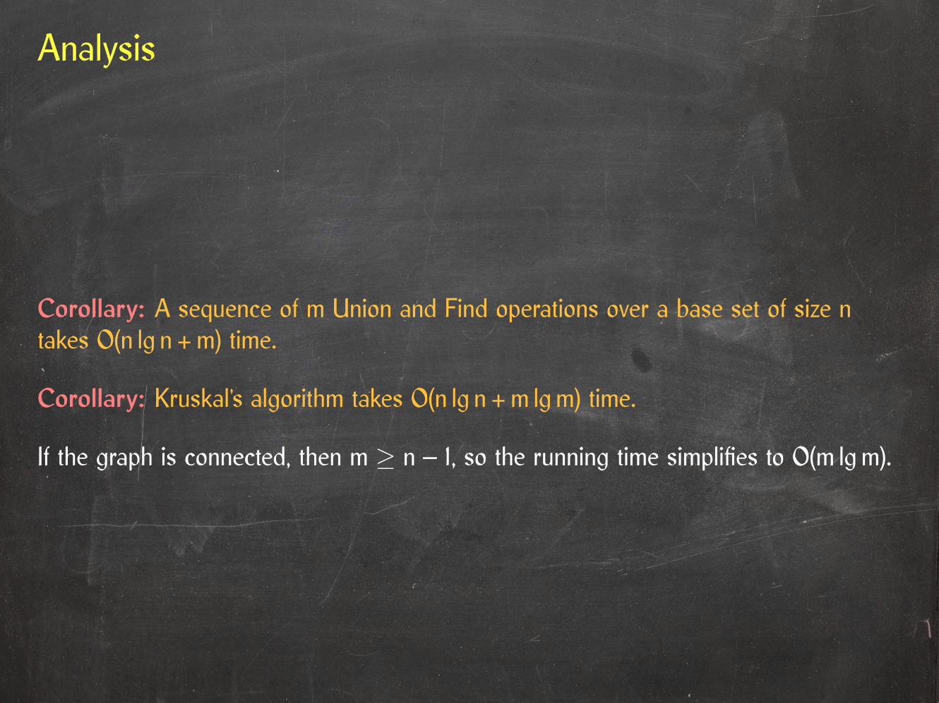
Corollary: A sequence of m Union and Find operations over a base set of size ntakes O(n lg n + m) time.
Corollary: Kruskal’s algorithm takes O(n lg n + m lgm) time.
If the graph is connected, then m ≥ n – 1, so the running time simplifies to O(m lgm).

The Cut Theorem And Graph Traversal
Explored
“Explorable”
Unexplored
Source

The Cut Theorem And Graph Traversal
If there exists an MST containing all green edges, then there exists an MST containingall green edges and the cheapest red edge.
Explored
“Explorable”
Unexplored
Source

The Cut Theorem And Graph Traversal
If there exists an MST containing all green edges, then there exists an MST containingall green edges and the cheapest red edge.
Cut: U = explored vertices, W = V \ U
Explored
“Explorable”
Unexplored
Source
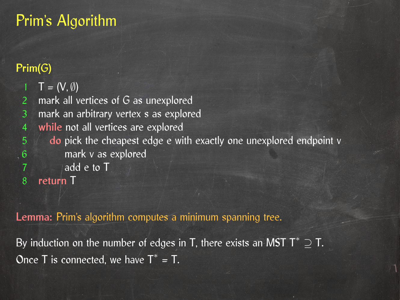
Prim’s Algorithm
Prim(G)
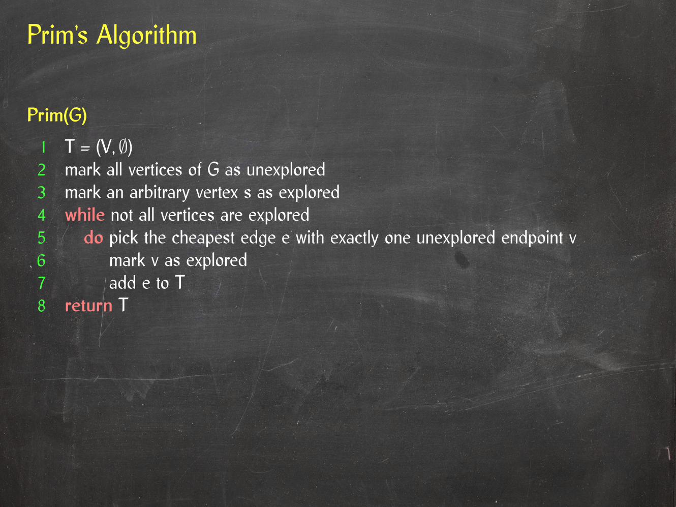
1 T = (V, ∅)2 mark all vertices of G as unexplored3 mark an arbitrary vertex s as explored4 while not all vertices are explored5 do pick the cheapest edge e with exactly one unexplored endpoint v6 mark v as explored7 add e to T8 return T
Prim’s Algorithm
Prim(G)
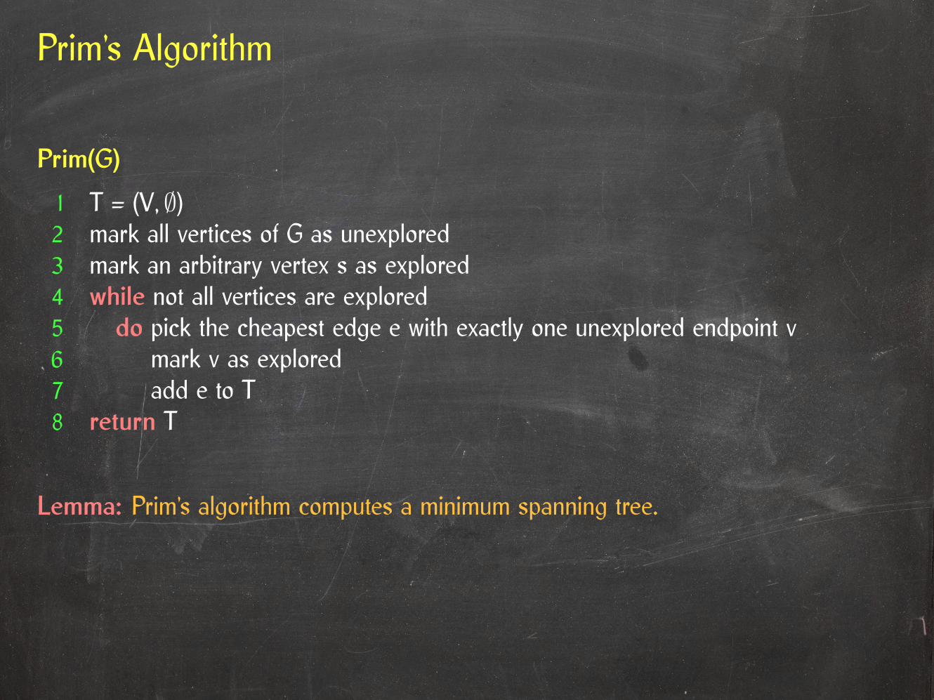
1 T = (V, ∅)2 mark all vertices of G as unexplored3 mark an arbitrary vertex s as explored4 while not all vertices are explored5 do pick the cheapest edge e with exactly one unexplored endpoint v6 mark v as explored7 add e to T8 return T
Lemma: Prim’s algorithm computes a minimum spanning tree.

Prim’s Algorithm
Prim(G)
1 T = (V, ∅)2 mark all vertices of G as unexplored3 mark an arbitrary vertex s as explored4 while not all vertices are explored5 do pick the cheapest edge e with exactly one unexplored endpoint v6 mark v as explored7 add e to T8 return T
Lemma: Prim’s algorithm computes a minimum spanning tree.
By induction on the number of edges in T, there exists an MST T∗ ⊇ T.
Once T is connected, we have T∗ = T.
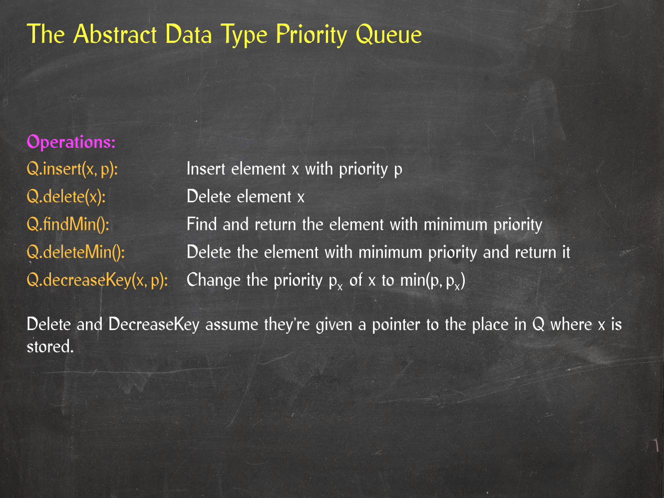
The Abstract Data Type Priority Queue
Operations:Q.insert(x, p): Insert element x with priority p
Q.delete(x): Delete element x
Q.findMin(): Find and return the element with minimum priority
Q.deleteMin(): Delete the element with minimum priority and return it
Q.decreaseKey(x, p): Change the priority px of x to min(p, px)
Delete and DecreaseKey assume they’re given a pointer to the place in Q where x isstored.

The Abstract Data Type Priority Queue
Example: A binary heap is a priority queue supporting all operations in O(lg |Q|) time.
Operations:Q.insert(x, p): Insert element x with priority p
Q.delete(x): Delete element x
Q.findMin(): Find and return the element with minimum priority
Q.deleteMin(): Delete the element with minimum priority and return it
Q.decreaseKey(x, p): Change the priority px of x to min(p, px)
Delete and DecreaseKey assume they’re given a pointer to the place in Q where x isstored.
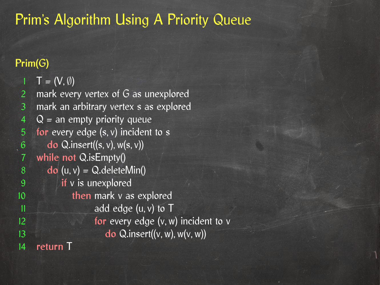
Prim’s Algorithm Using A Priority Queue
Prim(G)
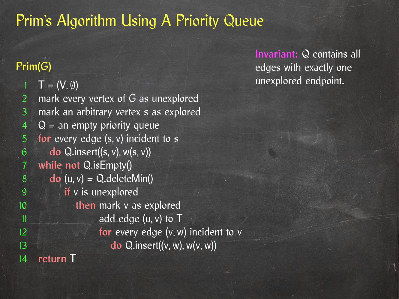
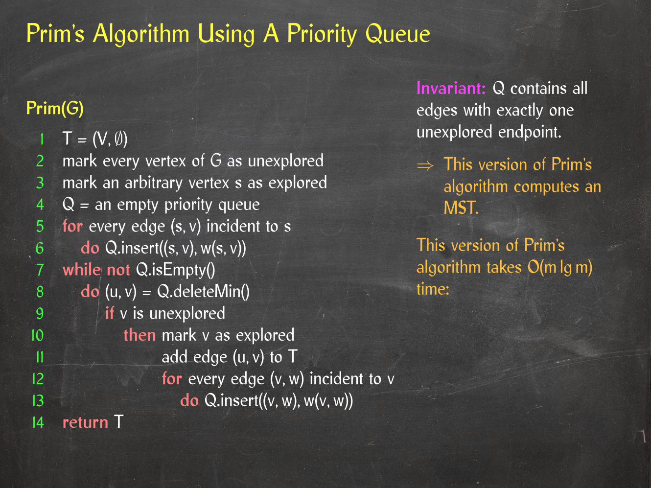
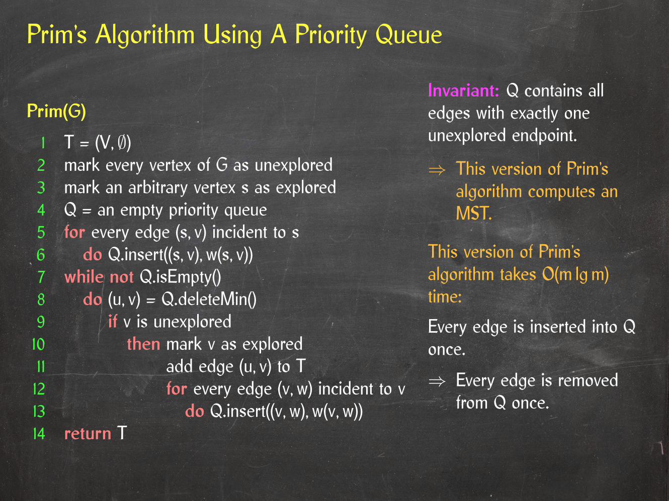
1 T = (V, ∅)2 mark every vertex of G as unexplored3 mark an arbitrary vertex s as explored4 Q = an empty priority queue5 for every edge (s, v) incident to s6 do Q.insert((s, v), w(s, v))7 while not Q.isEmpty()8 do (u, v) = Q.deleteMin()9 if v is unexplored10 then mark v as explored11 add edge (u, v) to T12 for every edge (v, w) incident to v13 do Q.insert((v, w), w(v, w))14 return T
Prim’s Algorithm Using A Priority Queue
Prim(G)
1 T = (V, ∅)2 mark every vertex of G as unexplored3 mark an arbitrary vertex s as explored4 Q = an empty priority queue5 for every edge (s, v) incident to s6 do Q.insert((s, v), w(s, v))7 while not Q.isEmpty()8 do (u, v) = Q.deleteMin()9 if v is unexplored10 then mark v as explored11 add edge (u, v) to T12 for every edge (v, w) incident to v13 do Q.insert((v, w), w(v, w))14 return T
Invariant: Q contains alledges with exactly oneunexplored endpoint.
⇒ This version of Prim’salgorithm computes anMST.
Prim’s Algorithm Using A Priority Queue
Prim(G)
1 T = (V, ∅)2 mark every vertex of G as unexplored3 mark an arbitrary vertex s as explored4 Q = an empty priority queue5 for every edge (s, v) incident to s6 do Q.insert((s, v), w(s, v))7 while not Q.isEmpty()8 do (u, v) = Q.deleteMin()9 if v is unexplored10 then mark v as explored11 add edge (u, v) to T12 for every edge (v, w) incident to v13 do Q.insert((v, w), w(v, w))14 return T
This version of Prim’salgorithm takes O(m lgm)time:
Invariant: Q contains alledges with exactly oneunexplored endpoint.
⇒ This version of Prim’salgorithm computes anMST.

Prim’s Algorithm Using A Priority Queue
Prim(G)
1 T = (V, ∅)2 mark every vertex of G as unexplored3 mark an arbitrary vertex s as explored4 Q = an empty priority queue5 for every edge (s, v) incident to s6 do Q.insert((s, v), w(s, v))7 while not Q.isEmpty()8 do (u, v) = Q.deleteMin()9 if v is unexplored10 then mark v as explored11 add edge (u, v) to T12 for every edge (v, w) incident to v13 do Q.insert((v, w), w(v, w))14 return T
This version of Prim’salgorithm takes O(m lgm)time:
Every edge is inserted into Qonce.
Invariant: Q contains alledges with exactly oneunexplored endpoint.
⇒ This version of Prim’salgorithm computes anMST.
Prim’s Algorithm Using A Priority Queue
Prim(G)
1 T = (V, ∅)2 mark every vertex of G as unexplored3 mark an arbitrary vertex s as explored4 Q = an empty priority queue5 for every edge (s, v) incident to s6 do Q.insert((s, v), w(s, v))7 while not Q.isEmpty()8 do (u, v) = Q.deleteMin()9 if v is unexplored10 then mark v as explored11 add edge (u, v) to T12 for every edge (v, w) incident to v13 do Q.insert((v, w), w(v, w))14 return T
This version of Prim’salgorithm takes O(m lgm)time:
Every edge is inserted into Qonce.
⇒ Every edge is removedfrom Q once.
Invariant: Q contains alledges with exactly oneunexplored endpoint.
⇒ This version of Prim’salgorithm computes anMST.

Prim’s Algorithm Using A Priority Queue
Prim(G)
1 T = (V, ∅)2 mark every vertex of G as unexplored3 mark an arbitrary vertex s as explored4 Q = an empty priority queue5 for every edge (s, v) incident to s6 do Q.insert((s, v), w(s, v))7 while not Q.isEmpty()8 do (u, v) = Q.deleteMin()9 if v is unexplored10 then mark v as explored11 add edge (u, v) to T12 for every edge (v, w) incident to v13 do Q.insert((v, w), w(v, w))14 return T
This version of Prim’salgorithm takes O(m lgm)time:
Every edge is inserted into Qonce.
⇒ Every edge is removedfrom Q once.
⇒ 2m priority queueoperations.
Invariant: Q contains alledges with exactly oneunexplored endpoint.
⇒ This version of Prim’salgorithm computes anMST.
Most Edges In Q Are Useless
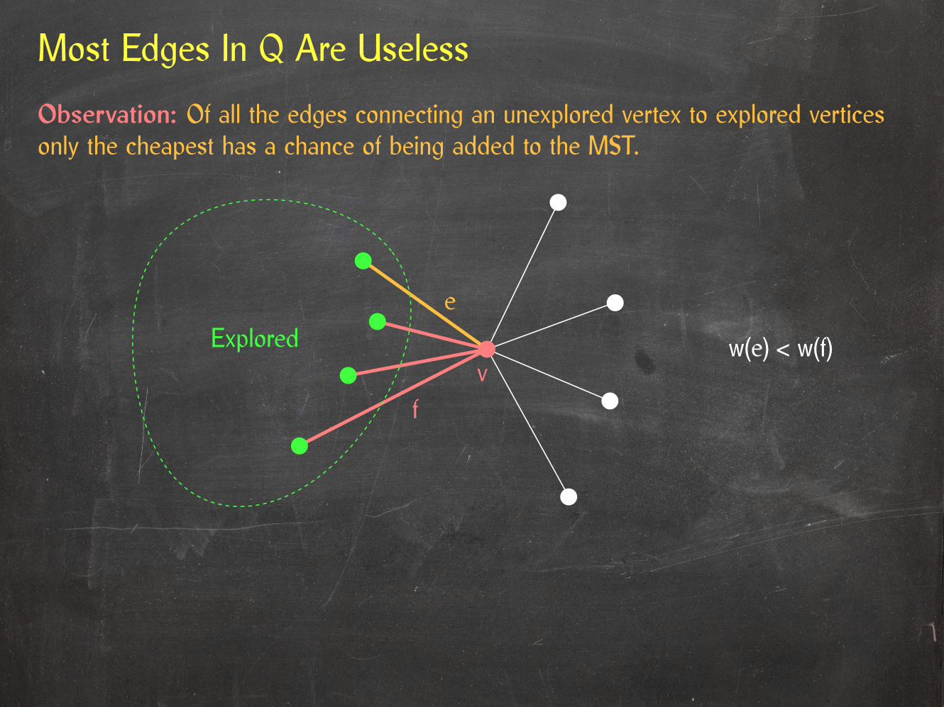
Observation: Of all the edges connecting an unexplored vertex to explored verticesonly the cheapest has a chance of being added to the MST.
w(e) < w(f)Explorede
fv
Most Edges In Q Are Useless
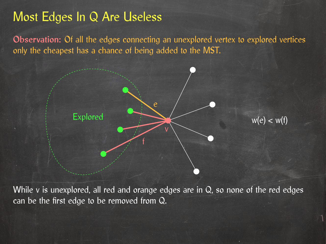
Observation: Of all the edges connecting an unexplored vertex to explored verticesonly the cheapest has a chance of being added to the MST.
While v is unexplored, all red and orange edges are in Q, so none of the red edgescan be the first edge to be removed from Q.
w(e) < w(f)Explorede
fv

Most Edges In Q Are Useless
e
Observation: Of all the edges connecting an unexplored vertex to explored verticesonly the cheapest has a chance of being added to the MST.
While v is unexplored, all red and orange edges are in Q, so none of the red edgescan be the first edge to be removed from Q.
After marking v as explored, both endpoints of red edges are explored, so they cannotbe added to T either.
w(e) < w(f)Explored
fv

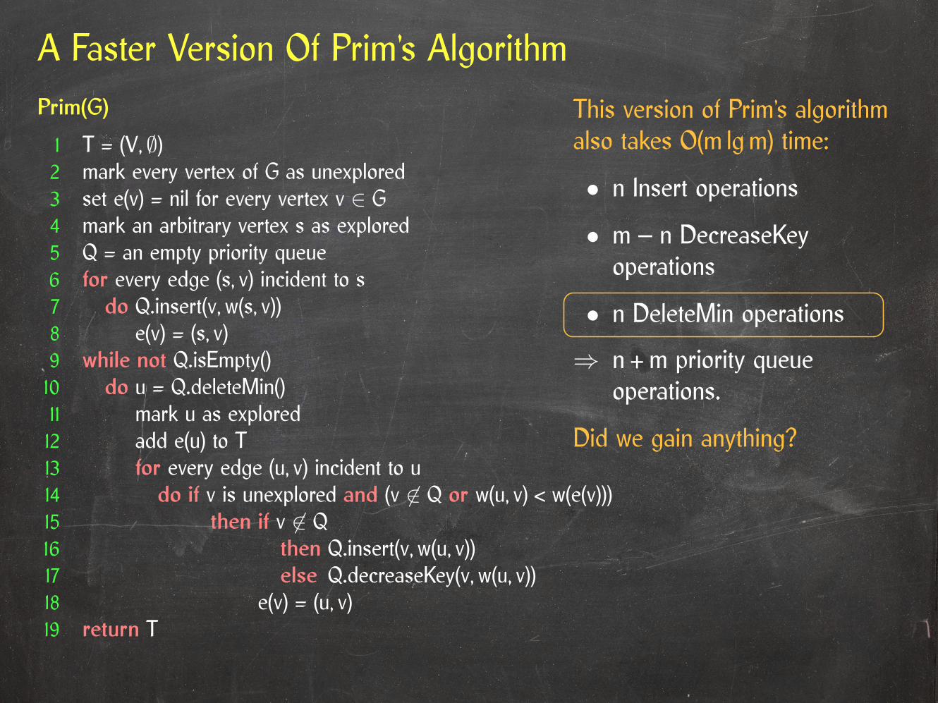
A Faster Version Of Prim’s AlgorithmPrim(G)
1 T = (V, ∅)2 mark every vertex of G as unexplored3 set e(v) = nil for every vertex v ∈ G4 mark an arbitrary vertex s as explored5 Q = an empty priority queue6 for every edge (s, v) incident to s7 do Q.insert(v, w(s, v))8 e(v) = (s, v)9 while not Q.isEmpty()10 do u = Q.deleteMin()11 mark u as explored12 add e(u) to T13 for every edge (u, v) incident to u14 do if v is unexplored and (v 6∈ Q or w(u, v) < w(e(v)))15 then if v 6∈ Q16 then Q.insert(v, w(u, v))17 else Q.decreaseKey(v, w(u, v))18 e(v) = (u, v)19 return T
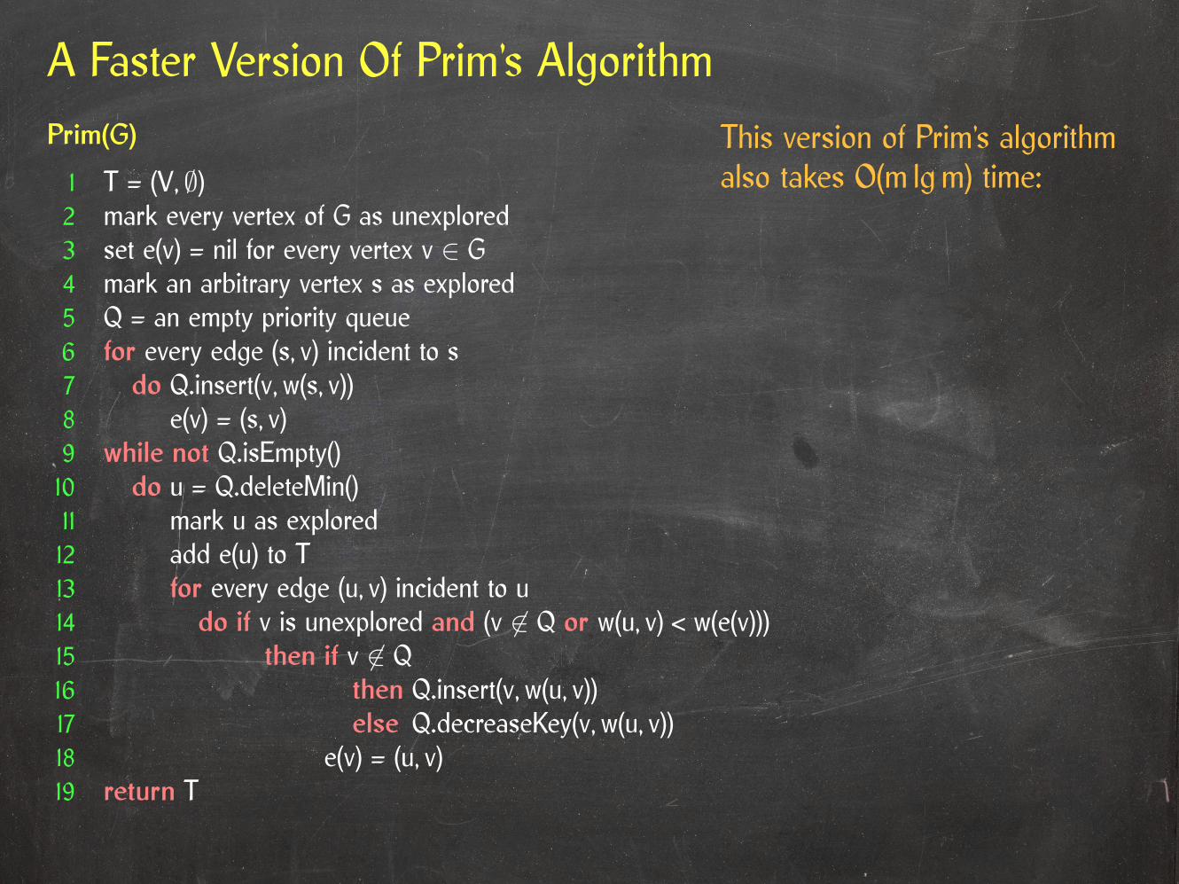
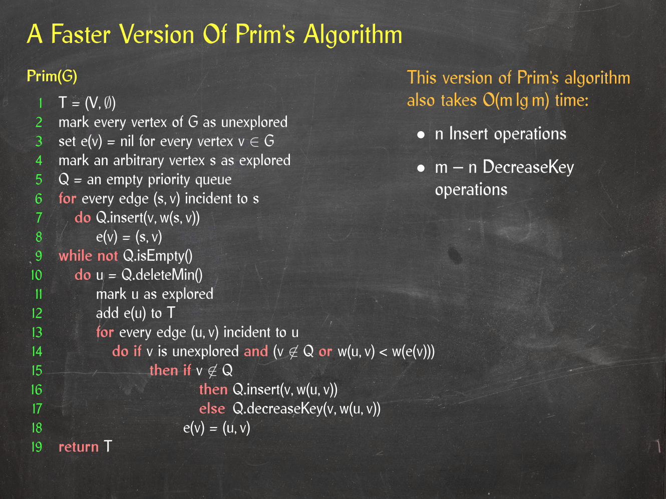
This version of Prim’s algorithmalso takes O(m lgm) time:

A Faster Version Of Prim’s AlgorithmPrim(G)
1 T = (V, ∅)2 mark every vertex of G as unexplored3 set e(v) = nil for every vertex v ∈ G4 mark an arbitrary vertex s as explored5 Q = an empty priority queue6 for every edge (s, v) incident to s7 do Q.insert(v, w(s, v))8 e(v) = (s, v)9 while not Q.isEmpty()10 do u = Q.deleteMin()11 mark u as explored12 add e(u) to T13 for every edge (u, v) incident to u14 do if v is unexplored and (v 6∈ Q or w(u, v) < w(e(v)))15 then if v 6∈ Q16 then Q.insert(v, w(u, v))17 else Q.decreaseKey(v, w(u, v))18 e(v) = (u, v)19 return T
This version of Prim’s algorithmalso takes O(m lgm) time:
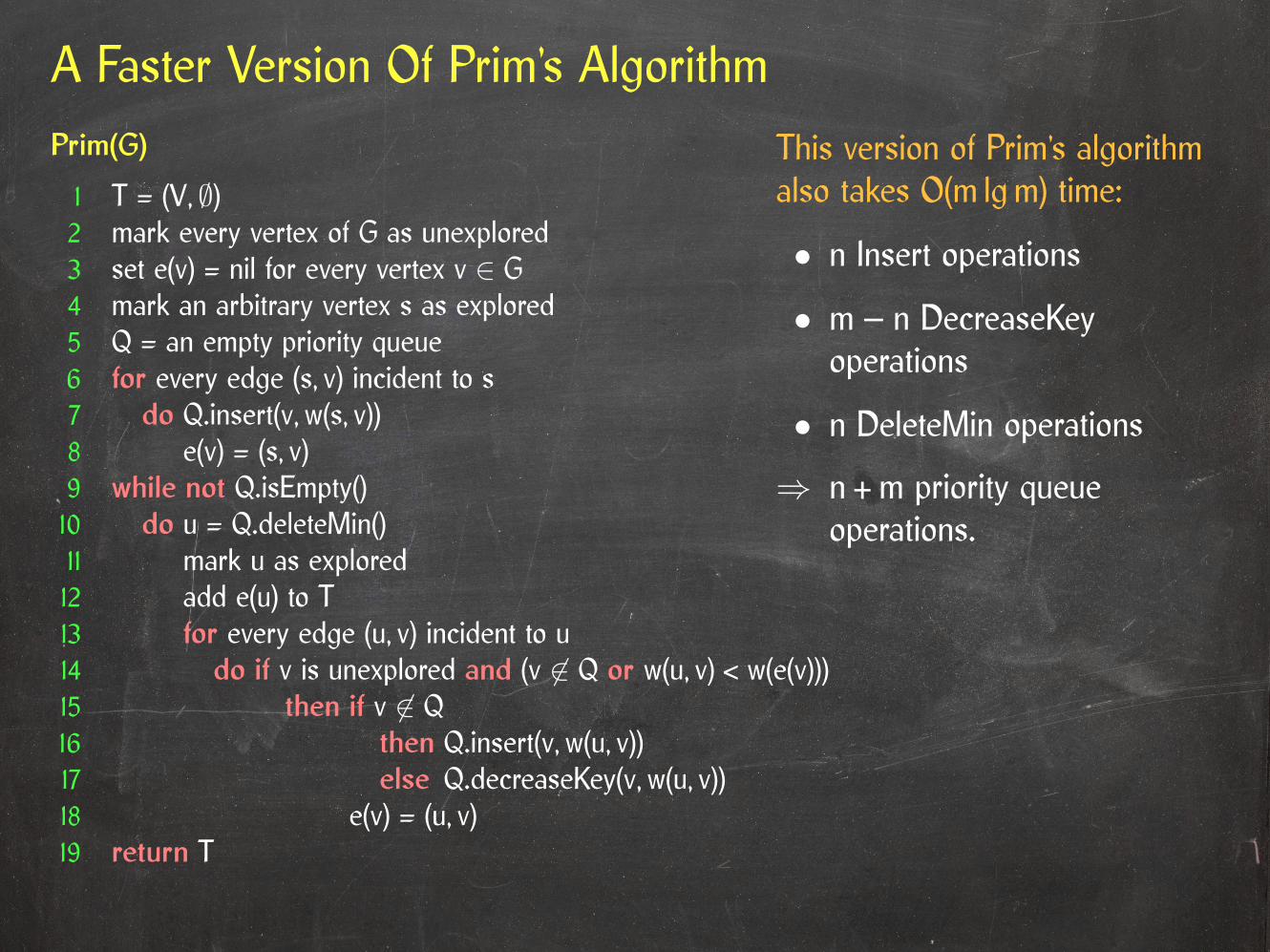
• n Insert operations
A Faster Version Of Prim’s AlgorithmPrim(G)
1 T = (V, ∅)2 mark every vertex of G as unexplored3 set e(v) = nil for every vertex v ∈ G4 mark an arbitrary vertex s as explored5 Q = an empty priority queue6 for every edge (s, v) incident to s7 do Q.insert(v, w(s, v))8 e(v) = (s, v)9 while not Q.isEmpty()10 do u = Q.deleteMin()11 mark u as explored12 add e(u) to T13 for every edge (u, v) incident to u14 do if v is unexplored and (v 6∈ Q or w(u, v) < w(e(v)))15 then if v 6∈ Q16 then Q.insert(v, w(u, v))17 else Q.decreaseKey(v, w(u, v))18 e(v) = (u, v)19 return T
This version of Prim’s algorithmalso takes O(m lgm) time:
• n Insert operations
• m – n DecreaseKeyoperations
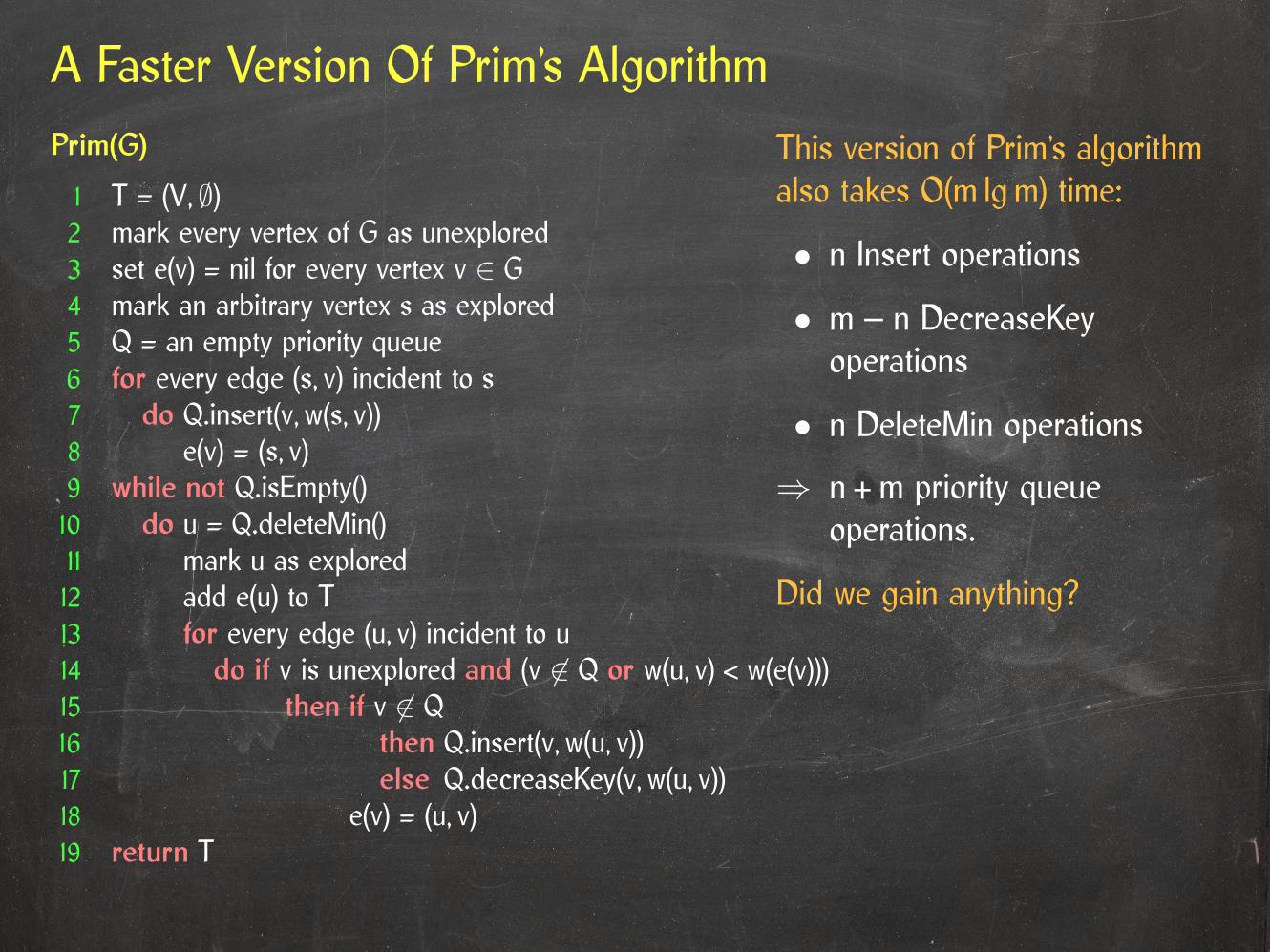
• n DeleteMin operations
A Faster Version Of Prim’s AlgorithmPrim(G)
1 T = (V, ∅)2 mark every vertex of G as unexplored3 set e(v) = nil for every vertex v ∈ G4 mark an arbitrary vertex s as explored5 Q = an empty priority queue6 for every edge (s, v) incident to s7 do Q.insert(v, w(s, v))8 e(v) = (s, v)9 while not Q.isEmpty()10 do u = Q.deleteMin()11 mark u as explored12 add e(u) to T13 for every edge (u, v) incident to u14 do if v is unexplored and (v 6∈ Q or w(u, v) < w(e(v)))15 then if v 6∈ Q16 then Q.insert(v, w(u, v))17 else Q.decreaseKey(v, w(u, v))18 e(v) = (u, v)19 return T
This version of Prim’s algorithmalso takes O(m lgm) time:
• n Insert operations
• m – n DecreaseKeyoperations
⇒ n + m priority queueoperations.
• n DeleteMin operations
Did we gain anything?

Thin Heap
The Thin Heap is a priority queue which supports
• Insert, DecreaseKey, and FindMin in O(1) time and• DeleteMin and Delete in O(lg n) time.

Thin Heap
The Thin Heap is a priority queue which supports
• Insert, DecreaseKey, and FindMin in O(1) time and• DeleteMin and Delete in O(lg n) time.
These bounds are amortized:
• Individual operations can take much longer.• A sequence of m operations, d of them DeleteMin or Delete operations, takesO(m + d lg n) time in the worst case.
Prim’s algorithm performs n + m priority queue operations, n of which are DeleteMinoperations.
Lemma: Prim’s algorithm takes O(n lg n + m) time.
Thin Tree
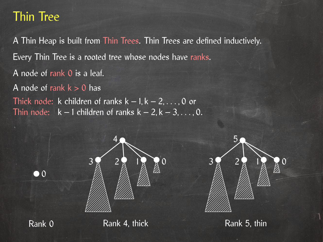
A Thin Heap is built from Thin Trees. Thin Trees are defined inductively.

Thin Tree
A Thin Heap is built from Thin Trees. Thin Trees are defined inductively.
Every Thin Tree is a rooted tree whose nodes have ranks.
Thin Tree
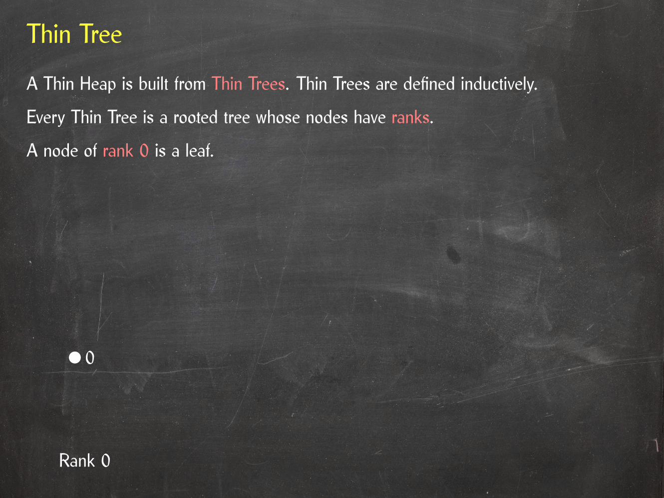
A Thin Heap is built from Thin Trees. Thin Trees are defined inductively.
Every Thin Tree is a rooted tree whose nodes have ranks.
A node of rank 0 is a leaf.
Rank 0
0
Thin Tree
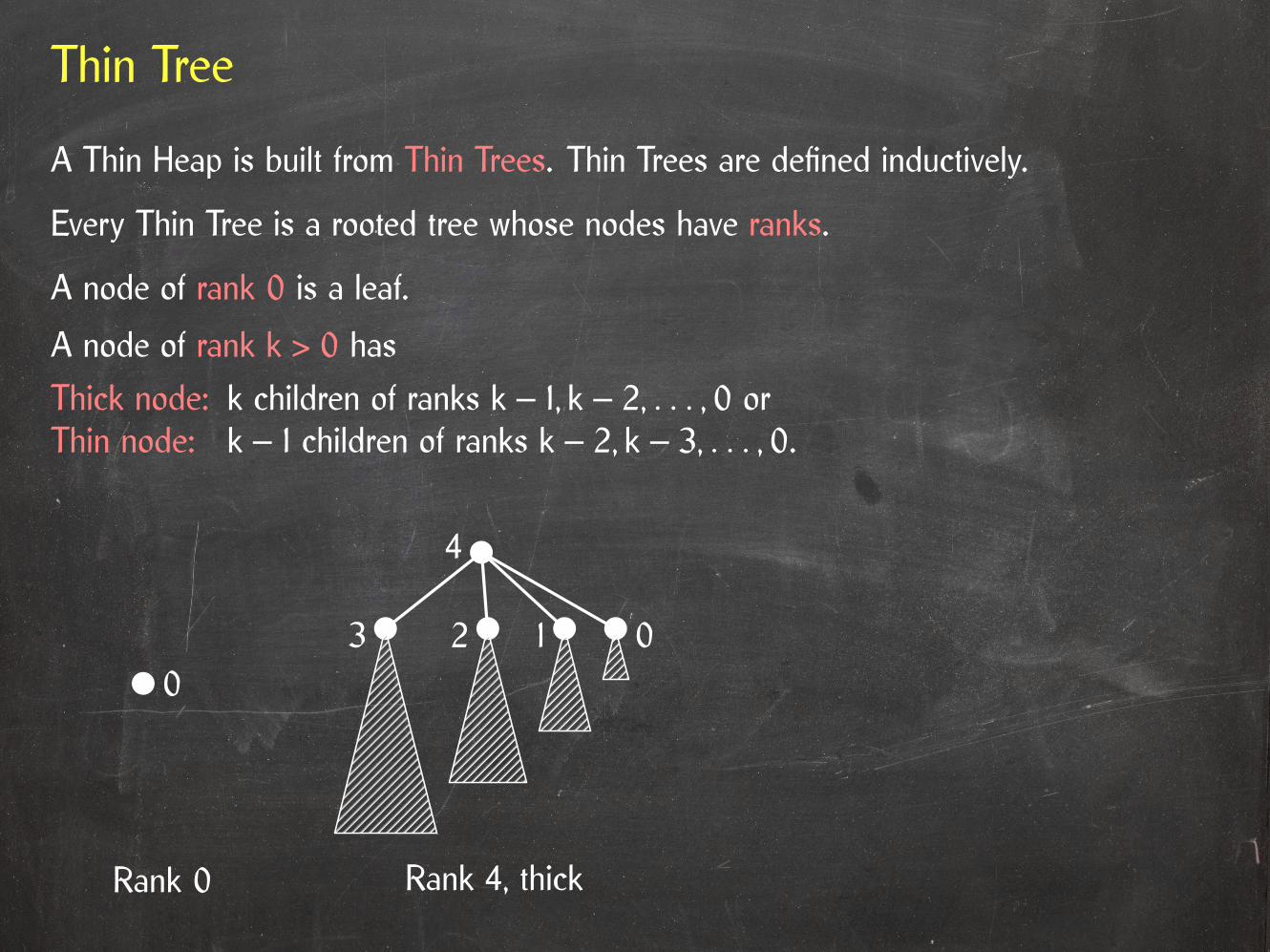
A Thin Heap is built from Thin Trees. Thin Trees are defined inductively.
Every Thin Tree is a rooted tree whose nodes have ranks.
A node of rank 0 is a leaf.
A node of rank k > 0 has
Thick node: k children of ranks k – 1, k – 2, . . . , 0 orThin node: k – 1 children of ranks k – 2, k – 3, . . . , 0.
Rank 0
0
Rank 4, thick
3 2 1 0
4
Thin Tree
A Thin Heap is built from Thin Trees. Thin Trees are defined inductively.
Every Thin Tree is a rooted tree whose nodes have ranks.
A node of rank 0 is a leaf.
A node of rank k > 0 has
Thick node: k children of ranks k – 1, k – 2, . . . , 0 orThin node: k – 1 children of ranks k – 2, k – 3, . . . , 0.
Rank 0
0
Rank 4, thick
3 2 1 0
4
Rank 5, thin
3 2 1 0
5
Thin Heap
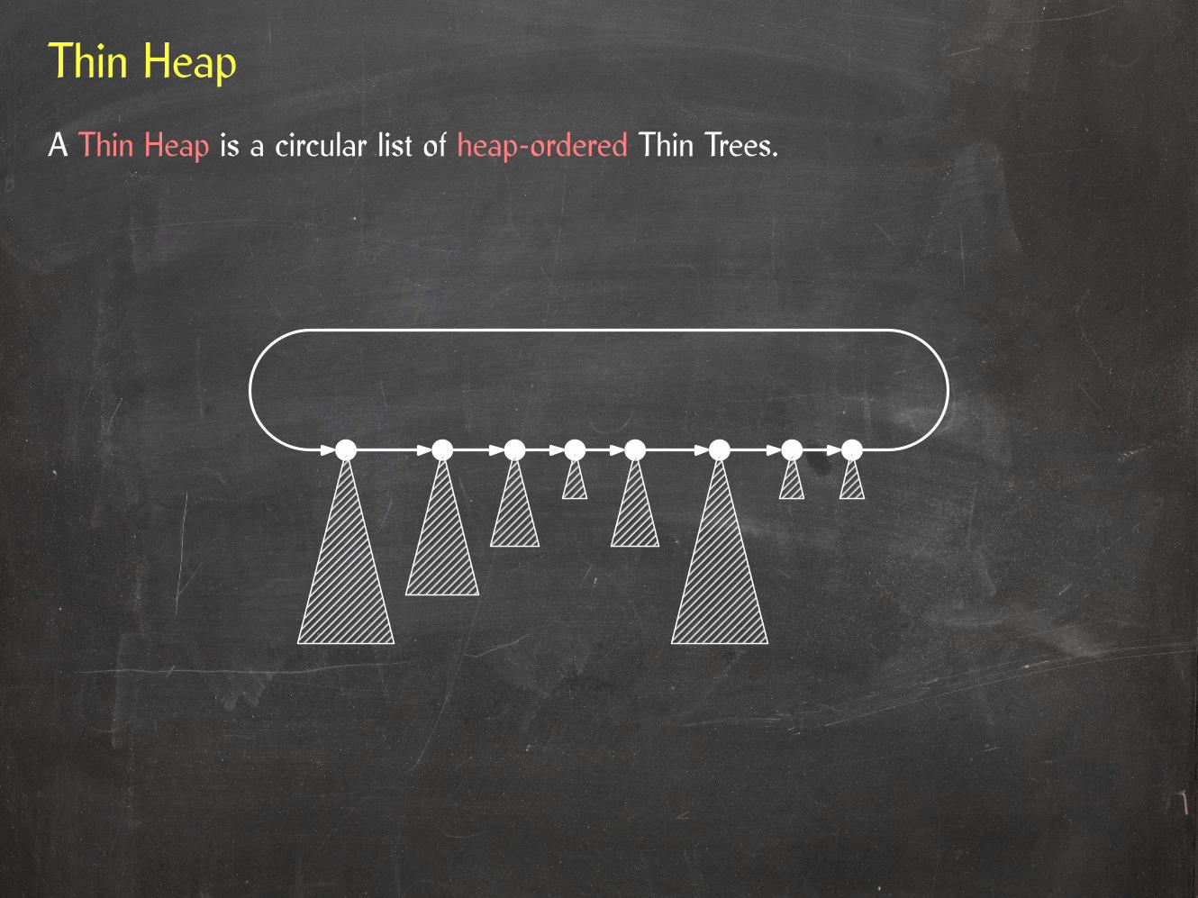
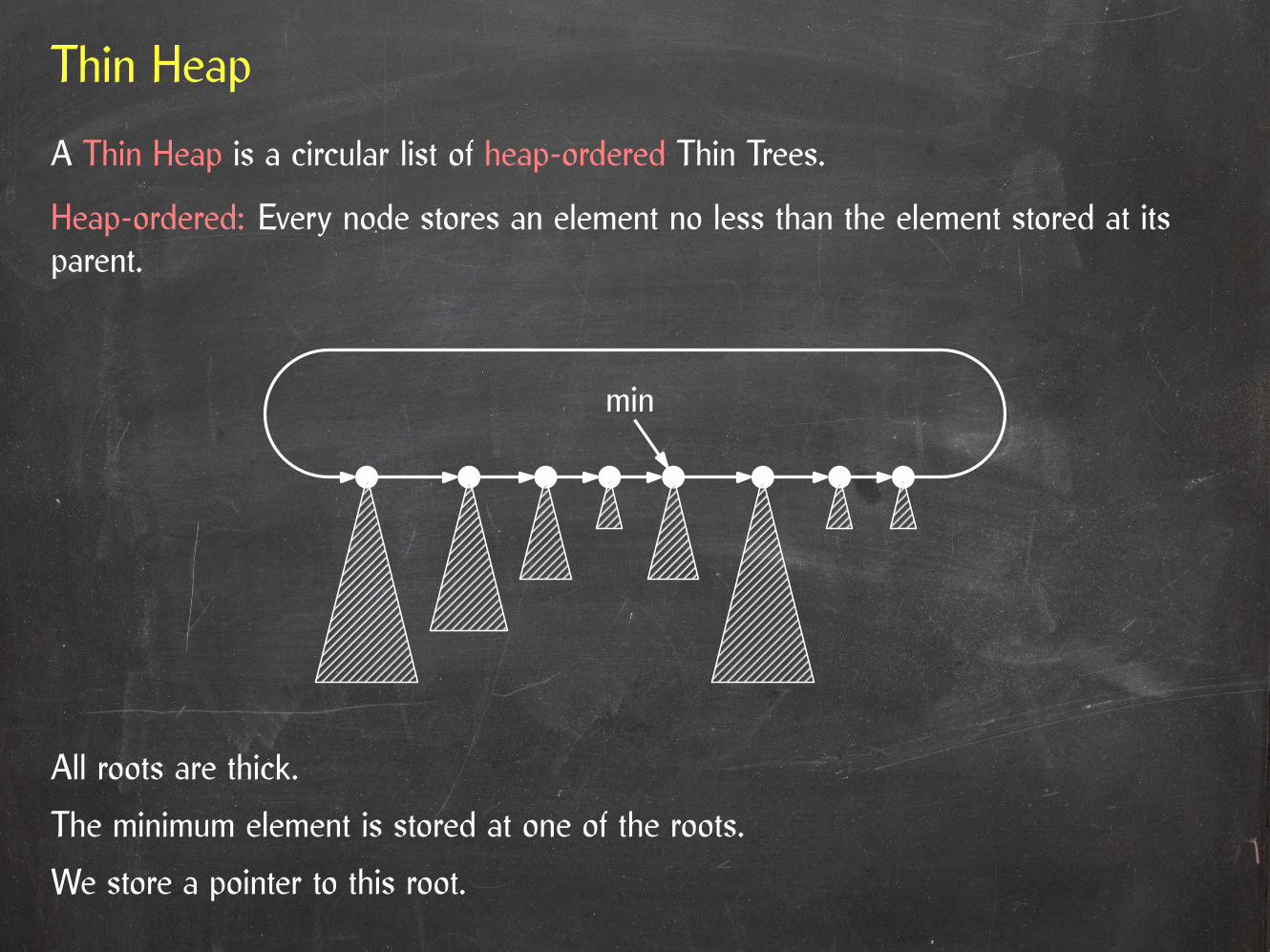
A Thin Heap is a circular list of heap-ordered Thin Trees.
Thin Heap
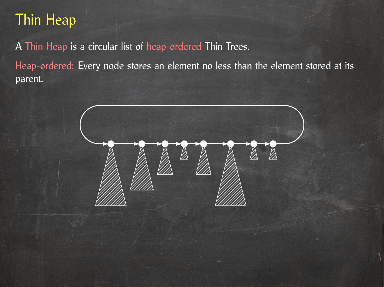
A Thin Heap is a circular list of heap-ordered Thin Trees.
Heap-ordered: Every node stores an element no less than the element stored at itsparent.

Thin Heap
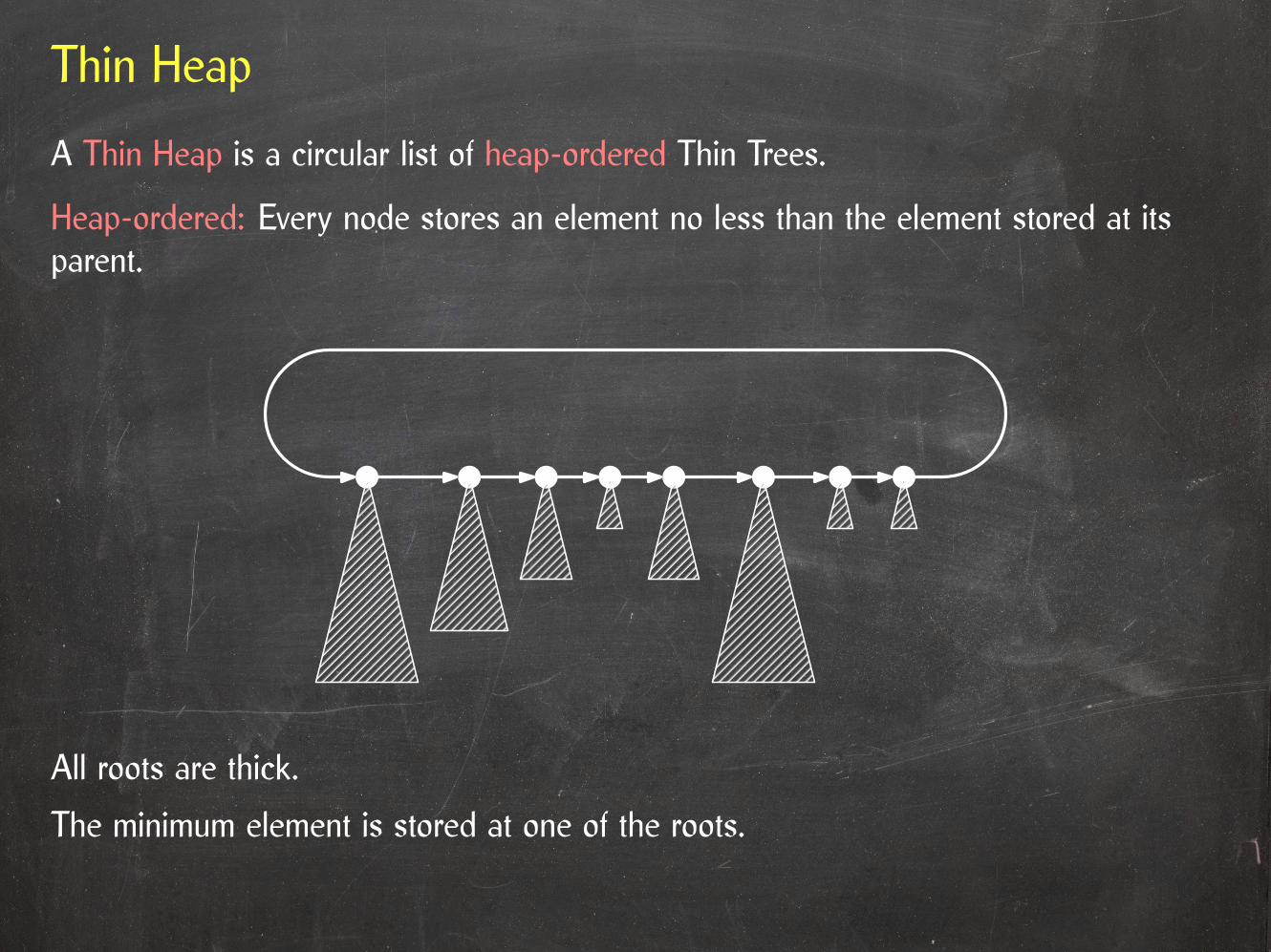
All roots are thick.
A Thin Heap is a circular list of heap-ordered Thin Trees.
Heap-ordered: Every node stores an element no less than the element stored at itsparent.
Thin Heap
All roots are thick.
The minimum element is stored at one of the roots.
A Thin Heap is a circular list of heap-ordered Thin Trees.
Heap-ordered: Every node stores an element no less than the element stored at itsparent.
Thin Heap
min
All roots are thick.
The minimum element is stored at one of the roots.
We store a pointer to this root.
A Thin Heap is a circular list of heap-ordered Thin Trees.
Heap-ordered: Every node stores an element no less than the element stored at itsparent.

Node Representation
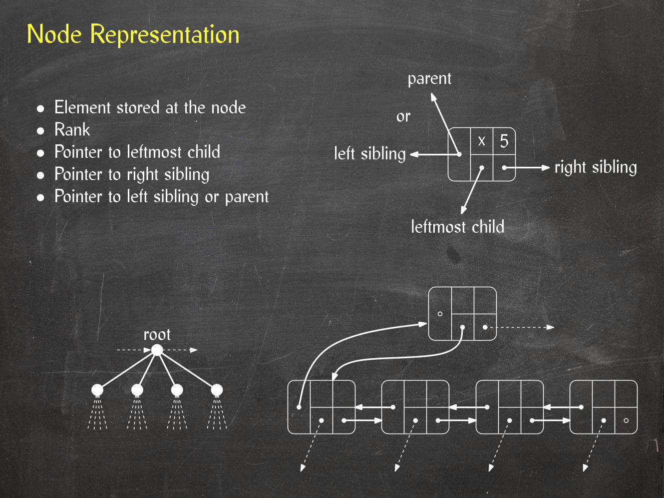
• Element stored at the node• Rank• Pointer to leftmost child• Pointer to right sibling• Pointer to left sibling or parent
x 5or
parent
left siblingright sibling
leftmost child
Node Representation
• Element stored at the node• Rank• Pointer to leftmost child• Pointer to right sibling• Pointer to left sibling or parent
x 5or
parent
left siblingright sibling
leftmost child
root

FindMin
... is easy:
min
Delete
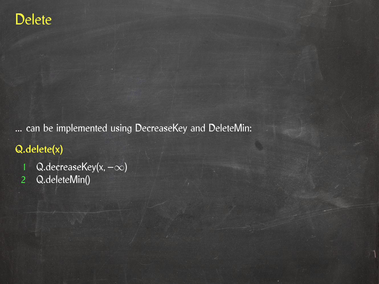
... can be implemented using DecreaseKey and DeleteMin:
Q.delete(x)
1 Q.decreaseKey(x, –∞)2 Q.deleteMin()
Insert
Insert
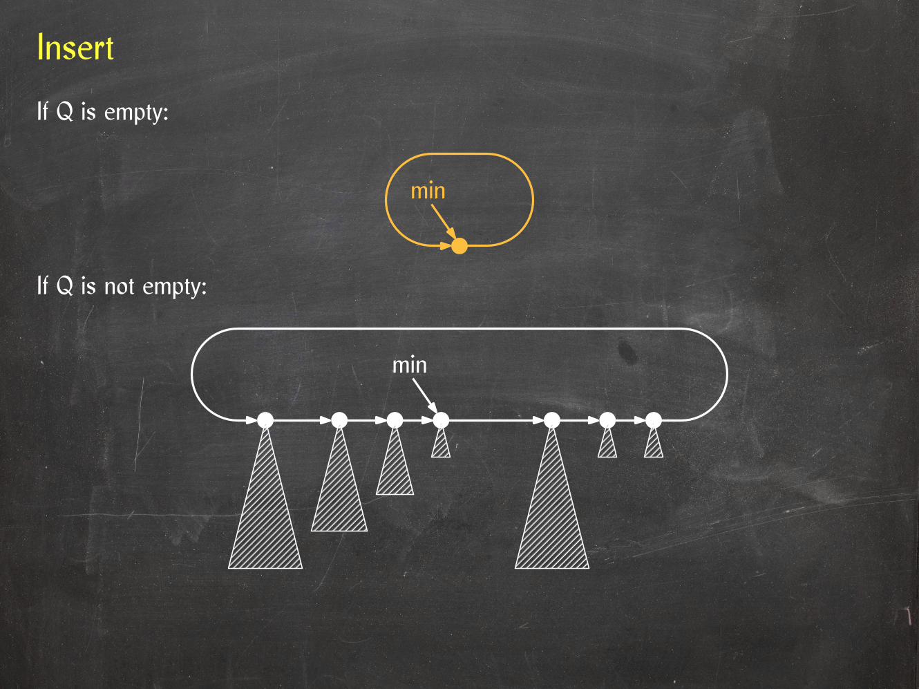
If Q is empty:

Insert
If Q is empty:
min
Insert
If Q is empty:
If Q is not empty:
min
min

Insert
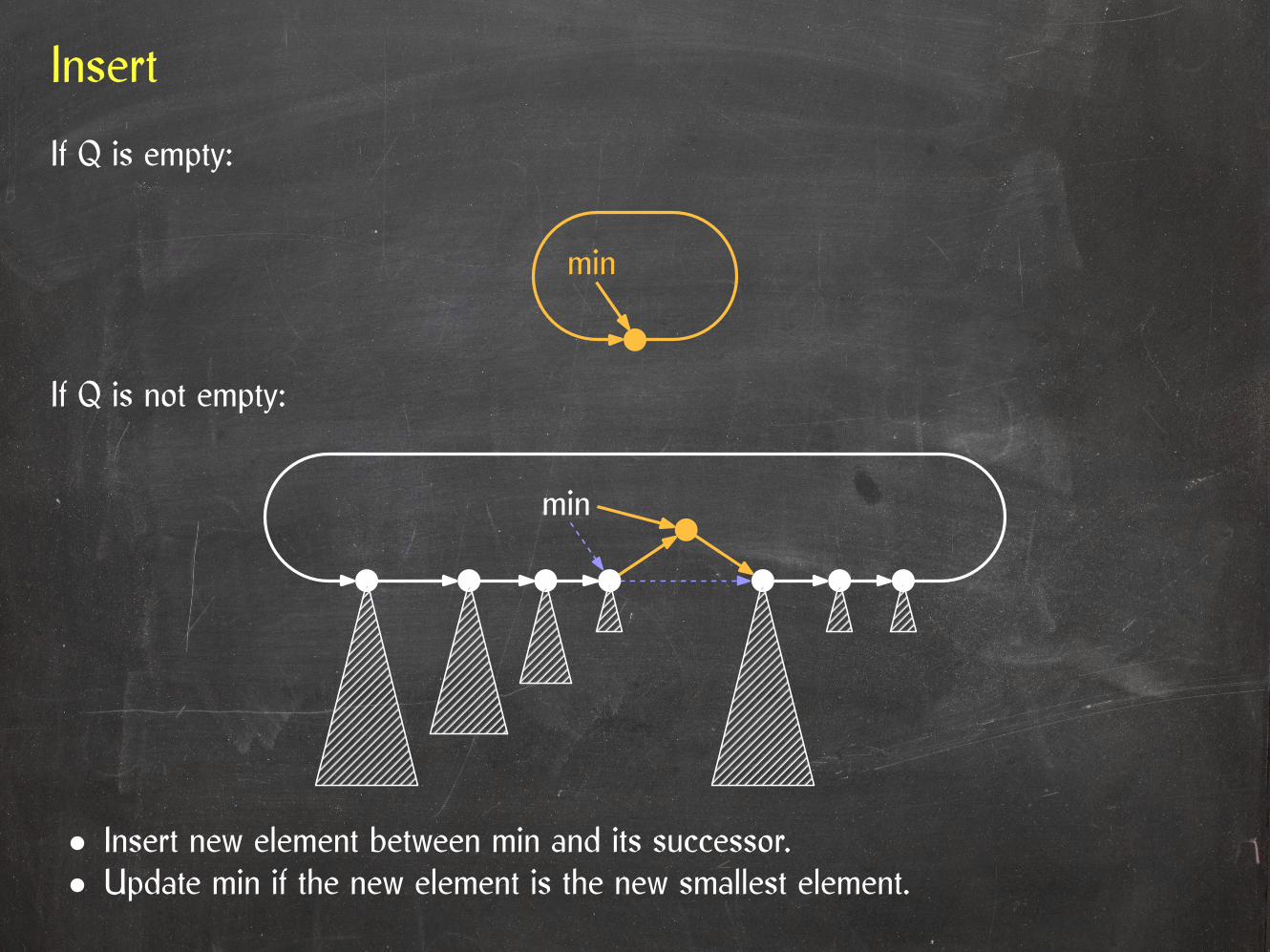
If Q is empty:
If Q is not empty:
• Insert new element between min and its successor.
min
min
Insert
If Q is empty:
If Q is not empty:
• Insert new element between min and its successor.• Update min if the new element is the new smallest element.
min
min

DeleteMin
min
DeleteMin
min

DeleteMin
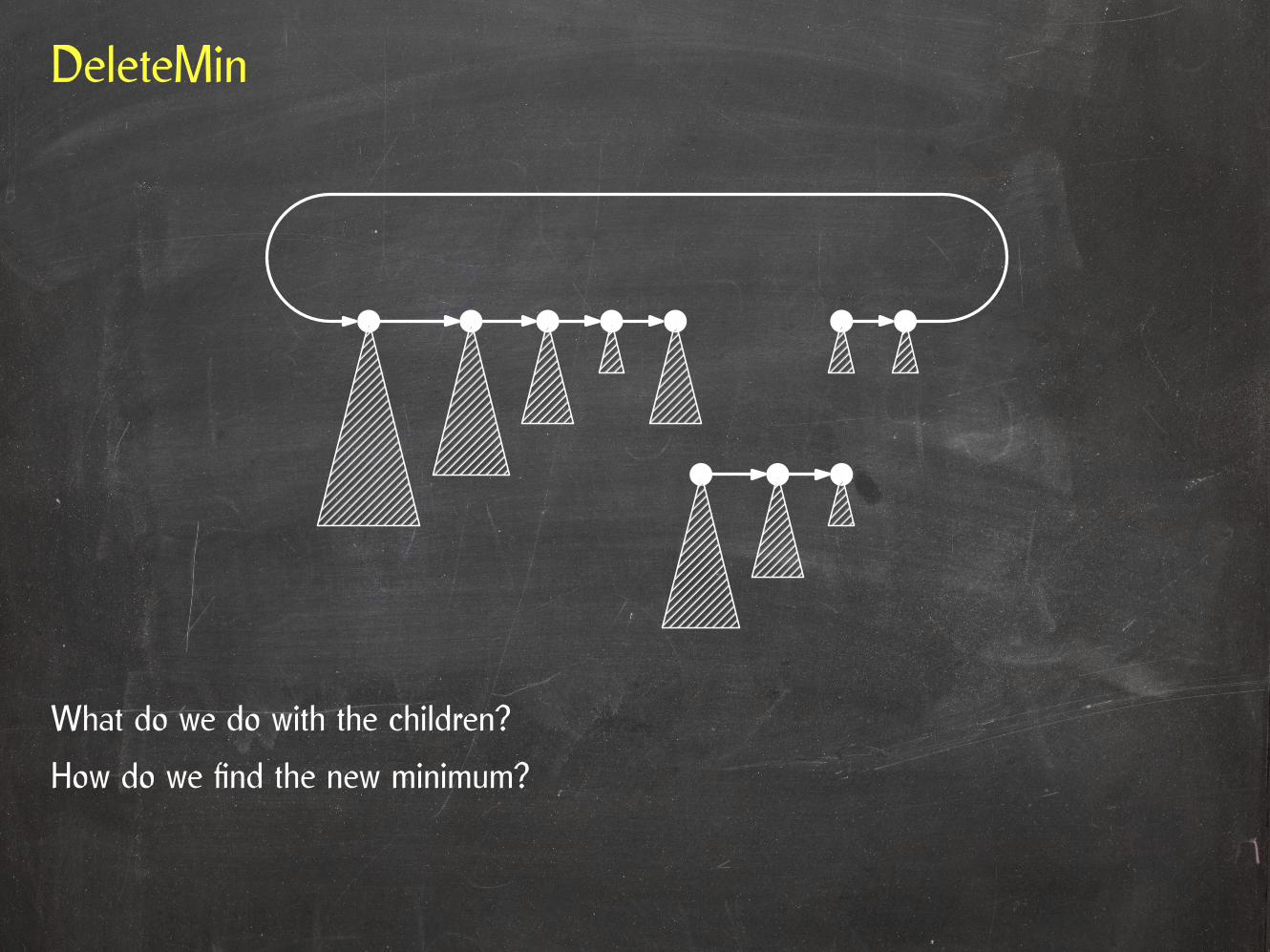
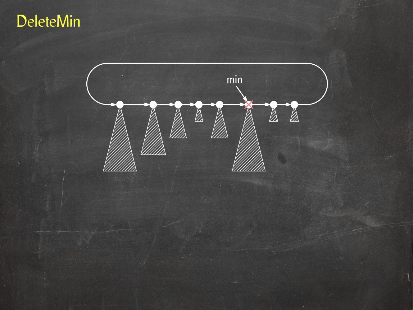
DeleteMin
What do we do with the children?
How do we find the new minimum?

DeleteMin
How do we find the new minimum?• Could be one of the children.• Could be one of the other roots.
What do we do with the children?

DeleteMin
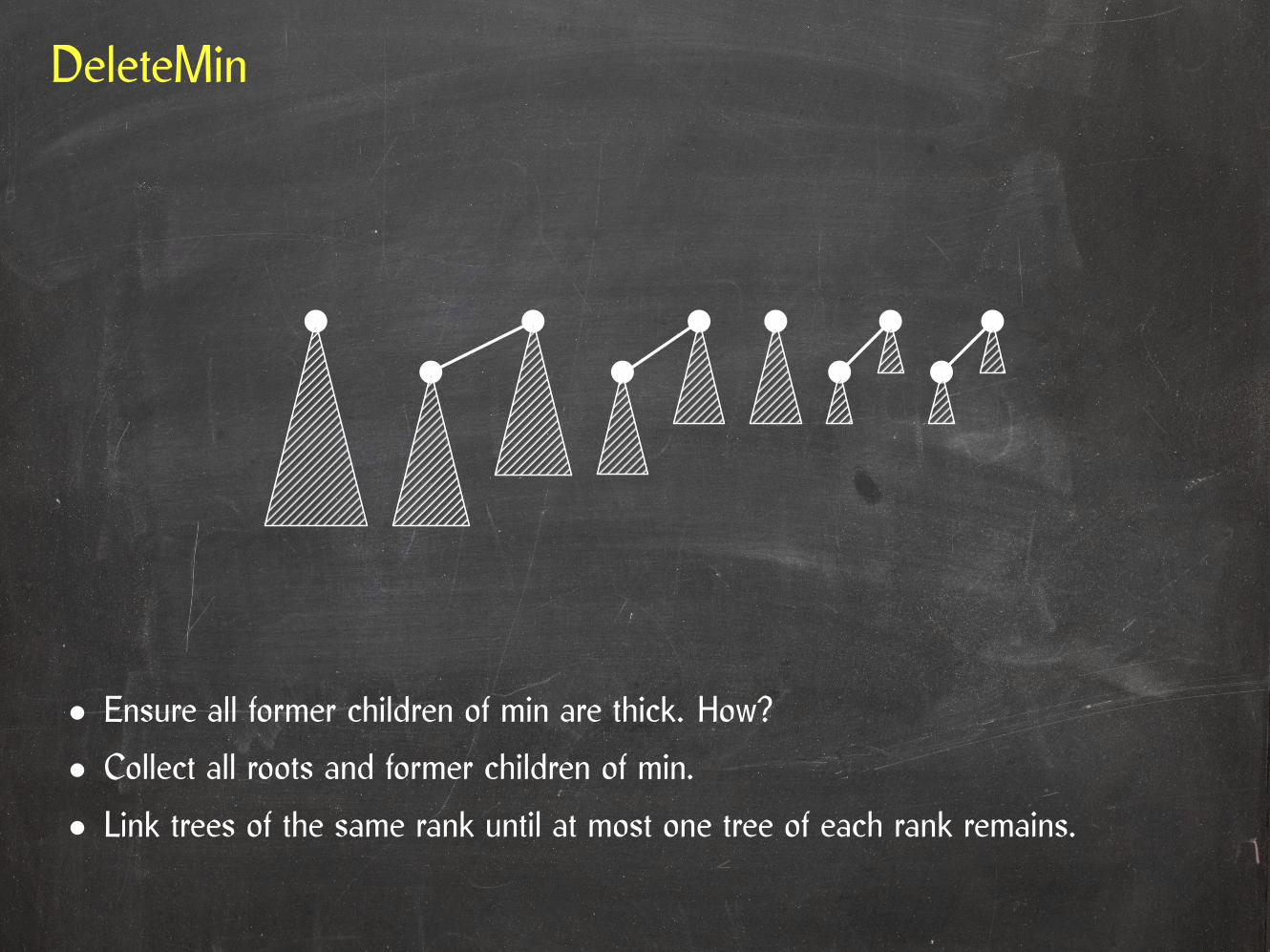
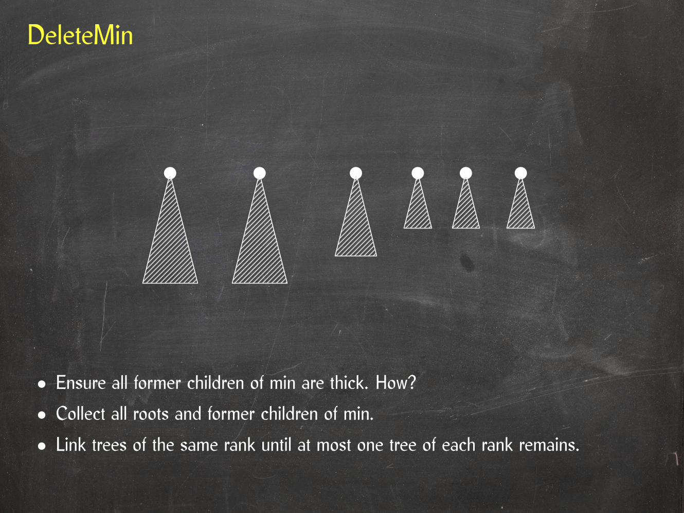
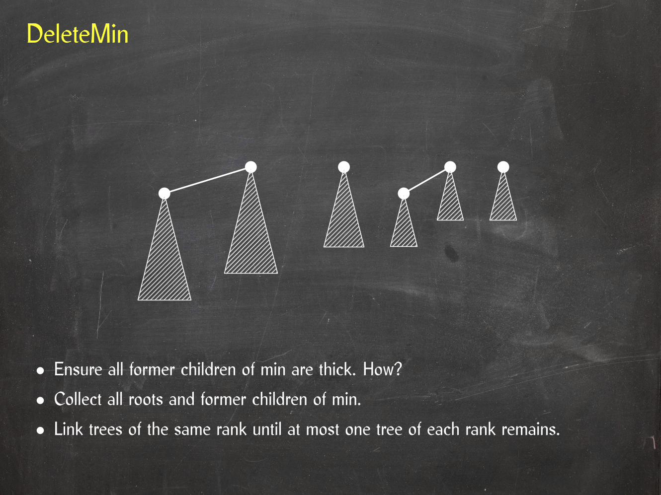
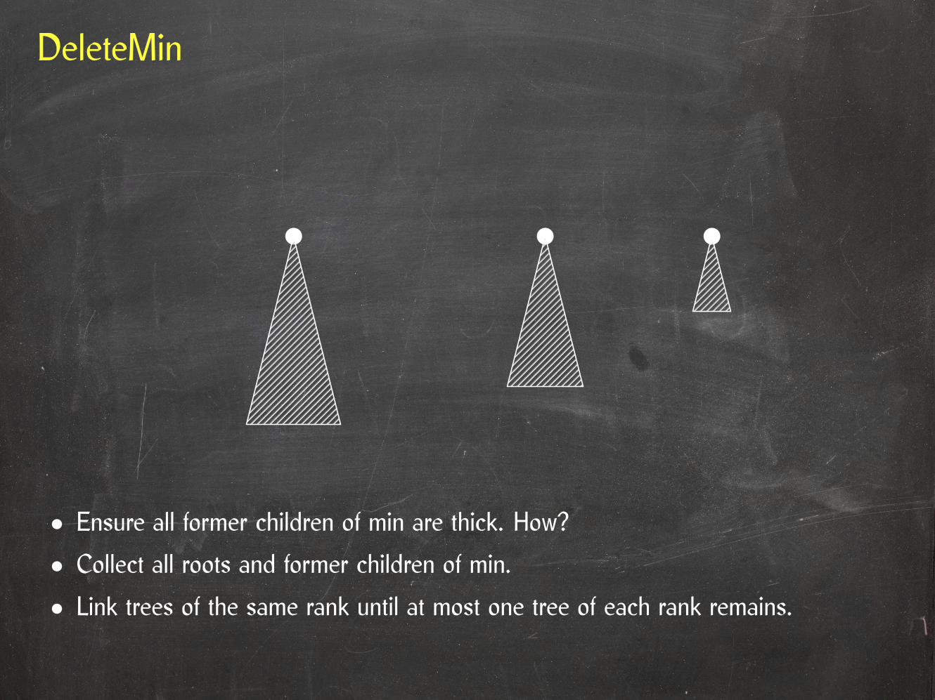
• Ensure all former children of min are thick. How?

DeleteMin
• Ensure all former children of min are thick. How?
• Collect all roots and former children of min.
DeleteMin
• Ensure all former children of min are thick. How?
• Collect all roots and former children of min.
• Link trees of the same rank until at most one tree of each rank remains.
DeleteMin
• Ensure all former children of min are thick. How?
• Collect all roots and former children of min.
• Link trees of the same rank until at most one tree of each rank remains.
DeleteMin
• Ensure all former children of min are thick. How?
• Collect all roots and former children of min.
• Link trees of the same rank until at most one tree of each rank remains.

DeleteMin
• Ensure all former children of min are thick. How?
• Collect all roots and former children of min.
• Link trees of the same rank until at most one tree of each rank remains.

DeleteMin
• Ensure all former children of min are thick. How?
• Collect all roots and former children of min.
• Link trees of the same rank until at most one tree of each rank remains.
DeleteMin
• Ensure all former children of min are thick. How?
• Collect all roots and former children of min.
• Link trees of the same rank until at most one tree of each rank remains.
DeleteMin
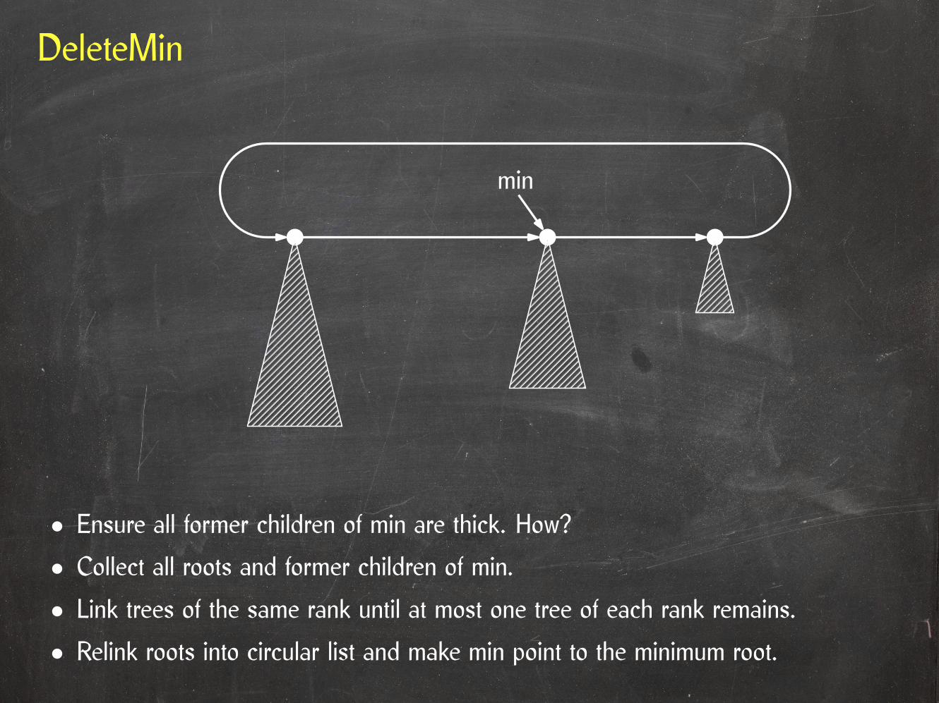
• Ensure all former children of min are thick. How?
• Collect all roots and former children of min.
• Link trees of the same rank until at most one tree of each rank remains.
min
• Relink roots into circular list and make min point to the minimum root.
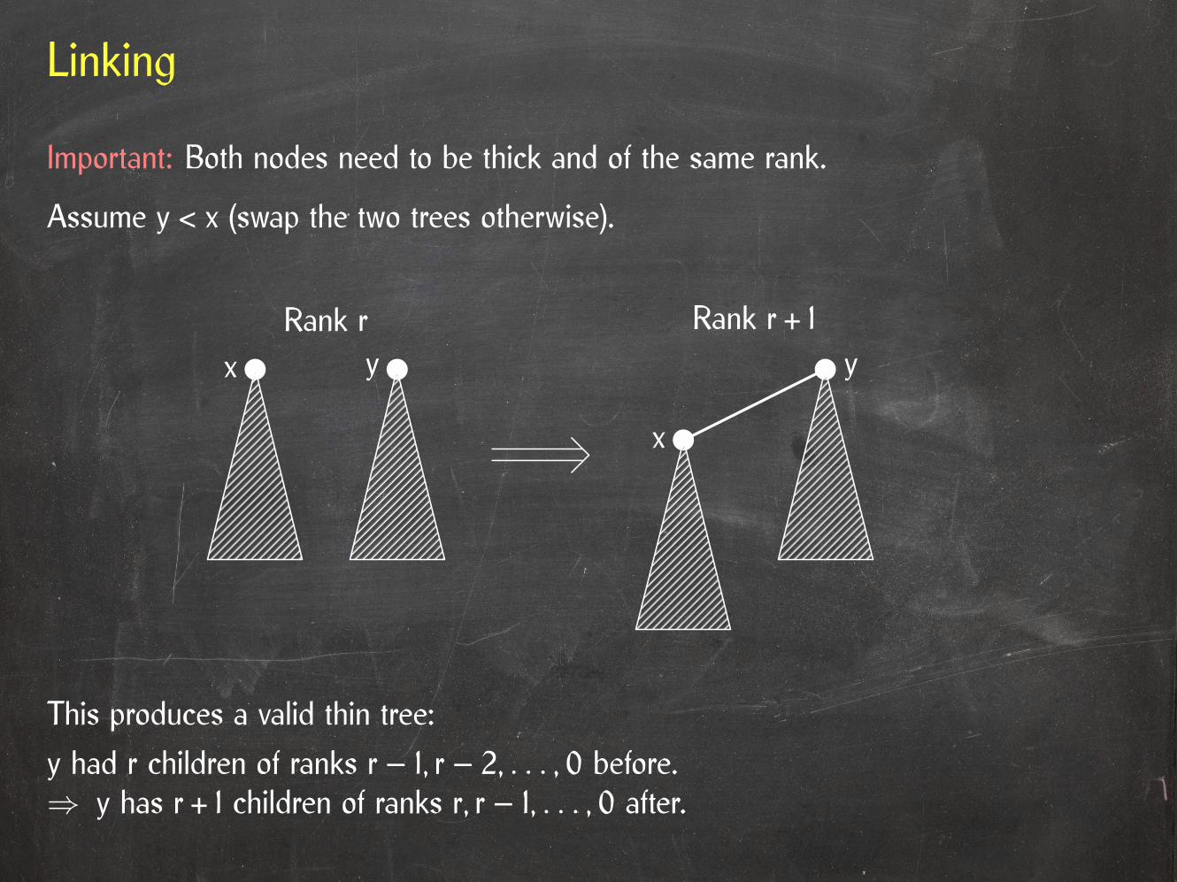
Linking
Rank r Rank r + 1yx
x
y
This produces a valid thin tree:
y had r children of ranks r – 1, r – 2, . . . , 0 before.⇒ y has r + 1 children of ranks r, r – 1, . . . , 0 after.
Important: Both nodes need to be thick and of the same rank.
Assume y < x (swap the two trees otherwise).
Bounding the Maximum Rank
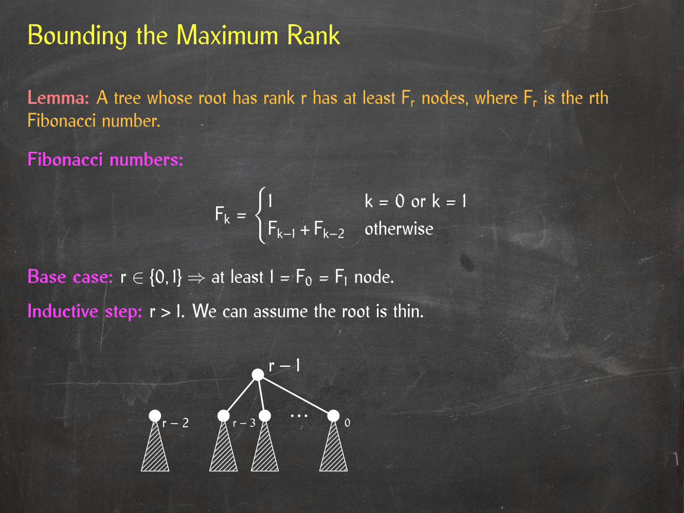
Lemma: A tree whose root has rank r has at least Fr nodes, where Fr is the rthFibonacci number.

Bounding the Maximum Rank
Lemma: A tree whose root has rank r has at least Fr nodes, where Fr is the rthFibonacci number.
Fibonacci numbers:
Fk =
{1 k = 0 or k = 1Fk–1 + Fk–2 otherwise

Bounding the Maximum Rank
Lemma: A tree whose root has rank r has at least Fr nodes, where Fr is the rthFibonacci number.
Fibonacci numbers:
Fk =
{1 k = 0 or k = 1Fk–1 + Fk–2 otherwise
Base case: r ∈ {0, 1}⇒ at least 1 = F0 = F1 node.

Bounding the Maximum Rank
Lemma: A tree whose root has rank r has at least Fr nodes, where Fr is the rthFibonacci number.
Fibonacci numbers:
Fk =
{1 k = 0 or k = 1Fk–1 + Fk–2 otherwise
Base case: r ∈ {0, 1}⇒ at least 1 = F0 = F1 node.
Inductive step: r > 1. We can assume the root is thin.
r
r – 2 r – 3 0
Bounding the Maximum Rank
Lemma: A tree whose root has rank r has at least Fr nodes, where Fr is the rthFibonacci number.
Fibonacci numbers:
Fk =
{1 k = 0 or k = 1Fk–1 + Fk–2 otherwise
Base case: r ∈ {0, 1}⇒ at least 1 = F0 = F1 node.
Inductive step: r > 1. We can assume the root is thin.
r – 1
r – 2 r – 3 0

Bounding the Maximum Rank
Lemma: A tree whose root has rank r has at least Fr nodes, where Fr is the rthFibonacci number.
Fibonacci numbers:
Fk =
{1 k = 0 or k = 1Fk–1 + Fk–2 otherwise
Base case: r ∈ {0, 1}⇒ at least 1 = F0 = F1 node.
Inductive step: r > 1. We can assume the root is thin.
Fr–1 + Fr–2 = Fr
r – 1
r – 2 r – 3 0
≥ Fr–2 ≥ Fr–1
Bounding the Maximum Rank
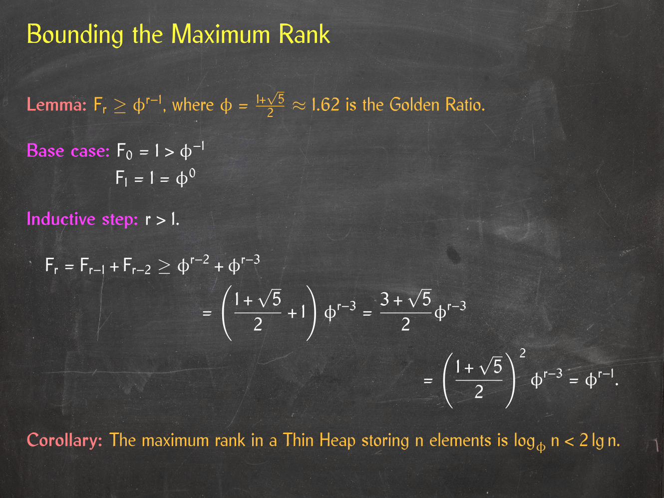
Lemma: Fr ≥ φr–1, where φ = 1+√5
2 ≈ 1.62 is the Golden Ratio.
Bounding the Maximum Rank
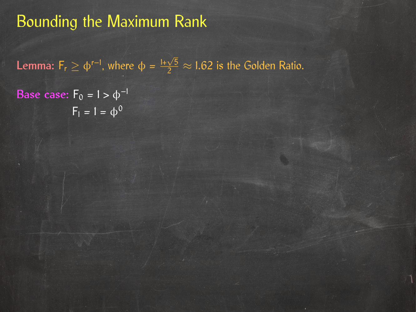
Lemma: Fr ≥ φr–1, where φ = 1+√5
2 ≈ 1.62 is the Golden Ratio.
Base case: F0 = 1 > φ–1
F1 = 1 = φ0
Bounding the Maximum Rank
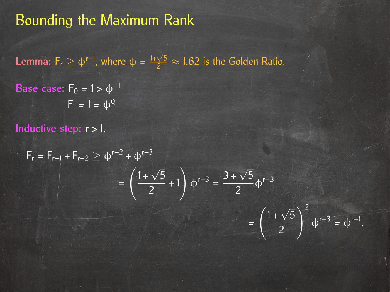
Lemma: Fr ≥ φr–1, where φ = 1+√5
2 ≈ 1.62 is the Golden Ratio.
Base case: F0 = 1 > φ–1
F1 = 1 = φ0
Inductive step: r > 1.
Fr = Fr–1 + Fr–2 ≥ φr–2 + φr–3
=
(1 +√5
2+ 1
)φr–3 =
3 +√5
2φr–3
=
(1 +√5
2
)2
φr–3 = φr–1.
Bounding the Maximum Rank
Lemma: Fr ≥ φr–1, where φ = 1+√5
2 ≈ 1.62 is the Golden Ratio.
Base case: F0 = 1 > φ–1
F1 = 1 = φ0
Inductive step: r > 1.
Fr = Fr–1 + Fr–2 ≥ φr–2 + φr–3
=
(1 +√5
2+ 1
)φr–3 =
3 +√5
2φr–3
=
(1 +√5
2
)2
φr–3 = φr–1.
Corollary: The maximum rank in a Thin Heap storing n elements is logφ n < 2 lg n.

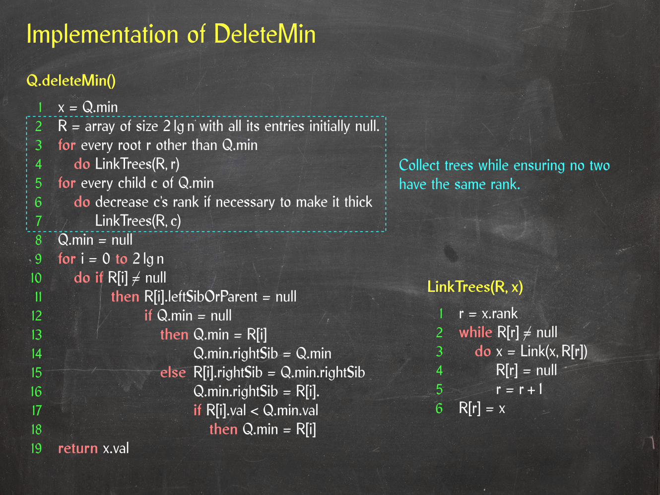
Implementation of DeleteMin
Q.deleteMin()
1 x = Q.min2 R = array of size 2 lg n with all its entries initially null.3 for every root r other than Q.min4 do LinkTrees(R, r)5 for every child c of Q.min6 do decrease c’s rank if necessary to make it thick7 LinkTrees(R, c)8 Q.min = null9 for i = 0 to 2 lg n10 do if R[i] 6= null11 then R[i].leftSibOrParent = null12 if Q.min = null13 then Q.min = R[i]14 Q.min.rightSib = Q.min15 else R[i].rightSib = Q.min.rightSib16 Q.min.rightSib = R[i].17 if R[i].val < Q.min.val18 then Q.min = R[i]19 return x.val
Collect trees while ensuring no twohave the same rank.
LinkTrees(R, x)
1 r = x.rank2 while R[r] 6= null3 do x = Link(x, R[r])4 R[r] = null5 r = r + 16 R[r] = x
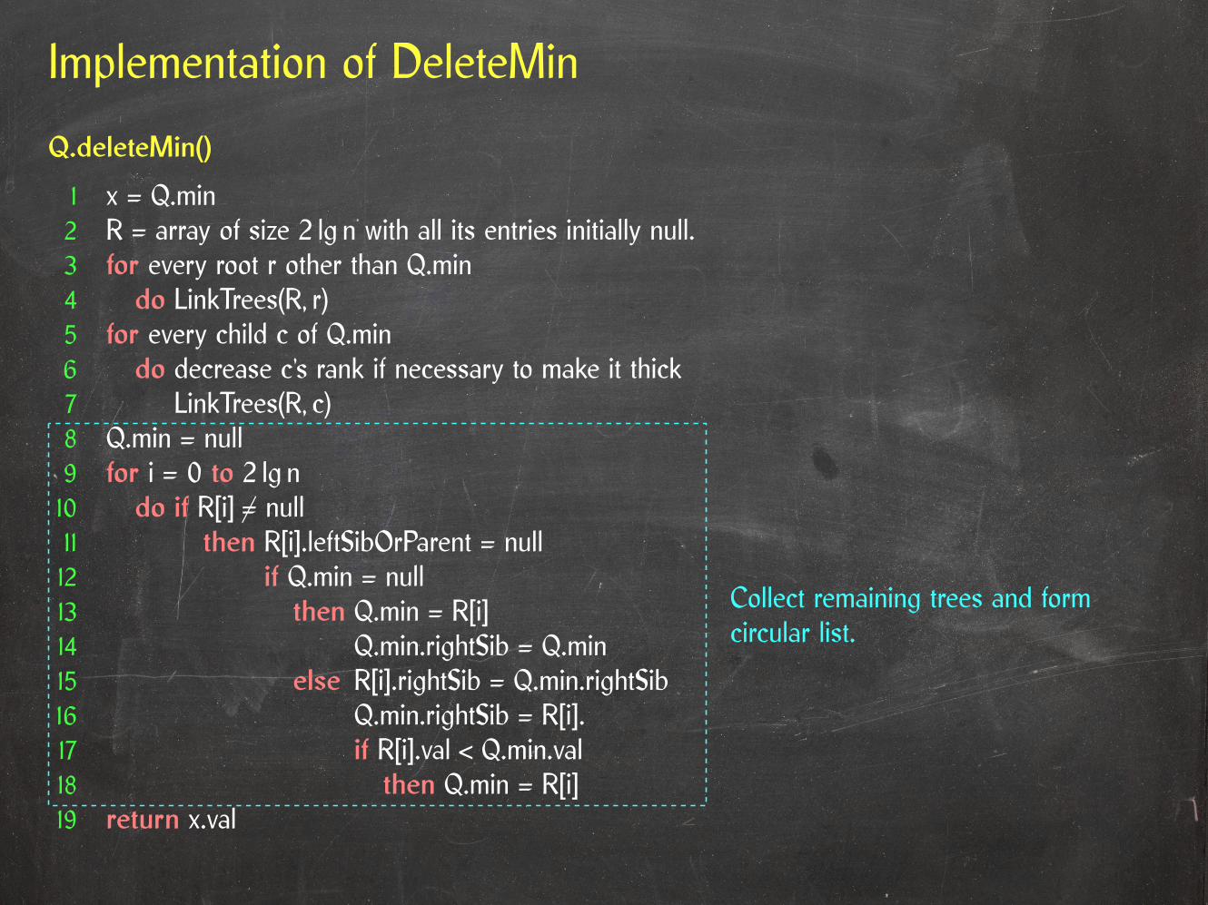
Implementation of DeleteMin
Q.deleteMin()
1 x = Q.min2 R = array of size 2 lg n with all its entries initially null.3 for every root r other than Q.min4 do LinkTrees(R, r)5 for every child c of Q.min6 do decrease c’s rank if necessary to make it thick7 LinkTrees(R, c)8 Q.min = null9 for i = 0 to 2 lg n10 do if R[i] 6= null11 then R[i].leftSibOrParent = null12 if Q.min = null13 then Q.min = R[i]14 Q.min.rightSib = Q.min15 else R[i].rightSib = Q.min.rightSib16 Q.min.rightSib = R[i].17 if R[i].val < Q.min.val18 then Q.min = R[i]19 return x.val
Collect remaining trees and formcircular list.

DecreaseKey
min
x
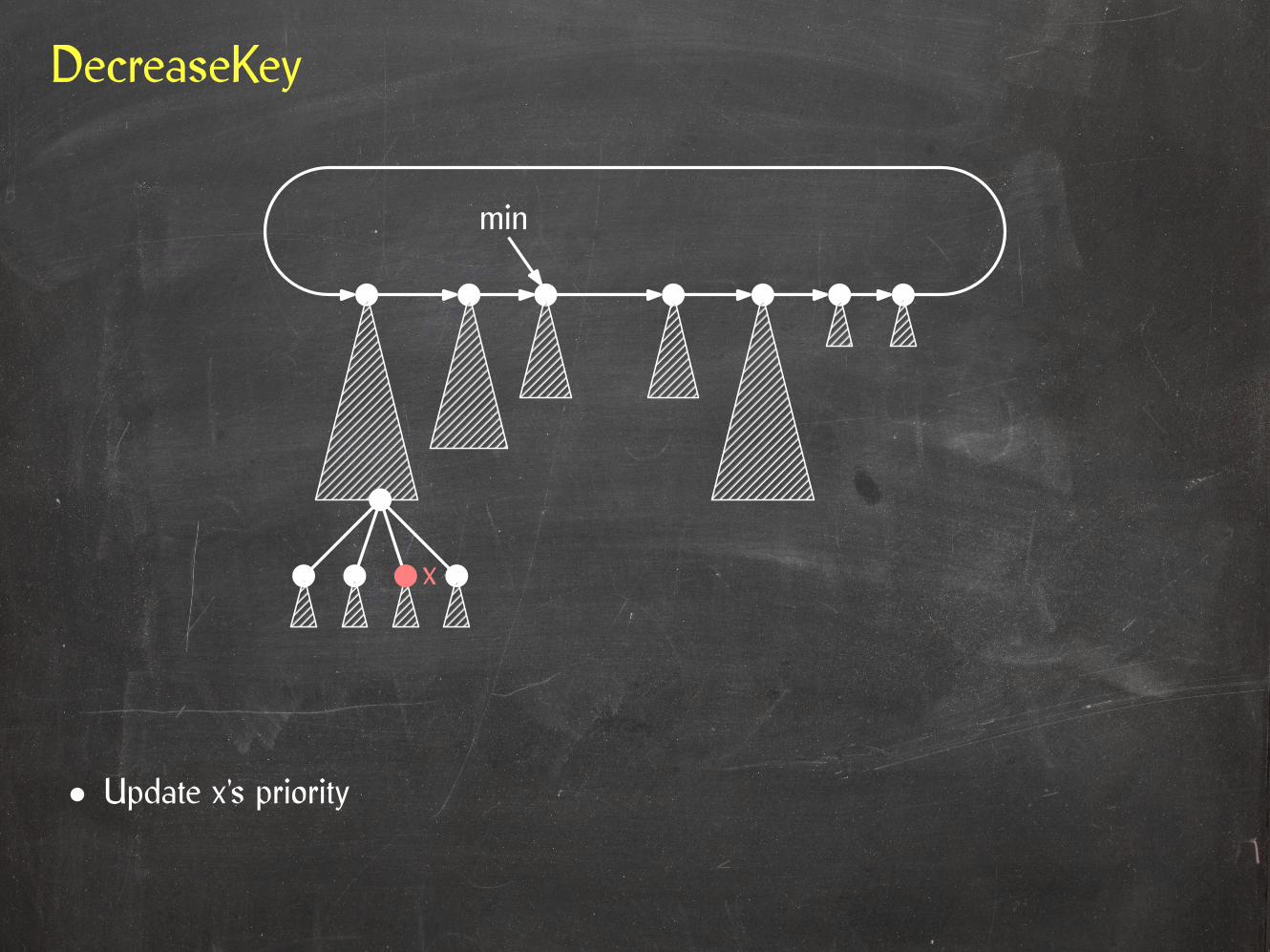
DecreaseKey
• Update x’s priority
min
x
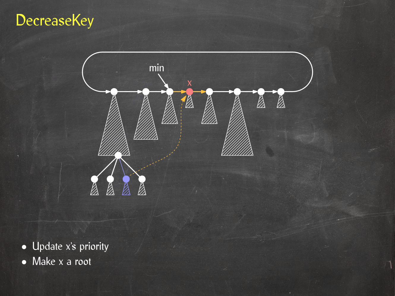
DecreaseKey
• Make x a root• Update x’s priority
minx

DecreaseKey
• Make x a root• Update x’s priority
xmin

DecreaseKey
• Make x a root• Update x’s priority
xmin
Sibling violation at y:
y.rank > 0 and y has no right sibling ory.rightSib.rank < y.rank – 1.

DecreaseKey
• Make x a root• Update x’s priority
xmin
Sibling violation at y:
y.rank > 0 and y has no right sibling ory.rightSib.rank < y.rank – 1.
Parent violation at y:
y.rank > 1 and y has no children ory.child.rank < y.rank – 2.

DecreaseKey
• Fix parent/sibling violations• Make x a root• Update x’s priority
xmin
Sibling violation at y:
y.rank > 0 and y has no right sibling ory.rightSib.rank < y.rank – 1.
Parent violation at y:
y.rank > 1 and y has no children ory.child.rank < y.rank – 2.
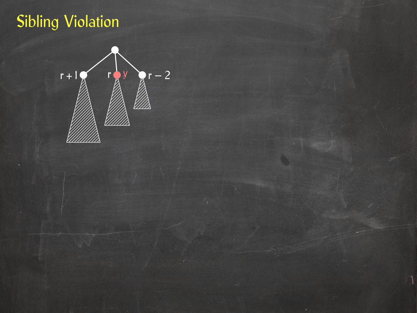
Sibling Violation
r + 1 r r – 2y

Sibling Violation
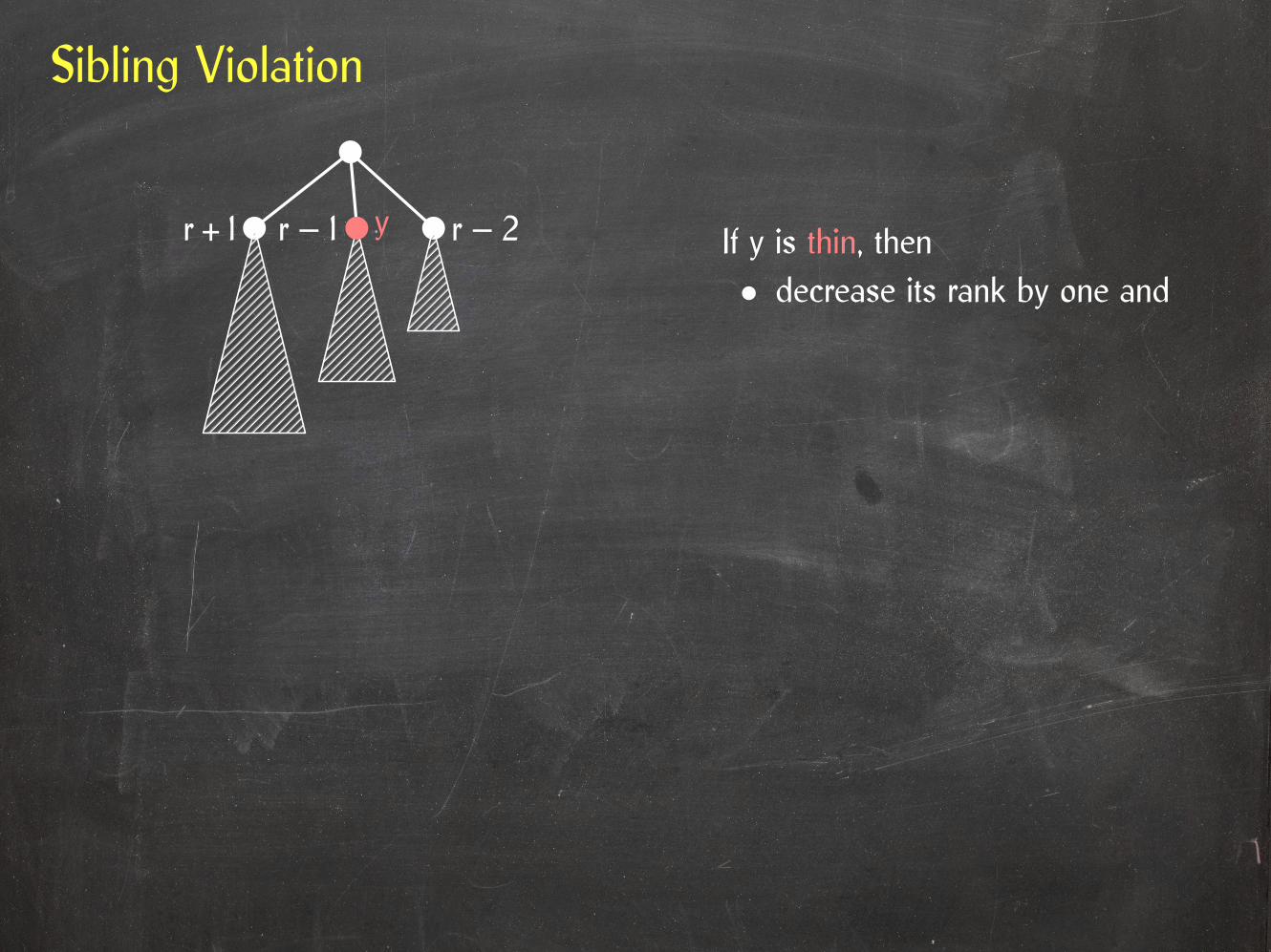
If y is thin, thenr + 1 r r – 2y
Sibling Violation
If y is thin, then• decrease its rank by one and
r + 1 r – 2yr – 1
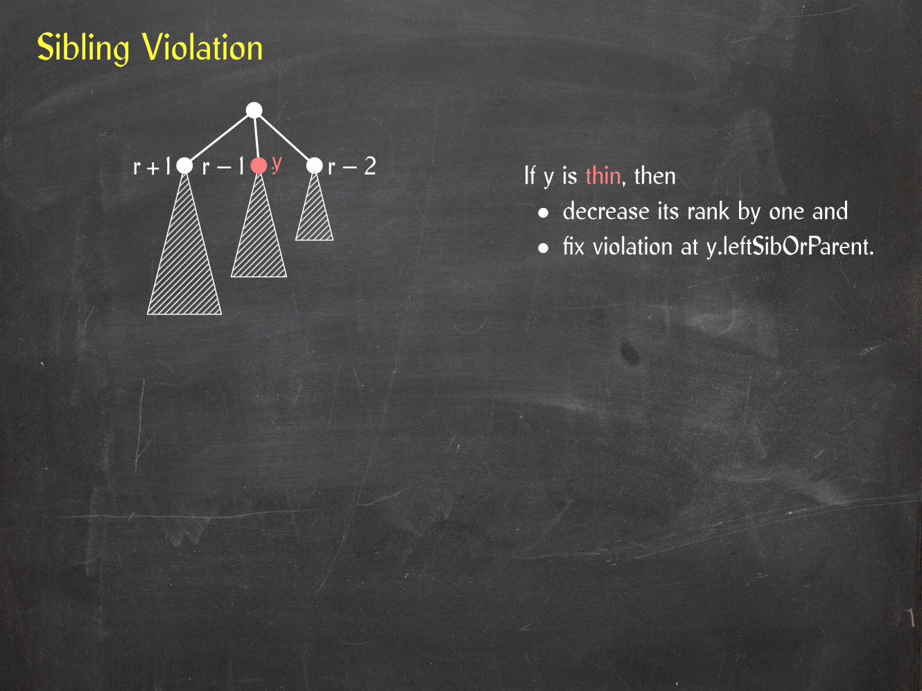
Sibling Violation
If y is thin, then• decrease its rank by one and• fix violation at y.leftSibOrParent.
r + 1 r – 2yr – 1

Sibling Violation
If y is thick, then
If y is thin, then• decrease its rank by one and• fix violation at y.leftSibOrParent.
r + 1 r – 2yr – 1
r – 1 r – 2
r r – 2y

Sibling Violation
r – 1
If y is thin, then• decrease its rank by one and• fix violation at y.leftSibOrParent.
If y is thick, then make y.childy’s right sibling.
r + 1 r – 2yr – 1
r – 2
r r – 1 r – 2y

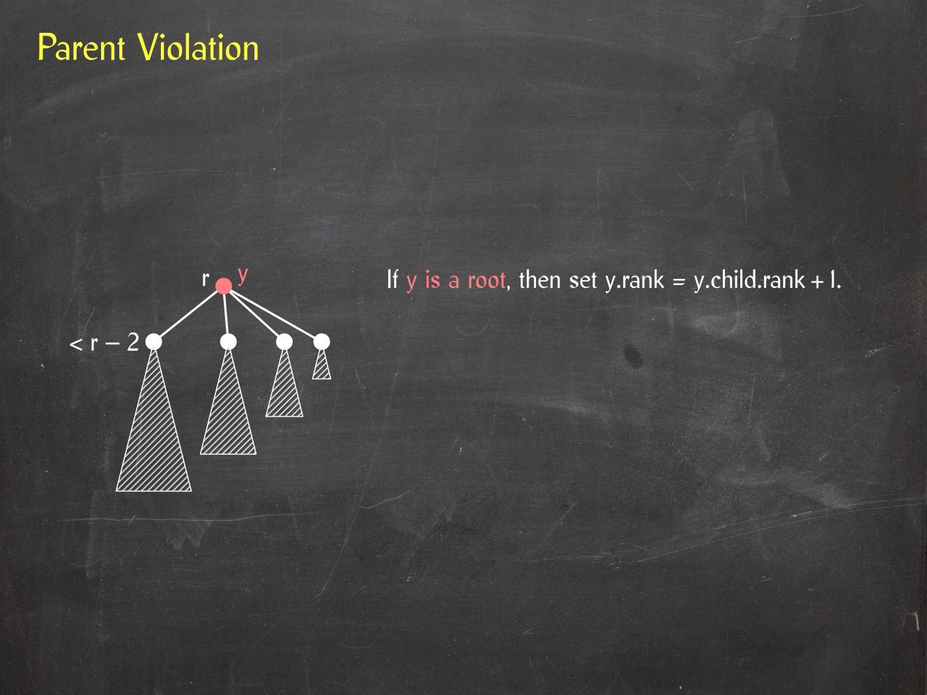
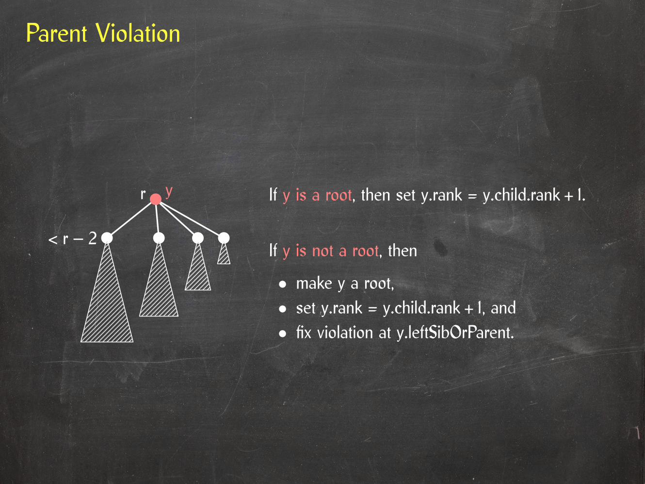
Parent Violation
y
< r – 2
r
Parent Violation
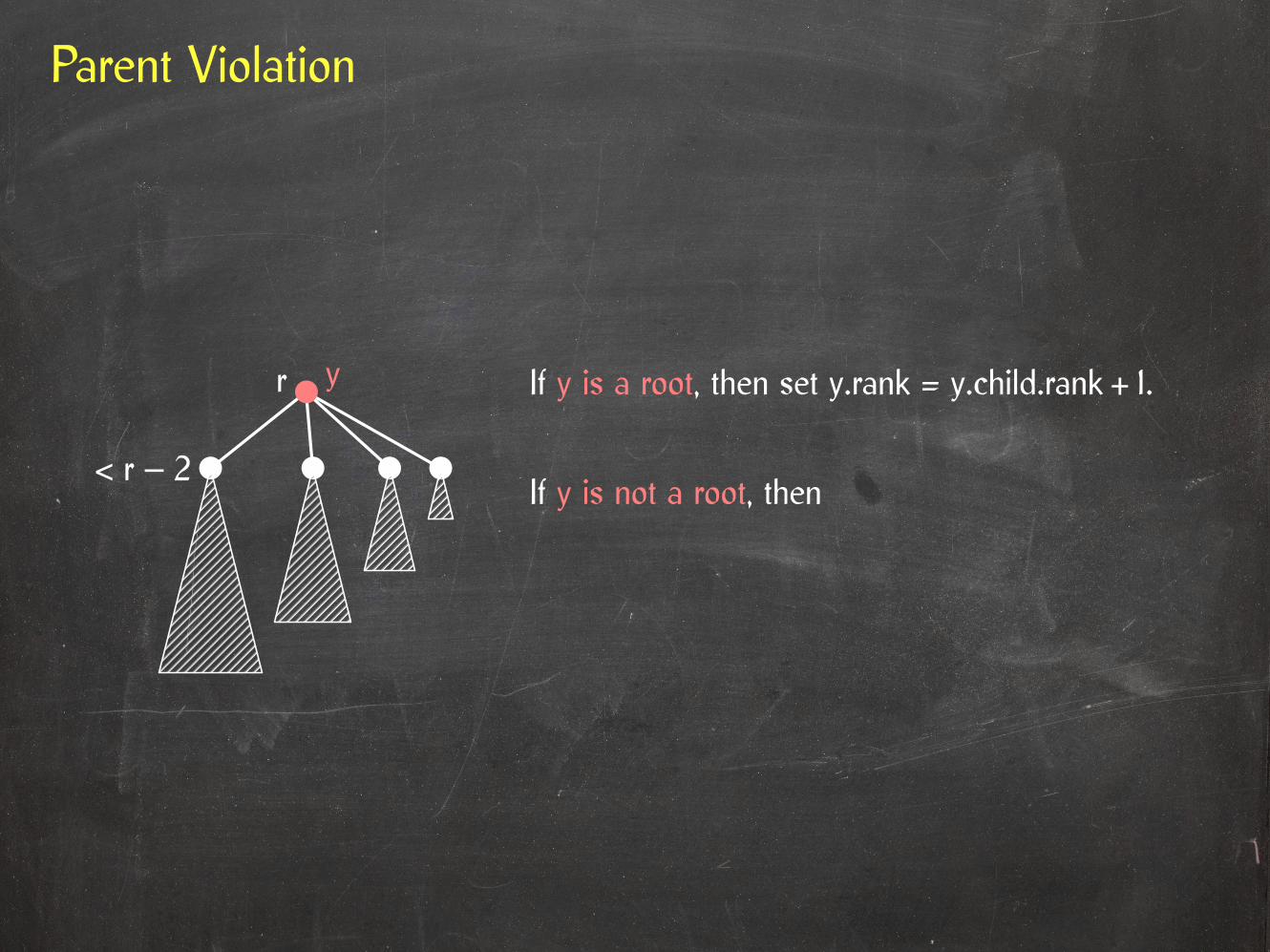
If y is a root, then set y.rank = y.child.rank + 1.y
< r – 2
r
Parent Violation
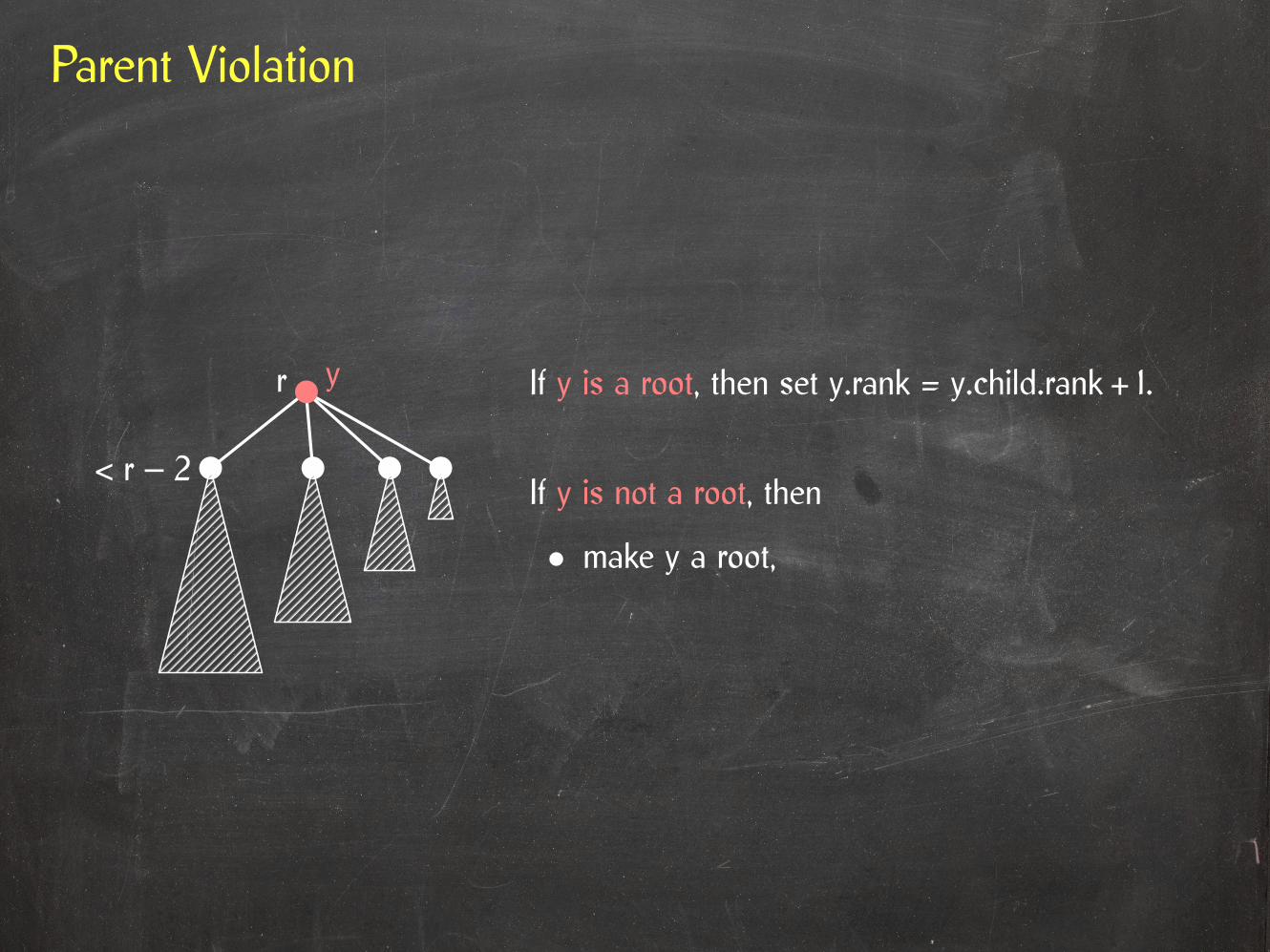
If y is a root, then set y.rank = y.child.rank + 1.
If y is not a root, then
y
< r – 2
r
Parent Violation
If y is a root, then set y.rank = y.child.rank + 1.
• make y a root,
If y is not a root, then
y
< r – 2
r
Parent Violation
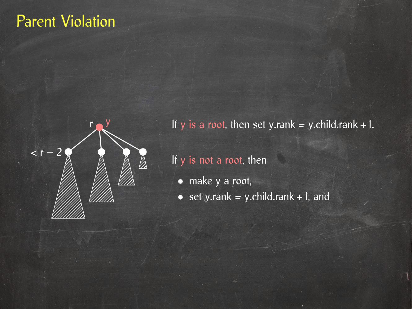
If y is a root, then set y.rank = y.child.rank + 1.
• set y.rank = y.child.rank + 1, and• make y a root,
If y is not a root, then
y
< r – 2
r
Parent Violation
If y is a root, then set y.rank = y.child.rank + 1.
• fix violation at y.leftSibOrParent.• set y.rank = y.child.rank + 1, and• make y a root,
If y is not a root, then
y
< r – 2
r

Amortized Analysis
For a sequence of operations on a data structure, the total worst-case cost of theseoperations is bounded by the sum of the worst-case costs of these operations.

Amortized Analysis
For a sequence of operations on a data structure, the total worst-case cost of theseoperations is bounded by the sum of the worst-case costs of these operations.
We’ve already seen an example where this bound isn’t tight:
• A single Union operation on a union-find data structure can take linear time, but• The total cost of n Union operations is in O(n lg n).
This means: If there’s an expensive operation, there must have been many cheapoperations that can “pay” for this high cost.
Amortized analysis formalizes this idea:
Let o1, o2, . . . , om be a sequence of operations.
Let c1, c2, . . . , cm be their costs.
Now define amortized costs c1, c2, . . . , cm.
These costs are completely fictitious but must satisfy an important condition to beuseful:
m∑i=1
ci ≤m∑i=1
ci

Techniques for Proving Amortized Bounds
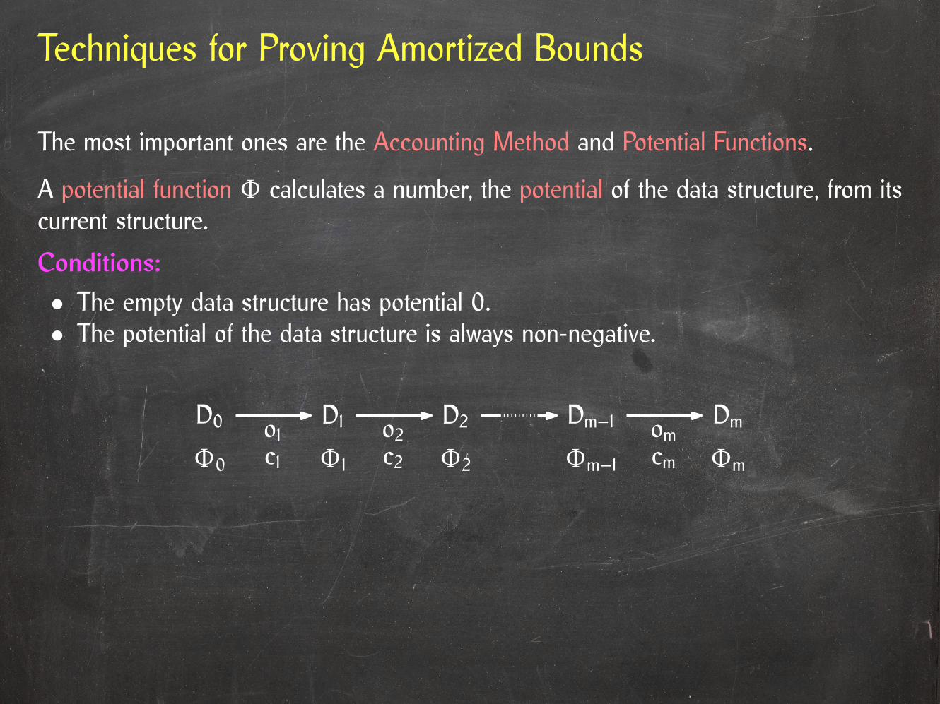
The most important ones are the Accounting Method and Potential Functions.

Techniques for Proving Amortized Bounds
The most important ones are the Accounting Method and Potential Functions.
A potential function Φ calculates a number, the potential of the data structure, from itscurrent structure.
Techniques for Proving Amortized Bounds
The most important ones are the Accounting Method and Potential Functions.
A potential function Φ calculates a number, the potential of the data structure, from itscurrent structure.
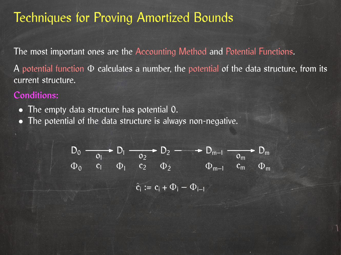
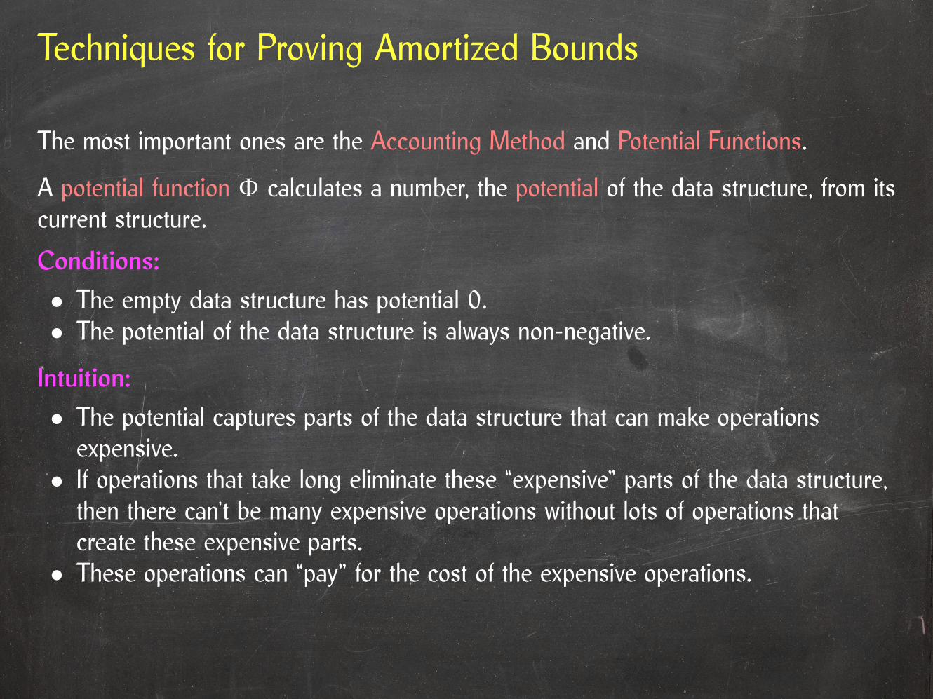
Conditions:
• The empty data structure has potential 0.• The potential of the data structure is always non-negative.
Techniques for Proving Amortized Bounds
The most important ones are the Accounting Method and Potential Functions.
A potential function Φ calculates a number, the potential of the data structure, from itscurrent structure.
Conditions:
• The empty data structure has potential 0.• The potential of the data structure is always non-negative.
D0 D1 D2 Dmo1 o2 omDm–1

Techniques for Proving Amortized Bounds
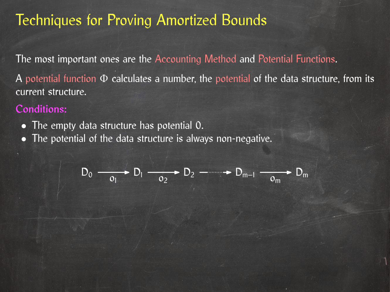
The most important ones are the Accounting Method and Potential Functions.
A potential function Φ calculates a number, the potential of the data structure, from itscurrent structure.
Conditions:
• The empty data structure has potential 0.• The potential of the data structure is always non-negative.
D0 D1 D2 Dmo1 o2 omDm–1
c1 c2 cm
Techniques for Proving Amortized Bounds
The most important ones are the Accounting Method and Potential Functions.
A potential function Φ calculates a number, the potential of the data structure, from itscurrent structure.
Conditions:
• The empty data structure has potential 0.• The potential of the data structure is always non-negative.
D0 D1 D2 Dmo1 o2 omDm–1
Φ0 Φ1 Φ2 Φm–1 Φmc1 c2 cm
Techniques for Proving Amortized Bounds
The most important ones are the Accounting Method and Potential Functions.
A potential function Φ calculates a number, the potential of the data structure, from itscurrent structure.
Conditions:
• The empty data structure has potential 0.• The potential of the data structure is always non-negative.
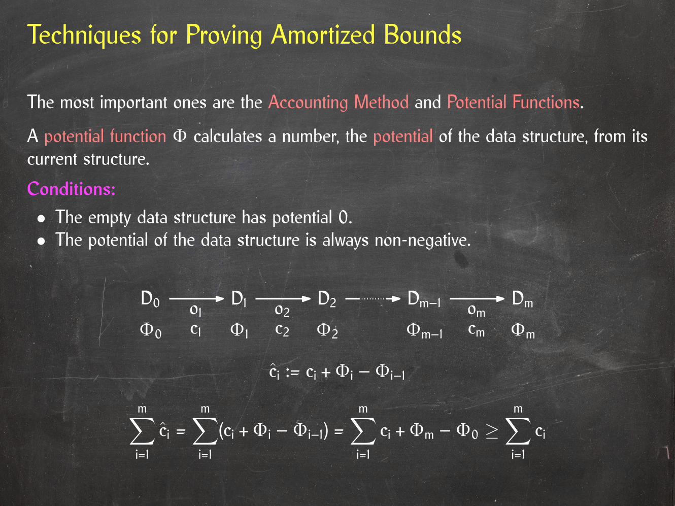
ci := ci +Φi –Φi–1
D0 D1 D2 Dmo1 o2 omDm–1
Φ0 Φ1 Φ2 Φm–1 Φmc1 c2 cm
Techniques for Proving Amortized Bounds
The most important ones are the Accounting Method and Potential Functions.
A potential function Φ calculates a number, the potential of the data structure, from itscurrent structure.
Conditions:
• The empty data structure has potential 0.• The potential of the data structure is always non-negative.
ci := ci +Φi –Φi–1
m∑i=1
ci =m∑i=1
(ci +Φi –Φi–1) =m∑i=1
ci +Φm –Φ0 ≥m∑i=1
ci
D0 D1 D2 Dmo1 o2 omDm–1
Φ0 Φ1 Φ2 Φm–1 Φmc1 c2 cm
Techniques for Proving Amortized Bounds
The most important ones are the Accounting Method and Potential Functions.
A potential function Φ calculates a number, the potential of the data structure, from itscurrent structure.
Conditions:
• The empty data structure has potential 0.• The potential of the data structure is always non-negative.
Intuition:
• The potential captures parts of the data structure that can make operationsexpensive.• If operations that take long eliminate these “expensive” parts of the data structure,then there can’t be many expensive operations without lots of operations thatcreate these expensive parts.• These operations can “pay” for the cost of the expensive operations.

Amortized Analysis: Stack with MultiPop Operation
Operations:
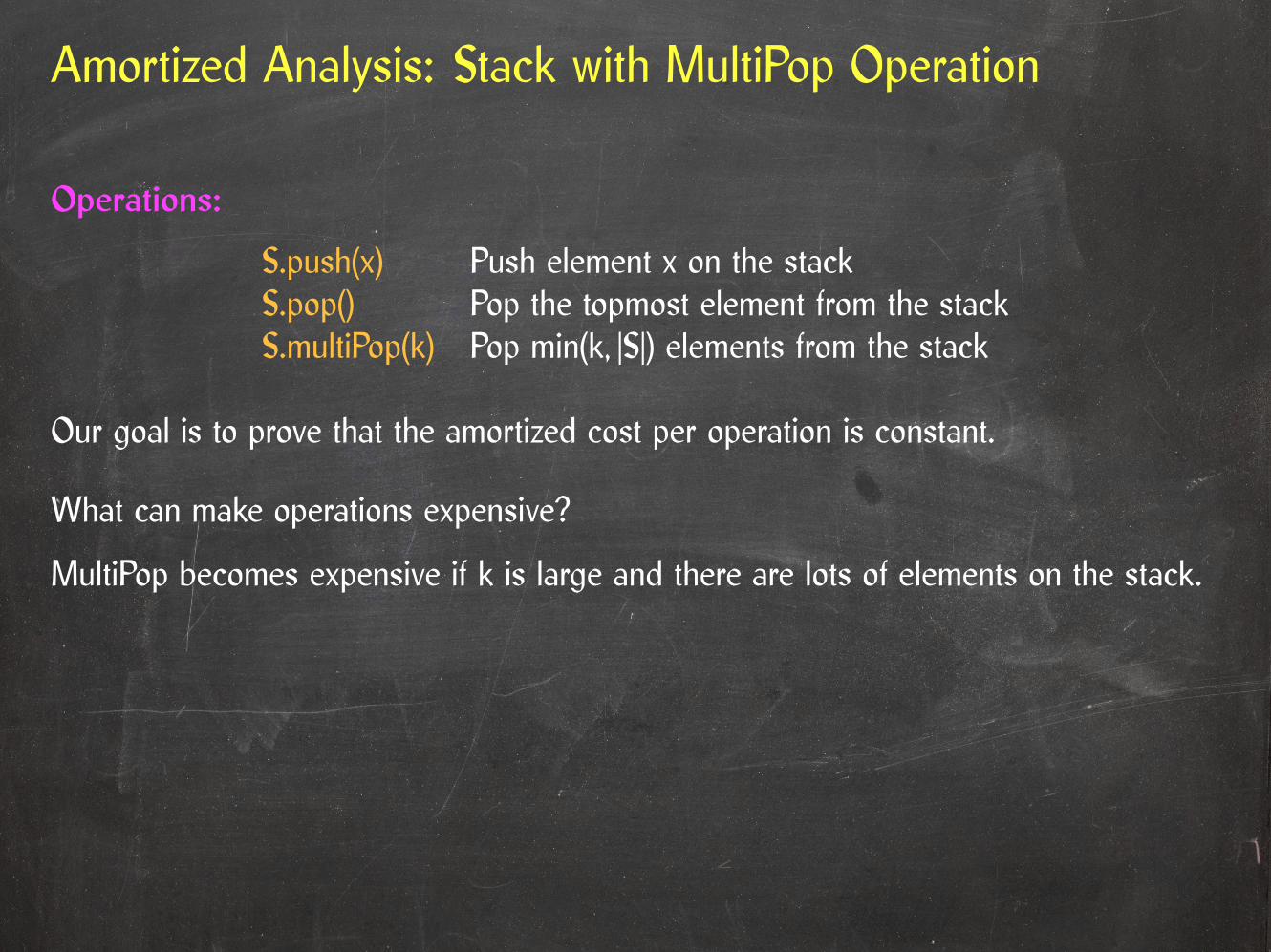
S.push(x) Push element x on the stackS.pop() Pop the topmost element from the stackS.multiPop(k) Pop min(k, |S|) elements from the stack

Amortized Analysis: Stack with MultiPop Operation
Operations:
S.push(x) Push element x on the stackS.pop() Pop the topmost element from the stackS.multiPop(k) Pop min(k, |S|) elements from the stack
Our goal is to prove that the amortized cost per operation is constant.

Amortized Analysis: Stack with MultiPop Operation
Operations:
S.push(x) Push element x on the stackS.pop() Pop the topmost element from the stackS.multiPop(k) Pop min(k, |S|) elements from the stack
Our goal is to prove that the amortized cost per operation is constant.
What can make operations expensive?
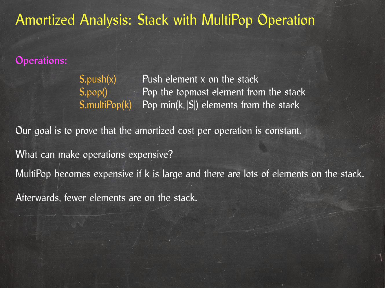
MultiPop becomes expensive if k is large and there are lots of elements on the stack.
Amortized Analysis: Stack with MultiPop Operation
Operations:
S.push(x) Push element x on the stackS.pop() Pop the topmost element from the stackS.multiPop(k) Pop min(k, |S|) elements from the stack
Our goal is to prove that the amortized cost per operation is constant.
What can make operations expensive?
MultiPop becomes expensive if k is large and there are lots of elements on the stack.
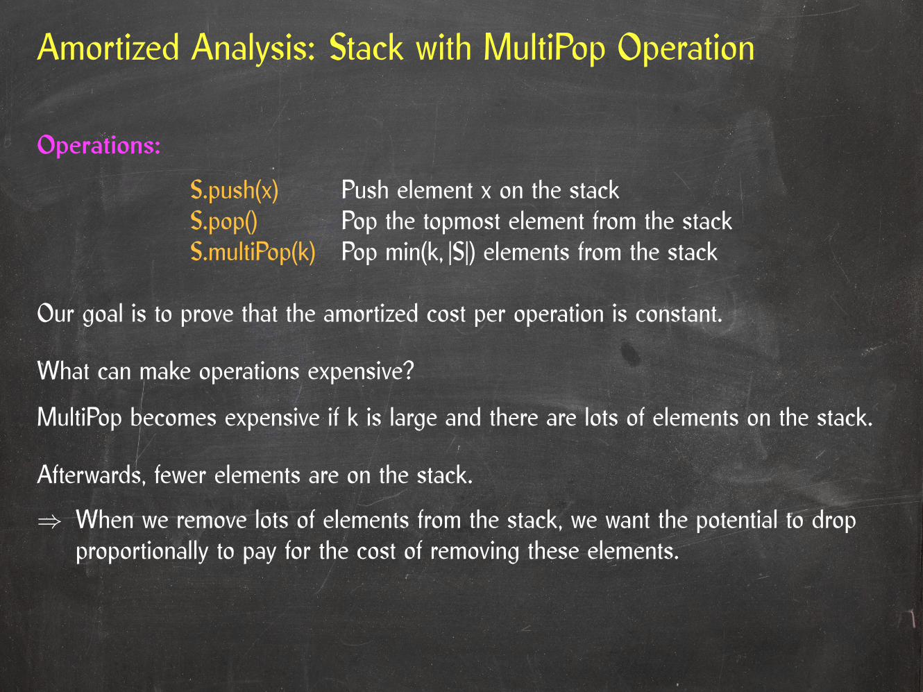
Afterwards, fewer elements are on the stack.
Amortized Analysis: Stack with MultiPop Operation
Operations:
S.push(x) Push element x on the stackS.pop() Pop the topmost element from the stackS.multiPop(k) Pop min(k, |S|) elements from the stack
Our goal is to prove that the amortized cost per operation is constant.
What can make operations expensive?
MultiPop becomes expensive if k is large and there are lots of elements on the stack.
Afterwards, fewer elements are on the stack.
⇒ When we remove lots of elements from the stack, we want the potential to dropproportionally to pay for the cost of removing these elements.

Amortized Analysis: Stack with MultiPop Operation
Operations:
S.push(x) Push element x on the stackS.pop() Pop the topmost element from the stackS.multiPop(k) Pop min(k, |S|) elements from the stack
Our goal is to prove that the amortized cost per operation is constant.
Φ = |S|
What can make operations expensive?
MultiPop becomes expensive if k is large and there are lots of elements on the stack.
Afterwards, fewer elements are on the stack.
⇒ When we remove lots of elements from the stack, we want the potential to dropproportionally to pay for the cost of removing these elements.

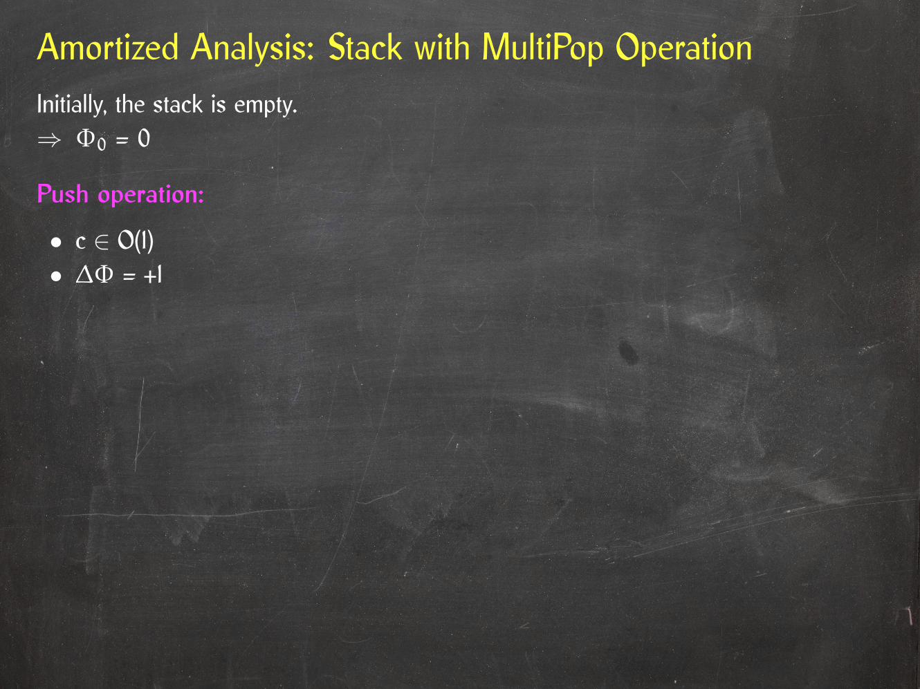
Amortized Analysis: Stack with MultiPop OperationInitially, the stack is empty.⇒ Φ0 = 0
Amortized Analysis: Stack with MultiPop OperationInitially, the stack is empty.⇒ Φ0 = 0
Push operation:

Amortized Analysis: Stack with MultiPop OperationInitially, the stack is empty.⇒ Φ0 = 0
Push operation:
• c ∈ O(1)
Amortized Analysis: Stack with MultiPop OperationInitially, the stack is empty.⇒ Φ0 = 0
Push operation:
• c ∈ O(1)• ∆Φ = +1

Amortized Analysis: Stack with MultiPop OperationInitially, the stack is empty.⇒ Φ0 = 0
Push operation:
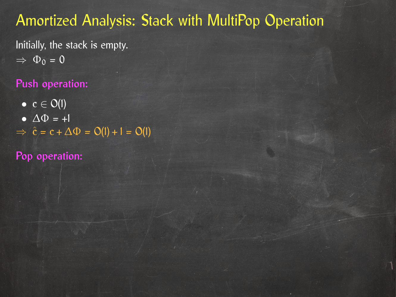
• c ∈ O(1)• ∆Φ = +1⇒ c = c + ∆Φ = O(1) + 1 = O(1)
Amortized Analysis: Stack with MultiPop OperationInitially, the stack is empty.⇒ Φ0 = 0
Pop operation:
Push operation:
• c ∈ O(1)• ∆Φ = +1⇒ c = c + ∆Φ = O(1) + 1 = O(1)

Amortized Analysis: Stack with MultiPop OperationInitially, the stack is empty.⇒ Φ0 = 0
Pop operation:
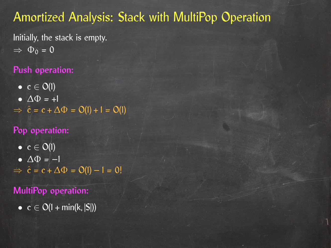
• c ∈ O(1)
Push operation:
• c ∈ O(1)• ∆Φ = +1⇒ c = c + ∆Φ = O(1) + 1 = O(1)

Amortized Analysis: Stack with MultiPop OperationInitially, the stack is empty.⇒ Φ0 = 0
Pop operation:
• c ∈ O(1)• ∆Φ = –1
Push operation:
• c ∈ O(1)• ∆Φ = +1⇒ c = c + ∆Φ = O(1) + 1 = O(1)

Amortized Analysis: Stack with MultiPop OperationInitially, the stack is empty.⇒ Φ0 = 0
Pop operation:
• c ∈ O(1)• ∆Φ = –1⇒ c = c + ∆Φ = O(1) – 1 = 0!
Push operation:
• c ∈ O(1)• ∆Φ = +1⇒ c = c + ∆Φ = O(1) + 1 = O(1)

Amortized Analysis: Stack with MultiPop OperationInitially, the stack is empty.⇒ Φ0 = 0
MultiPop operation:
Pop operation:
• c ∈ O(1)• ∆Φ = –1⇒ c = c + ∆Φ = O(1) – 1 = 0!
Push operation:
• c ∈ O(1)• ∆Φ = +1⇒ c = c + ∆Φ = O(1) + 1 = O(1)
Amortized Analysis: Stack with MultiPop OperationInitially, the stack is empty.⇒ Φ0 = 0
MultiPop operation:
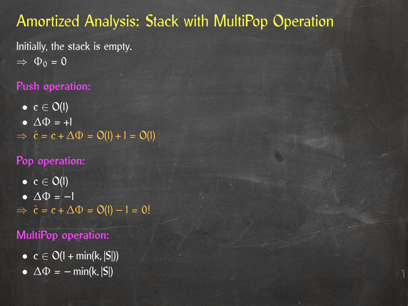
• c ∈ O(1 + min(k, |S|))
Pop operation:
• c ∈ O(1)• ∆Φ = –1⇒ c = c + ∆Φ = O(1) – 1 = 0!
Push operation:
• c ∈ O(1)• ∆Φ = +1⇒ c = c + ∆Φ = O(1) + 1 = O(1)
Amortized Analysis: Stack with MultiPop OperationInitially, the stack is empty.⇒ Φ0 = 0
MultiPop operation:
• c ∈ O(1 + min(k, |S|))• ∆Φ = –min(k, |S|)
Pop operation:
• c ∈ O(1)• ∆Φ = –1⇒ c = c + ∆Φ = O(1) – 1 = 0!
Push operation:
• c ∈ O(1)• ∆Φ = +1⇒ c = c + ∆Φ = O(1) + 1 = O(1)

Amortized Analysis: Stack with MultiPop OperationInitially, the stack is empty.⇒ Φ0 = 0
MultiPop operation:
• c ∈ O(1 + min(k, |S|))• ∆Φ = –min(k, |S|)⇒ c = c + ∆Φ = O(1 + min(k, |S|)) – min(k, |S|) = O(1)
Pop operation:
• c ∈ O(1)• ∆Φ = –1⇒ c = c + ∆Φ = O(1) – 1 = 0!
Push operation:
• c ∈ O(1)• ∆Φ = +1⇒ c = c + ∆Φ = O(1) + 1 = O(1)
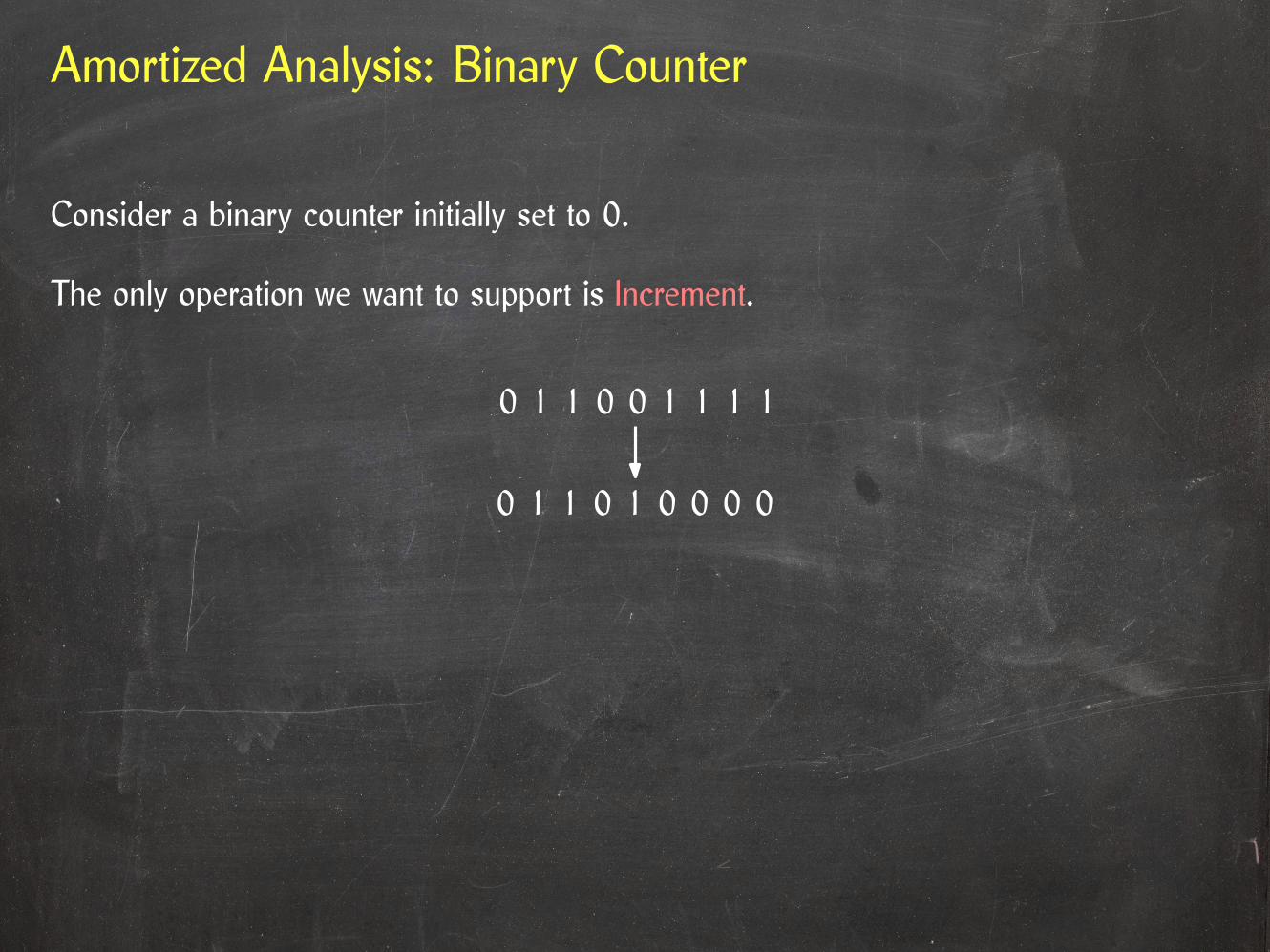
Amortized Analysis: Binary Counter
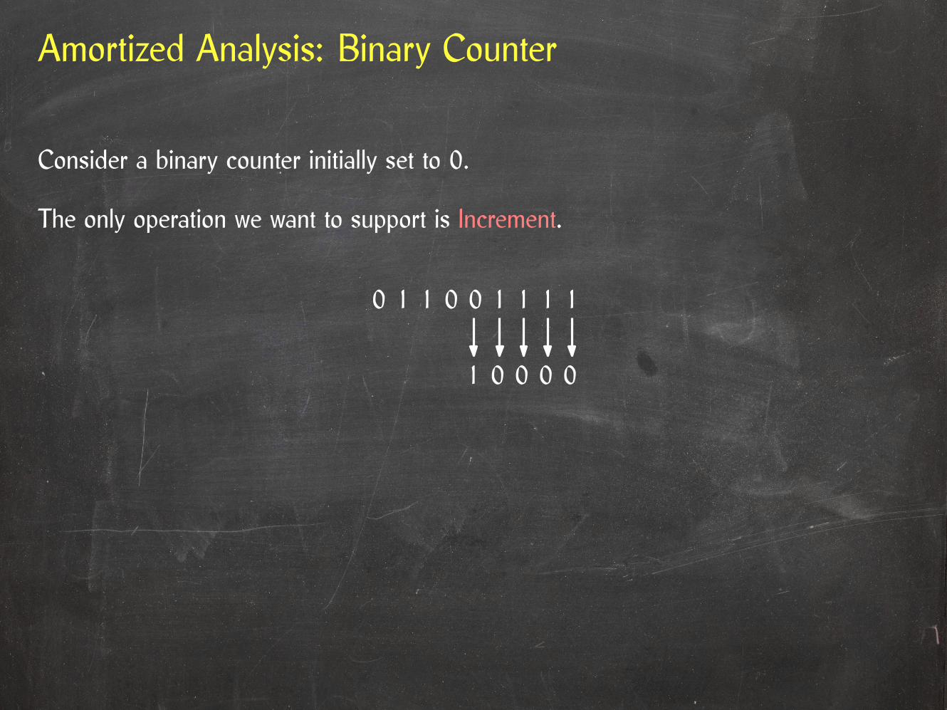
Consider a binary counter initially set to 0.
The only operation we want to support is Increment.
0 101 1 0 1 1 1
0 00 011 0 01

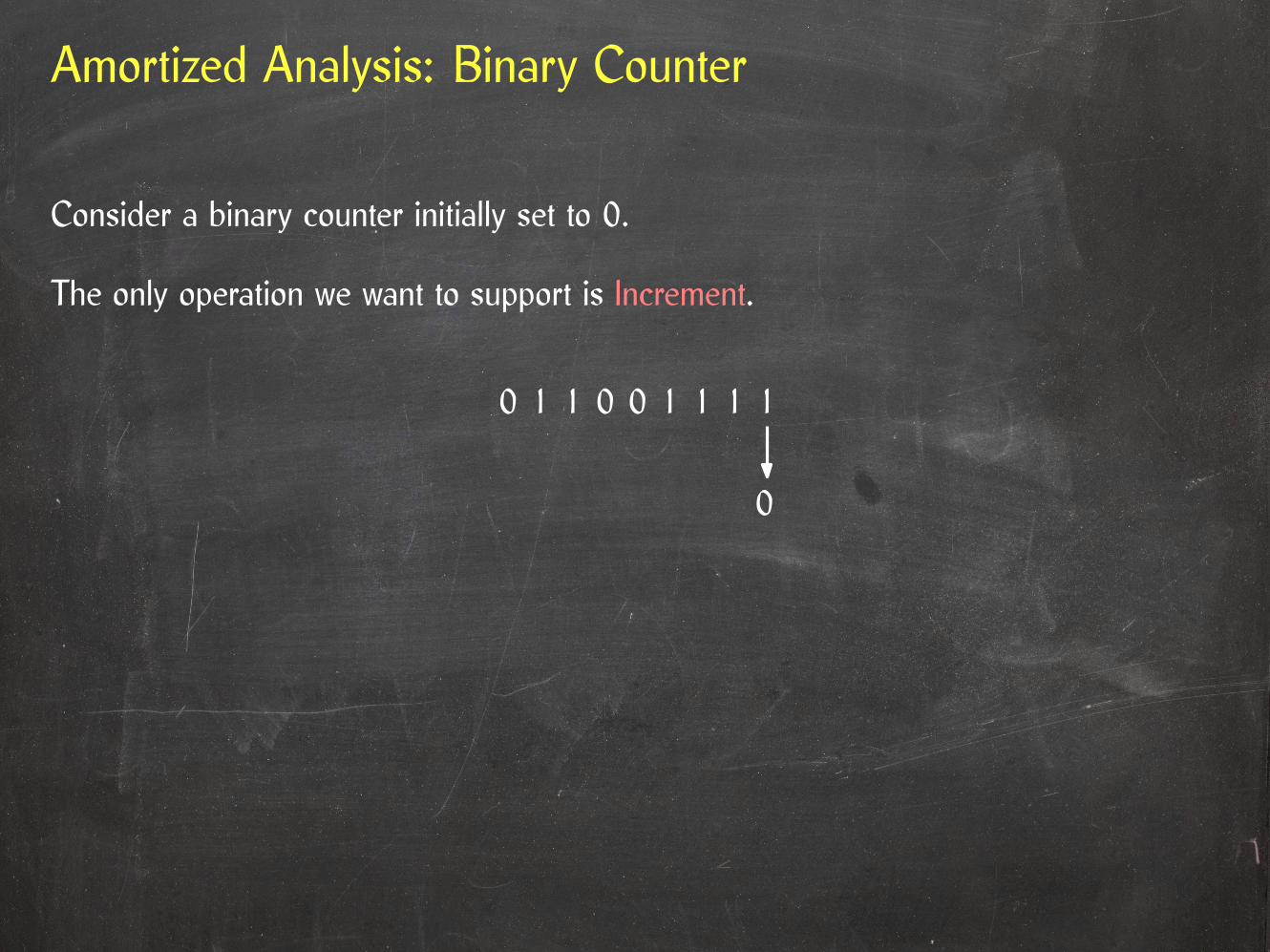
Amortized Analysis: Binary Counter
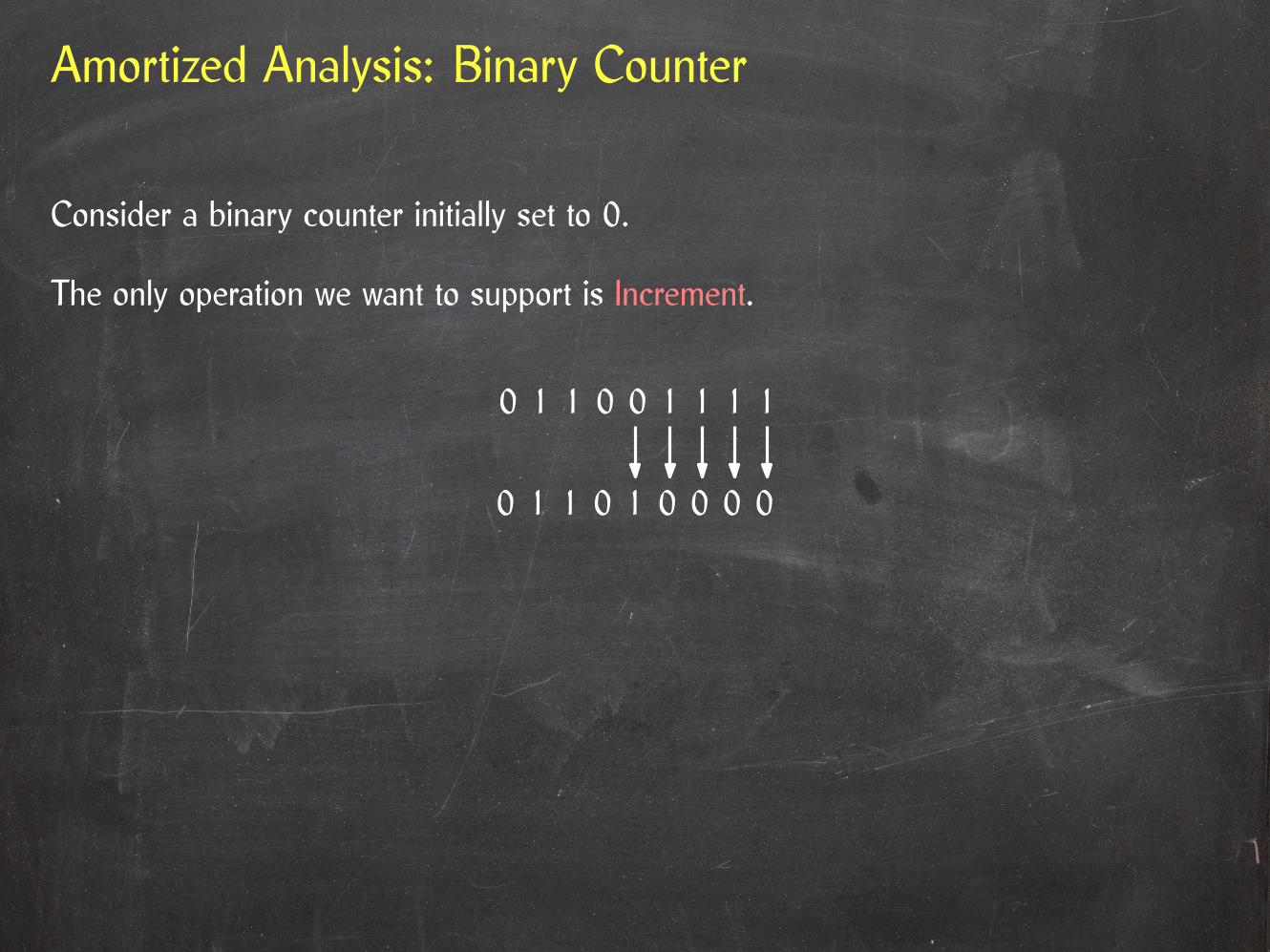
Consider a binary counter initially set to 0.
The only operation we want to support is Increment.
0 101 1 0 1 1 1
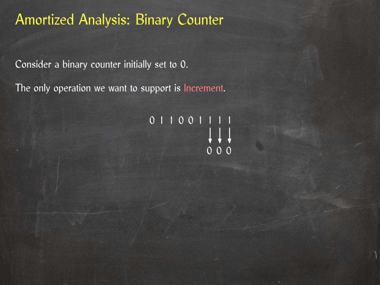
Amortized Analysis: Binary Counter
Consider a binary counter initially set to 0.
The only operation we want to support is Increment.
0 101 1 0 1 1 1
0

Amortized Analysis: Binary Counter
Consider a binary counter initially set to 0.
The only operation we want to support is Increment.
0 101 1 0 1 1 1
0 0
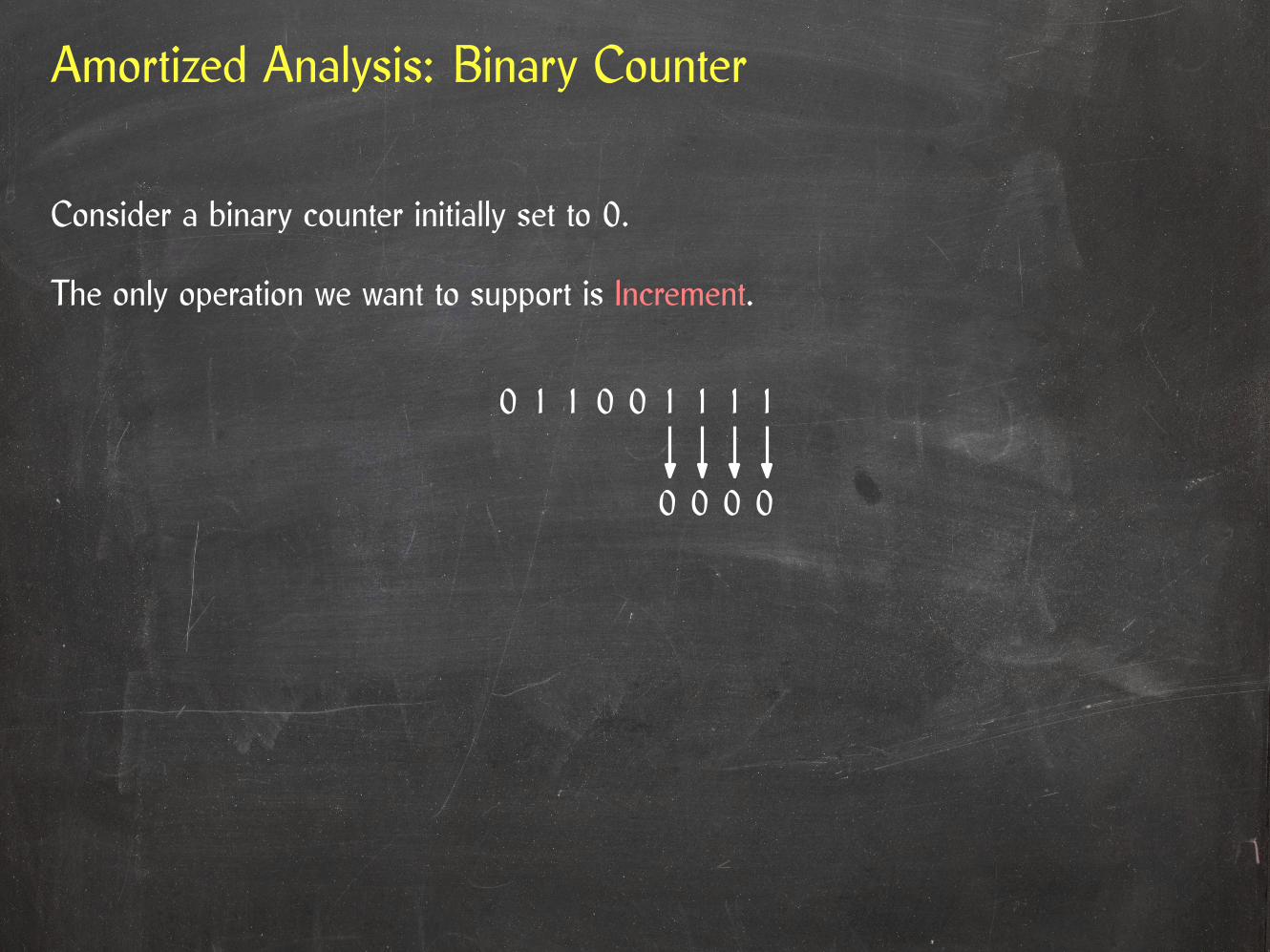
Amortized Analysis: Binary Counter
Consider a binary counter initially set to 0.
The only operation we want to support is Increment.
0 101 1 0 1 1 1
00 0
Amortized Analysis: Binary Counter
Consider a binary counter initially set to 0.
The only operation we want to support is Increment.
0 101 1 0 1 1 1
00 0 0
Amortized Analysis: Binary Counter
Consider a binary counter initially set to 0.
The only operation we want to support is Increment.
0 101 1 0 1 1 1
00 01 0
Amortized Analysis: Binary Counter
Consider a binary counter initially set to 0.
The only operation we want to support is Increment.
0 101 1 0 1 1 1
0 00 011 0 01
Amortized Analysis: Binary Counter
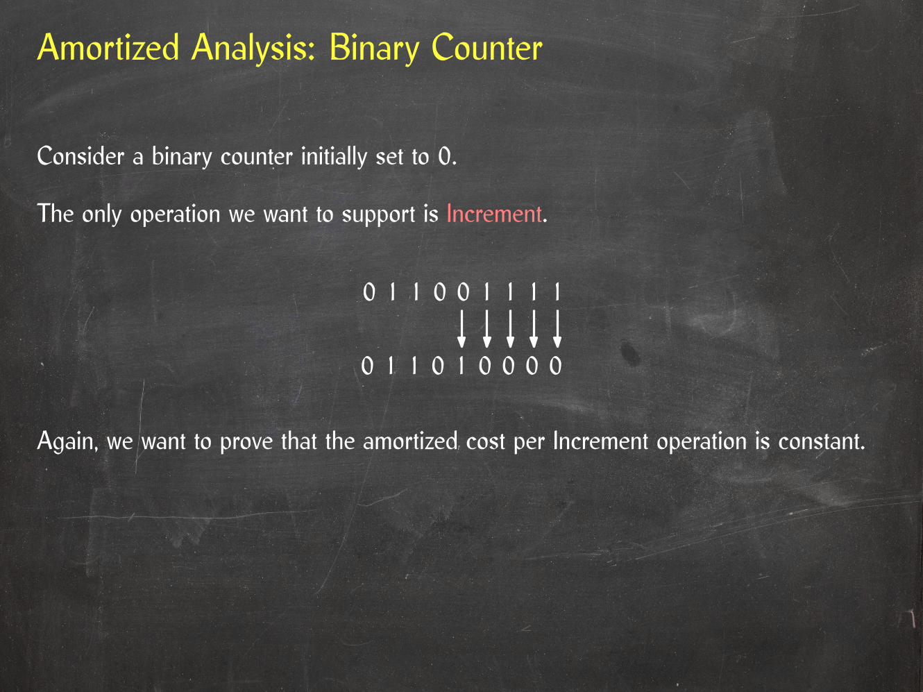
Consider a binary counter initially set to 0.
The only operation we want to support is Increment.
Again, we want to prove that the amortized cost per Increment operation is constant.
0 101 1 0 1 1 1
0 00 011 0 01

Amortized Analysis: Binary Counter
Consider a binary counter initially set to 0.
The only operation we want to support is Increment.
Again, we want to prove that the amortized cost per Increment operation is constant.
What makes increment operations expensive?
0 101 1 0 1 1 1
0 00 011 0 01

Amortized Analysis: Binary Counter
Consider a binary counter initially set to 0.
The only operation we want to support is Increment.
Again, we want to prove that the amortized cost per Increment operation is constant.
What makes increment operations expensive?
Lots of 1s that need to be flipped into 0s.
0 101 1 0 1 1 1
0 00 011 0 01

Amortized Analysis: Binary Counter
Consider a binary counter initially set to 0.
The only operation we want to support is Increment.
Again, we want to prove that the amortized cost per Increment operation is constant.
Φ = #1s in the current counter value
What makes increment operations expensive?
Lots of 1s that need to be flipped into 0s.
0 101 1 0 1 1 1
0 00 011 0 01
Amortized Analysis: Binary Counter
Initially, all digits are 0.
⇒ Φ0 = 0
Amortized Analysis: Binary Counter
If the rightmost 0 is the kth digit from the right, then an Increment operation takesO(k) time.
Initially, all digits are 0.
⇒ Φ0 = 0
Amortized Analysis: Binary Counter
If the rightmost 0 is the kth digit from the right, then an Increment operation takesO(k) time.
The operation turns the kth digit into a 1 and turns the k – 1 1s to its right into 0s.
Initially, all digits are 0.
⇒ Φ0 = 0
Amortized Analysis: Binary Counter
If the rightmost 0 is the kth digit from the right, then an Increment operation takesO(k) time.
The operation turns the kth digit into a 1 and turns the k – 1 1s to its right into 0s.
⇒ ∆Φ = +1 – (k – 1) = 2 – k
Initially, all digits are 0.
⇒ Φ0 = 0

Amortized Analysis: Binary Counter
If the rightmost 0 is the kth digit from the right, then an Increment operation takesO(k) time.
The operation turns the kth digit into a 1 and turns the k – 1 1s to its right into 0s.
⇒ ∆Φ = +1 – (k – 1) = 2 – k
⇒ c = c + ∆Φ = O(k) + 2 – k = O(1)
Initially, all digits are 0.
⇒ Φ0 = 0
A Potential Function for Thin Heap
What makes Thin Heap operations expensive?
A Potential Function for Thin Heap
What makes Thin Heap operations expensive?
• DeleteMin: Many roots.
A Potential Function for Thin Heap
What makes Thin Heap operations expensive?
• DeleteMin: Many roots.• DecreaseKey: Many thin nodes.

A Potential Function for Thin Heap
What makes Thin Heap operations expensive?
• DeleteMin: Many roots.• DecreaseKey: Many thin nodes.
⇒ The potential function should count roots and thin nodes.
A Potential Function for Thin Heap
What makes Thin Heap operations expensive?
• DeleteMin: Many roots.• DecreaseKey: Many thin nodes.
⇒ The potential function should count roots and thin nodes.
A DecreaseKey operation may turn many thin nodes into roots. If we want anamortized cost of O(1) for DecreaseKey, this needs to be paid for by a drop in potential.
⇒ Thin nodes should be “more expensive” than roots.
Φ = 2 · number of thin nodes + number of roots
Amortized Cost of Insert, FindMin, and Delete
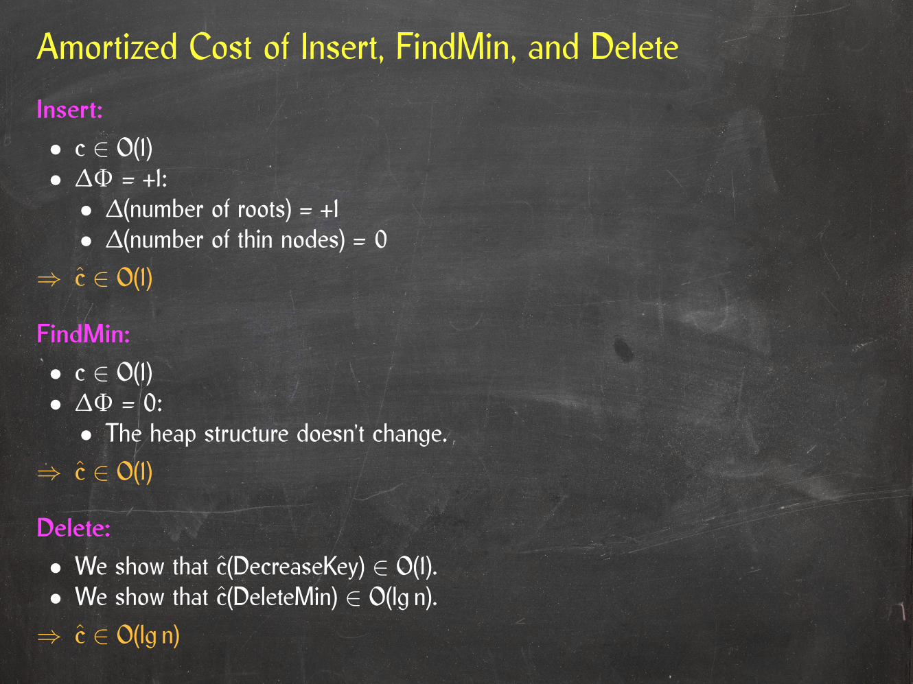
Insert:
• c ∈ O(1)• ∆Φ = +1:• ∆(number of roots) = +1• ∆(number of thin nodes) = 0
⇒ c ∈ O(1)

Amortized Cost of Insert, FindMin, and Delete
Insert:
• c ∈ O(1)• ∆Φ = +1:• ∆(number of roots) = +1• ∆(number of thin nodes) = 0
⇒ c ∈ O(1)
FindMin:
• c ∈ O(1)• ∆Φ = 0:• The heap structure doesn’t change.
⇒ c ∈ O(1)
Amortized Cost of Insert, FindMin, and Delete
Insert:
• c ∈ O(1)• ∆Φ = +1:• ∆(number of roots) = +1• ∆(number of thin nodes) = 0
⇒ c ∈ O(1)
FindMin:
• c ∈ O(1)• ∆Φ = 0:• The heap structure doesn’t change.
⇒ c ∈ O(1)
Delete:
• We show that c(DecreaseKey) ∈ O(1).• We show that c(DeleteMin) ∈ O(lg n).
⇒ c ∈ O(lg n)
Amortized Cost of DeleteMin
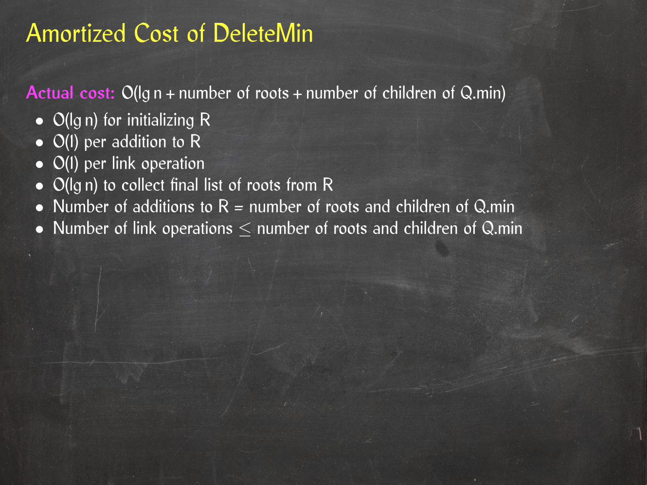
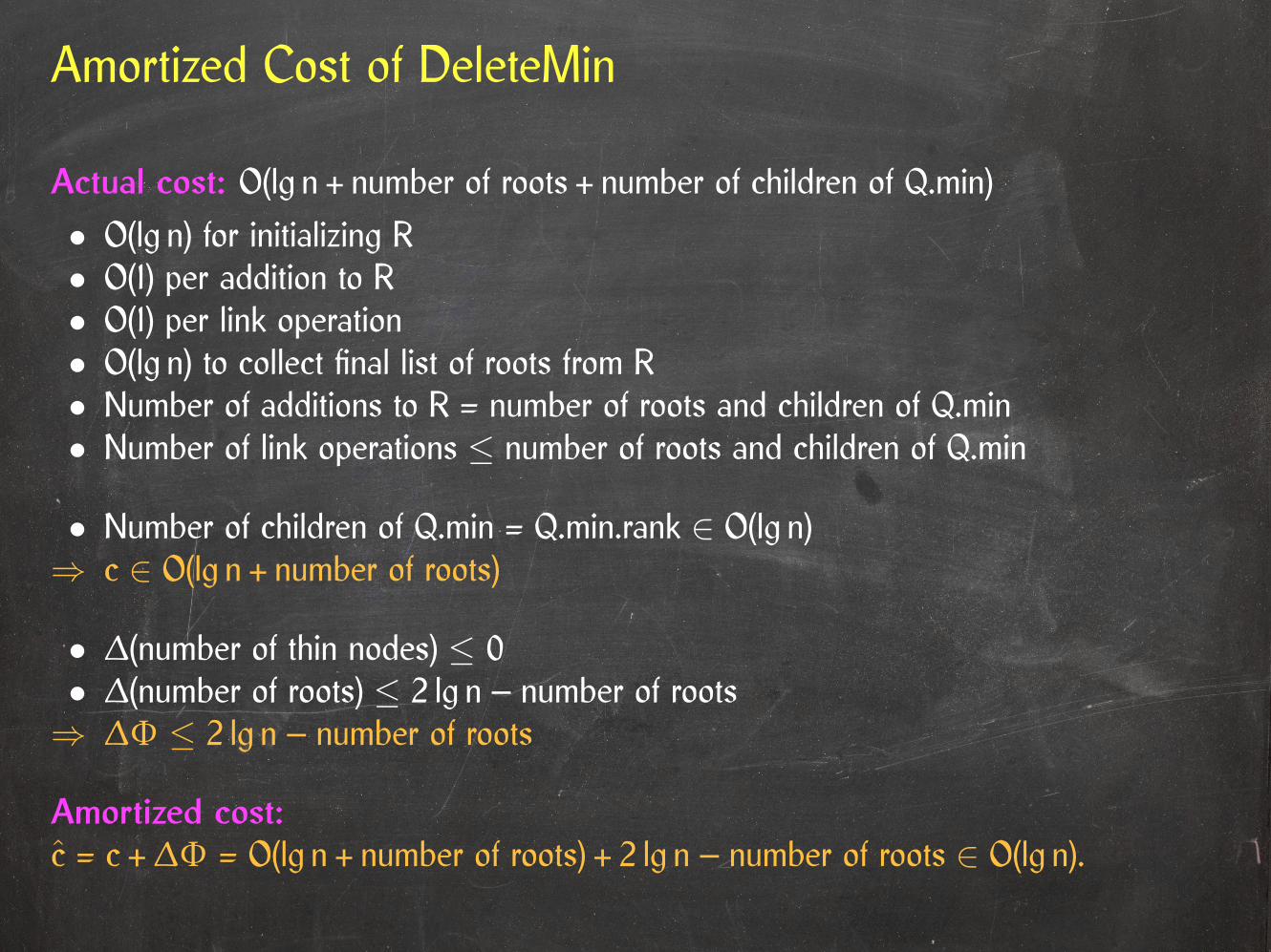
Actual cost: O(lg n + number of roots + number of children of Q.min)
• O(lg n) for initializing R• O(1) per addition to R• O(1) per link operation• O(lg n) to collect final list of roots from R• Number of additions to R = number of roots and children of Q.min• Number of link operations ≤ number of roots and children of Q.min
Amortized Cost of DeleteMin
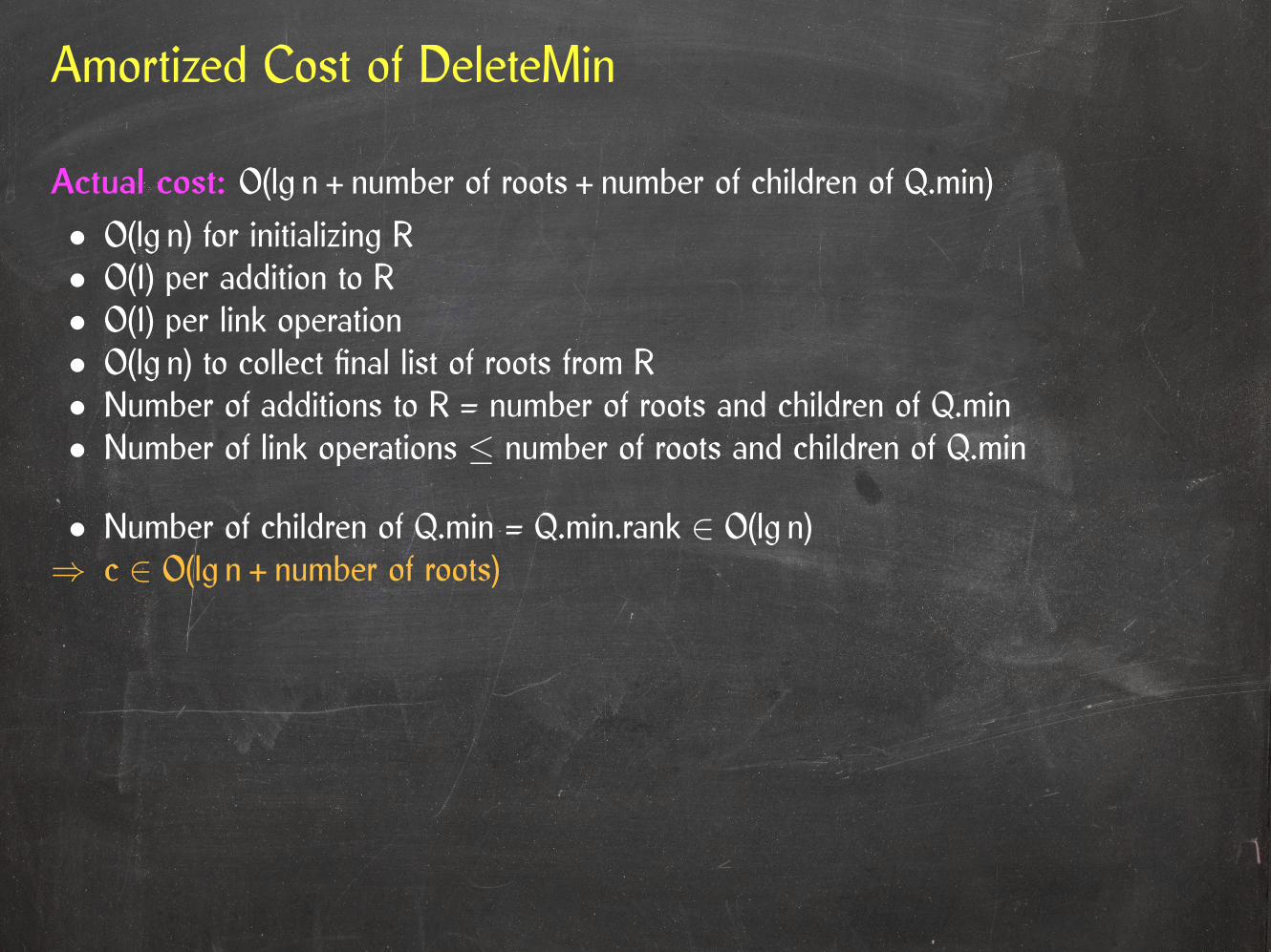
Actual cost: O(lg n + number of roots + number of children of Q.min)
• O(lg n) for initializing R• O(1) per addition to R• O(1) per link operation• O(lg n) to collect final list of roots from R• Number of additions to R = number of roots and children of Q.min• Number of link operations ≤ number of roots and children of Q.min
• Number of children of Q.min = Q.min.rank ∈ O(lg n)⇒ c ∈ O(lg n + number of roots)
Amortized Cost of DeleteMin
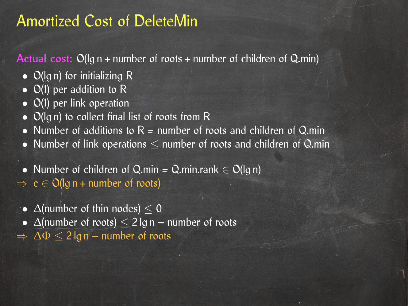
Actual cost: O(lg n + number of roots + number of children of Q.min)
• O(lg n) for initializing R• O(1) per addition to R• O(1) per link operation• O(lg n) to collect final list of roots from R• Number of additions to R = number of roots and children of Q.min• Number of link operations ≤ number of roots and children of Q.min
• Number of children of Q.min = Q.min.rank ∈ O(lg n)⇒ c ∈ O(lg n + number of roots)
• ∆(number of thin nodes) ≤ 0• ∆(number of roots) ≤ 2 lg n – number of roots⇒ ∆Φ ≤ 2 lg n – number of roots
Amortized Cost of DeleteMin
Actual cost: O(lg n + number of roots + number of children of Q.min)
• O(lg n) for initializing R• O(1) per addition to R• O(1) per link operation• O(lg n) to collect final list of roots from R• Number of additions to R = number of roots and children of Q.min• Number of link operations ≤ number of roots and children of Q.min
• Number of children of Q.min = Q.min.rank ∈ O(lg n)⇒ c ∈ O(lg n + number of roots)
• ∆(number of thin nodes) ≤ 0• ∆(number of roots) ≤ 2 lg n – number of roots⇒ ∆Φ ≤ 2 lg n – number of roots
Amortized cost:c = c + ∆Φ = O(lg n + number of roots) + 2 lg n – number of roots ∈ O(lg n).
Amortized Cost of DecreaseKey
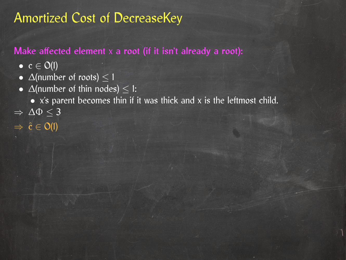
Make a�ected element x a root (if it isn’t already a root):
• c ∈ O(1)• ∆(number of roots) ≤ 1• ∆(number of thin nodes) ≤ 1:• x’s parent becomes thin if it was thick and x is the leftmost child.
⇒ ∆Φ ≤ 3
⇒ c ∈ O(1)
Amortized Cost of DecreaseKey
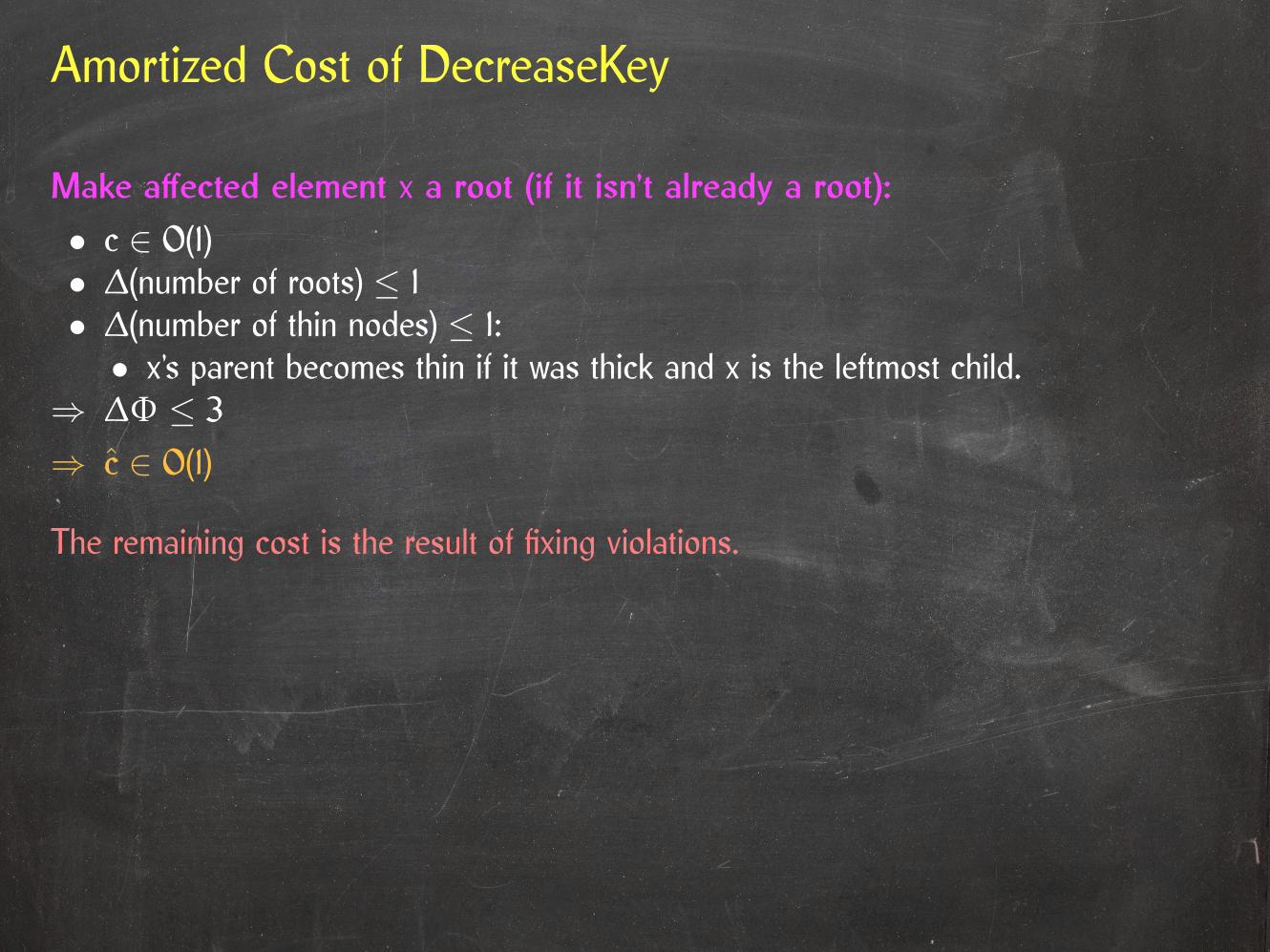
Make a�ected element x a root (if it isn’t already a root):
• c ∈ O(1)• ∆(number of roots) ≤ 1• ∆(number of thin nodes) ≤ 1:• x’s parent becomes thin if it was thick and x is the leftmost child.
⇒ ∆Φ ≤ 3
⇒ c ∈ O(1)
The remaining cost is the result of fixing violations.

Amortized Cost of DecreaseKey
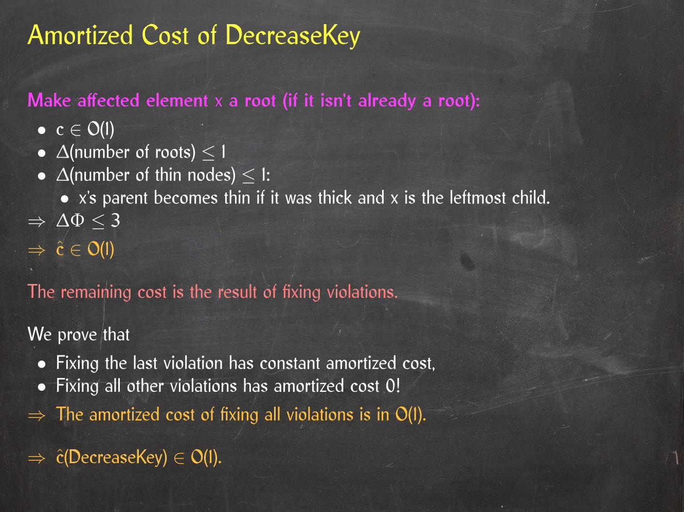
Make a�ected element x a root (if it isn’t already a root):
• c ∈ O(1)• ∆(number of roots) ≤ 1• ∆(number of thin nodes) ≤ 1:• x’s parent becomes thin if it was thick and x is the leftmost child.
⇒ ∆Φ ≤ 3
⇒ c ∈ O(1)
The remaining cost is the result of fixing violations.
We prove that
• Fixing the last violation has constant amortized cost,• Fixing all other violations has amortized cost 0!
⇒ The amortized cost of fixing all violations is in O(1).
Amortized Cost of DecreaseKey
Make a�ected element x a root (if it isn’t already a root):
• c ∈ O(1)• ∆(number of roots) ≤ 1• ∆(number of thin nodes) ≤ 1:• x’s parent becomes thin if it was thick and x is the leftmost child.
⇒ ∆Φ ≤ 3
⇒ c ∈ O(1)
The remaining cost is the result of fixing violations.
We prove that
• Fixing the last violation has constant amortized cost,• Fixing all other violations has amortized cost 0!
⇒ The amortized cost of fixing all violations is in O(1).
⇒ c(DecreaseKey) ∈ O(1).
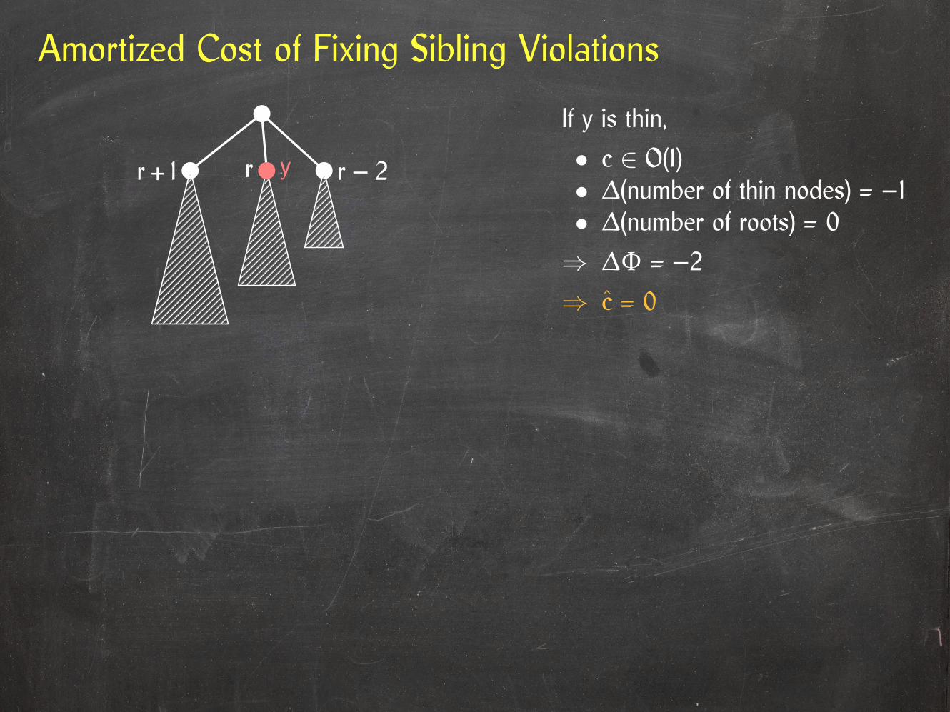
Amortized Cost of Fixing Sibling Violations
r + 1 r – 2yr
If y is thin,
• c ∈ O(1)• ∆(number of thin nodes) = –1• ∆(number of roots) = 0
⇒ ∆Φ = –2
⇒ c = 0

Amortized Cost of Fixing Sibling Violations
r – 1 r – 2
r r – 1 r – 2y
r + 1 r – 2yr
If y is thin,
• c ∈ O(1)• ∆(number of thin nodes) = –1• ∆(number of roots) = 0
⇒ ∆Φ = –2
⇒ c = 0
If y is thick,
• c ∈ O(1)• ∆(number of thin nodes) = +1• ∆(number of roots) = 0
⇒ ∆Φ = +2
⇒ c ∈ O(1)
After this, we’re done!

Amortized Cost of Fixing Parent Violations
y
< r – 2
r
If y is a root, then
• c ∈ O(1)• ∆(number of roots) = 0• ∆(number of thin nodes) = –1
⇒ ∆Φ = –2
⇒ c = 0

Amortized Cost of Fixing Parent Violations
y
< r – 2
r
If y is a root, then
• c ∈ O(1)• ∆(number of roots) = 0• ∆(number of thin nodes) = –1
⇒ ∆Φ = –2
⇒ c = 0
If y is not a root and is not the leftmost child of itsparent, then
• c ∈ O(1)• ∆(number of roots) = +1• ∆(number of thin nodes) = –1
⇒ ∆Φ = –1
⇒ c = 0

Amortized Cost of Fixing Parent Violations
y
< r – 2
r
If y is not a root and is the leftmost child of itsparent, and its parent is thin, then
• c ∈ O(1)• ∆(number of roots) = +1• ∆(number of thin nodes) = –1
⇒ ∆Φ = –1
⇒ c = 0

Amortized Cost of Fixing Parent Violations
y
< r – 2
r
If y is not a root and is the leftmost child of itsparent, and its parent is thin, then
• c ∈ O(1)• ∆(number of roots) = +1• ∆(number of thin nodes) = –1
⇒ ∆Φ = –1
⇒ c = 0
If y is not a root and is the leftmost child of itsparent, and its parent is thick, then
• c ∈ O(1)• ∆(number of roots) = +1• ∆(number of thin nodes) = 0
⇒ ∆Φ = +1
⇒ c ∈ O(1)
After this, we’re done!

Shortest Path
Given a graph G = (V, E) and an assignment of weights (costs) to the edges of G, ashortest path from u to v is a path from u to v with minimum total edge weight amongall paths from u to v.
6
1
3
5
4
7
8
3
1
2
97
6
3

Shortest Path
Given a graph G = (V, E) and an assignment of weights (costs) to the edges of G, ashortest path from u to v is a path from u to v with minimum total edge weight amongall paths from u to v.
6
1
3
5
4
7
8
3
1
2
97
6
3
Let the distance dist(s, w) from s to v be the length of a shortest path from s to v.

Shortest Path
Given a graph G = (V, E) and an assignment of weights (costs) to the edges of G, ashortest path from u to v is a path from u to v with minimum total edge weight amongall paths from u to v.
This is well-defined only if there is no negative cycle (cycle with negative total edgeweight) that has a vertex on a path from u to v.
6
1
3
5
4
7
8
3
1
2
97
6
3
Let the distance dist(s, w) from s to v be the length of a shortest path from s to v.

Optimal Substructure of Shortest Paths
For a path P and two vertices u and w in P, let P[u, w] be the subpath of P from u to w.
P
P[u, w]

Optimal Substructure of Shortest Paths
For a path P and two vertices u and w in P, let P[u, w] be the subpath of P from u to w.
Lemma: If Pv is a shortest path from s to v and w is a vertex in Pv, then Pv[s, w] is ashortest path from s to w.
P
P[u, w]
s
w
v
Pv[s, w]P[w, v]

Optimal Substructure of Shortest Paths
For a path P and two vertices u and w in P, let P[u, w] be the subpath of P from u to w.
Lemma: If Pv is a shortest path from s to v and w is a vertex in Pv, then Pv[s, w] is ashortest path from s to w.
Assume there exists a path Pw from s to w with w(Pw) < w(Pv[s, w]).
P
P[u, w]
s
w
vPw
Pv[s, w]P[w, v]

Optimal Substructure of Shortest Paths
For a path P and two vertices u and w in P, let P[u, w] be the subpath of P from u to w.
Lemma: If Pv is a shortest path from s to v and w is a vertex in Pv, then Pv[s, w] is ashortest path from s to w.
Assume there exists a path Pw from s to w with w(Pw) < w(Pv[s, w]).
Then w(Pw ◦ Pv[w, v]) < w(Pv[s, w] ◦ Pv[w, v]) = w(Pv), a contradiction because Pv is ashortest path from s to v.
P
P[u, w]
s
w
vPw
Pv[s, w]P[w, v]

Shortest Path Tree
Lemma: For every node s ∈ G, there exists a collection of paths S = {Pv | v ∈ R(s)}such that Pv is a shortest path from s to v and
⋃v∈R(s) Pv is a tree.
For a vertex s ∈ G, let R(s) be the set of vertices reachable from s: for every vertexv ∈ R(s), there exists a path from s to v.
6
1
3
5
4
7
8
3
1
2
97
6
3
s

Shortest Path Tree
Lemma: For every node s ∈ G, there exists a collection of paths S = {Pv | v ∈ R(s)}such that Pv is a shortest path from s to v and
⋃v∈R(s) Pv is a tree.
For a vertex s ∈ G, let R(s) be the set of vertices reachable from s: for every vertexv ∈ R(s), there exists a path from s to v.
Let R(s) = {v1, v2, . . . , vt} and let {P′v1 , P′v2 , . . . , P
′vt } be a
collection of shortest paths from s to these vertices.
We define a sequence of trees 〈T1, T2, . . . , Tt〉and shortest paths 〈Pv1 , Pv2 , . . . , Pvt〉 as follows:
v2
v4
s
v1
v3

Shortest Path Tree
Lemma: For every node s ∈ G, there exists a collection of paths S = {Pv | v ∈ R(s)}such that Pv is a shortest path from s to v and
⋃v∈R(s) Pv is a tree.
For a vertex s ∈ G, let R(s) be the set of vertices reachable from s: for every vertexv ∈ R(s), there exists a path from s to v.
Let R(s) = {v1, v2, . . . , vt} and let {P′v1 , P′v2 , . . . , P
′vt } be a
collection of shortest paths from s to these vertices.
We define a sequence of trees 〈T1, T2, . . . , Tt〉and shortest paths 〈Pv1 , Pv2 , . . . , Pvt〉 as follows:
• T1 = Pv1 = P′v1 .
• For i > 0, let w be the last vertex in P′vi thatbelongs to Ti–1 and let Ti–1[s, w] be the pathfrom s to w in T. Then
• Pvi = T[s, w] ◦ P′vi [w, vi]• Ti = Ti–1
⋃P′vi [w, vi]
v2
v4
s
v1
v3

Shortest Path Tree
Lemma: For every node s ∈ G, there exists a collection of paths S = {Pv | v ∈ R(s)}such that Pv is a shortest path from s to v and
⋃v∈R(s) Pv is a tree.
For a vertex s ∈ G, let R(s) be the set of vertices reachable from s: for every vertexv ∈ R(s), there exists a path from s to v.
v2
v4
s
v1
v3
Tt =⋃
v∈R(s) Pv
Tt is a tree:
• T1 is a tree.
• Ti is obtained by adding a path to Ti–1 thatshares only one vertex with Ti–1.
• To create a cycle, the added path would haveto share two vertices with Ti–1.

Shortest Path Tree
Lemma: For every node s ∈ G, there exists a collection of paths S = {Pv | v ∈ R(s)}such that Pv is a shortest path from s to v and
⋃v∈R(s) Pv is a tree.
For a vertex s ∈ G, let R(s) be the set of vertices reachable from s: for every vertexv ∈ R(s), there exists a path from s to v.
v2
v4
s
v1
v3
Pv is a shortest path from s to v, for all v ∈ R(s).
Prove by induction on i that Ti[s, v] is a shortestpath from s to v, for all v ∈ Ti.

Shortest Path Tree
Lemma: For every node s ∈ G, there exists a collection of paths S = {Pv | v ∈ R(s)}such that Pv is a shortest path from s to v and
⋃v∈R(s) Pv is a tree.
For a vertex s ∈ G, let R(s) be the set of vertices reachable from s: for every vertexv ∈ R(s), there exists a path from s to v.
v2
v4
s
v1
v3
Pv is a shortest path from s to v, for all v ∈ R(s).
For i = 1, T1 = Pv1 = P′v1 is a shortest path from sto v1. By optimal substructure, T1[s, v] = P′v1 [s, v]is a shortest path from s to v for all v ∈ T1.
For i > 1, Ti–1[s, v] is a shortest path from s to vfor all v ∈ Ti–1, by the inductive hypothesis.
Thus, w(Ti–1[s, w]) ≤ w(P′vi [s, w]) and thereforew(Pvi ) = w(Ti–1[s, w]) + w(P
′vi [w, vi]) ≤ w(P′vi ).
Since P′vi is a shortest path from s to vi, so is Pvi .
By optimal substructure Pvi [s, v] is a shortestpath from s to v, for all v ∈ Pvi .

A Characterization of Shortest Path TreesAn out-tree of s is a spanning tree T of G[R(s)] = (R(s), E[R(s)]), whereE[R(s)] = {(v, w) ∈ E | v, w ∈ R(s)}, such that there exists a path from s to v in T, for allv ∈ R(s).
s

A Characterization of Shortest Path TreesAn out-tree of s is a spanning tree T of G[R(s)] = (R(s), E[R(s)]), whereE[R(s)] = {(v, w) ∈ E | v, w ∈ R(s)}, such that there exists a path from s to v in T, for allv ∈ R(s).
For an out-tree T of s and every v ∈ T, let dT(v) = w(T[s, v]).
s

A Characterization of Shortest Path TreesAn out-tree of s is a spanning tree T of G[R(s)] = (R(s), E[R(s)]), whereE[R(s)] = {(v, w) ∈ E | v, w ∈ R(s)}, such that there exists a path from s to v in T, for allv ∈ R(s).
For an out-tree T of s and every v ∈ T, let dT(v) = w(T[s, v]).
Let D(T) =∑v∈R(s)
dT(v).
s

A Characterization of Shortest Path TreesAn out-tree of s is a spanning tree T of G[R(s)] = (R(s), E[R(s)]), whereE[R(s)] = {(v, w) ∈ E | v, w ∈ R(s)}, such that there exists a path from s to v in T, for allv ∈ R(s).
Lemma: An out-tree T of s is a shortest path tree if and only if D(T) is minimalamong all out-trees of s.
For an out-tree T of s and every v ∈ T, let dT(v) = w(T[s, v]).
Let D(T) =∑v∈R(s)
dT(v).
Let T and T′ be two out-trees of s such that• T is a shortest path tree and• D(T′) is minimal among all out-trees of s. In particular, D(T′) ≤ D(T).
If D(T′) < D(T), there exists some vertex v ∈ R(s) such that dT′ (v) < dT(v).
⇒ T is not a shortest path tree, a contradiction.
⇒ D(T) = D(T′).

A Characterization of Shortest Path TreesAn out-tree of s is a spanning tree T of G[R(s)] = (R(s), E[R(s)]), whereE[R(s)] = {(v, w) ∈ E | v, w ∈ R(s)}, such that there exists a path from s to v in T, for allv ∈ R(s).
Lemma: An out-tree T of s is a shortest path tree if and only if D(T) is minimalamong all out-trees of s.
For an out-tree T of s and every v ∈ T, let dT(v) = w(T[s, v]).
Let D(T) =∑v∈R(s)
dT(v).
Let T and T′ be two out-trees of s such that D(T) = D(T′) is minimal among allout-trees of s and• T is a shortest path tree,• T′ is not.
⇒ There exists a vertex v ∈ R(s) such that dT(v) < dT′ (v).
⇒ There exists a vertex v′ ∈ R(s) such that dT′ (v′) < dT(v′), a contradiction.
⇒ T′ is a shortest path tree.

Dijkstra’s Algorithm
Build a shortest-path tree by starting with s and adding vertices in R(s) one by one.

Dijkstra’s Algorithm
Build a shortest-path tree by starting with s and adding vertices in R(s) one by one.
In each step, we can only add out-neighbours of vertices already in T.

Dijkstra’s Algorithm
Build a shortest-path tree by starting with s and adding vertices in R(s) one by one.
In each step, we can only add out-neighbours of vertices already in T.
A greedy choice:
Add the vertex v 6∈ T that minimizes dT(v).

Dijkstra’s Algorithm
Build a shortest-path tree by starting with s and adding vertices in R(s) one by one.
In each step, we can only add out-neighbours of vertices already in T.
A greedy choice:
Add the vertex v 6∈ T that minimizes dT(v).
Dijkstra(G, s)
1 T = ({s}, ∅)2 while some vertex in T has an out-neighbour not in T3 do choose an edge (u, v) such that
• u ∈ T,• v 6∈ T, and• dT(u) + w(u, v) is minimized.
4 add v and (u, v) to T5 return T

Dijkstra’s AlgorithmDijkstra(G, s)
1 T = (V, ∅)2 mark every vertex of G as unexplored3 set d(v) = +∞ and e(v) = nil for every vertex v ∈ G4 mark s as explored and set d(v) = 05 Q = an empty priority queue6 for every edge (s, v) incident to s7 do Q.insert(v, w(s, v))8 d(v) = w(s, v)9 e(v) = (s, v)10 while not Q.isEmpty()11 do u = Q.deleteMin()12 mark u as explored13 add e(u) to T14 for every edge (u, v) incident to u15 do if v is unexplored and (v 6∈ Q or d(u) + w(u, v) < d(v))16 then d(v) = d(u) + w(u, v)17 e(v) = (u, v)18 if v 6∈ Q19 then Q.insert(v, d(v))20 else Q.decreaseKey(v, d(v))21 return T
This is the same as Prim’salgorithm, except that vertexpriorities are calculateddi�erently.
⇒ Dijkstra’s algorithm takesO(n lg n + m) time.

Correctness of Dijkstra’s Algorithm
Dijkstra’s algorithm does not necessarily produce a shortest path tree if there areedges with negative weights!

Correctness of Dijkstra’s Algorithm
Dijkstra’s algorithm does not necessarily produce a shortest path tree if there areedges with negative weights!
Lemma: If all edges in G have non-negative weights, then Dijkstra’s algorithmcomputes a shortest path tree of G.

Correctness of Dijkstra’s Algorithm
Dijkstra’s algorithm does not necessarily produce a shortest path tree if there areedges with negative weights!
Lemma: If all edges in G have non-negative weights, then Dijkstra’s algorithmcomputes a shortest path tree of G.
Assume the contrary and let v be the first vertex added to T such that dT(v) > dist(s, v).
For every vertex x 6∈ T, we have
d(x) = min(u,x)∈Eu∈T
d(u) + w(u, x) = min(u,x)∈Eu∈T
dist(s, u) + w(u, x).
sx

Correctness of Dijkstra’s Algorithm
Dijkstra’s algorithm does not necessarily produce a shortest path tree if there areedges with negative weights!
Lemma: If all edges in G have non-negative weights, then Dijkstra’s algorithmcomputes a shortest path tree of G.
Assume the contrary and let v be the first vertex added to T such that dT(v) > dist(s, v).
The shortest path π(s, v) from s to v must include a vertex w 6∈ T whose predecessoru in π(s, v) belongs to T.
wu
sv
T
π(s, v)
d(v)

Correctness of Dijkstra’s Algorithm
Dijkstra’s algorithm does not necessarily produce a shortest path tree if there areedges with negative weights!
Lemma: If all edges in G have non-negative weights, then Dijkstra’s algorithmcomputes a shortest path tree of G.
Assume the contrary and let v be the first vertex added to T such that dT(v) > dist(s, v).
The shortest path π(s, v) from s to v must include a vertex w 6∈ T whose predecessoru in π(s, v) belongs to T.
⇒ d(w) ≤ dist(s, u) + w(u, w) = dist(s, w) ≤ dist(s, v) < d(v).
⇒ v is not the next vertex we add to T, a contradiction.
wu
sv
T
π(s, v)
d(v)

Minimum Length Codes
This is atext to beencoded.
010101011100011100101010000110111001101This is atext to beencoded.
01010101110
0011100
10101000
Goal:
• Encode a given text using as few bits as possible:• Limit amount of disk space required to store
the text.• Send the text over a potentially slow network.• . . .

Codes That Can Be Decoded
A code is a mapping C(·) that maps every character x to a bit string C(x), called theencoding of x.

Codes That Can Be Decoded
A code is a mapping C(·) that maps every character x to a bit string C(x), called theencoding of x.
e f i p r x -C1 000 001 010 011 100 101 110

Codes That Can Be Decoded
A code is a mapping C(·) that maps every character x to a bit string C(x), called theencoding of x.
For a text T = 〈x1, x2, . . . , xn〉, let C(T) = C(x1) ◦ C(x2) ◦ · · · ◦ C(xn) be the bit stringobtained by concatenating the encodings of its characters. We call C(T) the encodingof T.
“prefix-free”
e f i p r x -C1 000 001 010 011 100 101 110
C1(prefix-free) = 011 100 000 001 010 101 110 001 100 000 000 (33 bits)

Codes That Can Be Decoded
A code is a mapping C(·) that maps every character x to a bit string C(x), called theencoding of x.
For a text T = 〈x1, x2, . . . , xn〉, let C(T) = C(x1) ◦ C(x2) ◦ · · · ◦ C(xn) be the bit stringobtained by concatenating the encodings of its characters. We call C(T) the encodingof T.
“prefix-free”
e f i p r x -C1 000 001 010 011 100 101 110C2 00 010 0110 0111 10 110 111
C1(prefix-free) = 011 100 000 001 010 101 110 001 100 000 000 (33 bits)
C2(prefix-free) = 0111 10 00 010 0110 110 111 010 10 00 00 (30 bits)

Codes That Can Be Decoded
A code is a mapping C(·) that maps every character x to a bit string C(x), called theencoding of x.
For a text T = 〈x1, x2, . . . , xn〉, let C(T) = C(x1) ◦ C(x2) ◦ · · · ◦ C(xn) be the bit stringobtained by concatenating the encodings of its characters. We call C(T) the encodingof T.
“prefix-free”
C1(prefix-free) = 011 100 000 001 010 101 110 001 100 000 000 (33 bits)
C2(prefix-free) = 0111 10 00 010 0110 110 111 010 10 00 00 (30 bits)
C3(prefix-free) = 01 10 0 1 00 11 000 1 10 0 0 (18 bits)
e f i p r x -C1 000 001 010 011 100 101 110C2 00 010 0110 0111 10 110 111C3 0 1 00 01 10 11 000

Codes That Can Be Decoded
A code is a mapping C(·) that maps every character x to a bit string C(x), called theencoding of x.
A code C(·) is prefix-free if there are no two characters x and y such that C(x) is aprefix of C(y).
Non-prefix-free codes cannot always be decoded uniquely!
For a text T = 〈x1, x2, . . . , xn〉, let C(T) = C(x1) ◦ C(x2) ◦ · · · ◦ C(xn) be the bit stringobtained by concatenating the encodings of its characters. We call C(T) the encodingof T.
“prefix-free”
C1(prefix-free) = 011 100 000 001 010 101 110 001 100 000 000 (33 bits)
C2(prefix-free) = 0111 10 00 010 0110 110 111 010 10 00 00 (30 bits)
C3(prefix-free) = 01 10 0 1 00 11 000 1 10 0 0 (18 bits)
e f i p r x -C1 000 001 010 011 100 101 110C2 00 010 0110 0111 10 110 111C3 0 1 00 01 10 11 000

Codes That Can Be Decoded
Lemma: If C(·) is a prefix-free code and T 6= T′, then C(T) 6= C(T′).

Codes That Can Be Decoded
Lemma: If C(·) is a prefix-free code and T 6= T′, then C(T) 6= C(T′).
Let T = 〈x1, x2, . . . , xm〉 and T′ = 〈y1, y2, . . . , yn〉 and assume C(T) = C(T′).
C(T)
C(T′)

Codes That Can Be Decoded
Lemma: If C(·) is a prefix-free code and T 6= T′, then C(T) 6= C(T′).
Let T = 〈x1, x2, . . . , xm〉 and T′ = 〈y1, y2, . . . , yn〉 and assume C(T) = C(T′).
Let i be the minimum index such that xi 6= yi.
C(T)
C(T′)

Codes That Can Be Decoded
Lemma: If C(·) is a prefix-free code and T 6= T′, then C(T) 6= C(T′).
Let T = 〈x1, x2, . . . , xm〉 and T′ = 〈y1, y2, . . . , yn〉 and assume C(T) = C(T′).
Let i be the minimum index such that xi 6= yi.
⇒ C(〈x1, x2, . . . , xi–1〉) = C(〈y1, y2, . . . , yi–1〉) andC(〈xi, xi+1, . . . , xm〉) = C(〈yi, yi+1, . . . , yn〉).
C(T)
C(T′) C(〈y1, y2, . . . , yi–1〉) C(〈yi+1, yi+2, . . . , yn〉)C(yi)
C(〈x1, x2, . . . , xi–1〉) C(〈xi+1, xi+2, . . . , xm〉)C(xi)

Codes That Can Be Decoded
Lemma: If C(·) is a prefix-free code and T 6= T′, then C(T) 6= C(T′).
Let T = 〈x1, x2, . . . , xm〉 and T′ = 〈y1, y2, . . . , yn〉 and assume C(T) = C(T′).
Let i be the minimum index such that xi 6= yi.
⇒ C(〈x1, x2, . . . , xi–1〉) = C(〈y1, y2, . . . , yi–1〉) andC(〈xi, xi+1, . . . , xm〉) = C(〈yi, yi+1, . . . , yn〉).
Assume w.l.o.g. that |C(xi)| ≤ |C(yi)|.
Since both C(xi) and C(yi) are prefixes of C(〈xi, xi+1, . . . , xm〉), C(xi) must be a prefix ofC(yi), a contradiction.
C(T)
C(T′) C(〈y1, y2, . . . , yi–1〉) C(〈yi+1, yi+2, . . . , yn〉)C(yi)
C(〈x1, x2, . . . , xi–1〉) C(〈xi+1, xi+2, . . . , xm〉)C(xi)

Prefix Codes and Binary Trees
Observation: Every prefix-free code C(·) can be represented as a binary tree TCwhose leaves correspond to the le�ers in the alphabet.
e f i p r x -C 00 010 0110 0111 10 110 111
0
1
1
1
1
1
10
0
0
0
0e
f
i
x
p
r
-

Prefix Codes and Binary Trees
The depth of character x in TC is the number of bits |C(x)| used to encode x using C(·).
Observation: Every prefix-free code C(·) can be represented as a binary tree TCwhose leaves correspond to the le�ers in the alphabet.
e f i p r x -C 00 010 0110 0111 10 110 111
0
1
1
1
1
1
10
0
0
0
0e
f
i
x
p
r
-

Optimal Prefix Codes and Binary Trees
An optimal prefix-free code for a text T is a prefix-free code C that minimizes |C(T)|.

Optimal Prefix Codes and Binary Trees
An optimal prefix-free code for a text T is a prefix-free code C that minimizes |C(T)|.
Lemma: For every text T, there exists an optimal prefix-free code C(·) such that everyinternal node in TC has two children.
TC x1
x2
x3 x6x4
x5
x7
v

Optimal Prefix Codes and Binary Trees
An optimal prefix-free code for a text T is a prefix-free code C that minimizes |C(T)|.
Lemma: For every text T, there exists an optimal prefix-free code C(·) such that everyinternal node in TC has two children.
Choose C(·) so that TC has as few internalnodes with only one child as possible amongall optimal prefix-free codes for T.
If TC has no internal node with only one child,the lemma holds.
Otherwise, choose an internal node v withonly one child w and contract the edge (v, w).
TC x1
x2
x3 x6x4
x5
x7
TC′ x1
x2
x3
x6
x4
x5
x7
v

Optimal Prefix Codes and Binary Trees
An optimal prefix-free code for a text T is a prefix-free code C that minimizes |C(T)|.
Lemma: For every text T, there exists an optimal prefix-free code C(·) such that everyinternal node in TC has two children.
Choose C(·) so that TC has as few internalnodes with only one child as possible amongall optimal prefix-free codes for T.
If TC has no internal node with only one child,the lemma holds.
Otherwise, choose an internal node v withonly one child w and contract the edge (v, w).
The resulting tree TC′ has one less internalnode with only one child and represents aprefix-free code C′(·) with the property that|C′(x)| ≤ |C(x)| for every character x.
⇒ |C′(T)| ≤ |C(T)|, contradicting the choice of C.
TC x1
x2
x3 x6x4
x5
x7
TC′ x1
x2
x3
x6
x4
x5
x7
v

A Greedy Choice for Optimal Prefix CodesWe can build binary trees by starting with each leaf in its own tree, joining two treesunder a common parent, and repeating this until only one tree is left.

A Greedy Choice for Optimal Prefix CodesWe can build binary trees by starting with each leaf in its own tree, joining two treesunder a common parent, and repeating this until only one tree is left.
e f i xp r -

A Greedy Choice for Optimal Prefix CodesWe can build binary trees by starting with each leaf in its own tree, joining two treesunder a common parent, and repeating this until only one tree is left.
e f i xp r -

A Greedy Choice for Optimal Prefix CodesWe can build binary trees by starting with each leaf in its own tree, joining two treesunder a common parent, and repeating this until only one tree is left.
e f i xp r -

A Greedy Choice for Optimal Prefix CodesWe can build binary trees by starting with each leaf in its own tree, joining two treesunder a common parent, and repeating this until only one tree is left.
e i xp r -
f

A Greedy Choice for Optimal Prefix CodesWe can build binary trees by starting with each leaf in its own tree, joining two treesunder a common parent, and repeating this until only one tree is left.
e i xp
r
-
f

A Greedy Choice for Optimal Prefix CodesWe can build binary trees by starting with each leaf in its own tree, joining two treesunder a common parent, and repeating this until only one tree is left.
i xp
r
-
f
e

A Greedy Choice for Optimal Prefix CodesWe can build binary trees by starting with each leaf in its own tree, joining two treesunder a common parent, and repeating this until only one tree is left.
e
f
i
x
p
r
-

A Greedy Choice for Optimal Prefix CodesWe can build binary trees by starting with each leaf in its own tree, joining two treesunder a common parent, and repeating this until only one tree is left.
The length of the encoding of T is |C(T)| =∑
x fT(x)|C(x)|, where fT(x) is the frequencyof x in T.
e
f
i
x
p
r
-

A Greedy Choice for Optimal Prefix CodesWe can build binary trees by starting with each leaf in its own tree, joining two treesunder a common parent, and repeating this until only one tree is left.
The length of the encoding of T is |C(T)| =∑
x fT(x)|C(x)|, where fT(x) is the frequencyof x in T.When making a node r a child of a new parent, we add 1 bit to the encoding C(x) ofevery descendant leaf x of r.
⇒ By choosing the two roots with minimum total frequency of their descendentleaves, we minimize the increase in |C(T)|.
“prefix-free”
x e f i p r x -fT(x) 3 2 1 1 2 1 1
e (3) f (2) i (1) x (1)p (1) r (2) - (1)
(2)

A Greedy Choice for Optimal Prefix CodesWe can build binary trees by starting with each leaf in its own tree, joining two treesunder a common parent, and repeating this until only one tree is left.
The length of the encoding of T is |C(T)| =∑
x fT(x)|C(x)|, where fT(x) is the frequencyof x in T.When making a node r a child of a new parent, we add 1 bit to the encoding C(x) ofevery descendant leaf x of r.
⇒ By choosing the two roots with minimum total frequency of their descendentleaves, we minimize the increase in |C(T)|.
“prefix-free”
x e f i p r x -fT(x) 3 2 1 1 2 1 1
e (3) f (2) i (1) x (1)p (1) r (2) - (1)
(2) (2)

A Greedy Choice for Optimal Prefix CodesWe can build binary trees by starting with each leaf in its own tree, joining two treesunder a common parent, and repeating this until only one tree is left.
The length of the encoding of T is |C(T)| =∑
x fT(x)|C(x)|, where fT(x) is the frequencyof x in T.When making a node r a child of a new parent, we add 1 bit to the encoding C(x) ofevery descendant leaf x of r.
⇒ By choosing the two roots with minimum total frequency of their descendentleaves, we minimize the increase in |C(T)|.
“prefix-free”
x e f i p r x -fT(x) 3 2 1 1 2 1 1
e (3)
f (2)
i (1) x (1)p (1) r (2) - (1)
(2) (2)
(4)

A Greedy Choice for Optimal Prefix CodesWe can build binary trees by starting with each leaf in its own tree, joining two treesunder a common parent, and repeating this until only one tree is left.
The length of the encoding of T is |C(T)| =∑
x fT(x)|C(x)|, where fT(x) is the frequencyof x in T.When making a node r a child of a new parent, we add 1 bit to the encoding C(x) ofevery descendant leaf x of r.
⇒ By choosing the two roots with minimum total frequency of their descendentleaves, we minimize the increase in |C(T)|.
“prefix-free”
x e f i p r x -fT(x) 3 2 1 1 2 1 1
e (3)
f (2)
i (1) x (1)p (1)
r (2)
- (1)
(2) (2)
(4) (4)
(7)

A Greedy Choice for Optimal Prefix CodesWe can build binary trees by starting with each leaf in its own tree, joining two treesunder a common parent, and repeating this until only one tree is left.
The length of the encoding of T is |C(T)| =∑
x fT(x)|C(x)|, where fT(x) is the frequencyof x in T.When making a node r a child of a new parent, we add 1 bit to the encoding C(x) ofevery descendant leaf x of r.
⇒ By choosing the two roots with minimum total frequency of their descendentleaves, we minimize the increase in |C(T)|.
“prefix-free”
x e f i p r x -fT(x) 3 2 1 1 2 1 1
e (3)
f (2)
i (1)
x (1)
p (1)
r (2)
- (1)(2)
(2)(4)
(4)(7)
(11)

Hu�man’s Algorithm
Hu�man(T)
1 determine the set A of characters that occur in T and their frequencies2 Q = an empty priority queue3 for every character x ∈ A4 do create a node v associated with x and define f(v) = f(x)5 Q.insert(v, f(v))6 while |Q| > 17 do v = Q.deleteMin()8 w = Q.deleteMin()9 u = a new node with frequency f(u) = f(v) + f(w)10 make v and w children of u11 Q.insert(u, f(u))12 return Q.deleteMin()
Lemma: Hu�man’s algorithm runs in O(m lg n) time, where m = |T| and n is the size ofthe alphabet.

Correctness of Hu�man’s AlgorithmLemma: Hu�man’s algorithm computes an optimal prefix-free code for its input text T.

Correctness of Hu�man’s AlgorithmLemma: Hu�man’s algorithm computes an optimal prefix-free code for its input text T.
Proof by induction on n.

Correctness of Hu�man’s AlgorithmLemma: Hu�man’s algorithm computes an optimal prefix-free code for its input text T.
Proof by induction on n.
Base case: n = 2.

Correctness of Hu�man’s AlgorithmLemma: Hu�man’s algorithm computes an optimal prefix-free code for its input text T.
Proof by induction on n.
Base case: n = 2.
We cannot do be�er than using one bit percharacter.

Correctness of Hu�man’s AlgorithmLemma: Hu�man’s algorithm computes an optimal prefix-free code for its input text T.
Proof by induction on n.
Base case: n = 2.
We cannot do be�er than using one bit percharacter.
Inductive step: n > 2.

Correctness of Hu�man’s Algorithm
λ (2)
Lemma: Hu�man’s algorithm computes an optimal prefix-free code for its input text T.
Proof by induction on n.
Base case: n = 2.
We cannot do be�er than using one bit percharacter.
Inductive step: n > 2.
Consider the first two characters a and b that arejoined under a common parent z with frequencyf(z) = f(a) + f(b).
e (3) f (2) i (1) x (1)p (1) r (2) - (1)

Correctness of Hu�man’s Algorithm
i (1) p (1)
Lemma: Hu�man’s algorithm computes an optimal prefix-free code for its input text T.
Proof by induction on n.
Base case: n = 2.
We cannot do be�er than using one bit percharacter.
Inductive step: n > 2.
Consider the first two characters a and b that arejoined under a common parent z with frequencyf(z) = f(a) + f(b).
Replacing a and b with z in T produces a new textT′ over an alphabet of size n – 1 where z hasfrequency f(z).
“prefix-free”
“zrefzx-free”⇓
z (2)
e (3) f (2) x (1)r (2) - (1)

Correctness of Hu�man’s AlgorithmLemma: Hu�man’s algorithm computes an optimal prefix-free code for its input text T.
Proof by induction on n.
Base case: n = 2.
We cannot do be�er than using one bit percharacter.
Inductive step: n > 2.
Consider the first two characters a and b that arejoined under a common parent z with frequencyf(z) = f(a) + f(b).
Replacing a and b with z in T produces a new textT′ over an alphabet of size n – 1 where z hasfrequency f(z).
After joining a and b under z, Hu�man’s algorithmbehaves exactly as if it was run on T′.
“prefix-free”
“zrefzx-free”⇓
e (3)
f (2)
i (1)
x (1)
p (1)
r (2)
- (1)z (2)

Correctness of Hu�man’s AlgorithmLemma: Hu�man’s algorithm computes an optimal prefix-free code for its input text T.
Proof by induction on n.
Base case: n = 2.
We cannot do be�er than using one bit percharacter.
Inductive step: n > 2.
Consider the first two characters a and b that arejoined under a common parent z with frequencyf(z) = f(a) + f(b).
Replacing a and b with z in T produces a new textT′ over an alphabet of size n – 1 where z hasfrequency f(z).
After joining a and b under z, Hu�man’s algorithmbehaves exactly as if it was run on T′.
By induction, it produces an optimal code C′(·) for T′.
“prefix-free”
“zrefzx-free”⇓
e (3)
f (2)
i (1)
x (1)
p (1)
r (2)
- (1)z (2)

Correctness of Hu�man’s AlgorithmClaim: There exists an optimal prefix-free code C(·) for T such that the two leastfrequent characters a and b in T are siblings in TC.

Correctness of Hu�man’s AlgorithmClaim: There exists an optimal prefix-free code C(·) for T such that the two leastfrequent characters a and b in T are siblings in TC.
⇒ Hu�man’s algorithm produces an optimal prefix-free code for T.

Correctness of Hu�man’s AlgorithmClaim: There exists an optimal prefix-free code C(·) for T such that the two leastfrequent characters a and b in T are siblings in TC.
⇒ Hu�man’s algorithm produces an optimal prefix-free code for T.
Assume there exists a be�er code C∗(·) such that aand b are siblings in TC∗ , that is, |C∗(T)| < |C(T)|.
“prefix-free”
e (3)
f (2)
i (1)
x (1)
p (1)
r (2)
- (1)z (2)

Correctness of Hu�man’s AlgorithmClaim: There exists an optimal prefix-free code C(·) for T such that the two leastfrequent characters a and b in T are siblings in TC.
⇒ Hu�man’s algorithm produces an optimal prefix-free code for T.
Assume there exists a be�er code C∗(·) such that aand b are siblings in TC∗ , that is, |C∗(T)| < |C(T)|.
Let C′′(·) be the code for T′ defined as
C′′(x) =
{C∗(x) x 6= zσ x = z and C∗(a) = σ0
e (3)
f (2)
i (1)
x (1)
p (1)
r (2)
- (1)z (2)
“prefix-free”
“zrefzx-free”⇓

Correctness of Hu�man’s AlgorithmClaim: There exists an optimal prefix-free code C(·) for T such that the two leastfrequent characters a and b in T are siblings in TC.
⇒ Hu�man’s algorithm produces an optimal prefix-free code for T.
Assume there exists a be�er code C∗(·) such that aand b are siblings in TC∗ , that is, |C∗(T)| < |C(T)|.
Let C′′(·) be the code for T′ defined as
C′′(x) =
{C∗(x) x 6= zσ x = z and C∗(a) = σ0
We also have
C′(x) =
{C(x) x 6= zσ x = z and C(a) = σ0
|C(T)| = |C′(T′)| + f(z) and |C∗(T)| = |C′′(T′)| + f(z).
⇒ |C′′(T′)| < |C′(T′)|, a contradiction because C′(·) is optimal for T′.
e (3)
f (2)
i (1)
x (1)
p (1)
r (2)
- (1)z (2)
“prefix-free”
“zrefzx-free”⇓

Correctness of Hu�man’s AlgorithmClaim: There exists an optimal prefix-free code C(·) for T such that the two leastfrequent characters a and b in T are siblings in TC.

Correctness of Hu�man’s Algorithm
Let C∗(·) be an optimal code for T.
Claim: There exists an optimal prefix-free code C(·) for T such that the two leastfrequent characters a and b in T are siblings in TC.

Correctness of Hu�man’s Algorithm
Let C∗(·) be an optimal code for T.
The sibling b′ of the deepest leaf a′ inTC∗ is also a leaf.
Claim: There exists an optimal prefix-free code C(·) for T such that the two leastfrequent characters a and b in T are siblings in TC.
TC∗
a b
a′ b′

Correctness of Hu�man’s Algorithm
Let C∗(·) be an optimal code for T.
The sibling b′ of the deepest leaf a′ inTC∗ is also a leaf.
We have |C∗(a)| ≤ |C∗(a′)| and|C∗(b)| ≤ |C∗(b′)|.
Claim: There exists an optimal prefix-free code C(·) for T such that the two leastfrequent characters a and b in T are siblings in TC.
TC∗
a b
a′ b′

Correctness of Hu�man’s Algorithm
Let C∗(·) be an optimal code for T.
The sibling b′ of the deepest leaf a′ inTC∗ is also a leaf.
Now assume f(a) ≤ f(b) and f(a′) ≤ f(b′).
Let C(·) be the code such that TC isobtained from TC∗ by swapping a and a′,and b and b′.
We have |C∗(a)| ≤ |C∗(a′)| and|C∗(b)| ≤ |C∗(b′)|.
We prove that |C(T)| ≤ |C∗(T)|, that is, C(·)is an optimal prefix-free code for T.
Since a and b are siblings in TC, thisproves the claim.
Claim: There exists an optimal prefix-free code C(·) for T such that the two leastfrequent characters a and b in T are siblings in TC.
TC∗
a b
a′ b′

Correctness of Hu�man’s AlgorithmClaim: There exists an optimal prefix-free code C(·) for T such that the two leastfrequent characters a and b in T are siblings in TC.
Given: |C∗(a)| ≤ |C∗(a′)|, |C∗(b)| ≤ |C∗(b′)|, f(a) ≤ f(b), and f(a′) ≤ f(b′).

Correctness of Hu�man’s AlgorithmClaim: There exists an optimal prefix-free code C(·) for T such that the two leastfrequent characters a and b in T are siblings in TC.
Given: |C∗(a)| ≤ |C∗(a′)|, |C∗(b)| ≤ |C∗(b′)|, f(a) ≤ f(b), and f(a′) ≤ f(b′).
⇒ f(a) ≤ f(a′) and f(b) ≤ f(b′).

Correctness of Hu�man’s AlgorithmClaim: There exists an optimal prefix-free code C(·) for T such that the two leastfrequent characters a and b in T are siblings in TC.
Given: |C∗(a)| ≤ |C∗(a′)|, |C∗(b)| ≤ |C∗(b′)|, f(a) ≤ f(b), and f(a′) ≤ f(b′).
⇒ f(a) ≤ f(a′) and f(b) ≤ f(b′).
|C(T)| – |C∗(T)| = f(a)|C(a)| + f(b)|C(b)| + f(a′)|C(a′)| + f(b′)|C(b′)| –
f(a)|C∗(a)| – f(b)|C∗(b)| – f(a′)|C∗(a′)| – f(b′)|C∗(b′)|
= f(a)|C∗(a′)| + f(b)|C∗(b′)| + f(a′)|C∗(a)| + f(b′)|C∗(b)| –
f(a)|C∗(a)| – f(b)|C∗(b)| – f(a′)|C∗(a′)| – f(b′)|C∗(b′)|
= (f(a) – f(a′)) (|C∗(a′)| – |C∗(a)|) + (f(b) – f(b′)) (|C∗(b′)| – |C∗(b)|)

Correctness of Hu�man’s AlgorithmClaim: There exists an optimal prefix-free code C(·) for T such that the two leastfrequent characters a and b in T are siblings in TC.
Given: |C∗(a)| ≤ |C∗(a′)|, |C∗(b)| ≤ |C∗(b′)|, f(a) ≤ f(b), and f(a′) ≤ f(b′).
⇒ f(a) ≤ f(a′) and f(b) ≤ f(b′).
|C(T)| – |C∗(T)| = f(a)|C(a)| + f(b)|C(b)| + f(a′)|C(a′)| + f(b′)|C(b′)| –
f(a)|C∗(a)| – f(b)|C∗(b)| – f(a′)|C∗(a′)| – f(b′)|C∗(b′)|
= f(a)|C∗(a′)| + f(b)|C∗(b′)| + f(a′)|C∗(a)| + f(b′)|C∗(b)| –
f(a)|C∗(a)| – f(b)|C∗(b)| – f(a′)|C∗(a′)| – f(b′)|C∗(b′)|
= (f(a) – f(a′))︸ ︷︷ ︸≤0
(|C∗(a′)| – |C∗(a)|)︸ ︷︷ ︸≥0
+ (f(b) – f(b′))︸ ︷︷ ︸≤0
(|C∗(b′)| – |C∗(b)|)︸ ︷︷ ︸≥0
≤ 0

Summary
Greedy algorithms make natural local choices in their search for a globally optimalsolution.
Many good heuristics are greedy:
• Simple• Work well in practice
Proof that a greedy algorithm finds an optimal solution:
• Induction• Exchange argument
Useful data structures:
• Union-find data structure• Thin Heap
Analysis of a sequence of data structure operations:
• Amortized analysis• Potential functions