gravit,ational wam detectar - eindhoven university of technology
TRANSCRIPT
Vibration Isolation of the GRAIL
Gravit,ational Wam Detectar
Feasibility study of a spherical resonant mass antenna
Master’s thesis
Author : T.G.H. Basten
Professor :
Mentors :
Date : Institution :
Report Number
Prof. Dr. Ir. D.H. van Campen
Prof. Dr. A.T.A.M de Waele Dr. Ir. A. de Kraker
September 1996 Eindhoven University of Technology Department of Mechanical Engineering Fundamentals of Mechanical Engineering (WFW)
W F W 96.135

Vibration Isolation of the GRAIL Gravitational Wave Detector
T.G.H. Basten

.. 11
.. 11

urnrnary
The detection of gravitational waves is a big challenge in experimental physics. In the Nether- lands a gravitational wave detector named GRAIL is proposed. This detector which mainly exists of a solid sphere with a diameter of 3 m, suspended in one point t o the main structure and cooled t o several mK, has t o detect gravitational waves by resonating in some eigenfre- quency when i t interacts with gravitational waves. The amplitudes of these vibrations are in the order of m, so extreme care has to be taken t o isolate the sphere for external (for example seismic) vibrations. The starting point of this thesis is a basic design proposed by Frossati [lo].
Seismic vibrations can be transferred from the ground t o the sphere in several directions. Fer each direction the mechafiica! sxpension has t o act as a lowpass filter. Transfer functions for vibrations in different directions, calculated for representative linear mass-spring-damper models, are considered. From the considered vibrations the vertical ones are of major im- portance. It is shown that if necessary the resonance peaks can be lowered by making use of active control.
For higher frequencies some continuous effects like wave propagation and violin modes play an important role which cannot be explained by the disrete mass-spring-damper model. For longitudinal vibrations a continuous model for a rod loaded with a mass is set up and compared with a discrete mass model. This discrete mass model is used t o model the mechanical suspension of GRAIL. Also for transverse vibrations a continuous model is set up for a rod loaded with a mass. For both longitudinal and transverse vibrations it is possible to optimize the rod size for maximum attenuation.
Small scale experiments have been carried out in order to investigate how a vibration isolation system behaves in practice and if the measured transfer functions look like the predicted ones. The results are satisfying. Most resonance peaks can be explained. Especially violin modes seem t o be important.
Beside seismic vibrations the sphere is subjected t o other vibrations sources. The main sources are thermal noise, boiling helium in the liquid helium vessel, helium flow in the dilution refrigerators, cosmic rays, and transducer noise. As a preliminary conclusion it seems possible to attenuate all these vibrations sufficiently.
The main conclusion of this report is that seismic noise at 700 Hz can be attenuated sufficiently with a rather simple mechanical suspension. It may even not be necessary t o use specially designed helium bellows.
iii

Contents iv
iv

Contents
1 Introduction 1 1.1 Gravitational waves . . . . . . . . . . . . . . . . . . . . . . . . . . . . . . . . 1 1.2 Gravitational wave antennas . . . . . . . . . . . . . . . . . . . . . . . . . . . . 2
1.4 Research objectives . . . . . . . . . . . . . . . . . . . . . . . . . . . . . . . . . 1.3 GRAIL . . . . . . . . . . . . . . . . . . . . . . . . . . . . . . . . . . . . . . . 2
3
2 Seismic vibrations 5 2.1 Modelling the mechanical suspension system . . . . . . . . . . . . . . . . . . . 5
2.1.1 Vertical vibrations (axial modes) . . . . . . . . . . . . . . . . . . . . . 6 2.1.2 Torsional vibrations around vertical axis (torsional modes) . . . . . . 8 2.1.3 Horizontal vibrations (shear modes) . . . . . . . . . . . . . . . . . . . 8
Rotational vibrations around a horizontal axis (rotational modes) . . . 2.2 Model parameters and vibration isolation . . . . . . . . . . . . . . . . . . . . 12 2.3 Alternative configurations . . . . . . . . . . . . . . . . . . . . . . . . . . . . . 14 2.4 Quality factor . . . . . . . . . . . . . . . . . . . . . . . . . . . . . . . . . . . . 16 2.5 Upconversion . . . . . . . . . . . . . . . . . . . . . . . . . . . . . . . . . . . . 16 2.6 Active control of low-frequency vibrations . . . . . . . . . . . . . . . . . . . . 16 2.7 Discussion . . . . . . . . . . . . . . . . . . . . . . . . . . . . . . . . . . . . . . 20
2.1.4 10
3 Continuous systems 21 3.1 Wave propagation in metal rods . . . . . . . . . . . . . . . . . . . . . . . . . . 21
3.1.1 Optimization of rod length . . . . . . . . . . . . . . . . . . . . . . . . 23 3.1.2 Discrete rod model . . . . . . . . . . . . . . . . . . . . . . . . . . . . . 24
3.2 Transverse vibrations . . . . . . . . . . . . . . . . . . . . . . . . . . . . . . . . 26 3.3 Eigenfrequencies of the intermediate masses . . . . . . . . . . . . . . . . . . . 27 3.4 Conclusions . . . . . . . . . . . . . . . . . . . . . . . . . . . . . . . . . . . . . 29
4 Experiments 31
4.2 Results 32 4.3 Discussion . . . . . . . . . . . . . . . . . . . . . . . . . . . . . . . . . . . . . . 37
4.1 Experimental setup . . . . . . . . . . . . . . . . . . . . . . . . . . . . . . . . . 31 . . . . . . . . . . . . . . . . . . . . . . . . . . . . . . . . . . . . . . . .
5 Other sources of vibrations 39 5.1 Thermal vibrations . . . . . . . . . . . . . . . . . . . . . . . . . . . . . . . . . 40 5.2 Boiling helium . . . . . . . . . . . . . . . . . . . . . . . . . . . . . . . . . . . 40 5.3 Flowing helium . . . . . . . . . . . . . . . . . . . . . . . . . . . . . . . . . . . 40 5.4 Cosmic rays . . . . . . . . . . . . . . . . . . . . . . . . . . . . . . . . . . . . . 40
V

Contents vi
5.5 Transducer noise . . . . . . . . . . . . . . . . . . . . . . . . . . . . . . . . . . 41 5.6 Discussion . . . . . . . . . . . . . . . . . . . . . . . . . . . . . . . . . . . . . . 41
6 Conclusions and Recommendations 43 6.1 Conclusions 43 6.2 Recommendations . . . . . . . . . . . . . . . . . . . . . . . . . . . . . . . . . 43
. . . . . . . . . . . . . . . . . . . . . . . . . . . . . . . . . . . . .
A Linear model for vertical vibrations 47 A.l Movement of the ground . . . . . . . . . . . . . . . . . . . . . . . . . . . . . . 49 A.2 Approximations for high frequencies . . . . . . . . . . . . . . . . . . . . . . . 49 A.3 Calculation of eigenfrequencies and eigenvectors . . . . . . . . . . . . . . . . . 50 A.4 Stiffness factors . . . . . . . . . . . . . . . . . . . . . . . . . . . . . . . . . . . 51 A.5 Damping factors . . . . . . . . . . . . . . . . . . . . . . . . . . . . . . . . . . 52 A.6 Data standard configuration . . . . . . . . . . . . . . . . . . . . . . . . . . . . 52
B Linear model for torsional vibrations around the vertical axis 55 B.l Stiffness factors . . . . . . . . . . . . . . . . . . . . . . . . . . . . . . . . . . . 56 B.2 Damping factors . . . . . . . . . . . . . . . . . . . . . . . . . . . . . . . . . . 57
C Linear model for horizontal vibrations 59 C.l Stiffness factors . . . . . . . . . . . . . . . . . . . . . . . . . . . . . . . . . . . 60 C.2 Damping factors . . . . . . . . . . . . . . . . . . . . . . . . . . . . . . . . . . 62
D Linear model for rotational vibrations around a horizontal axis 63 D.l Stiffness factors . . . . . . . . . . . . . . . . . . . . . . . . . . . . . . . . . . . 64 D.2 Damping factors . . . . . . . . . . . . . . . . . . . . . . . . . . . . . . . . . . 64
E Active control 67
F Stability of helium dampers 73
G Vibrations of a continuous rod 75 G . l Longitudinal vibrations . . . . . . . . . . . . . . . . . . . . . . . . . . . . . . 75 G.2 Transverse vibrations . . . . . . . . . . . . . . . . . . . . . . . . . . . . . . . . 77
H Random vibrations 79
vi

Acknowledgements
This research could not have been done without the help of a number of people, whom I would like t o thank herewith.
First I would like t o thank my mentors, Prof. Dr. de Waele and Dr. Ir. de Kraker, for making it possible t o work on a very inspiring project and their attention and support during my research.
Thanks for Prof. Dr. Ir. van Campen for introducing me in the field of dynamics. Special thanks for Adriana Stravers-Cimpoiasu with whom I had a lot of discussions about
I would like t o thank Ton van Haren and Ad Hendrikx for their experimental work and
Thanks for Prof. Dr. Frossati for giving me a nice colour picture of his design. Furthermore, I would like t o thank all the people of the Low Temperature Group of the
Faculty of Physics at the University of Technology in Eindhoven for their sociability and their support.
Finally, I would like to thank my family, friends and girlfriend for their interest and attention during the period when I worked on this project.
relevant and irrelevant subjects and who helped me writing this thesis.
their good ideas for further investigations.
vii

Chapter 1
Introduction
This thesis deals with a structural dynamics problem playing a central role in the detection of gravitational waves. This detection is a big challenge for human mankind. This thesis contains the results of a feasibility study of the vibration isolation of a resonant mass detector named GRAIL.
1.1 Gravitational waves
Gravitational waves are predicted by the theory of relativity which has been developed in the beginning of this century by Albert Einstein [7]. In this theory space and time are coupled in a concept termed space-time. Space-time can be considered as a deformable medium in which deformations are induced by mass. Gravitational waves can be seen as ripples in this deformable medium. The intensity of these waves which are induced by moving mass is very weak. This makes it very difficult to detect these waves. Theoretically it is possible t o induce gravitational waves on earth, but these waves are extremely weak. For example a steel bar of lo6 kg, 100 m long and rotating at a maximal angular frequency w = 20 rad/s emits about
W in gravitational waves. An antenna can only absorb about a fraction of lop2* from this power flux so these waves cannot be measured. The strongest waves on earth with a considerable intensity are coming from outer space. Some events in space, like supernova’s, collapsing binary systems and black holes produce so much gravitational wave energy that in theory it should be possible t o detect these waves on earth. For example a stellar collapse in our own galaxy can release energy in gravitational waves up t o Watt which results in an energy flux of 1 MW/m2 on earth. Up t o now gravitational waves haven’t ever been detected directly. Only Hulse and Taylor have found in their observations an indirect prove of the existence of gravitational waves [li]. Still, it is very important t o measure gravitational waves directly on earth because of two reasons:
o Demonstrating the existence of gravitational waves will give another proof of the cor- rectness of the theory of relativity.
o If gravitational waves exist they will carry a lot of information about the beginning and the development of the universe. The analysis of gravitational waves will be a new and extremely useful instrument t o gain new insights about the universe.
1

Introduction 2
1.2 Gravitational wave antennas
Two concepts of gravitational wave detection are being developed and applied; the interfer- ometer concept and the resonant mass concept. With interferometer antenna’s it is tried to measure a difference in the path length of two perpendicular laser beams during the time a gravitational wave passes by.
The resonant mass concept is based on the fact that a solid mass will resonate in one of its eigenfrequencies when it is hit by a gravitational wave. Joseph Weber was the first who proposed and developed this type of antenna in the 6U’s [El].
1.3 GRAIL
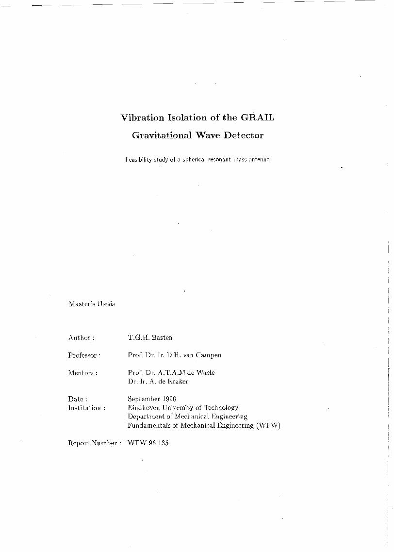
In the Netherlands a resonant mass detector is proposed which has been named GRAIL (Gravitational Radiation Antenna In Leiden). The basic design of the detector proposed by Frossati [lo], given in Figure 1.1, consists of a solid sphere with a diameter of 3 [ml and a weight of more than 100 tons with the resonant frequency of the lowest quadrupole modes between 650 and 750 Hz. Because the rate of detectable events in our own galaxy is too low the detector must also be capable to detect events out of our own galaxy. This implies tha t the sensitivity of the detector müst Se so high that vibrations of the sphere Zt these freqfiencies with an amplitude of lop2’ m can be detected. These are extremely small displacements and this requires that all vibrations due t o other sources than gravitational waves may not influence the measurement and therefore have t o be isolated. The main sources of noise are seismic and thermal vibrations. The first are isolated via a mechanical suspension. The thermal vibrations are reduced by cooling the sphere t o several mK.
Mechanical suspension
The proposed vibration isolation system of GRAIL consists of a room temperature level and a low temperature level. The room temperature part consists of an air bellow support and a stack of rubber and steel disks. The support rests on the ground while the rubber-steel stack holds the first low temperature stage. The low temperature level consists of three stages of two metal disks separated by helium bellows. The stages are separated from each other by means of metal rods. The last stage is connected t o the centre of the sphere by means of a copper rod. This is called a nodal suspension because the centre of the sphere is a nodal point of the five relevant quadrupole modes.
Cryogenics
The cryogenic part of GRAIL consists of a dilution refrigerator which holds the sphere on a temperature of 10 t o 50 mK. Around the sphere two shields are placed; the first at 50 mK, the second at 0.7 K. A vessel with liquid helium is placed around these shields. Then again two shields are placed; the third at 70 K and the fourth at room temperature. The difficulty of the cryogenic part is that it has to make good thermal contact with the sphere but poor mechanical contact. Therefore the shields and the helium vessel are suspended independently of the sphere.
2
Introduction 3
Rubber dampers for
Rubber damper for sph
Concrete support
Rubtoer damper €or helium vessel
filled bellows Dilution refrigerator
3 m Diameter
mK copper shield Copper rod suspens
ield
and thermal link \ 70 K shield
Figure 1.1: Design for GRAIL
Transducer
In order t o detect the extremely small vibrations of the sphere, they have t o be amplified by means of multi-mode transducers (not shown in the figure). These transducers are formed by coupled harmonic oscillators of decreasing mass. They have potentially a high sensitivity and a bandwidth approaching the resonance frequency of the antenna.
1.4 Research objectives
This thesis deals about vibration isolation of GRAIL and therefore mainly about the me- chanical suspension. This suspension contains a series of masses connected with springs and dampers. This cascade of isolation elements acts as a low pass filter for vibrations. The suspension must satisfy two main conditions:
o To prevent noise degradation by ambient noise, the antenna must be isolated as much as possible from the external environment.
o To achieve a reasonable signal to noise ratio the noise temperature of the sphere has to be low. This can be achieved by introducing very low damping in the sphere which
3

Introduction 4
means tha t the extrinsic quality factor of the antenna (that is, the quality-factor of the sphere loaded by the suspension and transducer and any other couplings) must be very high. A high &-factor means that the thermal vibrations of the sphere are minimized.
Secondary requirements for the vibration isolation system:
o It must be as simple and reliable as possible. It is not recommendable to design new things which could be difficult t o realize and which have a lot of uncertainties. I t wouid be better to design as robust as possible with proved teehniqües and with great reliability.
o The system has t o be easily accesible. If the antenna doesn't function properly the first time it is in operation the antenna has t o be easily dismantable and repairable.
The objective of this research is t o study the feasibility of the vibration isolation of GRAIL. The construction which is proposed by Frossati will be analysed and criticized where needed and optimized where possible. In chapter 2 the mechanical suspension will be analysed by means of simple linear models. In chapter 3 some continuous effects like wave propagation in metal rods and violin movements will be studied. In chapter 4 results of experiments on a simple small scale model will be compared with theoretical predictions. In chapter 5 other vibration souTees than seismic vibrations will be examined and finally in chapter 6 some conclusions and recommendations will be presented.
'The quality factor can be considered as inverse damping. For systems with low damping it can be approx- imated by W,/(WS - w ~ ) where w, is the resonant frequency and W I and wz are the half power points.
4

Chapter 2
Seismic vibrations
The natural and artificial sources of seismic noise are very numerous and varied., Natural sources are for example tectonic motions of the earth’s crust, storms, wind and water in motion. Examples of artificial sources are traffic, machinery, and general industrial activity. These noise sources combined produce a general continuous background of seismic motions which is termed seismic noise. One fairly consistent finding at reasonably quiet sites is that the linear spectral density of displacements in each direction varies to a good approximation as l/f2 [2], [15]. This corresponds t o a spectral density of acceleration independent of frequency.
If it is assumed that the linear spectral density of vertical seismic vibrations of the ground = l O W 5 / f 2 m/&
over the range 100 Hz t o IkHz, which is a very pessimistic assumption [a], then the linear autopowerspectrum of vertical seismic vibrations of the ground at 700 Hz has a magnitude of 2.0 . m/&. The autopowerspectrum of the vibrations of the sphere Jssp can be predicted then by means of the transfer function H ( f ) (see Appendix H).
at the place where the detector may be built is given by
The objective is t o detect vibrations of the sphere with an amplitude less than 5 . m. This implies tha t the amplitude of the transferred vibrations has t o be reduced with more than 215 dB. The objective of the vibration isolation system is t o achieve an isolation of more than 350 dB, which is more than sufficient for seismic vibrations. This attenuation seems t o be possible t o realize as will be shown. The detector may be built in Amsterdam. The real seismic vibrations there will be measured by KNMI (Koninklijk Nederlands Meteorologisch Instituut).
2.1 Modelling the mechanical suspension system
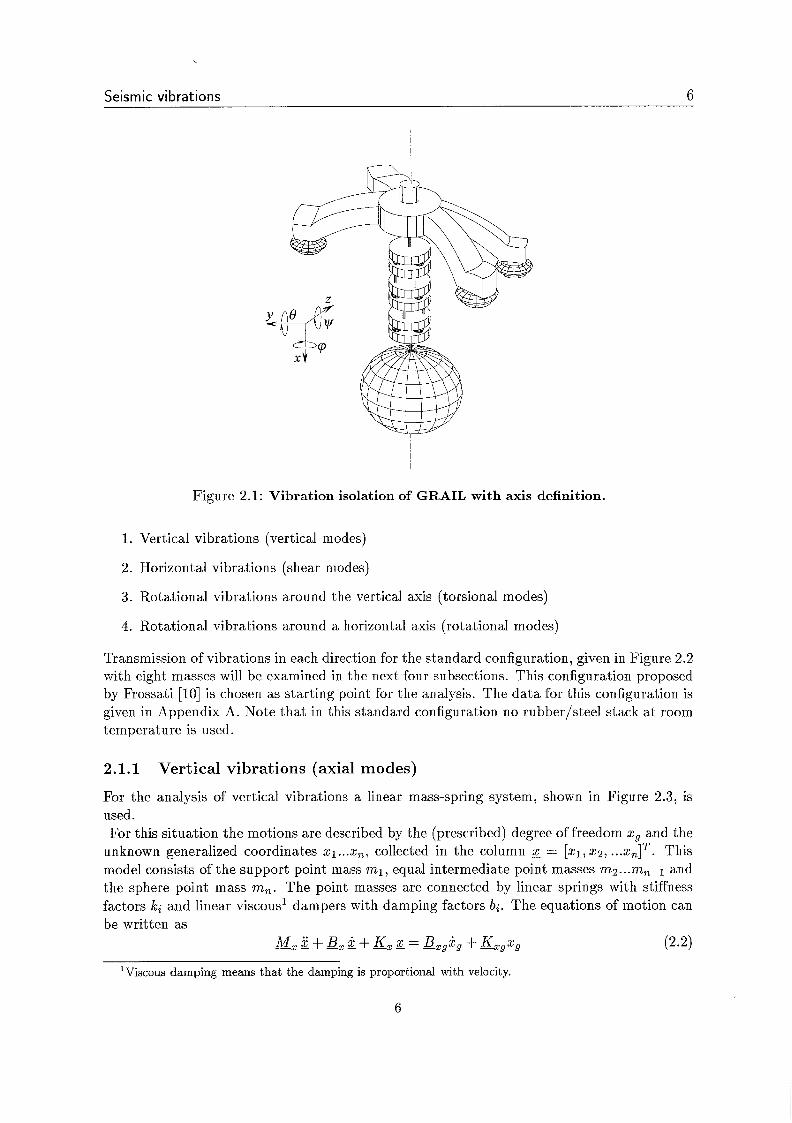
In Figure 2.1 the mechanical suspension of the sphere, the sphere itself, and a coordinate definition is given.
Vibrations along the three directions, given in the figure and vibrations around the three axes will be examined. It is assumed that all the displacements and rotations are very small so that a linear theory can be applied. The sources of vibration are the vibrations of the ground. Due to symmetry around the vertical axis four different linear equations of motion remain:
Seismic vi brat ions 6
Figure 2.1: Vibration isolation of GRAIL with axis definition.
1. Vertical vibrations (vertical modes)
2. Horizontal vibrations (shear modes)
3. Rotational vibrations around the vertical axis (torsional modes)
4. Rotational vibrations around a horizontal axis (rotational modes)
Transmission of vibrations in each direction for the standard configuration, given in Figure 2.2 with eight masses will be examined in the next four subsections. This configuration proposed by Frossati [lo] is chosen as starting point for the analysis. The da ta for this configuration is given in Appendix A. Note that in this standard configuration no rubber/steel stack at room temperature is used.
2.1.1 Vertical vibrations (axial modes)
For the analysis of vertical vibrations a linear mass-spring system, shown in Figure 2.3, is used. For this situation the motions are described by the (prescribed) degree of freedom 2, and the
unknown generalized coordinates 2 1 ... x,, collected in the column 2 = [XI, 22, ... z,lT. This model consists of the support point mass ml, equal intermediate point masses m2 ...mn-l and the sphere point mass m,. The point masses are connected by linear springs with stiffness factors k; and linear viscous1 dampers with damping factors b;. The equations of motion can be written as
J- M It. + B, + I& = &,i, + &,2, (2.21
'Viscous damping means that the damping is proportional with velocity.
6

Seismic vibrations 7
n
Air bellows I Concrete support /, /////ï
Titanium g d Helium bellows
Titanium rods
Helkm be!!ows
Titanium rods
Helium bellows
Copper rod o Copper disk Copper disk
CIpper disk Copper disk
Copper disk Copper disk
Sphere (CuA1)
Figure 2.2: Standard configuration with eight masses.
. . . . . . . .........................
x g , k l J + b , ,
n - i 4 X
n C
I . I . I . I .
Figure 2.3: Linear model for vertical vibrations.
7

Seismic vibrations 8
with &, B, and K , representing respectively the mass-, damping- and stiffness-matrices (see Appendix A). If a harmonic excitation z,(t) = Xgeiwt is assumed and consequently a harmonic response g( t ) = Xeiwt, the frequency response functions (frf’s) can be written as
X &(u) = = = ( - M , W 2 + B 3 s i W + $ - ) - l ( B 3 s g i W + ~ , ) . 2 (2.3) x,
The transfer function is a column in which element i represents the complex response of mass i t o harmonic movements of the ground. The nth element gives the complex response of the sphere. The absolute values of all frf’s and the damped eigenfrequencies for the standard configuration with eight masses (n=8) are given in Figure 2.4.
The essence of vibration isolation becomes visible now. For high frequencies the attenu- ation increases very fast with increasing frequency so for high frequencies the attenuation of vibrations is very high [6]. Each mass in the suspension has a substantial contribution t o this attenuation. The attenuation at the sphere at 700 Hz appears t o be 465 dB which meets the goal of 350 d B easily.
The assumption of viscous damping is made for the reason that with this type of damping an under estimation for the isolation in the system is obtained, which will be shown later. Another type of damping that could be used, called complex damping, is a type of damping which is frequency independent. This type of damping generates an upper estimation for the isolation because the real damping in the structure probably will be a combination of frequency dependent (connections, bellows) and frequency independent damping (rods). An under estimation for the isolation is always a save estimation.
2.1.2
For torsional vibrations around the vertical axis a similar linear model as for vertical vibrations is used, now with the prescribed rotation 4, and generalized coordinates - q5T = [41,42, ...&I (see appendix B). For the complex transfer function follows
Torsional vibrations around vertical axis (torsional modes)
The nth element of this column represents the complex response of the sphere to harmonic rotations of the ground around the vertical axis.
For the standard configuration the absolute value of the eight frf’s together with the damped eigenfrequencies are given in Figure 2.5. The attenuation at the sphere at 700 Hz is 641 dB.
2.1.3 Horizontal vibrations (shear modes)
Also for horizontal vibrations a similar linear model as for vertical vibrations can be used, now with the prescribed rotation y, and generalized coordinates - yT = [yi, y2, ...yn] (see appendix C). For the complex transfer function follows
2Analyses of these kind can easily be carried out by using the program MATLAB.
8

Seismic vibrations 9
. . . . . . . . . . . . . . . . . . . . . . . . . . . . . . . . . . . . . . . . . . . . . . . . . . . . . . . . . . . . . . . . . . . . . . . . . . . . . . . . . . . . . . . . . . . . . . . . . . . . . . . . . . . . . . . . . . . . . . . . . . . . . . . . . .
Figure 2 is given
. . . . . . . . . . . . . . . . . . . . . . . . . . . . . . . . . . . . . . . . . . . . . . . . . . . . . . . . . . . . . . . . . . . . . . . . . . . . . . . . . . . . . . . . . . . . . . . . . . . . . . . . . . . . . . . . . . . . . . . . . . . . . . . . . . . . . . . . . . . . . . . . . . . . . . . . . . . . . . . . .
'.4: by
-100
-2001
. . . . . . . . . . . . . . . . . . . . . . . . . . . . . . . . . . . . . . . . . . . . . . . . . . . . . . . . . . . . . . . . . . . . . . . . . . . . . . , . . . . . . . . . . . . . . . . . . . . . . . . . . . . . . . . . . . . . . . . . . . . . . . . . . . . . . . . . . . . . . . . . . . . . . \ : : : : : : : I . . . . . . . . . . . . . . . . . . . . . . . . . . . . . . . . . . . . . . . . . . . . . . . . . . . . . . . . . . . . . . . . . . . . . . . . .
. . . . . . . . . . . . . . . . . . . . . . . . . . . . . . . . . . . . . . . . . . . . . . . . . . . . . . . . . . . . . .
Transfer functions for vertical vibrations. The transfer function for (-1.
o p . I p,: . \ : . . . . . . . : . : : . : : )i 7 T YYS .\. 1 . . . . . . . -100 . . . . . . . . . . . . . . . . . . . . . . . . . .
1 O0
. . . . . . . . . - _ _ . . i > - . . . . . . ..... . . . . . . . ._ . . > . . .
-400 -300:
...
. . . . . . . . . . . . . . . . . . . . . . . . . . . . . . . . . . . . . . ......... . . . . . . . . . . . . . . .
. . . ........ . . . . . . . . ~
P - I i i ; . .
. . . . . . . . . . . . . . . . . . . . . . . . . . . . . . . . : : : : f8a 54.24 &: : : : : : : . . . . . . . . . . . . . . . . . . . . . . . . . . . . . . . . . .
-700
-800 1 O-' 1 oo 1 O' 1 o2 i o3 1 o4
Frequency [Hz]
the sphere
Figure 2.5: Transfer function for torsional vibrations around the vertical axis. The trans- fer function for the sphere is given by (-).
9

Seismic vibrations 10
For the standard configuration the absolute value of the frf’s together with the damped eigenfrequencies are given in Figure 2.6. The attenuation at the sphere at 700 Hz appears t o be 634 dB.
2.1.4
The final linear model is the one for rotational vibrations around a horizontal axis with prescribed rotation yg and generalized coordinates QT = [O,, 02, ... O,] (see appendix D). For the compiex transfer function foiiows
Rotational vibrations around a horizontal axis (rotational modes)
For the standard configuration the absolute value of the transfer functions together with the damped eigenfrequencies is given in Figure 2.7. The attenuation at 700 Hz is 556 dB.
For the given model it is assumed that each mass rotates around its center of mass. In practice the masses are not suspended exactly in the centers of mass so a gravitational effect plays a role and can even make the suspension unstable. In Figure 2.8 such an unstable suspension is given.
Obviously this suspension is unstable but i t is proven here also mathematically. Rotations of the f i rs t ifitermediate mass (mz), which is comected with the support, around its center of mass are examined and the effect of gravitational forces for the stability of this structure is considered. It is assumed that the points indicated by a solid dot are free rotation points and that connections itself have no contributions in the potential energy. The potential energy of the standard system with eight masses when gravitational forces are included is written by
v = m2g(hcos02)
+ m3g(3hcos& + b) + + + + +
m4g(5hcosQ2 + b - 1 2 )
m5g(7hcosQ2 + 2b - Za) m~g(9hcoso2 + 2b - z2 - Z3)
m7g(llhcos02 + 3b - z2 - Z3)
msg(l2hcosez + 3b - 12 - z3 - Z4)
The derivative of the potential energy t o the angle OZ is
= - h ( m ~ + 3m3 + 5m4 + 7m5 + 9mG + í1m7 + 12ms) sin 02. (2.8) i3V 802 -
So for small deviations of 192 around the state of equilibrium 02 = O the potential energy decreases (i3V/6’02 < O) what means that this system is unstable.
The real system must be stable so care has t o be taken t o avoid instability. Three possible solutions t o solve this problem are given here. The first one is t o position the connection points below the centers of mass of the attaching masses. The consequence of this solution is that the suspension loses its compactness. The second solution is t o increase the contact areas between the suspension points and the masses. The final and best solution is t o suspend the first intermediate mass (mass m2) by three parallel rods instead of the present single rod.
10

Seismic vibrations 11
-200 I
Frequency [Hz]
-500 ' 1 . . . .
. .
. . . .
Figure 2.6: Transfer function for horizontal vibrations. The transfer function for the sphere is given by (-).
-200 -
-300 -
-400 -
-700
-800 1 o4 1 O-* 1 O-' 1 oo 1 O' 1 o2
Frequency [Hz] 1 o3 1 o4
Figure 2.7: Transfer function for rotational vibrations around y- or z axis. The transfer function for the sphere is given by (-).
11

Seismic vibrations 12
2 9
arn. e = Centre of mass
Figure 2.8: Schematic view of an unstable suspension.
2.2 Model parameters and vibration isolation
In the previous section i t is shown that vertical vibrations along the vertical axis appear the most difficult ones t o attenuate. Therefore, in this section only the transfer function of the sphere for vertical vibrations (Equation 2.2) is examined in more detail. The transfer function can be subdivided in four parts (see Figure 2.4). For very low frequen- cies the amplitude of the vibration of the sphere equals the amplitude of the vibrations of the ground ( H z ( f ) = 1). For low frequencies a number of resonance peaks equal t o the number of masses in the model appear at each resonant frequency. For medium and high frequencies the transfer function can be approximated by simple func- tions (see Appendix A). For medium frequencies the absolute value can be approximated by
and for high frequencies by
(2.10)
These functions are given in Figure 2.9. So with viscous damping the isolation increases with f " for high frequencies and for the
medium frequency range it increases with f 2 " . The width of this range is determined by the coefficients ki and b;. The lower the ratios b i / k i , the wider Ihis frequency range. From the approximations for medium and high frequencies the next conclusions can be drawn:
12

Seismic vibrations 13
Frequency [Hz]
Figure 2.9: Frequency response function with approximations for medium (. .) and high (---) frequencies.
The number of masses in the vibration isolation system determines the gradient of the frequency response functions. Applying more masses in the system results in a steeper frequency response function for high frequencies.
The stiffness and damping factors together with the masses determine the height of the asymptotes. Low stiffness and damping factors and heavy masses improve the vibration isolation. From this point of view the statement can be made that it is better t o use intermediate masses with the same weight. For example three intermediate masses of 5000 kg each give better results than three masses of respectively 1000, 5000 and 9000 kg ’. This statement is valid for isolation of seismic vibrations. It is uncertain whether equal intermediate masses give also maximum isolation of thermal vibrations.
The role of damping is ambiguous. On one hand it lowers the resonance peaks. On the other hand, with damping, high-frequency ground motions are easier transmitted than without damping. This conclusion holds for viscous damping. If complex damping is used the response function is given by
(2.11)
where &. and Kzg,c are complex stiffness-matrices. The elements are formed by the complex stiffness coefficients: k,,; = k;(1+ j & ) . For medium and high frequencies the absolute value can now be be approximated by Equation 2.9. So for medium frequen- cies it doesn’t matter if complex or viscous damping is used in the model. For high frequencies the model with viscous damping gives an under estimation for the isolation. Complex damping on the other hand gives an upper estimation.
30ptimizing the function g = nr=l mi with the constriction Er=, mi = M gives mi = M / n .
13

Seismic vibrations 14
2.3 Alt ernat ive configurations
The influence of the number of masses, the values of the masses and the stiffness- and damping factors on the vibration isolation has become clear now. With this information it is possible t o compose different configurations which meet the requirement of vibration attenuation at 700 Hz with more than 350 dB.
The objective of this section is to find different appropriate configurations which are as simple as possible. Especially the role of the helium dampers and the addition of rubber and steel disks in the Toom tempera txe part of the suspension is considered.
In Table 2.1 the attenuation at 700 Hz is given for various configurations, together with the highest eigenfrequency. The number of low temperature stages is varied by doing calculations for one, two and three low temperature stages4. The number of room temperature stages are varied by introducing a stack of rubber and steel elements. The position of these elements in the structure is drawn in Figure 2.10. All configurations are considered with and without
- Steel disk .,
Figure 2.10: Position of rubber/steel stack in the structure.
helium dampers. In the latter case the eight helium dampers per stage are replaced by three titanium rods of 1.5 m in parallel. The material, which is used for the rubber disks, is neoprene which is creep-proof, attaches good to metals and has good damping properties. The steel masses have a weight of 500 kg.
40ne low temperature stage consists of two intermediate masses separated by helium bellows.
14

Seismic vibrations 15
2 -322 165.1 -316 3 -350 184.7 -346
Table 2.1: Attenuation values for suspensions with and without helium dampers together with the highest damped eigenfrequency of the systems. r is the number of rubber/steel stages in the stack, while s represents the number of low temperature stages.
i 6 5 2 176.0
2 3
1 He-dampers I Ti-rods I
-427 165.1 -414 165.2 -461 175.9 -447 176.0
s=2
2 3
I
-532 165.1 -512 165.2 -565 175.9 -546 175.9
I
I 1 I -498 I 135.9 1-479 I 136.0 1 S=Y I I I I
From these results it becomes clear that for vibration isolation it is not absolute necessary t o use helium dampers because the differences in stiffness coefficients of titanium rods and helium dampers is insignificant. The question arises if the advantages, which are compactness and the possibility t o adjust the resonant frequencies, can counterweight the disadvantages. These disadvantages are many internal modes with frequencies which are hard to predict, the possibility of leakage, unknown dissipation and a lack of practical experience with helium dampers.
If the isolation system is well-analyzed no resonances will appear at the antenna-frequency and the suspension can be built rather compact even by using rods only.
The most efficient configuration appears to be a room temperature part and a two-stage low-temperature part. The room temperature part attenuates most seismic vibrations while the low-temperature part attenuates the thermal vibrations of the high temperature part and gives a high extrinsic quality factor5 for the vibrations of the sphere. Whether this configuration is also sufficient t o attenuate thermal vibrations sufficiently has to be studied.
5The quality factor of most materials increases with low temperature.
15
Seismic vibrations 16
2.4 Quality factor
To achieve a noise temperature T N ~ , the extrinsic quality factor of the antenna must satisfy Q > (TU/T~)wuq, where Ta is the thermodynamic temperature, w, is the frequency of the fundamental resonant mode of the sphere and r; is the optimum integration time for the system. A high &-factor means that the thermal vibrations in the sphere are minimized. To obtain a reasonable &-factor the sphere is suspended in the centre. This is a nodal point of the fundamental resonance modes of the sphere. In theory these modes are therefore not excited by the siispension SO the extrinsic &-factor wil! be hardly &tubed . This nodal siispensim, however, will never be perfect because of a certain contact area. Yet, the extrinsic &-factor will still be high because the lower suspension stages are made of high Q materials. The influence of the suspension on the extrinsic &-factor has to be studied in detail or measured in practice.
2.5 Upconversion
Up t o now only high frequency mechanical vibrations were concerned about because the rele- vant gravitational wave signals are of high frequency. However, the low frequency vibrations with much larger amplitudes must not be forgotten. The low frequency noise always can ex- cite non-linear processes like stick-slip in sliding contacts, which can lead t o strong excitation at the antenna frequency. For this reason two remarks can be made:
a
a
2.6
Sliding contacts must be avoided. Therefore solid rods have t o be applied instead of cables and i t would be better not t o bolt these rods t o the metal disks but to weld them. This has consequences for the materials which can be used.
The largest low-frequency vibrations appear at the resonant frequencies. The amplitudes of vibrations of the sphere can be very high there. They can even be higher than those of the moving ground. It would therefore be better t o lower the resonance peaks.
Active control of low-frequency vibrations
Possible methods to reduce the resonance peaks are raising the damping in the system or using active control [l]. By raising the damping coefficient, the peak heights are lowered. A result of this action, however, is that the attenuation at higher frequencies is worse. An example is given in Figure 2.11 where the frequency response is given for the structure with
ten times higher (& = 0.3). The peaks are lowered considerably by raising the damping but the attenuation at 700 Hz has been worsened by 20 dB. This is not very much so raising the damping of the first room temperature stage is a useful possibility t o lower the peaks.
Another method t o lower the low-frequency resonance peaks, without affecting the at- tenuation at high frequencies, uses active control. The model for vertical vibrations with a control mechanism which uses the PD control strategy [8] (see Appendix E) is considered here.
In Figure 2.12 the first mass is suspended via a spring and a damper. The controller R determines the control force F which should be applied t o the mass as a result of the
= 0.03 and with
‘The noise temperature is defined as TN = AE,/kB where AE, are the energy fluctuations due to noise.
16

Seismic vibrations 17
displacement and velocity characteristics of the mass. This force is calculated using the relation
F ( t ) = K((2dl - .1) + Q(&l - 21))- (2.12)
The purpose of attaching an active element to the system is to fix the mass in a certain position (i.e. the desired position). This requirement means tha t
2&) = o ; i&) = o. (2.13)
Introducing condition (2.13) in Equation (2.12) yields
F ( t ) = -Kx,(t) - I'h&-il(t). (2.14)
Now the equation of motion of the first mass is
mizi + (b i + b2 + 1 ( ~ d ) i 1 + (hl + .F2 + l i ' )~ i = b 2 2 2 + IC222 + bi2 , + I C ~ X , , (2.15)
and the system is described with the matrix equation (see Appendix E)
M - a + + & = &,li., + &,x,. (2.16)
For the transfer function Hg = &'Xg follows
x H - =(u) = (-&u2 + g i w + K;)-l - (&,u + Lg). (2.17)
- x, In Figure 2.13 the transfer function for the controlled system with K = 1.0. lo8 N/m and rd = 0.1 s is shown, together with the transfer function for the uncontrolled system. It is
17

Seismic vibrations 18
x 1
x 2
3 X
X
Figure 2.12: Multiple degree of freedom control system.
Figure 2.13: Response function without (--) and with (-) active damping.
18

Seismic vibrations 19
clear that by using active control the results at low frequencies are considerably better than without control without having affected the attenuation at high frequencies. If this result is compared with the transfer function with increased damping (Figure 2.11), then i t is clear that the peaks with active control have been lowered even more than with increased damping.
An example of an occurrence is given in Figure 2.14. The ground suddenly begins t o move sinusoidal on t = 1 with a frequency of 1.5 Hz and an amplitude of 1 . loM5 m. In Figure 2.14a the response of the sphere is given for the uncontrolled situation and for the controlled
Figure 2.14b the control force is given. --L.--+:-- ,,,:CL v - i n ln8 RT lm u;liudilil"II W l b l l 11 - I." I" L Y , 111 2Ed 7-d = 0.1 tegether with the rri^vement G f the grnlind. In
Time [SI
~
Time [SI
Figure 2.14: a) Time simulation for the movement of the sphere for the controlled (-) and uncontrolled system (--) together with the moving ground (. ..). b) Control force.
It can be concluded now that lowering the peaks at low frequencies is not possible with passive solutions without losing performance in the attenuation a t high frequencies. A possible solution is t o make use of PD control. A simple model of the controlled structure is considered t o examine the effect of active isolation. The preliminary results are satisfying. Further calculations and model refinement is necessary before drawing hard conclusions with respect t o the potential and need for active vibration control in this structure. Among items of further investigations is the study of actuator dynamics and the technical possibility t o induce such high control forces.
19

Seismic vibrations 20
2.7 Discussion
From the examined vibrations longitudinal ones are most difficult t o isolate but it seems to be possible t o attenuate seismic vibrations at 700 Hz with more than 350 dB.
It may even not be necessary t o use helium dampers. The advantages of these dampers are compactness and possibility to adjust the resonance frequency but they don’t counter- balance the uncertainties of these bellows. Although a simple analysis has shown that the bellows are stable (see Appendix F) the functioning of these bellows in practice under ex- treme circumstances is very Uncertain. A constriiction with only rneta! rods connecting the intermediate masses already meets the requirements and, if well-analysed, no resonance peeks will be harmful.
It is demonstrated that active control gives better attenuation of low frequency vibrations. However, the remaining question is how active control can be applied in practice for both horizontal and vertical vibrations.
20
Chapter 3
Continuous systems
In the previous chapter the mechanical suspension, which in fact consists of continuous el- ements, was described by mass-spring-damper models. The connections were considered to be mass-less and point masses were used for the support, intermediate disks and the sphere. In this chapter some effects which can’t be described with these models will be examined by modelling the suspension as a continuous system and by modelling the bodies as having distributed mass.
In the first section wave propagation in metal rods is examined. In the second section a continuous model for transverse vibrations of metal rods is set up. The third section handles about the eigenfrequencies of the intermediate masses. The investigation of the internal modes of the helium- and air bellows is beyond the scope of this thesis.
3.1 Wave propagation in metal rods
In the previous chapter the rods in the model for vertical vibrations were considered as linear mass-less springs. In fact these metal rods are continuous systems in which elastic waves can propagate. In this section this effect is examined for a single rod where the partial differential equation for vertical vibrations is solved analytically. This analytic solution is compared with the results for a discrete mass model of the rod. After that , a discrete mass model is set up for the GRAIL vibration isolation system of which the transfer functions is compared with the transfer functions calculated for the mass-spring-damper model of the previous chapter.
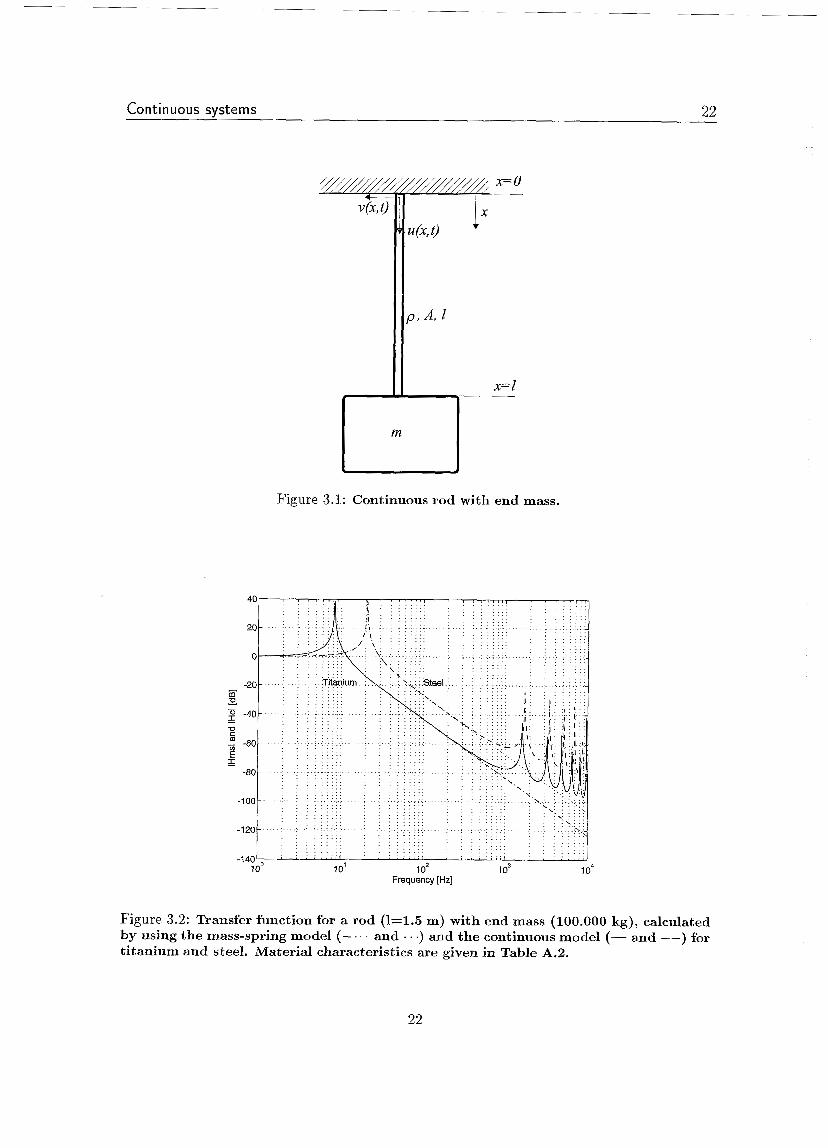
In Figure 3.1 a single rod is given which is connected with an end mass. For longitudinal vibrations of this rod the following transfer function is valid (see Appendix G )
4 4 t ) - E A - H ---
- ~ ( o , t ) E A cos $ - mew sin e Where E is the Young’s modulus, 1 the rod length, A the rod cross section area determined by the maximum axial stress o,,, and safety-factor a. The wave constant is calculated by c = m. The resonance frequencies wn can be calculated from
Uni wnl E A cos - - mew, sin - = O. c e
In Figure 3.2 the transfer functions for both the mass spring model and the continuous model for respectively steel and titanium are given.
21
22 Con t i n uous systems
Figure 3.1: Continuous rod with end mass.
.- Frequency [Hz]
Figure 3.2: Transfer function for a rod (1=1.5 m) with end mass (íOO.000 kg), calculated by using the mass-spring model (- . - and . . .) and the continuous model (- and --) for titanium and steel. Material characteristics are given in Table A.2.
22

Conti n uo u s systems 23
It is clear tha t for low frequencies the two models give the same transfer of vibrations. For frequencies higher than approximately 500 Hz the differences between the transfer functions get wider. Obviously for high frequencies the rod cannot be modelled as a linear spring,
3.1.1 Optimization of rod length
It is possible to maximize the isolation for vibrations with a certain frequency by optimizing the rod length [5], [18]. The transfer of vibrations at a certain antenna-frequency w, as a ftinction of the rod leiìgth is given for the cofitinuous rod model by
E A E A cos % - mew, sin % Hc(1) =
and by Equation 3.4 for the mass spring model
E A E A - mlwa a n s ( q =
(3.3)
(3.4)
In Figure 3.3 the transmission of vibrations at 700 Hz as a function of the rod length for both the continuous model as the mass-spring model for steel and titanium is given.
Length rod [m]
Figure 3.3: Transfer of vibrations of 700 Hz as a function of the rod length, calculated by making use of the linear model (- . - and . . .) and the continuous model (- and --) for titanium and steel.
From these figures i t can be concluded that the vibration isolation has a maximum at a certain rod length. This optimum length can be calculated with
d f f c -(I = Iopt) = o. dl (3-5)
For steel follows Zopt = 1.85 m and for titanium lopt = 1.73 m.
23

Continuous systems 24
The vibration isolation of titanium rods for the given rod length is much higher than that for steel rods (74.4 dB for titanium and 58.9 dB for steel) due to a higher tensile strength and a lower Young’s modulus. To achieve a maximum vibration isolation titanium is therefore much better than steel.
3.1.2 Discrete rod model
In this chapter a transfer fmction for a continiioiis rod with an end mass in anaiyticaÏ form has been derived. The vibration isolation system of GRAIL consists of a cascade of masses and rods. Deriving an analytic expression for the transfer function for the total system is very difficult and it would be useful if an approximation for a certain frequency range could be generated. This is possible by making use of a discrete mass model. First such a model will be derived for one rod with one end mass and then a model for the mechanical suspension of GRAIL is derived.
The basic concept of the discrete mass model is to model the rod which has a finite mass as a chain of masses and springs (see figure 3.4).
Figure 3.4: Lumped mass model for a continuous rod with end mass.
The total mass of the discrete masses equals the mass of the rod, so ml = pAZ/n where p is the material density, A the rod cross section area, 1 the length of the rod and n the number of discrete masses. The total stiffness equals the stiffness of the rod ( k = nEA/E). The results for this model with various numbers of discrete masses together with the continuous model are given in Figure 3.5.
I t is shown that the more discrete masses are used, the wider the frequency range for which the approximation follows the transfer function of the continuous model. Taking into account these results, the assumption arose that the vibration isolation system of GRAIL can be modelled with a discrete mass model. The results of this analysis together with the results found in chapter 2 are given in Figure 3.6.
It is clear tha t for high frequencies wave propagation plays a modest role in the vibration isolation and tha t internal resonance peaks near the antenna frequency must be avoided.
24

Continuous systems 25
Frequency [Hz]
Figure 3.5: Transfer functions for discrete mass models with 2(. ..), 4(- . -) and S(--) discrete masses together with the transfer function for the continuous model (-).
. . . . . . . . . . . . . . . .
. . . . . . . . . . . . . . . . . . . . . . . . . .
. .
. . . .
. . . . . . . .
. . E-200b . :: -; . . . . . . . . . . -
...
. . . . . . . . . . . . . . . . . . . . . . . . . .
. . . . . . . . . . . . . . . . . . . . . . . . . . . .
. . . . . . . . . . . . . . . . . . . . . . . . . . . . . . . . . .
. . . . . . . . . . . . . . . . . . . . . . . . . . . . . . . . . . . . . . . . . .:.
. . . .
Frequency [Hzj
Figure 3.6: Results of the lumped mass model of vibration isolation system of GRAIL (- - -) together with the results for the mass-spring-damper model of chapter 2 (--).
25
Continuous svstems 26
3.2 Transverse vibrations
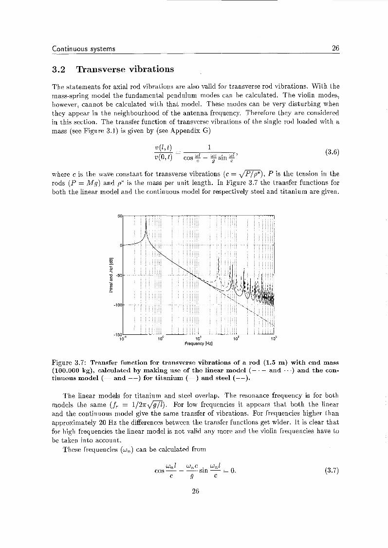
The statements for axial rod vibrations are also valid for transverse rod vibrations. With the mass-spring model the fundamental pendulum modes can be calculated. The violin modes, however, cannot be calculated with that model. These modes can be very disturbing when they appear in the neighbourhood of the antenna frequency. Therefore they are considered in this section. The transfer function of transverse vibrations of the single rod loaded with a mass (see Figure 3.1) is given by (see Appendix G)
where c is the wave constant for transverse vibrations (c = m), P is the tension in the rods ( P = M g ) and p* is the mass per unit length. In Figure 3.7 the transfer functions for both the linear model and the continuous model for respectively steel and titanium are given.
1 oo 1 o’ 1 o2 1 o3 Frequency [Hz]
Figure 3.7: Transfer function for transverse vibrations of a rod (1.5 m) with end mass (iOO.000 kg), calculated by making use of the linear model (- . - and .. .) and the con- tinuous model (- and --) for titanium (-) and steel (--).
The linear models for titanium and steel overlap. The resonance frequency is for both models the same (fT = 1/2nJsTt>. For low frequencies i t appears that both the linear and the continuous model give the same transfer of vibrations. For frequencies higher than approximately 20 Hz the differences between the transfer functions get wider. I t is clear that for high frequencies the linear model is not valid any more and the violin frequencies have to be taken into account.
These frequencies (un) can be calculated from
wnl wnc . wnl cos - - -sin - = O.
C g C (3 .7)
26

Conti n uous svste ms 27
The first pendulum frequency (n=O) is approximated by WO N wp = &$. The resonance frequencies of the violin modes of the rod are approximated by
where m, is the mass of the rod. To reduce the effects of violin modes the resonance frequencies should be as high as
possible. Therefore, rods of low mass density and high tensile strength like titanium are desirable [13].
If tubes are used instead of massive rods the string-theory which is applied here is not valid any more and the beam-theory has to be applied. Using the beam-theory it can be shown that the resonance frequencies of the violin modes can be influenced by adjusting the polar moment of inertia. However, this is not investigated in this thesis.
3.3 Eigenfrequencies of the intermediate masses
In the models used so far the intermediate disks were considered as point masses which are infinitely rigid. However, internal modes of these disks affect the vibration isolation when their resonance frequencies are in the neighbourhood of the antenna-frequency. Therefore considering them as point masses is only valid when the resonance frequencies of the single masses are much higher than the antenna-frequency. Because of the negative influence of the internal modes it would better to avoid these resonance-frequencies near the antenna- frequency. In this section the resonance frequencies of the circular intermediate masses are calculated.
The eigenfrequencies of thin circular disks can be calculated by [3]
(3.9)
where r is the radius of the disk, h is the height, y is the mass per square meter (y = m/m2 = ph), E is the Young’s modulus and Y the Poisson’s ratio, A;j is a parameter which depends on the edge conditions and mode shapes ( i = number of nodal diameters, j = number of nodal circles). The lowest resonance frequencies are calculated for free circular disks and presented in Table 3.1. Though Equation 3.9 is not completely valid for the relative thick circular copper disks used in the proposed design (m N 5000 kg, h = 0.3 m + r = 0.77 m) fairly good approximations for the lowest frequencies of these disks are obtained.
For thick circular disks, with various boundary conditions, a numerical method t o calculate the resonance frequencies has t o be applied which is e.g. using a finite element program like MARC.
The lowest eigenfrequencies of three free circular copper masses with various dimensions are calculated by making use of the dynamic modal routine in MARC. Each mass is modelled with 90 elements as shown in Figure 3.8. The results are given in Table 3.2.
For thick circular disks, beside bending modes also modes with deformations in the plane of the disk have been calculated. These eigenfrequencies cannot be calculated by formula 3.9. Therefore finite element calculations are necessary. The eigenfrequencies of free circular disks which are considered in this chapter are very near the antenna frequency. For disks
27

Continuous systems 28
30 11
Table 3.1: Lowest eigenfrequencies of a free circular copper disk. Material characteristics are given in Table A.2.
1131 1898
Figure 3.8: Mesh for modal analysis of circular disks consisting out of 90 20-noded ele- ments.
with a high diameter-thickness ratio these frequencies are lower than for disks with a high ratio. Therefore it would be better to use disks with a high diameter-thickness ratio in the structure.
28

Conti n uous svst ems 29
20 o1 30 11
in plane in plane
~
Table 3.2: Lowest eigenfrequencies of a free circular copper disks with various dimensions. h is the thickness, while d is the diameter of the disk.
433.9 681.7 697.9 728.1 1107.1 866.3 906.4 1321.8 1189.7 1383.7 > 1600 > 1600 1120.6 1291.5 973.7 1319.6 1519.1 1214.4
3.4 Conclusions
For high frequencies the rods in the mechanical suspension cannot be modelled as linear springs because these springs don’t take into account axial and transverse dynamic behaviour of the rods. For longitudinal vibrations it is better t o model the rods with discrete mass models. These models give good similarities with continuous models. With a specific rod an optimum length for vibration isolation at a certain antenna-frequency can be computed. For titanium this length (1.73m) is a bit shorter than for steel (1.85 m). In general titanium rods give better vibration isolation than steel rods. Violin modes play an important role in the neighbourhood of the antenna-frequency. To make them as high as possible a material with low density and high tensile strength like titanium is preferred. With tubes the resonance frequencies of the violin modes can be adjusted. This possibility will be considered in further investigations. To avoid eigenfrequencies of the intermediate disks in the neighbourhood of the antenna- frequency the diameter-thickness ratio of these disks should be as high as possible. To make the analysis complete also helium and air bellows and the concrete support have t o be taken into account. This will also be a subject for further investigation.
29

Continuous systems 30
30

Chapter 4
Experiments
To check whether the theoretical predictions are valid for a real vibration isolation system and t o learn something about the practical problems of a vibration isolation system some small scale experiments have been carried out by Ad Hendrikx and Ton van Haren [9]. In this chapter the experimental setup is shown and the experimental results are compared with the theoretical predictions. Finally the differences are discussed.
4.1 Experimental setup
The main objective is to realize a setup which is simple but has great similarities with the mechanical suspension of GRAIL. The resulting setup is a device made of a large cylindrical
I
Shaker
Base-plate Metal Bellows 1 Steel wire
Disk (3.35 kg)
3 Steel wires
Disk (3.35 kg)
1 Steel wire
Cylinder ( 1 5.8 8 kg)
= Accelerometer
Figure 4.1: Experimental setup
31

Experiments 32
mass of 15.88 kg representing the sphere and two circular disks of 3.35 kg as intermediate masses. The masses, which are all made of brass, are connected with 0.7 mm thick diameter steel wires (see Figure 4.1). The setup can easily be dismantled. Therefore it is possible to do experiments with three, two and only one mass. A correction t o the original design was necessary t o make the suspension stable. In the original design the center of mass of the first disk was situated above the suspension point. This makes this design unstable. The problem is solved by making a hole in the disk so that the suspension point is moved t o a point above the center of mass, see Figure 4.2.
Stable
Figure 4.2: Unstable and stable suspension of the first disk.
The incoming vibrations are induced by means of a shaker. This shaker can induce vi- brations with different spectral composition such as white noise, periodic chirps, and sine sweeps. The shaker is placed on a thin base-plate of brass with which the first wire is con- nected. This plate is placed on metal bellows which stand on the ground. The displacements of the base-plate serve as the dynamic input for the suspension system.
The accelerations of each mass and of the base-plate are measured by means of accelerom- eters [14]. These small and very sensitive instruments have a large measuring range, up t o several kHz. For very low frequencies ( < l o Hz) they are unsuitable. The data is sent t o a computer where the transfer functions are calculated by the DIFA measuring system. These transfer functions are calculated from the measured autopowerspectra and cross-powerspectra (see Appendix H).
The transfer functions for the accelerations of the masses are the same as the transfer functions for the displacements. So there is no need to calculate the displacements first in order t o determine the transfer functions. For more details see [9].
4.2 Results
Simple mass-spring models as discussed in Chapter 2 have been set up for the vertical vibra- tions of the system with respectively one, two and three masses attached to the base-plate. The transfer function of the system with one mass for vertical vibrations from the base-plate to the mass is given by Equation 4.2.
32

Experi men t s 33
The transfer functions of the system with two masses of vertical vibrations from the base- plate t o the masses are given by
and for the system with three masses by
-1 O bi + b2 4 2 0 -1 f J c 2 4 2 o
- - X - - (- [ m2 O ] w 2 + [ -b2 b2+b3 -b3 io+
xbp 0 m 3 O 4 3 b3
bi +b2 -b2
-k3 Jc3
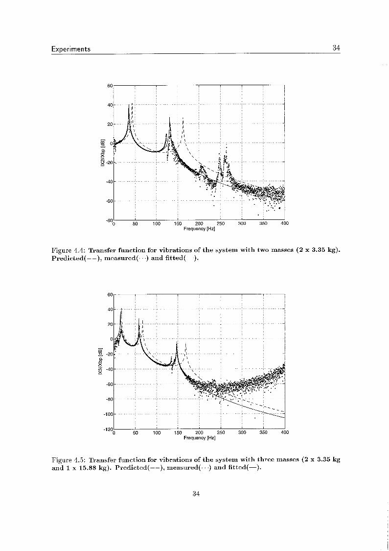
The predictions for the transfer function of vibrations of the shaker t o vibrations of the lowest mass together with the rneasiired transfer fiiiictions and the fitted transfer fEnctions to the measured ones are shown in respectively Figure 4.3, 4.4 and 4.5.
i 1
100 150 200 250 300 350 1
Frequency [Hz] O
Figure 4.3: Transfer function for vertical vibrations of the system with one mass (3.35 kg). Predicted(--), measured(. . .) and fitted(-).
For low frequencies (< 10 Hz) the accuracy of the accelerometers is very poor. Therefore the measured transfer functions for low frequencies cannot be compared with the theoretical curves.
33
ExDe r i men t s 34
j . . .
. . . . .. . . .< . .
a :
I 4 I I I I I
50 100 150 200 250 300 350 Frequency [Hz]
-80;
Figure 4.4: Transfer function for vibrations of the system with two masses (2 x 3.35 kg). Predicted(--), measured(. . .) and fitted(-).
I I I I I I I -1 20;
Frequency [Hz]
Figure 4.5: Transfer function for vibrations of the system with three masses (2 x 3.35 kg and 1 x 15.88 kg). Predicted(--), measured(...) and fitted(-).

Experi men t s 35
The differences in the positions of the normal mode resonances between the predicted transfer functions and the measured transfer functions can be explained by the differences in the theoretical and practical stiffness factors of the wires. The stiffness factors for the predicted curve are calculated by k = EA/Z. Actually these factors are about 30 % lower due t o the additional, unmodelled serial stiffness of the element which attaches the wires t o the masses. The fitted theoretical transfer functions are calculated by using these lower stiffness factors.
The damping in the wires is determined experimentally by looking t o the decrease of amplitudes of free damped vibrations. The dimensionless damping factor equals
Beside the resonance peaks due t o the normal modes of the system some other peaks can be noticed in the experimental transfer function. Some of these peaks can be explained by transverse resonance of the wires (violin modes). The resonance frequencies for the violin modes are calculated by
N U.01.
where mt is the total mass hanging on the considered wire, m, is the mass of that wire, and wp is the pendulum frequency (wp = m).
The first violin fîeqüency for the wire loaded with one mass calculated in this way gives a resonance frequency of 346.5 Hz. This is very close to the largest peak in the experimental transfer function for this system. This peak disappears when the wire is clamped in the middle.
The first resonance frequencies for longitudinal vibrations are calculated from
wnl WnZ E A cos - - mew, sin - = O c c (4.4)
Solving this equation numerically, 63.6 Hz is found for the normal mode and 17181.5 Hz for the first internal mode. The normal mode is clearly visible in the transfer function. The internal mode is not visible because the transfer function cannot be measured at high frequencies.
The measured transfer functions don’t follow the predicted ones because the energy of the high-frequency acceleration signals is too low. The reason for the low energy of the source signal at the base-plate is that near the cut down frequency the signal energy is lower than in the rest of the frequency range.
The reason for the low energy of the acceleration signal of the lowest mass is that the energy of the high frequency components decrease, due t o the low pass filter, beneath the noise level of the measuring system. Measuring the transfer function over a large frequency range in one run is therefore not a good strategy. As the energy of all frequency components of the source signal is equal, at low frequencies the system begins t o resonate while at high frequencies nothing can be measured a t the output. By using a source signal with only high- frequency components it is possible to increase the energy without bringing the system in resonance. In this way a better result for the measured transfer function is available. This has been done for the system with one mass and for the system with three masses. The transfer functions are measured in two runs. First for the low-frequency region and after that , for the high-frequency region. The results are given in Figure 4.6 and 4.7. Note that the transfer function for the one-mass system is measured with the wire clamped in the middle so no violin resonances appear.
35

Experiments 36
60 I I
1 I I I I I I
100 200 300 400 500 600 700 800 -80
O Frequency [Hz]
Figure 4.6: Transfer function for vibrations of the system with one mass (3.35 kg), mea- sured in two runs and the wire clamped in the middle.
O
I -20
-40 L_
Q a E 2 -60
-80
-1 O0
100 200 300 400 500 600 700 800 -1 20 O Frequency [Hz]
Figure 4.7: Transfer function for vibrations of the system with three masses, measured in two runs.
36
Experiments 37
Though better results can be achieved by measuring the transfer function in different runs, the accuracy is bounded by the limited accuracy of the accelerometers. Therefore it is tried t o measure vibrations of the lowest mass a t higher frequencies with a photonic sensor. This is a precision instrument with a much higher accuracy than accelerometers. Preliminary measurements with this instrument, however, yielded same or even worse results than with the accelerometers.
Probably the frequency response function for high frequencies follows the theoretical line and is disturbed by some resonance peaks coming from the longitudinal and transverse internal modes.
4.3 Discussion
It has been proven that simple mass-spring-damper models give good estimations for the behaviour of the vibration isolation system. For high frequencies the transfer function cannot be measured because of the limited accuracy of the measuring system but it is expected that the experimental function follows the theoretical curve. For the mechanical suspension of GRAIL it is recommendable to avoid resonances near the frequencies of interest because these resonances have a very great influence on the transfer functions which has been shown in the figures in this chapter. Probably the bellows have a great number of internal modes which also have a great influence on the transfer functions. In future experiments the influence of such metal bellows and rubber disks in the structure will be investigated.
37

Experiments 38
.
38

Chapter 5
Other sources of vibrations
Until now only seismic vibrations and transmission of these vibrations via the mechanica1 suspension t o the sphere are considered. There are, however, more sources of vibrations and not all of these are transferred t o the sphere via the mechanical suspension. In this chapter an overview of the most important sources of vibration and their transfer paths t o the sphere is given.
In Figure 5.1 the most important sources of vibrations are shown together with their transfer paths. In the next sections attention is paid t o these sources.
T dent
r noise
Figure 5.1: Most important noise sources and their transfer paths to the sphere.
39

Other sources of vibrations 40
5.1 Thermal vibrations
Each mass placed at a certain temperature T is characterized by vibrations, due t o the small oscillatory motions of the atoms around their equilibrium position in the node of the crystalline lattice. Its amplitude is related t o LBT, where LB is the Boltzmann's constant. These thermal fluctuations must be taken into account for the design of the mechanical suspension of the GRAIL antenna. The vibration isolation system is in fact a multi-mode oscillator, which is a dissipative system whose thermal noise is proportional t o the amount of dissipation in the system (fluctuation-dissipaticr, theorem [4]. The power spectra! density of the fluctuating thermal force Fth is given by
SF,h = 4L€?TRe(Z(m)) , ( 5 4
where Z ( w ) is the mechanical impedance of the system (2 = F/v) [16]. Using equation 5.1, the power spectral density of the vibrations of the sphere can be calculated considering that on all the masses of the vibration isolation system a thermal force is acting. To attenuate the thermal vibrations of the intermediate masses it is necessary to use more masses at different temperatures and also to cool at least one intermediate mass at the same temperature as the sphere. The amplitude of the thermal vibrations decreases using a sphere of high-& material at low temperature [lo]. Because thermal noise is a very important source of noise, it will be studied in detail in further investigation.
5.2 Boiling helium
In a vessel, which is placed around the sphere, helium is boiling. The moving and collapsing gas bubbles are a source of mechanical vibrations. Therefore the helium vessel is suspended independently of the sphere. The mechanical coupling between the vessel and the sphere is so weak tbat the vibrations due t o boiling helium will be attenuated sufficiently at the sphere.
5.3 Flowing helium
In the dilution refrigerators a constant mixing flow of the fluid 3He and 4He takes place which induces mechanical vibrations as well. Turbulence in the moving fluids must therefore be minimized by making a good design of these refrigerators. In the proposed design the vibrations are transferred via the mechanical vibration system but also via wires or strips which are connected from the mixing chamber to the sphere. These wires or strips are necessary for the heat transfer between the antenna and the cooling source at temperatures below 1 E(. Because the dilution refrigerators must be thermally connected to the sphere it may be better t o cool more intermediate masses to mK level and connect the dilution refrigerators to a higher intermediate mass.
5.4 Cosmic rays
Beside the mentioned noise sources also cosmic rays can produce a serious amount of noise in the detector. These rays are not attenuated by the mechanical suspension but impact directly on the sphere and produce heat in the antenna. Cosmic ray signals can be vetoed'
'Vetoing means that the measured antenna signal is rejected temporarily.
40

Other sources of vibrations 41
by making use of cosmic ray detectors. A measure t o reduce the cosmic ray noise is t o shield the detector. Due t o the projected high sensitivity of the detector, the number of cosmic ray events t o be vetoed may be so large that the sphere becomes periodically ineffective. Co another, very rigorous, measure is t o build the detector underground.
5.5 Transducer noise -1 i n e transducers which are attached to the sphere have a finite noise temperature. Due io the electronic coupling with the sphere they cause the sphere t o vibrate. The minimum fluctuations in the sphere due to transducer noise AI?,,, by using an optimum sampling-time, is given by
AEt, = 22/sIc~T,, ( 5 - 2 )
where T, is the noise temperature of the amplifier system. Another effect of the transducers on the vibrations of the sphere is the connection of the
proposed transducers t o the outer world by means of wires. These wires form transfer paths for vibrations from the outer world to the sphere. It may be useful t o use transducers which make no contact with the sphere or to apply a special independent vibration isolation system for the wires. For the LSU Allegro-detector such an independent isolation system is developed and built. This system is called a Taber isolator [2] and is in fact a chain of small masses, with which the electrical wires are connected, hanging from each other on fine wires t o attenuate noise in the cables (see Figure 5.2).
Figure 5.2: Taber isolator as used for the LSU Allegro-detector.
5.6 Discussion
All cryogenic gravitational wave antennas which have been built till now have shown evidence of excessive noise of undetermined origin. While there are indications for nonlinear upconver- Sion driven by low-frequency eigen-modes, and for thermal-stress driven excitation as regions of the cryostat vary in temperature, no firm correlation is generally apparent [2]. Therefore much careful work still needs t o be done t o find all noise sources and transfer-mechanisms in the detector.
41

Other sources of vibrations 42
A useful method t o distinguish received signals due t o gravitational waves from noise signals is t o measure in coincidence. Several other resonant mass antennas than GRAIL have been built and will be built in the future at several places in the world. If these other antennas detect an event simultaneously with the GRAIL antenna the reliability of detecting gravitational waves instead of noise can be assumed t o be great. A network of detectors will give the possibility t o cover a large portion of the spectrum of frequencies. Then it will be possible t o determine the polarization, the shape and the velocity of waves.
42

Chapter 6
Conclusions and Recommendations
In this final chapter the conclusions are drawn with respect t o the research objectives given in chapter one. Furthermore some recommendations are given for further investigation.
6.1 Conclusions
o Theoretically it is possible t o attenuate seismic vibrations at about 700 Hz with more than 350 d B by means of a cascade of masses connected with springs and dampers.
o It is not necessary t o use helium dampers in the vibration isolation system. Alternative configurations with the dampers substituted by titanium rods also meet the require- ments for the mechanical suspension.
o Upconversion can mainly be avoided by eliminating sliding contacts. Active control can lower the resonance peaks but it seems t o be very difficult t o use active control for vibrations in all directions.
o The calculation method used for the transfer of vertical vibrations in this thesis is checked by means of experiments. These experiments have shown tha t this method is satisfying for a large frequency range. However, care must be taken for other than normal-mode resonances in the system.
6.2 Recommendations
o Considering the uncertain stability of the proposed system and the complex and un- certain behaviour of the helium bellows it is recommendable t o use an alternative con- figuration. A possible configuration is schematically shown in Figure 6.1. Within the limited space that is available this system has to be optimized with regard t o isolation properties.
o Care must be taken to avoid internal resonances near the antenna-frequency. Methods have been developed t o calculate internal longitudinal and transverse resonance frequen- cies. Eigenfrequencies of the intermediate masses have to be calculated accurately e.g. by means of finite element programs.
43

Con cl usio n s a n d Recom men da t ion s 44
Rubbedsteel stacks (3 stages)
Air bellows
Titanium rod
Titanium rods
Tit2EiEE rnds
Titanium rods
Copper rod
Figure 6.1: Alternative design for the mechanical suspension of GRAIL.
o Beside seismic noise, attention has t o be paid t o the other noise sources. Thermal noise is still in study and about helium flow and boiling helium very little is known. Most of these vibration sources have t o be studied in practice.
o It may be recommendable t o cool more masses at the lowest temperature. Then the This possibility dilution refrigerator is connected with a higher intermediate mass.
should be studied in future investigations.
o Taber isolators can be used t o attenuate vibrations which are transferred via the cables. It is useful t o build such isolators in order to study their dynamical behaviour.
o To increase the reliability of the detector it is recommendable t o measure in coincidence with other detectors in the world. To be sure to have measured gravitational waves for the first time is only possible when other antennas have measured gravitational waves at the same time. Beside the increase in reliability, another advantage is that more information about the gravitational wave will be available, like polarization, shape and velocity of waves.
44

Bibliography
[i] Beard, A.M., Schubert, D.W., von Flotow, D.W., “A practical product implementation of an active/passive vibration isolation system,’’ Active control of vibration and noise (K.W. Wang, A.H. von Flotow, RShoureshi), ASME DE 75, 485 (1994).
[2] Blair, D.G. , “The detection of gravitational waves,” Cambridge Univ. Press, Cambridge (1991).
[3] Blevins, R.D., “Formulas for natural frequency and mode shape,” Van Nostrand Reinhold Com- pany, New York (1979).
[4] Callen, H.B., Greene, R.F., “On a theorem of irreversible thermodynamics,” Phys. Rev. 86, 702 (1952).
[5] Coccia, E., “Mechanical filter for the suspension of gravitational wave antennas,” Reu. Sei. In- strum. 53, 148 (1982).
[6] DeBra, D.B., “Vibration isolation of Precision Machine Tools and Instruments,” Annals of the CIRP41, 711 (1992).
[7] Einstein, A., “ ZÜr allgemeinene Relativitätstheorie,” Preuss. Akad. Wzss. Berlin Sitzber 11, 778 (1915).
[8] Fuller, C.R., Elliot, S.J., Nelson, P.A., “Active Control of Vibration,” Academic Press Inc., London (1996).
[9] van Haren, T. , “Eenvoudig model van een Gravitational Radiation Antenna,” Eindhoven Uni- versity of Technology, WFW Report 96.118 (1996).
[lo] GRAIL, A proposal for a gravitational radiation antenna in the Netherlands, NIKHEF Amster- dam (1995).
[ll] Hulse, R.A., Taylor, J.H., Astrophys. J. Lett. 195, 148 (1975).
[12] de Kraker , A., “Numeriek-Experimentele Analyse van Dynamische Systemen,” Eindhoven Uni- versity of Technology (1992).
[13] Mio, N., “Mechanical transfer function of a pendulum suspended with a finite-mass wire,” Jpn. J. AppZ. Phys. 31, 1243 (1992).
[14] Rao, S.S., “Mechanical vibrations,” Addison- Wesley Publishing Company, Reading, Mas- sachusetts (1995).
[15] Saulson, P.R., “Fundamentals of interferometric gravitational wave detectors,” World ScientzJic Publishing Co., Singapore (1994).
[16] Saulson, P.R., “Thermal noise in mechanical experiments,” Phys. Rev. D 42, 2437 (1990).
45

Bibliography 46
[17] SkoczeIl, B., Skryzypek, J., “Application of the equivalent column concept to the stability of axially compressed bellows,” Int. J . Sei. 34, 901 (1992).
[18] Veitch, P. J ., “Vibration isolation of distributed mechanical oscillators by mechanical suspensions with application to resonant-mass gravitational radiation antennae,” Rev. Sei. Instrum. 62, 140 (1990).
[19] Weber, J., “Observation of the thermal fluctuations of a gravitational-wave antenna,” Phys. Reu. Letters 17, 1228 (1966).
46

Appendix A
Linear model for vertical vibrations
To examine the vibrations along the x-axis of the detector a linear model with springs and dampers is used, see Figure A.1. The equations of motion are derived by using the Lagrange
Figure A.l: Linear model for longitudinal vibrations.
equation
With T the kinetic energy, V the potential energy, Q the non-conservative forces and 2 the column with displacements of the masses
-
47
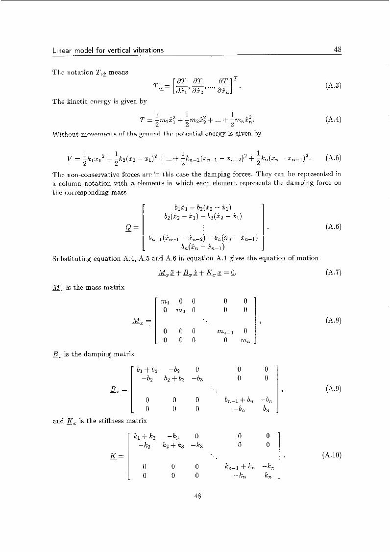
Linear model for vertical vibrations 48
- - ml O O O O
O m2 O O O
o O 0 772,-1 0 o O 0 0 mn -
nir,=
The notation T, , means T
- OT Ó’T
The kinetic energy is given by
1
Withmt mnoements of the groimd the potential energy is given by
& =
The non-conservative forces are in this case the damping forces. They can be represented in a column notation with n elements in which each element represents the damping force on
- bi + b2 -b2 0 O O -b2 b2 +b3 -b3 O O
O O O bn-1 + bn -bn - O O O -bn bn
the corresponding mass
- & =
b1k1 - b2(k2 - 21)
bz(k2 - 21) - b3(k2 - 51) l . ( A 4
‘1 bn-l(kn-l - lL.,-2) - b,(lL., - kn- l ) bn(2n - kn- i )
Substituting equation A.4, A.5 and A.6 in equation A.l gives the equation of motion
- K =
-1 + - 2 4 2 0 O O --2 -a+-3 --3 O O
(A.lO)
48

49 Linear model for vertical vibrations
A.l Movement of the ground
When movements of the ground are included in the model the equation of motion of the first mass changes t o
mi21 + (b i + b2)gi + ( k i f k2)xi = b222 + k 2 ~ 2 + bilcg + k l ~ , . (A.ll)
Now the equations of motion can be written as
M.,. 2 + B, ii + & 2 = €&gli.g + Kxgxg. (A.12)
Where &, B, and & are given by A.8, A.9 and A.10 respectively and and cg by
O
O O
Suppose that all movements are harmonic,
(A.13)
(A.14) (A.15)
then for the complex transfer function follows
&,(u) = = X = ( -M -w2 + B,iw +&)-I * (B,,iw + Kxg). (A.16) x9
The complex transfer function is a column in which element i represents the complex response of mass i t o harmonic movements of the ground.
A.2 Approximations for high frequencies
The equation of motion in the frequency-domain can be written as
(-&w2 + B , i w + &)X = (B,,iw + G g ) X g . (A.17)
Or by n equations

Linear model for vertical vibrations 50
Abbreviating the coefficients yields
(A.19)
Solving these equations yields
(A.20)
For higher frequencies only the terms with the highest order of w remain in the numerator and denominator. So for higher frequencies follows
2 1 2 2 . . .zn- 12, A1A2 ... An-lAn - O ( W ~ , - ~ ) ’
5- - 21 2,. . .z,- 12, - -
X, A1A2 ... An-lA, - AlA2A3 ... An-2Z, - ...
- - - X, AiA2 ... A,-iA,.
For medium frequencies and with k; > b; a fairly good approximation is
and finally for high frequencies follows
(A.21)
(A.22)
(A.23)
A.3 Calculation of eigenfrequencies and eigenvectors
The eigenfrequencies and eigenvectors of the the system are determined by going t o a state space notation. The n second-order equations are written as 2n first order equations by making use of 2n states: the displacements and the velocities of the n masses. The space vector is given by - -
Now the equations of motion can be written as 2n first order equations
_ _ CIC* +Dg* = 0. Solutions of this equations are written as
* At - x*( t ) =go . e .
(A.24)
(A.25)
(A.26)
(A.27)
50

Linear model for vertical vibrations 51
Then the eigenvalue problem is represented by
[AC + Olio* = o. (A.28)
This problem can be solved by using standard numerical methods like EIG in MATLAB which gives the eigenvalues and eigenvectors as functions of c and 0.
A 4 Stiffness factors
Metal rods
The axial stiffness of a metal rod is calculated by
E A k = - . 1
(A.29)
With E the Young's modulus and 1 the rod length. The minimum cross section area A is determined by the load M g ) the yield strength amax and the safety factor a
Substituting A.30 in A.29 results in
(A.30)
(A.31)
Rubber disks
The axial stiffness of rubber disks is calculated in the same way as the stiffness of metal rods
(A.32)
With h the height of the rubber disk. The maximum stress in rubber disks (omax) depends on the stress concentration factor e,, which for a circular disk with radius d is defined as
d c c = 4h' (A.33)
A high stress concentration factor implies that the maximum stress in the disk can be higher than with a low concentration factor. This dependence is presented in material handbooks by diagrams.
Helium bellows
The stiffness of a helium bellow with loaded area A and height h can be calculated by
d F dP dh d h '
5 = -- = -A- (A.34)
The relation between pressure and volume is determined by the compressibility factor p, defined as
(A.35)
51

Linear model for vertical vibrations 52
With V the volume of the bellow : V = m 2 h = Ah. Where r is the radius of the bellow. Substituting this in A.35 gives
(A.36)
The minimum loaded bellow area is determined by the maximum pressure for helium before it solidifies
ML2 A = pmax,He
Substituting A.36 and A.37 in A.34 gives
(A.37)
(A.38)
In fact the helium bellows are metal bellows filled with liquid helium. The stiffness of the metal bellows (N 8.5 .lo5 N/mZ), however can be neglected with respect to the stiffness of the helium column (N 2.3 lo7 N/m2).
A.5 Damping factors
The damping in each element is given by the dimensionless damping factor [i. This factor represents the fraction of critical damping be;,
b; = Eb,; = 2 E G . (A.39)
The dimensionless damping factor depends on the type of connection element in the sus- pension. This fraction is for a metal rod lower than for a helium damper for example. The values for the dimensionless damping factors are estimated and should be adjusted when more information about the real system design is available.
A.6 Data standard configuration
The standard configuration consists of eight masses. The composition of the system is given in Table A.1. The dimensions and physical characteristics of the used materials are given below:
Number of masses n = 8 Safety factor o! = 3 Length rod stage 2: 2.5 m Length rods stage 4: 1.6 m (3 rods in parallel) Length rods stage 6: 1.6 m (3 rods in parallel) Length rod stage 8: 3.0 m Height helium dampers: 0.2 m
In the alternative configurations rubber and steel disks are added to the room temperature level of the suspension. The data for these disks are:
Mass steel disks: 500 kg
52

Linear model for vertical vibrations 53
Stage i 2
Height rubber disks: 0.20 m
Body ' Mass [kg] 1 Voanection ' R [m] I k [ . 108 N / ~ I ' '
Support (Concr.) 200.000 I 12 Air bellows 5.0 I 0.3 0.030 Interm. mass (Cu)
Table A.l: Standard configuration for vibration isolation system of GRAIL con- sisting of eight masses. R is the distance from the connection to the x-axis of the suspension.
Material omax [N/m2] Steel 2.4 a l O s
E [N/m2] G [N/m2] p [kg/m3] v 2.10 .lo1' 8.08 .lo1' 7.8 .lo3 0.3
5.000 I 1 Titanium rod I 0.0 I
Copper Titanium Neoprene
1.76
2.7 a l O s 1.23 .lol1 4.70 -lo1' 8.9 . lo3 0.33 7.6 -10' 1.05 .lol1 3.87 . lo8 4.5 . lo3 0.35 3.2 -lo6 3.00 - lo7 1.30 - lo6 1.3 .lo3
I 0.005 I
Table A.2: Physical characteristics of used materials.
53

Linear model for vertical vibrations 54
54

Appendix B
Linear model for torsional vibrations around the vertical axis
To examine the vibrations around the vertical axis of the detector a linear model with torsional springs and torsional dampers is used, see Figure B.1. The equation of motion are written as
Figure B.l: Linear model for torsional vibrations.
Where 9 is the column with rotations of the masses around the x-axis: - y = [vl, p2, p3, ..., 9,IT and yg?s the rotation of the ground around the x-axis.
55

Linear model for torsional vibrations around the vertical axis 56
M is the mass matrix -<p
Where Jz; is the mass moment of inertia around the x-axis, calculated by 1/2mr2 for a circular disk an by 2/5mr2 for a sphere. I?,, K,, and Kqg are similar t o respectively A.9, A.10 and A.13. Of course the values for b; and k; are different.
B. l Stiffness factors
Metal rods
The torsional stiffness parameter for the metal rods is a combination of torsion, bending and the gravitational effect, depending of the position of the rods in the structure, see Figure B.2. The gravitational effect takes place for rods which are placed out of the x-axis of the detector and implies that masses which hang on that rod are lifted a little bit in the gravitational field.
t
Torsion
1 t
Bending
t
Gravitation
Figure B.2: Three effects for torsional stiffness.
The torsion effect for one rod is represented by
Where G is the shear modulus and I the rod length. The polar moment of inertia IP is $7rr4, where r is the radius of the rod.
The bending stiffness for three equally distributed rods in parallel is
36EIR2 13
k b = 03-41
Where I is the moment of inertia of the rod cross section around the y-axis ( I = a7rr4) and R is the distance between the rod and the vertical axis of the detector.
The gravitational effect is caused by the fact that the potential energy increases by rotation of the lower mass for small angles with a factor
56

Linear model for torsional vibrations around the vertical axis 57
d~ = m t g l ( 1 - COS -). Rv I
With mt the total mass hanging on the parallel rods. The stiffness factor for the gravitational effect for small angles results in
mtgR2 kg = 7 Foï rods which are positioned abng the x-axis the total stiffness factor is given by k = kt.
For rods which are positioned at a distance R from the axis of the detector the total stiffness factor is given by k = 3kt + kb + ik,. Rubber disks
The rubber disks are placed on the x-axis of the detector so only the torsion effect participates in the torsion stiffness
(B.7) GIP kt = - h
Where G is the shear modulus of rubber and h is the disk height. The polar moment of inertia Ip is calculated by i7rr4, where r is the radius of the disk.
Bellows
For the helium and air-bellows the shear stiffness and torsional stiffness are taken into account. The torsional stiffness of bellows is calculated by
GIP kt = - I ’
where G is the shear modulus for the bellow material and I p is approximated by Ip N 271-Sr3 with r the radius and S the thickness of the bellows.
The shear stiffness for rotations is calculated by making use of the horizontal shear stiffness of the bellows. The total torsional stiffness coefficient is calculated by
Where k , is the horizontal shear stiffness factor of the bellow.
B.2 Damping factors
The damping in each element is given by the dimensionless damping factor t;. This factor represents the fraction of critical damping bei,
b; = [bc; = 2 t a . (B.lO)
The dimensionless damping factor depends on the type of connection element in the suspen- sion. The values for the dimensionless damping factors are estimated and should be adjusted when more information about the real system design is available.
57

Linear model for torsional vibrations around the vertical axis 58
58

Appendix C
Linear model for horizontal vibrations
To examine the horizontal vibrations of the suspension a linear model with springs and dampers is used (see Figure C.1). Due t o symmetry around the vertical axis, the model for vibrations along the y-axis is the same as for vibrations along the z-axis. The equations
e
Figure C.l: Linear model for horizontal vibrations.
of motion read
My y + By y + i c y y = B y g i g + KygYg.
Where y is the coli mn with horizontal translations of the masses: yo is t h e horizontal translation of the ground.
!= lY1,
The mass matrix My, damping matrix By, stiffness matrix Ky and the matrices and
59

Linear model for horizontal vibrations 60
-YQ K the same. The values for b; and k; are different.
are similar t o respectively A.8, A.9, A.10 and A.13. The values for the masses m; are
c.1 Stiffness factsrs
For horizontal vibrations in the suspension three effects are taken into account. The lateral stiffness is calculated for helium bellows, air bellows and rubber disks. For metal rods the bending siiEness and gravitational e-f-fect are taker, i ~ t o acceunt.
Metal rods
The horizontal stiffness parameter for the metal rods is determined by the bending effect and the gravitational effect. The bending stiffness for one rod is calculated with
and for three rods in parallel with
36EI kb = -
13 . Where E is the Young’s modulus and 1 the rod length. The moment of inertia of the rod cross section around the y-axis I is calculated by + 7 r i 4 , where T is the radius of the rod.
For deriving a stiffness factor representing the gravitational effect a so called double pen- dulum is analysed which is shown in Figure C.2. The kinetic energy of this system is given
Figure C.2: Double pendulum.
The potential energy is given by
v = -mig11 cosy1 - m z g ( l 1 cosy1 + 12 cosya).
60
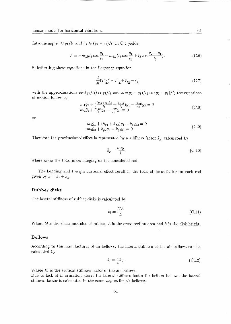
Linear model for horizontal vibrations 61
Introducing y1 N y1/21 and 7 2 N (y2 - yl)/l1 in C.5 yields
1. Y2 - Y1 v = -mlgZl cos - Y1 - mZg(Z1 cos - Y1 + Zz COS ~
I1 I1 z2
Substituting these equations in the Lagrange equation
(C.7)
m1$1+ (kgl + kg2)Yl - kg2Y2 = 0 mziz + kgzY2 - kg2Y1 = o.
Therefore the gïavitatiûna! effect is ïepresefited by a stiffness fxt,or kg, ca!r,u!ated by
mt g kg = 7,
where mt is the total mass hanging on the considered rod.
(C.10)
The bending and the gravitational effect result in the total stiffness factor for each rod given by 5 = kb f kg.
Rubber disks
The lateral stiffness of rubber disks is calculated by
GA h
= - (C.11)
Where G is the shear modulus of rubber, A is the cross section area and h is the disk height.
Bellows
According t o the manufacturer of air-bellows, the lateral stiffness of the air-bellows can be calculated by
(C.12) 1 4
kl = -IC,.
Where k , is the vertical stiffness factor of the air-bellows. Due to lack of information about the lateral stiffness factor for helium bellows the lateral stiffness factor is calculated in the same way as for air-bellows.
61
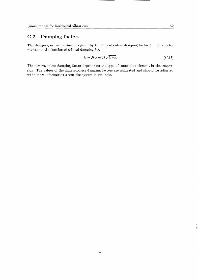
Linear model for horizontal vibrations 62
C.2 Damping factors
The damping in each element is given by the dimensionless damping factor e;. This factor represents the fraction of critical damping b,;,
(C.13)
The dimensionless damping factor depends on the type of connection element in the suspen- sion. The values of the dimensiímless d a m p i ~ g fzctors are estimated and shoiild be adjilsted when more information about the system is available.
62
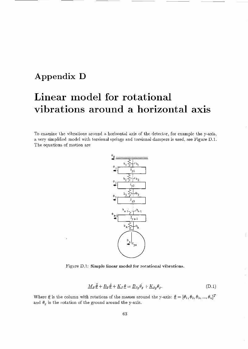
Appendix D
Linear model for rotational vibrations around a horizontal axis
To examine the vibrations around a horizontal axis of the detector, for example the y-axis, a very simplified model with torsional springs and torsional dampers is used, see Figure D.l. The equations of motion are
Figure D.l: Simple linear model for rotational vibrations.
Where @ is the column with rotations of the masses around the y-axis: and û, is the rotation of the ground around the y-axis.
= [81, &,83, ..., 8,IT
63
Linear model for rotational vibrations around a horizontal axis 64
- - Jyi 0 0 O O
0 Jy2 0 O O
o O 0 Jyn-1 0 o O 0 0 Jyn -
& =
~
Ado is the mass matrix
‘ahere ~~i is the mass moment cf inertiz. aroiind the x-axis caiciiiated by ~ j d r n r ~ tor a circular disk and by 2/5mr2 for a sphere. Bg, I&, l3,, and Keg are similar t o respectively A.9, A.10 and A.13. The values for b; and ki are different.
D. I Stiffness factors
The stiffness factors for all connections are calculated with the assumption tha t the masses rotate around their centres of mass. This is a very simplified assumption and implies that no masses are tilted in the gravity field. Therefore no stiffness factors due t o gravitational effects are included.
Metal rods
The stiffness parameter for the metal rods are calculated by:
kt = R2k,. (D-3) Where R is the distance between the rod and the vertical axis and kv is the vertical stiffness of that rod. For metal rods which are placed on the x-axis of the detector an arbitrary (low) stiffness coefficient is chosen. These coefficients are arbitrary chosen because a stiffness coefficient equal to zero results in a singular stiffness matrix.
Rubber disks
The rubber disks are placed on the x-axis of the detector so equation D.3 cannot be used. For these disks also an arbitrary (low) stiffness coefficient is chosen.
Bellows
The helium and air-bellows are placed out of the x-axis of the detector so the stiffness factors are calculated by
Where k, is the vertical stiffness factor of the bellow and R the distance between the bellows and the x-axis.
kt = R’k,. P . 4 )
D.2 Damping factors
The damping in each element is represents the fraction of critical
given by the dimensionless damping factor <i. This factor damping bc;,

Linear model for rotational vibrations around a horizontal axis 65
The dimensionless damping factor depends on the type of connection element in the suspen- sion. The values for the dimensionless damping factors is estimated and should be adjusted when more information about the system is available.
65

Linear model for rotational vibrations around a horizontal axis 66
66

Appendix E
Active control
In this appendix a feedback system for the reduction of transmitted vibrations from an un- predictable source is examined. First a system with only one degree of freedom which uses the PD control strategy is examined. Secondly this strategy is used for a multiple degree of freedom system.
In Figure E.l a mass is suspended by a spring and a damper. The controller R determines
Figure E.l: One degree of freedom control system consisting of a mass suspended by a spring and damper and an additional active element.
a control force F which should be applied t o the mass as a result of the displacement and velocity characteristics of the mass. This force is calculated using the relation
The purpose of attaching the active element t o the system is to fix the mass in a certain position. This means that
zdl( t ) = 0 ; k d l ( t ) o. Introducing condition (E.2) in equation (E.l) yields
67

Active control 68
Now the equation of motion of the mass can be written as
mx + bk+ kx = bkg + kxg + F j mx + (b + Krd)k + ( k + K)x = bkg + kxg . 03-41
For the frequency domain the following equation is obtained
- = (--Si,W2 + ( b + KTd)iLJ + (ik + K>>-' . (&U + k ) . Xg (E.5) X
In Figures E.2 and E.3 the response function (E.5) is given for various values for respectively K and r d . In both cases also the response function for the system without active control is given. The values for m, k and b are: m = 10 kg, k = 1.0. lo5 N/m and b = 100 N/ms. In Figure E.2 Td = 0.005 s. In Figure E.3 I< = 5.0 - IO4 N/m. The amplification constant K has a major influence in the low frequency region. Where the transfer function for the uncontrolled system converges t o 1, the controlled system has a transfer function which is lower than 1. In this region the transfer is determined by K . For high frequencies the transfer function for the controlled system equals the transfer function for the uncontrolled system. The time constant r d only has influence in the neighbourhood of the resonance frequency. It determines mainly the peak height.
68

Active control 69
Figure
Figure E.3:
= 0.005 S.
Frequency [Hz]
Transfer functions with various values for Td and I< = 5 .O . l o4 N/m.
69

Active control 70
In order t o analyse the behaviour of the control system often a block diagram is drawn. This is represented in Figure E.4 for the control system with one degree of freedom.
x,(t> . Hg(4
hi,
Figure E.4: Block diagram of the control system
A block H ( s ) gives the Laplace function of the transformation of the input signal ( s = iw). The first block Hr(s ) represents the PD-controller with transfer function
H r ( S ) = 11'(1 + Tdds). (E4 The input signal e ( t ) is the error signal, representing the difference between the desired
position of the mass and the real position: e ( t ) = zd(t) - z ( t ) . The disturbing signal n(t) which comes from the moving ground is given by n(t) = bk, + k z , . Therefore the transfer function becomes
H,(s) = bs + k . 03.7) The force signal F ( t ) which is the output of the controller together with the disturbing signal n(t) yields the input signal for the process block H,(s). For this block the following transfer function is valid
Now the output signal results in
H p N . 1 + HrHp
X ( s ) = H r H p xd+ 1 + HrHp
According t o Equation E.2 follows X ~ ( S ) = O , so for the output signal results
bs+k X ( s ) = H p H g X , = K(1+ T ~ S ) + ms2 + bs + 5 x, 1 + HrHp
(E.lO)
Note that with s = iw the same transfer function is obtained as given in Equation (E.5).
For the multiple degree of freedom system with n masses the same control strategy as used for the system with one degree of freedom is applied (see Figure E.5).
Comparing the controlled multiple degree of freedom system with the uncontrolled system (see Appendix A), only the equation of motion of the first mass differs. The equation of this mass becomes
70
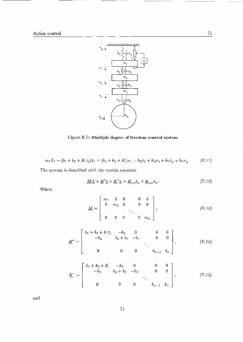
Active control 71
Figure E.5: Multiple degree of freedom control system
The system is described with the matrix equation
_- M 2 + + -*i = &,ag + &,xg. Where
ml O O O 0 O m2 O O 0
- M = I o o o * . * o
(E.12)
(E.13)
and
71

Active control 72
&g =
b l O
O
Then for the transfer function If: follows
O
O
X H* = = = (-Mu2 + B*iu +-*)-I . (B,,w + i,,). xL7
(E.16)
(E.17)
72
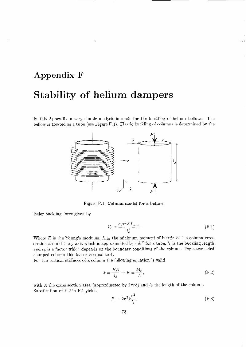
Appendix F
Stability of helium dampers
In this Appendix a very simple analysis is made for the buckling of helium bellows. The bellow is treated as a tube (see Figure F.l). Elastic buckling of columns is determined by the
....
....
Figure F.l: Column model for a bellow.
Euler buckling force given by
Where E is the Young’s modulus, Imin the minimum moment of inertia of the column cross section around the y-axis which is approximated by rSr3 for a tube, 11, is the buckling length and Cb is a factor which depends on the boundary conditions of the column. For a two sided clamped column this factor is equal to 4. For the vertical stiffness of a column the following equation is valid
with A the cross section area (approximated by 2 n d ) and Ik the length of the column. Substitution of F.2 in F.l yields
r2 Ik
F, = 2n2k-.
73

Stability of helium dampers 74
The stiffness factor k for the helium bellows cannot be calculated by Equation F.2 but is determined experimentally and given in handbooks by the manufacturer. For an iron bellow a stiffness factor of 8.5 . l o5 N/m is given. With a radius of 0.2 m and height of 0.22 m the buckling force is 3.05 lo6 N. So each bellow can resist for about 300.000 kg before i t buckles. This load is much higher than the maximum force when the helium solidifies so the solidification criterion gives the critical load. I t can be concluded here that the helium bellows won’t buckle if properly designed. For a more detailed analysis in which the diEcu!t grxxetry ~f the bellow is taken into account a special method has to be used [17].
74

Appendix G
Vibrations of a continuous rod
In this appendix longitudinal and transverse vibrations of a continuous rod loaded with an end mass is examined.
G . l Longitudinal vibrations r
in Figure G.1 a one sided clamped rod is given with a mass attached at the other end.
Figure G.l: Continuous rod with a mass attached at the end.
For free longitudinal vibrations in a continuous rod the following differential equation is valid
Where c is the wave constant ( e = m), E the Young's modulus and p the material density. The solution of this equation can be expressed as
wx u(x , t ) = ( A ~ cos(=) c + A~ sin(-)) c ( B ~ cos(wt) + B~ sin(wt>>. (G.4
Where the values for A l , A2, B1 and B2 follow from the boundary conditions. The boundary conditions in this case are
75

Vibrations of a continuous rod 76
u = U,sinwt for x = O
m- = -EA- f o r z = l . d 2 U au d t 2 dx
With B2 = 1 then follows
Al = U, mw2U, cos % + EAU,: sin $
EA; cos + - mw2 sin $ A2 =
BI = o. Now for longitudinal vibrations of the rod the following equation is obtained
4 t) - E A u(0, t ) EA cos - mcw sin $.
-
The resonance frequencies w, can be calculated from
wnl wnl EA cos - - mew, sin - = O c c
or a t a n a = p.
(G.lO)
(G.11)
With (I! = w,l/c and ,8 = AEl/mc2 = m,/m where rn, is the mass of the rod. These resonance frequencies must be calculated with a numerical method by lack of an analytical solution. The mass-spring model for this rod is given in Figure G.2. The equation of motion is expressed
1 x,u
EA k - t 1
Figure G.2: Mass-spring model for a rod.
76

Vibrations of a continuous rod 77
as
SO the transfer function becomes
(G.12)
((3.13)
Note that if c >> wl Equation G.9 equals the transfer hnction for the mass-spring model. The rod cross section area A is calculated from
(G.14) A = - . amg omax
Where o,,,, is the yield strength and Q is the safety factor.
G.2 Transverse vibrations
For free transverse vibrations in a slender rod the differential equation originally derived for a string can be used
,d2v d2v e - = - ax2 at2.
(G.15)
Where c i s the wave constant ( e = Jp/p*), P the tension ( P = mg) and p* the linear mass density (mass per unit length). The solution of this equation is the same as given in Equation G.2. The boundary conditions in this case are
v ( x , t ) = V,sinwt for IC = 0 m- a 2 V = -P- d V f o r x = l .
a t 2 dX Now for transverse vibrations of the rod follows
For x = 1 this is reduced to
V ( l > t ) - 1 -
~ ( 0 , t ) cos + - s s i n $ ' 9
Now the resonance frequencies wn can be calculated from
wnl wnc . wnl cos---sin-=O.
(G.16)
(G.17)
(G.18)
(G.19)
(G.20) c 9 c
The lowest resonance mode (n=O) represents the pendulum mode (oo N wp = m). Higher resonance modes are so called violin modes. The resonance frequencies can be approximated bv
w, N n r w p F n = 1,2 , ... mr
(G.21)
77

Vibrations of a continuous rod 78
Where m, is the mass of the rod. The same results are found by Mio [13] Transfer functions for transverse vibrations for a system with more masses like the me-
chanical suspension of GRAIL can be calculated in the same way as for one mass. However, these calculations are beyond the scope of this thesis.
78

Appendix H
Random vibrations
In this appendix some definitions and formulas are given for signal characterization in the frequency domain [ia].
The Fourier transform of a random signal z ( t ) observed during a period T is given by
The autopowerspectrum or power spectral density is defined by
S,,(f) = E [ lim X ( T , f)X(T, !)l. T+W
The autocorrelation function is given by
B,,(T) = lim /T '2 z ( t ) z ( t + 7)dt. T+m -Ti2
The autopowerspectrum and the autocorrelation are each others Fourier transforms:
00
S,,(f) = 1 RZ,(T)eëaTirjfTdT,
R&) = lcc S,, (r)e2"jfTdf.
7=-00
f=-cc
The transfer function of two signals z ( t ) and y ( t ) is given by
Y ( f ) = H ( f ) X ( f ) (H.6) Theoretically it is possible to determine the transfer function of two measured time signals during a period T by H ( f ) = Y ( T , f ) / X ( T , f ) . In practice this equation is not used due to difficulties caused by the phase information of the Fourier transforms. In practice it is usually calculated by
with S,,(f) the cross-power spectrum, defined by
79