gravitational lensing, rational functions, and rubber bands

Gravitational Lensing Thurston Maps Rubber Bands and Elastic Graphs An Example

Gravitational Lensing, Rational Functions, andRubber Bands

Lukas Geyer

Montana State University

SIAM Northern States Meeting, Laramie, WY

September 27–29, 2019

Interactions among Analysis,

Optimization, and Network Science


Outline

1 Gravitational Lensing

2 Thurston Maps

3 Rubber Bands and Elastic Graphs

4 An Example


Gravitational Lensing I

Gravitational lenses observed by the Hubble space telescope


Gravitational Lensing II


The Lens Equation

The Lens Equation

z =

∫C

dµ(ζ)

z − ζ+ w

where

w : Actual position of light source

z : Apparent position of light source

µ: Mass distribution of lens (up to physical constants)

Everything projected to the lens plane P which is identified with C.

Remark

This equation might have many (even infinitely many) solutions zfor given w .


The Lens Equation for Point Masses

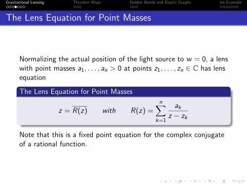
Normalizing the actual position of the light source to w = 0, a lenswith point masses a1, . . . , an > 0 at points z1, . . . , zn ∈ C has lensequation

The Lens Equation for Point Masses

z = R(z) with R(z) =n∑

k=1

akz − zk

Note that this is a fixed point equation for the complex conjugateof a rational function.


Number of Lensed Images

Question

How many apparent images of a single light source can a lens withn point masses generate?

For n = 1 calculation is elementary:

If z1 = 0 (light source and lens object aligned), the image is acircle (Einstein ring)If z1 6= 0, the answer is always 2. (One of the lensed imageswill be too close to the lens itself to be visible.)

For n ≥ 2 the number of images Ln always satisfies

n + 1 ≤ Ln ≤ 5n − 5

and the bounds are sharp.(Sharp lower bound: Petters 1991; Upper bound: Khavinson, Neumann 2006; Sharpness: Rhie 2003)


Counting Solutions

Generically, all fixed points z = R(z) are either

attracting, i.e., |R ′(z)| < 1, or

repelling, i.e., |R ′(z)| > 1,

in which case we get

Lefschetz Identity (or Harmonic Argument Principle)

L− − L+ = n − 1 and L = 2L+ + n − 1

where

L+: Number of attracting fixed points

L−: Number of repelling fixed points

L = L+ + L−: Total number of fixed points


Extremal Lensing Configurations

Definition

A lens configuration of n ≥ 2 points is extremal if it generates themaximum number 5n − 5 of lensed images. The correspondingrational map R is an extremal rational map.

From the definition of R and the Lefschetz Identity we get

Definition

A rational map R of degree n ≥ 2 is extremal iff

R(∞) = 0,

R has only simple poles with positive real residues, and

z 7→ R(z) has 2n − 2 attracting fixed points.


Extremal Polynomials

Motivated by a conjecture of Wilmshurst on the number of zerosof complex harmonic polynomials, the following is known on thepolynomial analog of the lens equation:

Theorem (Khavinson, Swiatek 2003)

Let P be a polynomial of degree n ≥ 2. Then the number ofsolutions of z = P(z) is at most 3n − 2.

Theorem (G. 2008)

For every n ≥ 2 there exists a polynomial P of degree n such thatthe number of solutions of z = P(z) is equal to 3n − 2.


Counting Extremal Polynomials

The second theorem follows from:

Theorem (G. 2008)

For every n ≥ 2 there exists a real polynomial P of degree n withdistinct critical points c1, . . . , cn−1 such that ck = P(ck) fork = 1, . . . , n − 1. Furthermore, the number of equivalence classesof such polynomials is given by

En = Cb(n−1)/2c where Cm =1

m + 1

(2m

m

).

Extremal polynomials are represented by Hubbard trees.

(Cm) are the Catalan numbers, which count finite rootedsubtrees of an infinite rooted binary tree.


Extremal Rational Functions

Question

Is there a family of combinatorial objects representing extremalrational functions?

Hubbard trees encode the topological dynamics ofpost-critically finite polynomials.

Properties of Hubbard trees guarantee that this topologicalmodel can actually be realized by a polynomial.

Post-critically finite topological rational functions can berealized iff they do not have a Thurston obstruction.

Obstructions for rational functions are more complicated thanfor polynomials.


Rubber Bands and Elastic Graphs

Dylan Thurston (partially with Jeremy Kahn and Kevin Pilgrim)has recently given a new criterion for topological equivalence ofThurston maps to rational maps, using rubber bands aka elasticgraphs.

Example

An extremal lensing map for n = 3 is given by

R(z) =az2

z3 + 1with a =

3

21/3

Critical points are z0 = 0 and zk = 21/3e2πik/3 for k = 1, 2, 3,satisfying zk = R(zk).


Constructing an Elastic Graph for R

We need a spine Γ of C \ {z1, . . . , z4} for the map R, and itspreimage Γ = R−1(Γ).

Definition

An elastic structure on Γ is a metric α on Γ, Lipschitz equivalentto (spherical) length.

Definition

For a Lipschitz map φ : Γ→ Γ, the embedding energy is

Emb(φ) = supy∈Γ

∑x∈φ−1(y)

|φ′(x)|,

where |φ′(x)| is taken with respect to α and R∗α.


Equivalence to Rational Maps

Theorem (D. Thurston 2016)

Let R be a Thurston map with post-critical set P and assume thatthere is a branch point in each cycle in P. Then R is equivalent toa rational map iff there is an elastic graph spine (Γ, α) for C \ Pand a map ψ ∈ [φn] with Emb(ψ) < 1.

Here [ψn] is the homotopy class of the “projection” R−n(Γ)→ Γ inC \ P. In “nice” cases one can take n = 1.


Constructing an Elastic Graph I


Constructing an Elastic Graph II


Collapsing an Elastic Graph I


Collapsing an Elastic Graph II


Collapsing an Elastic Graph III


Future Work

Next steps:

Construct elastic graphs for the known extremal lensing mapsfor n ≥ 3, given by

R(z) =azn−1

zn + 1+

b

z

with suitably chosen a > b > 0.

Characterize spine pairs (Γ,R−1(Γ)) corresponding toextremal lensing maps combinatorially/topologically.

Construct other extremal lensing maps, or show that these donot exist.


Thank You!

gravitational lensing, rational functions, and rubber bands

Documents