grassland modeling and monitoring with spot-4 ......agricultural and forest meteorology 105 (2000)...

Agricultural and Forest Meteorology 105 (2000) 91–115

Grassland modeling and monitoring with SPOT-4 VEGETATIONinstrument during the 1997–1999 SALSA experiment

P. Cayrola,∗, A. Chehbounib, L. Kergoatc, G. Dedieua, P. Mordeleta, Y. Nouvellond

a CESBIO (CNRS/CNES/UPS), 18 av. E. Belin, bpi 2801, 31401 Toulouse Cedex 4, Franceb IRD/IMADES, Col. San Benito, 83190 Hermosillo, Sonora, Mexico

c LET (CNRS/UPS), 13 av. col. Roche, BP 4403, 31405 Toulouse Cedex, Franced USDA-ARS, 2000 E. Allen Road, Tucson, AZ 85719, USA

Abstract

A coupled vegetation growth and soil–vegetation–atmosphere transfer (SVAT) model is used in conjunction with datacollected in the course of the SALSA program during the 1997–1999 growing seasons in Mexico. The objective is to provideinsights on the interactions between grassland dynamics and water and energy budgets. These three years exhibit drasticallydifferent precipitation regimes and thus different vegetation growth.

The result of the coupled model showed that for the 3 years, the observed seasonal variation of plant biomass, leaf areaindex (LAI) are well reproduced by the model. It is also shown that the model simulations of soil moisture, radiative surfacetemperature and surface fluxes compared fairly well with the observations.

Reflectance data in the red, near infrared, and short wave infrared (SWIR, 1600 nm) bands measured by the VEGETATIONsensor onboard SPOT-4 were corrected from atmospheric and directional effects and compared to the observed biomass andLAI during the 1998–1999 seasons. The results of this ‘ground to satellite’ approach established that the biomass and LAIare linearly related to the satellite reflectances (RED and SWIR), and to vegetation indices (NDVI and SWVI, which is aSWIR-based NDVI). The SWIR and SWVI sensitivity to the amount of plant tissues were similar to the classical RED andNDVI sensitivity, for LAI ranging from 0 and 0.8 m2 m−2 and biomass ranging from 0 to 120 g DM m−2.

Finally, LAI values simulated by the vegetation model were fed into a canopy radiative transfer scheme (a ‘model to satellite’approach). Using two leaf optical properties datasets, the computed RED, NIR and SWIR reflectances and vegetation indices(NDVI and SWVI) compared reasonably well with the VEGETATION observations in 1998 and 1999, except for the NIRband and during the senescence period, when the leaf optical properties present a larger uncertainty. We conclude that aphysically-sound linkage between the vegetation model and the satellite can be used for red to short wave infrared domainover these grasslands. These different results represent an important step toward using new generation satellite data to controland validate model’s simulations at regional scale. © 2000 Published by Elsevier Science B.V.

Keywords:SVAT; Grassland; Semi-arid; VEGETATION; SWIR; SALSA

1. Introduction

Both natural (floods, fires, droughts, volcanoes, etc.)and human (deforestation, overgrazing, urbanization

∗ Corresponding author. Tel.:+33-5-61-55-85-24;fax: +33-5-61-55-85-00.E-mail address:[email protected] (P. Cayrol).

and pollution) influences are known to cause massivechanges in vegetation cover and dynamics. Drasticchanges in land surface properties, such as those oc-curring because of deforestation or the desertificationprocesses are likely to have climatic consequences.There is increasing evidence pointing towards the im-portant role played by land-atmosphere interactions

0168-1923/00/$ – see front matter © 2000 Published by Elsevier Science B.V.PII: S0168-1923(00)00191-X

92 P. Cayrol et al. / Agricultural and Forest Meteorology 105 (2000) 91–115

in controlling regional, continental and global cli-mate. The fluxes of energy, mass and momentumfrom the land-surface adjust to and alter the state ofthe atmosphere in contact with land, allowing the po-tential for feedback at several time and spatial scales.A better understanding of land atmosphere feedbackcould thus provide answers to questions regardingthe climatic implications of land use/cover change,land surface heterogeneity, and of atmospheric com-position. Model simulations (Bonan et al. (1992), andNobre et al. (1991) among others) have shown thatdrastic changes in vegetation type and cover causesignificant impacts on simulated continental-scale cli-mate. Avissar (1995) reviews examples of model andobservational evidence showing that regional-scaleprecipitation patterns are affected by land surfacefeatures such as discontinuities in vegetation type. Inaddition, fluxes of CO2 and other greenhouse gasesalso depend on the biophysical properties of the landsurface. Changes in land cover, land use and climatemodify the uptake and release of these gases, lead-ing to changes in their atmospheric concentrationswhich in turn may influence the global atmosphericcirculation.

Plant canopy regulates the exchanges of mass, en-ergy and momentum in the biosphere–atmosphereinterface. It dominates the functioning of hydrolog-ical processes through modification of interception,infiltration, surface runoff, and its effects on surfacealbedo, roughness, evapotranspiration, and root sys-tem affect soil properties. The amount of vegetationcontrols the partitioning of incoming solar energyinto sensible and latent heat fluxes, and consequentlychanges in vegetation levels will result in long-termchanges in both local and global climates and inturn will affect the vegetation growth as a feedback.In marginal ecosystems, such as arid and semi-aridareas, this may result in persistent drought and de-sertification, with substantial impacts on the humanpopulations of these regions through reduction in agri-cultural productivity, reduction in quantity and qualityof water supply, and removal of land from humanhabitability. It is, therefore, scientifically and sociallyimportant to study arid ecosystems so that the impactof management practices on the scarce resources canbe understood. In this regard, a better understandingof soil–vegetation–atmosphere exchange processes atdifferent time–space scale must be achieved in order

to document the complex interactions between theatmosphere and the biosphere.

During the last decades, vegetation models havebeen designed to simulate the seasonal and inter-annual variability in plant structure and function. Toprovide insights on the interaction between terrestrialecosystems and the atmosphere, some of these vegeta-tion models are now being coupled to soil–vegetation–atmosphere transfer-scheme (SVATs) (e.g. Lo Seenet al., 1997; Calvet et al., 1998a) and even interactwith atmospheric models (e.g. to meso-scale model,Pielke et al., 1997; or to GCM, Dickinson et al.,1998). However, the development of process-basedmodels is accompanied by increasing difficulties inobtaining values for the numerous parameters requi-red by the models. This has been pointed out by Guptaet al. (1998) in the case of hydrological models. Thevegetation models are also confronted by this calibra-tion problem (e.g. Calvet et al., 1998b). The calibra-tion of these models proves especially difficult andtime-consuming when regional and long-term simu-lations are to be carried out.

In this study, a coupled vegetation growth and SVATmodel (V–S model) developed and validated usingHapex–Sahel data (Cayrol et al., in press) has beenused to simulate surface radiation, turbulent heat andmass, liquid water and the control of water vapor andCO2 fluxes. Data collected during the semi-arid land–surface–atmosphere (SALSA) program (Goodrichet al., 2000) over grassland site in Mexico duringthree growing seasons (1997–1999) have been usedto assess the performance of the model.

The specific questions addressed in the paper are:1. Can this coupled model initially developed for the

Sahel environment be used in Mexico, and whatlevel of adaptation/calibration is required?

2. Can this model capture the consequences of the ob-served inter-annual variability of the precipitationin terms of surface fluxes and vegetation develop-ment?

3. Is it possible to monitor the surface biophysicalparameters using NDVI and/or SWVI as surrogatemeasures, the ‘ground-to-satellite’ approach?

4. Can the vegetation growth/SVAT model, whencoupled to a radiative transfer scheme, repro-duce the seasonal and the inter-annual surfacereflectance observed by the VEGETATION sensor,the ‘model-to-satellite’ approach?

P. Cayrol et al. / Agricultural and Forest Meteorology 105 (2000) 91–115 93

This paper is organized as follows. Section 2 describesboth the ground and satellite data sets collected during1997–1999 seasons. Section 3 presents a brief descrip-tion of the model and calibration procedure. Section4 presents an assessment of the performance and ro-bustness of the model. In Section 5, measurements ac-quired by the new VEGETATION sensor in 1998 and1999 are also related to biophysical parameters such asgreen biomass and leaf area index (LAI). Finally, wepresent a comparison between predicted and observedradiative variables (i.e. reflectances) using VEGETA-TION sensor. The V–S model was coupled with aradiative transfer model in order to assess its capabil-ity to simulate the seasonal variation of visible, nearinfrared and short wave infrared surface reflectances.

2. Site and data description

The study site is located in the upper San Pedrobasin (near Zapata village, 110◦09′ W; 31◦01′ N; el-evation 1460 m) and was the focus of the SALSAactivities in Mexico during the 1997–1999 field cam-paigns. The natural vegetation is composed mainlyof perennial grasses of which the dominant genus isBouteloua, and the soil is mainly sandy loam (67%of sand and 12% of clay).

2.1. Field data

A 7 m tower has been erected in the beginning of1997 season and equipped with instruments to measureconventional meteorological data (incoming radiationand net radiation at a height of 1.7 m with REBS Q6net radiometer). The soil heat flux was estimated us-ing six HFT3 plates from REBS Inc., WA, USA. Windspeed and direction, precipitation, air temperatureand humidity were also measured. Soil moisture wasmeasured using Time Domain Reflectometry (TDR)sensors (Campbell Scientific CS615 reflectometer)at two locations and four different depths (5, 10, 20and 30 cm) and a capacity probe (ThetaProbe) whichgives an integrated measurement of the water contentover the first 5 cm of the soil layer. Radiative surfacetemperature was measured using Everest Interscienceinfrared radiometers (IRT) with a 15◦ field of view attwo different viewing angles (0 and 45◦). The bandpass of these radiometers is nominally 8–14mm.

Sensible and latent heat fluxes were determinedusing from the Eddy covariance method. The systemis made up of a three-axis sonic anemometer manu-factured by Gill Instrument (Solent A1012R) and anIR gas analyzer (LI-COR 6262 model) which is usedin a close path mode. The system is controlled by aspecially written software, which calculates the sur-face fluxes of momentum, sensible and latent heat andcarbon dioxide. However, during a large part of the ex-periment, some problems with the LICOR instrumen-tation did not permit the derivation of latent heat andCO2 fluxes. Therefore, latent heat flux was derivedfrom measurements of sensible heat flux and avail-able energy at the surface as the residual term of thesurface energy budget. In 1998, an additional Bowenratio system has been installed in the same site for a 3weeks period. Note that the main source of uncertaintyconcerns the surface soil heat flux. Kustas et al. (1999)showed that uncertainty in soil heat flux is probablylarger that the 30% reported in Stannard et al. (1994).Braud et al. (1993) also pointed out the problem as-sociated with the estimation of latent heat flux as theresidual term of the energy balance equation giventhe uncertainty in available energy measurements.

The evolution of the biomass was monitored dur-ing the 1997–1999 growing seasons from day of year(DoY) 182–285. The adopted protocol was to cut10 samples of 1 m2 of biomass along a 100 m tran-sect. Then live phytomass and standing necromasswere separated and weighted and the samples wereweighted again after 48 h drying at 70◦C.

The LAI was determined from biomass and specificleaf area (SLA) measurements (Nouvellon, 1999). In1998, grass stomatal resistance was measured usingtwo automatic porometers (models MK3 and AP4,Delta T Devices, Ltd, Cambridge, UK).

2.2. Satellite data

Two satellite datasets were used to monitor vege-tation growth and decay. The first data set consists ofdaily NOAA/AVHRR images acquired by IMADES(Hermosillo, Mexico) during afternoon overpass fromJanuary 1997 to fall 1998. AVHRR red and nearinfrared top-of-the-atmosphere images were geomet-rically corrected, re-sampled to 1 km× 1 km reso-lution, calibrated by IMADES. We also processeddaily data acquired since April 1998 around 10:30


Table 1Listing of the variables, parameters and constants used in the vegetation-SVAT model

Symbol Definition Type

a, b Parameters for soil resistance parameterization (rss), a = 35118 andb = 10.517(Chanzy, 1991)

Parameter

as Coefficient for photosynthates allocation to the shoots compartments (0.53 atj1 and j2,after Nouvellon et al. (2000))

Parameter

cg Heat capacity of the soil (DeVries, 1963) VariableCa− Γ CO2 concentration gradient between leaf surface and chloroplast (Ca− Γ = 0.640 g CO2 m−3;

Williams and Markley, 1973)Parameter

Cp Specific heat at constant pressure (J kg−1 K−1) ConstantCq Exchange coefficient depends on atmospheric stability VariableC1, C2, C3 Soil transfer coefficients for moisture (Mahfouf and Noilhan, 1996) Variabled Zero plane displacement height for the canopy (m) Variabledn Rate of necromass decays (here,dn is set to 0.015; Le Roux, 1995) Parameterd1, d2 Depth of surface layer (10 cm), depth of the root zone (40 cm) Parameterea Vapor pressure at canopy reference height (mbar) Variableec, eg Canopy (0.98) and ground surface (0.96) emissivity (Lo Seen et al., 1997) Parameteresat(Ti ) Saturated vapor pressure at temperatureTi (mbar) Variablee0 Aerodynamic vapor pressure (mbar) at within-canopy source height VariableEg, Etr Soil evaporation, plant transpiration rates (kg m−2 s−1) Variablegr Growth respiration coefficient for roots (0.6 g CO2 g−1 DM; Amthor, 1989) Parametergs Growth respiration coefficient for shoots (0.49 g CO2 g−1 DM; Amthor, 1989;

Nouvellon, 1999) compartmentsParameter

G Ground heat flux (W m−2) Variableh, height Vegetation height (cm): 3.52+ 0.0073Ms (kg C ha−1) − 0.000024M2

s (kg C ha−1) VariableH, Hc, Hg Total, canopy, soil sensible heat flux (W m−2) VariableI Photosynthetically active radiation (W m−2) VariableIC Initial carbon storage (0.12 kg C m−2, modified from Le Roux (1995)) ParameterIr PAR level for whichrr equals 2rr min ParameterIs PAR level for stomata half-closure (25 W(PAR) m−2; Kergoat, 1998) ParameterI0 Incoming PAR at the top of the canopy (W m−2) Variablej1, j2 Phenological dates: maximum of vegetation, DoY 245 and end of the growing

season, DoY 250, respectively (observations in situ)Parameter

k Von Karman’s constant (∼0.4 unitless) Constantke Extinction coefficient for PAR radiation (0.5 unitless; Kergoat, 1998) ParameterLAI Leaf area index (m2 m−2) VariableLE, LEc, Leg Total, canopy, soil latent heat flux (W m−2) Variablems, mr Rate of maintenance respiration for shoots and roots Variablems0, mr0 Maintenance respiration rate for shoots (0.003 per day) and roots (0.0012 per day),

after Amthor (1989)Parameter

Ms, Mr , Mn Shoots biomass, roots biomass, standing necromass (kg C m−2) Variablen Attenuation coefficient of eddy diffusivity within the vegetation (2.5 unitless,

Shuttleworth and Gurney, 1990)Parameter

n′ Attenuation coefficient of wind speed within the vegetation (2.5 unitless, Shuttleworthand Gurney, 1990)

Parameter

P Precipitation reaching the surface (kg m2 s−1) VariablePc Hourly canopy photosynthesis (g C m−2) VariablePl Leaf photosynthesis rate (g C m−2 s−1) VariablePn Daily canopy photosynthesis (g Cm−2 s−1) VariableQ10 Factor for maintenance respiration (Q10 = 2) Parameterraa

a Aerodynamic resistance between within-canopy source height and above-canopyreference height (s m−1)

Variable

raca Bulk boundary layer resistance of the canopy (s m−1) Variable

rasa Aerodynamic resistance between ground surface (soil source) and within-canopy

source height (s m−1)Variable

rc Canopy resistance (s m−1) Variable


Table 1 (Continued)

Symbol Definition Type

rr Leaf level residual resistance (s m−1) to CO2 transfer Variablerr min Minimum residual resistance to CO2 transfer (137 s m−1, see Cayrol et al. (in press)) Parameterrs Leaf level stomatal resistance (s m−1) Variable

rCO2s Leaf stomatal resistance (s m−1) to CO2 transfer (rCO2

s = 1.6rs) Variablers min Minimum leaf stomatal resistance (100 s m−1, measured in situ) Parameterrss

a Soil surface resistance (s m−1) VariableRA, RAc, RAg Incoming long-wave radiation, long-wave radiation for the canopy and bare soil,

respectively (W m−2)Variable

Rn, Rnc, Rng Total, canopy and soil net radiation (W m−2) Variabless, sr Rate of senescence for the shoots and roots compartments Variabless0, sr0 Mortality coefficient for shoots (0.01 per day atj1, 0.025 per day atj2, linear interpolated

betweenj1 and j2) and roots (0.01 per day atj1 and j2), best guess modified fromLe Roux (1995)

Parameter

SLAo Specific leaf area atMs = 0 (30 m2 kg C−1, in situ measurements) ParameterT Daily average air temperature (K) VariableTa Air temperature at reference height (K) VariableTc Temperature at canopy surface level (K) VariableTg Ground surface temperature (K) VariableTmin, Tmax Minimum, maximum temperature for photosynthesis (283 and 333 K; Kergoat, 1998) ParameterTr Radiative temperature (K) VariableTrans Translocation of carbohydrates (0.0004 kg C m−2 per day, best guess) ParameterT0 Aerodynamic temperature (K) at within-canopy source height VariableT2 Deep soil temperature (K) Variableua Wind speed at reference levelzref (m s−1) Variableua Friction velocity (m s−1) Variableuh Wind speed at the top of the canopy (m s−1) Variablevpd Vapor pressure deficit (Pa) Variableweq Surface soil moisture when gravity balances capillarity forces (m3 m−3) Variablewfc Volumetric soil moisture at field capacity (0.16 m3 m−3, see text) Parameterwg Volumetric soil moisture of the surface layer (m3 m−3) Variablewsat Soil moisture at saturation (0.42 m3 m−3, estimated from soil texture

(clay = 12% and sand= 67%); Cosby et al., 1984)Parameter

wwp Volumetric soil moisture at wilting point (0.068 m3 m−3, see text) Parameterw1 Characteristic leaf width (0.005 m; Choudhury and Monteith, 1988) Parameterw2 Volumetric soil moisture of the root zone (m3 m−3) Variablezref Reference height above the canopy where meteorological measurements

are available (2 m)Variable

z0 Roughness length of the canopy (m) Variablez′

0 Roughness length of the substrate (m) Variableγ Psychrometric constant (mbar K−1) Constantλg, λ2 Ground and deep soil thermal conductivity (W m−1 K−1) Variableρ Density of air (kg m−3) Constantρw Density of liquid water (kg m−3) Constantσ Stephan–Bolztmann constant (5.67×10−8 W m−2 K−4) Constantσ f Screen factor (unitless),σf = 1 − exp(−0.8 LAI ) Variableτ Time constant of one day (s) Constantτp SVAT time step (s) Constant

a Resistances formulations can be found in Table 2.

LST by the VEGETATION instrument onboard SPOT-4 (http://sirius-ci.cst.cnes.fr:8080/). VEGETATION isa large field-of-view instrument providing measure-ments in four spectral bands, namely: blue (0.43–0.47

mm), red (RED, 0.61–0.68mm), near infrared (NIR,0.78–0.89mm) and short wave infrared (SWIR,1.58–1.75mm). The resolution is 1 km×1 km at nadirand is still better than 1.5 km at 50◦ viewing angle.


We used VEGETATION P-products, which consistof top of the atmosphere reflectance, geometricallycorrected and remapped with a multi-temporal andabsolute accuracy better than 1 km. A VEGETATIONdedicated version of SMAC (Berthelot and Dedieu,unpublished) was used for atmospheric corrections.Water vapor fields at 1× 1◦ resolution were derivedfrom atmospheric analyses of the French weatherforecast operational model available every 6 h. Thisprocedure for atmospheric correction is now used forthe operational processing of VEGETATION data.

VEGETATION and AVHRR sensors have a largefield of view, which implies large view zenith anglevariations from roughly 0 to±65◦. The reflectancescan vary by factors of two or three, depending on thesun-sensor geometry. This implies that these direc-tional effects have to be corrected. One of the optionsto minimize these effects is through the use of theso-called vegetation indices. Two vegetation indiceswere calculated: NDVI= (NIR−RED/(NIR+RED)

and SWVI= (NIR−SWIR)/(NIR+SWIR). Normal-ized reflectance were also computed to remove the ef-fect of surface anisotropy on the VEGETATION data,as described in Appendix A.

3. Model description and calibration procedure

3.1. Model description

An extensive description of the Vegetation-SVATmodel (V–S model) which is used in this study can befound in Cayrol et al. (in press). The mains equationssolved by the model are summarized in the AppendixB. Schematically, the vegetation growth model pro-vides the LAI, which is then used by the SVAT in the

Table 2SVAT resistances formulations

Formulationa Reference

raa (Cqua)−1 Mahrt and Ek (1984)

rac100

2n′LAI

√w1

uh

1

1 − exp(−n′/2)Choudhury and Monteith (1988)

rash exp(n)

n Kh

[exp

(−nz′0h

)− exp

(−n(z0 + d)

h

)]with Kh = ku∗(h − d) and u∗ = kua

ln((zref − d)/z0)Shuttleworth and Gurney (1990)

rss a exp(−bwg/wsat) Passerat de Silans (1986)

a All the symbols are defined in Table 1.

Fig. 1. Observed (5, s ande) and simulated (–, – – and –·) sea-sonal evolution of the aboveground biomass for years 1997–1999,respectively. Error bars indicate the standard deviation.

computation of the energy partitioning between soiland the vegetation as well as in the parameterizationof turbulent transport and evapotranspiration. This up-dates the soil water content in the root zone (w2), andthus tissue mortality rate. The stomatal conductanceis shared by both sub-models to compute transpirationand photosynthesis.

The surface scheme follows Shuttleworth andWallace (1985) approach. It considers soil and vegeta-tion as two different sources of latent and sensible heat


fluxes. The incoming energy is partitioned betweenbare soil and vegetation through a screen factor (σ f ).The dynamic of heat and water flux in the soil is de-scribed using the force-restore (Deardorff, 1978). Thecoefficients involved in the force-restore approach areparameterized as function of soil texture. The originalformulation of the force-restore coefficients was mod-ified in order to implicitly describe the vapor phasetransfers within the dry soil (i.e.wg < wwp) (Braud

Fig. 2. Precipitation (mm per 5 day) measured on the Zapata grassland site during (a) 1997, (b) 1998 and (c) 1999.

et al., 1993; Giordani et al., 1996), and to represent thegravitational drainage (Mahfouf and Noilhan, 1996).

The four prognostic equations for the SVAT modelare numerically solved for the following variables:surface temperatureTs, mean surface temperatureT2,surface soil volumetric moisturewg, total soil volu-metric moisturew2. The three prognostic equationsfor the vegetation growth model give the evolutionof the shoots biomassMs, the root biomassMr and


standing necromassMn. The V–S model is drivenby meteorological forcing variables, such as, air tem-perature, air humidity, wind speed, rainfall, and solarradiation. Additional surface characteristics, namely,soil parameters such as soil texture (% clay, % sand),soil thermal and hydraulic properties, root depth; andvegetation parameters such as SLA, maximum rate ofphotosynthesis are also prescribed (see Table 1).

3.2. Choice of the parameters, initialization andcalibration

As stated in the introduction, one of our objectivesin this study is to investigate the cost in terms of modelcalibration associated with the adaptation of a modeldeveloped and validated over a different site to a newsite. A distinction needs to be made between the pa-rameters that can be found in the literature accordingto soil and/or vegetation classification and those thatrequire on-site calibration.

3.2.1. Soil parametersSeveral soil parameters are needed in order to spec-

ify soil hydrological and thermal properties requiredby the SVAT model. For the site soil texture, the look-up table of (Clapp and Hornberger, 1978) indicates thatthe value of the soil moisture at field capacity (wfc) andat wilting point (wwp) are 0.195 and 0.114 m3 m−3,respectively. However, the classification of Cosby et al.(1984) indicates that, for this soil type, the wiltingpoint is equal to 0.065 m3 m−3 and the field capacity iscontained between 0.12 and 0.22 m3 m−3. Schmugge(1980) suggests another relation to estimate the fieldcapacity as a function of soil texture, which leads toover the study site a value of 0.14 m3 m−3. This valueis inconsistent with the values of the maximum ob-served water content at the root zone in 1999, whichrepresent an indirect way of estimating the soil mois-ture at the field capacity. In fact, the observed maxi-mum water content is close to 0.18 m3 m−3 in 1999.Based on the above consideration, an average valueof 0.16 m3 m−3 for wfc and of 0.065 m3 m−3 for wwpwas adopted in this study. Concerning thermal con-ductivity, the approach described in Van de Griend andO’Neill (1986) has been implemented into the model.

The model also requires appropriate coefficients forthe soil resistance parameterization (Tables 1 and 2).In this regard, Chanzy, 1991 reported some difficulties

in establishing a one-to-one relationship between soilmoisture and soil resistance to evaporation, even for asingle soil type.

3.2.2. Surface and plant parametersAccording to the measurements made by Nouvel-

lon (1999) over the same site, 80–90% of root biomassis found in the first 30 cm of the soil. Measured av-erage minimal stomatal resistance and specific leafarea (SLA0) were 100 s m−1 and 30 m2 kg C−1, re-spectively. Finally, the two phenological stages,j1 andj2 (i.e. growth and senescence timing) have been es-timated from the dynamics of the measurements ofbiomass in 1998 (see Table 1). The growth respirationcoefficient for the above ground biomass was set to0.49 g CO2 g−1 DM.

The model’s initialization depends on the initialamount of carbohydrate in the storage pool, and alsoon the rate at which this carbon is injected into theshoot and root compartments (initial carbon storage(IC) and Trans in Table 1). Since meteorological dataduring the first parts of the growing seasons were not

Fig. 3. Observed (5, s and e) and simulated (–, – – and –·)seasonal evolution of the LAI for years 1997–1999, respectively.Error bars indicate the standard deviation.


available, the model shoot carbon content had to be ini-tialized so as to match the biomass field measurementson the first day of the simulations for 1997–1999.

4. Assessment of the model performance

The V–S model has been run with measured at-mospheric forcing variables in conjunction with the

Fig. 4. Observed (–) and simulated () hourly and half-hourly volumetric soil moisture in the root zone (m3/m3) for a 20-day period in1997 (a), in 1998 (b) and in 1999 (c), respectively. The two time series of soil moisture measurements are plotted (· · ·).

parameters described in the previous section and inTables 1 and 2. Fig. 1 shows the comparison be-tween observed and simulated aboveground biomassduring the 1997–1999 growing seasons, respectively.This figure indicates that the biomass simulationsclosely follow the measurements. As can be seenin the precipitation data presented in Fig. 2a–c the1999 growing season (Fig. 2c) was much wetter thanthe 1998 and 1997 growing seasons (Fig. 2a and b).


From June to August, total rainfall in 1997 was about127 mm while it was about 201 mm in 1998 and304 mm in 1999. As a result, the biomass productionwas very low in 1997, average in 1998 and high in1999. The peak biomass only reached 32 g DM m−2

in 1997 while it reached 72 g DM m−2 in 1998 and113 g DM m−2 in 1999. The days corresponding to

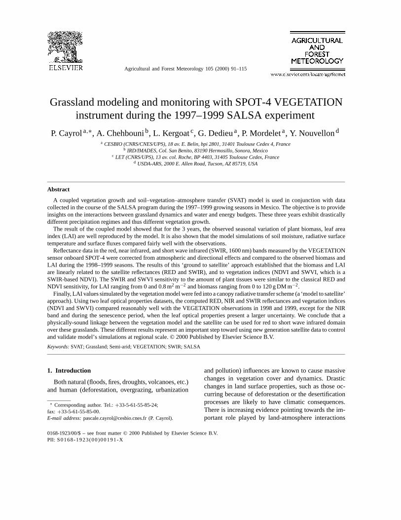
Fig. 5. (a) Simulated (–) and observed (d) hourly latent and sensible heat fluxes for a 20-day period of the 1997 growing season; (b)average diurnal cycle (local solar time) of the difference between measured and simulated components of the energy budget for the 1997and 1998 growing seasons. Net radiation (–·), soil heat flux (· · ·), latent heat flux (–) and sensible heat flux (– –). Measurements of sensibleand latent heat fluxes were not available for 1998.

the maximum biomass were different in 1997 whencompared to 1998 and 1999. This is due to differencesin both the amount and the temporal distribution ofthe rainfall. Fig. 3 presents a comparison between ob-served and simulated LAI. The LAI simulated by theV–S model agrees well with the measurements, al-though the comparison is meaningless for 1997 due to


Fig. 5 (Continued)

the short observation period. Maximum LAI was 0.32in 1997, but it reached 0.4 in 1998 and 0.75 in 1999.

Fig. 4 focuses on a 20-day period (day of year246–265), and shows the dynamics of the simulatedand observed hourly values (half hourly for 1999) ofsoil moisture in the root zone (w2) for all three studyyears. This period corresponds to the end of the rainseason, and the grasses are usually at maximum de-velopment. The simulated soil moisture is within therange of TDR measurements, except for DoY 246–255in 1998, when soil moisture is overestimated. This ismainly the result of model’s errors, which occur ear-lier in 1998 (the simulation starts at DoY 171 for thisyear). Such discrepancies were inherent to the use ofthe same set of parameters (soil resistance, field ca-pacity). This gives a reasonable agreement for the 3years, although a year to year re-calibration can pro-duce better but less robust results. The 20-day periodcorresponds to a dry spell in 1999, although the simu-lated soil moisture is much higher than in 1997 whenaveraged over the whole growing season.

The time series of the simulated versus observedlatent and sensible heat fluxes are shown in Fig. 5a forthe same period of time. The root mean square error

(RMSE) between measured and simulated latent andsensible heat fluxes were 36 and 38 W m−2, respec-tively and therefore in good agreement. On Fig. 5b,we have represented the average diurnal cycle of thedifference between the observed and estimated com-ponents of the energy balance for 1997 and 1998.There is a systematic bias around 11.00 h (LST) withan overestimation of the simulated latent and sensibleheat fluxes. Given the errors associated with surfaceflux measurements in semi-arid regions, and the qual-ity of the energy balance closure, this bias is relativelysmall.

Fig. 6a–c present comparison of daytime (7.00 hto 20.00 h) measured and simulated radiative surfacetemperature (DoY 246–265) in 1997–1999, respec-tively. The results for the 3 years are rather similar.There is a slight underestimation of the radiative sur-face temperature for the highest values (>50◦C), butthe correlations for the whole range of data are strong.

There is still room for validation. For instance, theallocation of carbon to the roots, as well as the parti-tion between soil evaporation and plant transpirationwere not measured and validated. Moreover, the sim-ulations also reflect the uncertainties in some critical


Fig. 6. (a) Simulated radiative temperature vs. ground-based observations at nadir for year 1997, (hourly data, DoY 246–265). The (1:1)line and the correlation coefficient (r) are indicated; (b) same as Fig. 6a, but for year 1998 (DoY 246–265); (c) simulated radiativetemperature vs. ground-based observations at nadir for 1999 (half-hourly data, DoY 246–265).


Fig. 6 (Continued)

parameters, as highlighted by Cayrol et al. (in press).Nevertheless, the previous evaluations show that themain features of the water and carbon dynamics areproperly reproduced by the V–S model, which cap-tures the variability of plant response to the climatevariability.

5. Ground and satellite data

The objective of this section is to assess the capabil-ity of the SPOT4-VEGETATION and NOAA/AVHRRsensors to track the temporal evolution of the vegeta-tion, and to address the questions 3 and 4 mentionedin Section 1.

Both ground measurements and model results pre-sented in the previous section indicate that the LAI ofthe Zapata grassland site is low (less than 0.8), andstrongly variable over the timeframe of the study. Be-fore exploiting the coupling of remotely sensed dataand models, we need to verify whether the seasonalevolution as well as the year to year variability of thevegetation is captured by satellite observations, evenfor such a low vegetation cover.

5.1. Ground-to-satellite approach

Fig. 7a–c present the temporal variations of AVHRRand VEGETATION NDVI for the 1997–1999 grow-ing seasons, respectively. The AVHRR NDVI signalin 1997 is almost flat, with a small and late peaknear DoY 285, whereas it increases much earlier andreaches higher values in 1998. In 1998, VEGETA-TION and AVHRR-based NDVI show consistent pat-terns. These two NDVI time series are not expected tomatch, because of differences in the spectral bands, in-strument field of view and data processing. In 1998 and1999, the time profiles show similar patterns, with amuch more pronounced peak in 1999, which is qualita-tively consistent with the biomass data in Figs. 1 and 3.

Fig. 8 presents the seasonal variations of VEGETA-TION-based surface reflectance during the 1999season. The strong day-to-day variations reflect thechanges in the sun-sensor-target geometry, whichaffect anisotropic surfaces. In order to compare thesurface reflectance to vegetation biophysical proper-ties, these directional effects have been removed, asdetailed in Appendix A. This correction minimizesthe short term variations and retains the seasonal


Fig. 7. NDVI time profile over the Zapata grassland, obtained from AVHRR (+) during (a) 1997 and (b) 1998 and from VEGETATION(s) during (b) 1998 and (c) 1999.

evolution. It is the latter corrected surface reflectances,which are used in the subsequent discussion.

The main objective in grassland monitoring is toestimate the evolution with time of the biomass usingsatellite data as surrogate measures. Scatter plots ofLAI and biomass versus the SWIR and the RED re-flectance (Fig. 9a and b) reveal significant linear rela-tionships (Table 3). It is well-known that the green leaf

pigments absorb in the red wavelength and that the leafwater absorbs in the SWIR wavelength (e.g. Hunt andRock, 1989). The figures establish that such relation-ships are still valid at the satellite and canopy level.This result had still to be demonstrated for the SWIRband. The correlation coefficient of the SWIR/biomass(SWIR/LAI, respectively) isr = −0.63 (r = −0.68)whereas it is−0.74 (−0.76) for the RED band. The


Fig. 8. Summertime reflectance (SWIR, NIR and RED reflectances) acquired by the VEGETATION sensor over the Zapata grassland in1999. Bold symbols represent reflectances after correction for surface anisotropy effects.

scattering is partly caused by the residual noise, whichstill impairs the satellite time series. This noise seemsto be larger for the SWIR than for the RED band(Fig. 8), and this may be related to the SWIR absorp-tion by the superficial soil moisture during the rainseason (DoY 200–250). Another slight difference isthat the RED reflectance increases gradually duringthe senescence period (270–320) whereas the SWIRincreases more rapidly and plateaus around DoY 290.

Whether this is related to a different timing in leaf‘drying’ and leaf ‘yellowing’ remains unclear at thisstage. When the reflectances are combined into vege-tation indices, the correlation improved (Fig. 9c) andreachedr = 0.81 (r = 0.88, respectively) for theNDVI/biomass (NDVI/LAI) andr = 0.76 (r = 0.86)for the SWVI/biomass (SWVI/LAI, respectively). Theresults are slightly better when the satellite data ac-quired during senescence are excluded (black symbols


Fig. 9. Scatter diagrams of the SWIR reflectance acquired by the VEGETATION sensor vs. the measured aboveground biomass and LAIduring the two growing seasons (s), (e) and senescence periods (d), (r) of 1998 and 1999, respectively. The linear regressions arealso plotted. Daily ’measurements’ of biomass and LAI are linearly interpolated from Figs. 1 and 3; (b) as in Fig. 9a except for the REDreflectance; (c) as in Fig. 9a except for the SWVI and NDVI vegetation indices.

in Fig. 9a–c). Not surprisingly, the regression are bet-ter for the LAI than for the biomass.

As far as we know, few studies, if any, have relatedthe seasonal evolution of satellite-measured SWVI andvegetation characteristics, simply because the previ-ous AVHRR sensor did not record the reflectance inthe SWIR (AVHRR channel 3 is also sensitive to thethermal emission). While these results are empirical,they are of interest since the impact on aerosol opti-cal depth is much smaller on the SWIR spectral band

than on the RED one. Since both wavelengths are sen-sitive to LAI, it is likely that a combined use of theSWIR, NIR and RED, also available on MODIS, maybe more accurate than the former NIR and RED bandsalone for vegetation monitoring.

5.2. Model-to-satellite approach

Finally, LAI values simulated by the model wereused as input to a canopy radiative transfer model


Fig. 9 (Continued)

Table 3Correlations, slopes and intercepts of the linear relationships between VEGETATION reflectances (SWIR and RED), vegetation indices(SWVI and NDVI) and measured biomass and LAI collected over two years (1998 and 1999)

Biomass (g DM m−2)a LAI (m2 m−2)a

SWIR −0.63 −0.68−0.0005, 0.3048 −0.0755, 0.3046

RED −0.74 −0.76−0.0005, 0.1586 −0.0677, 0.1572

NDVI 0.81 0.880.0026, 0.1505 0.3780, 0.1485

SWVI 0.76 0.860.0019,−0.1757 0.2991,−0.1832

a Correlation coefficient (r), slope and intercept of linear relationships.


(scattering by arbitrarily inclined leaves (SAIL); Ver-hoef, 1984) to compute surface reflectance in RED,NIR and SWIR regions (see Appendix C for moredetails). The central assumption is that the canopyreflectance depends on variables, green LAI, deadLAI, and can be computed by using SAIL and a set of

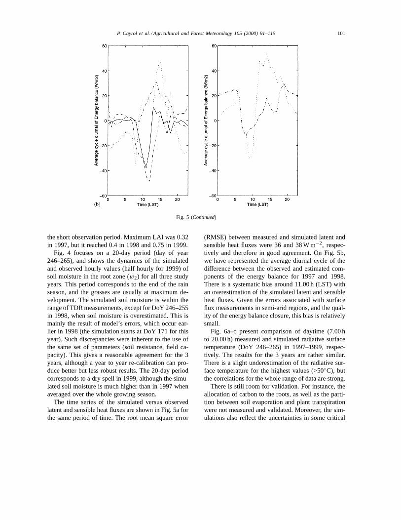
Fig. 10. (a) Comparison of the RED, NIR and SWIR reflectances simulated with the SAIL+V–S model and the normalized VEGETATIONreflectances (s) over the Zapata grassland site in 1998 (the three figures on the left) and in 1999 (the three figures on the right). Simulationswith the leaf optical properties from Walter-Shea et al. (1992) are in dashed line and solid line represents the simulation with the leafoptical properties from Asner et al. (1998); dotted lines are for the ’bright’ and ’dark’ parameter sets, see text); (b) as in Fig. 10a exceptfor the vegetation indices, SWVI (s) and NDVI (+).

fixed parameters such as the green and yellow opticalproperties, the leaf angle distribution. Two litera-ture datasets provided leaf optical properties for thegrasses found on the Zapata site or for closely relatedspecies: Asner et al. (1998) and Walter-Shea et al.(1992) (see Table 4). The soil reflectance were derived


Fig. 10 (Continued)

from springtime VEGETATION data. Simulationserrors were assessed by deriving a set of ‘bright’ opti-cal properties for green, yellow leaves and soil, and aset of ‘dark’ properties using the standard deviations(Tables 4 and 5). Fig. 10a presents the comparisonbetween simulated and observed reflectances (RED,NIR and SWIR). For each wavelengths, one param-eter set or the other yielded a very good match tothe VEGETATION data. However, here is no generalagreement, because of the difference in the leaf opti-

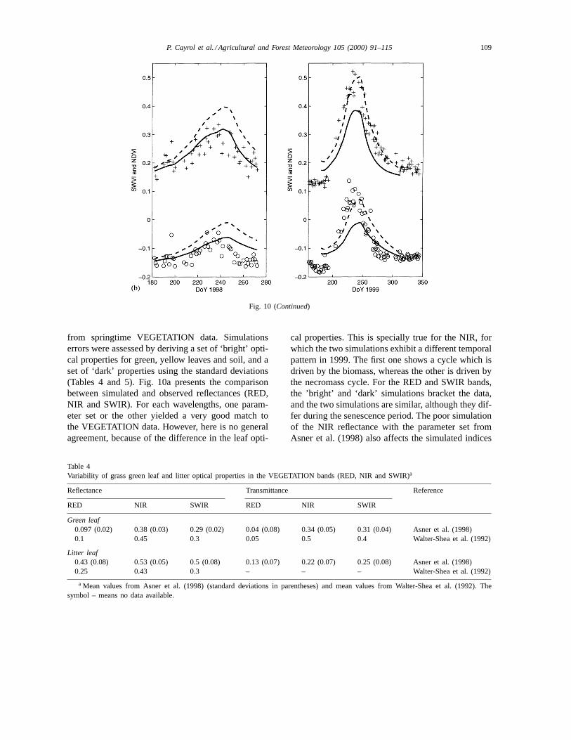
Table 4Variability of grass green leaf and litter optical properties in the VEGETATION bands (RED, NIR and SWIR)a

Reflectance Transmittance Reference

RED NIR SWIR RED NIR SWIR

Green leaf0.097 (0.02) 0.38 (0.03) 0.29 (0.02) 0.04 (0.08) 0.34 (0.05) 0.31 (0.04) Asner et al. (1998)0.1 0.45 0.3 0.05 0.5 0.4 Walter-Shea et al. (1992)

Litter leaf0.43 (0.08) 0.53 (0.05) 0.5 (0.08) 0.13 (0.07) 0.22 (0.07) 0.25 (0.08) Asner et al. (1998)0.25 0.43 0.3 – – – Walter-Shea et al. (1992)

a Mean values from Asner et al. (1998) (standard deviations in parentheses) and mean values from Walter-Shea et al. (1992). Thesymbol – means no data available.

cal properties. This is specially true for the NIR, forwhich the two simulations exhibit a different temporalpattern in 1999. The first one shows a cycle which isdriven by the biomass, whereas the other is driven bythe necromass cycle. For the RED and SWIR bands,the ’bright’ and ‘dark’ simulations bracket the data,and the two simulations are similar, although they dif-fer during the senescence period. The poor simulationof the NIR reflectance with the parameter set fromAsner et al. (1998) also affects the simulated indices


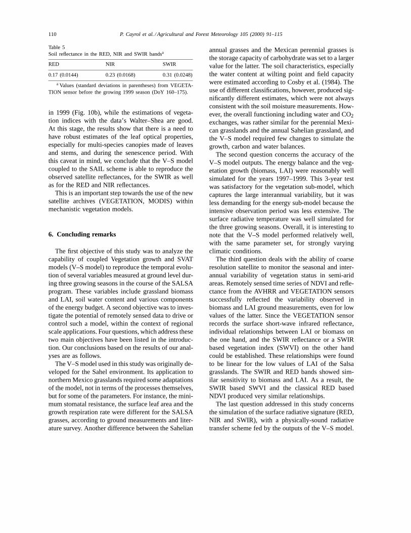
Table 5Soil reflectance in the RED, NIR and SWIR bandsa

RED NIR SWIR

0.17 (0.0144) 0.23 (0.0168) 0.31 (0.0248)

a Values (standard deviations in parentheses) from VEGETA-TION sensor before the growing 1999 season (DoY 160–175).

in 1999 (Fig. 10b), while the estimations of vegeta-tion indices with the data’s Walter–Shea are good.At this stage, the results show that there is a need tohave robust estimates of the leaf optical properties,especially for multi-species canopies made of leavesand stems, and during the senescence period. Withthis caveat in mind, we conclude that the V–S modelcoupled to the SAIL scheme is able to reproduce theobserved satellite reflectances, for the SWIR as wellas for the RED and NIR reflectances.

This is an important step towards the use of the newsatellite archives (VEGETATION, MODIS) withinmechanistic vegetation models.

6. Concluding remarks

The first objective of this study was to analyze thecapability of coupled Vegetation growth and SVATmodels (V–S model) to reproduce the temporal evolu-tion of several variables measured at ground level dur-ing three growing seasons in the course of the SALSAprogram. These variables include grassland biomassand LAI, soil water content and various componentsof the energy budget. A second objective was to inves-tigate the potential of remotely sensed data to drive orcontrol such a model, within the context of regionalscale applications. Four questions, which address thesetwo main objectives have been listed in the introduc-tion. Our conclusions based on the results of our anal-yses are as follows.

The V–S model used in this study was originally de-veloped for the Sahel environment. Its application tonorthern Mexico grasslands required some adaptationsof the model, not in terms of the processes themselves,but for some of the parameters. For instance, the mini-mum stomatal resistance, the surface leaf area and thegrowth respiration rate were different for the SALSAgrasses, according to ground measurements and liter-ature survey. Another difference between the Sahelian

annual grasses and the Mexican perennial grasses isthe storage capacity of carbohydrate was set to a largervalue for the latter. The soil characteristics, especiallythe water content at wilting point and field capacitywere estimated according to Cosby et al. (1984). Theuse of different classifications, however, produced sig-nificantly different estimates, which were not alwaysconsistent with the soil moisture measurements. How-ever, the overall functioning including water and CO2exchanges, was rather similar for the perennial Mexi-can grasslands and the annual Sahelian grassland, andthe V–S model required few changes to simulate thegrowth, carbon and water balances.

The second question concerns the accuracy of theV–S model outputs. The energy balance and the veg-etation growth (biomass, LAI) were reasonably wellsimulated for the years 1997–1999. This 3-year testwas satisfactory for the vegetation sub-model, whichcaptures the large interannual variability, but it wasless demanding for the energy sub-model because theintensive observation period was less extensive. Thesurface radiative temperature was well simulated forthe three growing seasons. Overall, it is interesting tonote that the V–S model performed relatively well,with the same parameter set, for strongly varyingclimatic conditions.

The third question deals with the ability of coarseresolution satellite to monitor the seasonal and inter-annual variability of vegetation status in semi-aridareas. Remotely sensed time series of NDVI and refle-ctance from the AVHRR and VEGETATION sensorssuccessfully reflected the variability observed inbiomass and LAI ground measurements, even for lowvalues of the latter. Since the VEGETATION sensorrecords the surface short-wave infrared reflectance,individual relationships between LAI or biomass onthe one hand, and the SWIR reflectance or a SWIRbased vegetation index (SWVI) on the other handcould be established. These relationships were foundto be linear for the low values of LAI of the Salsagrasslands. The SWIR and RED bands showed sim-ilar sensitivity to biomass and LAI. As a result, theSWIR based SWVI and the classical RED basedNDVI produced very similar relationships.

The last question addressed in this study concernsthe simulation of the surface radiative signature (RED,NIR and SWIR), with a physically-sound radiativetransfer scheme fed by the outputs of the V–S model.


The leaf optical properties were taken from two dif-ferent dataset. It was shown that the V–S modelcoupled to the SAIL scheme generally captures theseasonal evolution of the VEGETATION reflectancesand spectral indices. For every spectral band, at leastone of the input dataset lead to a good simulationof the observed satellite reflectance. However, uncer-tainties in the leaf optical properties, especially inthe green leaf absorption in the NIR and in the deadtissues properties, resulted in large uncertainties inthe NIR simulations. Robust estimates of the leaf,stems and litter parameters and of their variability aretherefore highly desirable for regional scale applica-tions (e.g. through the validation network of the newsensors like MODIS). From the answers to these dif-ferent questions, it is concluded that the V–S modelis suitable for long term modeling and monitoringof surface processes in arid and semi-arid areas.The physically-based model-to-satellite approach ispromising, and the SAIL scheme seems also to besuitable for the SWIR band. Because this spectral do-main is known to be less sensitive to most aerosols,the VEGETATION and MODIS datasets may give adifferent view of the terrestrial ecosystems. Furtherwork will consist in assimilating the satellite mea-surements at regional scales, with the objective of ob-taining accurate simulations of vegetation dynamicsand surface energy budget over a large area.

Acknowledgements

This work and participation in the SALSA experi-ment were made possible through the support of theEC VEGETATION Preparatory Program and a Ph.D.grant from French MESR (Ministère de l’Enseigne-ment Supérieur et de la Recherche). Additional sup-port was provided by CONACyT and EOS-Project(NAGW2425). Many thanks are due to the many peo-ple involved in the implementation of the experimentin Mexico: Dr. Gilles Boulet, Dr. Chris Watts, Dr. J.-P.Brunel, Julio Rodriguez, O. Hartogensis, Mario Jauriand Saturnino Garcia. We would also like to thankDr. Bruce Goff for helping us with the species identi-fication. Thanks also to G. Saint (CNES), CTIV andSPOT-image for helping us to access VEGETATIONdata. We are very grateful to Drs B. Berthelot and Ph.Maisongrande for processing of VEGETATION data

and to Dr. Malcolm Davidson for carefully reading themanuscript. The authors also express their deep grat-itude to the anonymous reviewers for their valuablecomments and critical remarks.

Appendix A. Correction of the surface anisotropy

To remove the effect of surface anisotropy, we com-puted a normalized reflectance (Rnorm) using Eq. (A.1)from Wu et al. (1995)

Rnorm(Ao) = R(Aobs) × F with

F = Rmod(Ao)

Rmod(Aobs)(A.1)

where Ao is the reference or standard sun-sensorgeometry (Table 6), Aobs is the actual sun-sensorgeometry andF is the factor, which removes the di-rectional effects explained by a BDRF model. TheBRDF model used is the AMBRALS model (Wanneret al., 1997) which is based on parameters kernel

Rmod = k0 + k1f1(Aobs) + k2f2(Aobs) (A.2)

where k0, k1 and k2 are free parameters obtainedfitting Rmod to the data,f1 and f2 are the kernels,which are analytical functions of the sun and sensorzenith and azimuth angles. The first kernel aims atreproducing the volume scattering. The second ker-nel estimates the surface scattering and is based ongeometrical approaches. We used the Ross-thick ker-nel with the Li-sparse kernel. The surface reflectancemay then computed for any sun-sensor geometry, e.g.

Table 6Specification of the SAIL model input parameters

Canopy structure parametersLAI As predicted by the

V–S modelLeaf angle distribution Spherical (mean leaf

angle= 57.30◦)

Illumination and view conditionsDiffuse fraction of solar radiation 20%

Reference sun-target-sensora

View zenith angles 30◦Solar zenith angles 30◦Relative azimuth 140◦

a Standard geometry condition of VEGETATION.


the reference geometry (Ao). To account for a sea-sonal variation of the canopy properties, we used a‘seasonal’ Ambral model

Rmod = Ka0 + (1 − K)a′0

+(Ka1 + (1 − K)a′1)f1(Aobs)

+(Ka2 + (1 − K)a′2)f2(Aobs) (A.3)

wherea0, a1, a2 are the parameters corresponding tothe ‘maximum vegetation season’ and thea′

0, a′1, a′

2are the parameters corresponding to the ‘minimumvegetation season’. TheK coefficient is the NDVI,scaled between 0 and 1. This linear model is fitted tothe 1998 and 1999 VEGETATION data and is usedto provide normalized seasonal reflectances.

Appendix B. The V–S model’s main equations

Symbols and parameters values are listed in Table 1.

B.1. Daily time-step

B.1.1. Carbon balanceThe dynamics of the three carbon compartments is

described by a set of three differential equations

dMs

dt= asPn − msMs − Rgs − ssMs (B.1)

dMr

dt= (1 − as) Pn − mrMr − Rgr − srMr (B.2)

dMn

dt= ssMs − dnMn (B.3)

Eq. (B.1) expresses that the daily carbon increment ofthe shoots is the result of the carbon gain, photosynthe-sis (Pn) minus carbon lost during plant maintenance(msMs) and plant growth respiration (Rgs) and carbonlosses due to senescencessMs. The carbon availablefor growth is partitioned between the shoot and rootsaccording to theas allocation coefficient. The rootsobey a similar equation Eq. (B.2), with a symmetricallocation coefficient (1−as).

The necromass dynamic depends on the differencebetween necromass production, which is equal to theshoot senescencessMs, and necromass decaysdnMn.

The LAI is computed from the shoots biomassand SLA according to a non-linear relationship that

accounts for the increasing importance of stemsand other non-leaf tissues at high levels of biomass(relationship estimated from measurements Nouvel-lon, 1999) by the expression

SLA = 0.0001[130.4

−332.5(1 − exp(−0.0031nbj))] (B.4)

where nbj is the number of day after the beginning ofthe growing season.

The carbon balance equations Eqs. (B.1)–(B.3) aresolved on a daily basis, where as the photosynthesis(Pn) is computed and accumulated on an hourly basis.Indeed, it depends on the stomatal resistance, whichis also involved in the SVAT model, and computed onan hourly (or half-hourly) basis.

B.1.2. Respiration and senescenceFollowing McCree (1970) and Amthor (1986,

1989) the total respiration consists of maintenanceand growth respiration. The maintenance respirationis proportional to the biomass and its rate (ms or mrin Eqs. (B.1) and (B.2)) depends on air temperatureaccording to a classicalQ10 relationship:

ms = ms0QT/1010 (B.5)

whereT is the daily average air temperature andms0 isthe respiration rate at 0◦C for the shoot (mr0 for roots,respectively). The growth respiration is proportionalto the amount of new tissue and therefore Eqs. (B.1)and (B.2) have to be rearranged as follows:

dMs

dt= 1

1 + gs(asPn − msMs) − ssMs (B.6)

dMr

dt= 1

1 + gr[(1 − as)Pn − mrMr] − srMr (B.7)

The dry matter is lost through the senescence of shootand root tissues Eqs. (B.6) and (B.7). We consideredhere a normal senescence ratess0 (sr0 for roots, respec-tively) and a water stress effect that increases senes-cence

ssMs = ss0

[1 +

(1 − w2 − wwp

wfc − wwp

)]Ms (B.8)


B.2. Hourly (or half hourly) time step

B.2.1. Stomatal resistanceThe leaf stomatal resistance is of Jarvis’s (1976)

type

rs = rs minf (I)g(W)h(vpd)

= rs min

(Is + I

I

) (wfc − wwp

w2 − wwp

) (4000− 1000

4000− vpd

)(B.9)

B.2.2. PhotosynthesisAt leaf level,Pl = (Ca−Γ )/(r

CO2s +rr) whererCO2

sand rr are the stomatal and residual resistances (i.e.mesophyll diffusion and carboxylation resistances) toCO2 transfer (e.g. Running and Coughlan, 1988). SeeCayrol et al. (in press) for parameters derivations.

rr = rr min g1(I )g2(T )

= rr minIr + I

I

(Tmax − Tmin)2

4(Tmax − T )(T − Tmin)(B.10a)

At the canopy level, Pc = τ(Ca− Γ )

ke(r ′s + r ′

r)ln

×(

r ′sIs + r ′

rIr + keI0(r′s + r ′

r)

r ′sIs + r ′

rIr + keI0(r ′s + r ′

r) exp(−keLAI )

)(B.10b)

where r ′s is for rs ming(W)h(vpd) and r ′

r is forrr ming2(T).

B.2.3. Prognostic equations, surface fluxes andradiative temperature

The equations giving the evolution of the prognosticvariables are

∂Tg

∂t= 2π1/2G

(cgλgτ)1/2− 2π

τ(Tg − T2) (B.11)

∂T2

∂t= G

(356cgλ2τ)1/2(B.12)

∂wg

∂t= C1

ρwd1(P − Eg) − C2

τ(wg − weq),

0 ≤ wg ≤ wsat (B.13)

∂w2

∂t= 1

ρwd2(P − Eg − Etr)

− C3

d2τmax [0, (w2 − wfc)], 0 ≤ w2 ≤ wsat

(B.14)

The energy balance is written separately for the soiland vegetation

Rng − LEg − Hg − G = 0 (B.15)

and

Rnc − LEc − Hc = 0 (B.16)

The network of resistances from Shuttleworthand Wallace (1985), between the soil surface, thewithin-canopy source level and the above-canopy ref-erence level allows to estimate the latent and sensibleheat fluxes across differences in vapor pressure andtemperature given by

LE = ρCp

γ

(e0 − ea

raa

)(B.17)

H = ρCp(T0 − Ta)

raa(B.18)

for the soil components

LEg = ρCp

γ

(esat(Tg) − e0

ras+ rss

)(B.19)

Hg = ρCp(Tg − T0)

ras(B.20)

for the vegetation components

LEc = ρCp

γ

(esat(Tc) − e0

rac + rsc

)(B.21)

Hc = ρCp(Tc − T0)

rac(B.22)

The radiative temperature is expressed as follows:

Tr =[(RA − RAc − RAg)

σ

]0.25

(B.23)

Appendix C. The SAIL model

SAIL is a turbid medium reflectance model,which considers a homogeneous canopy and uses the


Kubelka–Munk approximation to the radiative trans-fer equation (Goel, 1988). The model simulates thecanopy spectral reflectance from LAI, leaf and soiloptical properties, leaf angle distribution, acquisitiongeometry and diffuse part of the incoming solar radia-tion. The ratio between leaf size and vegetation heightaccounts for the hot-spot effect. The green and yellowLAI were predicted daily by the V–S model. The ge-ometric conditions correspond to the acquisition con-figurations (Table 6). The soil reflectances for visible,near infrared and short wave infrared were estimatedfrom the first images of VEGETATION sensor beforethe beginning of the growing season (Table 5). Leafoptical parameters (Table 4) were prescribed for visi-ble, near infrared and short wave infrared from Asneret al. (1998) and Walter-Shea et al. (1992). A versionof the SAIL model with two layers was used. Greenvegetation was assumed to overtop dead leaves.

References

Amthor, J.S., 1986. Evolution and applicability of a whole plantrespiration model. J. Theoritical Biol. 122, 473–490.

Amthor, J.S., 1989. Respiration and Crop Productivity. Springer,New York.

Asner, G.P., Wessman, C.A., Schimel, D.S., Archer, S., 1998.Variability in leaf and litter optical properties: implications forBRDF model inversion using AVHRR, MODIS and MISR,MODIS and MISR. Remote Sens. Environ. 63, 243–257.

Avissar, R., 1995. Recent advances in the presentation of land-atmosphere interactions in general circulation models. Rev.Geophys. 2, 1005–1010.

Bonan, G.B., Pollard, D., Thompson, S.L., 1992. Effects of borealforest vegetation on global climate. Nature 359, 716–718.

Braud, I., Noilhan, J., Bessemoulin, P., Haverkamp, R., Vauclin,M., 1993. Bare-ground surface heat and water exchanges underdry conditions: observations and parameterization. BoundaryLayer Meteorol. 66, 173–200.

Calvet, J.C., Noilhan, J., Rougean, J.L., Bessemoulin, P.,Cabelguenne, M., Olioso, A., Wigneron, J.P., 1998a. An interac-tive vegetation SVAT model tested against data from sixcontrasting sites. Agric. For. Meteorol. 92, 73–95.

Calvet, J.C., Noilhan, J., Bessemoulin, P., 1998b. Retrieving theroot-zone soil moisture or temperature estimates: a feasibilitystudy based on field measurements. J. Appl. Meteorol. 37, 371–386.

Cayrol, P., Kergoat, L., Moulin, S., Dedieu, G., Chehbouni, A.,Calibrating a coupled SVAT/vegetation growth model withremotely sensed reflectance and surface temperature. A casestudy for the HAPEX-Sahel grassland sites. J. Appl. Meteorol.,in press.

Chanzy, A., 1991. Modelisation simplifiée de l’évaporation d’un solnu utilisant l’humidité et la temperature de surface accessibles

par télédétection. Thèse de docteur ingénieur agronome del’Institut National Agronomique Paris-Grignon, France, p. 221.

Choudhury, B.J., Monteith, J.L., 1988. A four layer model for theheat budget of homogeneous land surfaces. Q.J.R. Met. Soc.114, 373–398.

Clapp, R.B., Hornberger, G.M., 1978. Empirical equations for somesoil hydraulic properties. Water Resour. Res. 14 (4), 601–604.

Cosby, B.J., Hornberger, G.M., Clapp, R.B., Ginn, T.R., 1984.A statistical exploration of the relationships of soil moisturecharacteristics to the physical properties of soils. Water Resour.Res. 20, 682–690.

Deardorff, J.W., 1978. Efficient prediction of ground surface temp-erature and moisture, with inclusion of a layer of vegetation.J. Geophys. Res. 83, 1889–1903.

DeVries, D.A., 1963. Thermal properties of soils. In: Van Wijk,N.R. (Ed.), Physics of Plant Environment. Holland Publishing,Amsterdam.

Dickinson, R.E., Shaikh, M., Bryant, R., Graumlich, L., 1998.Interactive canopies for a climate model. J. Climate 11, 2823–2836.

Giordani, H., Noilhan, J., Lacarrère, J., Bessemoulin, P., 1996.Modeling the surface processes and the atmospheric boundarylayer for semi-arid conditions. Agric. For. Meteorol. 80, 263–287.

Goel, N.S., 1988. Models of vegetation canopy reflectance and theiruse in estimation of biophysical parameters from reflectancedata. Remote Sens. Rev. 4, 1–212.

Goodrich, D.C., Chehbouni, A., Goff, B., MacNish, B., MaddockIII, T., Moran, M.S., Shuttleworth, W.J., Williams, D.G.,Watts, C., Hipps, L.H., Cooper, D.I., Schieldge, J., Kerr, Y.H.,Arias, H., Kirkland, M., Carlos, R., Cayrol, P., Kepner, W.,Jones, B., Avissar, R., Begue, A., Bonnefond, J.-M., Boulet,G., Branan, B., Brunel, J.P., Chen, L.C., Clarke, T., Davis,M.R., DeBruin, H., Dedieu, G., Elguero, E., Eichinger, W.E.,Everitt, J., Garatuza-Payan, J., Gempko, Gupta, H., Harlow, C.,Hartogensis, O., Helfert, M., Holifield, C., Hymer, D., Kahle,A., Keefer, T., Krishnamoorthy, S., Lhomme, J.-P., Lagouarde,J.-P., Lo Seen, D., Laquet, D., Marsett, R., Monteny, B., Ni,W., Nouvellon, Y., Pinker, R.T., Peters, C., Pool, D., Qi, J.,Rambal, S., Rodriguez, J., Santiago, F., Sano, E., Schaeffer,S.M., Schulte, S., Scott, R., Shao, X., Snyder, K.A., Sorooshian,S., Unkrich, C.L., Whitaker, M., Yucel, I., 2000. Preface paperto the semi-arid land-surface-atmosphere (SALSA) programspecial issue. Agric. For. Meteorol. 105, 3–19.

Gupta, H.V., Sorooshian, S., Yapo, P.O., 1998. Towardimproved calibration of hydrologic models: multiple and noncommensurable measures of information. Water Resour. Res.34 (4), 751–763.

Hunt Jr., E.R., Rock, B.N., 1989. Detection of changes in leafwater content using near- and middle-infrared reflectances.Remote Sens. Environ. 30, 43–54.

Jarvis, P.G., 1976. The interpretation of the variations in the leafwater potential and stomatal conductance found in canopies inthe field. Phil. Trans. R. Soc. London, Ser. B 273, 593–610.

Kergoat, L., 1998. A model for hydrological equilibrium of leafarea index on a global scale. J. Hydrol. 212/213, 268–286.

Kustas, W.P., Prueger, J.H., Humes, K.S., Starks, P.J., 1999.Estimation of surface heat fluxes at field scale using surface


layer versus mixed-layer atmospheric variables with radiometrictemperature observations. J. Appl. Meterol. 38, 224–238.

Le Roux, X., 1995. Etude et modélisation des échanges d’eau etd’énergie sol-végétation-atmosphére dans une savane humide(Lamto, Côte d’Ivoire). Thèse de l’université Pierre et MarieCurie, Paris, France, p. 203.

Lo Seen, D., Chehbouni, A., Njoku, E.G., Saatchi, S., Mougin, E.,Monteny, B., 1997. A coupled biomass production, water andsurface energy balance model for remote sensing applicationin semiarid grasslands. Agric. For. Meteorol. 83, 49–74.

Mahfouf, J.F., Noilhan, J., 1996. Inclusion of gravitational drainagein a land surface scheme based on the force-restore method. J.Appl. Meteorol. 35 (6), 987–992.

Mahrt, L., Ek, M., 1984. The influence of atmospheric stabilityon potential evaporation. J. Clim. Appl. Meteorol. 23, 222–234.

McCree, K.J., 1970. An equation for the rate of respiration ofwhite clover plants grown under controlled conditions. In:Setlik, I. (Ed.), Prediction and Measurement of PhotosyntheticProductivity. Proceedings of the IBP/PP Technical Meeting,Trebon, PUDOC, Wageningen, The Netherlands, pp. 221–229.

Nobre, C.A., Sellers, P.J., Shukla, J.U., 1991. Amazonian defo-restation and regional climate change. J. Climate 4, 957–987.

Nouvellon, Y., 1999. Modélisation du fonctionnement de prairiessemi-arides et assimilation de données radiométriques dans lemodèle. Thèse de docteur ingénieur agronome de l’InstitutNational Agronomique Paris, France.

Nouvellon, Y., Rambal, S., Lo Seen, D., Moran, M.S., Lhomme,J.P., Bégué, A., Chehbouni, A.G., Kerr, Y., 2000. Modellingof daily fluxes of water and carbon from shortgrass steppes.Agric. For. Meteor. 100, 137–153.

Passerat de Silans, A., 1986. Transferts de masse et de chaleur dansun sol stratifié soumis à une exitation atmosphérique naturelle.Comparaison modèle expérience, Thèse de l’institut Nationalde Polytechnique de Grenoble, France, 205 p.

Pielke, R.A., Liston, G.E., Lu, L., Vidale, P.L., Walko, R.L., Kittel,T.G.F., Parton, W.J., Field, C.B., 1997. Coupling of land andatmospheric models over the GCIP area — CENTURY, RAMS,and SIB2C, 2–7 February 1997, LongBeach, CA (preprint ofthe 13th Conference on Hydrology).

Running, S.W., Coughlan, J.C., 1988. A global model of forestecosystem processes for regional applications. Hydrologicalbalance canopy gas exchange and primary production processes.Ecol. Model. 42, 125–154.

Schmugge, T.J., 1980. Effect of texture on microwave emissionfrom soils. IEEE Trans. Geosci. Rem. Sensing, GE 18 (4),353–361.

Shuttleworth, W.J., Gurney, R.J., 1990. Evaporation from sparsecrops — an energy combination theory. Q.J.R. Met. Soc. 111,839–855.

Shuttleworth, W.J., Wallace, J.S., 1985. The theoretical relation-ships between foliage temperature and canopy resistance insparse crops. Q.J.R. Met. Soc. 116, 497–519.

Stannard, D.I., Blanfort, J.H., Kustas, W.P., Nichols, W.D., Amer,S.A., Shummge, T.J., Weltz, M.A., 1994. Interpretation ofsurface flux measurements in heterogeneous terrain during theMonsoon’90 experiment. Water Resour. Res. 30, 1227–1239.

Van de Griend, A.A., O’Neill, P.E., 1986. Discrimination of soilhydraulic properties by combined thermal infrared and micro-wave remote sensing. In: Proceedings of the IGARSS’86 Sym-posium, Vol. 254, Zurich, 8–11 September 1986. ESA SP,pp. 839–845.

Verhoef, W., 1984. Light scattering by leaf layers with applicationto canopy reflectance modeling: the SAIL model. Remote Sens.Environ. 16, 125–141.

Walter-Shea, E.A., Blad, B.L., Hays, C.J., Mesarch, M.A., 1992.Biophysical properties affecting vegetation canopy reflectanceand absorbed photosynthetically active radiation at the FIFEsite. J. Geophys. Res. 97 (D17), 18925–18934.

Wanner, W., Strahler, A.H., Hu, B., Muller, J.P., Li, X., BarkerSchaaf, C.L., Barnsley, M.J., 1997. Global retrieval of bidirec-tional reflectance and albedo over land from EOS MODISand MISR data: theory and algorithm. J. Geophys. Res. 102,17143–17161.

Williams, G.J., Markley, J.L., 1973. The photosynthetic pathwaytype of North American shortgrass prairie species and someecological implications. Photosynthetica 7 (3), 262–270.

Wu, A., Li, Z., Cilhar, J., 1995. Effects of land cover typeand greeness on advanced very high resolution radiometerbidirectional reflectance: analysis and removal. J. Geophys. Res.100, 9179–9192.

grassland modeling and monitoring with spot-4 ......agricultural and forest meteorology 105 (2000)...

Documents