graph theory topics in computer networkingcms.uhd.edu/faculty/redlt/chadseniorproject.pdf · graph...

Graph Theory Topics in Computer

Networking

By Chad Hart

Spring 2013

In Partial Fulfillment of

Math 4395 - Senior Project

Department of Computer and Mathematical Sciences

Faculty Advisor:

Dr. Timothy Redl: _________________________________

Committee Member:

Dr. Volodymyr Hrynkiv: _________________________________

Committee Member:

Dr. Shishen Xie: _________________________________

Department Chairman:

Dr. Shishen Xie _________________________________

Graph Theory Topics in Computer Networking | Chad Hart 2

Abstract

This project analyzes which computer routing protocol performs the most efficiently. Each

protocol is built around a single source shortest path algorithm. We use MATLAB to construct

complex scenarios and determine which algorithms are best for graphs of variable lengths.


Table of Contents

Abstract ......................................................................................................................................................... 2

Chapter 1 – Introduction .............................................................................................................................. 5

Chapter 2 – History ....................................................................................................................................... 9

Chapter 3 – Shortest Path Algorithms ........................................................................................................ 13

Chapter 4 – Implementation and Experimental Data ................................................................................. 18

Chapter 5 – Conclusion ............................................................................................................................... 24

References .................................................................................................................................................. 26

Appendix A .................................................................................................................................................. 27


Table of Figures

Figure 1-1: Example of Undirected Graph ...................................................................................... 5

Figure 1-2: Example of Directed Graph .......................................................................................... 5

Figure 2-1: Navigation Software Example ...................................................................................... 9

Figure 2-2: Basic network using RIP .............................................................................................. 11

Figure 2-3: Basic network using OSPF ........................................................................................... 12

Figure 3-1: Network vertices with edges and weights ................................................................. 14

Figure 3-2: Pseudo-code for Dijkstra’s Algorithm ......................................................................... 15

Figure 3-3: Pseudo-code for Bellman-Ford Algorithm .................................................................. 17

Figure 4-1: Representation of matrix G ........................................................................................ 18

Figure 4-2: MATLAB code for buildMatrix() ............................................................................. 19-20

Figure 4-3: Complete or fully-meshed graph ................................................................................ 21

Figure 4-4: Runtime results for Dijkstra vs. Bellman-Ford (1 to 450 vertices) ............................. 22

Figure 4-5: Runtime results for Dijkstra vs. Bellman-Ford (1 to 700 vertices) ............................. 23

Figure A-1: MATLAB code for Brute-Force Algorithm .................................................................. 27

Figure A-2: MATLAB code for Dijkstra’s Algorithm ....................................................................... 28

Figure A-3: MATLAB code for Bellman-Ford Algorithm ................................................................ 30

Figure A-4: MATLAB code for driver.m: Example of Directed Graph ........................................... 32


Chapter 1 – Introduction

Have you ever wondered how your mail gets from your mailbox to another address?

Perhaps you are fascinated with how internet traffic travels from one country to the next.

Networks have been used in a variety of applications for hundreds of years. In the scope of

mathematics, we can visually depict these networks better through graphs. A graph is a

representation of a group or set of objects, called vertices, in which some of the vertices are

connected by links, also known as edges. The study of these graphs is often referred to as

Graph Theory. Figures 1-1 and 1-2 are examples of simple graphs.

The example used in Figure 1-1 is known as an undirected graph, a graph in which the

edges have no orientation. A more practical example of an undirected graph would be two

people shaking hands. Person A is shaking hands with person B and at the same time, person B

is shaking hands with person A. Figure 1-2 shows a directed graph, or digraph. A digraph has

edges that have direction and are called arcs. Arrows on the arcs are used to show the flow

from one node to another. For example, from Figure 1-2, vertex a can move to vertex b, but b

cannot move to b. Often times, graphs will be labeled with a number on the link between


nodes. This means that the graph is weighted and this number denotes the cost it takes to get

from one vertex to the next.

There are many topics being researched today related to Graph Theory. However, the

context of this paper will be focused on Shortest Path Algorithms (SPAs). More specifically, we

will discuss how SPAs are used in current computer networking technology. A shortest path

algorithm is a method that will find the best or least cost path from a given node to another

node. Two of the most common SPAs discussed in graph theory today are the Bellman-Ford

algorithm and Dijkstra’s algorithm.

Computer networking relies deeply on graph theory and shortest path algorithms.

Without SPAs, network traffic would have no direction and not know where to go. It also also

very important that network traffic does not loop. If a loop were to occur, data packets could

end up right back where they started. This is obviously very inefficient.

In our project, we will study various types of algorithms used in Interior Gateway

Protocols (IGPs). An Interior Gateway Protocol is a routing protocol that is used to share

routing information within a local Autonomous System (AS). Examples of these routing

protocols are Routing Information Protocol (RIP), Open Shortest Path First (OSPF) and Enhanced

Interior Gateway Routing Protocol (EIGRP). Each of these algorithms uses a unique method to

find shortest paths between network routes. Also, one of the most unique distinctions

between each routing protocol is how each chooses their edge weights. RIP considers the cost

from vertex to vertex to all be equal. Therefore, the shortest path is determined solely on the

shortest number of nodes used to get to the destination. OSPF uses a very simple calculation to


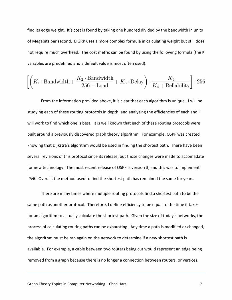
find its edge weight. It’s cost is found by taking one hundred divided by the bandwidth in units

of Megabits per second. EIGRP uses a more complex formula in calculating weight but still does

not require much overhead. The cost metric can be found by using the following formula (the K

variables are predefined and a default value is most often used).

From the information provided above, it is clear that each algorithm is unique. I will be

studying each of these routing protocols in depth, and analyzing the efficiencies of each and I

will work to find which one is best. It is well known that each of these routing protocols were

built around a previously discovered graph theory algorithm. For example, OSPF was created

knowing that Dijkstra’s algorithm would be used in finding the shortest path. There have been

several revisions of this protocol since its release, but those changes were made to accomadate

for new technology. The most recent release of OSPF is version 3, and this was to implement

IPv6. Overall, the method used to find the shortest path has remained the same for years.

There are many times where multiple routing protocols find a shortest path to be the

same path as another protocol. Therefore, I define efficiency to be equal to the time it takes

for an algorithm to actually calculate the shortest path. Given the size of today’s networks, the

process of calculating routing paths can be exhausting. Any time a path is modified or changed,

the algorithm must be ran again on the network to determine if a new shortest path is

available. For example, a cable between two routers being cut would represent an edge being

removed from a graph because there is no longer a connection between routers, or vertices.


Similarly, when a router is taken out of a network, this represents a vertex being removed from

the graph.

From past experience in computer networking, the arguments posed on choosing a

particular routing protocol are only related to which protocol is best for the type of equipment

or connections that are being used. I have not found any previous research to compare these

IGPs from a graph theory perspective.

It should also be known that this report will focus on undirected graphs. In the area of

computer networking, it is not practical to say that network traffic can flow in one direction

across a given path, but not the other direction. Therefore, directed graphs will be excluded

from most of the research topics.

Our report will begin with the history of SPA’s and computer networking and how they

were developed. Next, we will show our analysis of the shortest path algorithms. Then, we will

move in to the experimental portion and explain, in detail, how we used computer software to

find our results. Finally, we will unveil any improvements I have made to the routing protocols.


Chapter 2 – History

Shortest Path Algorithms are used in many applications of everyday life. Consider using

computer navigation software to obtain directions to a place you have never driven to before.

In most cases, there are many paths one could take in order to arrive at that location. This

software creates a graph with the vertices representing a physical location and the edges which

represent the road that connects two locations. If there is not a road between locations, then

there is not an edge in the graph. Next, a weight is associated with each edge. In this example,

the primary metric used for weight is distance. However, other factors in this example are

considered when assigning a weight, or cost, to an edge, such as traffic and average speed of

vehicles on a given road. Figure 2-1 shows an example of navigational software recommending

a path from one location to another. The shortest path, or the smallest sum of weights

between the two locations, is depicted by the dark blue line, while other alternate paths are

represented by the light blue lines.

Figure 2-1: Navigation Software Example


Path finding algorithms date back to the late 1800s. “Path finding, in particular

searching for a maze, belongs to the classical graph problems, and the classical references are

Wiener [1873], Lucas [1882], and Tarry [1895]. They form the basis for depth-first search

techniques.”1 However, it wasn’t until the 1950s that shortest path algorithm development

began to rise. This time period marked a new era of complex network applications. For

example, telephone networks were growing significantly larger, creating a demand for a more

efficient process to find the shortest path to the end caller. Before this period, call routing had

to be completed manually by telephone operators. Therefore, if a particular call path was

broken, it was not automatically intuitive as to which backup path should be taken. While

several mathematicians and computer scientists contributed to this research, two major

contributions were Edsger Dijkstra and Dijkstra’s algorithm in 1956 and also the Bellman-Ford

algorithm, developed by Lester Ford, Jr. and Richard Bellman in 1956 and 1958 respectively.

The Bellman-Ford algorithm was also published in 1957 by Edward F. Moore and is sometimes

referred to as the Bellman-Ford-Moore algorithm.

Computer networks began to evolve throughout the late 1950s and 1960s. The majority

of these networks were initially used in military operations for top secret data transfer and also

for radar system Semi-Automatic Ground Environment (SAGE)1. This created a great

opportunity for computer networking in the corporate world as well. American Airlines was the

first American company to fully utilize a complex network to connect mainframe systems for

the use of Semi-automated Business Research Environment (SABRE).


As corporate networks began to grow, it became very difficult to manually manage

every connection between sites. Configuring routers to direct traffic to a fixed location at all

times was completely inefficient. Routers needed the ability to dynamically calculate the best

and shortest path quickly. This process is referred to as dynamic routing.

The first major dynamic routing protocol, Routing Information Protocol (RIP), was

implemented in 1988. “This algorithm has been used for routing computations in computer

networks since the early days for the ARPANET” (RFC 1058). RIP runs as a software component

on routers based on the Bellman-Ford algorithm. Each routing protocol uses a different

method in calculating the cost between routers. RIP determines that the hop count is the

routing metric. Figure 2-2 shows that the metric between both A to B and B to C is 1.

Therefore, the total weight for the path from A to C is 2. RIP is still commonly used in networks

today.

Figure 2-2: Basic network using RIP

The second major dynamic routing protocol is called Open Shortest Path First (OSPF).

This protocol is current on version 2, which is defined by RFC 2328 and published by the

Internet Engineering Task Force (IETF) in 1998. Similarly, OSPF exercises a previously defined

shortest path algorithm, Dijkstra’s Algorithm. OSPF calculates determines the bandwidth

between two routers and then assigns that bandwidth amount in megabits per second to the

edge cost. For example, if the bandwidth between router A and B is 1 megabit (100 Mbps) and


the bandwidth between router B and C is 1 gigabit (1000 Mbps), the edge costs between the

routers will be 100 and 1000, respectively. This protocol is also implemented frequently in

corporate networks around the world today.

Figure 2-3: Basic network using OSPF


Chapter 3 – Shortest Path Algorithms

Now we will define each shortest path algorithm. Take a weighted digraph G = (V, E).

We denote the letter G as the name of the graph, V to be a representation of all the vertices in

the graph, and E to contain all the edges between vertices. Given a source and destination

vertex, it can be said that a sequential list of vertices in which connect the source and

destination can be called a path, where 𝑝 = 𝑣1 → 𝑣2 → ⋯ → 𝑣𝑘. The edge weights can be

given by a function 𝑤 ∶ 𝐸 → ℝ. Therefore, the weight can be written as follows:

𝑤(𝑝) = ∑ 𝑤(𝑣𝑖

𝑘−1

𝑖=1

, 𝑣𝑖+1)

After taking the sum of edges used for each path, the path that has the smallest sum can

be known as the shortest path. We can now define the shortest path weight to be 𝛿(𝑢, 𝑣) =

min {𝑤(𝑝): 𝑝𝑎𝑡ℎ 𝑓𝑟𝑜𝑚 𝑢 𝑡𝑜 𝑣}. A path can have an infinite cycle. However, if we choose an

algorithm that will not allow a vertex to be contained in a path more than once, then it will not

be infinite (assuming the graph contains a finite number of vertices).4

Before analyzing the frequently used shortest path algorithms, it is important to

examine the worst case scenario. This process of finding every applicable path in the graph,

and then finding the smallest sum of those edges in a particular path is known as the Brute-

Force algorithm.


Figure 3-1: Network vertices with edges and weights

From Figure 3-1 illustrates two possible paths from vertex A to D. Those paths are A-C-D

and A-B-C-D. The Brute-Force algorithm will first find all paths without considering the edge

weights. Once all paths are found, the algorithm will then find the shortest path. In simple

networks, there is not usually a problem with using the Brute-Force method. However, as the

graph grows larger, the Brute-Force requires many more computations.

Now, it will be helpful for us to look at the Single-Source Shortest Path algorithms.7

These are algorithms that from any given source vertex 𝑠 ∈ 𝑉 they will find the shortest path

𝛿(𝑠, 𝑣), ∀𝑣 ∈ 𝑉. To date, there is not an efficient algorithm that can find the shortest path from

one vertex to another specific vertex without taking into consideration the other vertices in the

graph.3 After the distance from the source to the other vertices has been calculated, it will be

easy to back track to find the path. Dijkstra’s Algorithm is the most common single-source

shortest path algorithm. It will require three inputs (G, w, s), the graph G (containing vertices

and edges, the weights w, and the source vertex s. Dijkstra’s Algorithm is outlined as follows:


𝑑𝑖𝑗𝑘𝑠𝑡𝑟𝑎 (𝐺, 𝑤, 𝑠)

𝑑[𝑠] = 0

𝑓𝑜𝑟 𝑒𝑎𝑐ℎ 𝑣 ∈ 𝑉 − {𝑠}

𝑑𝑜 𝑑[𝑣] = ∞

𝑆 = ∅

𝑄 = 𝑉

𝑤ℎ𝑖𝑙𝑒 𝑄 ≠ ∅

𝑑𝑜 𝑢 = 𝐸𝑥𝑡𝑟𝑎𝑐𝑡𝑀𝑖𝑛(𝑄)

𝑆 = 𝑆 ∪ {𝑢}

𝑓𝑜𝑟 𝑒𝑎𝑐ℎ 𝑣 ∈ 𝑎𝑑𝑗 {𝑢}

𝑑𝑜 𝑖𝑓 𝑑[𝑣] > 𝑑[𝑢] + 𝑤(𝑢, 𝑣)

𝑡ℎ𝑒𝑛 𝑑[𝑣] = 𝑑[𝑢] + 𝑤(𝑢, 𝑣)

Figure 3-2: Pseudo-code for Dijkstra’s Algorithm

Dijkstra’s algorithm must first initialize its three important arrays. First, the array S

contains the vertices that have already been examined or relaxed. It first starts as the empty

set, but as the algorithm progresses, it will fill it with each vertex until all are examined. Then,

the distance array d[x] is defined to be an array of the shortest paths from s to x, or also

denoted 𝛿(𝑠, 𝑥) 𝑤ℎ𝑒𝑛 𝑥 ∈ 𝑆. Finally, Q is simply the data type used to form the list of vertices.

In this case, we call it a priority queue.

Even though Dijkstra’s algorithm appears to be very efficient, it must only consider non

negative cost values on the edges, as having a negative value can result in an unwanted loop.

However, this is not an immediate concern from our study, because in each of our networking

protocols, there cannot be a negative metric value.


After the initialization portion of the algorithm is complete, we then move into the

shortest path calculation. The function will have to run as long as it takes to relax each edge for

each vertex. Next, we chose to use “ExtractMin” because we needed a method to choose a

new vertex to examine. Extracting the vertex corresponding to the least shortest path so far,

will guarantee choosing a new unique vertex. We must compare every edge that connects to

this newly chosen vertex u. If the adjacent vertex v currently has a distance to the source that

is greater than the distance to u plus the cost of the distance between u and v, then we must

update the distance to v.5 After completion of this step, we now have an array d[x] that holds

the value for the shortest distance for from the source to each of the vertices in the graph.

Chapter 4 will discuss how to traverse back through this array to list the vertices included in the

shortest path.

Now we will analyze Bellman-Ford algorithm, which can be seen below.


𝑏𝑒𝑙𝑙𝑚𝑎𝑛𝑓𝑜𝑟𝑑 (𝐺, 𝑤, 𝑠)

𝑑[𝑠] = 0

𝑓𝑜𝑟 𝑒𝑎𝑐ℎ 𝑣 ∈ 𝑉 − {𝑠}

𝑑𝑜 𝑑[𝑣] = ∞

𝑓𝑜𝑟 𝑖 = 1 𝑡𝑜 |𝑉| − 1

𝑑𝑜 𝑓𝑜𝑟 𝑒𝑎𝑐ℎ 𝑒𝑑𝑔𝑒 (𝑢, 𝑣) ∈ 𝐸

𝑑𝑜 𝑖𝑓 𝑑[𝑣] > 𝑑[𝑢] + 𝑤(𝑢, 𝑣)

𝑡ℎ𝑒𝑛 𝑑[𝑣] = 𝑑[𝑢] + 𝑤(𝑢, 𝑣)

Figure 3-3: Pseudo-code for Bellman-Ford Algorithm

The Bellman-Ford algorithm takes the same approach for initialization as Dijkstra. It will

also accept the graph to be input as a square matrix. Bellman-Ford is known to be fairly simple

but not run as efficiently. This shortest path algorithm will run be controlled by a “for-loop”

that runs |V| - 1 iterations where |V| is equal to the number of vertices in the network.

Bellman-Ford will now run the same relaxation test as Dijkstra for each edge in the graph.

Upon completion of each relaxation, the shortest path will be found.6 We can now move to the

experimental test where we can code these algorithms and test their results.


Chapter 4 – Implementation and Experimental Data

Before jumping into the analysis of these algorithms, it was important for us to choose a

mathematics software that best fit. MATLAB was chosen because it is matrix-oriented and

seemed to be the most efficient for making fast calculations.

In order to input data into the MATLAB functions, we had to have some sort of method

in which to describe the graphs. In previous sections, we were speaking generally with phrases

such as “for all edges” or “for each edge.” We chose to input the graph in the form of a square

matrix. The matrix will always be of n x n dimension where n is equal to the number of vertices

in the graph. Each row will represent the vertex from which we are traveling. Each column will

represent the vertex to which we are traveling to.2 The matrix G is a representation of the

graph with three vertices. Vertex A corresponds to row and column 1, B to row and column 2,

etc. Matrix G shown below is the matrix representation of the graph in Figure 4-1.

𝐺 = [0 1 21 0 32 3 0

]

Figure 4-1: Representation of matrix G


It can now be seen that the cost from A to B will correspond to row 1, column 2 in the

matrix. Therefore, 𝐺[1,2] is equal to 1, 𝐺[1,3] is equal to 2, and 𝐺[2,3] is equal to 3. Also note

that all of the elements in the diagonal of the matrix are equal to 0. This is a result of describing

the cost from one node to itself, which is clearly zero. Also, the matrix should be symmetric

across the diagonal. We decided earlier that our graphs should be undirected. The matrix

being symmetric would imply 𝑤(𝑥, 𝑦) = 𝑤(𝑦, 𝑥) 𝑤ℎ𝑒𝑛 ∀𝑥, 𝑦 ∈ 𝐺. If this were not the case,

then the graph would be directed.

The MATLAB functions are all run from a driver program called driver.m. This program

allows us to not have to enter each command manually. Given the amount of variables, the

driver function also allows us to not have to enter each variable for every call of the function.

Also, graphs with a very large number of vertices take a large amount of time to calculate. The

driver function allowed us to run multiple tests at one time with minimal time in between each

function call.

The next large task we faced was creating random graphs. We created a function

named buildMatrix() to build our graph. This function runs in 𝑂(𝑛2) time, where n equals the

number of nodes. For the sake of time calculations, we will leave this function out as it is

considered to be a premise of the problem.

function S = buildMatrix (sizeMatrix)

S = rand(sizeMatrix);

for (y = 1:sizeMatrix)

for (x = y:sizeMatrix)

if (x==y)


S(x,y) = 0;

else

if S(x,y)<=0.70

S(x,y) = 0;

end

S(y,x) = S(x,y);

end

end

end

Figure 4-2: MATLAB code for buildMatrix()

Initially, the function creates a n by n matrix with random numbers between 0 and 1 as

elements. Obviously, we do not want a completely random matrix. As previously discussed, we

need to have the elements on the diagonal of the matrix equal to zero. Also, the elements

need to follow the symmetric property previous discussed, 𝑤(𝑥, 𝑦) = 𝑤(𝑦, 𝑥). Therefore, the

“If-Then” command controlled by the nested loop analyses if the element is on the diagonal. If

it is, then the function sets that value equal to zero. If the element is not on the diagonal, it will

set the corresponding element on the other side of the diagonal such that 𝑤(𝑥, 𝑦) = 𝑤(𝑦, 𝑥).

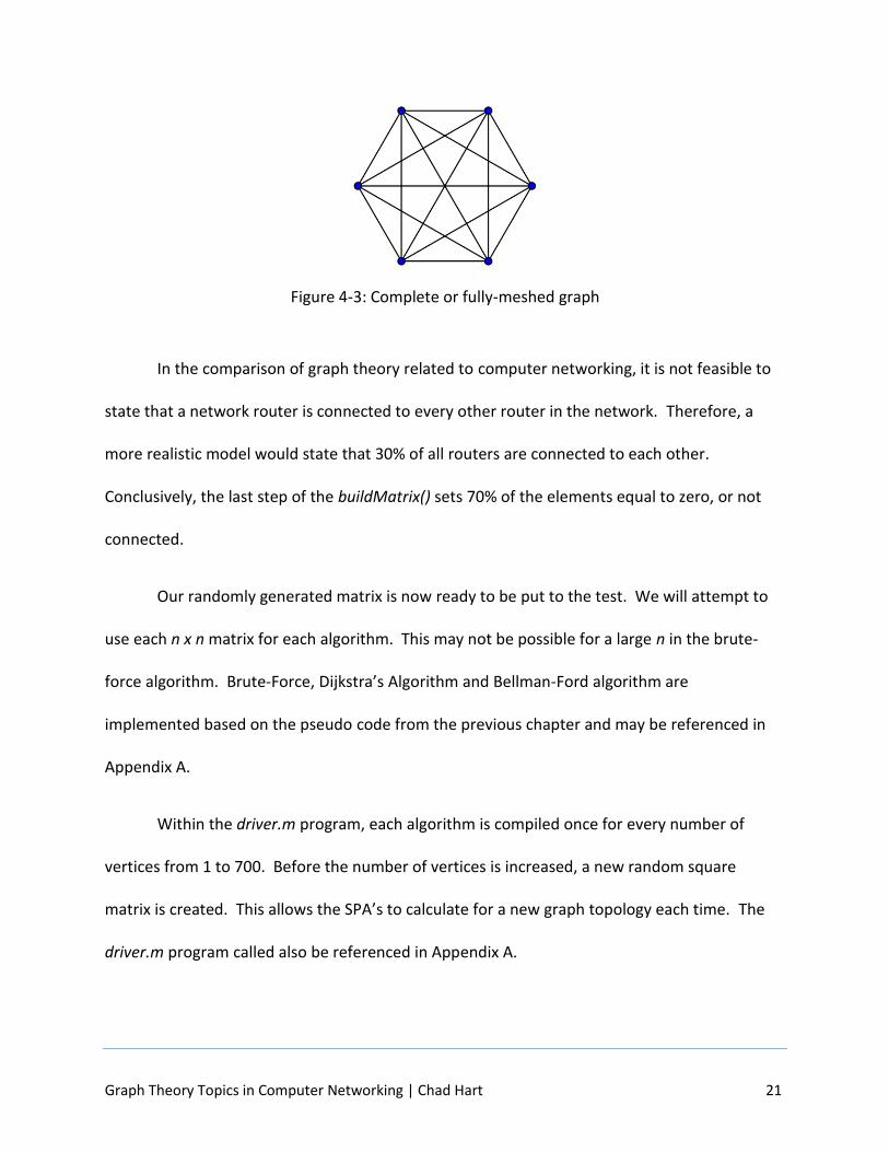
It was not practical to have each element in the graph, excluding the diagonal, set to a

value greater than zero. If each value was greater than zero, this would imply that the graph is

complete, or fully meshed. “A complete graph is a simple undirected graph in which every pair

of distinct vertices is connected by a unique edge. Figure 4-3 is an example of a complete graph

with six vertices.


Figure 4-3: Complete or fully-meshed graph

In the comparison of graph theory related to computer networking, it is not feasible to

state that a network router is connected to every other router in the network. Therefore, a

more realistic model would state that 30% of all routers are connected to each other.

Conclusively, the last step of the buildMatrix() sets 70% of the elements equal to zero, or not

connected.

Our randomly generated matrix is now ready to be put to the test. We will attempt to

use each n x n matrix for each algorithm. This may not be possible for a large n in the brute-

force algorithm. Brute-Force, Dijkstra’s Algorithm and Bellman-Ford algorithm are

implemented based on the pseudo code from the previous chapter and may be referenced in

Appendix A.

Within the driver.m program, each algorithm is compiled once for every number of

vertices from 1 to 700. Before the number of vertices is increased, a new random square

matrix is created. This allows the SPA’s to calculate for a new graph topology each time. The

driver.m program called also be referenced in Appendix A.


The “tic-toc” pre-defined MATLAB function is used each time to determine the time

taken for each algorithm to run. The time recordings are stored in to a variable called Results.

After the driver.m program has completed, we imported these values into a Microsoft Excel

spreadsheet in order to easily create graphs and mine the data easily.

Figure 4-4: Runtime results for Dijkstra vs. Bellman-Ford (1 to 450 vertices)

0

0.1

0.2

0.3

0.4

0.5

0.6

0.7

0.8

0.9

1

2

15

28

41

54

67

80

93

10

6

11

9

13

2

14

5

15

8

17

1

18

4

19

7

21

0

22

3

23

6

24

9

26

2

27

5

28

8

30

1

31

4

32

7

34

0

35

3

36

6

37

9

39

2

40

5

41

8

43

1

44

4

Tim

e in

Se

con

ds

Number of Vertices

Shortest Path Algorithm Runtime (450 Max)

Dijkstra Bellman-Ford


Figure 4-5: Runtime results for Dijkstra vs. Bellman-Ford (1 to 700 vertices)

Figure 4-4 & Figure 4-5 are line graphs from runtimes of both major SPA’s. Figure 4-4

exhibits 1 to 450 vertices while Figure 4-5 shows runtimes for 1 to 700 vertices. After running

the two single-source shortest path algorithms, it can be seen that the Bellman-Ford algorithm

is more efficient than Dijkstra’s algorithm up until the number of vertices in the graph reach

around 425. From this point, Dijkstra’s algorithm shows to be much more efficient as the

number of vertices approach infinity.

0

0.5

1

1.5

2

2.5

3

3.5

42

21

40

59

78

97

11

61

35

15

41

73

19

22

11

23

02

49

26

82

87

30

63

25

34

43

63

38

24

01

42

04

39

45

84

77

49

65

15

53

45

53

57

25

91

61

06

29

64

86

67

68

6

Tim

e in

Se

con

ds

Number of Vertices

Shortest Path Algorithm Runtime (700 Max)

Dijkstra Bellman-Ford


Chapter 5 – Conclusion

From the information provided in our Experimental data, it is obvious to see that the

brute-force algorithm is not efficient. However, this was expected because every possible path

was found without taking the cost into consideration. For very small networks, the brute-force

algorithm might be a valid method. It is certainly the easiest for elementary graph theorist to

comprehend, but it is not realistic to use this algorithm for very large numbers of vertices.

The Bellman-Ford algorithm and Dijkstra’s algorithm proved to be much more efficient

than brute-force, with Dijkstra proving to run in the least amount of time for very large

networks. It appears that for complete, fully meshed networks, the Bellman-Ford algorithm

actually ran faster than Dijkstra’s algorithm for networks of size 425 or less. However, Dijkstra

showed to be considerably more efficient beyond networks with more than 425 vertices.

In relation to computer networking, this will likely come as a shock to many network

engineers. As a general rule, network engineers are told to stay away from the routing

protocols that use the Bellman-Ford algorithm. Again, these protocols are RIP and EIGRP, while

OSPF runs Dijkstra’s algorithm. However, our studies show that for small and medium sized

networks, EIGRP and OSPF calculate the shortest path in a relatively close amount of time.

Therefore, it can be said that OSPF only needs to be chosen in very large networks. Otherwise,

in most cases, EIGRP and OSPF are very similar in their efficiencies.


Computer networking first sparked my interest fifteen years ago. Since graduating high

school, I was always intrigued with pursuing a career in Information Technology, so I soon

obtained a job as a network administrator. From that point, I decided to choose a specialization

within IT and focused on computer networking. From personal study and research, combined

with school courses, I found a position as a network engineer. I began working full time on

Cisco and HP networking products. I have been markedly thorough in understanding each and

every protocol within computer networking. In most cases within the industry, engineers make

their argument on which dynamic routing protocol is best based on factors that are not at all

related to mathematics. Often finding their arguments incomplete and frustrating, I set out to

analyze which protocol was based on an all-encompassing mathematical algorithm. I believe I

reached a successful analysis and look forward to more mathematical research endeavors in

the future.


References

1 Schrijver, Alexander. 2010. On the History of the Shortest Path Problem. Documenta

Math. p. 155-165.

2 Yellen, Jay and Gross, Jonathan. 2008. Graph Theory and its Applications. Chapman &

Hall. P. 172.

3 McHugh, James. Algorithmic Graph Theory. Prentice Hall. P. 92.

4 “Introduction to Algorithms – Lecture 18”. MIT 6.046J.

http://www.youtube.com/watch?v=Ttezuzs39nk

5 Wu, Bang Ye. Study of Shortest Path. Shortest-Path Trees.

6 R. Bellman. On a routing problem. Quar. Appl. Math., 16:87-90, 1958.

7 E.W. Dijkstra. A note on two problems in connection with graphs. Numer. Math.,

1:269–271, 1959.

http://www.youtube.com/watch?v=Ttezuzs39nk


Appendix A

Figure A-1: MATLAB code for Brute-Force Algorithm

% Author: Chad Hart

% Advisor: Dr. Tim Redl

% Title: Brute-Force Algorithm

% Description: This program implements the Brute-Force Shortest Path

Algorithm.

% The program will input a square matrix of any size n, which

% will denote the cost from one node to another. The rows of

% this matrix will define the cost "from" one node, while the

% columns will define the "to" cost.

%

% For example:

%

% [0 2 5]

% costs = [2 0 3]

% [5 3 0]

%

% The cost from node 2 to 3 is 3

%

% This program can be used for a directed or undirected graph.

% Please note that if the graph is undirected, the matrix

% should be symetric reflected accross the diagonal.

%

% The program will also input the source and destination node

function bruteForceDFS(costs, source, dest, path)

n = size(costs,1);

for i = 1:n

if costs(source,i) ~= 0 && sum(ismember(path,i)) == 0

if i == dest

[path i]

end

bruteForceDFS(costs,i,dest,[path i])

end

end

end


Figure A-2: MATLAB code for Dijkstra’s Algorithm

% Author: Chad Hart


% Title: Dijkstra's Algorithm

% Description: This program implements Dijkstra's Shortest Path Algorithm.





%

% For example:

%

% [0 2 5]

% costs = [2 0 3]

% [5 3 0]

%


%




%


function dijkstra(costs, source, dest)

n = size(costs, 1); % determine the size of S

S(1:n) = 0; % initialize S to all 0's

distance(1:n) = inf; % initialize distance vector to all inf

previous(1:n) = inf; % initialize previous node vector to all inf

distance(source) = 0; % set source distance to 0

while (sum(S) ~= n) % Run until all nodes are used

cand = []; % Choose possible candidates

for (i = 1:n)

if (S(i) == 0)

cand = [cand distance(i)];

else

cand = [cand inf];

end

end

[x u] = min(cand); % Choose the lowest candidate, x is not important

S(u) = 1; % Update S vector

for (i = 1:n) % Update distance vector if feasible

if (distance(u) + costs(u,i) < distance(i)) && (costs(u,i) ~= 0)

distance(i) = distance(u) + costs(u,i);

previous(i) = u;


end

end

end

distance % Output Distance vector

previous % Output Previous Node vector

ShortestPath = [dest];

traverse = dest;

while (previous(traverse) ~= source) % Traverse backwards to find path

ShortestPath = [previous(traverse) ShortestPath];

traverse = previous(traverse);

end

ShortestPath = [previous(traverse) ShortestPath]


Figure A-3: MATLAB code for Bellman-Ford Algorithm

% Author: Chad Hart


% Title: Bellman-Ford Algorithm

% Description: This program implements the Bellman-Ford Shortest Path

Algorithm.





%

% For example:

%

% [0 2 5]

% costs = [2 0 3]

% [5 3 0]

%


%




%


function bellmanford(costs, source, dest)

n = size(costs, 1); % determine the size of S

S(1:n) = 0; % initialize S to all 0's

distance(1:n) = inf; % initialize distance vector to all inf

previous(1:n) = inf; % initialize previous node vector to all inf

distance(source) = 0; % set source distance to 0

for (i = 1:n-1)

for (j = 1:n) % Update distance vector if feasible

for (k = 1:n)

if ((distance(j) + costs(j,k) < distance(k)) && (costs(j,k) ~=

0))

distance(k) = distance(j) + costs(j,k);

previous(k) = j;

end

end

end

end

% distance % Output Distance vector

% previous % Output Previous Node vector

ShortestPath = [dest];

traverse = dest;

while (previous(traverse) ~= source) % Traverse backwards to find path


ShortestPath = [previous(traverse) ShortestPath];

traverse = previous(traverse);

end

ShortestPath = [previous(traverse) ShortestPath]


Figure A-4: MATLAB code for driver.m

results=[];

for (i=1:3)

for (n=2:700)

randomMatrix = buildMatrix(n);

i

n

tic;

dijkstra(randomMatrix,1,2);

DijkstraTime = toc;

tic;

bellmanford(randomMatrix,1,2);

BellmanTime = toc;

results(n,3*i-2) = n;

results(n,3*i-1) = DijkstraTime;

results(n,3*i) = BellmanTime;

end

end

results

graph theory topics in computer networkingcms.uhd.edu/faculty/redlt/chadseniorproject.pdf · graph...

Documents