Graph Theory Fall 2019 – EPFL – Lecture Notes.

Lecturer: Friedrich Eisenbrand

November 29, 2019

Acknowledgements: These notes are heavily based on the lecture notes of the GraphTheory courses given by Istvan Tomon, Frank de Zeeuw, Andrey Kupavskii and DanielKorandi of the DCG group.

1

Lecture 1

Introduction

1 Definitions

Definition. A graph G = (V,E) consists of a finite set V and a set E of two-element subsetsof V . The elements of V are called vertices and the elements of E are called edges.

For instance, very formally we can introduce a graph like this:

V = 1, 2, 3, 4, E = 1, 2, 3, 4, 2, 3, 2, 4.In practice we more often think of a drawing like this:

1 2

34

Technically, this is what is called a labelled graph, but we often omit the labels. When wesay something about an unlabelled graph like , we mean that the statement holds for anylabelling of the vertices.

Here are two examples of related objects that we do not consider graphs in this course:

The first is a multigraph, which can have multiple edges and loops; the corresponding defini-tion would allow the edge set and the edges to be multisets. The second is a directed graph, inwhich every edge has a direction; in the corresponding definition the edges would be orderedpairs instead of two-element subsets.

Although this course is mostly not about these variants, in some cases it will be morenatural to state our results for directed or multigraphs. In any case, we will not treat infinitegraphs in this course.

Graphs (and their above-mentioned variants) are highly applicable in- and outside math-ematics because they provide a simple way of modeling many concepts involving connec-tions between objects. For example, graphs can model social networks (vertices=people &edges=friendships), computer networks (computers & links), molecules (atoms & bonds) andmany other things. The aim of this course is to study graphs in the abstract sense, and tointroduce the fundamental concepts, tools, tricks and results about them.

Some notation: Given a graph G, we write V (G) for the vertex set, and E(G) for theedge set. For an edge x, y ∈ E(G), we usually write xy, and we consider yx to be the sameedge. If xy ∈ E(G), then we say that x, y ∈ V (G) are adjacent or connected or that they areneighbors. If x ∈ e, then we say that x ∈ V (G) and e ∈ E(G) are incident.

Definition (Subgraphs). Two graphs G,G′ are isomorphic if there is a bijection ϕ : V (G)→V (G′) such that xy ∈ E(G) if and only if ϕ(x)ϕ(y) ∈ E(G′). A graph H is a subgraph of agraph G, denoted H ⊂ G, if there is a graph H ′ isomorphic to H such that V (H ′) ⊂ V (G)and E(H ′) ⊂ E(G).

2

With this definition we can for instance say that is a subgraph of . As mentionedabove, when we talk about graphs we often omit the labels of the vertices. A more formal wayof doing this is to define an unlabelled graph to be an isomorphism class of labelled graphs.We will be somewhat informal about this distinction, since it rarely leads to confusion.

Definition (Degree). Fix a graph G = (V,E). For v ∈ V , we write

N(v) = w ∈ V : vw ∈ E

for the set of neighbors of v (which does not include v). Then d(v) = |N(v)| is the degreeof v. We write δ(G) for the minimum degree of a vertex in G, and ∆(G) for the maximumdegree.

Definition (Examples). The following are some of the most common types of graphs.

• Paths are the graphs Pn of the form . The graph Pn has n− 1 edges and ndifferent vertices; we say that Pn has length n− 1.

• Cycles are the graphs Cn of the form . The graph Cn has n edges and ndifferent vertices; the length of Cn is defined to be n.

• Complete graphs (or cliques) are the graphs Kn on n vertices in which all vertices areadjacent. The graph Kn has

(n2

)edges. For instance, K4 is .

• The complete bipartite graphs are the graphs Ks,t with a partition V (Ks,t) = X ∪ Ywith |X| = s, |Y | = t, such that every vertex of X is adjacent to every vertex of Y , andthere are no edges inside X or Y . Then Kst has st edges. For example, K2,3 is .

The following are the most common properties of graphs that we will consider.

Definition (Bipartite). A graph G is bipartite if there is a partition V (G) = X ∪ Y suchthat every edge of G has one vertex in X and one in Y ; we call such a partition a bipartition.

Definition (Connected). A graph G is connected if for all x, y ∈ V (G) there is a path in Gfrom x to y (more formally, there is a path Pk which is a subgraph of G and whose endpointsare x and y).A connected component of G is a maximal connected subgraph of G (i.e., a connected subgraphthat is not contained in any larger connected subgraph). The connected components of G forma partition of V (G).

2 Basic Facts

In this section we prove some basic facts about graphs. It is a somewhat arbitrarycollection of statements, but we introduce them here to get used to the terminology and tosee some typical proof techniques.

Proposition 1.1. In any graph G we have∑

v∈V (G)

d(v) = 2|E(G)|.

Proof. We count the number of pairs (v, e) ∈ V (G)×E(G) such that v ∈ e, in two differentways. On the one hand, a vertex v is involved in d(v) such pairs, so the total number of suchpairs is

∑v∈V (G) d(v). On the other hand, every edge is involved in two such pairs, so the

number of pairs must equal 2|E(G)|.

3

What we used here is a very powerful proof technique in combinatorics, called doublecounting. The lemma itself is sometimes called the “handshake lemma” because it says thatat a party the number of shaken hands is twice the number of handshakes. It has usefulcorollaries, such as the fact that the number of odd-degree vertices in a graph must be even.

Next, we will describe a very important characterization of bipartite graphs. But first,we need two more definitions.

Definition (Walk). A walk is a sequence v1e1v2e2 . . . vk of (not necessarily distinct) verticesvi and edges ei such that ei = vivi+1. A closed walk is a walk with v1 = vk. The length ofthis walk is the number of edges, k − 1.

It is easy to see that paths are exactly walks with no repeating vertices, and cycles areexactly closed walks with no repeating vertices apart from v1 = vk.

Definition (Distance). The distance d(u, v) of two vertices u, v ∈ V (G) is the length of theshortest path (or walk) in G from u to v. (If there is no u-v path in G then d(u, v) =∞.)

Now we are ready to prove the characterization. Note that “contains a cycle” means thatthe graph has a subgraph that is isomorphic to some Cn, and similarly for paths. An “oddcycle” is just a cycle whose length is odd.

Theorem 1.2. A graph is bipartite if and only if it contains no odd cycle.

Proof. To prove the easy direction of the statement, suppose that G is bipartite with bipar-tition V (G) = X ∪ Y , and let v1 · · · vkv1 be a cycle in G with, say, v1 ∈ X. We must havevi ∈ X for all odd i and vi ∈ Y for all even i. Since vk is adjacent to v1, it must be in Y , sok must be even and the cycle is not odd.

Now for the other direction, suppose G has no odd cycles. We may assume that G isconnected. Indeed, otherwise we can apply the same argument to each connected componentGi of G to get a bipartition Xi ∪ Yi of Gi. Choosing X = ∪iXi and Y = ∪iYi will then givea bipartition of G.

So if v is a fixed vertex, then every other vertex u ∈ V (G) has finite distance from v. Let

X = u : distance of v and u is evenY = u : distance of v and u is odd.

Our aim is to prove that this is a bipartition of G. For this, we need to check that no twovertices in X are adjacent and no two vertices in Y are adjacent.

Suppose for contradiction that some two vertices u1, u2 ∈ X are adjacent, and let e bethe edge u1u2. By construction, there are paths P1 from v to u1 and P2 from u2 to v thatboth have even lengths. But then joining P1, P2 and the edge e gives a closed walk P1eP2

of odd length, so by Claim 1.3 below, G contains an odd cycle, as well, contradiction theassumption. (Note that P1eP2 is not necessarily a cycle because P1 and P2 might intersect!)

We can do the same to show that no two vertices u1, u2 ∈ Y are adjacent: here the pathsP1, P2 will both have odd lengths, so again P1eP2 is a closed odd walk. So X ∪ Y is indeeda bipartition of G.

The proof above is a constructive argument, where we explicitly constructed the objectwe were looking for (and then proved that it satisfies the required properties). Of course, westill need to prove the following lemma to complete the proof. We use an inductive argument.

Claim 1.3. Every closed walk of odd length contains an odd cycle.

4

Proof. We apply induction on the length k of the walk. Since there is no closed walk oflength 1, the statement is vacuously true for k = 1. We could use this as the base case, butit is also easy to see that the only closed walk of length 3 is the triangle (K3), which itself isan odd cycle.

Now suppose the statement is true for every odd length < k, and let W = v1e1v2 . . . vk+1

be a closed walk of odd length k. Let j be the smallest index such that vi = vj for somei < j. We have two cases. If j − i is even, then deleting the j − i edges ei, . . . , ej−1 from Wyields another closed walk W ′ ⊆ W of odd length. Applying induction on W ′ then gives anodd cycle in W ′ and hence in W .

On the other hand, if j − i is odd (and it cannot be 1, so j − i ≥ 3), then the j − i edgesei, . . . , ej−1 form an odd cycle. Indeed, they form an odd walk without repeated vertices bythe choice of vj. This is what we were looking for.

3 Second Lecture: Teaser

The next theorem shows that if a graph has many edges, then it must contain a longpath.

Theorem 1.4. Let k ≥ 2 be an integer and let G be a graph on n vertices with at least(k − 1)n edges. Then G contains a path of length k.

The proof of this theorem is the combination of two lemmas, which are interesting ontheir own.

First, we consider the special case when every degree of G is large.

Lemma 1.5. If the minimum degree of G is k, then G contains a path of length k.

Proof. Let v1 · · · vl be a maximal path in G, i.e., a path that cannot be extended. Then anyneighbor of v1 must be on the path, since otherwise we could extend it. Since v1 has at leastk neighbors, the set v2, . . . , vl must contain at least k elements. Hence l ≥ k + 1, so thepath has length at least k.

Note that in general this bound cannot be improved, because the complete graph Kk+1

has minimum degree k, but its longest path has length k. In problem set 1, we will prove ananalogous statement for cycles.

5

Lecture 2

Basic results. Trees.

1 More basic facts

The next theorem shows that if a graph has many edges, then it must contain a longpath.

Theorem 2.6. Let k ≥ 2 be an integer and let G be a graph on n vertices with at least(k − 1)n edges. Then G contains a path of length k.

Proof. The proof of this theorem is the combination of two lemmas, which are interesting ontheir own.

First, we consider the special case when every degree of G is large.

Lemma 2.7. If the minimum degree of G is k, then G contains a path of length k.

Proof. Let v1 · · · vl be a maximal path in G, i.e., a path that cannot be extended. Then anyneighbor of v1 must be on the path, since otherwise we could extend it. Since v1 has at leastk neighbors, the set v2, . . . , vl must contain at least k elements. Hence l ≥ k + 1, so thepath has length at least k.

Note that in general this bound cannot be improved, because the complete graph Kk+1

has minimum degree k, but its longest path has length k. In problem set 1, we will prove ananalogous statement for cycles.

The next statement shows that every graph with sufficiently many edges must contain asubgraph with large minimum degree. We give an inductive proof, although it could also beproved using an algorithmic argument.

Lemma 2.8. Let G be graph on n vertices with at least (k − 1)n edges. Then G contains asubgraph H with δ(H) ≥ k.

Proof. We proceed by induction on n. Note that n ≤ 2(k − 1) is impossible because such agraph has at most n(n − 1)/2 < n(k − 1) edges. Also, for n = 2k − 1 the only graph withn(k − 1) edges is Kn = K2k−1, which has minimum degree 2k − 2, so we can take H = G.

Now suppose n > 2k − 1. If δ(G) ≥ k, then we can take H = G. Otherwise, thereis a vertex v of degree d(v) ≤ k − 1. Let G′ = G − v be the subgraph we obtain fromG by deleting v and all the edges touching it. Then G′ has n − 1 vertices and at leastn(k − 1)− (k − 1) = (n− 1)(k − 1) edges, so by induction, there is a subgraph H ⊆ G′ ⊆ Gsuch that δ(H) ≥ k.

We are done, as G contains a subgraph H with minimum degree at least k by Lemma2.8, and H contains a path of length k by Lemma 2.7. But then G contains a path of lengthk as well.

The following lemma can be helpful when trying to prove certain statements for generalgraphs that are easier to prove for bipartite graphs. The lemma says that you don’t have toremove more than half the edges of a graph to make it bipartite. The proof is an example ofan algorithmic proof, where we prove the existence of an object by giving an algorithm thatconstructs such an object.

6

Proposition 2.9. Any graph G contains a bipartite subgraph H with |E(H)| ≥ |E(G)|/2.

Proof. We prove the stronger claim that G has a bipartite subgraph H with V (H) = V (G)and dH(v) ≥ dG(v)/2 for all v ∈ V (G). Starting with an arbitrary partition V (G) = X ∪ Y(which need not be a bipartition for G), we apply the following procedure. We refer to Xand Y as “parts”. For any v ∈ V (G), we see if it has more edges to X or to Y ; if it has moreedges that connect it to the part it is in than it has edges to the other part, then we move itto the other part. We repeat this until there are no more vertices v that should be moved.

There are at most |V (G)| consecutive steps in which no vertex is moved, since if none ofthe vertices can be moved, then we are done. When we move a vertex from one part to theother, we increase the number of edges between X and Y (note that a vertex may move backand forth between X and Y , but still the total number of edges between X and Y increasesin every step). It follows that this procedure terminates, since there are only finitely manyedges in the graph. When it has terminated, every vertex in X has at least half its edgesgoing to Y , and similarly every vertex in Y has at least half its edges going to X. Thus thegraph H with V (H) = V (G) and E(H) = xy ∈ E(G) : x ∈ X, y ∈ Y has the claimedproperty that dH(v) ≥ dG(v)/2 for all v ∈ V (G).

The following is an easy but important fact. Its proof is extremal.

Proposition 2.10. Every u-v walk W contains a u-v path.

Proof. Let v1v2 . . . vk be a shortest u-v walk in W (more precisely, in the graph defined bythe edges of W ), so u = v1 and v = vk. We claim that this walk is in fact a path. Indeed,if vi = vj for some i < j, then v1v2 . . . vivj+1 . . . vk is also a u-v walk, and it is shorter (hasfewer edges), which is not possible. So the shortest walk has no repeated vertices, i.e., it isa path.

This fact has the useful corollaries that we can replace paths with walks in some of ourdefinitions:

• The distance d(u, v) is equal to the length of the shortest u-v walk.

• A graph is connected if and only if every pair of vertices u, v is connected by a walk.

The latter connectivity property is sometimes easier to check. Also, it clearly implies thatconnectivity is an equivalence relation.

Our last basic result gives a connection between the number of edges and the number ofconnected components in a graph.

Proposition 2.11. If a graph G has n vertices and k edges, then it has at least n − kcomponents.

Proof. Let us start with the empty graph and add the edges of G to it one-by-one. At thebeginning there are n vertices and no edges, so we have n components. Each added edgetouches at most 2 of the components, and joins these components if they are different (anedge within a component does not affect any components). This means that adding an edgedecreases the number of components by at most 1. Adding k edges therefore decreases thenumber of components by at most k, so after adding all k edges of G, we are left with atleast n− k of them.

Corollary 2.12. Every connected graph on n vertices has at least n− 1 edges.

7

2 Trees

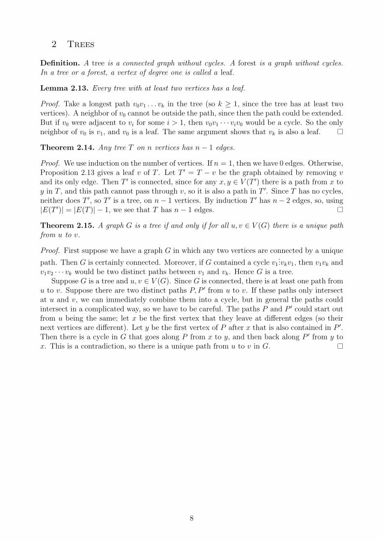
Definition. A tree is a connected graph without cycles. A forest is a graph without cycles.In a tree or a forest, a vertex of degree one is called a leaf.

Lemma 2.13. Every tree with at least two vertices has a leaf.

Proof. Take a longest path v0v1 . . . vk in the tree (so k ≥ 1, since the tree has at least twovertices). A neighbor of v0 cannot be outside the path, since then the path could be extended.But if v0 were adjacent to vi for some i > 1, then v0v1 · · · viv0 would be a cycle. So the onlyneighbor of v0 is v1, and v0 is a leaf. The same argument shows that vk is also a leaf.

Theorem 2.14. Any tree T on n vertices has n− 1 edges.

Proof. We use induction on the number of vertices. If n = 1, then we have 0 edges. Otherwise,Proposition 2.13 gives a leaf v of T . Let T ′ = T − v be the graph obtained by removing vand its only edge. Then T ′ is connected, since for any x, y ∈ V (T ′) there is a path from x toy in T , and this path cannot pass through v, so it is also a path in T ′. Since T has no cycles,neither does T ′, so T ′ is a tree, on n− 1 vertices. By induction T ′ has n− 2 edges, so, using|E(T ′)| = |E(T )| − 1, we see that T has n− 1 edges.

Theorem 2.15. A graph G is a tree if and only if for all u, v ∈ V (G) there is a unique pathfrom u to v.

Proof. First suppose we have a graph G in which any two vertices are connected by a unique

path. Then G is certainly connected. Moreover, if G contained a cycle v1...vkv1, then v1vk and

v1v2 · · · vk would be two distinct paths between v1 and vk. Hence G is a tree.Suppose G is a tree and u, v ∈ V (G). Since G is connected, there is at least one path from

u to v. Suppose there are two distinct paths P, P ′ from u to v. If these paths only intersectat u and v, we can immediately combine them into a cycle, but in general the paths couldintersect in a complicated way, so we have to be careful. The paths P and P ′ could start outfrom u being the same; let x be the first vertex that they leave at different edges (so theirnext vertices are different). Let y be the first vertex of P after x that is also contained in P ′.Then there is a cycle in G that goes along P from x to y, and then back along P ′ from y tox. This is a contradiction, so there is a unique path from u to v in G.

8

Lecture 3

BFS. Euler tours.

1 Breadth-first search

Definition. A spanning tree of a graph G is a subgraph T ⊆ G, which is a tree with V (T ) =V (G).

Our aim is to show that

Theorem 3.16. Every connected graph has a spanning tree.

We start with the greedy algorithm. For this, we assume that the edges are indexed bye1, . . . , em.

Algorithm 1. Unweighted Greedy

Initialize the edge set F = ∅for i = 1, . . . ,m

if (V, F + ei) does not contain a cycleF = F + ei

Theorem 3.17. Let F be constructed by the procedure in Algorithm 2. If G is connected,then (V, F ) is a spanning tree.

Proof. Clearly, (V, F ) has no cycles. We only have to show that (V, F ) is connected. Letx = v1, . . . , vl = y be a path connecting x and in y in G. And suppose that x and y arenot connected in (V, F ), then let k ≥ 2 be minimal such that v1 and vk are not connectedin (V, F ). The edge vk−1vk has not been inserted by the greedy algorithm. This means thatthere is a path from vk−1 to vk in (V, F ). This means that vk can be reached from v1 in(V, F ), a contradiction.

In the minimum weight spanning tree problem we are given a connected graph and aweight function w : E → R. The goal is to find a spanning tree T = (V, F ) such thatw(F ) ≤ w(F ′) for each spanning tree (V, F ′) of G. This is computed by the weighted greedyalgorithm.

Algorithm 2. Weighted Greedy

Sort the edges in increasing order according to weight:w(e1) ≤ w(e2) ≤ · · · ≤ w(em)Initialize the edge set F = ∅for i = 1, . . . ,m

if (V, F + ei) does not contain a cycleF = F + ei

Theorem 3.18. The weighted greedy algorithm finds a minimum weight spanning tree.

9

Proof. Theorem 3.18 shows that T is a tree. Let |V | = n and suppose that the edges of Tare eπ1 , . . . , eπn−1 and that they are picked in that order. Let TOPT be a minimum weightspanning tree for which the smallest k such that eπk is not an edge of TOPT is maximal.

Inserting eπk into TOPT results in a cycle that does not only contain edges of T . Let e bean edge on this cycle that does not belong to T . This edge must be after ek in the orderingof the edges according to their weight, since the edges eπ1 , . . . , eπk−1

also belong to TOPT andsince any other edge before eπk creates a cycle in eπ1 , . . . , eπk−1

.This means that w(e) ≤ w(eπk). Thus TOPT + eπk − e is an optimal spanning tree which

contradicts the maximality of k.

We next describe a spanning tree that is called breadth-first-search tree. To this end,let s ∈ V be a starting vertex and let Vi = v ∈ V : d(s, v) = i be the vertices that havedistance i from s. Let k be the largest distance of a vertex from s that is connected to s. Wecan build a tree as follows.

Initialize the edge set F = ∅.for i = 1, . . . , k

for each v ∈ Vi :choose u ∈ Vi−1 with uv ∈ E.F = F + uv

Let V ′ = ∪ki=0Vi. The graph TBFS = (V ′, F ) is connected, since one can reach s from anyvertex by following their edge “downwards”. Also |F | = |V ′| − 1 which implies that TBFS isa tree. It is a breadth-first-search tree. The unique path from s to any other vertex in TBFSis a shortest path from s to that vertex in G. It is computed by the following algorithm.

Algorithm 3 (Breadth-First-Search).

Initialize: F = ∅, queue Q = sLabel each vertex v ∈ V \ s unknownLabel s knownwhile Q is not empty

u = head(Q)dequeue(u)for each v ∈ N(u)

if v is unknownlabel v as knownF = F + uvenqueue v

The algorithm computes a bfs-tree in a bottom up manner. The following are claims thatare easily verified by induction.

Lemma 3.19. For each i = 0, . . . , k, there is a moment in time, when Q contains exactlyVi, all vertices in ∪ij=0Vj are labeled as known and all other vertices are labeled as unknown.Furthermore (∪ij=0Vj, F ) is a tree in which the unique path from s to any other vertex is ashortest path in G.

Definition. The diameter of a graph G is the largest distance among any pairs of vertices:diam(G) = maxx,y∈V (G) d(x, y). If G is disconnected, then diam(G) =∞.

10

BFS has a number of applications in providing fairly (or very) efficient algorithms forsolving certain tasks on graphs. For example:

• Find a shortest path from xu to v in G: Run the algorithm with root u to get a treeT . The unique path from u to v in T (which exists by Lemma 2.15) is a shortest path.

• Find the connected components of G: Run the algorithm with some root r. The verticesexplored by BFS are exactly the component of r. If there is an unexplored vertex r′,run BFS again from r′ as a root. Repeat until all vertices are visited. This actuallygives a spanning forest of G.

• Compute diam(G): For each pair of vertices, we can find a shortest path and thus thedistance. Do this for all pairs and take the largest distance.

• Find a shortest cycle in G: For every edge uv, find a shortest path between u and vin G− uv (if it exists), then combine this path with uv to get a cycle. (This will be ashortest cycle through uv.) Compare all these cycles to find the shortest.

• Determine if G is bipartite: Determine the connected components of G. In everycomponent H, select a root r, and partition the vertices into X = x ∈ V (H) :d(r, x) is even and Y = y ∈ V (H) : d(r, y) is odd. Then H is bipartite if and onlyif X and Y have no internal edges (see the proof of Theorem 1.2), and G is bipartite ifand only if every component is bipartite.

Not all of these algorithms are the most efficient, but they are already much better thanbrute force approaches that go over all possible answers. There are all kinds of algorithmsthat do these tasks faster, but in this course, we don’t care too much about efficiency, andwe focus on the graph-theoretical aspects (in particular, proving that the algorithms work).

We should emphasize, though, that for finding shortest paths between two vertices, BFSis the best general algorithm. For example, Dijkstra’s algorithm, a variant of BFS that worksfor graphs with positive edge weights (representing, e.g, the lengths of streets) is directlyused by routing softwares.

2 Euler tours

Definition. A trail is a walk with no repeated edges. A tour is a closed trail (i.e., one thatstarts and ends at the same vertex).

Definition. An Euler (or Eulerian) trail in a (multi)graph G = (V,E) is a trail in G passingthrough every edge (exactly once). An Euler tour is a tour in G passing through every edge.

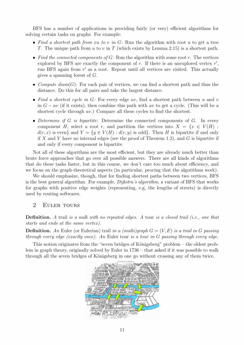
This notion originates from the “seven bridges of Konigsberg” problem – the oldest prob-lem in graph theory, originally solved by Euler in 1736 – that asked if it was possible to walkthrough all the seven bridges of Konigsberg in one go without crossing any of them twice.

11

This question can be turned into a graph problem asking for an Euler trail. Euler solvedthe problem by noticing that the existence of Euler trails is closely related to the degreeparities.

Theorem 3.20. A connected (multi)graph has an Eulerian tour if and only if each vertexhas even degree.

The proof of this theorem is based on the following simple lemma.

Lemma 3.21. In a graph where all vertices have even degree, every maximal trail is a closedtrail.

Proof. Let T be a maximal trail. If T is not closed, then T has an odd number of edgesincident to the final vertex v. However, as v has even degree, there is an edge touching vthat is not contained in T . This edge can be used to extend T to a longer trail, contradictingthe maximality of T .

Proof of Theorem 3.20. To see that the condition is necessary, suppose G has an Euleriantour C. If a vertex v was visited k times in the tour C, then each visit used 2 edges incidentto v (one incoming edge and one outgoing edge). Thus, d(v) = 2k, which is even.

To see that the condition is sufficient, let G be a connected graph with even degrees. LetT = e1e2 . . . e` (where ei = (vi−1, vi)) be a longest trail in G. Then it is maximal, of course.According to the Lemma, T is closed, i.e., v0 = v`. G is connected, so if T does not includeall the edges of G then there is an edge e outside of T that touches it, i.e., e = uvi for somevertex vi in T . Since T is closed, we can start walking through it at any vertex. But if westart at vi then we can append the edge e at the end: T ′ = ei+1 . . . e`e1e2 . . . eie is a trail inG which is longer than T , contradicting the fact that T is a longest trail in G. Thus, T mustinclude all the edges of G and so it is an Eulerian tour.

Corollary 3.22. A connected multigraph G has an Euler trail if and only if it has either 0or 2 vertices of odd degree.

Proof. Suppose T is an Euler trail from vertex u to vertex v. If u = v then T is an Euleriantour and so by Theorem 3.20, it follows that all the vertices in G have even degree. If u 6= vthen let us add a new edge e = uv to G. In this new multigraph G∪e, T ∪e is an Eulertour. By Theorem 3.20 we see that all the degrees in G ∪ e are even. This means that inthe original multigraph G, the vertices u, v are the only ones that have odd degree.

Now we prove the other direction of the corollary. If G has no vertices of odd degree thenby Theorem 3.20 it contains an Eulerian tour which is also an Eulerian trail. Suppose nowthat G has 2 vertices u, v of odd degree. Then add a new edge e to G. Now all vertices ofthe resulting multigraph G ∪ e have even degree, so, by Theorem 3.20, it has an Euleriantour C. Removing the edge e from C gives an Eulerian trail of G from u to v.

12

Lecture 4

Hamilton cycles.

Euler trails are walks that use each edge exactly once. But what if we want to use eachvertex exactly once?

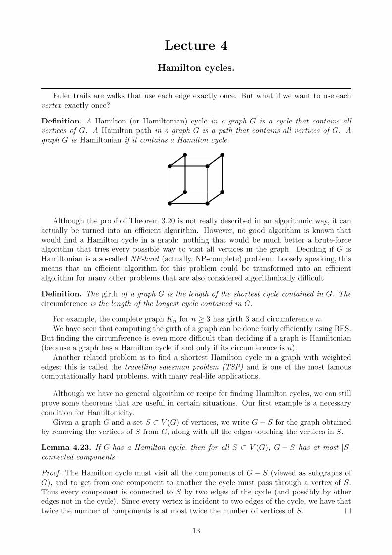
Definition. A Hamilton (or Hamiltonian) cycle in a graph G is a cycle that contains allvertices of G. A Hamilton path in a graph G is a path that contains all vertices of G. Agraph G is Hamiltonian if it contains a Hamilton cycle.

Although the proof of Theorem 3.20 is not really described in an algorithmic way, it canactually be turned into an efficient algorithm. However, no good algorithm is known thatwould find a Hamilton cycle in a graph: nothing that would be much better a brute-forcealgorithm that tries every possible way to visit all vertices in the graph. Deciding if G isHamiltonian is a so-called NP-hard (actually, NP-complete) problem. Loosely speaking, thismeans that an efficient algorithm for this problem could be transformed into an efficientalgorithm for many other problems that are also considered algorithmically difficult.

Definition. The girth of a graph G is the length of the shortest cycle contained in G. Thecircumference is the length of the longest cycle contained in G.

For example, the complete graph Kn for n ≥ 3 has girth 3 and circumference n.We have seen that computing the girth of a graph can be done fairly efficiently using BFS.

But finding the circumference is even more difficult than deciding if a graph is Hamiltonian(because a graph has a Hamilton cycle if and only if its circumference is n).

Another related problem is to find a shortest Hamilton cycle in a graph with weightededges; this is called the travelling salesman problem (TSP) and is one of the most famouscomputationally hard problems, with many real-life applications.

Although we have no general algorithm or recipe for finding Hamilton cycles, we can stillprove some theorems that are useful in certain situations. Our first example is a necessarycondition for Hamiltonicity.

Given a graph G and a set S ⊂ V (G) of vertices, we write G− S for the graph obtainedby removing the vertices of S from G, along with all the edges touching the vertices in S.

Lemma 4.23. If G has a Hamilton cycle, then for all S ⊂ V (G), G − S has at most |S|connected components.

Proof. The Hamilton cycle must visit all the components of G− S (viewed as subgraphs ofG), and to get from one component to another the cycle must pass through a vertex of S.Thus every component is connected to S by two edges of the cycle (and possibly by otheredges not in the cycle). Since every vertex is incident to two edges of the cycle, we have thattwice the number of components is at most twice the number of vertices of S.

13

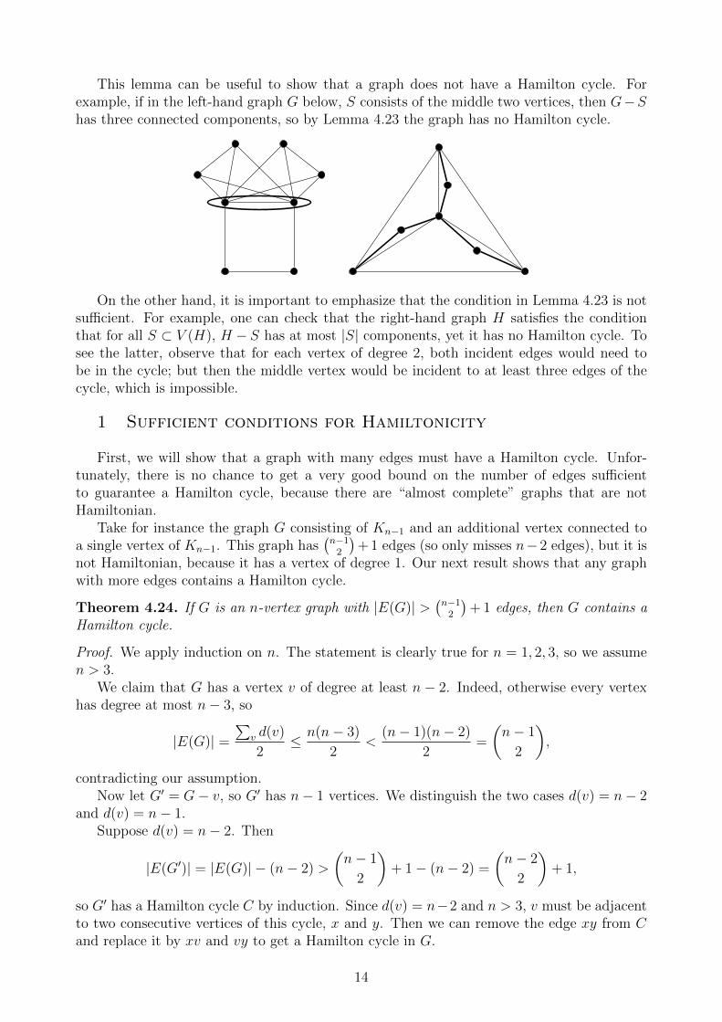
This lemma can be useful to show that a graph does not have a Hamilton cycle. Forexample, if in the left-hand graph G below, S consists of the middle two vertices, then G−Shas three connected components, so by Lemma 4.23 the graph has no Hamilton cycle.

On the other hand, it is important to emphasize that the condition in Lemma 4.23 is notsufficient. For example, one can check that the right-hand graph H satisfies the conditionthat for all S ⊂ V (H), H − S has at most |S| components, yet it has no Hamilton cycle. Tosee the latter, observe that for each vertex of degree 2, both incident edges would need tobe in the cycle; but then the middle vertex would be incident to at least three edges of thecycle, which is impossible.

1 Sufficient conditions for Hamiltonicity

First, we will show that a graph with many edges must have a Hamilton cycle. Unfor-tunately, there is no chance to get a very good bound on the number of edges sufficientto guarantee a Hamilton cycle, because there are “almost complete” graphs that are notHamiltonian.

Take for instance the graph G consisting of Kn−1 and an additional vertex connected toa single vertex of Kn−1. This graph has

(n−1

2

)+ 1 edges (so only misses n− 2 edges), but it is

not Hamiltonian, because it has a vertex of degree 1. Our next result shows that any graphwith more edges contains a Hamilton cycle.

Theorem 4.24. If G is an n-vertex graph with |E(G)| >(n−1

2

)+ 1 edges, then G contains a

Hamilton cycle.

Proof. We apply induction on n. The statement is clearly true for n = 1, 2, 3, so we assumen > 3.

We claim that G has a vertex v of degree at least n − 2. Indeed, otherwise every vertexhas degree at most n− 3, so

|E(G)| =∑

v d(v)

2≤ n(n− 3)

2<

(n− 1)(n− 2)

2=

(n− 1

2

),

contradicting our assumption.Now let G′ = G− v, so G′ has n− 1 vertices. We distinguish the two cases d(v) = n− 2

and d(v) = n− 1.Suppose d(v) = n− 2. Then

|E(G′)| = |E(G)| − (n− 2) >

(n− 1

2

)+ 1− (n− 2) =

(n− 2

2

)+ 1,

so G′ has a Hamilton cycle C by induction. Since d(v) = n−2 and n > 3, v must be adjacentto two consecutive vertices of this cycle, x and y. Then we can remove the edge xy from Cand replace it by xv and vy to get a Hamilton cycle in G.

14

Now suppose d(v) = n−1. In this case we only have |E(G′)| >(n−2

2

), so we cannot apply

induction right away. If G′ is complete, then G′ has a Hamilton cycle, and we can add v asin the previous case (in fact, as d(v) = n− 1, v is now adjacent to every vertex of the cycle).

Otherwise, there is an edge xy missing from G′. Let us look at the graph G′ + xy thatwe get by adding xy to G′. Now this graph has more than

(n−2

2

)+ 1 edges, so we can apply

induction to find a Hamilton cycle C in it. If C does not contain xy, then we can again addv as in the previous case. If C does contain xy, then replacing xy with the path xvy in Cgives a Hamilton cycle in G.

As mentioned before, the condition in the theorem above is somewhat weak in the sensethat many graphs that have a Hamilton cycle do not satisfy the condition. The followingsufficient condition does better by looking at the minimum degree instead of the total numberof edges. Note that we have previously seen that every graph G has a cycle of length at leastδ(G)+1. The following theorem says that something much stronger is true when the minimumdegree is at least |V (G)|/2.

Theorem 4.25 (Dirac). Let G be a graph on n ≥ 3 vertices. If δ(G) ≥ n2, then G contains

a Hamilton cycle.

Proof. First observe that G must be connected, because each component contains at leastδ(G) + 1 > n/2 vertices, so G cannot have more than one components.

Take a longest path P = v1v2 . . . vk in G. By maximality, all neighbors of v1 and vk arein the path. Let us say that an edge vivi+1 is type-1 if vi+1 ∈ N(v1), and let us say that itis type-2 if vi ∈ N(vk). As δ(G) ≥ n/2, we have at least n/2 type-1 and n/2 type-2 edgesin P . But P has at most n − 1 edges, so some edge vjvj+1 is both type-1 and type-2, i.e.,v1vj+1 and vjvk are edges of G. Then C = P − vjvj+1 + v1vj+1 + vjvk = vj . . . v1vj+1 . . . vkviis a cycle.

In fact, C is a Hamilton cycle. Indeed, suppose not all vertices are contained in C. SinceG is connected, there must be an edge uvi where u /∈ C. Then there is a path that goes fromu to vi and then all around the cycle C to a neighbor of vi. This path contains k+ 1 vertices,contradicting the maximality of P .

This theorem is again best possible, in the sense that a weaker bound on the minimumdegree would not imply a Hamilton cycle. Take for instance the graph G consisting of twocopies of Kk sharing a single vertex. This graph has n = 2k−1 vertices and minimum degreeδ(G) = k − 1 = n−1

2, but no Hamilton cycle, because deleting the shared vertex creates two

components, contradicting Lemma 4.23.It is easy to check that the proof of Dirac’s theorem works for the following strengthening,

as well:

Theorem 4.26 (Ore). Let G be a graph on n ≥ 3 vertices. If d(u) + d(v) ≥ n for anynon-adjacent vertices u and v, then G contains a Hamilton cycle.

Using this theorem, one can also obtain a short proof of Theorem 4.24 (see problem set),so one can think of Ore’s theorem as a common generalization of Theorems 4.24 and 4.25.

Definition. A tournament is a directed graph that has exactly one (oriented) edge betweenany two vertices.

For example, if we take a complete graph and give each edge an orientation then we geta tournament. We use u→ v to denote that there is an edge uv directed from u to v. Whatis the longest directed path in such a graph?

15

Theorem 4.27. Every tournament contains a directed Hamilton path.

Proof. We do induction on the number of vertices n. For n = 2, there is nothing to prove,since one can take the only edge of the tournament as the Hamilton path. Now supposen > 2, and let v be a vertex of T . By induction, T − v has a Hamilton path P = v1v2 . . . vn.If v → v1 or vn → v, then vv1v2 . . . vn or v1v2 . . . vnv is a Hamilton path in T . So assumev1 → v and v → vn. But then there must be a vertex vi with 1 ≤ i ≤ n− 1, such that vi → vand v → vi+1, so v1v2 . . . vivvi+1vi+2 . . . vn is a Hamilton path in T .

Of course, not every tournament contains a directed Hamilton cycle. In fact, there is atournament that does not contain any cycle, whatsoever: the so-called transitive tournamenton vertex set 1, . . . , n where each edge is oriented from the smaller endpoint to the largerone.

16

Lecture 5

Matchings.

Recall that a matching M is a set of vertex-disjoint edges. A perfect matching M ina graph G is a matching that touches every vertex of G. In other words, it is a 1-regularsubgraph of G (recall that a graph is k-regular if all degrees equal k).

1 Stable matchings

Suppose that you have n students that want to do their internships in n companies. Eachhave sent their applications to all the companies. Each student and each company has theirlist of preferences, and we want to pair up the students with the companies so that thisassignment is stable in the following sense: there is no student and company that would bothprefer to work with each other rather than their assigned pairs.

More formally, consider a bipartite graph G with parts A, B, where |A| = |B| = n, andin which each vertex has a (strict) order of preferences for the vertices of the other part. Wesay that a perfect matching is stable, if there is no pair a ∈ A, b ∈ B, such that both of themwould prefer the other to the vertex they are currently matched to.

Below we present an algorithm of Gale and Shapley, which allows to construct such astable matching.

The Gale-Shapley Algorithm to find a stable matching M in a complete bipartitegraph G = (A ∪B,E) with |A| = |B|

(1) Set M = ∅;

(2) Iterate:

(a) Take an unmatched vertex a ∈ A and let b ∈ B be the vertex that a prefersamong the ones a has not tried yet.

(b) a “proposes” to b: If b is unmatched or b is matched to a′, but prefers a over a′,then “accept” a and “reject” a′: put M := M − a′b+ ab. Otherwise, “reject”:leave M unchanged;

(c) If there is no more unmatched vertices in A that have someone left on the list,then go to (3);

(3) Return M .

Proposition 5.28. The matching M that the algorithm outputs is stable.

Proof. First we show that M is perfect. Indeed, if there is a pair of vertices a ∈ A, b ∈ B,such that both are not in the matching, then a must have proposed to b at some point.However, if a vertex b ∈ B is in M at some step of the algorithm, then it stays in M .

Next, we show that the matching is stable. Assume that ab /∈M. Upon completion of thealgorithm, it is not possible for both a and b to prefer each other over their current match.If a prefers b to its match, then a must have proposed to b before its current match. If baccepted its proposal, but is matched to another vertex at the end, then b prefers the currentmatch of b over a. If b rejected the proposal of a, then b was already matched to a vertexthat is better for b.

17

2 Maximum matchings

The previous problem was about perfect matchings in a complete bipartite graph. Butnot every graph has a perfect matching. So how can we find a largest or maximum matching?(Not to be confused with a maximal matching, which just means that it cannot be extended,i.e., no larger matching contains it as a subgraph.) How can we even tell if a graph has aperfect matching? How can we check if a given matching is maximum?

First, note that a maximal matching need not be maximum. Take for instance a path withthree edges, and the matching consisting of the middle edge. Similarly, a greedy approach thatkeeps adding edges without removing any, like we used for spanning trees, would probably notlead to a maximum matching. Instead, an algorithm to find maximum matchings will needsome kind of backtracking, where we throw away some edges that we previously selected.The following notion lets us do that in a smart way.

Definition. Given a matching M in a bipartite graph G, a path is alternating if among anytwo consecutive edges on the path, exactly one is in M . An alternating path with at least oneedge is augmenting if its first and last vertices are not covered by M .

Note that an augmenting path always has odd length.

Lemma 5.29. A matching M is maximum if and only if there is no augmenting path for M .

Proof. We prove that M is not maximum if and only if there is an augmenting path forM . First suppose that there is an augmenting path P = v1v2 . . . v2k for the matching M .So v2v3, . . . , v2iv2i+1, . . . , v2k−2v2k−1 ∈ M . Then we can get a larger matching by removingthese edges from M and replacing them by v1v2, . . . , v2i−1v2i, . . . , v2k−1v2k. In other words,we replace M by M ′ = M4E(P ).1 Then M ′ is a matching since v1 and vk were unmatchedby M , and we have |M ′| = |M |+ 1, so M is not maximum.

Now suppose M is not maximum, i.e., there is a matching M ′ with |M ′| > |M |. Let Hbe the graph with V (H) = V (G) and E(H) = M4M ′. Every vertex of H has degree 0, 1 or2, so each component of H is either a cycle, a path, or an isolated vertices. A cycle in H hasthe same number of edges from M and M ′, so |M ′| > |M | implies that there is a path P inD with more edges from M ′ than from M . Then P must be an augmenting path for M .

This result shows that to improve our matching, we just need to find an augmenting path.If no such path exists, then the matching is maximum. But it is not so easy to check if anaugmenting path exists; a naive algorithm would take exponentially many steps. An efficientalgorithm for a maximum matching was found by Edmonds in 1965, but it is beyond thescope of this course. However, the problem becomes much simpler in bipartite graphs.

3 Matchings in bipartite graphs

Let G = (A ∪B,E) be a bipartite graph, and M be a matching in it. Note that the endvertices of every augmenting path P are in different parts (because P has odd length). So ifthere is an augmenting path in G, then it starts in S = A−V (M) and ends in T = B−V (M).Crucially, such a path starting in S will always use an edge not in M to jump to B, and anedge in M to jump back to A.

So let us define DM to be the digraph obtained from G by orienting edges not in Mfrom A to B, and orienting edges in M from B to A. The observations above show that

1We write S4T for the symmetric difference of two sets, i.e., S4T = (S\T ) ∪ (T\S).

18

augmenting paths in G correspond to directed S-T paths in DM . (An S-T path is a paththat starts in S and ends in T .)

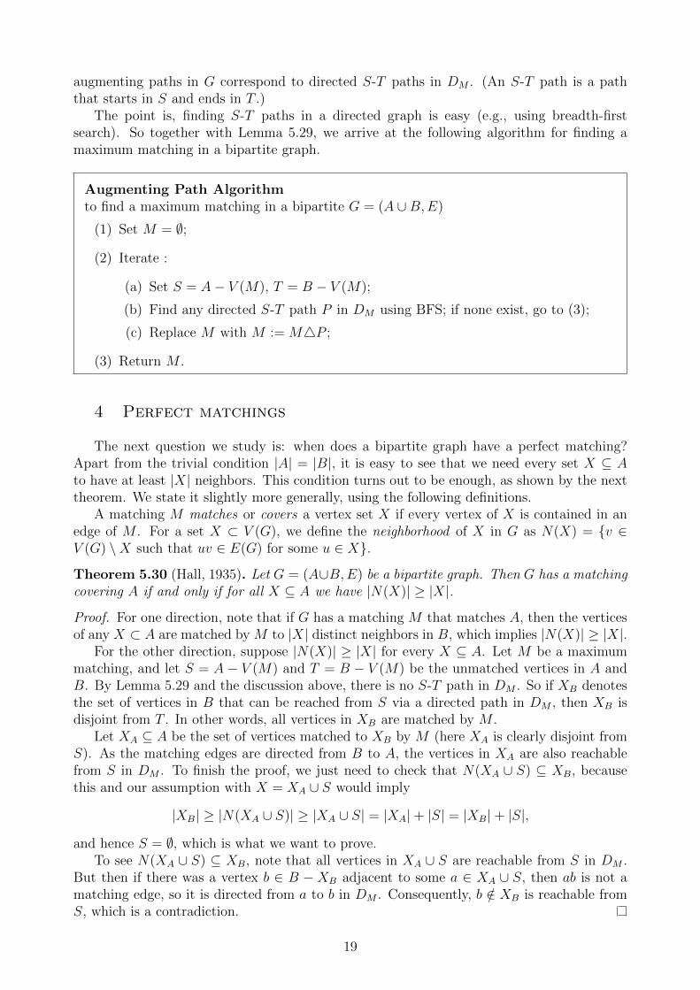
The point is, finding S-T paths in a directed graph is easy (e.g., using breadth-firstsearch). So together with Lemma 5.29, we arrive at the following algorithm for finding amaximum matching in a bipartite graph.

Augmenting Path Algorithmto find a maximum matching in a bipartite G = (A ∪B,E)

(1) Set M = ∅;

(2) Iterate :

(a) Set S = A− V (M), T = B − V (M);

(b) Find any directed S-T path P in DM using BFS; if none exist, go to (3);

(c) Replace M with M := M4P ;

(3) Return M .

4 Perfect matchings

The next question we study is: when does a bipartite graph have a perfect matching?Apart from the trivial condition |A| = |B|, it is easy to see that we need every set X ⊆ Ato have at least |X| neighbors. This condition turns out to be enough, as shown by the nexttheorem. We state it slightly more generally, using the following definitions.

A matching M matches or covers a vertex set X if every vertex of X is contained in anedge of M . For a set X ⊂ V (G), we define the neighborhood of X in G as N(X) = v ∈V (G) \X such that uv ∈ E(G) for some u ∈ X.

Theorem 5.30 (Hall, 1935). Let G = (A∪B,E) be a bipartite graph. Then G has a matchingcovering A if and only if for all X ⊆ A we have |N(X)| ≥ |X|.

Proof. For one direction, note that if G has a matching M that matches A, then the verticesof any X ⊂ A are matched by M to |X| distinct neighbors in B, which implies |N(X)| ≥ |X|.

For the other direction, suppose |N(X)| ≥ |X| for every X ⊆ A. Let M be a maximummatching, and let S = A − V (M) and T = B − V (M) be the unmatched vertices in A andB. By Lemma 5.29 and the discussion above, there is no S-T path in DM . So if XB denotesthe set of vertices in B that can be reached from S via a directed path in DM , then XB isdisjoint from T . In other words, all vertices in XB are matched by M .

Let XA ⊆ A be the set of vertices matched to XB by M (here XA is clearly disjoint fromS). As the matching edges are directed from B to A, the vertices in XA are also reachablefrom S in DM . To finish the proof, we just need to check that N(XA ∪ S) ⊆ XB, becausethis and our assumption with X = XA ∪ S would imply

|XB| ≥ |N(XA ∪ S)| ≥ |XA ∪ S| = |XA|+ |S| = |XB|+ |S|,

and hence S = ∅, which is what we want to prove.To see N(XA ∪ S) ⊆ XB, note that all vertices in XA ∪ S are reachable from S in DM .

But then if there was a vertex b ∈ B − XB adjacent to some a ∈ XA ∪ S, then ab is not amatching edge, so it is directed from a to b in DM . Consequently, b /∈ XB is reachable fromS, which is a contradiction.

19

If |A| = |B|, then of course every matching covering A covers B, as well. So Hall’s theoremimplies that a bipartite graph G = (A∪B,E) has a perfect matching if and only if |A| = |B|and |N(X)| ≥ |X| for every X ⊆ A.

The property “|N(X)| ≥ |X| for every X ⊆ A” is often referred to as Hall’s condition.Testing this property algorithmically is slow, but it turns out to be a convenient thing tocheck in many theoretical applications.

Corollary 5.31. Let k ≥ 1 be a integer. Every k-regular bipartite graph has a perfectmatching.

Proof. Let G = (A ∪ B,E) be a k-regular bipartite graph. Since every edge touches exactlyone vertex of A, and every vertex of A touches exactly k edges, the number of edges in G isexactly k|A|. By a similar argument, the number of edges is exactly k|B|, so k ≥ 1 implies|A| = |B|.

As discussed above, Hall’s condition would now guarantee a perfect matching. To checkit, let X ⊆ A be a vertex set. We will double-count the edges touching X. On the one hand,there are exactly k|X| such edges. On the other hand, every such edge has its other endpointin N(X), so the number of such edges is at most k|N(X)|. Hence k|X| ≤ k|N(X)|, whichagain implies |X| ≤ |N(X)|.

20

Lecture 6

Konig’s theorem. Flows.

1 Konig’s Theorem

Definition. Given a graph G, a vertex cover for G is a set C ⊂ V (G) such that every edgeof G is incident with a vertex in C.

The maximum size of a matching in G is denoted by ν(G), and the minimum size of avertex cover in G is denoted by τ(G). (Note that the “size” of a matching is the number ofedges in it, while the “size” of a vertex cover is the number of vertices in it.)

Theorem 6.32 (Konig, 1931). Let G = (A∪B,E) be a bipartite graph. Then ν(G) = τ(G).

Proof. It is clear that ν(G) ≤ τ(G), because a vertex cover has to cover every edge of thematching with one of the endpoints of the edge. So to cover a matching of size ν(G), we needat least this many vertices.

Now we show ν(G) ≥ τ(G). Let M be a maximum matching of G, and as before, letS = A−V (M) and T = B−V (M) be the set of unmatched vertices. As observed last time,if M is maximum, there is no S-T path in DM .

Let XB be the set of vertices in B that can be reached from S via a (directed) path inDM , and let YA be the set of vertices in A that cannot be reached from S in DM . Clearly,XB is disjoint from T and YA is disjoint from A. Note also, that either both ends of an edgein M can be reached from S, or neither of them can be. In the former case, the edge has anend vertex in XB, in the latter case it has an endpoint in YA. Consequently, |XB ∪YA| = |M |

We will now show that XB ∪ YA is a vertex cover. Suppose not, then there is an edge uvwith u ∈ A and v ∈ B not covered by this set (i.e., u /∈ YA and v /∈ XB). But uv is not amatching edge, so in DM , it is directed from u to v. But then u ∈ A − YA can be reachedfrom S in DM (by definition), so v should also be reachable via the edge uv. This contradictsv /∈ XB.

So XB ∪ YA is a vertex cover of size ν(G), implying ν(G) ≥ τ(G).

2 Flows

Definition. A network is a directed graph G = (V,E) with two special vertices, the sources ∈ V and the sink t ∈ V , together with a non-negative capacity function c : E → R.

Definition. A flow in a network G = (V,E) is a function f : V 2 → R such that

1. (flow conservation) for every v ∈ V − s, t,∑w∈V

f(v, w) =∑w∈V

f(w, v)

2. (capacity constraint) 0 ≤ f(u, v) ≤ c(u, v) for every −→uv ∈ E

3. f(u, v) = 0 if −→uv 6∈ E.

21

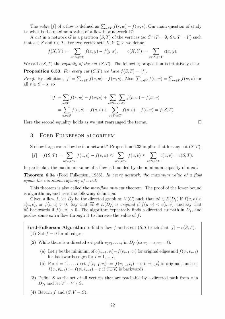
The value |f | of a flow is defined as∑

w∈V f(s, w)− f(w, s). Our main question of studyis: what is the maximum value of a flow in a network G?

A cut in a network G is a partition (S, T ) of the vertices (so S ∩ T = ∅, S ∪ T = V ) suchthat s ∈ S and t ∈ T . For two vertex sets X, Y ⊆ V we define

f(X, Y ) :=∑

x∈X,y∈Y

f(x, y)− f(y, x), c(X, Y ) :=∑

x∈X,y∈Y

c(x, y).

We call c(S, T ) the capacity of the cut (S, T ). The following proposition is intuitively clear.

Proposition 6.33. For every cut (S, T ) we have f(S, T ) = |f |.Proof. By definition, |f | =

∑w∈V f(s, w)− f(w, s). Also,

∑w∈V f(v, w) =

∑w∈V f(w, v) for

all v ∈ S − s, so

|f | =∑w∈V

f(s, w)− f(w, s) +∑v∈S−s

∑w∈V

f(v, w)− f(w, v)

=∑u,v∈S

f(u, v)− f(u, v) +∑

u∈S,v∈T

f(u, v)− f(v, u) = f(S, T )

Here the second equality holds as we just rearranged the terms.

3 Ford-Fulkerson algorithm

So how large can a flow be in a network? Proposition 6.33 implies that for any cut (S, T ),

|f | = f(S, T ) =∑

u∈S,v∈T

f(u, v)− f(v, u) ≤∑

u∈S,v∈T

f(u, v) ≤∑

u∈S,v∈T

c(u, v) = c(S, T ).

In particular, the maximum value of a flow is bounded by the minimum capacity of a cut.

Theorem 6.34 (Ford–Fulkerson, 1956). In every network, the maximum value of a flowequals the minimum capacity of a cut.

This theorem is also called the max-flow min-cut theorem. The proof of the lower boundis algorithmic, and uses the following definition.

Given a flow f , let Df be the directed graph on V (G) such that −→uv ∈ E(Df ) if f(u, v) <c(u, v), or f(v, u) > 0. Say that −→uv ∈ E(Df ) is original if f(u, v) < c(u, v), and say that−→uv backwards if f(v, u) > 0. The algorithm repeatedly finds a directed s-t path in Df , andpushes some extra flow through it to increase the value of f .

Ford-Fulkerson Algorithm to find a flow f and a cut (S, T ) such that |f | = c(S, T ).

(1) Set f = 0 for all edges;

(2) While there is a directed s-t path v0v1 . . . vl in Df (so v0 = s, vl = t):

(a) Let ε be the minimum of c(vi−1, vi)−f(vi−1, vi) for original edges and f(vi, vi−1)for backwards edges for i = 1, ..., l.

(b) For i = 1, . . . , l set f(vi−1, vi) := f(vi−1, vi) + ε if −−−→vi−1vi is original, and setf(vi, vi−1) := f(vi, vi−1)− ε if −−−→vi−1vi is backwards.

(3) Define S as the set of all vertices that are reachable by a directed path from s inDf , and let T = V \ S.

(4) Return f and (S, V − S).

22

We verify that the algorithm works correctly if c is integer valued. First, note that fsatisfies the three conditions in the definition of a flow at each step. Second, since in thenetwork all capacities are integral, we have that ε > 0 is an integer at each step, and so ε ≥ 1.Therefore, since the flow must be finite (bounded by the capacity of any cut), the algorithmterminates in a finite number of steps. Finally, by the definition of Df and the set S, wehave f(u, v) = c(u, v) for every edge −→uv with u ∈ S, v ∈ T , and f(v, u) = 0 for every edge −→vuwith u ∈ S, v ∈ T . Hence

f(S, T ) =∑

u∈S,v∈T

f(u, v)− f(v, u) =∑

u∈S,v∈T

c(u, v) = c(S, T ).

Since ε is always an integer, we even get the following.

Fact 6.35. If c is integral, then there is an integer maximum flow.

Note that for the algorithm to stop, it was important that c takes integer values. Thesame argument works for rational c, as well (e.g., by multiplying all values with a number tomake c integral), but the algorithm might not stop if c has non-rational values (see problemset). However, Theorem 6.34 holds for any non-negative real capacity function. This canbe proved by approximating it with a rational function and taking the limit. Alternatively,Edmonds and Karp showed that the algorithm stops in a bounded number of steps no matterwhat the capacity function is, provided that it chooses the shortest s-t path of Df in step 2.

Let us give a quick application of the Ford-Fulkerson theorem.

Application: Proof of Theorem 6.32 via Ford-Fulkerson.Given G = (A ∪ B,E), let us create a network by adding a source s that sends an edge ofcapacity 1 to all vertices of A, and adding a sink t that receives an edge of capacity 1 fromall vertices of B. We also orient the edges of G from A to B give them infinite capacities.(Think of ∞ as some large number bigger than |A|.)

Let f be an integer maximum flow. We claim that the G-edges with positive flow form amatching. Indeed, each such edge has f(u, v) ≥ 1. If two such edges shared a vertex u ∈ A,then the inflow at u is at most 1 and the outflow is at least 2, which is not possible. Similarly,two such edges cannot meet in B, either. Hence ν(G) ≥ |f |.

Now let (S, T ) be a minimum cut. Then (S ∩B)∪ (T ∩A) is a vertex cover, because anyuncovered edge (u, v) with u ∈ S ∩A and v ∈ T ∩B would contribute ∞ capacity to c(S, T )(but c(S, T ) ≤ C(s, V − s) ≤ |A| <∞). Here every s-(T ∩A) edge and every (S ∩B)-t edgecontributes 1 to c(S, T ), so we get τ(G) ≤ |S ∩B|+ |T ∩ A| ≤ c(S, T ). Hence

τ(G) ≤ c(S, T ) = |f | ≤ ν(G),

which, together with the trivial ν(G) ≤ τ(G) finishes the proof.

s t

1

1 ∞

∞1

1

23

Lecture 7

Tutte polynomial.

For now, please consult https://piazza.com/class/k0o1x6oxrsa7cr?cid=17

24

Lecture 8

Coloring.

2 Vertex coloring

Recall the we call a graph (properly) k-colorable if its vertices can be colored with kcolors in such a way that no two adjacent vertices get the same color, and that the chromaticnumber χ(G) is the minimum k such that G is k-colorable.

So far we have looked at the chromatic number of planar graphs, but it also makes senseto study the concept for general graphs. Actually, many real-life problems may be interpretedas graph coloring problems. Here is one example from scheduling:

Example. The students at a certain university have annual examinations in all the coursesthey take. Naturally, examinations in different courses cannot be held concurrently if thecourses have students in common. How can all the examinations be organized in as fewparallel sessions as possible? To find a schedule, consider the graph G whose vertex setis the set of all courses, two courses being joined by an edge if they give rise to a conflict.Clearly, independent sets of G correspond to conflict-free groups of courses. Thus, the requiredminimum number of parallel sessions is the chromatic number of G.

We first collect some easy facts about the chromatic number.

Definition. The complement of a graph G is the graph G with vertex set V (G) = V (G) andedge set E(G) = xy : x, y ∈ V (G), xy 6∈ E(G).The clique number ω(G) is the size of the largest complete subgraph (clique) of G. So ω(G) =α(G).

Fact 8.36. 1. χ(Ks) = s

2. G is bipartite if and only if χ(G) ≤ 2

3. If H is a subgraph of G, then χ(H) ≤ χ(G)

4. χ(G) ≥ ω(G) for every graph G.

Proof. 1. and 2. follow from the definition. For 3., we just need to notice that every propercoloring of G provides a coloring of H. 4. is then a combination of 1. and 3.

So ω(G) is a trivial lower bound on the chromatic number, but it is not necessarily tight:

Example. The following graph G satisfies χ(G) = 4 and ω(G) = 3.

G =

In general, the chromatic number cannot be bounded by any function of the clique number.We show two different constructions of graphs with no triangle and arbitrarily large chromaticnumber.

25

Theorem 8.37. For every positive integer k, there exists a graph Gk with ω(G) = 2 andχ(G) ≥ k

Proof. Construction 1. We prove this by induction on k. For k = 2, we can take G2 be asingle edge.

Now suppose that k ≥ 3. Let H1, ..., Hk−1 be k − 1 disjoint copies of Gk−1. For everyv1 ∈ V (H1), . . . , vk−1 ∈ V (Hk−1), add a vertex X(v1, ..., vk−1) that is only connected tov1, ..., vk−1, and let Gk be the resulting graph.

Clearly, ω(Gk) = 2. Indeed, Hi does not contain a triangle, so if there exists a trianglein Gk, then one of its vertices is X(v1, ..., vk−1) for some selection vi ∈ Hi. But vi and vj arenot neighbors for i 6= j, so X(v1, ..., vk−1) cannot be contained in a triangle either.

Now we show that χ(Gk) ≥ k. Suppose that there exists a proper coloring c : V (Gk) →1, ..., k − 1. As χ(Hi) ≥ k − 1, every color must appear in Hi. But then let vi ∈ V (Hi)such that c(vi) = i. Then every color was used in the neighborhood of X(v1, ..., vk−1),contradiction.

Construction 2. Let n ≥ 2k. The shift graph Sn is the graph with vertex set

(i, j) : 1 ≤ i < j ≤ n,

where (i, j) and (k, l) are joined by an edge if j = k. Clearly, ω(Sn) = 2.Let c : V (Sn)→ X be a proper coloring of Sn. For i ∈ 1, ..., n, let

Xi = c((i, j)) : i ≤ j ≤ n,

that is, Xi is the set of colors used for the vertices (i, i+ 1), ..., (i, n). The main observationis that if i 6= j, then Xi 6= Xj. Otherwise, if Xi = Xj, then consider the color c = c((i, j)).By definition, c ∈ Xi, but then c ∈ Xj, which means that there exists j < k ≤ n such thatc((j, k)) = c. But (i, j) and (j, k) are neighbors of the same color, contradiction.

As there are 2|X| different subsets of X, and X1, ..., Xn are pairwise different, we musthave 2|X| ≥ n, which gives |X| ≥ log2 n ≥ k.

A k-coloring can be thought of splitting the vertices into k independent sets. This readilyimplies the following lower bound on χ(G).

Lemma 8.38. For every graph G, we have χ(G) ≥ |V (G)|α(G)

.

Proof. Given a coloring with χ(G) colors, the color classes (label them V1, . . . , Vχ(G)) areindependent sets, and thus have size at most α(G). Hence we have

|V (G)| =χ(G)∑i=1

|Vi| ≤χ(G)∑i=1

α(G) = χ(G)α(G).

Claim 8.39. For any two graphs G1 and G2 on the same vertex set V , χ(G1 ∪ G2) ≤χ(G1)χ(G2).

Proof. For both i = 1, 2, let ki = χ(Gi) and take a ki-coloring ci : V → [ki] of Gi. (Here[n] denotes the set 1, . . . , n.) We will color the vertices in V with elements of the set[k1]× [k2]. Indeed, c(v) = (c1(v), c2(v)) gives a proper k1k2-coloring of G = G1 ∪G2, becauseif two vertices u, v are adjacent in G, then they are also adjacent in some Gi, hence the i’thcoordinate of their colors will differ. So χ(G) ≤ k1k2.

26

Further simple bounds on the chromatic number can be found in the problem set.

Let G = (V,E) be a graph. We say that G is d-degenerate if every subgraph of G has avertex of degree less than or equal to d. The following proposition connects the degeneracyof G and the chromatic number of G. The six color theorem was in fact a special case of thislemma.

Lemma 8.40. If G is d-degenerate, then χ(G) ≤ d+ 1.

Proof. We do induction on the number of vertices. The statement is clearly true for all Gwith at most d + 1 vertices. For larger graphs, pick a vertex v of degree ≤ d in G. Thegraph G− v is d-degenerate (because every subgraph of G− v is a subgraph of G), so it canbe (d+ 1)-colored. Then color v into the color that does not appear among the colors of itsneighbors. This gives a proper coloring of G.

Corollary 8.41. χ(G) ≤ ∆(G) + 1 for every graph G.

Proof. G is clearly ∆(G)-degenerate.

This corollary is tight for cliques and odd cycles. Interestingly, those are basically theonly examples, as shown by the following theorem.

Theorem 8.42 (Brooks, 1941). Let G be a connected graph that is not isomorphic to Ks orC2k+1 for any s or k. Then χ(G) ≤ ∆(G).

We will not prove this theorem.

3 Edge coloring

Definition. A proper edge coloring of a graph G is a map c : E(G) → X for some setof colors X, such that c(e) 6= c(e′) whenever e, e′ are distinct edges that share a vertex.The edge-chromatic number χ′(G) of G is the minimum size of such a set X, i.e., it is theminimum number k such that the G can be (properly) k-edge-colored.

Example.

• χ′(K3) = 3

• χ′(C4) = 2

• χ′(K4) = 3

• The picture on the right is an edge col-oring of the Petersen graph with fourcolors. It is not difficult to see that itsedge chromatic number is equal to 4.

Definition. A matching M is a set of vertex-disjoint edges, i.e., a set of edges such that notwo of them share an endvertex.

Each color class is a set is a matching, so an edge coloring is a partition of the edges intomatchings.

Lemma 8.43. For any graph G with at least one edge we have ∆(G) ≤ χ′(G) ≤ 2∆(G)− 1.

27

Proof. There is vertex of degree ∆(G), and an edge coloring must give different colors toeach of the ∆(G) edges at that vertex. This implies χ′(G) ≥ ∆(G).

The upper bound follows by a proof similar to the proof of Lemma 8.40: We can doinduction on the number of edges. So delete an edge e, and take a (2∆(G)− 1)-edge-coloringof G− e. Since an edge shares a vertex with at most 2(∆(G)− 1) edges, there must be a freecolor left for e.

However, this simple upper bound can be significantly improved. This is shown by thefollowing theorem, which tells us that any graph G has edge-chromatic number either ∆(G)or ∆(G) + 1. Both are possible, since even cycles have χe(G) = ∆(G) and odd cycles haveχe(G) = ∆(G) + 1. However, the algorithm in the proof still does not always give the exactnumber, and in fact it is NP-hard to determine which of the two values is the edge-chromaticnumber of a given graph.

Theorem 8.44 (Vizing, 1964). For every graph G we have χ′(G) = ∆ or ∆(G) + 1.

Proof. We only need to show χ′(G) ≤ ∆(G) + 1. To prove this, we use induction on thenumber of edges. The statement clearly holds for a graph without edges.

Given an edge xy ∈ E(G), we describe an algorithm that, given an edge coloring of G−xywith at most ∆(G) + 1 colors, produces an edge coloring of G with this many colors. But tofind a color for xy, the algorithm may have to change the colors of other edges.

So take a coloring of G− xy. As there are more than ∆(G) available colors, every vertexhas at least one color missing from the edges touching it. We say that a vertex v is c-free, ifno edge incident to v has color c.

Now let us build a fan of edges around x as follows. Take the edge xy, and let y0 = y.We know that y0 is c1-free for some color c1. Now let xy1 be an edge of color c1, if such anedge exists. Then y1 is c2-free for some color c2.

Continue similarly: if there is an edge at x of color ci that we have not looked at, let xyibe this edge, and let ci+1 be a color missing at yi. We repeat this process until we can; letxyk be the last edge we added. There are two possible reasons for getting stuck: either thereis no edge at x of color ck+1, or this edge already appeared at some previous xyi.

Case 1. x is ck+1-free.In this case we can just “rotate” the colors around x: Define the new color of xyi to be

ci+1 for every i = 0, . . . , k (keeping the colors of all other edges). This does not create anyissue with any yi, because it had been ci+1-free. There is no problem at x either, because theonly new color introduced is ck+1. Hence this is a proper coloring of G (including the edgexy = xy0).

Case 2. x is not ck+1-free.As noted above, the maximality of k implies that some edge xyi is ck+1-colored, so by

definition ck+1 = ci. Let us just call this color c, and let d be a color such that x is d-free.Now let P be a maximal path starting at x that only uses the colors c and d. Actually,

since every vertex touches at most one c-colored and one d-colored edge, and x is d-free, thereis a unique such maximal path P = xyi . . . z for some vertex z. Let us swap the colors cand d along the path. The same observation shows that this is still a proper edge-coloring ofG− e. We again distinguish two cases.

Case 2/A. z = yi−1.Note that yi−1 was c-free, so the last edge of P must have had color d. After swapping,

yi−1 is no longer c-free, but it is now d-free. However, the edge xyi has color d, as well, sothe edges xyi satisfy the required properties with ci = d now. As x is now c-free, we arrive

28

at a situation covered by Case 1, which gives a proper coloring of G (by rotating the colors,i.e., coloring each xyj with color cj+1).

Case 2/B. z 6= yi−1.In this case, yi−1 remains c-free, and x becomes c-free, as well. This means that we can

rotate the colors on the first i edges only to get a proper edge coloring: recolor xyj with thecolor cj+1 for every j = 0, . . . , i− 1, and leave the color of other edges the same as what wehad after swapping c and d along P . By the same arguments as before, every edge is colored,but no two touching edges get the same color.

29

Lecture 9

Connectivity.

1 Menger’s theorem

Next we will look at what the Ford-Fulkerson theorem says about networks where everyedge has capacity 1. The results in this section hold for directed and undirected graphs, aswell. We use the following notation: if G = (V,E) is a graph and W ⊆ V, F ⊆ E, thenG −W is the graph with vertex set V \W and edge set E \ e ∈ E : e ∩W 6= ∅, and thegraph G \ F is the graph with vertex set V and edge set E \ F .

Definition. Let G = (V,E) be a (directed) graph, and s, t ∈ V .We say that two paths from s to t (s-t paths) in G are edge-disjoint, if they don’t share

any edges. We say that they are internally vertex-disjoint, if they don’t share any verticesother than s and t.

A subset F ⊆ E is an s-t edge separator, if G−F contains no s-t path. A subset W ⊆ Vis an s-t vertex separator, if G−W contains no s-t path.

The following theorem is one of the cornerstones of graph theory.

Theorem 9.45 (Menger). In a (directed) graph G = (V,E) with s, t ∈ V :

1. Maximum number of edge-disjoint s-t paths = minimum size of an s− t edge separator.

2. If (s, t) /∈ E, then:Max number of internally vertex-disjoint s-t paths = min size of an s−t vertex separator.

Proof. “≤” is clear in both statements: To “destroy” all the s-t paths, we need to delete adistinct edge/vertex from each of them. So any separator has size at least the number ofpaths.

Now we show “≥” for directed G.

1. Take the network on G where all edges have capacity 1. We will prove

max # s-t edge-disjoint paths ≥ max flow = min cut ≥ min s-t edge separator

For the first inequality, take a maximum integer flow f . If |f | > 0, then there is ans-t path P using flow edges. Removing P from f decreases the value of f by 1. Moreprecisely, we “push back” a capacity-1 flow on P to decrease |f | by 1. Crucially, as allcapacities are 1, the new flow does not use any edge of P . So if we repeat this step |f |times, we get |f | edge-disjoint s-t paths, just what we wanted.

The equality in the middle is just the max-flow min-cut theorem (Theorem 6.34). Forthe last inequality, note that the edges appearing in a min cut form an s-t edge sepa-rator. As the edge capacities are all 1, the capacity of this cut is exactly the numberof edges in the edge separator.

2. The key to ensure edge-disjointness in the first statement was to limit the edge capacitiesto 1. To limit the capacities of vertices, we need a trick. Let us define the network Gbased on G as follows:

30

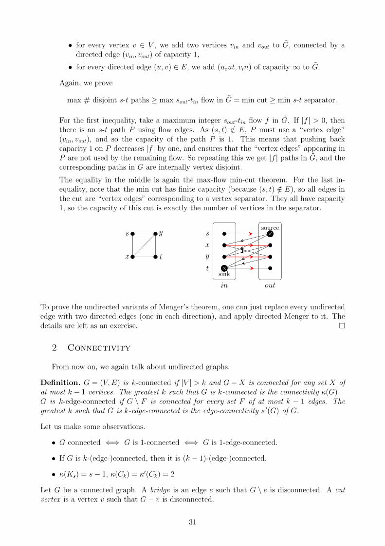
• for every vertex v ∈ V , we add two vertices vin and vout to G, connected by adirected edge (vin, vout) of capacity 1,

• for every directed edge (u, v) ∈ E, we add (uout, vin) of capacity ∞ to G.

Again, we prove

max # disjoint s-t paths ≥ max sout-tin flow in G = min cut ≥ min s-t separator.

For the first inequality, take a maximum integer sout-tin flow f in G. If |f | > 0, thenthere is an s-t path P using flow edges. As (s, t) /∈ E, P must use a “vertex edge”(vin, vout), and so the capacity of the path P is 1. This means that pushing backcapacity 1 on P decreases |f | by one, and ensures that the “vertex edges” appearing inP are not used by the remaining flow. So repeating this we get |f | paths in G, and thecorresponding paths in G are internally vertex disjoint.

The equality in the middle is again the max-flow min-cut theorem. For the last in-equality, note that the min cut has finite capacity (because (s, t) /∈ E), so all edges inthe cut are “vertex edges” corresponding to a vertex separator. They all have capacity1, so the capacity of this cut is exactly the number of vertices in the separator.

×

×s

tx

y s

x

y

t

in out

source

sink

To prove the undirected variants of Menger’s theorem, one can just replace every undirectededge with two directed edges (one in each direction), and apply directed Menger to it. Thedetails are left as an exercise.

2 Connectivity

From now on, we again talk about undirected graphs.

Definition. G = (V,E) is k-connected if |V | > k and G−X is connected for any set X ofat most k − 1 vertices. The greatest k such that G is k-connected is the connectivity κ(G).G is k-edge-connected if G \ F is connected for every set F of at most k − 1 edges. Thegreatest k such that G is k-edge-connected is the edge-connectivity κ′(G) of G.

Let us make some observations.

• G connected ⇐⇒ G is 1-connected ⇐⇒ G is 1-edge-connected.

• If G is k-(edge-)connected, then it is (k − 1)-(edge-)connected.

• κ(Ks) = s− 1, κ(Ck) = κ′(Ck) = 2

Let G be a connected graph. A bridge is an edge e such that G \ e is disconnected. A cutvertex is a vertex v such that G− v is disconnected.

31

• G is 2-connected ⇐⇒ G has no cut vertex.G is 2-edge-connected ⇐⇒ G has no bridge.

Theorem 9.46 (Global version of Menger’s theorem). Let G = (V,E) be a graph.

1. G is k-edge-connected ⇐⇒ G contains k edge-disjoint paths between any two vertices

2. G is k-connected ⇐⇒ G contains k internally vertex-disjoint paths between any twovertices

This is a strong characterization of k-connected graphs that easily implies the followingnon-trivial facts.

Proposition 9.47. κ(G) ≤ κ′(G) ≤ δ(G).

Proof. κ′(G) ≤ δ(G) is trivial, because deleting all edges touching a vertex disconnects G.To show κ(G) ≤ κ′(G), note that by Theorem 9.46, any two vertices of G are connected

by κ(G) internally vertex-disjoint paths. But then these paths are edge-disjoint, so any twovertices are connected by κ(G) edge-disjoint paths, hence G is κ(G)-edge-connected by theother direction of Theorem 9.46.

Proposition 9.48. G is 2-connected ⇐⇒ any 2 vertices of G are on a cycle.

Proof. By Theorem 9.46, G is 2-connected if and only if any two vertices are connected by2 internally vertex-disjoint paths. But this happens if and only if the two vertices are on acycle (the union of the two paths).

Proof of Theorem 9.46. After the local version, this is not hard to prove.

1. ⇐: If s and t are connected by k edge-disjoint paths, any s-t edge-separator needs tocontain at least one edge from each path. As this is true for any pair of vertices, there isno set F of at most k− 1 edges such that deleting F disconnects G, thereby separatingsome two vertices.

⇒: If G is k-edge-connected, then there is smallest s-t edge separator has size at leastk for every s, t ∈ V . Then by Theorem 9.45, s and t are connected by k edge-disjointpaths for any s, t ∈ V .

2. ⇐: The above argument works the same with vertices instead of edges.

⇒: Again the same argument works, except for adjacent pairs s, t ∈ V . The problemis that we cannot apply Menger’s theorem if st ∈ E. We fix this issue by deleting it,so let G′ = G \ st.

Claim. G′ is (k − 1)-connected.

Proof of Claim. Suppose not, i.e., there is a set X of at most k − 2 vertices such thatG′ −X is disconnected. Note that G−X is not disconnected (G is k-connected), andG′ − X = (G − X) \ st, so s and t must be in different components of G′ − X. Nowas G is k-connected, it has at least k + 1 vertices, so there is a vertex w not in X anddifferent from s, t. We may assume that w and t are in different components of G′−X(if not, then w and s are). But then X ′ = X ∪ s is a set of k − 1 vertices such thatG−X = G′−X (because deleting s deletes the edge st), and so G−X is disconnected.This contradicts G being k-connected.

32

Using this claim, we can apply Theorem 9.45 to G′ and get k − 1 internally vertex-disjoint s-t paths in G′. Together with the edge st, we get k such paths in G, as needed.All we have left is to prove this claim.

The following corollary of the global Menger’s theorem, called the fan lemma, is a niceand highly applicable tool for k-connected graphs.

Lemma 9.49 (fan lemma). Let G be a k-connected graph. For every x ∈ V (G) and U ⊆V (G) with |U | ≥ k, there are k paths from x to U that are disjoint aside from x, and eachhas exactly one vertex in U .

Proof. Add a vertex u that is adjacent to all the vertices in U . It is an easy exercise tocheck that the resulting graph is still k-connected (note that this requires |U | ≥ k). ByTheorem 9.46, there are k internally vertex-disjoint paths from x to u. Removing u fromthese paths gives paths from x to U that are disjoint aside from x. If such a path touchesmore than one vertex in U , then it contains a subpath with exactly one vertex from U , whichwe can take instead.

33

Lecture 10

The probabilistic method.

Probabilistic tools turn out to be extremely useful for certain combinatorial problems. Atfirst, applications might feel like magic: problems that have nothing to do with probabilityoften have simple solutions if we introduce some randomness. Deeper theoretical results (likethe so-called Szemeredi regularity lemma) show some inherent connection between graphsand random structures.

However, (fortunately or unfortunately) this is not the course to go this deep, so we willhave to stick with the magical results.

1 Review of basic notions

We will use standard notions from probability theory, although in a quite restricted set-ting: we will always work with a probability space that is defined on a finite base set Ω witha probability mass function p : Ω→ [0, 1] satisfying

∑ω∈Ω p(ω) = 1. The events in this prob-

ability space are all subsets E ⊆ Ω, and the probability that E holds is P[E] =∑

ω∈A p(ω).A random variable is just a function X : Ω→ R, and the expected value or expectation of

a random variable X is

E[X] =∑x∈R

x · P[X = x] =∑ω∈Ω

p(ω) ·X(ω).

A very important fact (that can be easily seen from the right-hand side of this equality) isthe linearity of expectation, i.e., that for any two random variables X and Y and any real c,we have E[X + Y ] = E[X] + E[Y ] and E[cX] = cE[X].

Two events E1 and E2 are said to be independent if P[E1 ∩E2] = P[E1] · P[E2]. For morethan two events, E1, . . . , Ek are independent if for any I ⊆ 1, . . . , k, we have

P

[⋂i∈I

Ei

]=∏i∈I

P[Ei].

Similarly, the random variables X1, . . . , Xk are independent if for any x1, . . . , xk and anyI ⊆ 1, . . . , k, we have

P

[⋂i∈I

Xi = xi

]=∏i∈I

P[Xi = xi].

2 Simple applications

As a first example, let us give a new proof of the following fact. In Lecture 2, we gave analgorithmic proof, this time we provide a probabilistic argument.

Proposition 10.50. Any graph G contains a bipartite subgraph H with |E(H)| ≥ |E(G)|/2.

Proof. Let us take a random partition of the vertices into parts A and B, where each vertexis independently assigned to A or B with probability 1/2. So Ω is the set of all partitions. Forevery edge e ∈ E(G), let Xe be the indicator random variable for the event that e “crosses”

34

between A and B. Then X =∑

e∈E(G) Xe is a random variable that counts the number ofedges crossing between A and B. Thus the expected number of edges crossing is

E[X] = E

[∑e∈E

Xe

]=∑e∈E

E[Xe].

Here for an edge e = uv, we have

E[Xe] = P[e crossing] = P[u ∈ A, v ∈ B] + P[u ∈ B, v ∈ A] =1

2· 1

2+

1

2· 1

2=

1

2,

so E[X] =∑

e∈E 1/2 = |E(G)|/2. But then there must be a partition ω ∈ Ω such thatX(ω) ≥ |E(G)|/2 (otherwise the expectation would be strictly smaller).

Note that this is only an existence proof. We do not get any information on how to findsuch a subgraph.

For our next application, we give a new proof of the quantitative version of Turan’stheorem. As a reminder, Turan’s theorem implies that ex(n,Kr) ≤ (1 − 1

r−1)n

2

2. Taking

graph complementation, this implies that if G is a graph with less than(n

2

)−(

1− 1

r − 1

)n2

2=

n2

2(r − 1)− n

2

edges, then G has an independent set of size r. In other words, if G is a graph with n verticesand e edges, then α(G) ≥ n2

2e+n. We shall prove this equivalent formulation of Turan’s

theorem, and we will deduce this from an even stronger theorem, which takes the degreesequence of the graph in consideration.

Theorem 10.51. (Caro) Let G be a graph. Then G contains an independent set of size atleast ∑

v∈V (G)

1

1 + d(v).

Proof. Let n = |V (G)| and let v1, ..., vn be a random ordering of the vertex set, that is, anordering chosen from the set of all possible ordering with probability 1/n!. Let S be the setof vertices vi such that vi has no neighbor in v1, ..., vi−1. Then S is an independent set.Let us calculate the expected value of the size of S.

For a vertex v, let Xv be the indicator random variable that v is in S. That is, Xv = 1 ifv ∈ S, Xv = 0, otherwise. Then |S| =

∑v∈V (G) Xv. Also, the probability of the event v ∈ S

is exactly 11+d(v)

, as v ∈ S if v is the first vertex in the ordering among v ∪ N(v). Hence,

E(Xv) = 11+d(v)

. But then by the linearity of expectation, we have

E(|S|) =∑

v∈V (G)

E(Xv) =∑

v∈V (G)

1

1 + d(v).

But then there exists an ordering of the vertices such that |S| ≥∑

v∈V (G)1

1+d(v)and we

are done.

Corollary 10.52. Let G be a graph with n vertices and e edges. Then

α(G) ≥ n2

2e+ n.

35

Proof. By the inequality between the arithmetic and harmonic mean, we have∑v∈V (G)

11+d(v)

n≥ n∑

v∈V (G) 1 + d(v)=

n

2e+ n.

But then α(G) ≥∑

v∈V (G)1

1+d(v)≥ n2

2e+n.

3 Constructions for the Kovari-Sos-Turan theorem

By the Kovari-Sos-Turan theorem, for every positive integer s ≥ 2, we have

ex(n,Ks,s) ≤ cn2−1/s,

where c > 0 is a constant depending only on s. However, if s ≥ 4, it is not known whetherex(n,Ks,s) ≥ c′n2−1/s also hold with some constant c′ > 0, and this is one of the central openquestions in extremal graph theory. In this section, we use the probabilistic method to findgraphs with slightly less than n2−1/s edges that do not contain Ks,s.

Theorem 10.53. Let s ≥ 2 be a positive integer. Then

ex(n,Ks,s) >1

16n2−2/(s+1).

Proof. Let p = 12n−2/(s+1) and let G be the random graph on an n element vertex set in which

each pair of vertices is connected by an edge independently with probability p. The graph Gmight contain Ks,s, but we can make it Ks,s-free by deleting an edge from each copy of Ks,s.Let X be the number of copies of Ks,s in G, more precisely, the number of pairs (A,B) suchthat A,B ⊂ V (G), |A| = |B| = s, A ∩B = ∅ and ab ∈ E(G) for every a ∈ A, b ∈ B.

Let us calculate the expectation of X. For any pair (A,B) such that A,B ⊂ V (G),|A| = |B| = s, A ∩ B = ∅, let XA,B be the indicator random variable that ab ∈ E(G)for every a ∈ A, b ∈ B. Then X =

∑XA,B. The probability that ab ∈ E(G) for every

a ∈ A, b ∈ B is ps2, as this is the probability that s2 given edges are present in G. Hence,

E(XA,B) = ps2. The number of pairs (A,B) such that A,B ⊂ V (G), |A| = |B| = s, A∩B = ∅

is(ns

)(n−ss

)< n2s. By the linearity of expectation, we get

E(X) =∑

E(XA,B) ≤ n2sps2

=1

2s2n2−2/(s+1).

Let Y be the number of edges of G. Then E(Y ) =(n2

)p > 1

4n2p = 1

8n2−2/(s+1).

Consider the random variable Z = Y −X. We have

E(Z) = E(Y )− E(X) =1

8n2−2/(s+1) − 1

2s2n2−2/(s+1) ≥ 1

16n2−2/(s+1),

so there exists a graph G satisfying Z(G) ≥ 116n2−2/(s+1). Remove an arbitrary edge from

each copy of Ks,s in G and let H be the resulting graph. Then H is Ks,s-free, and ss weremoved at most X(G) edges, we have E(H) ≥ Y (G)−X(G) = Z(G) ≥ 1

16n2−2/(s+1).

36