gradient-enhanced kriging for high-dimensional problemsgradient-enhanced kriging for...
TRANSCRIPT

Gradient-enhanced kriging for high-dimensional problems
Mohamed A. [email protected]
Joaquim R. R. A. [email protected]
August 10, 2017
Abstract
Surrogate models provide a low computational cost alternative to evaluating expensivefunctions. The construction of accurate surrogate models with large numbers of independentvariables is currently prohibitive because it requires a large number of function evaluations.Gradient-enhanced kriging has the potential to reduce the number of function evaluationsfor the desired accuracy when efficient gradient computation, such as an adjoint method, isavailable. However, current gradient-enhanced kriging methods do not scale well with thenumber of sampling points due to the rapid growth in the size of the correlation matrixwhere new information are added for each sampling point in each direction of the designspace. They do not scale well with the number of independent variables either due to theincrease in the number of hyperparameters that needs to be estimated. To address this issue,we develop a new gradient-enhanced surrogate model approach that drastically reduced thenumber of hyperparameters through the use of the partial-least squares method that maintainsaccuracy. In addition, this method is able to control the size of the correlation matrix byadding only relevant points defined through the information provided by the partial-leastsquares method. To validate our method, we compare the global accuracy of the proposedmethod with conventional kriging surrogate models on two analytic functions with up to 100dimensions, as well as engineering problems of varied complexity with up to 15 dimensions.We show that the proposed method requires fewer sampling points than conventional methodsto obtain a desired accuracy, or provides more accuracy for a fixed budget of sampling points.In some cases, we get over 3 times more accurate models than a bench of surrogate modelsfrom the literature, and also over 3200 times faster than standard gradient-enhanced krigingmodels.
1
arX
iv:1
708.
0266
3v1
[cs
.LG
] 8
Aug
201
7

Symbols and notation
Matrices and vectors are in bold type.
Symbol Meaning
d Number of dimensionsB Hypercube expressed by the product between intervals of each direction spacen Number of sampling pointsh Number of principal componentsx, x′ 1× d vectorxj jth element of x for j = 1, . . . , dX n× d matrix containing sampling pointsy n× 1 vector containing simulation of Xx(i) ith sampling point for i = 1, . . . , n (1× d vector)y(i) ith evaluated output point for i = 1, . . . , nX(0) XX(l−1) Matrix containing residual of the (l − 1)th inner regressionk(·, ·) Covariance functionrxx′ Spatial correlation between x and x′
R Covariance matrixs2(x) Prediction of the kriging varianceσ2 Process varianceθi jth parameter of the covariance function for i = 1, . . . , dY (x) Gaussian process1 n-vector of onestl lth principal component for l = 1, . . . , hw Weight vector for partial least squares∆xj First order Taylor approximation step in the jth direction
1 Introduction
Surrogate models, also known as metamodels or response surfaces, consist in approximate functions(or outputs) over a space defined by independent variables (or inputs) based on a limited number offunction evaluations (or samples). The main motivation for surrogate modeling is to replace expen-sive function evaluations with the surrogate model itself, which is much less expensive to evaluate.Surrogate model approaches often used in engineering applications include polynomial regression,support vector machine, radial basis function models, and kriging [Forrester et al., 2008]. Surrogatemodels are classified based on whether they are non-interpolating, such as polynomial regression,or interpolating, such as kriging. Surrogate models can be particularly helpful in conjunctionwith numerical optimization, which requires multiple function evaluations over a design variablespace [Haftka et al., 2016; Jones, 2001; Simpson et al., 2001b]. However, non-interpolating surro-gate models are not sufficient to handle optimization problems because adding additional pointsdoes not necessarily lead to a more accurate surface [Jones, 2001]. On the other hand, interpolatingsurrogate models become accurate in a specific area where new points are added. One of the mostpopular interpolating models is the kriging model [Cressie, 1988; Krige, 1951; Matheron, 1963; Sackset al., 1989a; Simpson et al., 2001a], also known as Gaussian process regressions [Barber, 2012; Ras-
2
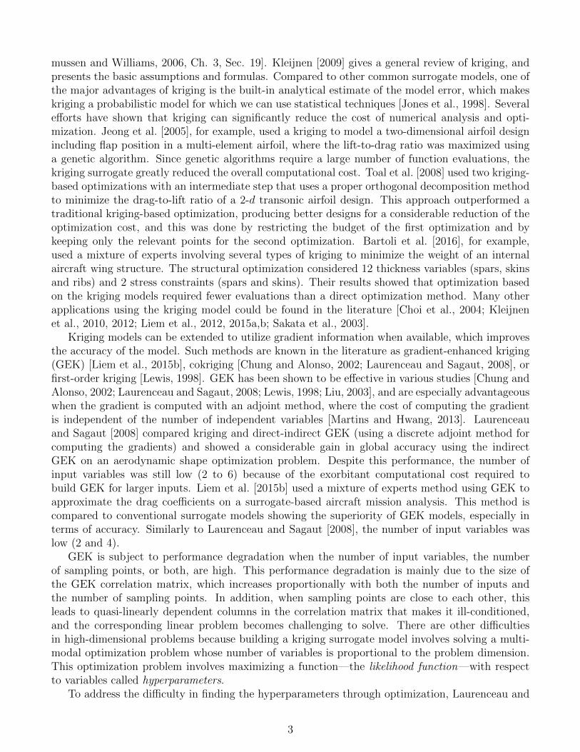
mussen and Williams, 2006, Ch. 3, Sec. 19]. Kleijnen [2009] gives a general review of kriging, andpresents the basic assumptions and formulas. Compared to other common surrogate models, one ofthe major advantages of kriging is the built-in analytical estimate of the model error, which makeskriging a probabilistic model for which we can use statistical techniques [Jones et al., 1998]. Severalefforts have shown that kriging can significantly reduce the cost of numerical analysis and opti-mization. Jeong et al. [2005], for example, used a kriging to model a two-dimensional airfoil designincluding flap position in a multi-element airfoil, where the lift-to-drag ratio was maximized usinga genetic algorithm. Since genetic algorithms require a large number of function evaluations, thekriging surrogate greatly reduced the overall computational cost. Toal et al. [2008] used two kriging-based optimizations with an intermediate step that uses a proper orthogonal decomposition methodto minimize the drag-to-lift ratio of a 2-d transonic airfoil design. This approach outperformed atraditional kriging-based optimization, producing better designs for a considerable reduction of theoptimization cost, and this was done by restricting the budget of the first optimization and bykeeping only the relevant points for the second optimization. Bartoli et al. [2016], for example,used a mixture of experts involving several types of kriging to minimize the weight of an internalaircraft wing structure. The structural optimization considered 12 thickness variables (spars, skinsand ribs) and 2 stress constraints (spars and skins). Their results showed that optimization basedon the kriging models required fewer evaluations than a direct optimization method. Many otherapplications using the kriging model could be found in the literature [Choi et al., 2004; Kleijnenet al., 2010, 2012; Liem et al., 2012, 2015a,b; Sakata et al., 2003].
Kriging models can be extended to utilize gradient information when available, which improvesthe accuracy of the model. Such methods are known in the literature as gradient-enhanced kriging(GEK) [Liem et al., 2015b], cokriging [Chung and Alonso, 2002; Laurenceau and Sagaut, 2008], orfirst-order kriging [Lewis, 1998]. GEK has been shown to be effective in various studies [Chung andAlonso, 2002; Laurenceau and Sagaut, 2008; Lewis, 1998; Liu, 2003], and are especially advantageouswhen the gradient is computed with an adjoint method, where the cost of computing the gradientis independent of the number of independent variables [Martins and Hwang, 2013]. Laurenceauand Sagaut [2008] compared kriging and direct-indirect GEK (using a discrete adjoint method forcomputing the gradients) and showed a considerable gain in global accuracy using the indirectGEK on an aerodynamic shape optimization problem. Despite this performance, the number ofinput variables was still low (2 to 6) because of the exorbitant computational cost required tobuild GEK for larger inputs. Liem et al. [2015b] used a mixture of experts method using GEK toapproximate the drag coefficients on a surrogate-based aircraft mission analysis. This method iscompared to conventional surrogate models showing the superiority of GEK models, especially interms of accuracy. Similarly to Laurenceau and Sagaut [2008], the number of input variables waslow (2 and 4).
GEK is subject to performance degradation when the number of input variables, the numberof sampling points, or both, are high. This performance degradation is mainly due to the size ofthe GEK correlation matrix, which increases proportionally with both the number of inputs andthe number of sampling points. In addition, when sampling points are close to each other, thisleads to quasi-linearly dependent columns in the correlation matrix that makes it ill-conditioned,and the corresponding linear problem becomes challenging to solve. There are other difficultiesin high-dimensional problems because building a kriging surrogate model involves solving a multi-modal optimization problem whose number of variables is proportional to the problem dimension.This optimization problem involves maximizing a function—the likelihood function—with respectto variables called hyperparameters.
To address the difficulty in finding the hyperparameters through optimization, Laurenceau and
3
Sagaut [2008] developed a method that guesses an initial solution of the GEK hyperparameters,and then uses a gradient-based optimization method to maximize the likelihood function. Thismethod accelerates the construction of the GEK model; however, the initial guess depends ona fixed parameter that defines the strength of the correlation between the two most directional-distant sample points. This fixed parameter depends on the physical function to be studied andthus requires trial and error. Therefore, it is not easy to generalize this approach. Lewis [1998] alsotried to accelerate the estimation of the GEK hyperparameters by reducing their number to onefor all directions. The GEK model has shown better results than conventional kriging (using onehyperparameter for all directions) on a borehole flow-rate problem using 8 input variables. However,they assumed that the problem is isotropic, which is not the case for the engineering problems wewant to tackle.
Bouhlel et al. [2016b] proposed an approach that consists in combining the kriging model withthe partial-least squares (PLS) method, called KPLS, to accelerate the kriging construction. Thismethod reduces the number of the kriging hyperparameters by introducing new kernels based on theinformation extracted from the PLS technique. The number of hyperparameters is then reduced tothe number of principal components retained. Experience shows that 2 or 3 principal componentsare usually sufficient to get good accuracy [Bouhlel et al., 2016b]. There is currently no rule ofthumb for the maximum number of principal components to be retained because it depends of boththe problem and location of the sampling points used to fit the model. The KPLS model has shownto be efficient for several high-dimensional problems. Bouhlel et al. [2016b] compared the accuracybetween KPLS and conventional kriging models on analytical and engineering problems problemswith a number of inputs up to 100. Despite the reduced number of hyperparameters used into theKPLS model, they obtained similar results in terms of accuracy between both models. The mainbenefit of KPLS was a reduction in the computational time needed to construct the model: KPSLwas up to 450 faster than conventional kriging.
Another variant of KPLS, called KPLSK, was also developed by Bouhlel et al. [2016a] thatextends the KPLS method by adding a new step into the construction of the model. Once theKPLS method is built, the hyperparameters’ solution is considered as a first guess for a gradient-based optimization applied on a conventional kriging model. The idea of the KPLSK method issimilar to that developed by Ollar et al. [2016], where a gradient-free optimization algorithm is usedwith an isotropic kriging model followed by a gradient-based optimization starting from the solutionprovided by the first optimization. The results of KPLSK have shown a significant improvement onanalytical and engineering problems with up to 60 dimensions in terms of accuracy when comparedto the results of KPLS and conventional kriging. In addition, the KPLSK model is more efficientthan kriging (up to 131 faster using 300 points for a 60D analytical function), and, however, isslightly less efficient than KPLS (22 s vs 0.86 s, respectively, for KPLSK and KPLS with the sametest case). An optimization applications using KPLS and KPLSK could be found in the literature[Bartoli et al., 2016; Bouhlel et al., 2017].
To further improve the efficiency of KPLS and extend GEK to high-dimensional problems, wepropose to integrate the gradient during the construction of KPLS and a different way to use thePLS method. This approach is based on the first order Taylor approximation (FOTA) at eachsampling point. Using this approximation, we generate a set of points around each sampling pointand apply the PLS method for each of these sets. We then combine the information from eachset of points to build a kriging model. We call this new model GE-KPLS since such constructionuses both the gradient information and the PLS method. The GE-KPLS method utilizes gradientinformation and controls the size of the correlation matrix by adding some of the approximatingpoints in the correlation matrix with respect to relevant directions given by the PLS method at
4

each sampling point. The number of hyperparameters to be estimated remains equal to the numberof principal components.
The remainder of the paper is organized as follows. First, we review the key equations forthe kriging and KPLS models in Sections 2.1 and 2.2, respectively. Then, we summarize the twoGEK approaches that already appeared in the literature in Sections 3.1 and 3.2, followed by thedevelopment of the GE-KPLS approach Section 3.3. We then compare the proposed GE-KPLSapproach to the previously developed methods on analytic and engineering cases in Section 4.Finally, we summarize our conclusions in Section 6 after presenting limitations of our approach inSection 5.
2 Kriging surrogate modeling
In this section we introduce the notation and briefly describe the theory behind kriging and KPLS.The first step in the construction of surrogate models is the selection of sample points x(i) ∈ Rd,for i = 1, . . . , n, where d is the number of inputs and n is the number of sampling points. We candenote this set of sample points as a matrix,
X =[x(1)T , . . . ,x(n)T
]T. (1)
Then, the function to be modeled is evaluated at each sample point. We assume that the function tobe modeled is deterministic, and we write it as f : B −→ R, where, for simplicity, B is a hypercubeexpressed by the product between the intervals of each direction space. We obtain the outputs
y =[y(1), . . . , y(n)
]Tby evaluating the function
y(i) = f(x(i)), for i = 1, . . . , n. (2)
With the choice and evaluation of sample points we have (X,y), which we can now use to constructthe surrogate model.
2.1 Conventional kriging
Matheron [1963] developed the theoretical basis of the kriging approach based on the work of Krige[1951]. The kriging approach has since been then extended to the fields of computer simula-tion [Sacks et al., 1989a,b] and machine learning [Welch et al., 1992]. The kriging model, alsoknown as Gaussian process regression [Rasmussen and Williams, 2006], is essentially an interpola-tion method. The interpolated values are modeled by a Gaussian process with mean µ(.) governedby a prior spatial covariance function k(., .). The covariance function k can be written as
k(x,x′) = σ2r(x,x′) = σ2rxx′ , ∀x,x′ ∈ B, (3)
where σ2 is the process variance and rxx′ is the spatial correlation function between x and x′. Thecorrelation function r depends on hyperparameters θ, which need be estimated. In this paper, weuse the Gaussian exponential correlation function for all the numerical results presented in Section 4.
rxx′ =d∏
i=1
exp(−θi (xi − x′i)2
), ∀θi ∈ R+, ∀x,x′ ∈ B, (4)
5

Through this definition, the correlation between two points is related to the distance between thecorresponding points x and x′ This is a function that quantifies resemblance degree between anytwo points in the design space.
Let us now define the stochastic process Y (x) = µ + Z(x), where µ is an unknown constant,and Z(x) is a realization of a stochastic Gaussian process with Z ∼ N (0, σ2). In this study, weuse the ordinary kriging model, where µ(x) = µ = constant. To construct the kriging model, weneed to estimate a set of unknown parameters: θ, µ, and σ2. To this end, we use the maximumlikelihood estimation method. In practice, we use the natural logarithm to simplify the likelihoodmaximization
− 1
2
[n ln(2πσ2) + ln(det R) + (y − 1µ)tR−1(y − 1µ)/σ2
], (5)
where 1 denotes an n-vector of ones.First, we assume that the hyperparameters θ are known, so µ and σ2 are given by
µ =(1TR−11
)−11TR−1y, (6)
where R = [rx(1)X, . . . , rx(n)X] is the correlation matrix with rxX = [rxx(1) , . . . , rxx(n) ]T and
σ2 =1
n(y − 1µ)T R−1 (y − 1µ) . (7)
In fact, Equations (6) and (7) are given by taking derivatives of the likelihood function and settingto zero. Next, we insert both equations into the expression (5) and remove the constant terms, sothe so-called concentrated likelihood function that depends only on θ is given by
− 1
2
[n ln(σ2(θ)) + ln(det R(θ))
], (8)
where σ(θ) and R(θ) denote the dependency with θ. A detailed derivation of these equations isprovided by Forrester et al. [2008] and Kleijnen [2015]. Finally, the best linear unbiased predictor,given the outputs y, is
y(x) = µ+ rTxXR−1 (y − 1µ) , ∀x ∈ B. (9)
Since there is no analytical solution for estimating the hyperparameters θ, it is necessary touse numerical optimization to find the hyperparameters θ that maximize the likelihood function.This step is the most challenging in the construction of the kriging model. This is because, aspreviously mentioned, this estimation involves maximizing the likelihood function, which is oftenmultimodal [Mardia and Watkins, 1989]. Maximizing this function becomes prohibitive for high-dimensional problems (d > 10) due to the cost of computing the determinant of the correlationmatrix and the high number of evaluation needed for optimizing a high-dimensional multimodalproblem. This is the main motivation for the development of the KPLS approach, which we describenext.
2.2 KPLS(K)—Accelerating kriging construction with partial-least squaresregression
As previously mentioned, the estimation of the kriging hyperparameters can be time consuming,particularly for high-dimensional problems. Bouhlel et al. [2016b] recently developed an approachthat reduces the computational cost while maintaining accuracy by using the PLS regression during
6

the hyperparameters estimation process. PLS regression is a well-known method for handling high-dimensional problems, and consists in maximizing the variance between input and output variablesin a smaller subspace, formed by principal components—or latent variables. PLS finds a linearregression model by projecting the predicted variables and the observable variables to a new space.The elements of the principal direction, that is a vector defining the direction of the associatedprincipal component, represent the influence of each input on the output. On the other hand, thehyperparameters θ represent the range in any direction of the space. Assuming, for instance, thatcertain values are less significant in the ith direction, the corresponding θi should have a small value.Thus, the key idea behind the construction of the KPLS model is the use of PLS information toadjust hyperparameters of the kriging model.
We compute the first principal component t1 by seeking the direction w(1) that maximizes thesquared covariance between t1 = Xw(1) and y, i.e.,
w(1) =
{arg max
wwTXTyyTXw
such that wTw = 1.(10)
Next, we compute the residual matrix from X(0) ← X space and from y(0) ← y using
X(1) = X(0) − t1p(1),
y(1) = y(0) − c1t1,(11)
where p(1) (a 1×d vector) contains the regression coefficients of the local regression of X onto the firstprincipal component t1 (an n× 1 vector), and c1 is the regression coefficient of the local regressionof y onto the first principal component t1. Next, the second principal component—orthogonal tothe first principal component—can be sequentially computed by replacing X(0) by X(1) and y(0) byy(1) to solve the maximization problem (10). The same approach is used to iteratively compute theother principal components.
The computed principal components represent the new coordinate system obtained upon ro-tating the original system with axes, x1, . . . , xd [Alberto and Gonzalez, 2012]. The lth principalcomponent tl is
tl = X(l−1)w(l) = Xw(l)∗ , for l = 1, . . . , h. (12)
The matrix W∗ =[w
(1)∗ , . . . , .w
(h)∗
]is obtained by using the following formula [Tenenhaus, 1998,
pg. 114]
W∗ = W(PTW
)−1, (13)
where W =[w(1), . . . ,w(h)
]and P =
[p(1)T , . . . ,p(h)T
]. If h = d, the matrix W∗ =
[w
(1)∗ , . . . ,w
(d)∗
]rotates the coordinate space (x1, . . . , xd) to the new coordinate space (t1, . . . , td), which follows theprincipal directions w(1), . . . ,w(d). More details on the PLS method can be found in the litera-ture [Alberto and Gonzalez, 2012; Frank and Friedman, 1993; Helland, 1988].
The PLS method gives information on any variable contribution to the output. Herein lies theidea developed by Bouhlel et al. [2016b], which consists in using information provided by PLS to
add weights on the hyperparameters θ. For l = 1, . . . , h, the scalars w(l)∗1 , . . . , w
(l)∗d are interpreted as
measuring the importance of x1, . . . , xd, respectively, for constructing the lth principal componentwhere its correlation with the output y is maximized.
To construct the KPLS kernel, we first define the linear map Fl by
Fl :B −→B
x 7−→[w
(l)∗1x1, . . . , w
(l)∗dxd
],
(14)
7
for l = 1, . . . , h. By using the mathematical property that the tensor product of several kernels isa kernel, we build the KPLS kernel
k1:h(x,x′) =h∏
l=1
kl(Fl (x) , Fl (x′)), ∀x,x′ ∈ B, (15)
where kl : B × B → R is an isotropic stationary kernel, which is invariant when translated. Moredetails of this construction are described by Bouhlel et al. [2016b].
If we use the Gaussian correlation function (4) and in this construction (15), we obtain
k(x,x′) = σ2
h∏l=1
d∏i=1
exp
[−θl
(w
(l)∗i xi − w
(l)∗i x′i
)2],∀ θl ∈ [0,+∞[, ∀x,x′ ∈ B. (16)
The KPLS method reduces the number of hyperparameters to be estimated from d to h, whereh << d, thus drastically decreasing the time to construct the model.
[Bouhlel et al., 2016a] proposed another method to construct a KPLS-based model for high-dimensional problems, the so-called KPLSK. This method is applicable only when covariance func-tions used by KPLS are of the exponential type (e.g., all Gaussian), then the covariance functionused by KPLSK is exponential with the same form as the KPLS covariance. This method is basi-cally a two-step approach for optimizing the hyperparameters. The first step consists in optimizingthe hyperparameters of a KPLS covariance, this is by using a gradient-free method on h hyperpa-rameters for a global optimization in the reduced space. The second step consists in optimizing thehyperparameters of a conventional kriging model by using a gradient-based method and the solutionof the first step, this is for a local improvement of the solution provided by the first step into theoriginal space (d hyperparameters). The idea of this approach is to use a gradient-based method,which is more efficient than a gradient-free method, with an initial guess for the construction of aconventional kriging model.
The solution of the first step with h hyperparameters is expressed in the bigger space with dhyperparameters using a change of variables. By using Equation (16) and the change of variable
ηi =h∑
l=1
θlw(l)∗i
2, we get
σ2h∏
l=1
d∏i=1
exp(−θlw(l)
∗i2(xi − x′i)2
)= σ2 exp
(d∑
i=1
h∑l=1
−θlw(l)∗i
2(xi − x′i)2
)= σ2 exp
(d∑
i=1
−ηi(xi − x′i)2)
= σ2d∏
i=1
exp (−ηi(xi − x′i)2) .
(17)
This is the definition of a Gaussian kernel given by Equation (4). Therefore, each component of thestarting point for the gradient-based optimization uses a linear combination of the hyperparameters’solutions from the reduced space. This allows the use of an initial line search along a hypercubeof the original space in order to find a relevant starting point. Furthermore, the final value of thelikelihood function (KPLSK) is improved compared to the one provided by KPLS. The KPLSKmodel is computationally more efficient than a kriging model and slightly more costly than KPLS.
8

3 Gradient-enhanced kriging
If the gradient of the output function at the sampling points is available, we can use this informationto increase the accuracy of the surrogate model. Since a gradient consists of d derivatives, addingthis much information to the function value at each sampling point has the potential to enrichthe model immensely. Furthermore, when the gradient is computed using an adjoint method,whose computational cost is similar that of a single function evaluation and independent of d, thisenrichment can be obtained at much lower computational cost than evaluating d new functionvalues.
Various approaches have been developed for GEK, and two main formulations exist: indirectand direct GEK. In the following, we start with a brief review of these formulations, and then wepresent GE-KPLS—our novel approach.
3.1 Indirect gradient-enhanced kriging
The indirect GEK method consists in using the gradient information to generate new points aroundthe sampling points via linear extrapolation. In each direction of each sampling point, we add onepoint by computing the FOTA
y(x(i) + ∆xje
(j))
= y(x(i))
+∂y(x(i))
∂xj∆xj, (18)
where i = 1, . . . , n, j = 1, . . . , d, ∆xj is the step added in the jth direction, and e(j) is the jth rowof the d × d identity matrix. The indirect GEK method does not require a modification of thekriging code. However, the resulting correlation matrix can rapidly become ill-conditioned, sincethe columns of the matrix due to the FOTA are almost collinear. Moreover, this method increasesthe size of the correlation matrix from n× n to n(d+ 1)× n(d+ 1). Thus, the computational costto build the model becomes prohibitive for high-dimensional problems.
3.2 Direct gradient-enhanced kriging
In the direct GEK method, derivative values are included in the vector y from Equation (9). Thisvector is now
y =[y(x(1)), . . . , y
(x(n)
),∂y(x(1))
∂x1, . . . ,
∂y(x(1))∂xd
, . . . ,∂y(x(n))
∂xd
]T, (19)
with a size of n(d+ 1)× 1. The vector of ones from Equation (9) also has the same size and is
1 = [
n︷ ︸︸ ︷1, . . . , 1,
nd︷ ︸︸ ︷0, . . . , 0]T . (20)
The size of the correlation matrix increases to n(d+ 1)×n(d+ 1), and contains four blocks thatinclude the correlation between the data and themselves, between the gradients and themselves,between the data and gradients, and between the gradients and data. Denoting the GEK correlation
9

matrix by.
R, we can write
.
R=
rx(1)x(1) . . . rx(1)x(n)
∂rx(1)x(1)
∂x(1) . . .∂r
x(1)x(n)
∂x(n)
.... . .
......
. . ....
rx(n)x(1) . . . rx(n)x(n)
∂rx(n)x(1)
∂x(1) . . .∂r
x(n)x(n)
∂x(n)
∂rx(1)x(1)
∂x(1)
T. . .
∂rx(1)x(n)
∂x(1)
T ∂2rx(1)x(1)
∂2x(1) . . .∂2r
x(1)x(n)
∂x(1)∂x(n)
.... . .
......
. . ....
∂rx(n)x(1)
∂x(n)
T. . .
∂rx(n)x(n)
∂x(n)
T ∂2rx(n)x(1)
∂x(n)∂x(1) . . .∂2r
x(n)x(n)
∂2x(n)
, (21)
where, for i, j = 1, . . . , n, ∂rx(i)x(j)/∂x(i), ∂rx(i)x(j)/∂x(j) and ∂2rx(i)x(j)/∂x(i)∂x(j) are given by
∂rx(i)x(j)
∂x(i)=[∂r
x(i)x(j)
∂x(i)k
= −2θk
(x(i)k − x
(j)k
)rx(i)x(j)
]k=1,...,d
, (22)
∂rx(i)x(j)
∂x(j)=[∂r
x(i)x(j)
∂x(j)k
= 2θk
(x(i)k − x
(j)k
)rx(i)x(j)
]k=1,...,d
, (23)
∂2rx(i)x(j)
∂x(i)∂x(j)=[∂2r
x(i)x(j)
∂x(i)k ∂x
(j)l
= −4θkθl
(x(i)k − x
(j)k
)(x(i)l − x
(j)l
)rx(i)x(j)
]k,l=1,...,d
. (24)
Once the hyperparameters θ are estimated, the GEK predictor for any untried x is given by
y(x) = µ+.rTxX
.
R−1
(y − 1µ) , ∀x ∈ B, (25)
where the correlation vector contains correlation values of an untried point x to each training pointfrom X =
[x(1), . . . ,x(n)
]and is
.rxX=
[rxx(1) . . . rxx(n)
∂rx(1)x
∂x(1) . . .∂r
x(n)x
∂x(n)
]T. (26)
Unfortunately, the correlation matrix.
R is dense, and its size increases quadratically both withthe number of variables d and the number of samples n. In addition,
.
R is not symmetric, whichmakes it more costly to invert. In the next section, we develop a new approach that uses thegradient information with a controlled increase in the size of the correlation matrix
.
R.
3.3 GE-KPLS—Gradient-enhanced kriging with partial-least squaresmethod
While effective in several problems, GEK methods are still vulnerable to a number of weaknesses. Aspreviously discussed, the weaknesses have to do with the rapid growth in the size of the correlationmatrix when the number of sampling points, the number of inputs, or both, become large. Moreover,high-dimensional problems lead to a high number of hyperparameters to be estimated, and thisresults in challenging problems in the maximization of the likelihood function. To address theseissues, we propose the GE-KPLS approach, which exploits the gradient information with a slightincrease of the size of the correlation matrix but reduces the number of hyperparameters.
10

3.3.1 Model construction
The key idea of the proposed method consists in using the PLS method around each samplingpoint; we apply the PLS method several times, each time on a different sampling point. To thisend, we use the FOTA (18), to generate a set of points around each sampling point. These newapproximated points are constructed either by a Box–Behnken design [Box et al., 2005, Ch. 11, Sec.6] when d ≥ 3 (Figure 1a) or by a forward and backward variations in the 2d-space (Figure 1b).
(a) Box–Behnken design. (b) Forward and back-ward variations of eachdirection.
Figure 1: The circular and rectangular points are the new generated points and sampling points, respec-tively.
PLS is applied to GEK as follows. Suppose we have a sets of points S = {Si, ∀i = 1, . . . , n},where each set of points is defined by the sampling point
(x(i), y(i)
)and the set of approximating
points generated by FOTA on the Box–Behnken design when d ≥ 3, or on forward and backwardvariations in the 2d-space. We then apply the PLS method on each set of points Si to get the
local influence of each direction space. Next, we compute the mean of the n coefficients∣∣∣w(l)∗
∣∣∣ for
each principal component l = 1, . . . , h. Denoting these new coefficients by w(l)av , we replace the
Equation (14) byFl :B −→B
x 7−→[w(l)
av1x1, . . . , w
(l)avdxd].
(27)
Finally, we follow the same construction used for the KPLS model by substituting w(l)∗ by w
(l)av .
Thus Equation (16) becomes
k(x,x′) = σ2
h∏l=1
d∏i=1
exp[−θl
(w(l)
avixi − w(l)
avix′i)2]
, ∀ θl ∈ [0,+∞[, ∀x,x′ ∈ B. (28)
In the next section, we describe how we control the size of the correlation matrix to obtain thebest trade-off between the accuracy of the model and the computational time.
3.3.2 Controlling the size of the correlation matrix
We have seen in Section 3.1 that the construction of the indirect GEK model consists in adding dpoints around each sampling points. Since the size of the correlation matrix is n(d+1)×n(d+1), thisleads to a dramatic increase in the matrix size. In addition, the added sampling points are close to
11

each other, leading to an ill-conditioned correlation matrix. Thus, the inversion of the correlationmatrix becomes difficult and computationally prohibitive for large numbers of sampling points.However, adding only relevant points improves both the correlation matrix condition number andthe accuracy of the model.
In the previous section, we locally apply the PLS technique with respect to each sampling point,which provides the influence of each input variable around that point. The idea here is to add onlym approximating points (m ∈ [1, d]) around each sampling point, where m is the correspondedhighest coefficients of PLS. To this end, we consider only coefficients given by the first principalcomponent, which usually contains the most useful information. Using this construction, we improvethe accuracy of the model with respect to relevant directions and increase the size of the correlationmatrix to only n(m+ 1)× n(m+ 1), where m << d.
Algorithm 1 describes how the information flows through the construction of the GE-KPLSmodel from sampling data to the final predictor. Once the training points with the associatedderivatives, the number of principal components and the number of extra points are initialized, wecompute w
(1)av , . . . ,w
(h)av . To this end, we construct Si, apply the PLS on Si, and select the mth
most influential Cartesian directions from the first principal component, this is for each samplepoint. Then, we maximize the concentrated likelihood function given by Equation (8), and finally,we express the prediction y given by Equation (9).
Algorithm 1: Construct GE-KPLS model
input :(X,y, ∂y
∂X, h,m
)output: y(x)for i ≤ n doSi; // To generate a set of approximating points
SiPLS−→
(w
(1)∗ , . . . ,w
(h)∗
)max
∣∣∣w(1)∗
∣∣∣; // To select the mth most influential coefficients
end
w(1)av , . . . ,w
(h)av ; // To compute the average of the PLS coefficients
θ1, . . . , θh; // To estimate the hyperparameters
y(x)
In the GE-KPLS method, the PLS technique is locally applied around each sampling point in-stead of the whole space, as in the KPLS model. This enables us to identify the locally influence ofthe input variables where sampling points are located. By taking the mean of all the local input vari-able influences, we expect to obtain a good estimation of the global input variable influences. Themain computational advantages in such construction are the reduced number of hyperparameters tobe estimated—since h << d—and the reduced size of the correlation matrix—n(m+ 1)×n(m+ 1),with m << d, compared to n(d+1)×n(d+1) for the conventional indirect and direct GEK models.
In the next section, our proposed methods are performed on high-dimensional benchmark func-tions and engineering cases.
4 Numerical experiments
To evaluate the computational cost and accuracy of the proposed GE-KPLS method, we perform aseries of numerical experiments where we compare GE-KPLS to other previously developed models
12

for a number of benchmark functions. The first set of functions consists of two different analyticfunctions of varying dimensionality given by
y1(x) =d∑
i=1
x2i , −10 ≤ xi ≤ 10, for i = 1, . . . , d. (29)
y2(x) = x31 +d∑
i=2
x2i , −10 ≤ xi ≤ 10, for i = 1, . . . , d. (30)
The second set of functions is a series of eight functions corresponding to engineering problemslisted in Table 2.
Table 2: Definition of engineering functions.
Problem d n1 n2 Reference
P1 Welded beam 2 10 20 Deb [1998]P2 Welded beam 2 10 20 Deb [1998]P3 Welded beam 4 20 40 Deb [1998]P4 Borehole 8 16 80 Morris et al. [1993]P5 Robot 8 16 80 An and Owen [2001]P6 Aircraft wing 10 20 100 Forrester et al. [2008]P7 Vibration 15 75 150 Liping et al. [2006]P8 Vibration 15 75 150 Liping et al. [2006]
Since the GEK model does not perform well, especially when the number of sampling pointsis relatively high as discussed previously, we performed three different studies. The first studyconsists in comparing GE-KPLS with the indirect GEK and ordinary kriging models on the twoanalytic functions defined by Equations (29) and (30). The second and third studies, which usethe same analytic functions as the first study and the engineering functions respectively, consistin comparing GE-KPLS with the ordinary kriging, KPLS and KPLSK models with an increasednumber of sampling compared to the first study.
The kriging, GEK, and KPLS(K) models, using the Gaussian kernels (4) and (16), respectively,provide the benchmark results that we compared to the GE-KPLS model, using the Gaussian ker-nel (28). We use an unknown constant, µ, as a trend for all model. For the kriging experiments, weuse the scikit-learn implementation [Pedregosa et al., 2011]. Moreover, the indirect GEK methoddoes not require a modification of the kriging source code, so we use the same scikit-learn imple-mentation.
We vary the number of extra points, m, from 0 to 5 in all cases except for the first study, wherein addition we use m = d, and also for the third study when the number of inputs is less than 5input variables; e.g., P1 from the engineering functions where m = 1 and m = d = 2. To refer to thenumber of extra points, we denote GE-KPLS with m extra points by GE-KPLSm. We ran priortests varying the number of principal components from 1 to 3 for the KPLS and KPLSK models,and 3 principal components always provided the best results. Using more principal componentsthan 3 becomes more costly and results in a very slight difference in terms of accuracy (more orless accurate depending on the problem). For the sake of simplicity, we consider only results with 3principal components for KPLS and KPLSK. Similarly, the GE-KPLS method uses only 1 principalcomponent, which was found to be optimal.
13

Because the GEK and GE-KPLS models use additional information (the gradient components)compared to other models and to make the comparison as fair as possible, the number of samplingpoints n used to construct the GEK and GE-KPLS models is always twice less than the numberof samples used for other models in all test cases. This factor of two is to account for the cost ofcomputing the gradient; when an adjoint method is available, this cost is roughly the same or lessthan the cost of computing the function itself Kenway et al. [2014]; Martins and Hwang [2013].
To generate approximation points with FOTA, Laurenceau and Sagaut [2008] recommend touse a step of 10−4li, where li is the length between the upper and lower bounds in the ith direction.However, we found in our test cases that the best step is not always 10−4li, so we performed ananalysis to compute the best step value for the second and third studies. The computational timeneeded to find the best step is not considered and we only report the computational time needed toconstruct the GE-KPLS models using this best step. Because the GEK model is very expensive insome cases (see Section 4.1), we only use the recommended step by Laurenceau and Sagaut [2008]to perform the GE-KPLS and GEK methods for the first study.
To compare the accuracy of the various surrogate models, we compute the relative error (RE)for nv validation points as follows
RE =‖y − y‖‖y‖
, (31)
where y is the surrogate model values evaluated at validation points, y is the corresponding ref-erence function values, and ‖.‖ is the L2 norm. Since in this paper we use explicit functions, thereference values can be assumed to have a machine epsilon of O (10−16). In addition, the functioncomputations are fast, so generating a large set of random validation points is tractable. We usenv = 5, 000 validation points for all cases. The sampling points and validation points are generatedusing the Latin hypercube implementation in the pyDOE toolbox [Abraham, 2009] using a maximinand random criteria, respectively. We perform 10 trials for each case and we always plot the meanof our results. Finally, all computations are performed on an Intel R© CoreTM i7-6700K 4.00 GHzCPU .
4.1 Numerical results for the analytical functions: first study
To benchmark the performance of our approach, we first use the two analytical functions (29)and (30) and compare GE-KPLSm, for m = 1, . . . , 5 and m = d, to the GEK and kriging models.For this study, we have added the case where m = d (compared to the next two studies) to figureout the usefulness of the PLS method in our approach, since the number of extra points is the sameas for the GEK model. We vary the number of inputs for both functions from d = 20 to d = 100by adding 20 dimensions at a time. In addition, we vary the number of sampling points in all casesfrom n = 10 to n = 100 by adding 10 samples at the time for the GEK and GE-KPLS models. Forthe construction of the kriging model, we use 2n sampling points for each case.
Figure 2 summarizes the results of this first study. The first two columns show the RE for y1and y2, respectively, and the other two columns show the computational time for the same twofunctions. Each row shows the results for increasing dimensionality, starting with d = 20 at the topand ending at d = 100 at the bottom. The models are color coded as shown in the legend on theupper right. In some cases, we could not reach 100 sampling points because of the ill-conditionedcovariance matrix provided by the GEK model, which explains the missed experiments in all casesexcept for the y1 function with d = 40.
14

0.05
0.15
0.25d=20
y1 error
d=20
y2 error
10-1
100
101d=20
y1 time (s)
d=20
y2 time (s)
0.05
0.15
0.25 d=40 d=40
101102103 d=40 d=40
0.05
0.15
0.25 d=60 d=60
101
102
103d=60 d=60
0.05
0.15
0.25 d=80 d=80
101
102
103d=80 d=80
10 30 50 70 90
n
0.05
0.15
0.25 d=100
10 30 50 70 90
n
d=100
10 30 50 70 90
n
101102103104 d=100
10 30 50 70 90
n
d=100
Kriging
GEK
GE-KPLS1
GE-KPLS2
GE-KPLS3
GE-KPLS4
GE-KPLS5
GE-KPLSd
Figure 2: Summary of the mean results for kriging, GEK, and GE-KPLS models applied to the analyticalproblems, based on 10 trials for each case. The models are color coded according to the legend (upperright).
The GE-KPLSd and GEK use the same points (training and approximating points) into theircorrelation matrices, and the difference between both models consists in reducing the number ofhyperparameters by PLS for only the first model, so we can verify the scalability of the GE-KPLSmodel with the inputs variables (through the hyperparameters). The GE-KPLSd model yields amore accurate model compared to GEK in all cases except for y1 when d ≥ 40 and n = 10, and fory2 when d > 40 and n = 10. These results show the effectiveness of the PLS method in reducingthe computational time especially when d > 60. For example, the computational time for the y2function with d = 80 and n ≤ 50 is less than 45 s for PLS compared to the computational time ofGEK where it reaches 42 min. Therefore, the PLS method improves the accuracy of the model andreduces the computational time needed to construct the model.
Even though the RE-convergence of GE-KPLSd is the most accurate, the GE-KPLSm modelsfor m = 1, . . . , 5 are in some cases preferable. For example, the GE-KPLSm models for m = 1, . . . , 5are over 37 times faster than the GE-KPLSd model with about a 1.5% of lost in term of error for y1with d = 100 and n = 70. In addition, including d extra points around each sampling point leadsto ill-conditioned matrices, in particular when the number of sampling points is high. Furthermore,the GE-KPLSm models for m = 1, . . . , 5 always yield a lower RE and decreased computational timecompared to kriging. When comparing kriging and GE-KPLSm for m = 1, . . . , 5, the computational
15

time of GE-KPLSm is 10 s lower for all cases and the RE is 10% better in some cases; e.g. they1 function with d = 20, n = 30 using a GE-KPLS5 model. Compared to GEK, GE-KPLSm form = 1, . . . , 5 has a better RE convergence with the y1 function, and the RE convergence on y2 isslightly better with GEK when d ≤ 80. In addition, GE-KPLSm has lower computational timescompared to GEK; e.g. the time needed to construct GE-KPLSm with m = 1, . . . , 5 for y1 with100d and 70 points is between 7 s and 9 s compared to about 27000 s for GEK.
We also note that the difference between the two functions y1 and y2 is only about the firstterm x1, and despite these similarities, the results for both functions are different. For example, theRE-convergence of all GE-KPLSm are better than the GEK convergence for y1 with d = 40, whichis not the case for y2 with d = 40. Therefore, it is safer to make a new selection of the best modelfor a function even though we know the best model for a similar function to the first one.
Finally, the construction of the GEK model could be prohibitive in terms of computational time.For instance, we need about 7.4 hours to construct a GEK model for y1 with d = 100 and n = 70.Thus, the GEK model is not feasible when the number of sampling points is high.
In the next section, we increase the number of sampling points on the same analytic functionand compare the GE-KPLSm models for m = 1, . . . , 5 to the kriging, KPLS and KPLSK models
4.2 Numerical results for the analytical functions: second study
For the second study, we use again the analytical functions y1 and y2 respectively given by Equa-tions (29) and (29). For each case, the number of sampling points, n, used is equal to kd, withk = 2, 10, for the kriging, KPLS and KPLSK models, while n
2sampling points are used for the
GE-KPLSm models. To analyze the trade-off between the computational time and RE, we plot thecomputational time versus RE in Figure 3, where each line represents a given surrogate model usingtwo different numbers of samples. Each line has two points corresponding to n1 = 2d and n2 = 10dsampling points for the kriging, KPLS, and KPLSK models; and to n1
2and n2
2for the GE-KPLSm
models. The models are color coded according to the legend in the upper right sequence of modelnames, starting with kriging through GE-KPLS5. The rows in this grid show the results of differentfunctions, starting with y1 on the top, and ending with y2 in the bottom. The columns show theresults of different dimensions, starting with d = 10 on the left, and ending with d = 100 dimensionson the right of the corresponding function. More detailed numerical results for the mean of the REand computational time are listed in Table 3 in Appendix B.
16

10-2 10-1 100 101 102
0.05
0.15
0.25
20
100
y1 , d=10
10-1 100 101 102 103
0.01
0.03
0.05
0.07
200
1000
y1 , d=100Kriging n1 n2
KPLS
KPLSK
GE-KPLS1 n1
2
n2
2
GE-KPLS2
GE-KPLS3
GE-KPLS4
GE-KPLS5
10-2 10-1 100 101
0.1
0.2
0.3
0.4
20
100
y2 , d=10
10-1 100 101 102 103
0.02
0.06
0.10 200
1000
y2 , d=100
time (s)
err
or
Figure 3: Summary of results for all models and analytical problems, based on 10 trials for each case. Themodels are color coded as shown legend (upper right). The best trade-off between time and error is alwaysobtained by a GE-KPLS model.
As we can see in Figure 3, adding m extra points to the correlation matrix improves the accuracyof the results, and the best trade-off between time and error is always obtained given by a GE-KPLSmodel. At the expense of a slight increase in computational time, increasing the number of extrapoints always yields to a lower error in almost all cases. Indeed, the GE-KPLS5 yields to a lowererror for all cases except for y1 and y2 with 10 dimensions and 50 sampling points, where the lowesterror is obtained with the GE-KPLS2 and GE-KPLS3 models, respectively. Thus, the number ofextra points must be carefully selected.
We can evaluate the performance by either comparing the computational time required to achievea certain level of accuracy, or by comparing the accuracy for a given computational time. GE-KPLS1, for instance, provides an excellent compromise between error and computational time, asit is able to achieve a RE lower than 1% under 0.1 s for the y1 function with 10 dimensions and 50points. Even better, the GE-KPLS5 yields a lower RE using 100 sampling points than the krigingmodel using 1000 sampling points (1.94% vs. 2.96%) for the y1 function with d = 100. In this case,the computational time required to build a GE-KPLS3 is lower by a factor of 9 compared to thecomputational time needed by kriging (12.4 s vs 109.6 s). In addition, the GE-KPLS method is ableto avoid ill-conditioned correlation matrices by reducing the number of extra points through thePLS approach.
Thus, this second study confirms the efficiency of the GE-KPLSm models and their ability togenerate accurate models.
17

4.3 Numerical results for the engineering functions: third study
We now assess the performance of the GE-KPLS models on 8 engineering functions P1, . . . ,P8 listedin Table 2. The first three functions are the deflection, bending stress, and shear stress of weldedbeam problem [Deb, 1998]. The fourth function considers the water flow rate through a boreholethat is drilled from the ground surface through two aquifers [Morris et al., 1993]. The Fifth functiongives the position of a robot arm [An and Owen, 2001]. The sixth function estimates the weight ofa light aircraft wing [Forrester et al., 2008]. P7 and P8 are, respectively, the weight and the lowestnatural frequency of a torsion vibration problem [Liping et al., 2006]. The number of dimensionsfor each of these problems varies from 2 to 15. The detailed formulation for these problems isprovided in Appendix A. In this study, we have intentionally chosen to cover a large engineeringareas using a different number of dimensions and complexities, thus we can verify the generalizationand the applicability of our approach. To build the kriging, KPLS, and KPLSK models, we use twodifferent number of sampling points, n1 = 2d and n2 = 10d, for all problems except for P1, P2 andP3 where n1 = 5d (see Table 2 for more details). Similarly, we use n1/2 and n2/2 sampling pointsfor the GE-KPLS models. We use GE-KPLS to construct surrogate models for these engineeringfunctions, and compare our results to those obtained by kriging, KPLS, and KPLSK. As in theanalytical cases, we performed 10 trials for each case and used the same metrics of comparison:computational time and RE. For our GE-KPLS surrogate model and as previously mentioned, wevary the number of extra points m with m = 1, . . . , 5 and use one principal component for allproblems, except for P1, P2 and P3 where we use at most 2, 2 and 4 extra points, respectively.
Figure 4 shows the numerical results for the engineering functions. As in the plots for theanalytical cases, each line has two points corresponding to n1 and n2 sampling points for thekriging, KPLS, and KPLSK models; and to n1/2 and n2/2 for the GE-KPLSm models. The modelsare color coded according to the legend on the upper right. This grid of plots shows the results ofdifferent problems, starting from P1 on the top left and ending with P8 on the bottom center. Theactual mean values of computational time and RE are given in the Table 4 in Appendix C.
Overall, the GE-KPLS method yields a more accurate solution except for P2. For the P2
function, GE-KPLS2 is almost as accurate than kriging (the model giving the best result) using10 and 20 sampling points, respectively, with a relative error of 0.1866 for the former and 0.1859for the latter. All of the GE-KPLS results have either a lower computational time, lower error, orboth, when compared to the kriging results for the same sampling cost. This means that despitethe augmented size of the GE-KPLS correlation matrices, the computational time required to buildthese models is lower than the kriging model. The efficiency of GE-KPLS is due to the reducednumber of hyperparameters that need to be estimated, which is 1 in our case, compared to dhyperparameters for kriging. In addition, our strategy of how using the PLS coefficients to rescalethe correlation matrix results in better accuracy. For example, we need only 0.12 s for P5 with 80sampling points to build a GE-KPLS5 model with a relative error of 0.3165 compared to 38.9 s fora kriging model (best error given the benchmark) with a relative error of 0.4050.
In Figure 4, we notice that the computational time required to train some models for P1 and P2
seems higher when decreasing the number of sampling points, like for example the KPLSK modelfor P2. This is due to the fast construction of the model for such problems with low dimensions,and the difference in computational time using the different number of sampling points is less than10−3 s.
This study shows that the GE-KPLS model is accurate and computationally efficient for dif-ferent engineering fields. In addition, a given user is able to choose the best compromise betweencomputational time and error. One way to do it is to start by the construction of a GE-KPLS1
18

10-3 10-2 10-1
0.2
0.3
0.4
0.5
10
20
p1
10-3 10-2 10-1
0.2
0.3
0.4
0.5
10
20
p2
10-2 10-1 100 101
0.06
0.10
0.14
0.18
20
40
p3
10-2 10-1 100
0.02
0.06
0.10
0.14
16
80
p4
10-2 10-1 100 101 102
0.35
0.40
0.45
0.5016
80
p5
10-2 10-1 100 101
0.01
0.03
0.05
20
100
p6
10-2 10-1 100 101
0.002
0.006
0.010
0.014
30
150
p7
10-2 10-1 100 101
0.01
0.02
0.03
30
150
p8
Kriging n1 n2
KPLSKPLSKGE-KPLS1 n1
2
n2
2
GE-KPLS2GE-KPLS3GE-KPLS4GE-KPLS5
time (s)err
or
Figure 4: Summary of results for all models and engineering problems, based on 10 trials for each case.The models are color coded as shown in legend (upper right). The best trade-off (time vs error) is alwaysobtained by a GE-KPLS models.
19

model. Then, the user fixes a reasonable trade-off between the error and the computational time(guided by the first results), and subsequently adds more approximating points to achieve suchcompromise. Another way to select m is to define a threshold and to keep approximating pointswith a higher PLS coefficients. We also note that the selection of the number of additional pointsm should be carefully done by the user with regards to his final goal. For example, if the user usesa surrogate model within an iterative optimization design process, it is better to select a GE-KPLSmodel with a relatively low number of approximating points, since new many sampling points wouldbe added close to each other in a small region that quickly deteriorate the condition number of thecorrelation matrix. In the other side, if the final goal is to construct an accurate surrogate modelover the design space, the number of approximating points m could be relatively high.
5 Limitation of the GE-KPLS method
Despite the numerous advantages of the proposed method relative to established models in theliterature, there are still some issues that the use must be concerned with. The major issue withGE-KPLS, which is a common issue with most methods in the literature, is what values to usein certain model parameters. One of these parameters is the step size of FOTA, that was firstoptimized when GE-KPLS is used in Sections 4.1, 4.2 and 4.3, is an important parameter thatcan influence the final results, as this parameter is very sensitive to the type of problem and thesampling points.
In terms of implementation, the current toolbox version to build GE-KPLS cannot handle prob-lems with a large number of both dimensions and sampling points. This issue is mainly due to thememory required during the inversion of the correlation matrix. An approximation of this memorylimit is given by n = 30550d−0.427. This estimation is fit by an approximation of the tendencybetween n and d through Microsoft Excel.
6 Conclusions
We developed a novel approach that uses gradient information at the sampling points that buildsaccurate kriging surrogate models for high-dimensional problems efficiently. The proposed approachdiffers from classical strategies, such as the indirect and direct gradient enhanced kriging in that weexploit the gradient information without dramatically increasing the size of the correlation matrix,and we reduce the number of hyperparameters. We applied the PLS method on each samplingpoint and selected the most relevant approximating points to include into the correlation matrixgiven by the PLS information. Through some elementary operations on the kernels, we acceleratedthe construction of the model by using the average of all computed PLS information to reduce thenumber of hyperparameters. Thus, our approach scales well the number of independent variablesby reducing the number of hyperparameters, and the number of sampling points by selecting onlyrelevant approximating points.
To demonstrate the computational efficiency and the accuracy of the proposed model, we pre-sented a series of comparisons for both analytic functions and engineering problems with differentnumber of both dimensions and sampling points. Three comparison studies were performed. Wefirst compared our approach using m extra points for m = 1, . . . , 5 and m = d to the indirectgradient enhanced kriging and ordinary kriging models. With m = d, which is the same numberof extra points used for gradient enhanced kriging, we showed the usefulness of the PLS methodin terms of computational time and error. The results of this study also demonstrated the effec-
20

tiveness and accuracy of the GE-KPLSm models for m = 1, . . . , 5 when compared to other models.In some cases, the GE-KPLS model is over 3 times more accurate and over 3200 times faster thanthe indirect GEK model. In the second study, we increased the number of sampling points for thesame analytic functions to compare the GE-KPLSm for m = 1, . . . , 5 with the kriging, KPLS, andKPLSK models. This study confirmed the results obtained by the first study, and GE-KPLS showsexcellent performance both in terms of the computational time and the relative error. For the firstfunction and compared to both kriging and KPLS models, the accuracy is an order of magnitudesmaller. The third study focused on 8 engineering functions using the GE-KPLSm for m = 1, . . . , 5and the kriging and KPLS(K) models. The GE-KPLS models yielded more accurate models for 7problems irrespective of the number of both dimensions and sampling points. The improvement interms of relative error provided by the GE-KPLS model is up to 9% in some cases.
GE-KPLS is able to freely manage the number of approximating points for avoiding ill-conditionedmatrices with an important gain in terms of computational time and accuracy. This kind of flex-ibility is very convenient in real applications especially when the surrogate model is used withinan iterative sampling method; e.g. optimization design. Indeed, the user can reduce progressivelythe number of approximating points after a certain number of iterations for minimizing the risk ofill-conditioned problems, that is not available, or needs more sophisticated techniques, with stan-dard gradient-enhanced kriging. For an effective use of our method, we recommend a prior analysisof the step parameter. Unfortunately, this parameter is a problem dependent and is impossible toguess in advance. Actually, this is a common difficulty for all gradient-based methods. Finally, Alltest functions and models used in this paper are available on https://github.com/SMTorg/SMT,and could be reproduced.
A Definition of the engineering cases
The analytical expressions of engineering cases are given by
A.1 P1, P2 and P3
The three responses are the deflection δ, bending stress σ, and shear stress τ of a welded beamproblem [Deb, 1998], respectively.
P1 : δ =2.1952
t3b,
P2 : σ =504000
t2b,
P3 : τ =
√τ ′2 + τ ′′2 + lτ ′τ ′′√0.25 (l2 + (h+ t)2)
,
where
τ ′ =6000√
2hl, τ ′′ =
6000(14 + 0.5l)√
0.25 (l2 + (h+ t)2)
2[0.707hl
(l2
12+ 0.25(h+ t)2
)]and
21

Input variables Range
h [0.125, 1]b [0.1, 1]l, t [5, 10]
A.2 P4
This problem characterizes the flow of water through a borehole that is drilled from the groundsurface through two aquifers [Morris et al., 1993]. The water flow rate (m3/yr) is given by
P4 : y =2πTu (Hu −Hl)
ln(
rrw
)[1 + 2LTu
ln( rrw
)r2wKw+ Tu
Tl
] ,where
Input variables Range Input variables Range
rw [0.05, 0.15] r [100, 50000]Tu [63070, 115600] Hu [990, 1110]Tl [63.1, 116] Hl [700, 820]L [1120, 1680] Kw [9855, 12045]
A.3 P5
This function represents the position of a robot arm given by [An and Owen, 2001]
P5 : y =
√√√√( 4∑i=1
Li cos
(i∑
j=1
θj
))2
+
(4∑
i=1
Li sin
(i∑
j=1
θj
))2
,
where
Input variables Range
Li [0, 1]θj [0, 2π]
A.4 P6
This consists in an estimate of the weight of a light aircraft wing, given by [Forrester et al., 2008]
P6 : y = 0.036S0.758w W 0.0035
fw
(A
cos2 Λ
)q0.006λ0.04
(100tc
cos Λ
)−0.3(NzWdg)
0.49 + SwWp,
where
22

Input variables Range Input variables Range
Sw [150, 200] Wfw [220, 300]A [6, 10] Λ [−10, 10]q [16, 45] λ [0.5, 1]tc [0.08, 0.18] Nz [2.5, 6]Wdg [1700, 2500] Wp [0.025, 0.08]
A.5 P7 and P8
The two quantities of interest in this problem are the weight and the lowest natural frequency of atorsion vibration problem, given by [Liping et al., 2006]
P7 : y =3∑
i=1
λiπLi
(di2
)2
+2∑
j=1
ρjπTj
(Dj
2
)2
,
P8 : y =
√−b−√b2−4c2
2π,
where
Ki =πGidi32Li
, Mj =ρjπtjDj
4g,
Jj = 0.5MjDj
2,
b = −(K1 +K2
J1+K2 +K3
J2
),
c =K1K2 +K2K3 +K3K1
J1J2,
and
Input variables Range Input variables Range
d1 [1.8, 2.2] L1 [9, 11]G1 [105300000, 128700000] λ1 [0.252, 0.308]d2 [1.638, 2.002] L2 [10.8, 13.2]G2 [5580000, 6820000] λ2 [0.144, 0.176]d3 [2.025, 2.475] L3 [7.2, 8.8]G3 [3510000, 4290000] λ3 [0.09, 0.11]D1 [10.8, 13.2] t1 [2.7, 3.3]ρ1 [0.252, 0.308] D2 [12.6, 15.4]t2 [3.6, 4.4] ρ1 [0.09, 0.11]
23
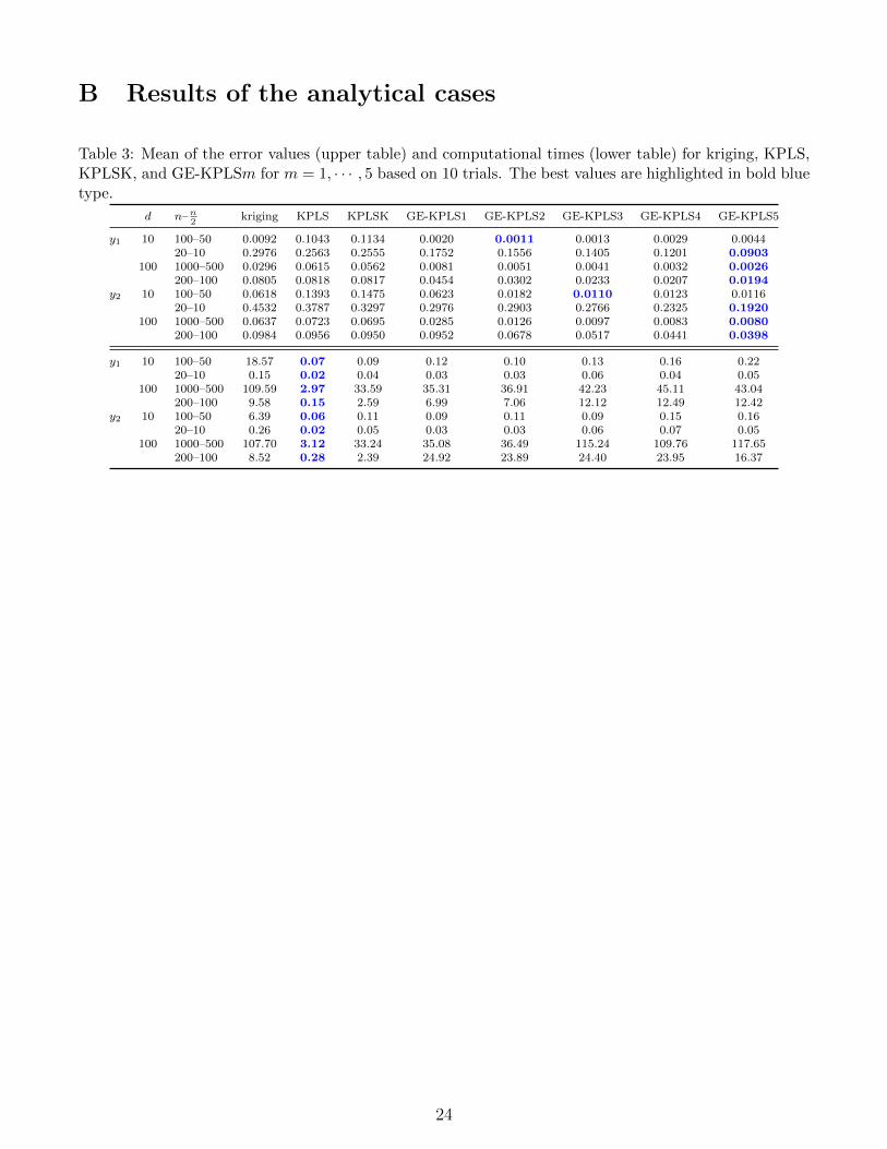
B Results of the analytical cases
Table 3: Mean of the error values (upper table) and computational times (lower table) for kriging, KPLS,KPLSK, and GE-KPLSm for m = 1, · · · , 5 based on 10 trials. The best values are highlighted in bold bluetype.
d n–n2
kriging KPLS KPLSK GE-KPLS1 GE-KPLS2 GE-KPLS3 GE-KPLS4 GE-KPLS5
y1 10 100–50 0.0092 0.1043 0.1134 0.0020 0.0011 0.0013 0.0029 0.004420–10 0.2976 0.2563 0.2555 0.1752 0.1556 0.1405 0.1201 0.0903
100 1000–500 0.0296 0.0615 0.0562 0.0081 0.0051 0.0041 0.0032 0.0026200–100 0.0805 0.0818 0.0817 0.0454 0.0302 0.0233 0.0207 0.0194
y2 10 100–50 0.0618 0.1393 0.1475 0.0623 0.0182 0.0110 0.0123 0.011620–10 0.4532 0.3787 0.3297 0.2976 0.2903 0.2766 0.2325 0.1920
100 1000–500 0.0637 0.0723 0.0695 0.0285 0.0126 0.0097 0.0083 0.0080200–100 0.0984 0.0956 0.0950 0.0952 0.0678 0.0517 0.0441 0.0398
y1 10 100–50 18.57 0.07 0.09 0.12 0.10 0.13 0.16 0.2220–10 0.15 0.02 0.04 0.03 0.03 0.06 0.04 0.05
100 1000–500 109.59 2.97 33.59 35.31 36.91 42.23 45.11 43.04200–100 9.58 0.15 2.59 6.99 7.06 12.12 12.49 12.42
y2 10 100–50 6.39 0.06 0.11 0.09 0.11 0.09 0.15 0.1620–10 0.26 0.02 0.05 0.03 0.03 0.06 0.07 0.05
100 1000–500 107.70 3.12 33.24 35.08 36.49 115.24 109.76 117.65200–100 8.52 0.28 2.39 24.92 23.89 24.40 23.95 16.37
24

C Results of the engineering cases
Table 4: Mean of the error values (upper table) and computational times (lower table) for kriging, KPLS,KPLSK, and GE-KPLSm for m = 1, · · · , 5 based on 10 trials. The best values are highlighted in bold bluetype.
d n–n2
kriging KPLS KPLSK GE-KPLS1 GE-KPLS2 GE-KPLS3 GE-KPLS4 GE-KPLS5
P1 2 20–10 0.1796 0.1881 0.1827 0.2804 0.1791 – – –10–5 0.3747 0.4124 0.4188 0.4639 0.3268 – – –
P2 2 20–10 0.1859 0.2132 0.2216 0.2609 0.1866 – – –10–5 0.3474 0.3478 0.3567 0.4751 0.3904 – – –
P3 4 40–20 0.0607 0.0981 0.0906 0.0940 0.0571 0.0451 0.0692 –20–10 0.1504 0.1933 0.1813 0.1897 0.1132 0.1067 0.1398 –
P4 8 80–40 0.0037 0.0118 0.0091 0.0046 0.0026 0.0019 0.0017 0.007816–8 8.41 0.0999 0.1546 0.0554 0.0325 0.0224 0.0166 0.0151
P5 8 80–40 0.4050 0.4347 0.4296 0.3674 0.3518 0.3376 0.3278 0.316516–8 0.5114 0.4773 0.4707 0.4493 0.4418 0.4405 0.4292 0.4264
P6 10 100–50 0.0023 0.0101 0.0086 0.0085 0.0039 0.0031 0.0022 0.001520–10 0.0260 0.0300 0.0551 0.0225 0.0213 0.0190 0.0158 0.0144
P7 15 150–75 0.0006 0.0008 0.0007 0.0012 0.0008 0.0004 0.0003 0.000230–15 0.0055 0.0072 0.0152 0.0063 0.0034 0.0016 0.0014 0.0011
P8 15 150–75 0.0035 0.0041 0.0037 0.0050 0.0040 0.0029 0.0024 0.002130–15 0.0191 0.0202 0.0308 0.0173 0.0115 0.0085 0.0073 0.0067
P1 2 20–10 0.05 0.006 0.01 0.02 0.01 – – –10–5 0.01 0.006 0.01 0.01 0.01 – – –
P2 2 20–10 0.06 0.006 0.01 0.02 0.01 – – –10–5 0.02 0.006 0.01 0.01 0.01 – – –
P3 4 40–20 1.27 0.01 0.02 0.02 0.03 0.03 0.04 –20–10 0.03 0.01 0.02 0.02 0.02 0.02 0.02 –
P4 8 80–40 0.85 0.03 0.07 0.09 0.07 0.13 0.12 0.1416–8 0.07 0.03 0.04 0.01 0.02 0.02 0.03 0.03
P5 8 80–40 38.90 0.03 0.084 0.07 0.07 0.12 0.10 0.1216–8 0.06 0.03 0.03 0.01 0.02 0.01 0.02 0.02
P6 10 100–50 2.23 0.04 0.10 0.10 0.11 0.11 0.15 0.1720–10 0.09 0.03 0.06 0.02 0.02 0.02 0.018 0.03
P7 15 150–75 4.92 0.05 0.19 0.16 0.16 0.27 0.34 0.3930–15 0.10 0.03 0.05 0.04 0.05 0.27 0.34 0.39
P8 15 150–75 3.01 0.05 0.18 0.12 0.15 0.22 0.27 0.3130–15 0.12 0.03 0.06 0.03 0.04 0.04 0.04 0.04
References
L. Abraham. pydoe: The Experimental Design Package for Python, 2009. URL https:
//pythonhosted.org/pyDOE/index.html. https://pythonhosted.org/pyDOE/index.html.
P. R. Alberto and F. G. Gonzalez. Partial Least Squares Regression on Symmetric Positive-DefiniteMatrices. Revista Colombiana de Estadıstica, 36(1):177–192, 2012.
J. An and A. Owen. Quasi-Regression. Journal of Complexity, 17(4):588–607, 2001.
D. Barber. Bayesian Reasoning and Machine Learning. Cambridge University Press, New York,NY, USA, 2012. ISBN 0521518148, 9780521518147.
N. Bartoli, M. A. Bouhlel, I. Kurek, R. Lafage, T. Lefebvre, J. Morlier, R. Priem, V. Stilz, andR. Regis. Improvement of Efficient Global Optimization with Application to Aircraft wing Design.17th AIAA/ISSMO Multidisciplinary Analysis and Optimization Conference. Washington, D.C.,(AIAA-2016-4001), 2016.
25

M. A. Bouhlel, N. Bartoli, J. Morlier, and A. Otsmane. An Improved Approach for Estimating theHyperparameters of the Kriging Model for High-Dimensional Problems through the Partial LeastSquares Method. Mathematical Problems in Engineering, vol. 2016, Article ID 6723410, 2016a.
M. A. Bouhlel, N. Bartoli, A. Otsmane, and J. Morlier. Improving Kriging Surrogates of High-Dimensional Design Models by Partial Least Squares Dimension Reduction. Structural and Mul-tidisciplinary Optimization, 53(5):935–952, 2016b. ISSN 1615-1488.
M. A. Bouhlel, N. Bartoli, R. G. Regis, A. Otsmane, and J. Morlier. Efficient Global Optimizationfor High-Dimensional Constrained Problems by Using the Kriging Models Combined with thePartial Least Squares Method. Optimization Engineering, 2017.
G. Box, J. Hunter, and W. Hunter. Statistics for experimenters: design, innovation, and discovery.Wiley series in probability and statistics. Wiley-Interscience, 2005. ISBN 9780471718130. URLhttps://books.google.ca/books?id=oYUpAQAAMAAJ.
S. Choi, H. Chung, and J. Alonso. Design of Low-Boom Supersonic Business Jet With Evolu-tionary Algorithms Using Adaptive Unstructured Mesh. 45th AIAA/ASME/ASCE/AHS/ASCStructures, Structural Dynamics and Materials Conference. Palm Springs, California, (AIAA-2004-1758), 2004.
H. S. Chung and J. Alonso. Design of a Low-Boom Supersonic Business Jet Using Cokriging Approx-imation Models. 9th AIAA/ISSMO Symposium on Multidisciplinary Analysis and Optimization,Multidisciplinary Analysis Optimization Conferences, (AIAA-2002-5598), 2002.
N. Cressie. Spatial Prediction and Ordinary Kriging. Mathematical Geology, 20(4):405–421, May1988.
K. Deb. An efficient constraint handling method for genetic algorithms. Computer Methods inApplied Mechanics and Engineering, pages 311–338, 1998.
A. I. J. Forrester, A. Sobester, and A. J. Keane. Engineering Design via Surrogate Modeling: APractical Guide. Wiley, 2008.
I. E. Frank and J. H. Friedman. A Statistical View of Some Chemometrics Regression Tools.Technometrics, 35:109–148, 1993.
R. Haftka, D. Villanueva, and A. Chaudhuri. Parallel surrogate-assisted global optimization withexpensive functions–a survey. Structural and Multidisciplinary Optimization, pages 1–11, 2016.
I. S. Helland. On Structure of Partial Least Squares Regression. Communication in Statistics -Simulation and Computation, 17:581–607, 1988.
S. Jeong, M. Murayama, and K. Yamamoto. Efficient Optimization Design Method Using KrigingModel. Journal of Aircraft, 42(2):413–420, 2005.
D. R. Jones. A taxonomy of global optimization methods based on response surfaces. Journal ofGlobal Optimization, 21(4):345–383, dec 2001.
D. R. Jones, M. Schonlau, and W. J. Welch. Efficient Global Optimization of Expensive Black-BoxFunctions. Journal of Global Optimization, 13(4):455–492, Dec. 1998.
26
G. K. W. Kenway, G. J. Kennedy, and J. R. R. A. Martins. Scalable parallel approach for high-fidelity steady-state aeroelastic analysis and derivative computations. AIAA Journal, 52(5):935–951, May 2014. doi: 10.2514/1.J052255.
J. Kleijnen, W. Van Beers, and I. Van Nieuwenhuyse. Constrained Optimization in ExpensiveSimulation: Novel Approach. European Journal of Operational Research, 202(1):164–174, 2010.
J. Kleijnen, W. Beers, and I. Nieuwenhuyse. Expected Improvement in Efficient Global OptimizationThrough Bootstrapped Kriging. Journal of Global Optimization, 54(1):59–73, 2012.
J. P. C. Kleijnen. Kriging metamodeling in simulation: A review. European Journal of OperationalResearch, 192(3):707–716, 2009. doi: 10.1016/j.ejor.2007.10.013.
J. P. C. Kleijnen. Design and Analysis of Simulation Experiments, volume 230. Springer, 2015.
D. G. Krige. A Statistical Approach to Some Basic Mine Valuation Problems on the Witwatersrand.Journal of the Chemical, Metallurgical and Mining Society, 52:119–139, 1951.
J. Laurenceau and P. Sagaut. Building Efficient Response Surfaces of Aerodynamic Functions withKriging and Cokriging. AIAA Journal, 46:2:498–507, 2008.
R. M. Lewis. Using Sensitivity Information in the Construction of Kriging Models for DesignOptimization. AIAA-98-4799. 7th AIAA/USAF/NASA/ISSMO Symposium on MultidisciplinaryAnalysis and Optimization, Multidisciplinary Analysis Optimization Conferences, pages 730–737,1998.
R. P. Liem, G. K. Kenway, and J. R. R. A. Martins. Multi-point, multi-mission, high-fidelityaerostructural optimization of a long-range aircraft configuration. In Proceedings of the 14thAIAA/ISSMO Multidisciplinary Analysis and Optimization Conference, Indianapolis, IN, Sept.2012. doi: 10.2514/6.2012-5706.
R. P. Liem, K. G. K.W., and J. R. R. A. Martins. Multimission aircraft fuel burn minimizationvia multipoint aerostructural optimization. AIAA Journal, 53(1):104–122, January 2015a. doi:10.2514/1.J052940.
R. P. Liem, C. A. Mader, and J. R. R. A. Martins. Surrogate models and mixtures of experts in aero-dynamic performance prediction for aircraft mission analysis. Aerospace Science and Technology,43:126–151, June 2015b. 10.1016/j.ast.2015.02.019.
W. Liping, B. Don, W. Gene, and R. Mahidhar. A Comparison of Metamodeling Methods Us-ing Practical Industry Requirements. Proceedings of the 47th AIAA/ASME/ASCE/AHS/ASCStructures, Structural Dynamics, and Materials Conference, Newport, RI, 2006.
W. Liu. Development of Gradient-Enhanced Kriging Approximations for Multidisciplinary DesignOptimization. PhD thesis, University of Notre Dame, 2003.
K. V. Mardia and A. J. Watkins. On multimodality of the likelihood in the spatial linear model.Biometrika, 76(2):289, 1989. doi: 10.1093/biomet/76.2.289. URL +http://dx.doi.org/10.
1093/biomet/76.2.289.
27

J. R. R. A. Martins and J. T. Hwang. Review and unification of methods for computing derivativesof multidisciplinary computational models. AIAA Journal, 51(11):2582–2599, November 2013.doi: 10.2514/1.J052184.
G. Matheron. Principles of Geostatistics. Economic Geology, 58(8):1246–1266, 1963.
M. D. Morris, T. J. Mitchell, and D. Ylvisaker. Bayesian Design and Analysis of Computer Exper-iments: Use of Derivatives in Surface Prediction. Technometrics, 35(3):243–255, 1993.
J. Ollar, C. Mortished, R. Jones, J. Sienz, and V. Toropov. Gradient based hyper-parameter opti-misation for well conditioned kriging metamodels. Structural and Multidisciplinary Optimization,pages 1–16, 2016.
F. Pedregosa, G. Varoquaux, A. Gramfort, V. Michel, B. Thirion, O. Grisel, M. Blondel, P. Retten-hofer, R. Weiss, V. Dubourg, J. Vanderplas, A. Passos, D. Cournapeau, M. Brucher, M. Perrot,and E. Duchesnay. Scikit-learn: Machine learning in Python. Journal of Machine LearningResearch, 12:2825–2830, 2011.
C. E. Rasmussen and C. K. I. Williams. Gaussian Processes for Machine Learning. AdaptiveComputation and Machine Learning. MIT Press, Cambridge, MA, USA, Jan. 2006.
J. Sacks, S. B. Schiller, and W. J. Welch. Designs for Computer Experiments. Technometrics, 31(1):41–47, 1989a.
J. Sacks, W. J. Welch, W. J. Mitchell, and H. P. Wynn. Design and Analysis of Computer Experi-ments. Statistical Science, 4(4):409–435, 1989b.
S. Sakata, F. Ashida, and M. Zako. Structural Optimization Using Kriging Approximation. Com-puter Methods in Applied Mechanics and Engineering, 192(417):923–939, 2003.
T. W. Simpson, T. M. Mauery, J. J. Korte, and F. Mistree. Kriging models for global approxima-tion in simulation-based multidisciplinary design optimization. AIAA journal, 39(12):2233–2241,2001a.
T. W. Simpson, J. D. Poplinski, P. N. Koch, and J. K. Allen. Metamodels for computer-basedengineering design: survey and recommendations. Engineering with computers, 17(2):129–150,2001b.
M. Tenenhaus. La Regression PLS: Theorie et Pratique. Ed. Technip, 1998.
D. J. J. Toal, N. W. Bressloff, and A. J. Keane. Geometric filtration using pod for aerodynamicdesign optimization. August 2008. URL http://uos-app00353-si.soton.ac.uk/59225/.
W. J. Welch, R. J. Buck, J. Sacks, H. P. Wynn, T. J. Mitchell, and M. D. Morris. Screening,Predicting, and Computer Experiments. Technometrics, 34(1):15–25, 1992.
28