gps l1 c/a signal acquisition analysis - mitre corporation · gps l1 c/a signal acquisition...

1

GPS L1 C/A Signal Acquisition Analysis

Don Benson

September 21, 2006

Disclaimer

This unclassified document is respectfully submitted for approval for public release. The conclusions, recommendations and results in this report do not necessarily represent those of MITRE or GPSW, but are a working document to be presented and discussed among technical experts before RTCA SC-159 WG-6 (GPS Interference).

Abstract

This report presents a performance analysis of a representative technique for GPS L1 C/A signal acquisition. The purpose of this report is to analyze the signal acquisition technique for L1 C/A legacy aviation GPS receivers to determine C/N0 values where acquisition can occur while satisfying given acquisition scenario constraints. The representative signal acquisition technique is analyzed since receiver manufacturers build to a performance specification and not to a specific acquisition algorithm. The results are based on an acquisition scenario where a position fix must occur within five minuets. Additional conditions for the acquisition are discussed in the report. Results show that acquisition can occur at 28.7 dB-Hz C/N0 at the input to the correlators or 31.7 dB-Hz at the output of the antenna when 1 dB Doppler and code offset losses and 2 dB other implementation losses are included.

Introduction

The purpose of this report is to determine the minimum signal power to noise density ratio, C/N0, that a legacy L1 C/A aviation receiver needs for acquisition of that signal for the scenario described as, “…with latitude and longitude initialized within 60 nautical miles, with time and date within 1 minute, with valid almanac data and unobstructed satellite visibility, … the time from application of power to the first valid position fix shall be less than 5 minutes.” And “Integrity monitoring is provided…” (Reference 1), and with 0.95 confidence (Reference 2). For legacy receivers we assume the probability of missed detection of 0.95 applies to four satellites. We assume 1 minute is allowed to acquire the

mastro

Text Box

Approved for Public Release; Distribution Unlimited Case # 06-1183

2

first SV and ½ minute per SV to acquire the subsequent 3 SVs. Less time is needed for the remaining 3 SVs since the Doppler is determined to one bin from acquiring the first SV. The remaining time is for settling the tracking loops, obtaining and verifying the data (receiving the data message twice), and other overhead functions.

To perform the analysis the following assumptions are also made:

1. 1 ms coherent integration 2. 1 ppm TCXO receiver turn-on oscillator stability results in 6 Doppler bins with 500

Hz bin size for a fixed (zero velocity) location. 3. Code search in ½ chip steps 4. Pfa=0.001, assume total Ptd=0.95 for acquiring 4 SVs 5. Then Pd4 =0.95 and missed detection Pmd=0.01274 for one SV 6. Assumes Pmd is same for all 4 SVs, can be changed or optimized later, where the

optimization is, for example, minimum time to first fix. Analysis of GPS L1 C/A Signal Acquisition

The signal received at the output of the antenna can be written as:

)())cos(()(22))cos(()(12)( 222111 tnttcPttcPts dcadca +++++++= Lφωωφωω (1) We have neglected the additional modulation by the data stream d(t) since we assume that we will not be integrating through a data bit change or if we do, the coherent integration time is small enough (e.g. 1 millisecond) that the effect is negligible. In the above equation: c1, Pa1, ωd1, φ1 is the code, average power at the antenna output, Doppler frequency, and phase of a signal from SV 1, and similarly subscript 2 is for the corresponding signal from SV 2, and so on for other SVs. A more general expression would write the phase due to a

time varying Doppler as: ∫=t

dd dt0 11 )()( ττωφ rather than tt dd 11 )( ωφ = , however we will

assume that the Doppler frequency as constant over short times and treat the phase as piecewise constant over each coherent integration interval. For Pa1 to be average power we must have Pa1 to be the average of the instantaneous power, that is:

∫ +++≅T

dcaa dttttcPT

P0 11

211 ))(2cos1())(1(1 φωω if c1 is normalized so ∫ =

Tdttc

T 0

2 1))(1(1

3

and 0)(2cos))(1(1110

2 ≅++∫ dttttcT d

T

c φωω . This is certainly true for the ideal signal, BPSK-

R, but the normalization must be done for real codes that do not have infinite rise times and do not have discontinuous slopes due to implementation and filtering constraints. ωc is the carrier frequency n(t) is noise in the pass band at the output of the antenna. If we assume the noise is bandlimited we can write the noise, n(t), in terms of its quadrature components as:

ttnttntn dcsdcc )ˆsin()()ˆcos()()( 11 ωωωω +++= (2) Where in Equation 2: nc(t) and ns(t) are the baseband in-phase (I) and quadraphase (Q) components of n(t)

1ˆ dω is the estimate of the Doppler frequency of SV 1. This estimate of Doppler frequency is also in error because of the receiver clock frequency error. In one type of acquisition, estimates of Doppler frequency from Doppler “bins” are used to reduce the signal to in-phase (I) and quadraphase (Q) baseband components as follows. Substitute Equation 2 into Equation 1 and determine two equations by then multiplying by the known quantities tdc )ˆcos( 1ωω + and tdc )ˆsin( 1ωω + , low pass filtering to eliminate the components near 2ωc resulting in:

)()cos()(22)cos()(12)( 22121111 tnttcPttcPtsi ccc +++′++′= Lφδωφδω (3)

)()sin()(22)sin()(12)( 22121111 tnttcPttcPtsq scc +++′++′= Lφδωφδω (4) Where in Equations 3-4 δω11 and δω21 are the Doppler errors and we now use P1c instead of Pa1 where P1c is the power at the correlators. The difference is due to implementation losses such as filtering, A/D conversion, etc. 21 ′′ candc are the code sequence waveforms

resulting from front-end filtering but are normalized so that ∫ =′T

dttcT 0

2 1))(1(1 to preserve

the meaning of average power as discussed earlier. The effect of the front end filtering on signal power loss can be determined from the spectral characteristics of the c1 and the front end filter transfer function. Now multiply Equations 3-4 by the code sequence, c1”(t+ τ) that is offset by the true sequence by an unknown amount, τ, which is to be determined as part of the acquisition. We note here that the receiver generated replica code, c1”, may be and typically is different than both the transmitted code, c1, and the receiver filtered code, c1’. Next perform a coherent integration average for T seconds, where we assume that all the δω are constant over the time, T, to give:

4

∫ +′′+++

++=

T

cc

c

dttctnT

TT

TRP

TT

TRPsic

0212

21

21212

11111

11111

)(1)(1)2/cos(2/

2/sin)(2

)2/cos(2/

2/sin)(2)(

τδωφδωδω

τ

δωφδωδω

ττ

L

(5)

Then for the quadraphase component:

∫ +′′+++

++=

T

sc

c

dttctnT

TT

TRP

TT

TRPsqc

0212

21

21212

11111

11111

)(1)(1)2/sin(2/

2/sin)(2

)2/sin(2/

2/sin)(2)(

τδωφδωδω

τ

δωφδωδω

ττ

L

(6)

5

Where in Equations 5-6: R11(τ) is the cross correlation of the replica code with the filtered signal code for SV 1 and R21(τ) is the cross correlation of the filtered code from SV 2 with the replica code generated for SV 1, that is:

∫ +′′′=T

dttctcT

R0

11 )(1)(11)( ττ (7)

∫ +′′′=T

dttctcT

R0

21 )(1)(21)( ττ (8)

We notice from Equations 5-6 that the replica code spreads the band limited noise terms, nc and ns. We also notice that since both the signal and noise get multiplied by the replica code, normalization of the autocorrelation function of the replica code is not necessary since any multiplicative constant cancels for results that depend on the signal-to-noise ratio. We will,

however, normalize so that for the replica code, ∫ =′′T

dttcT 0

2 1))(1(1 so that we can more

easily quantify the effect of spreading the noise terms by the replica code. We realize that the effect of spreading the noise is analogous to spreading any other signal. That is, we can use the spectral separation methodology to immediately obtain the result. The effects of the spreading on band-limited white noise terms are determined by integrating the power spectral density of the replica code over the minimum bandwidth of either the receiver front end or the bandwidth of the replica code. In general, for any noise, not just band-limited white noise:

∫∫ − ′′

∞

∞− ′′ ΦΦ=ΦΦ=2/

2/ 11 )()()()(β

βdfffNdfffNN cnpnpcnpnpspread (9)

In Equation 9 Nspread is the equivalent noise floor of the noise, Nnp is the noise power, Φnp is the normalized power spectral density (PSD) of the noise power, e.g. ∫

∞

∞−=Φ 1)( dffnp , Φc1”

is the normalized PSD of the replica code, and β is the smaller of the bandwidths of the either the replica code or the receiver front end filtering into the correlators. Coherent integration is performed M times and the result from each coherent integration is non-coherently summed as follows:

∑=

+=M

jjj sqcsicsnc

1

22 )( (10)

This (snc) is the test statistic that determines whether we have acquired the signal or not.

6

This is the optimal test statistic (likelihood ratio) based on the Neyman-Pearson test or a Bayesian hypothesis test. The total time required searching every chip sequentially and every Doppler bin is: Ta=2NcNdTdwell (11) Where: Nc are the number of code chips (1023 for C/A) Nd are the number of Doppler bins. The size of the Doppler bin is usually some fraction of 1/T Hz and the number of bins is determined by dividing the total expected Doppler frequency range by the bin size. The Doppler frequency range can be expressed as (±vmax/c)fc + δfc. vmax is the maximum SV to receiver relative velocity along the line of sight, c is the speed of electromagnetic propagation, and fc is the carrier frequency. δfc is the receiver oscillator error, and we will model this error as: δfc=fc*PPM (12) PPM is the oscillator drift in parts per million. Other terms and models can be used to refine the oscillator error description. Tdwell = M*T (The time spent at each Doppler and code location) (13) The 2 in Equation 11 multiplies the number of code chips since the search is assumed to be performed in half code steps to be sure to have the replica code somewhat correlated with the actual code. In the worst case the replica code would be offset by a quarter of a chip and the correlation function for BPSK-R would by 3/4 instead of 1 for no offset for a rectangular code (infinite bandwidth signal). Note that the actual correlation values would be somewhat different since the filtered code and the replica codes may not be rectangular. The number of integrator pairs (one for I channel and one for Q channel sometimes called complex integrators) required is determined by first dividing the actual sequential search time, Ta, by the required search time, Tr, where Tr is specified as, for example, 60 seconds. A table can now be generated based on hypothesis testing using the probability distribution of Equation 10. We have to pick a probability of false detection, Pfa, and a probability of missed detection, Pmd. If we neglect for now the cross correlation terms, then Equation 10 is chi-square with 2M degrees of freedom when the C/A signal is not present. When the C/A signal is present Equation 10 is non-central chi-square with 2M degrees of freedom and non-centrality parameter:

2

11

1111

0

1

2/)2/sin()(2 ⎟⎟⎠

⎞⎜⎜⎝

⎛=

TTR

NP

MT c

δωδω

τδ (14)

To complete the table, pick an M and determine the threshold based on Pfa and the chi-square distribution. Once the threshold is determined, then determine δ from the non-central chi-square distribution also using M and Pmd. With δ now determined we can use Equation 14 to find P1c/N0 (C/N0 at the input to the correlators) for various assumptions about Doppler error and replica code offset. Also with M known we can determine the number of correlators required to meet the time to first acquisition.

7

For the C/A code cross correlation between two or more codes and the desired code can be important. Cross correlation can be taken into account in the hypothesis test by assuming that when the signal is not present a cross correlation bias can be present. In this case the probability of false alarm or detection, Pfa is non-central Chi-square where the non-centrality parameter depends upon the Doppler differences, the cross correlation functions and the powers of the interfering signals. When the signal is present, the cross correlated signals can add, subtract or contribute anything in between. For this analysis, when the signal is present, we will assume, on the average, the cross correlation adds nothing to the signal power. For the results that were computed, we assume that there is one SV with a large power with no Doppler difference to determine the threshold, and there is no additive effect when the signal is present. This methodology of analyzing the effect of cross correlation was suggested by Van Dierendonck in Reference 3.

Discussion of Results

To compute the results for Figures 1-6, the following assumptions, restated from Section 1, were made:

1. 1 ms coherent integration 2. 1 ppm TCXO receiver oscillator stability results in 6 Doppler bins with 500 Hz bin size for a fixed (zero velocity) location 3. Code search in ½ chip steps 4. Pfa=0.001, assume total Ptd=0.95 for acquiring 4 SVs 5. Then Pd4 =0.95 and missed detection Pmd=0.01274 for one SV 6. Assumes Pmd is same for all 4 SVs, can be changed or optimized later, where the optimization is, for example, minimum time to first fix.

In Figures 1-6, the C/N0 needed at the input to the correlators to acquire the first satellite is plotted as a function of the number of correlator pairs for three different acquisition times and two different power-to-noise density levels causing cross correlation. To determine the required C/N0 at the output of the antenna the Doppler, code, and other implementation losses must be added. Doppler and code offset losses are shown in Table 2 and other implementation losses are typically 2 to 2.5 dB. The treatment of cross correlation for acquisition suggested by Van Dierendonck in Reference 3 is modified in the next sub-section, Acquisition with Constant Power Difference, to account for the fact that as the noise level increases the power-to-noise density of the cross-correlation decreases. The C/A code

8

cross correlation can take on only three values when the delay is an integer number of chips. These are: -1/1023,-65/1023 and 63/1023 and the power-to-noise density ratio is reduced by the square (-60.2,-24.2 and -23.9 dB Reference 4) of these numbers (see Equation 14). If there is Doppler difference between the incoming signal and the replica code there could be a minimum attenuation of only 21.1 dB, however the probability of occurrence for that level of attenuation is small, 0.001, Reference 4. Since it is impossible to determine what the cross correlation will be during signal acquisition and false alarms are undesirable, we use an attenuation of 24.0 dB, thus the power-to-noise density level of 45 dB-Hz would be attenuated by the cross correlation to 21 dB-Hz.

101 10229.5

30

30.5

31

31.5

32

32.5

Number of Correlators

C/N

0 to

Acq

uire

1st

SV

in 1

min

ute

(dB

-Hz)

C/N0 to Acquire 1st SV in 1 Minute With No Doppler and Code Offset Losses

Figure 1. Acquisition C/N0 vs Number of Correlators, 50 dB-Hz Cross-Correlation-1 Minute Required Acquisition Time

9

101 10227

27.5

28

28.5

29

29.5

30

30.5

31


C/N

0 to

Acq

uire

1st

SV

in 1

min

ute

(dB

-Hz)



The acquisition C/N0 of the first SV for 2 and 3 minute acquisition times are shown in Figures 3-6.

10

101 10228.5

29

29.5

30

30.5

31


C/N

0 to

Acq

uire

1st

SV

in 2

min

utes

(dB

-Hz)

C/N0 to Acquire 1st SV in 2 Minutes With No Doppler and Code Offset Losses

Figure 3. Acquisition C/N0 vs Number of Correlators, 50 dB-Hz Cross-Correlation-2 Minutes Required Acquisition Time

11

101 10226

26.5

27

27.5

28

28.5

29

29.5


C/N

0 to

Acq

uire

1st

SV

in 2

min

utes

(dB

-Hz)



12

101 10228

28.5

29

29.5

30

30.5


C/N

0 to

Acq

uire

1st

SV

in 3

min

utes

(dB

-Hz)



13

101 10225.5

26

26.5

27

27.5

28

28.5


C/N

0 to

Acq

uire

1st

SV

in 3

min

utes

(dB

-Hz)



Acquisition with Constant Power Difference

The discussion now will determine the acquisition C/N0 while keeping a constant difference between the acquisition C/N0 and the cross-correlation Ccc/N0. The difference used for the calculations will be based on the difference between the minimum power for the SV to be acquired and the maximum power on the SV for cross-correlation. To clarify again, the discussion of numerical values applies to C/A signals. The minimum power at the output of the receiver antenna is -158.5 dBW -4.5 dB (due to antenna gain at 5° elevation) = -163 dBW (Reference 5). The maximum power is -153 dBW and the product of the L1 user received power profile for IIA, IIR, IIRM and IIF with the receiver antenna gain pattern as a function of elevation angle gives a maximum power at the output of the antenna of -149.2 dbW. This occurs at an elevation angle of 90° giving a difference of 13.8 dB. For the results shown in Figures 1-6, the cross-correlation, Ccc/N0, was fixed at either 45 or 50 dB-Hz and acquisition

14

C/N0 was determined as a function of the number of correlators. Thus the differences between C/N0 and Ccc/N0 are not constant. Using an iterative procedure the computer program can be used to obtain results where the difference is constant. A constant difference is equivalent to finding the maximum noise that can be tolerated to acquire the minimum power SV while the cross-correlation SV is at maximum power as a function of the number of correlators.

From the plots in Figures 7-8 we can determine two points of constant 13.8 dB difference for 1 minute acquisition time for the first SV. From Figure 7 we see that C/N0 of 28.2 dB-Hz is 13.8 dB from the 42 dB-Hz cross-correlation interference. For this value of C/N0 we need 25 integrators. From Figure 8 we see that C/N0 of 29.2 dB-Hz is 13.8 dB from the 43 dB-Hz cross-correlation interference. For this value of C/N0 we need 18 integrators. These two points are in or near the range of the number of integrators we expect in the legacy aviation receivers since the number of integrators is not specified in the receiver requirements.

From the plots in Figures 9-10 we can two points of constant 13.8 dB difference for 2 minute acquisition time for the first SV. From Figure 9 we see that C/N0 of 26.4 dB-Hz is 13.8 dB from the 40.2 dB-Hz cross-correlation interference. For this value of C/N0 we need 25 integrators. From Figure 10 we see that C/N0 of 27.4 dB-Hz is 13.8 dB from the 41.2 dB-Hz cross-correlation interference. For this value of C/N0 we need 18 integrators. A summary of these results is shown in Table 1. We note again that the C/N0 is at the input to the correlators. To determine the C/N0 at the output of the antenna, the Doppler and code offset losses shown in Table 2 must be added as well as the other 2 to 2.5 dB implementation losses.

The legacy receiver is not likely to acquire the first SV at 5° elevation where the power is minimum and there is a large cross-correlation from other SVs. If we assume that the first SV is acquired at 15° or higher elevation then the antenna gain is at least 0 dB. In this case the power difference is 9.3 dB. Results for 18 and 25 integrators are shown in Table 1.

Acquisition of Second through Fourth Satellites

Acquisition of the first SV now reduces the number of Doppler bins from 6 to 1 and the scenario allows 30 seconds each for acquisition of the 2nd through the 4th SV. Figures 11 and 12 show the C/N0 to acquire the 2nd through the 4th SV vs the number of correlators when there is 50 dB-Hz cross-correlation (Figure 11) and when there is 45 dB-Hz cross-correlation (Figure 12). Also included in Table 1 are the results for acquiring the 2nd through the 4th SVs with a constant power difference of 13.8 dB.

For the assumptions made to determine the acquisition, Table 1 shows that acquiring the first SV is the most critical, i.e. has the least amount of margin. Different assumptions could be made that would lead to more balanced acquisition thresholds where the first SV and the others have approximately the same acquisition thresholds.

15

Table 1. Acquisition C/N0 for Constant Power Difference

Time Required to Acquire First SV (13.8 dB Power Difference at 5° elevation)

Acquisition C/N0

dB-Hz

Number of Integrators

29.2 18 1 minute

28.2 25

27.4 18 2 minutes

26.4 25

Time Required to Acquire First SV (9.3 dB Power

Difference at 15° elevation)

28.7 18 1 minute

27.7 25

Time Required to Acquire 2nd through 4th SVs (13.8 dB Power Difference)

26.2 18 ½ minute each

25.3 25

16

101 10226.5

27

27.5

28

28.5

29

29.5

30

30.5

31


C/N

0 to

Acq

uire

1st

SV

in 1

min

ute

(dB

-Hz)



17

101 10226.5

27

27.5

28

28.5

29

29.5

30

30.5

31


C/N

0 to

Acq

uire

1st

SV

in 1

min

ute

(dB

-Hz)



18

101 10225

25.5

26

26.5

27

27.5

28

28.5

29


C/N

0 to

Acq

uire

1st

SV

in 2

min

utes

(dB

-Hz)


Figure 9. Acquisition C/N0 vs Number of Correlators, 40.2 dB-Hz Cross-Correlation-2 Minutes Required Acquisition Time

19

101 10225

25.5

26

26.5

27

27.5

28

28.5

29


C/N

0 to

Acq

uire

1st

SV

in 2

min

utes

(dB

-Hz)


Figure 10. Acquisition C/N0 vs Number of Correlators, 41.2 dB-Hz Cross-Correlation-2 Minutes Required Acquisition Time

20

Performance should improve as the noise is decreased with the threshold fixed. At first this may seem somewhat contradictory since Ccc/N0 will increase but remember that the test statistic is normalized to make unit variance. Performance could improve even further if the threshold was changed as a function of the noise variance, but this requires an adaptive threshold setting that legacy receivers probably have.

101 10228

28.5

29

29.5

30

30.5


C/N

0 to

Acq

uire

2nd

to 4

th S

V in

1/2

min

ute

(dB

-Hz)

C/N0 to Acquire 2nd to 4th SV in 1/2 Minute With No Doppler and Code Offset Losses

Figure 11. Acquisition C/N0 vs Number of Correlators, 50 dB-Hz Cross-Correlation-1/2 Minute Required Acquisition Time, 2nd through 4th SVs

21

101 10225.5

26

26.5

27

27.5

28

28.5


C/N

0 to

Acq

uire

2nd

to 4

th S

V in

1/2

min

ute

(dB

-Hz)

C/N0 to Acquire 2nd to 4th SV in 1/2 Minute With No Doppler and Code Offset Losses

`

Figure 12. Acquisition C/N0 vs Number of Correlators, 45 dB-Hz Cross-Correlation-1/2 Minute Required Acquisition Time, 2nd through 4th SVs

Effect of Code Doppler on Acquisition This paragraph discusses the effect of code Doppler on signal acquisition. The effect of code Doppler on detectable signal power can be determined as follows. For L1 there are 1540 cycles per chip for C/A or 1/1540 chips per cycle. If the code is Doppler shifted for acquisition for the parameters shown at the beginning of this section then the maximum Doppler error is 250 Hz for a 500 Hz Doppler bin. For a 250 Hz maximum Doppler error the code Doppler error would be 250/1540=0.162 chips/sec. For a coherent integration time of 0.001 sec there is a 0.000162 chip error–virtually no signal power degradation. For longer coherent integration times the Doppler bins become narrower. For example, from Table 2 if the coherent integration time is one second the bin size could be 1 Hz and the shifted replica code Doppler error would result in 0.5/1540=0.00032 chip. These conclusions depend upon the assumption that the Doppler frequency is constant (linear phase) during the coherent integration time. Changes in constant Doppler frequency are due to unmodeled SV motion

22

and clock errors and unmodeled receiver motion and clock errors. Ways around this is to add more complexity in the Doppler frequency such as quadratic phase rather than linear phase or non-coherent integration. If the replica code were not Doppler compensated, then the code Doppler error would be 1500/1540=0.974 chips/sec. For a coherent integration time of 0.001 seconds there is a 0.000974 chip error, again virtually no signal power degradation. This error starts to be significant if the coherent integration time is longer than 0.25 seconds. Of possibly more significance is the change in the code bins that the signal can inhabit with respect to the replica code. For the parameters used in this analysis for acquisition and with 50 complex integrators (more than is thought to be in legacy receivers) the dwell time is 0.245 seconds in each cell to acquire the first SV. For this case there are 245 coherent integrations at 0.001 sec per coherent integration. Since the worst case Doppler gives 0.162 chips/sec then 0.245*0.162=0.04 chips. For acquisition of the 2nd through the 4th SVs there are 734 coherent integrations for 50 complex integrators, and this leads to a code advance or delay of 0.12 chips. We can conclude that the effect of code Doppler on acquisition is insignificant. Losses Due to Doppler and Code Offsets

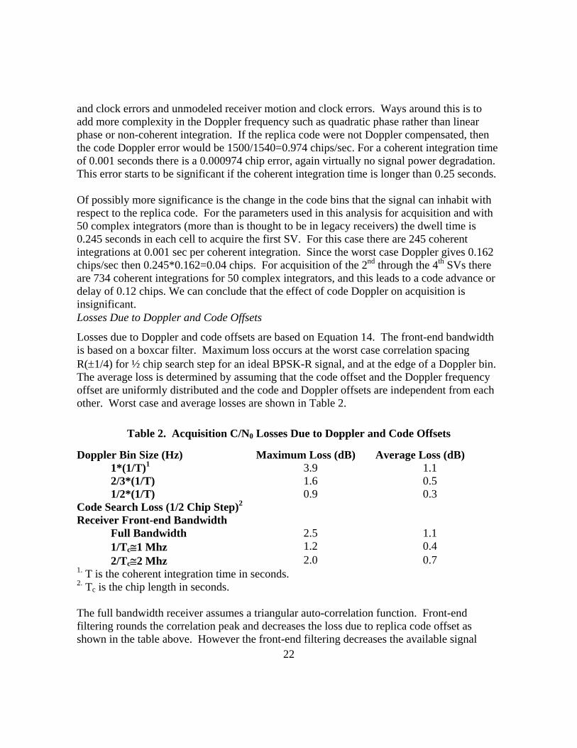
Losses due to Doppler and code offsets are based on Equation 14. The front-end bandwidth is based on a boxcar filter. Maximum loss occurs at the worst case correlation spacing R(±1/4) for ½ chip search step for an ideal BPSK-R signal, and at the edge of a Doppler bin. The average loss is determined by assuming that the code offset and the Doppler frequency offset are uniformly distributed and the code and Doppler offsets are independent from each other. Worst case and average losses are shown in Table 2.

Table 2. Acquisition C/N0 Losses Due to Doppler and Code Offsets

Doppler Bin Size (Hz) Maximum Loss (dB) Average Loss (dB) 1*(1/T)1 3.9 1.1 2/3*(1/T) 1.6 0.5 1/2*(1/T) 0.9 0.3 Code Search Loss (1/2 Chip Step)2 Receiver Front-end Bandwidth

Full Bandwidth 2.5 1.1 1/Tc≅1 Mhz 1.2 0.4 2/Tc≅2 Mhz 2.0 0.7 1. T is the coherent integration time in seconds. 2. Tc is the chip length in seconds. The full bandwidth receiver assumes a triangular auto-correlation function. Front-end filtering rounds the correlation peak and decreases the loss due to replica code offset as shown in the table above. However the front-end filtering decreases the available signal

23

power and this effect is accounted for as part of the implementation loss (usually 2 to 2.5 dB). This implementation loss also includes effects from quantization, signal-in-space imperfections as well as front-end filtering. The motivation for using average losses is well underpinned in hypothesis testing theory (Reference 6). The carrier to noise density ratio can also be considered a random variable if the acquisition strategy of the receiver is to acquire the first SV with the highest elevation (Reference 7). In this case when the signal is present (hypothesis, H1) the conditional probability becomes a probability density for a simple hypothesis test by integrating over the random variables (Reference 6):

(15) The non-centrality parameter given in Equation 14 then becomes:

(16) Average C/N0 was determined approximately for L1 based on modifying L5 results given in Reference 7. The modifications changed the C and N0 for L5 to values appropriate for L1. These results are shown in Figure 13. The antenna profile could not be modified to the L1 profile. New computer runs have to be made to accomplish this. Also the distribution shown in Figure 13 is for the Harrisburg, PA “hot spot”. Other runs should be made for other representative locations over the earth, but the purpose of showing this is to demonstrate the methodology (Reference 8) as well as showing approximately what interference can be tolerated to acquire the first SV.

∫= 010|/,,101|11| /)|/,,(),/,,|()|(10

NdCfddHNCfPHNCfRPHRP HNCfHrHr τδτδτδ τδ

220 })()sin({)(/2 fTfTRNCMT πδπδτδ =

24

Approximate L1 GPS C/N0 Probability Distribution – No Interference

34.9 35.9 36.9 37.9 38.9 39.9 40.9 41.9 42.9C/N0 (dB-Hz)

Approximate L1 GPS C/N0 Probability Distribution – No Interference

34.9 35.9 36.9 37.9 38.9 39.9 40.9 41.9 42.9C/N0 (dB-Hz)

Figure 13. Cumulative Probability Distribution at Receiver Antenna Output

HzdBNC

−= 97.400

25

Steps to Determine Tolerable Interference to Acquire First SV

The results in Table 1 can be used in a number of ways to determine the interference that can be tolerated by the receiver and still achieve the required performance. One way is to compare actual <C/N0> with required <C/N0>. If we interpret the values in Table 1 to mean average C/N0 values then the following steps can be used to determine the additional interference that can be tolerated by the receiver. <•> means average or expected value

1. Comparison must be made at same point, e.g. at output of antenna 2. If actual <C/N0> ≥ <C/N0> required then receiver can acquire with additional

external interference 3. What additional interference can be tolerated? 4. From Table 1 if receiver has required <C/N0> ≅28.7 dB-Hz at input to correlators 5. From Table 2 of average losses 0.3 dB for 500 Hz Doppler bin and 0.7 dB for 2 MHz

front end bandwidth=1.0 dB total search loss 6. Add 2.0 dB implementation loss for quantization, front-end filter and signal-in-space

imperfections gives<C/N0> req=31.7dB-Hz at output of antenna 7. For this case the tolerable interference is determined by solving:

8. IIN

C+

=+

= −

−

15.20

05.16

0

17.3

101010

9. <C> is determined from N0=-201.5dBW/Hz and <C/N0>=40.97 dB-Hz 10. Then from above equation, I=-192.7 dBW/Hz 11. Similarly for a full bandwidth front-end we must solve:

12. IIN

C+

=+

= −

−

15.20

05.16

0

21.3

101010

13. Then from above equation, I=-193.2 dBW/Hz 14. This assumes other implementation loss of 2.0 dB

Conclusions

1. Results show that acquisition can occur at 28.7 dB-Hz C/N0 at the input to the correlators or 31.7 dB-Hz at the output of the antenna when 1 dB Doppler and code offset losses and 2 dB other implementation losses are included. This assumes the legacy receiver has 18 correlators and its search strategy is to acquire the first SV with an elevation angle greater that 15°.

2. If we use the above threshold and assume the legacy receiver’s search strategy is to acquire the highest elevation SV first, then we can determine the additional interference that can be tolerated. The highest elevation SV is assumed to have

26

minimum power of -158.5 dBW at the input to the antenna. The additional interference is -192.7 dBW/Hz for a 2 MHz front end bandwidth.

3. Significant results are summarized in the repeat of Table 1.

Table 3. Acquisition C/N0 for Constant Power Difference (Repeat of Table 1)

Time Required to Acquire First SV (13.8 dB Power Difference at 5° elevation)

Acquisition C/N0

dB-Hz

Number of Integrators

29.2 18 1 minute

28.2 25

27.4 18 2 minutes

26.4 25

Time Required to Acquire First SV (9.3 dB Power

Difference at 15° elevation)

28.7 18 1 minute

27.7 25

Time Required to Acquire 2nd through 4th SVs (13.8 dB Power Difference)

26.2 18 ½ minute each

25.3 25

Recommendations

These recommendations are the result of both knowing items that should be done at the time the report and analysis was being performed but could not be included because of time/manpower constraints, or discovering items that should be done as a result of performing the work.

27

1. Additional performance could be gained with a balanced required C/N0 with the first SV and the remaining SVs, by allowing more time to acquire the first SV and less for the remaining SVs. In this way the total time can be kept constant.

2. A performance analysis should be done for acquiring 5 SVs to insure integrity in the position fix, although acquiring the fifth SV should require negligible time for acquisition and the four SV analysis should be indicative of performance.

3. The antenna gain pattern for L1 should be used when determining the probability distribution for C/N0.

4. Probability distributions for C/N0 similar to that shown in Figure 13 should be determined for various representative locations and times.

5. C/N0 cumulative probability distribution similar to Figure 13 should be determined for a constellation with typical power levels and not minimum power levels. This distribution should then be used for interference levels that can be tolerated.

A more consistent calculation used results that depend on bandwidth could be done. For example we assume that the effect of bandwidth on the signal is lumped in the 2 dB implementation loss but we do an explicit calculation of the effect of front-end bandwidth for code offset losses. We can do an explicit calculation on 1.) the signal loss due to front-end filter 2.) the effect spreading the of front-end bandwidth limited noise by the replica code, and 3.) code offset losses. The implementation loss term, the noise term and the code offset losses would all be a function of bandwidth.

List of References

1. RTCA/DO-229C, Minimum Operational Performance Standards for Global Positioning System/Wide Area Augmentation System Airborne Equipment, November 28, 2001

2. RTCA/DO-208, Minimum Operational Performance Standards forAirborne Supplemental Navigation Equipment Using Global Positioning System (GPS), July 12, 1991

3. Parkinson, B. W. and Spilker, J .J., editors, Global Positioning System: Theroy and Applications Volume 1, Chapter 8, AIAA, 1996, ISBN 1-56347-106-X

4. Kaplan, E.D, and Hegarty, C. J., editors, Understanding GPS, Principles and Applications, 2nd edition, Artech House, 2006, ISBN 1-58053-894-0

5. “Reference Assumptions for GPS/Galileo Compatibility Analysis”, 9 June 2004

6. Van Trees, H., Detection, Estimation, and Modulation Theory, Part 1, Wiley, Inc., 2001, ISBN 0-471-09517-6

28

7. RTCA/DO-292, Assessment of Radio Frequency Interference Relevant to the GNSS L5/E5A Frequency Band, July 29, 2004

8. “A New Methodology for Analysis of GPS Acquisition”, MITRE briefing to RTCA SC 159, WG-6, March 22-23, 2006

gps l1 c/a signal acquisition analysis - mitre corporation · gps l1 c/a signal acquisition...

Documents