GPS-Free Greedy Routing with Delivery Guaranteeand Low Stretch Factor on 2D and 3D Surfaces

Su Xia, Hongyi Wu, and Miao Jin

Abstract—This paper focuses on greedy routing in wirelessnetworks deployed on 2D and 3D surfaces. It introduces adistributed embedding scheme based on the conformal maptheory. The proposed scheme identifies the convex hull of eachboundary and employs Yamabe flow to compute flat metric underconvex hull boundary condition to establish virtual coordinates.Such virtual coordinates are then used for greedy routing. Sincethe proposed embedding algorithm maps the outer boundary to aconvex shape and an interior concave void to a circle-like convexpolygon, it effectively eliminates local minimum and attainsguaranteed delivery. At the same time, it introduces a smalldistortion only and consequently achieves a low stretch factor.Our simulations show that its stretch factor is lower than anyexisting greedy embedding algorithms. Moreover, the proposedscheme is merely based on local connectivity and consumes asmall constant storage, thus scaling to arbitrarily large networks.

I. INTRODUCTION

With both storage space and computation complexitybounded by a small constant, greedy routing is deemed anappealing approach for resource-constrained networks [1]. Inmost cases, a node under greedy routing only needs to storeits coordinates and perform a standard distance calculation forrouting, rendering it particularly suitable for networks wherethe nodes have limited memory space or computing capacity.

One of the earliest greedy routing schemes is introduced in[2], [3]. It assumes that nodes know their geographic locations.To route a data packet, the algorithm greedily advances itto the next-hop node that is the closest to the destination.If a dead-end is reached, it employs face routing to move thepacket around the perimeter of the void. Followup studies haveextended investigations into variances of face routing [4]–[9],location errors [10], and three-dimensional space [11].

The geographic location information is not always avail-able or precise enough to support efficient greedy routing.This constraint has naturally stimulated the development ofvirtual coordinates-based schemes. To this end, a collectionof interesting approaches have been explored for establishingvirtual coordinates in the network without physical locationinformation. In [12], the rubber band algorithm is adopted tocreate the virtual coordinates based on a convex embeddingof the network graph. In [13]–[18], the virtual coordinates aredefined as the hop distances to an array of selected anchornodes. A tree structure is proposed in [19] to name the nodes

Su Xia is with Cisco Systems, Milpitas, CA, USA. Hongyi Wu and Miao Jinare with the Center for Advanced Computer Studies, University of Louisianaat Lafayette, Lafayette, LA, USA.

Copyright (c) 2012 IEEE. Personal use of this material is permitted.However, permission to use this material for any other purposes must beobtained from the IEEE by sending a request to pubs-permissions@ieee.org.

sequentially, creating an ordered one-dimensional coordinatefor every node in the network. In addition, [20] and [21]propose to partition the network into convex regions such thatgreedy routing can be applied in each region.

The majority of the aforementioned virtual coordinate-basedgreedy routing schemes [12]–[17], [20], [21] do not guaranteedelivery. In other words, dead-end still exists and specialrouting schemes (such as face routing or flooding) must beemployed to handle it. [18] and [19] do ensure successfuldelivery between any pair of nodes in the network. However,[18] potentially requires large storage space per node, whichgrows with the network size (in contrast to other greedyrouting schemes that need a small constant storage only); onthe other hand, the one-dimensional coordinates adopted in[19] may lead to long routing path between adjacent nodes.

While experimental results have shown the efficiency ofvirtual coordinates-based greedy routing [12]–[21], the questfor theoretical understanding of its delivery guarantee androuting efficiency leads to a thrust of exploratory research thathas revealed several interesting findings recently:

• First, there is a great interest to delve into the conditionsthat ensure greedy embedding. A greedy embedding is anembedding of a graph such that, given any two distinctnodes s and t, there is a neighbor of s that is closer to tthan s is [22]. In other words, greedy embedding ensuresthe success of greedy routing. While it is yet an openproblem, studies have shown that greedy embedding doesnot exist for all graphs. But a 3-connected graph alwaysadmits a greedy embedding in the plane [22]–[24].

• Subsequently, it is discovered in [25] that any connectedgraph has a greedy embedding in the hyperbolic plane. Toenable greedy routing, a spanning tree is constructed andthe nodes on the tree are mapped to a hyperbolic plane.Then the hyperbolic distance is used for greedy routing.This approach is extended for dynamic graphs in [26].

• [27] introduces a mapping approach that employs Ricciflow to map holes (that can be local minimum and lead todead-end) to perfect circles, and thus ensuring successfulgreedy routing.

• Greedy routing usually leads to a longer path comparedwith the shortest path in conventional routing. The effi-ciency of greedy routing is gauged by its stretch factor,which is the ratio between the average path length ingreedy routing and the average shortest path length. [28]is the first paper that reports a bounded stretch factor ingreedy routing. It introduces a centralized embedding al-gorithm that yields virtual coordinates with O(log3n) bits.

2

(a) (b) (c) (d) (e)

Fig. 1. Distortion under different boundary conditions: (a) the original mesh; (b) the mesh conformally embedded into a 2D plane under a convex boundarycondition; (c) the mesh conformally embedded into a 2D plane under a rectangle boundary condition. (d) the mesh conformally embedded into a 2D planeunder a hexagon boundary condition; (e) the mesh conformally embedded into a 2D plane under a circular boundary condition.

It achieves a constant stretch factor under combinatorialunit disk graphs and O(log(n)) stretch for general graphs.

Our Contribution: this work continues the research thrust forgreedy embedding. We aim to develop a practical distributedembedding scheme that guarantees the success of greedyrouting between any pair of nodes in the network and, at thesame time, achieves a low stretch factor.

Failures in greedy routing are due to local minimum.For example, when a packet is greedily forwarded to anintermediate node along the outer boundary of a network orthe boundary of an inner hole with concave shapes (see theconcave hole in Fig. 5(a)), the node finds itself to be thelocal minimum (i.e., the one with the shortest distance tothe destination in its neighborhood), and thus fails to furtheradvance the packet toward the destination. To avoid suchfailures, our proposed embedding algorithm maps the outerboundary to a convex shape and an inner concave hole toa circle-like convex polygon (see Fig. 5(e)). Therefore, iteffectively eliminates local minimum and attains guaranteeddelivery in greedy routing.

A side-effect of such mapping is distortion. For the sake ofa visualization and conceptual understanding of the mappingprocess (that will be elaborated in Sec. III), let’s analogizeedges as rubber bands. When the boundary of a void is forcedto deform to a convex shape, a network-wide distortion will beobserved, i.e., the edges will deform and the nodes will moveaccordingly. For example, the nodes in the original networkshown in Fig. 5(a) are uniformly distributed. After mapping(see Fig. 5(e)), the nodal density at left bottom corner becomesobviously lower. The amount of distortion can be quantifiedby the method discussed in [29]. To minimize distortions, theoriginal boundary condition should be preserved [29], [30].However, an embedding based on original boundaries is notuseful in greedy routing, because a void may be concave andthus results in failures. When the boundaries must be de-formed, the closer to the original boundary condition, the lessdistortion is introduced. This is verified by our simulations.

For example, Fig. 1 illustrates a network and its embeddingunder different convex boundary conditions. As can be seen,since a convex hull is by definition the minimal convex setof the original boundary, mapping the boundary to its convexhull leads to the smallest distortion. The quantified distortionsare given in Fig. 2 (see the values at the top of the histogrambars).

Meanwhile we notice that, when greedy routing succeedsin the original network, its path length is generally close tothe shortest path length, although greedy routing does notalways follow the shortest path. Due to distortions, however,the greedy routing path in the embedded space can noticeablydeviate from its counterpart in the original space and conse-quently the true shortest path. Any such deviations lead tostretch, i.e., a longer route than the shortest path. As a result,a greedy routing path in the embedded space is generallystretched, and its stretch factor is proportional to the amountof distortions. This is illustrated in Fig. 2, which shows thedistortion and the stretch factor of the network embeddedunder different convex boundary conditions.

Therefore, to achieve greedy embedding with low stretchfactor, we must keep distortions as small as possible in map-ping. To this end, we propose an embedding scheme, where weidentify the convex hull of each boundary and employ Yamabeflow to compute flat metric under convex hull boundarycondition to establish virtual coordinates that are used forgreedy routing. It maps the outer boundary to its convex hulland an interior void to a circle-like convex polygon, yieldingseveral appealing features summarized below:

• GPS-Free. The proposed scheme does not require locationinformation. It is based on local connectivity only.

• Constant Storage. Its storage is a small constant, unlike[18], [28] whose storage grows with network size.

• Guaranteed Greedy Forwarding. The proposed schemeachieves 100% delivery rate under greedy routing.

• Low Stretch. Our simulations show that its stretch factoris lower than any existing greedy embedding algorithms.

3

1

1.1

1.2

1.3

1.4

1.5

1.6

Mesh Convex Rectangle Hexagon Sphere

Stretching Factor

0

1 1.18364 1.48196

5.24868

Fig. 2. Higher distortion results in higher stretch factor. The value at the top ofeach histogram bar indicates the amount of distortions (calculated accordingto [29]) of a embedding scheme illustrated in Fig. 1.

• Distributed Implementation. Distinct from [28], ourscheme is distributed, based on its local information only.

• Scalability. Our scheme scales to large networks. This isin sharp contrast to [25], [26] whose required computationprecision grows dramatically with network size.

• 3D Compatibility. While earlier studies mainly concen-trate on 2D space, our proposed scheme can establishvirtual coordinates in both 2D and 3D surfaces.

The rest of this paper is organized as follows: Secs. II-IVintroduce our proposed algorithm in three steps, including stepone - preprocessing, step two - virtual coordinates calculation,and step three - routing based on virtual coordinates. Sec. Vpresents simulation results. Finally, Sec. VI concludes thepaper.

II. PREPROCESSING

Our proposed routing scheme consists of three steps: prepro-cessing, virtual coordinates calculation, and routing based onvirtual coordinates. Preprocessing is a distributed process thatprepares the necessary network information for the Yamabeflow-based conformal mapping. The outcome of the mappingalgorithm is the virtual coordinates for every node in thenetwork, which are used for greedy routing. The properties ofYamabe flow-based conformal mapping ensure the success ofsuch greedy routing between any pair of nodes in the networkand achieve low stretch factor at the same time.

The preprocessing process aims to identify a subset of thenodes (dubbed landmarks) and their connections in the net-work to construct a triangle mesh structure. Such triangle meshand the corresponding boundary information are required asinputs for running the Yamabe flow-based conformal mappingalgorithm. Furthermore, the triangulation forms a backbonerepresentation of the network, which can effectively reducethe complexity in conformal mapping and routing.

With no location information available, we adopt the methodproposed in [31] for triangulation. It first identifies a setof landmarks such that any two neighboring landmarks arek-hops apart and a non-landmark node is associated withthe nearest landmark within k-hops (k > 5). This distributed

method creates a set of approximated Voronoi cells. Then itconnects the landmarks to yield a combinatorial delaunay map(CDM). The algorithm guarantees that landmarks are chosenuniformly, but not densely from a network and the constructedCDM is a planar graph [31]. An example of a constructedCDM is shown in Fig. 3.

Vertices of a CDM are landmark nodes. An edge in CDMconnecting two neighboring vertices is a shortest path be-tween the corresponding two landmarks. To run conformalmap algorithms, however, it must be further processed. Morespecifically, we must discover the boundaries of the CDM andrepair its degeneracy edges.

A. Boundary Detection

To detect boundaries in CDM, we first identify the edgesthat define the boundaries. As can be seen in Fig. 3, a boundaryedge belongs to no more than one triangle. Based on thisobservation, we devise a simple approach for discoveringboundary edges, which does not require topology informationlike [27]. Each landmark broadcasts a probe packet with itsown ID and TTL (Time-To-Live) equal to three. Its neigh-boring nodes (in CDM) rebroadcast the packet with the TTLdecreased by one. The process repeats as long as the TTLof a packet is greater than zero. whenever a copy of thepacket returns to the landmark that initiates the probe, it musthave gone through a triangle. As a result, a landmark candiscover how many triangles a neighboring edge is attachedto by observing the number of its own probe packets receivedthrough that edge. If less than two probe packets are receivedfrom that edge, it must be a boundary edge. By the end ofthis process, each landmark can identify all boundary edgesit connects to. For example, Landmark A in Fig. 3 connectsto five edges. Two of them are identified as boundary edges(see the thick lines), because only one probe packet is receivedfrom each of them, while two packets are received from everyother edge.

After all the boundary edges are identified, a landmark thatconnects to a boundary edge (e.g. A) sends a boundary dis-covery packet through that edge to its neighboring landmark.If the neighboring landmark (e.g., B in Fig. 3) connects tomore than one boundary edge (other than the one connectedwith A), it adds its ID into the boundary discovery packetand forwards it through a different boundary edge; otherwiseit simply drops the packet. If the boundary discovery packetloops back to the landmark that initiates the process (i.e., A), aboundary is discovered. This method works efficiently excepta special case illustrated in the lower left corner of Fig. 3. Iflandmark node D initiates boundary discovery, it may end upwith finding a loop highlighted by the thick lines and assumeit is a boundary. This problem is due to degenerated nodes. Anode connecting to more than two boundary edges is calleda degenerated node (see Nodes D and E for example). Withthe presence of degenerated nodes, the subgraph can flip andlead to misleading results in boundary discovery. To solve thisproblem, we add the following rule in forwarding the boundarydiscovery packet: if a boundary discovery packet goes through

4

0 5 10 15 20 25 30 35 40 45 500

5

10

15

20

25

30

35

40

45

50

A 1

2

212

B

C

D

E

PQ

P’Q’

O

R

Fig. 3. An example of triangulation.

two adjacent boundary edges that intersect at a degeneratednode and form one or multiple adjacent triangles, the packetis dropped. This rule avoids the problem discussed above andensures correct boundary discovery.

In addition, a random chosen landmark node can initiatea process to assign a consistent orientation to the wholetriangulation. We let the one with the smallest ID comparedwith other landmarks to start the process. There are manydifferent distributed methods to find the starting node. Forexample, each landmark broadcasts a packet with its ID toits neighboring landmarks. A landmark receives a packet andcompares with its own ID. If the received ID is larger thanits own, the landmark will drop this packet, otherwise, justforward it. Eventually, all landmarks will know the smallestlandmark node ID. The landmark node with the smallest IDthen assigns an orientation (either clockwise or counterclock-wise) to one of its connecting triangles. The triangle willthen propagate its orientation to its neighboring triangles suchthat any neighboring triangles share the same orientation -all clockwise or all counterclockwise. Eventually the entiretriangles of the network share the same orientation - allclockwise or all counterclockwise.

B. Degenerated Nodes and Edges.

A degenerated node is a node connecting to more thantwo boundary edges (see Nodes D and E for example). Adegenerated edge is an edge connecting two degenerated nodes(see Edge PQ in Fig. 3 for example). The degenerated nodesand edges must be repaired before computing the virtualcoordinates in the second step of our algorithm.

It is obvious that the degenerated nodes must locate onboundaries. Any landmark node on a boundary can initiatethe process of detecting and repairing degenerated nodes andedges. To avoid multiple nodes along the same boundary loopstart the process simultaneously, we can choose the node withthe smallest ID along a boundary loop to start the process.The initiator node sends a probe packet that travels alongthe boundary according to its orientation. Whenever the probepacket reaches a degenerated node (e.g., Node P in Fig. 3),

it triggers the repairing process. More specifically, a virtualnode is added along the boundary (see P′) and connectedto the degenerated node and its predecessor and successor(i.e., Nodes O and Q, respectively). The boundary edges areupdated accordingly. For example, Edges P′O and P′Q arenow the boundary edges. The probe packet is then forwardedto the next node Q, which is again a degenerated node, withpredecessor and successor of P′ and R, respectively. Similarly,a virtual node Q′ and the corresponding edges are added. Theprocess repeats, until the probe packet returns to its initiator.

In summary, preprocessing establishes a triangular meshwith all boundaries detected and degenerated edges repaired.

III. VIRTUAL COORDINATES CALCULATION

Our algorithm in this step aims to find the flat metric of thetriangular mesh, which can be embedded on a 2D plane withminimum distortion and ensure successful greedy forwarding.The flat metric is used to determine virtual coordinates thatare to be employed for greedy routing. It is a distributedprocedure. In the rest of this section, we first introduce thetheory of discrete conformal mapping and Yamabe flow inSec. III-A, and then present the algorithm itself in Sec. III-B.The readers may choose to skip Sec. III-A if s/he is notinterested in the theoretic background.

A. Theory of Discrete Yamabe Flow

In this subsection, we present the discrete theory that servesas the basis of our proposed algorithm. We also give a briefintroduction of Yamabe flow, a tool to be used to compute flatmetric.

In discrete setting, we let M = (V,E,F) to represent an ab-stract surface triangulation mesh (or mesh in short), consistingof vertices (V ), edges (E), and faces (F). How to create sucha mesh has been discussed in Sec. II. We do not restrict itstopology or the number of boundaries.

First of all, we introduce several relevant definitions asfollows.Definition 1: A discrete metric on M is a function l on theset of edges, assigning to each edge ei j ∈ E a positive numberli j so that the triangle inequalities are satisfied for all trianglesti jk ∈ F : li j + l jk > lki.

The edge lengths of M induced from Euclidean space aresufficient to define a discrete metric on M,

l : E → R+. (1)

Definition 2: Two discrete metrics l and l on M are confor-mally equivalent if, for some real numbers {ui|vi ∈V} assignedto the vertices V , the two metrics satisfy

li j = eui+u j li j. (2)

We call ui the discrete conformal factor of vertex vi.Definition 3: Let the vertex set be V = (v1,v2, ...,vn). For eachvertex vi, its conformal factor is ui. A discrete metric of a meshcan be represented by a vector u = (u1,u2, ...,un)

T .

5

Definition 4: The discrete Gaussian curvature Ki on a vertexvi ∈V is defined as the excess angle sum:

Ki =

{2π−∑ fi jk∈F ∠ki j, vi ∈ ∂Mπ−∑ fi jk∈F ∠ki j, vi ∈ ∂M,

(3)

where ∠ki j represents the corner angle attached to vertex vi inface fi jk and ∂M is the boundary of the mesh. The discreteGaussian curvatures are determined by the discrete metrics.

Given a mesh M = (V,E,F), the total Gaussian curvature isa topological invariant. It holds on the mesh as follows:

∑vi∈V

Ki = 2πχ(M), (4)

where χ(M) = |V |+ |F | − |E| is the Euler characteristic ofM. For a mesh with boundaries embedded in either 2D planeor 3D Euclidean space, we can compute its flat metric byassigning the total Gaussian curvatures to boundary verticesand keeping the angle sums of all inner vertices as 2π. There-fore, the mesh can be conformally embedded onto the planewith these flat metrics that satisfy the prescribed Gaussiancurvatures on boundaries (see Fig. 1 for examples).

The Yamabe problem aims at finding a conformal metricwith constant scalar curvature for compact Riemannian man-ifolds [32], [33]. The Yamabe flow on discrete surfaces hasbeen studied in [30], [34].

Let ei j be an edge with end vertices vi and v j, and di j bethe edge length of ei j induced by the Euclidean metric ofR3. The conformally deformed edge length li j is defined asli j = eui+u j di j. Let Ki and Ki denote the current and the targetGaussian curvatures on vertex vi, respectively. The discreteYamabe flow is defined as

dui(t)dt

= Ki −Ki, (5)

with initial condition ui(0) = 0. The convergence of Yamabeflow is proven in [34].

The Yamabe flow is the gradient flow of the followingYamabe energy, given as an integration of a differential 1-form and proved to be locally convex,

f (u) =∫ u

u0

n

∑i(Ki −Ki)dui, (6)

where u and u0 stand for the current and the initial metricvector, respectively. The convex property of the Yamabeenergy ensures that the discrete Yamabe flow can quickly andstably converge to the final u, which induces the desired metricthat satisfies the prescribed target Gaussian curvatures.

Given the high cost to perform centralized algorithms inwireless networks, we employ a distributed implementationof the discrete Yamabe flow to compute desired conformalmetrics. Each node only exchanges information with its one-hop neighbors. The number of steps required for the conver-gence of discrete Yamabe flow depends on both the curvatureerror threshold ε and the step length δ. For given ε and δ,the algorithm convergence time is bounded by O(− logε

δ ). It

is worth mentioning that the discrete Yamabe flow needs nospecial initialization, unlike other methods such as discreteRicci flow [35], [36] that must construct a good initial circlepacking metric with all acute edge intersection angles.

B. Algorithm Description

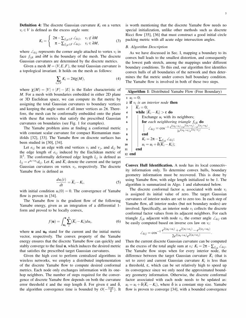
As we have discussed in Sec. I, mapping a boundary to itsconvex hull leads to the smallest distortion, and consequentlythe lowest path stretch, among the mappings under differentboundary conditions. To this end, our algorithm first identifiesconvex hulls of all boundaries of the network and then deter-mines the flat metric under convex hull boundary condition.The Yamabe flow is involved in both of these two steps.

Algorithm 1: Distributed Yamabe Flow (Free Boundary)

ui = 0;1

if vi is an interior node then2

Ki = 0;3

while |Ki −Ki|> ε do4

Exchange ui with its neighbors;5

for each neighboring triangle fi jk do6

∠ki j = cos−1 e2(uk+ui)+e2(ui+u j)−e2(u j+uk)

2e2(uk+ui)e2(ui+u j);7

end8

Ki = 2π−∑ fi jk∠ki j;9

ui = ui +δ(Ki −Ki);10

end11

end12

Convex Hull Identification. A node has its local connectiv-ity information only. To determine convex hulls, boundarygeometry information must be recovered. This is done byusing Yamabe flow, with edge length initialized to be 1. Thealgorithm is summarized in Algo. 1 and elaborated below.

The discrete conformal factor ui associated with node viis assigned its initial value of zero. The target Gaussiancurvatures of interior nodes are set to zero too. In each step ofYamabe flow, all interior nodes (but not boundary nodes) areinvolved. Specifically, an interior node vi collects the discreteconformal factor values from its adjacent neighbors. For eachtriangle fi jk adjacent with node vi, the corner angle ∠ki j canbe easily computed based on inverse cos law on vi:

∠ki j = cos−1 e2(uk+ui)+ e2(ui+u j)− e2(u j+uk)

2e2(uk+ui)e2(ui+u j).

Then the current discrete Gaussian curvature can be computedas the excess of the total angle sum at vi: Ki = 2π−∑ fi jk

∠ki j.The Yamabe flow stops when for every interior node, thedifference between the target Gaussian curvature Ki (that isset to zero) and current Gaussian curvature Ki is less thana threshold, ε, which can be set relatively high to speed upits convergence since we only need the approximated bound-ary geometry information. Otherwise, the discrete conformalfactor associated with each node needs to be updated as:ui = ui +δ(Ki −Ki), where δ is a constant step size. Yamabeflow is proven to converge [34], with a bounded convergence

6

delay of O(− logεδ ). When it stops, a non boundary edge (e.g.,

an edge between nodes vi and v j) has its conformally deformededge length of li j = eui+u j ; for a boundary edge, its edge lengthremains 1.

Next, the new metric (i.e., the calculated edge length) isembedded in a 2D plane via discrete breadth first search.Note that, to determine convex hulls, we do not need a globalembedding; instead, local embedding at boundaries (that havebeen identified in preprocessing) is sufficient. Similar toboundary discovery, a node on a boundary may initiate aprobe message that travels around the boundary. It informsthe boundary nodes that are k hops apart to start embedding.For each of such selected nodes, e.g., node vi, its coordinatesare set to (0,0). Then it arbitrarily selects one of its adjacentneighbors, e.g., v j, and sets its coordinates to (0, li j). To de-termine the coordinates of vk, which is adjacent to both vi andv j, it calculates the intersection points of the two circles withcenters at vi and v j, and radii of lik and l jk, respectively. Then,one of the intersection points that conforms the orientation oftriangle fi jk (that has been determined in preprocessing) ischosen as the coordinates of vk. The procedure continues untilall nodes within k hops have computed their coordinates.

Note that the above embedding is not greedy yet. Thosevirtual coordinates are not useable for greedy routing. Theyare the initial coordinates that reflect the boundary geometricinformation. Based on them, the convex hull for each boundarycan be locally determined by well known algorithms with localmessaging [37].Flat Metric under Convex Boundary Condition. With therecovered boundary geometry information, the desired flatmetric can be computed with Yamabe flow under convexboundary condition. The procedure is similar to the discussionabove for computing the Yamabe flow under free boundarycondition. There are two minor differences only. First we setthe target Gaussian curvatures of all nodes to zero exceptthose on the corners of the convex boundaries. They areset to approximated convex corner angles. Second, boundarynodes will now be involved in computation. In each step ofthe Yamabe flow, the equation to compute current Gaussiancurvature at a boundary node is: Ki = π−∑ fi jk

∠ki j.The same method is employed to determine the flat metric,

and embed it to a 2D plane. But note that the embeddinghere is global. It starts from a node and propagates to theentire network, yielding virtual coordinates for every node.Since this embedding is under convex hull outer boundaryand circle-like convex polygon inner boundary conditions,the established virtual coordinates ensure greedy routing ingeneral. There is only one exception that rarely exists inpractice, but it is discussed below for completeness of ouralgorithm. The exception occurs when a node on an innerconvex boundary is local minimum for a given destination.Our solution is as follows. A message goes around the innerboundary to collect the virtual coordinates of all nodes onthe boundary and compute the average, which serves as theestimated convex center. Then the message goes around theboundary the second time to disseminate this information.

Each node on the boundary computes its distance to thecenter. Using the minimal distance as the radius of a circle,each boundary node calculates its alternative coordinates byprojecting itself onto the circle. The alternative coordinates areused under such rare scenarios only.

IV. ROUTING BASED ON VIRTUAL COORDINATES

Till now each node on the triangular mesh (i.e., a landmark)has obtained its virtual coordinates. Routing between any twosuch nodes is straightforward by using greedy forwarding. Butnote that the triangular mesh is only a sampled backbonerepresentation of the network. Other nodes that are not onthe mesh must be considered too. To this end, each of themcalculates its virtual coordinates in barycentric form, based onthree nearby landmarks. More specifically, consider a triangleT defined by three landmarks vi, v j, and vk. Any node xlocated in this triangle may then be represented as a weightedsum of the three landmarks, i.e., x = α1vi + α2v j + α3vk,where α1 +α2 +α3 = 1. αi is also called area coordinates.It is determined as follows. Let’s connect x and the threelandmarks. The triangle is divided into three sub-triangles. αiis the ratio between each sub-triangle’s area and the wholetriangle’s area. This method is simple and introduces littledistortion as demonstrated in our simulations. In addition,each node keeps the virtual coordinates of its neighboringlandmarks and the hop distances to them.

To deliver a packet, the source node first checks the des-tination’s coordinates via a coordinates lookup service whichis required in all virtual or physical coordinates-based greedyrouting schemes. According to the coordinates of the desti-nation, it chooses a neighboring landmark that is the closestto the destination, and sends its packet toward it. The packetwill be forwarded hop by hop, and in each hop, the aboveprocedure repeats. Note that although the packet is forwardedtoward a neighboring landmark, the actual routing path doesnot have to go through the landmark. In general, when a packetbecomes close to and before it actually reaches a landmark, anintermediate node may discover a new neighboring landmarkthat is now the closest to the destination and thus adjust therouting path to bypass the current landmark. This leads toefficient end-to-end routing, as illustrated in Fig. 4.

L 1

L 2 L 3

L 4

H o l e s

d i

k

m

Fig. 4. Greedy routing based on virtual coordinates, where the routing pathdoes not go through the landmarks.

7

V. SIMULATIONS AND COMPARISON

We implement our proposed Yamabe flow-based schemeand compare it with the harmonic approach [12], hyper-bolic approach [25], Ricci flow-based approach [27], and theshortest path routing. We carried out simulations in wirelesssensor networks with quasi-UDG topologies. Among variousnetworks with different topological shapes being investigated,we notice that the harmonic and hyperbolic approaches mayfail in some of them because the algorithms result in edge flipsor the required computational precision is beyond the capacityof the computer used for simulation.

A. Distortions in Embedding

First, let’s examine several representative networks and thecorresponding embedding results under different algorithms.

Fig. 5 is based on a network with one hole at the bottom.There are about two hundred thousand nodes in the network,among which 1114 nodes are landmarks. For conciseness, onlylandmarks in the mesh structure (or a tree-like structure forhyperbolic embedding) are shown to demonstrate distortionsdue to embedding. For the hyperbolic scheme (see Fig. 5 (c)),a 3-degree tree is employed to realize embedding. We observethat due to the limit in computation precision, we can notembed all nodes in the network to a Poincare disk, becausewith the increase of the depth of the tree, the Euclideandistance between adjacent nodes decreases exponentially. Thecomputation precision soon becomes insufficient to differen-tiate them (64 bits for double type in C++, i.e., 15 decimals,are used in our simulations). So we show the nodes thatcan be embedded only. As can be seen in Fig. 5 (d), Ricciembedding yields a great amount of area distortions (see theclustered area at the top of the inner circle), which has severeimpact on the routing performance (i.e., stretch factor). Theharmonic embedding preserves the relative position of the holeand has less area distortion. But it generates significant angledistortion and some edge distortions along the inner boundary.In addition, it doesn’t avoid local minimums and thus resultingin critical route failures to be discussed later. On the otherhand, Yamabe well preserves the geometry of the originalnetwork, and has the least area distortion. The separate parton the right side of Fig. 5 (e) is a circle embedding for theinner convex hole, which generates alternative coordinates incase a local minimum occurs at a node on the inner convexboundary as discussed in Sec. III.

Networks with more holes are shown in Figs. 6 and 7. Theyboth have about 290 thousand nodes and 1700 landmarks.Harmonic embedding still keeps the relative positions of theholes, but the distortions along the inner boundaries becomehigher; on the other hand, no significant changes in distortionsare observed in Ricci and Yamabe embedding. In addition,since the hyperbolic approach employs a tree for embedding,the actual geometry has no impact on its results.

B. Routing Failures

We study the routing success rate by running greedy routingbetween every pair of nodes in a network. Ricci and Yamabe-

based schemes achieve guaranteed delivery. This has beenverified by our simulations that exhibit 100% success rateunder these two schemes.

Routing failures are observed under the harmonic scheme.The more the holes, the higher the failure rate. For example,4.11% routes fail in the network shown in Fig. 6 (a), whilethe failure rate increases to 4.38% in the network given inFig. 7 (a). With more holes introduced into the network, morenodes may become local minimums for any given destination.Since the harmonic scheme does not completely eliminate suchlocal minimums, more greedy routing failures are observed.We have also studied the impact of the size and the positionof holes by using the networks shown in Figs. 8 and 9,respectively. The harmonic scheme is very sensitive to the sizeof the hole. For example, when the hole enlarges as illustratedin Fig. 8, the routing failure rate increases from 5.4% to15.5%. With the increase of the hole’s size, the perimeter ofthe boundary increases, which results in more local minimumsand accordingly more route failures.

For the hyperbolic approach, we only test the routes betweenthose embedded nodes. Theoretically, the hyperbolic embed-ding is greedy and thus guarantees greedy delivery. However,around 6.13% routing attempts are failed in our simulations.Investigating into such anti-intuitive results, we realize that thefailures are again due to the limited computational precision.Adjacent nodes of the constructed spanning tree have equalhyperbolic distances in Poincare disk, but their Euclidean dis-tances are decreasing almost exponentially. More specifically,the deeper layer a pair of adjacent nodes is from the rootof the tree, the closer their Euclidean distance is in Poincaredisk. After embedding around ten layers of the spanning treein Poincare disk, our computer used for simulation fails to dis-tinguish two nodes with different embedding positions. Notethat since all hyperbolic models are equivalent, any hyperbolicmodel equally requires extremely high computational precisionfor the hyperbolic approach.

Table I summaries the average routing failures of differentschemes on various network topologies shown in Fig. 5(a),Fig. 6(a), Fig. 7(a), Figs. 8, and Figs. 9.

C. Stretch Factor

Stretch factor is a key parameter to evaluate the performanceof greedy routing. It is defined as the ratio between the pathlength in greedy routing and the shortest path length. Weconsider all pairs of nodes (that are greedily routable) in thenetwork and calculate the average stretch factors given inTable II.

TABLE IAVERAGE ROUTING FAILURES OF DIFFERENT SCHEMES ON VARIOUSNETWORK TOPOLOGIES SHOWN IN FIG. 5(A), FIG. 6(A), FIG. 7(A),

FIGS. 8, AND FIGS. 9.

Schemes Hyperbolic Harmonic Ricci Yamabe

Average routing failure 6.13% 5.75% 0 0

8

(a) (b) (c) (d) (e)

Fig. 5. (a) Original topology with one concave hole; (b) Harmonic embedding with angle and area distortion along the inner boundary; (c) Hyperbolicembedding; (d) Ricci embedding with severe area distortion above the inner circle; (e) Yamabe embedding with well preserved geometry and least areadistortion. The part on the right side is a circle embedding for the inner convex hole, which generates alternative coordinates in case two sides of the innerconvex boundary are perfectly parallel as discussed in Sec. III.

(a) (b) (c) (d) (e)

Fig. 6. (a) Original topology with two concave holes; (b) Harmonic embedding; (c) Hyperbolic embedding; (d) Ricci embedding; (e) Yamabe embedding.

(a) (b) (c) (d) (e)

Fig. 7. (a) Original topology with three concave holes; (b) Harmonic embedding; (c) Hyperbolic embedding; (d) Ricci embedding; (e) Yamabe embedding.

The hyperbolic scheme relies on the shortest path tree rootedat one node in the network. As a result, two adjacent nodesmay have a long routing path, leading to poor stretch factor.We observe that Ricci experiences high and unstable stretchfactor. As discussed above, in the first topology (Fig. 5(a)),Ricci exhibits severe distortions, resulting in a stretch factoras high as over 1.8. In the second and third topologies, thedistortions are reduced, and thus yielding moderate stretch.The stretch factor under harmonic embedding is stable andlow. But recall that it pays the price of many routing failures.Our proposed Yamabe flow-based scheme achieves not onlythe lowest but also the stablest stretch factor, always between1.3 and 1.4 in all of our experiments.

The size of the hole does not noticeably affect the stretchfactor under Ricci, harmonic, or Yamabe. As a matter of fact,the stretch factor actually decreases slightly in both Ricci and

Yamabe-based schemes, when the hole enlarges (see Fig. 8).As another interesting observation, we find Ricci is sensitive

to the position of the hole. For example, consider threepositions at corner, bottom and center illustrated in Fig. 9.Ricci performs better when the hole is at the center (achievinga stretch factor of 1.4), while its stretch factor increases to 1.5when the hole locates at border or corner. This phenomenon isbecause Ricci always maps the largest hole (in this case onlyone hole) to the center. When the original position of the holeis far away from the center, it results in large compression andstretching of the edges around the hole. On the other hand,Yamabe and Harmonic are not affected much by the hole’sposition.

The stretch factor distribution is illustrated in Fig. 10. Thisis obtained in the network shown in Fig. 5(a). We observesimilar statistics in other networks. As can be seen, Ricci

9

Fig. 8. Two networks with a hole of increasing size. Fig. 9. Three networks with a hole at corner, bottom, and center, respectively.

results in many routes with their stretch factors greater than1.8, while the stretch factors of Harmonic and Yamabe arenicely distributed at a lower range.

D. 3D Surface

To demonstrate our proposed approach on 3D surfaces, weadopt a real 3D surface data set (UTM zone 15 of North Amer-ican Datum 1983). It was distributed by “Atlas: The LouisianaStatewide GIS”, LSU CADGIS Research Laboratory, BatonRouge, LA. We choose an area of 1km×1km, with a heightvariation of 40m and a resolution of 5m, as shown in Fig. 11.The area includes hills and water ponds. Since the points ofthe data set are on a grid structure, we assume the sensorsare placed at a grid too, where adjacent nodes are 20m apart.It is straightforward to establish a mesh structure and applythe Yamabe flow-based embedding. Our results show a stretchfactor of 1.36 and 100% delivery between all pairs of nodes.

VI. CONCLUSION

In this paper we have proposed a distributed Yamabe flow-based scheme to enable greedy routing in large scale wirelessnetworks deployed on 2D and 3D surfaces. It identifies theconvex hull of each boundary and employs Yamabe flow tocompute flat metric under convex hull boundary condition toestablish virtual coordinates. Such virtual coordinates are usedfor greedy routing. Since the proposed embedding algorithmmaps the outer boundary to a convex shape and an interiorconcave void to a circle-like convex polygon, it effectivelyeliminates local minimum and attains guaranteed delivery.At the same time, it introduces a small distortion only andconsequently achieves a low stretch factor. Our simulationshave shown that its stretch factor is lower than any existinggreedy embedding algorithms. Moreover, the proposed schemeis merely based on local connectivity and consumes a smallconstant storage, thus scaling to arbitrarily large networks.

TABLE IIAVERAGE STRETCH FACTORS OF DIFFERENT SCHEMES.

Scenario Hyperbolic Harmonic Ricci Yamabe

Topology 1 (Fig. 5(a)) 1.65606 1.45715 1.83518 1.38846Topology 2 (Fig. 6(a)) 1.65501 1.46334 1.54808 1.39032Topology 3 (Fig. 7(a)) 1.64974 1.48278 1.55544 1.38717

ACKNOWLEDGEMENTS.

H. Wu is partially supported by NSF CNS-1018306 andCNS-1320931. M. Jin is partially supported by NSF CCF-1054996, CNS-1018306 and CNS-1320931.

REFERENCES

[1] I. Stojmenovic, “Machine-to-Machine Communications with In-networkData Aggregation, Processing and Actuation for Large Scale Cyber-Physical Systems,” IEEE Internet of Things Journal, 2014.

[2] P. Bose, P. Morin, I. Stojmenovic, and J. Urrutia, “Routing withGuaranteed Delivery in Ad Hoc Wireless Networks,” in Proc. of ThirdInternational Workshop Discrete Algorithms and Methods for MobileComputing and Communications, pp. 48–55, 1999.

[3] B. Karp and H. Kung, “GPSR: Greedy Perimeter Stateless Routing forWireless networks,” in Proc. of The ACM/IEEE International Conferenceon Mobile Computing and Networking (MobiCom), pp. 1–12, 2001.

[4] E. Kranakis, H. Singh, and J. Urrutia, “Compass Routing on GeometricNetworks,” in Proc. of The 11th Canadian Conference on ComputationalGeometry (CCCG’99), pp. 51–54, 1999.

[5] F. Kuhn, R. Wattenhofer, Y. Zhang, and A. Zollinger, “Geometric Ad-hocRouting: Theory and Practice,” in Proc. of The 22nd ACM InternationalSymposium on the Principles of Distributed Computing (PODC’03),pp. 63–72, 2003.

[6] F. Kuhn, R. Wattenhofer, and A. Zollinger, “Worst-case Optimal andAverage-case Efficient Geometric Ad-hoc Routing,” in Proc. of ACMInternational Symposium on Mobile Ad hoc Networking and Computing(MobiHOC), pp. 267–278, 2003.

[7] B. L. S. Mitra and B. Liskov, “Path Vector Face Routing: GeographicRouting with Local Face Information,” in Proc. of ICNP, 2005.

[8] H. Frey and I. Stojmenovic, “On Delivery Guarantees of Face andCombined Greedy-face Routing in Ad Hoc and Sensor Networks,” inProc. of The ACM/IEEE International Conference on Mobile Computingand Networking (MobiCom), pp. 390–401.

[9] G. Tan, M. Bertier, and A.-M. Kermarrec, “Visibility-Graph-basedShortest-Path Geographic Routing in Sensor Networks,” in Proc. of IEEEInternational Conference on Computer Communications (INFOCOM),2009.

[1.0,1.2) [1.2,1.4) [1.4,1.6) [1.6,1.8) [1.8,2.0) [2.0,2.2) [2.2,2.4) >=2.40

0.05

0.1

0.15

0.2

0.25

0.3

0.35

0.4

0.45

Stretch Factor

Pe

rce

nt o

f R

ou

tes

Ricci

Yamabe

Harmonic

Fig. 10. Stretch factor distribution of Ricci, Yamabe and Harmonic.

10

Fig. 11. A 3D surface (UTM zone 15 of North American Datum 1983) inan area of 1km×1km, with a height variation of 40m and a resolution of 5m.

[10] S. Funke and N. Milosavljevic, “Guaranteed-Delivery Geographic Rout-ing Under Uncertain Node Locations,” in Proc. of IEEE InternationalConference on Computer Communications (INFOCOM), pp. 1244–1252,2007.

[11] C. Liu and J. Wu, “Efficient Geometric Routing in Three DimensionalAd Hoc Networks,” in Proc. of IEEE International Conference onComputer Communications (INFOCOM), 2009.

[12] A. Rao, S. Ratnasamy, C. Papadimitriou, S. Shenker, and I. Stoica,“Geographic Routing without Location Information,” in Proc. of TheACM/IEEE International Conference on Mobile Computing and Net-working (MobiCom), pp. 96–108, 2003.

[13] R. Fonseca, S. Ratnasamy, J. Zhao, C. T. Ee, D. Culler, S. Shenker, andI. Stoica, “Beacon Vector Routing: Scalable Point-to-Point Routing inWireless Sensornets,” in Proc. of The Second USENIX/ACM Symposiumon Networked Systems Design and Implementation (NSDI’05), 2005.

[14] Y. Zhao, B. Li, Q. Zhang, Y. Chen, and W. Zhu, “Efficient Hop ID basedRouting for Sparse Ad Hoc Networks,” in Proc. of ICNP, pp. 179–190,2005.

[15] Q. Cao and T. Abdelzaher, “Scalable logical coordinates frameworkfor routing in wireless sensor networks,” ACM Transactions on SensorNetworks, vol. 2, no. 4, pp. 557–593, 2006.

[16] A. Caruso, S. Chessa, S. De, and A. Urpi, “GPS Free CoordinateAssignment and Routing in Wireless Sensor Networks,” in Proc. of IEEEInternational Conference on Computer Communications (INFOCOM),pp. 150–160, 2005.

[17] S. Tao, A. Ananda, and M. C. Chan, “Greedy Hop Distance RoutingUsing Tree Recovery on Wireless Ad Hoc and Sensor Networks,” inProc. of IEEE International Conference on Communications (ICC’08),pp. 2712–2716, 2008.

[18] M. J. Tsai, H. Y. Yang, and W. Q. Huang, “Axis Based Virtual Coordi-nate Assignment Protocol and Delivery Guaranteed Routing Protocol inWireless Sensor Networks,” in Proc. of IEEE International Conferenceon Computer Communications (INFOCOM), pp. 2234–2242, 2007.

[19] K. Liu and N. Abu-Ghazaleh, “Stateless and Guaranteed GeometricRouting on Virtual Coordinate Systems,” in Proc. of The 5th IEEE Inter-national Conference on Mobile Ad Hoc and Sensor Systems (MASS’08),pp. 340–346, 2008.

[20] Q. Fang, J. Gao, L. J. Guibas, V. Silva, and L. Zhang, “GLIDER:Gradient Landmark-based Distributed Routing for Sensor Networks,” inProc. of IEEE International Conference on Computer Communications(INFOCOM), pp. 339–350, 2005.

[21] G. Tan, M. Bertier, and A.-M. Kermarrec, “Convex Partition of SensorNetworks and Its Use in Virtual Coordinate Geographic Routing,” inProc. of IEEE International Conference on Computer Communications(INFOCOM), 2009.

[22] C. Papadimitriou and D. Ratajczak, “On A Conjecture Related toGeometric Routing,” Theoretical Computer Science, vol. 344, no. 1,pp. 3–14, 2005.

[23] P. Angelini, F. Frati, and L. Grilli, “An Algorithm to Construct GreedyDrawings of Triangulations,” in Proc. of The 16th International Sympo-sium on Graph Drawing, pp. 26–37, 2008.

[24] T. Leighton and A. Moitra, “Some Results on Greedy Embeddingsin Metric Spaces,” in Proc. of The 49th IEEE Annual Symposium onFoundations of Computer Science, pp. 337–346, 2008.

[25] R. Kleinberg, “Geographic Routing Using Hyperbolic Space,” in Proc.

of IEEE International Conference on Computer Communications (IN-FOCOM), pp. 1902–1909, 2007.

[26] A. Cvetkovski and M. Crovella, “Hyperbolic Embedding and Routingfor Dynamic Graphs,” in Proc. of IEEE International Conference onComputer Communications (INFOCOM), 2009.

[27] R. Sarkar, X. Yin, J. Gao, F. Luo, and X. D. Gu, “Greedy routing withguaranteed delivery using ricci flows,” in Proc. of The 8th InternationalSymposium on Information Processing in Sensor Networks (IPSN’09),pp. 121–132, April 2009.

[28] R. Flury, S. Pemmaraju, and R. Wattenhofer, “Greedy Routing withBounded Stretch,” in Proc. of IEEE International Conference on Com-puter Communications (INFOCOM), 2009.

[29] Y.-L. Yang, J. Kim, F. Luo, S.-M. Hu, and X. Gu, “Optimal SurfaceParameterization Using Inverse Curvature Map,” IEEE Tran. on Visual-ization and Computer Graphics, vol. 14, no. 5, pp. 1054–1066, 2008.

[30] B. Springborn, P. Schroder, and U. Pinkall, “Conformal Equivalence ofTriangle Meshes,” in ACM SIGGRAPH, pp. 1–11, 2008.

[31] S. Funke and N. Milosavljevi, “How Much Geometry Hides in Con-nectivity? - Part II,” in Proc. of The Eighteenth Annual ACM-SIAMSymposium on Discrete Algorithms (SODA’07), pp. 958–967, 2007.

[32] H. Yamabe, “The Yamabe Problem,” Osaka Math. J., vol. 12, no. 1,pp. 21–37, 1960.

[33] J. M. Lee and T. H. Parker, “The Yamabe Problem,” Bulletin of theAmerican Mathematical Society, vol. 17, no. 1, pp. 37–91, 1987.

[34] F. Luo, “Combinatorial Yamabe Flow on Surfaces,” Commun. Contemp.Math., vol. 6, no. 5, pp. 765–780, 2004.

[35] B. Chow and F. Luo, “Combinatorial Ricci Flows on Surfaces,” JournalDifferential Geometry, vol. 63, no. 1, pp. 97–129, 2003.

[36] M. Jin, J. Kim, F. Luo, and X. Gu, “Discrete Surface Ricci Flow,” IEEETran. on Visualization and Computer Graphics, vol. 14, no. 5, pp. 1030–1043, 2008.

[37] M. Berg, O. Cheong, M. Kreveld, and M. Overmars, ComputationalGeometry: Algorithms and Applications (3rd Ed.). Springer, 2008.