reducing packet transmission delay in vehicular ad hoc networks using edge node based greedy routing

K.Prasanth, K.Duraiswamy, K.Jayasudha & C.Chandrasekar

International Journal of Computer Networks , Volume (2): Issue (1) 1

Reducing Packet Transmission Delay in Vehicular Ad Hoc Networks using Edge Node Based Greedy Routing

K.Prasanth [email protected] Research Scholar, Department of IT K.S.Rangasamy College of Technology Tiruchengode-637215, Tamilnadu, India

Dr.K.Duraiswamy [email protected] Dean Academic, Department of CSE K.S.Rangasamy College of Technology Tiruchengode-637215, Tamilnadu, India

K.Jayasudha [email protected] Research Scholar, Department of MCA K.S.R College of Engineering Tiruchengode-637215, Tamilnadu, India

Dr.C.Chandrasekar [email protected] Reader, Department of MCA Periyar University Salem, Tamilnadu, India

Abstract

VANETs (Vehicular Ad hoc Networks) are highly mobile wireless ad hoc networks and will play an important role in public safety communications and commercial applications. Routing of data in VANETs is a challenging task due to rapidly changing topology and high speed mobility of vehicles. Conventional routing protocols in MANETs (Mobile Ad hoc Networks) are unable to fully address the unique characteristics in vehicular networks. In this paper, we propose a potential EBGR (Edge Node Based Greedy Routing), a greedy position based routing approach to forward packets to the node present in the edge of the transmission range of source/forwarding node. The most suitable next hop is selected based on potential score of neighbor node. We propose Revival Mobility model (RMM) to evaluate the performance of our routing technique. This paper presents a detailed description of our approach and simulation results using ns2.27 show that end to end delay in packet transmission is minimized considerably compared to current routing protocols of VANET. Keywords: Vehicular Ad hoc Networks, Greedy Position Based Routing, Potential EBGR, Revival Mobility

Model, End to End delay. .

1. INTRODUCTION

Vehicular Ad hoc Networks (VANETs) are based on short range wireless communications (e.g., IEEE 802.11) for the use in road safety and many other commercial applications. The Federal



Communications Commission (FCC) has allocated 75 MHz in 5.9 GHz band for licensed Dedicated Short Range Communication (DSRC) for vehicle-to-vehicle and vehicle to infrastructure communications. The radio range of VANETs is several hundred meters, typically between 250 and 300 meters. It is expected that more vehicles would be equipped with computing and wireless communication devices in the near future. We assume that vehicles should be equipped with wireless communication devices, GPS, digital maps, and optional sensors for reporting vehicle conditions. Vehicles exchange information with other vehicles as well as road-side infrastructures within their radio ranges. A vehicular network is a mobile ad hoc network and its characteristics can be summarized as high dynamics, mobility constraints, predicable mobility, large scale and energy constraints are not that high as every vehicle has a large enough battery capacity.

2. RELATED WORK

In this section, we briefly summarize the characteristics of VANETs related to routing and also we will survey the existing routing schemes in both MANETs and VANETs in vehicular environments. 2.1. VANETs Characteristics In the following, we only summarize the uniqueness related to routing of VANETs compared with MANETs. Unlimited transmission power: Mobile device power issues are not a significant constraint in vehicular Networks. Since the vehicle itself can provide continuous power to computing and communication devices. High computational capability: Operating vehicles can afford significant computing, communication and sensing capabilities. Highly dynamic topology: Vehicular network scenarios are very different from classic ad hoc networks. In VANETs, vehicles can move fast. It can join and leave the network much more frequently than MANETs. Since the radio range is small compared with the high speed of vehicles (typically, the radio range is only 250 meters while the speed for vehicles in freeway will be 30m/s). This indicates the topology in VANETs changes much more frequently. Predicable Mobility: Unlike classic mobile ad hoc networks, where it is hard to predict the nodes’ mobility, vehicles tend to have very predictable movements that are (usually) limited to roadways. The movement of nodes in VANETs is constrained by the layout of roads. Roadway information is often available from positioning systems and map based technologies such as GPS. Each pair of nodes can communicate directly when they are within the radio range. Potentially large scale: Unlike most ad hoc networks studied in the literature that usually assume a limited network size, vehicular networks can in principle extend over the entire road network and so include many participants. Partitioned network: Vehicular networks will be frequently partitioned. The dynamic nature of traffic may result in large inter vehicle gaps in sparsely populated scenarios and hence in several isolated clusters of nodes. Network connectivity: The degree to which the network is connected is highly dependent on two factors: the range of wireless links and the fraction of participant vehicles, where only a fraction of vehicles on the road could be equipped with wireless interfaces. 2.2 Routing protocols in MANET The routing protocols in MANETs can be classified by their properties. On one hand, they can be classified into two categories, proactive and reactive. Proactive algorithms employ classical routing strategies such as distance-vector routing (e.g., DSDV [1]) or link-state routing (e.g., OLSR [2] and TBRPF [3]). They maintain routing information about the available paths in the network even if these paths are not currently used. The main drawback of these approaches is that the maintenance of unused paths may occupy a significant



part of the available bandwidth if the topology of the network changes frequently [4]. Since a network between cars is extremely dynamic we did not further investigate proactive approaches. Reactive routing protocols such as DSR [5], TORA [6], and AODV [7] maintain only the routes that are currently in use, thereby reducing the burden on the network when only a small subset of all available routes is in use at any time. It can be expected that communication between cars will only use a very limited number of routes, therefore reactive routing seems to fit this application scenario. As a representative of the reactive approaches we have chosen DSR, since it has been shown to be superior to many other existing reactive ad-hoc routing protocols in [8]. Position-based routing algorithms require that information about the physical position of the participating nodes be available. This position is made available to the direct neighbours in form periodically transmitted beacons. A sender can request the position of a receiver by means of a location service. The routing decision at each node is then based on the destination’s position contained in the packet and the position of the forwarding node’s neighbours. Position-based routing does thus not require the establishment or maintenance of routes. Examples for position-based routing algorithms are face-2 [9], GPSR [10], DREAM [11] and terminodes routing [12]. As a representative of the position based algorithms we have selected GPSR, (which is algorithmically identical to face-2), since it seems to be scalable and well suited for very dynamic networks. 2.3. Routing protocols in VANET Following are a summary of representative VANETs routing algorithms . GSR (Geographic Source Routing): Lochert et al. in [13] proposed GSR, a position-based routing with topological information. This approach employs greedy forwarding along a pre-selected shortest path. The simulation results show that GSR outperforms topology based approaches (AODV and DSR) with respect to packet delivery ratio and latency by using realistic vehicular traffic. But this approach neglects the case that there are not enough nodes for forwarding packets when the traffic density is low. Low traffic density will make it difficult to find an end-to-end connection along the pre-selected path. GPCR (Greedy Perimeter Coordinator Routing): To deal with the challenges of city scenarios, Lochert et al. designed GPCR in [14]. This protocol employs a restricted greedy forwarding procedure along a preselected path. When choosing the next hop, a coordinator (the node on a junction) is preferred to a non coordinator node, even if it is not the geographical closest node to destination. Similar to GSR, GPCR neglects the case of low traffic density as well. A-STAR (Anchor-based Street and Traffic Aware Routing): To guarantee an end-to-end connection even in a vehicular network with low traffic density, Seet et al. proposed A-STAR [15]. A-STAR uses information on city bus routes to identify an anchor path with high connectivity for packet delivery. By using an anchor path, A-STAR guarantees to find an end-to-end connection even in the case of low traffic density. This position-based scheme also employs a route recovery strategy when the packets are routed to a local optimum by computing a new anchor path from local maximum to which the packet is routed. The simulation results show A-STAR achieves obvious network performance improvement compared with GSR and GPSR. But the routing path may not be optimal because it is along the anchor path. It results in large delay. MDDV (Mobility-Centric Data Dissemination Algorithm for Vehicular Networks): To achieve reliable and efficient routing, Wu et al. proposed MDDV [16] that combines opportunistic forwarding, geographical forwarding, and trajectory-based forwarding. MDDV takes into account the traffic density. A forwarding trajectory is specified extending from the source to the destination (trajectory-based forwarding), along which a message will be moved geographically closer to the destination (geographical forwarding). The selection of forwarding trajectory uses the geographical knowledge and traffic density. MDDV assumes the traffic density is static.



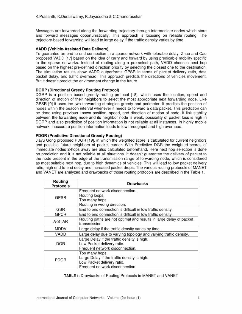
Messages are forwarded along the forwarding trajectory through intermediate nodes which store and forward messages opportunistically. This approach is focusing on reliable routing. The trajectory-based forwarding will lead to large delay if the traffic density varies by time. VADD (Vehicle-Assisted Data Delivery) To guarantee an end-to-end connection in a sparse network with tolerable delay, Zhao and Cao proposed VADD [17] based on the idea of carry and forward by using predicable mobility specific to the sparse networks. Instead of routing along a pre-select path, VADD chooses next hop based on the highest pre-defined direction priority by selecting the closest one to the destination. The simulation results show VADD outperforms GPSR in terms of packet delivery ratio, data packet delay, and traffic overhead. This approach predicts the directions of vehicles movement. But it doesn’t predict the environment change in the future. DGRP (Directional Greedy Routing Protocol) DGRP is a position based greedy routing protocol [18], which uses the location, speed and direction of motion of their neighbors to select the most appropriate next forwarding node. Like GPSR [9] it uses the two forwarding strategies greedy and perimeter. It predicts the position of nodes within the beacon interval whenever it needs to forward a data packet. This prediction can be done using previous known position, speed, and direction of motion of node. If link stability between the forwarding node and its neighbor node is weak, possibility of packet loss is high in DGRP and also prediction of position information is not reliable at all instances. In highly mobile network, inaccurate position information leads to low throughput and high overhead. PDGR (Predictive Directional Greedy Routing) Jiayu Gong proposed PDGR [19], in which the weighted score is calculated for current neighbors and possible future neighbors of packet carrier. With Predictive DGR the weighted scores of immediate nodes 2-hops away are also calculated beforehand. Here next hop selection is done on prediction and it is not reliable at all situations. It doesn’t guarantee the delivery of packet to the node present in the edge of the transmission range of forwarding node, which is considered as most suitable next hop, due to high dynamics of vehicles. This will lead to low packet delivery ratio, high end to end delay and increased packet drops. The various routing protocols of MANET and VANET are analyzed and drawbacks of those routing protocols are described in the Table 1.

Routing Protocols

Drawbacks

GPSR

Frequent network disconnection. Routing loops. Too many hops. Routing in wrong direction.

GSR End to end connection is difficult in low traffic density.

GPCR End to end connection is difficult in low traffic density.

A-STAR Routing paths are not optimal and results in large delay of packet transmission

MDDV Large delay if the traffic density varies by time.

VADD Large delay due to varying topology and varying traffic density.

DGR Large Delay if the traffic density is high. Low Packet delivery ratio. Frequent network disconnection.

PDGR

Too many hops. Large Delay if the traffic density is high. Low Packet delivery ratio. Frequent network disconnection

TABLE 1: Drawbacks of Routing Protocols in MANET and VANET



3. PROPOSED ROUTING ALGORITHM

3.1 Edge Node Based Greedy Routing Algorithm (EBGR) EBGR is a reliable greedy position base routing algorithm designed for sending messages from any node to any other node (unicast) or from one node to all other nodes (broadcast/multicast) in a vehicular ad hoc network. The general design goals of the EBGR algorithm are to optimize the packet behavior for ad hoc networks with high mobility and to deliver messages with high reliability. The EBGR algorithm has six basic functional units. First is Neighbor Node Identification (NNI), second is Distance Calculation (DC), third is Direction of Motion Identification (DMI), fourth is Reckoning Link Stability (RLS), fifth is Potential score calculation (PS) and sixth is Edge Node Selection (ENS). The NNI is responsible for collection of information of all neighbor nodes present within the transmission range of source/forwarder node at any time. The DC is responsible for calculating the closeness of next hop using distance information from the GPS. DMI is responsible to identify the direction of motion of neighbor nodes which is moving towards the direction of destination. The RLS is responsible for identifying link stability between the source/forwarder node and its neighbor nodes. The PS is responsible to calculate potential score and identifies the neighbor node having higher potential for further forwarding of a particular packet to destination. The ENS is responsible to select an edge node having higher potential score in different levels of transmission range. In the following section, the general assumptions of EBGR algorithm are briefly discussed and then functional units of EBGR algorithm are discussed in detail.

3.2 Assumptions The algorithm design is based on the following assumptions: All nodes are equipped with GPS receivers, digital maps, optional sensors and On Board Units (OBU). Location information of all vehicles/nodes can be identified with the help of GPS receivers. The only communications paths available are via the ad-hoc network and there is no other communication infrastructure. Node power is not the limiting factor for the design. Communications are message oriented. The Maximum Transmission Range (MTR) of each node in the environment is 250m. 3.3. Neighbor Node Identification (NNI) Neighbor node identification is the process whereby a vehicle/node identifies its current neighbors within its transmission range. For a particular vehicle, any other vehicle that is within its radio transmission range is called a neighbor. All vehicles consist of neighbor set which holds details of its neighbor vehicles. Since all nodes might be moving, the neighbors for a particular mobile node are always changing. The neighbor set is dynamic and needs to be updated frequently. Generally, neighbor node identification is realized by using periodic beacon messages. The beacon message consists of node ID, node location and timestamp. Each node informs other nodes of its existence by sending out beacon message periodically. All nodes within the transmission range of source/packet forwarding node will intimate its presence by sending a beacon message every µ second. After the reception of a beacon, each node will update its

neighbor set table. If a node position is changed, then it will update its position to all neighbors by sending beacon signal. If a known neighbor, times out after α * µ seconds without having

received a beacon (α is the number of beacons that a node is allowed to miss) and it will be

removed from the neighbor set table.

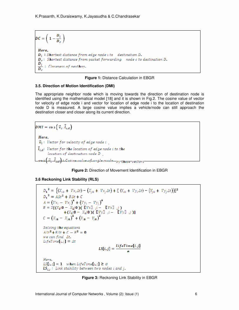
3.4. Distance calculation (DC) The location and distance information of all vehicles/nodes can be identified with the help of GPS receivers. It can be communicated to neighbor vehicles using periodic beacon messages. The neighbor node which is closer to the destination node is calculated. The closeness of next hop is identified by the mathematical model [18] and it is shown in Fig.1.



Figure 1: Distance Calculation in EBGR

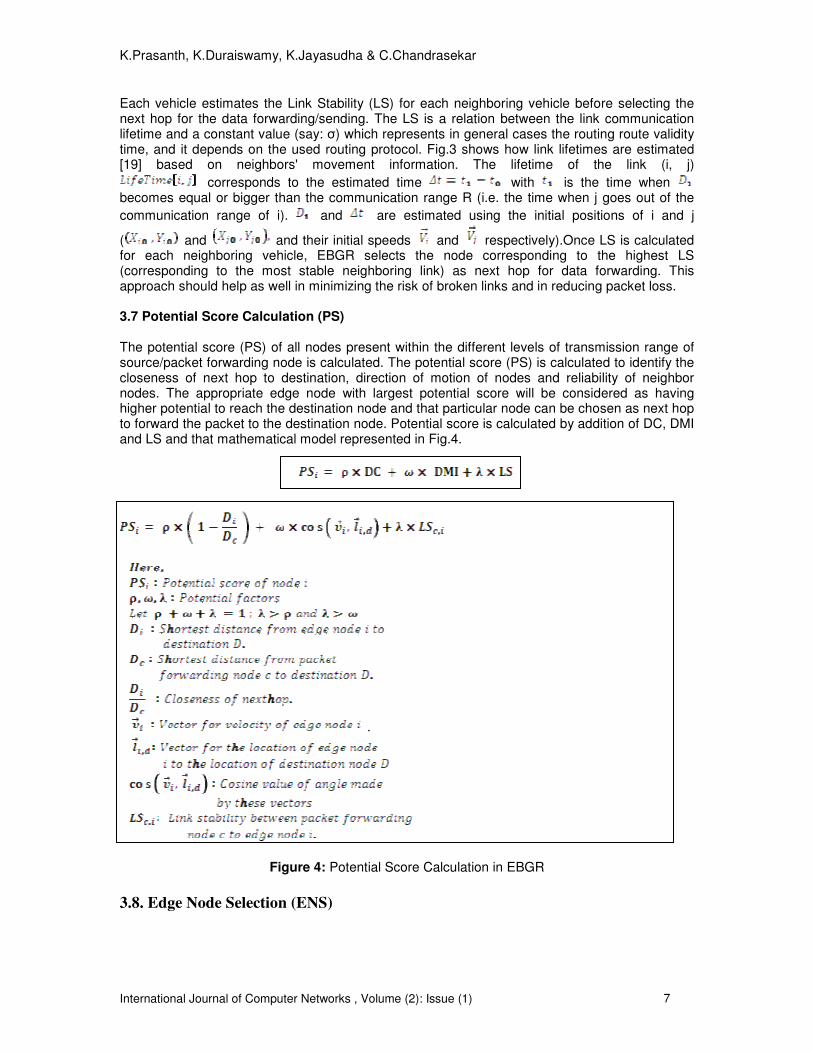
3.5. Direction of Motion Identification (DMI)

The appropriate neighbor node which is moving towards the direction of destination node is identified using the mathematical model [18] and it is shown in Fig.2. The cosine value of vector for velocity of edge node i and vector for location of edge node i to the location of destination node D is measured. A large cosine value implies a vehicle/node can still approach the destination closer and closer along its current direction.

.

.

Figure 2: Direction of Movement Identification in EBGR

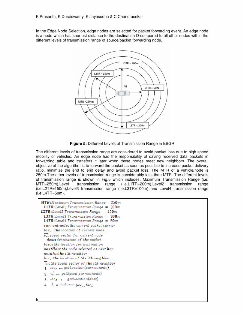
3.6 Reckoning Link Stability (RLS)

Figure 3: Reckoning Link Stability in EBGR



Each vehicle estimates the Link Stability (LS) for each neighboring vehicle before selecting the next hop for the data forwarding/sending. The LS is a relation between the link communication lifetime and a constant value (say: σ) which represents in general cases the routing route validity time, and it depends on the used routing protocol. Fig.3 shows how link lifetimes are estimated [19] based on neighbors' movement information. The lifetime of the link (i, j)

corresponds to the estimated time with is the time when becomes equal or bigger than the communication range R (i.e. the time when j goes out of the

communication range of i). and are estimated using the initial positions of i and j

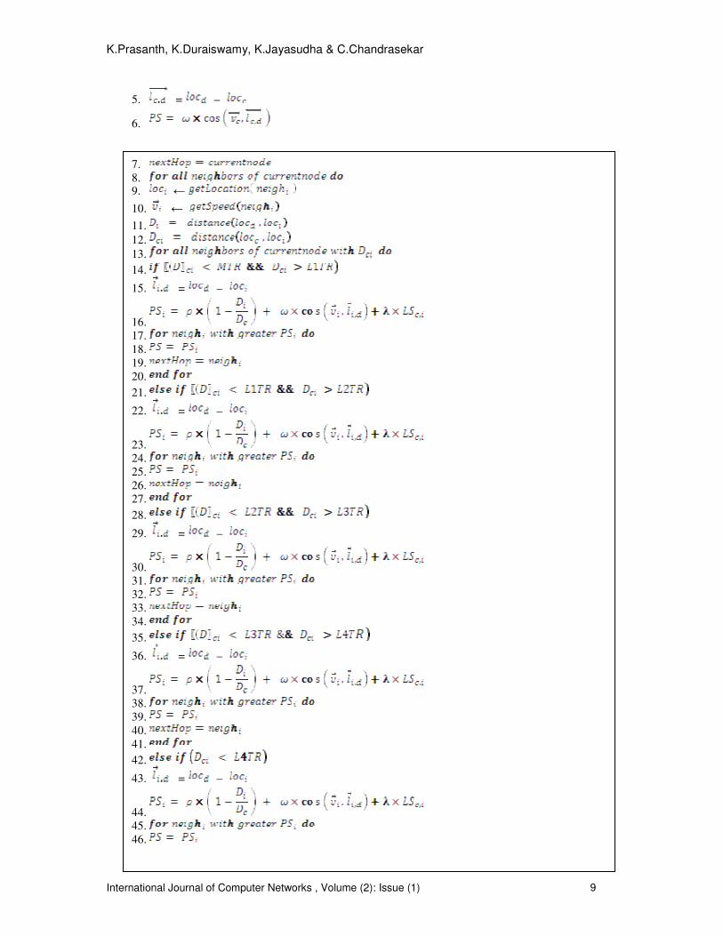
( and and their initial speeds and respectively).Once LS is calculated for each neighboring vehicle, EBGR selects the node corresponding to the highest LS (corresponding to the most stable neighboring link) as next hop for data forwarding. This approach should help as well in minimizing the risk of broken links and in reducing packet loss. 3.7 Potential Score Calculation (PS) The potential score (PS) of all nodes present within the different levels of transmission range of source/packet forwarding node is calculated. The potential score (PS) is calculated to identify the closeness of next hop to destination, direction of motion of nodes and reliability of neighbor nodes. The appropriate edge node with largest potential score will be considered as having higher potential to reach the destination node and that particular node can be chosen as next hop to forward the packet to the destination node. Potential score is calculated by addition of DC, DMI and LS and that mathematical model represented in Fig.4.

.

Figure 4: Potential Score Calculation in EBGR

3.8. Edge Node Selection (ENS)



In the Edge Node Selection, edge nodes are selected for packet forwarding event. An edge node is a node which has shortest distance to the destination D compared to all other nodes within the different levels of transmission range of source/packet forwarding node.

Figure 5: Different Levels of Transmission Range in EBGR

The different levels of transmission range are considered to avoid packet loss due to high speed mobility of vehicles. An edge node has the responsibility of saving received data packets in forwarding table and transfers it later when those nodes meet new neighbors. The overall objective of the algorithm is to forward the packet as soon as possible to increase packet delivery ratio, minimize the end to end delay and avoid packet loss. The MTR of a vehicle/node is 250m.The other levels of transmission range is considerably less than MTR. The different levels of transmission range is shown in Fig.5 which includes, Maximum Transmission Range (i.e. MTR=250m),Level1 transmission range (i.e.L1TR=200m),Level2 transmission range (i.e.L2TR=150m),Level3 transmission range (i.e.L3TR=100m) and Level4 transmission range (i.e.L4TR=50m).

1. ←

2. ←

3. ←

4. = (locc , locd)



5. = –

6.

7.

8. 9. ←

10. ←

11.

12.

13.

14.

15. = –

16. 17.

18.

19.

20.

21.

22. = –

23. 24.

25.

26.

27.

28.

29. = –

30. 31.

32.

33.

34.

35.

36. = –

37. 38.

39.

40.

41.

42.

43. = –

44. 45.

46.



47.

48.

49.

50.

51.

52.

53.

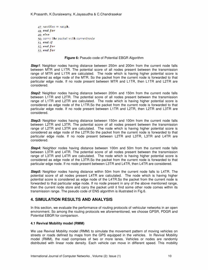
Figure 6: Pseudo code of Potential EBGR Algorithm

Step1: Neighbor nodes having distance between 250m and 200m from the current node falls between MTR and L1TR. The potential score of all nodes present between the transmission range of MTR and L1TR are calculated. The node which is having higher potential score is considered as edge node of the MTR. So the packet from the current node is forwarded to that particular edge node. If no node present between MTR and L1TR, then L1TR and L2TR are considered. Step2: Neighbor nodes having distance between 200m and 150m from the current node falls between L1TR and L2TR. The potential score of all nodes present between the transmission range of L1TR and L2TR are calculated. The node which is having higher potential score is considered as edge node of the L1TR.So the packet from the current node is forwarded to that particular edge node. If no node present between L1TR and L2TR, then L2TR and L3TR are considered. Step3: Neighbor nodes having distance between 150m and 100m from the current node falls between L2TR and L3TR. The potential score of all nodes present between the transmission range of L2TR and L3TR are calculated. The node which is having higher potential score is considered as edge node of the L2TR.So the packet from the current node is forwarded to that particular edge node. If no node present between L2TR and L3TR, L3TR and L4TR are considered. Step4: Neighbor nodes having distance between 100m and 50m from the current node falls between L3TR and L4TR. The potential score of all nodes present between the transmission range of L3TR and L4TR are calculated. The node which is having higher potential score is considered as edge node of the L3TR.So the packet from the current node is forwarded to that particular edge node. If no node present between L3TR and L4TR, then L4TR are considered. Step5: Neighbor nodes having distance within 50m from the current node falls to L4TR. The potential score of all nodes present L4TR are calculated. The node which is having higher potential score is considered as edge node of the L4TR.So the packet from the current node is forwarded to that particular edge node. If no node present in any of the above mentioned range, then the current node store and carry the packet until it find some other node comes within its transmission range. The pseudo code of ENS algorithm is illustrated in Fig.6.

4. SIMULATION RESULTS AND ANALYSIS In this section, we evaluate the performance of routing protocols of vehicular networks in an open environment. So among the routing protocols we aforementioned, we choose GPSR, PDGR and Potential EBGR for comparison. 4.1 Revival Mobility model (RMM) We use Revival Mobility model (RMM) to simulate the movement pattern of moving vehicles on streets or roads defined by maps from the GPS equipped in the vehicles. In Revival Mobility model (RMM), the road comprises of two or more lanes. Vehicles or nodes are randomly distributed with linear node density. Each vehicle can move in different speed. This mobility



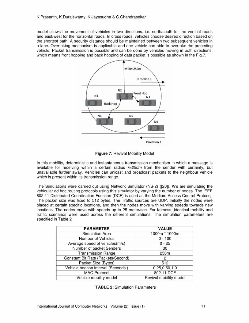
model allows the movement of vehicles in two directions. i.e. north/south for the vertical roads and east/west for the horizontal roads. In cross roads, vehicles choose desired direction based on the shortest path. A security distance should be maintained between two subsequent vehicles in a lane. Overtaking mechanism is applicable and one vehicle can able to overtake the preceding vehicle. Packet transmission is possible and can be done by vehicles moving in both directions, which means front hopping and back hopping of data packet is possible as shown in the Fig.7.

Figure 7: Revival Mobility Model In this mobility, deterministic and instantaneous transmission mechanism in which a message is available for receiving within a certain radius r=250m from the sender with certainty, but unavailable further away. Vehicles can unicast and broadcast packets to the neighbour vehicle which is present within its transmission range. The Simulations were carried out using Network Simulator (NS-2) ([20]). We are simulating the vehicular ad hoc routing protocols using this simulator by varying the number of nodes. The IEEE 802.11 Distributed Coordination Function (DCF) is used as the Medium Access Control Protocol. The packet size was fixed to 512 bytes. The Traffic sources are UDP. Initially the nodes were placed at certain specific locations, and then the nodes move with varying speeds towards new locations. The nodes move with speeds up to 25 meter/sec. For fairness, identical mobility and traffic scenarios were used across the different simulations. The simulation parameters are specified in Table 2

PARAMETER VALUE

Simulation Area 1000m * 1000m

Number of Vehicles 0 - 100

Average speed of vehicles(m/s) 0 - 25

Number of packet Senders 30

Transmission Range 250m

Constant Bit Rate (Packets/Second) 2

Packet Size (Bytes) 512

Vehicle beacon interval (Seconds ) 0.25,0.50,1.0

MAC Protocol 802.11 DCF

Vehicle mobility model Revival mobility model

TABLE 2: Simulation Parameters



4.2. Performance Metrics to evaluate simulation In order to evaluate the performance of vehicular ad hoc network routing protocols, the following metric is considered.

4.2.1 End-to-End delay

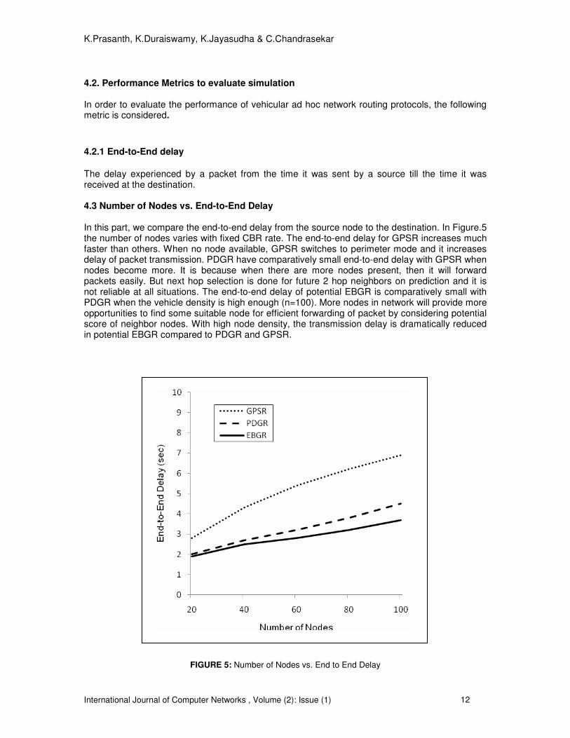
The delay experienced by a packet from the time it was sent by a source till the time it was received at the destination. 4.3 Number of Nodes vs. End-to-End Delay In this part, we compare the end-to-end delay from the source node to the destination. In Figure.5 the number of nodes varies with fixed CBR rate. The end-to-end delay for GPSR increases much faster than others. When no node available, GPSR switches to perimeter mode and it increases delay of packet transmission. PDGR have comparatively small end-to-end delay with GPSR when nodes become more. It is because when there are more nodes present, then it will forward packets easily. But next hop selection is done for future 2 hop neighbors on prediction and it is not reliable at all situations. The end-to-end delay of potential EBGR is comparatively small with PDGR when the vehicle density is high enough (n=100). More nodes in network will provide more opportunities to find some suitable node for efficient forwarding of packet by considering potential score of neighbor nodes. With high node density, the transmission delay is dramatically reduced in potential EBGR compared to PDGR and GPSR.

FIGURE 5: Number of Nodes vs. End to End Delay



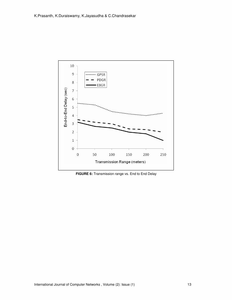
FIGURE 6: Transmission range vs. End to End Delay



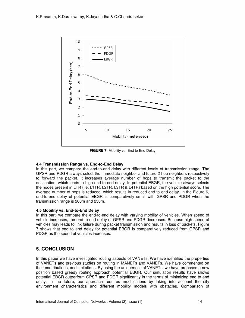
FIGURE 7: Mobility vs. End to End Delay

4.4 Transmission Range vs. End-to-End Delay In this part, we compare the end-to-end delay with different levels of transmission range. The GPSR and PDGR always select the immediate neighbor and future 2 hop neighbors respectively to forward the packet. It increases average number of hops to transmit the packet to the destination, which leads to high end to end delay. In potential EBGR, the vehicle always selects the nodes present in LTR (i.e. L1TR, L2TR, L3TR & L4TR) based on the high potential score. The average number of hops is reduced, which results in reduced end to end delay. In the Figure 6, end-to-end delay of potential EBGR is comparatively small with GPSR and PDGR when the transmission range is 200m and 250m. 4.5 Mobility vs. End-to-End Delay In this part, we compare the end-to-end delay with varying mobility of vehicles. When speed of vehicle increases, the end-to-end delay of GPSR and PDGR decreases. Because high speed of vehicles may leads to link failure during packet transmission and results in loss of packets. Figure 7 shows that end to end delay for potential EBGR is comparatively reduced from GPSR and PDGR as the speed of vehicles increases.

5. CONCLUSION In this paper we have investigated routing aspects of VANETs. We have identified the properties of VANETs and previous studies on routing in MANETs and VANETs. We have commented on their contributions, and limitations. By using the uniqueness of VANETs, we have proposed a new position based greedy routing approach potential EBGR. Our simulation results have shows potential EBGR outperform GPSR and PDGR significantly in the terms of minimizing end to end delay. In the future, our approach requires modifications by taking into account the city environment characteristics and different mobility models with obstacles. Comparison of



proposed EBGR approach with other existing approach shows that our routing algorithm is considerably better than other routing protocols in reducing end to end delay in packet transmission.

REFERENCES [1]. Charles E. Perkins and Pravin Bhagwat, “Highly dynamic destination-sequenced distance-vector

routing (DSDV),” in Proceedings of ACM SIGCOMM’94 Conference on Communications Architectures, Protocols and Applications, 1994.

[2]. T. H. Clausen and P. Jacquet. “Optimized Link State Routing (OLSR)”, RFC 3626, 2003. [3]. Richard G. Ogier , Fred L. Templin , Bhargav Bellur , and Mark G. Lewis , “Topology broadcast

based on reverse-path forwarding (tbrpf),” Internet Draft, draft-ietf-manet-tbrpf-03.txt, work in progress, November 2001.

[4]. S. R. Das, R. Castaneda, and J. Yan, “Simulation based performance evaluation of mobile, ad hoc network routing protocols,” ACM/Baltzer Mobile Networks and Applications (MONET) Journal, pp. 179–189, July 2000.

[5]. David B. Johnson and David A. Maltz, “Dynamic Source routing in ad hoc wireless networks,” in Mobile Computing, Tomasz Imielinske and Hank Korth, Eds., vol. 353. Kluwer Academic Publishers, 1996.

[6]. Vincent D. Park and M. Scott Corson, “A highly adaptive distributed routing algorithm for mobile wireless networks,” in Proceedings of IEEE INFOCOMM,1997, pp. 1405–1413.

[7]. Charles E. Perkins and Elizabeth M. Royer, “Adhoc on-demand distance vector routing,” in Proceedings of the 2nd IEEE Workshop on Mobile Computing Systems and Applications, February 1999, pp. 1405–1413.

[8]. Josh Broch , David A. Maltz , David B. Johnson , Yih-Chun Hu , and Jorjeta Jetcheva , “A performance comparison of multi-hop wireless ad hoc network routing protocols,” in Proceedings of the Fourth Annual ACM/IEEE International Conference on Mobile Computing and Networking (MobiCom ’98), Dallas, Texas, U.S.A., October 1998, pp. 85 – 97.

[9]. P. Bose, P. Morin, I. Stojmenovic, and J. Urrutia, “Routing with guaranteed delivery in ad hoc wireless networks,” in Proc. of 3rd ACM Intl. Workshop on Discrete Algorithms and Methods for Mobile Computing and Communications DIAL M99, 1999, pp. 48–55.

[10]. Brad Karp and H. T. Kung, “GPSR: Greedy perimeter stateless routing for wireless networks,” in Proceedings of the 6th Annual ACM/IEEE International Conference on Mobile Computing and Networking (MobiCom 2000), Boston, MA, U.S.A., August 2000, pp. 243–254.

[11]. Stefano Basagni, Imrich Chlamtac, Violet R. Syrotiuk, and Barry A.Woodward, “A distance routing effect algorithm for mobility (dream),” in ACM MOBICOM ’98. ACM, 1998, pp. 76 – 84.

[12]. Ljubica Blazevic , Silvia Giordano , and Jean- Yves Le Boudec , “Self-organizing wide-area routing,” in Proceedings of SCI 2000/ISAS 2000,Orlando, July 2000.

[13]. C. Lochert, H. Hartenstein, J. Tian, D. Herrmann, H. Fubler, M. Mauve: “A Routing Strategy for Vehicular Ad Hoc Networks in City Environments”, IEEE Intelligent Vehicles Symposium (IV2003).

[14]. C. Lochert, M. Mauve, H. Fler, H. Hartenstein. “Geographic Routing in City Scenarios” (poster), MobiCom. 2004, ACM SIGMOBILE Mobile Computing and Communications Review (MC2R) 9 (1), pp. 69–72, 2005.

[15]. B.-C. Seet, G. Liu, B.-S. Lee, C. H. Foh, K. J. Wong, K.-K. Lee. “A-STAR: A Mobile Ad Hoc Routing Strategy for Metropolis Vehicular Communications”, NETWORKING 2004.

[16]. H. Wu, R. Fujimoto, R. Guensler and M. Hunter. “MDDV: A Mobility-Centric Data Dissemination Algorithm for Vehicular Networks”, ACM VANET 2004.

[17]. J. Zhao and G. Cao. “VADD: Vehicle-Assisted Data Delivery in Vehicular Ad Hoc Networks”, InfoCom 2006.

[18]. Rupesh Kumar, S.V.Rao. “Directional Greedy Routing Protocol (DGRP) in Mobile Ad hoc Networks”, International Conference on Information Technology,2008.

[19]. Jiayu Gong, Cheng-Zhong Xu and James Holle. “Predictive Directional Greedy Routing in Vehicular Ad hoc Networks”, (ICDCSW’ 07).

[20]. The Network Simulator: ns2, http: //www.isi.edu/nsnam /ns/."

reducing packet transmission delay in vehicular ad hoc networks using edge node based greedy routing

Education