goodwino

1 | P a g e

Oliver Simon Wallace Goodwin

“You can’t model Marine?” - An analysis of the practical application of modelling within Marine Excess of

Loss business

The Project is submitted as part of the requirements for the award of the MSc in Risk Management and

Insurance.

August 2013

Supervisors: Chris Dickinson and Derek Atkins

2 | P a g e

Contents

Title Page Page 1

Contents

Abstract Page 3

Executive Summary Page 4

Introduction Page 6

Chapter 1: Marine Excess of Loss – Modelling History and Loss Characteristics Page 7

Chapter 2: Exposure rating Marine XL business using MBBEFD distribution Page 10

Chapter 3: Extreme Value Theory and Catastrophe Modelling Page 24

Chapter 4: Conclusions and Further Work Page 29

Appendix Page 31

Bibliography Page 39

3 | P a g e

Abstract

Marine Excess of Loss (Marine XL) modelling suffers from a lack of off-the-shelf solutions and an industry data

collection system for losses and exposures.

As a result Marine XL needs a more flexible and multi-faceted approach as a one size fits all mentality does not

capture the variety and transient nature of the original risks.

This paper, through interviews with key practitioners in the Marine XL market, practical analysis of some

standard techniques and by highlighting some published work on the subject, concludes that modelling has

value within Marine XL, as it does with all classes, but understanding the limitations as part of the process of

underwriting is extremely important.

Models do not replace underwriting but at the same time underwriters must acknowledge their value and

place in an industry and regulation of that industry which is becoming more and more model-driven.

As part of this project I have submitted some work in spreadsheet format which can be found on the enclosed

USB and on Moodle.

4 | P a g e

Executive summary

This dissertation addresses the question of what problems are faced when using, and how much value

predictive pricing models add, when pricing Marine XL business with particular focus on three classes: cargo,

hull and energy. This was done by a combination of interviewing key practitioners in the Marine XL market,

reviewing published work on the subject and using some standard modelling techniques against actual

outcomes to demonstrate their positives and limitations.

A main driver for researching and analysing this topic is to highlight the place of modelling within the bigger

picture of exposure management (RDS’s – Realistic Disaster Scenarios) for Lloyd’s Syndicates, the importance

of dialogue between actuaries and underwriters on the subject and to provide commentary on the obstacles

faced by underwriters in the class.

There has been a perceived perception in the Marine XL market that due to transient nature of the original risk

and the imperfect information associated with this quality that the use of modelling is of limited value.

Furthermore, some of the most significant losses that have been paid by reinsurers in the Marine XL market

can be categorised as non-modelled cat (catastrophe). Examples of these are the Deepwater Horizon rig

explosion and clean up in 2010, the Costa Concordia sinking and subsequent removal of wreck in 2012, the

MOL Comfort in 2013, and the Piper Alpha rig explosion in 1988.

Each of these losses highlighted the clashing nature of Marine XL catastrophes; multiple coverages being

exhausted in the same loss event, for example, physical damage, liability, hull, cargo, sue and labour, and

removal of wreck. In a market which has suffered from lack of data quality for many years, given the nature of

losses suffered, and a large non-static exposure element, modelling comes up against an obvious difficulty.

The conclusions that I have drawn by doing this research are:

1) Modelling isn’t the total answer but all models irrespective of class of business have limitations and that

using them for Marine XL involves more thought than many other lines. It is important to take this into

account in an industry which is becoming more and more model driven due to Solvency II.

2) There is going to be a most appropriate model for each class of business and an underwriter will have to

use his or her judgement to identify this. Given there are no widely accepted or off-the-shelf solutions for

Marine XL as there are in Non-Marine XL, having a more flexible and multi-faceted approach can be a

positive and a negative.

3) Actuarial input is fundamental to success in this area and there has to be a breaking down of walls of

unacceptance by underwriters. However, it is perhaps even more important to stress that modelling does

not replace underwriting nor should the decisions regarding risk appetite and general underwriting be

diluted.

4) Further work is recommended on other classes of marine business in order to validate and improve upon

the research within this dissertation. Understanding how to model and price for clashing interests or

multi-line reinsurance protections, i.e. Whole Accounts which include all classes of business as opposed to

just a mono-line such as cargo, is particularly difficult and the Marine XL market does not price adequately

for this.

5) The conclusions above should, I hope, be of interest and of use to all practitioners in the industry and

serve as a catalyst for more dialogue and solutions such as how to get more interest from commercial

modelling companies on the subject of modelling within Marine XL.

The key users I have interviewed as part of this paper are:

Richard Anson: Reinsurance buyer, Antares Syndicate 1274

Jodie Arkell: Class Underwriter, Reinsurance Group, Catlin Group

5 | P a g e

Paul Grimsey: Chief Actuary, Antares Syndicate 1274

Jun Lin: Chief Actuary, Global Re Specialty, Aon Benfield

Robert Stocker: Senior Vice President, Global Marine & Energy Specialty, Guy Carpenter

A list of the reviewed published works on the subject is listed in the bibliography of the paper.

The typical modelling techniques that I have used are the Maxwell-Boltzmann, Bose-Einstein and Fermi-Dirac

(MBBEFD) distribution class (or Swiss Re curves as they are more commonly known), Pareto Distributions and

Extreme Value Theory (EVT).

The MBBEFD are distributions derived from physics and are useful for property loss distributions. As previously

mentioned there is no widely accepted model for Marine exposures. The techniques used within MBBEFD

provide a first loss curve to describe the behaviour of a certain class of business by using an assumption of

average loss and probability of a total loss.

EVT is a branch of statistics which uses special distributions to describe extreme events. The distributions do

not describe the entire behaviour of a random variable or event; they only describe its behaviour above a

certain threshold. Essentially it is the Pareto distribution with an extra parameter.

I would like to thank all of the participants who offered their thoughts and opinions on the subject and special

thanks to Chris Dickinson, Shane Lenney and Derek Atkins for their assistance and, more importantly, patience.

6 | P a g e

Introduction

“You can’t model Marine”

Marine XL is the non-proportional protection of various classes of, for the large part, non-static marine

exposures. It has often suffered from being considered a less-sophisticated branch of reinsurance than its non-

marine counterpart due to the fact that modelling has played a lesser role historically in the pricing of business

and in the market in general. “The only major area of insurance in the UK without substantial actuarial

involvement is that referred to as MAT: Marine, Aviation and Transport.” (Czapiewski, C. 1988)

Reinsurance is structured on a layered basis and can often provide protection against a single or multiple class

or classes of Marine insurance such as Cargo, Hull and Machinery, Liability, War risks, Building risks, Port risks,

Specie, Offshore (and sometimes Onshore) energy, Yachts, Docks and Inland marine.

“Marine has always been far more difficult to model than, say, property due to the mobile nature of many of

the elements of exposure and breadth of coverage on offer.” (Anson, R. 2013)

The extent to which exposure models add value in Marine XL is an issue which divides opinion amongst market

practitioners and the heading statement is one that is used and heard often. Understanding the extent to

which predictive pricing models add value, as well as some of their limitations, is fundamental to the

underwriting process. It demonstrates a mathematical thought process and justification as well as a

representation of understanding the risk that is being considered.

Ultimately, pricing reinsurance business is both a subjective and an objective process. Assumptions are made,

exposure curves are created based on those assumptions and an output is generated giving the underwriter

some guidance as to the technical risk premium due to which he/she will apply a loading for the final premium.

“Marine business is one of the oldest areas of insurance,” (Czapiewski, C. (1998) and with this comes an

adherence to traditional methods, with which the market has sustained itself since 1688 when the Lloyd’s

market grew out of a coffee shop (Lloyd’s website).

With the advent of Solvency II the using of modelling will be a fundamental part of the business as it gives

management and analysts a justification tool and a way to best allocate and manage capital to generate a

return. “Marine isn’t viewed as the non-correlating class of business that it once was and therefore marine

accounts need to show that they can be modelled technically like their non-marine counterparts.” (Arkell, J.

2013, Personal communication)

The main purpose of this paper is to challenge and explore the idea that “You can’t model Marine” by

demonstrating some practical analysis of exposure rating a Marine Excess of Loss programme, collating the

opinions of key users and also highlighting some of the limitations that exist when using models, “it’s most

important we understand their (models’) weaknesses and limitations.” (Grimsey, P. 2013)

The reviewed literature is summarised in the bibliography of this paper. Whilst the majority of the literature is

focused on non-marine business, the statistical techniques can still be applied to marine business as the end

goal is the same; trying to predict and adequately price for the behaviour of risk that is being assumed.

7 | P a g e

Chapter 1: Marine Excess of Loss – Modelling History and Loss Characteristics

“It would seem obvious that Marine insurance covers ships. Marine implies risks arising from voyages on water

or operations linked to water, such as oil rigs. It is less clear whether peripheral risks should be included. For

example, a pipeline may be underwater and clearly a marine risk, but will come onto land at some point. It

may then still be covered by a marine insurer. Cargo, whilst on board a ship is clearly marine, but when stored

in a warehouse its nature is less obvious. Once loaded onto trucks for delivery, is it still a marine risk? Some

underwriters do cover it. Boat builders and marinas are marine risks. Marinas often have hotels and

restaurants linked to them which find their way into a Marine account.” (Working Party (1994), Marine

Insurance, General Insurance Convention, Glasgow)

The variety and transient nature of marine risks pose a challenge to reinsurance underwriters: “we mostly

have no idea where our exposures are and the value of that exposure, at any one time. However, we can

model a snapshot in time and the hope is that this snapshot is a good representation of the book of business

we are reinsuring.” (Arkell, J. 2013). Furthermore “it is important to make note of two things that exposure

bases are not. First, the exposure base is not the true exposure, which we are unable to know, both because it

is constantly changing and because it is generally a function of a large number of variables.” (Bouska, A. 1989)

This interpretation of exposure rating is true for all classes of insurance business but it seems that the data

quality in the marine classes has been particularly poor.

Historically, underwriters would rate risks by income and experience only, as there was no exposure data

available or provided. The sole technique, which is still used as part of a wider exposure capture exercise, was

to design questionnaires to identify a cedant’s exposure, both on individual, specific risks and in the aggregate

on the various classes of business written. (Lyons, G. 1988) Highlighting the major fleets, port accumulations,

country aggregates and largest energy platforms will give a reinsurance underwriter some guidance as to the

type of portfolio he/ she is reinsuring as ultimately the skill of the reinsurance underwriter is of great

importance in setting the correct rate. (Czapiewski, C. 1988)

Lloyd’s risk codes

The loss history of the Marine XL Lloyd’s risk codes further demonstrates the variety of the class as well as the

general behaviour and performance of each of the underlying risks.

A Marine XL book will typically contain a mixture of some or all of the following risk codes, with XT being the

major component part as it encompasses all classes within the same layer. This type of cover is traditionally

purchased by Lloyd’s Syndicates and the large Global Company Markets (RSA, AXA, ACE, Allianz etc.)

GX – Liability Excess of Loss TX – Hull and Machinery (incl. Building risks) Excess of Loss

VX – Cargo Excess of Loss WX – War Risks Excess of Loss (Hull)

XE – Offshore Energy Excess of Loss XT – Marine Whole Account Excess of Loss

8 | P a g e

Each one of these risks has illustrated different behaviour over the past 13 years as the below graph shows:

The two peaks shown in the graph relate to 2005 and 2010. 2005 was a very poor year for the Marine XL

market due to the large losses paid on the energy account following the Gulf of Mexico Hurricanes Katrina and

Rita. It is worth noting that both the XE and XT risk codes would have suffered due to the vertical structure of

reinsurance contracts. If, for example, a cedant purchased a 5m x 5m energy specific and then buys a 10m x

10m whole account on top, the energy loss could go through both layers which would affect both the XE

(energy specific) and XT (whole account) risk codes.

Following the hurricanes of 2005 Physical Damage cover for fixed platforms from Gulf of Mexico wind was

generally excluded from energy and whole account coverage. There were markets that did and still do write it

but a major whole account purchase would have the following typical exclusion: “Losses arising from Named

Windstorms in the Gulf of Mexico (as defined herein) emanating from the Reassured’s Upstream Energy

business.” It may, however, be possible for a cedant to have cover for liability for platforms following a Gulf of

Mexico windstorm within a whole account layer.

To highlight the volatility of the Marine XL risk codes, below is a comparison of the best and worst years (not

including 2013). This is important to show as it ties in with the assumptions and calculations behind the

exposure curves that I have created for Cargo, Hull and Energy.

If we examine the type of losses suffered by Marine XL it is clear that they are varied, often have clashing

interests and can be very severe.

9 | P a g e

Year Name of Loss Class Estimated Loss ($)

To provide assistance with exposure management, Lloyd’s provide syndicates with a set of Realistic Disaster

Scenarios (RDS) (see appendix) which map out the worst types of events that could occur and request a

syndicate’s exposure to that event. Whilst this is a prudent approach to overall risk and catastrophe

management, a recent example highlights a flaw in this methodology.

If we consider Super Storm Sandy which was a North-East U.S. windstorm which hit New York and surrounding

states in October 2012. The RDS definition of a “North-East Windstorm” is as follows:

“A North-East hurricane making landfall in New York State, including consideration of demand surge and

storm surge. The hurricane also generates significant loss in the States of New Jersey, Connecticut,

Massachusetts, Rhode Island and Pennsylvania.“ The marine loss is estimated at $0.75bn within this RDS so it

is interesting to note that when an event of this nature does occur the actual marine loss is much larger. It

highlights the importance of planning for the unknown and having an understanding that the actual exposure

and loss may differ from a prescribed scenario.

10 | P a g e

Chapter 2: Exposure rating Marine XL business using MBBEFD distribution

“Exposure rating can be a useful tool, in particular circumstances where little or no historical loss information

is available, so an experience rating approach cannot be used. It can also be combined with experience rating

into a credibility type approach to pricing a layer of X/L.” (Sanders, D. 1995)

A leading paper on the subject by Stefan Bernegger suggest that, where possible, XL treaties should be rated

using the actual exposure as opposed to just the loss experience of the past. For the purpose of rating it is

necessary to put all risks of a similar size into a risk banding and it is then assumed that all risks within the

same risk banding are homogenous.

“The correct loss distribution function for an individual band of a risk profile is hardly known in practice.” This

is why we use the distribution functions derived from large portfolios of similar risks. The exposure curves

which illustrate the distribution functions allow an underwriter to identify the necessary risk premium ratio as

a function of the excess or deductible.

The size of losses is calculated using statistical severity distributions such as the Pareto Distribution. These are

defined by their Cumulative Distribution Function (CDF) which gives the probability of observing a loss less

than or equal to some value.

The MBBEFD distribution is an alternative severity distribution as it defines the severity of the loss as a

proportion of some maximum loss. This, essentially, is the Sum Insured (SI) or a Maximum Possible Loss (MPL).

The main difference between these and the Pareto curves is the severity is measured as a percentage from 0%

to 100%. The severity distribution of the Swiss Re curves measures the probability of the size of the

proportional loss being less than or equal to some value. At a very basic level the distribution gives us a

complete description of how losses behave and the exposure curves are just another way of representing CDF.

As part of my research, I have taken 5 sets of real data for cargo, hull and energy specific reinsurance

purchases and applied the MBBEFD distribution theory to generate a price and compare this with the actual

price paid for a layer.

Independent Validation

As a starting point I used some historical actuarial data sets (see Original Cargo Data / Original Hull Data /

Original Energy Data tabs in accompanying Swiss Curves Cargo/Hull/Energy Banding spreadsheets) for each of

the three classes and compared the Swiss Re distribution with the Empirical CDF using the least squares

regression and solver.

The original actuarial data which details the Sum Insured % against the probability of the average loss being

less than or equal to some loss as a proportion of the average of all the losses for each of the three classes of

business was generated from taking a blend of the exposure data that is received at each renewal for each

class of business and creating a “typical” distribution.

In addition, I used the least squares regression, which is a standard technique to remove errors and provide a

best fit. The technique minimizes the sum of squared residuals, i.e. the difference between an actual or

observed value and the fitted value provided by some model. By using this in conjunction with solver which

minimises the total error through manipulation of the shape parameter and the probability of a total loss

percentage, it is possible to create a fitted curve.

11 | P a g e

This comparison will tell us if the Swiss Re curves are going to give a good estimate of the true price. Ultimately

the nature of the risks themselves will determine if the Swiss Re curves are suitable or not.

The data sets take an Empirical CDF against a probability percentage of observing a loss less than or equal to

the sum insured percentage of each class. If we take the cargo, for example, each 0.5% step of sum insured

results in a different probability percentage of observing a loss at this level. By comparing the MBBEFD

calculation with the data set we can imply the shape of the curve, the percentage of total loss per class and an

average loss percentage. Below are the results for each of the classes:

Cargo: Total Loss 0.137% Average Loss 1.84% Shape 0.168

Hull: Total Loss 2.015% Average Loss 5.99% Shape 3.4317

Energy: Total Loss 37.12% Average Loss 62.98% Shape 0.40652

The fitted exposure curve uses the formula =MBBEFDExposureCurve(Sum Insured %, Probability of total loss %,

Shape parameter). The screen shots for each of the classes of business are in the appendix. Furthermore, it is

possible to imply an average loss from the Probability of total loss % and the Shape parameter. This has been

done using the formula =ImplyAverageLoss(Total loss %, Shape). These three parameters are the essence of

the exposure curves.

By doing this independent validation I was able to conclude that the historical data sets were originally created

using the Swiss Re exposure curves as the fitted curves were a perfect match:

12 | P a g e

Cargo:

Hull:

Energy:

13 | P a g e

In order to fit the MBBEDF distribution all that is required is to specify the size of loss and the probability of

making a total loss (i.e. 100%). From these two parameters it is possible to create a Shape parameter and a

CDF or the probability of a experiencing a loss less than a certain percentage of the time.

By generating these curves we are able to make an assumption about their underlying severity distribution as

the shape of the curves are generated using a probability of a total loss and an implied average loss for each

class of business. Similar to the formulae used previously, to create the severity distribution curve I have used

the formula =MBBEFDDistributionFunction(Sum Insured %, Probability of a Total Loss %, Shape Parameter).

The screen shots for the severity distribution are in the appendix.

Indeed if we take this a step further we can highlight the severity distribution, using the original probability of

a total loss and average loss assumptions, in its entirety:

Cargo:

Hull:

14 | P a g e

Energy:

It is worth noting that clearly the energy curve has the highest severity whilst the cargo has the least. This ties

in with the general pattern of the Lloyd’s risk codes shown in Chapter 1 of this paper; we would expect the

severity of an energy risk to be higher as it is a more volatile class of business historically and has suffered the

largest losses.

Rather than giving us the probability of the loss being less than or equal to some value, the Swiss Re curves

give us the average loss less than or equal to some loss as a proportion of the average of all the losses. To

calculate this against a reinsurance layer we must first divide the total premiums in each of the risk bandings

mentioned earlier between the ceding company and the reinsurer. This is done by netting-down the gross

premium of the cedant so that we are left with the pure-risk premium, i.e. the premium required to cover the

predicted losses within a portfolio. For the purpose of this paper I have assumed an 80% gross loss ratio for

each portfolio meaning that to get the net income I have multiplied each gross income by 80% as, in theory,

any profit, expenses and acquisition costs should be allocated within this 20% “margin”.

Banding

The next step in the process is to divide the net premium into each of the bandings and allocate it into

premium which is retained and premium which is ceded. The loss distribution functions that have been

described above are the most commonly used way to calculate this.

To illustrate this, below is an example of a typical cargo profile, reinsurance programme and gross premium

income:

From this we can determine the bandings, the premium within each sum insured banding and the average sum

insured:

15 | P a g e

So for a 1.25m x 1.25m reinsurance layer based on a purely exposure price basis, we repeat this exercise for all

the bandings and add up pure premium using the MBBEFD distribution.

For the first banding we use 625,000 as the average, calculate the pure risk premium or net premium as 80%

of the premium in the banding and using the MBBEFD distributions for cargo business, generate the pure

premium in the layer as a function of the Limit and Deductible:

16 | P a g e

Once this was calculated I applied the same loading of 20% to generate the reinsurer’s gross price for

coverage.

In order to demonstrate the comparison of the actual rate on line (ROL) paid per layer versus the MBBEFD

output ROL, the results of the modelling exercise are shown in the tables below and on the next page.

Results

Cargo

Whilst the actual ROL paid for a layer of reinsurance may not be the correct “technical” price (there is always

going to be differentiation for preferred clients with better loss records, more benign books of business

and/or, perhaps most importantly, the role and skills of a broker), it is interesting to see how close the

MBBEFD outputs are to the actual and commercially realistic ROL’s.

The immediate conclusion that one draws from the results is that MBBEFD distributions are quite suitable for

low to middle layers (2.5 x 2.5 for Client A, 5 x 5 for Client C, 5 x 5 for Client D), poor for upper layers and the

method does not seem suitable for pricing most bottom layers. Ultimately it will depend upon the values

within a portfolio and the average sum insured within each banding.

It should be noted that using one cargo curve with one set of parameters is, in practice, too inflexible. Cargo

will behave differently depending on type, geography (i.e. if it is exposed to natural catastrophes), demand and

value.

Furthermore this approach does not take into account the actual loss history so the layers may be priced using

a burn-cost method.

17 | P a g e

Hull

The results for the hull modelling would suggest that the MBBEFD distributions do not provide a very good

method for modelling hull exposure or that the underlying assumptions for the hull curve need to be re-

evaluated. The only close match is that of Client D.

An inherent problem with using the same hull curve for each of the different portfolios is that all hull insurance

is not the same. “Standard coverage include: Hull and Machinery (H&M), Total Loss / Increased Value (IV),

Mortgagees Interests (MI), Loss of Hire (LOH), Collision Liability. But we rarely see the claims or the exposure

broken down like this.” (Tookey, L. 2006). Tookey also asks the question “how homogenous is the exposure

data and does that cause a problem?” If we are assuming a single severity distribution we have assumed that

the exposure is homogenous which may not be correct but there has to be some assumptions made and

grouping similar values together in a banding is a methodology which is widely used.

A more obvious reason why the outputs are fairly inaccurate is the 1st

excess point against the average

exposure. Clients B and C, for example, would have little exposure above their 1st

excess and as a result the

amount of applicable premium above the average risk will be smaller.

Tookey also gives us an example of where confusion may lie in a risk profile “H&M $200m, IV $50m, LOH $20m

– Maximum partial loss is $220m (H&M + LOH), - Maximum total loss is $250m (H&M + IV). In a risk profile,

this may appear as three entries (200, 50, 20), one entry of $250m or one of $270m.” This has obvious

consequences by either overstating a value or understating a clash potential for reinsurers.

Certainly a general feature of marine is the complexity of interwoven original coverages (Stocker, R. 2013).

18 | P a g e

Energy

The energy modelling outputs are fairly similar to those of the cargo, whereby, the pricing is overstated for the

bottom layers, understated for the top and seems adequate for the middle to lower layers. It is commercially

unrealistic for a cedant to pay 50%+ ROL for a bottom layer as there is no risk transfer.

If a bottom layer was clean for the past 5 years but the exposure was suggesting a very high ROL then an

underwriter may take an average of the two or weight the experience 75% to 25% exposure. Essentially the

underwriter will charge enough to cover expected losses plus a margin and if there has been no loss activity he

will use his judgement alongside market dynamics to generate a price.

Energy insurance underwent a full review following the 2005 windstorms and a significant improvement in

data presentation and software applications has become the norm. Indeed applications such as OpenXposure

and Google Earth have given energy reinsurers a clearer picture of aggregations, peak exposures and

geographical information albeit there is still an element of subjectivity to the uploading of information into

databases.

Each of the above examples demonstrates a mono-line coverage. In practice, companies buy layers of

reinsurance which cover more than one class of business. As such, “treaty excess of loss reinsurance pricing…is

one of the most complex types of reinsurance since several components need to be taken into account:

primary policy limits and deductibles, multiple lines of business covered by the same contract and loss

sensitive features that vary with the loss experience of the treaty.” (Mata, A., 2002)

19 | P a g e

Accounting for Reinstatements

“One of the common aspects of non-proportional reinsurance for some lines of business, such as catastrophe

reinsurance, is the fact that the total number of losses to be paid by the reinsurer is limited.” (Mata, A. 2000)

Reinstatement provisions allow a cedant to manage their maximum recoverable limit from a contract and they

allow a reinsurer to know the maximum aggregate he/she is exposed to during the policy period, “Usually

there is a limit in the number of losses covered by the reinsurer, where a loss is defined in the aggregate as a

layer of the same size of the maximum amount of an individual claim to the reinsurer.” (Mata, A. 2000)

An example would be a 5m x 5m layer covering hull and cargo. If the reinstatement provision was 2 @ 100%

this would mean that the cedant could recover a total of 15m during the policy period for this layer but they

would have to pay to additional premiums of 100% of the original paid for the reinstated coverage and a pro-

rata amount thereof for a partial loss. I mentioned earlier about cedants not paying for layers costing 50% +

ROL as there is no risk transfer. If we assume a 5m x 5m which costs 2.5m (50% ROL) and they have a total loss

to the layer, effectively they have paid 5m for 5m of coverage which does not constitute a very sophisticated

reinsurance buying strategy.

By using the MBBEFD assumptions previously used we can create a Monte Carlo simulation within a frequency

severity model and generate some outputs which take reinstatement provisions into account.

The below screen shot is the cargo data from Client A whose average sum insured is 5,198,020

The three metrics at the top are those carried over from the original MBBEFD exposure cargo curve. We then

apply these to the average sum insured and can estimate the average loss by simply multiplying 5,198,020 by

1.840%. The next step is to take the pure risk premium and divide this by the average loss amount. This implies

that the underlying portfolio sees approximately 73 losses (implied expected frequency of losses).

This follows the formula of E (A) = E (L). E (N) where E (A) is the expected value for the aggregate loss, E (L) is

the expected size of loss and E (N) is the expected number of losses. Calculating this information provides us

with enough information to run a frequency-severity simulation.

20 | P a g e

To simulate the losses we assume the frequency follows the Poisson distribution which will work around the

implied expected frequency shown above. For the purpose of illustration I have used 100 repetitions but in

practice you could use a lot more.

To generate some simulated reinsurance losses we need to take into account the number of losses, the

probability of a total loss, the shape, the average sum insured, the deductible and the limit. Ultimately we are

combining the frequency of the Poisson distribution with the severity described by the MBBEFD curves to give

100 simulations which is then averaged. The average of the output from this Monte Carlo simulation estimates

the average loss which is the pure risk premium that a reinsurer would charge.

To then factor in the reinstatements we extend the Monte Carlo model to generate the simulated losses as a

factor of the limit and then if these random losses are big enough to hit the reinsurance layer we can calculate

the number of limits paid, the number of reinstatements used and the total claims paid.

21 | P a g e

Here we take the simulated loss as a percentage of the limit.

Then we use an IF formula to generate the multiple limits paid from these simulated random losses.

From this it is possible to calculate the number of reinstatements utilised by the cedant over the period from

these random simulated losses.

22 | P a g e

The total claims paid number is a function of the multiple of limits paid and the actual limit.

From the simulations we can take an average of the claims paid and combine it with the average additional

premiums paid from reinstatements below:

Finally we are able to generate the pure risk premium taking into account potential reinstatements from a

number of simulations. To this we add the 20% margin to be consistent.

23 | P a g e

If we recall the actual ROL paid for this layer (28%) we can see that the generated ROL from this method is

quite high (around 43%). As mentioned previously underwriters may give credit for clean loss history and there

is no guarantee that whoever set the terms for this used the same methodology or assumptions within their

frequency-severity model. It is interesting to note that even with a relatively small average loss and probability

of total loss percentages that the output is still overstated compared to the actual price.

The Monte Carlo approach involves a few more elements than the pure exposure curves but as a result it is

more flexible which, given the characteristics of Marine XL, would bode well for a successful synergy as a

pricing tool.

The pure risk premium calculated above can be described in the following formula:

Where P is the initial premium to be charged, E(L) is the expected claim payment (average claims paid), E (R) is

the expected number of reinstatements (average additional premiums paid) and c is the proportion of the

initial premium paid for reinstatements (i.e. the number of reinstatement given in the contract).

In practice, reinstatements can be free but this will usually mean that the original up-front premium will be

that much higher and often the ROL will be above 50% ROL. Some cedants prefer to buy reinsurance this way

as they have already, in essence, paid for the reinstatement cost up front.

cRE

LEP

*)(1

)(

+=

24 | P a g e

Chapter 3: Extreme Value Theory and Catastrophe Modelling

“Catastrophe risk is fundamentally different from normal risk. It deals with events so rare that experience

doesn’t help you much predict them…you don’t know what you don’t know.” (Lewis, M. 2007)

Catastrophe Modelling is the process of using computer simulations or statistical models to assess the loss

which could occur in a catastrophic event. They are extreme events which go beyond normal occurrences such

as exceptionally high floods or exceptionally large losses and are low in frequency and high in severity.

There are two sources of CAT risks: a small number of very large claims, for example, the loss of a large oil

tanker; and infrequent external events causing many simultaneous losses such as hurricanes or earthquakes.

Natural catastrophes like hurricanes and earthquakes are modelled statistically in terms of their frequency and

severity. These elements can be combined to produce an Exceedance Probability (EP) curve of observing a

catastrophe of severity greater than some level over a time period (e.g. a year). The measure of the severity of

a catastrophe differs given the variety of catastrophes that occur; for example a storm’s severity might be

measured in terms of its maximum wind speed while an earthquake’s severity might be measured using a

shaking index.

An EP curve allows us to estimate the most severe catastrophe likely to be observed over the period to some

probabilistic confidence level.

As described by Schmutz and Doerr, rating software has been developed for many catastrophic perils and is

based on detailed data on the particular peril, which results in a very reliable risk premium for a given layer.

However, as in some cases of Marine XL, there are also perils for which there is no detailed model, either

because development is not worthwhile given the amount of business, or because the necessary data is not

available. It is my opinion, supported by nearly all the key user feedback that Marine XL suffers due to the

latter.

Where there is a lack of data, the Pareto approach is a method that can be used within EVT. “Good estimates

for the tails of loss severity distributions are essential for pricing or positioning high-excess loss layers in

reinsurance.” (McNeil, A. 1997)

EVT distributions generally measure conditional probability, rather than just probability. Conditional

probability is simply the probability of something happening given that something else has already happened.

Some lines of business, Marine XL in particular, can experience exceptionally large losses which are low in

frequency making the existing loss data is often very limited in scope. Furthermore, where the claims patterns

are irregular, such as in Energy (slide 45 of IUMI presentation in San Diego, 2012) and claims reserves are set

according to knowledge about individual claims, it can prove to be very challenging to set the correct

premium.

Future catastrophic losses have the potential to be far greater than the losses already observed and EVT can

be used to extrapolate the existing loss data to find out how large future catastrophic losses could be and their

probabilities. To estimate the EVT distribution, a threshold (u) above which the tail is fitted, must be set.

Values above this threshold represent large claims which are low in frequency but high in severity and are

commonly called Atypical claims. Values below this threshold are high frequency and low severity and are

commonly called Attritional claims.

Pareto Distribution

EVT is essentially the Pareto distribution with an extra parameter. The only real difference is its necessary to

have the necessary data to fit the distribution to the risk.

25 | P a g e

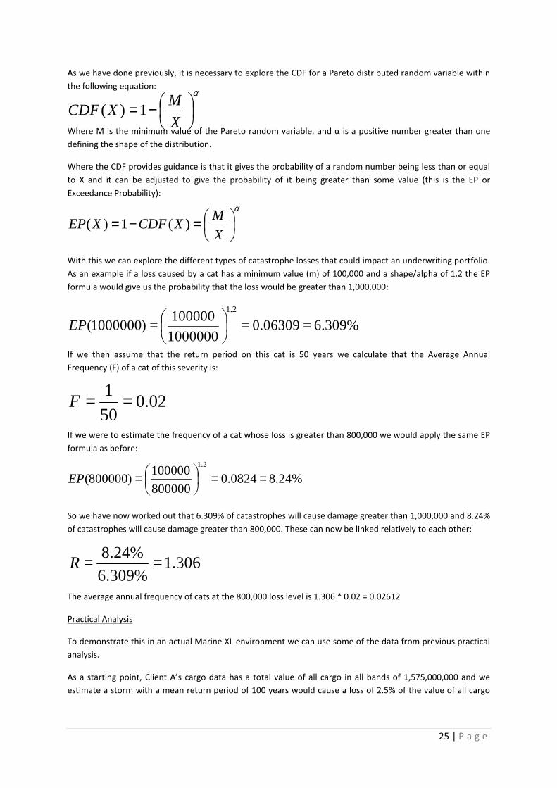
As we have done previously, it is necessary to explore the CDF for a Pareto distributed random variable within

the following equation:

Where M is the minimum value of the Pareto random variable, and α is a positive number greater than one

defining the shape of the distribution.

Where the CDF provides guidance is that it gives the probability of a random number being less than or equal

to X and it can be adjusted to give the probability of it being greater than some value (this is the EP or

Exceedance Probability):

With this we can explore the different types of catastrophe losses that could impact an underwriting portfolio.

As an example if a loss caused by a cat has a minimum value (m) of 100,000 and a shape/alpha of 1.2 the EP

formula would give us the probability that the loss would be greater than 1,000,000:

If we then assume that the return period on this cat is 50 years we calculate that the Average Annual

Frequency (F) of a cat of this severity is:

If we were to estimate the frequency of a cat whose loss is greater than 800,000 we would apply the same EP

formula as before:

So we have now worked out that 6.309% of catastrophes will cause damage greater than 1,000,000 and 8.24%

of catastrophes will cause damage greater than 800,000. These can now be linked relatively to each other:

The average annual frequency of cats at the 800,000 loss level is 1.306 * 0.02 = 0.02612

Practical Analysis

To demonstrate this in an actual Marine XL environment we can use some of the data from previous practical

analysis.

As a starting point, Client A’s cargo data has a total value of all cargo in all bands of 1,575,000,000 and we

estimate a storm with a mean return period of 100 years would cause a loss of 2.5% of the value of all cargo

α

−=X

MXCDF 1)(

α

=−=X

MXCDFXEP )(1)(

%309.606309.01000000

100000)1000000(

2.1

==

=EP

02.050

1 ==F

%24.80824.0800000

100000)800000(

2.1

==

=EP

306.1%309.6

%24.8 ==R

26 | P a g e

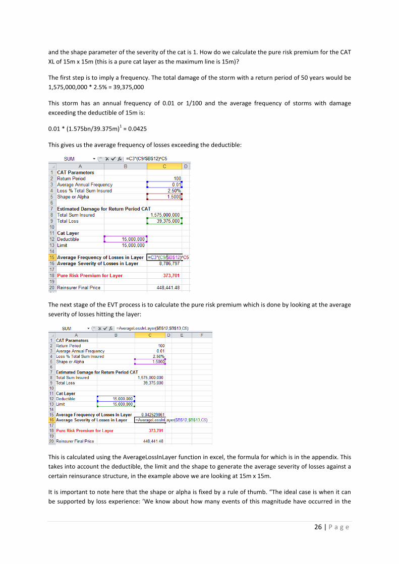
and the shape parameter of the severity of the cat is 1. How do we calculate the pure risk premium for the CAT

XL of 15m x 15m (this is a pure cat layer as the maximum line is 15m)?

The first step is to imply a frequency. The total damage of the storm with a return period of 50 years would be

1,575,000,000 * 2.5% = 39,375,000

This storm has an annual frequency of 0.01 or 1/100 and the average frequency of storms with damage

exceeding the deductible of 15m is:

0.01 * (1.575bn/39.375m)1 = 0.0425

This gives us the average frequency of losses exceeding the deductible:

The next stage of the EVT process is to calculate the pure risk premium which is done by looking at the average

severity of losses hitting the layer:

This is calculated using the AverageLossInLayer function in excel, the formula for which is in the appendix. This

takes into account the deductible, the limit and the shape to generate the average severity of losses against a

certain reinsurance structure, in the example above we are looking at 15m x 15m.

It is important to note here that the shape or alpha is fixed by a rule of thumb. “The ideal case is when it can

be supported by loss experience: ’We know about how many events of this magnitude have occurred in the

27 | P a g e

last 20 years.’ The observation point is expressed as a percentage of the total sums insured so that it can be

adjusted to a portfolio of any size.” (Schmutz, M. and Doerr, R. (1998)

Given the maximum line of 15m in this example I have suggested that a 2.5% of total sum insured will be lost

in a 100 year event. This generates a total loss of roughly $40m which is just over 2.5 times the maximum line.

This could quite feasibly occur in a large catastrophe event.

By combining the average frequency and average severity we can calculate the pure risk premium before

applying the same load as before (20%).

The actual ROL in this instance was 3% compared with a generated ROL of 2.99%. In order to get to this figure I

have worked backwards to see what type of alpha would have been applied to this type of event in order to

get roughly 3% ROL as a price. By doing this it is possible to create a database of different scenarios which can

be used for future pricing and gives some flexibility to an underwriter.

The cargo example above has been used without any prior knowledge of cat losses for that specific account. It

is interesting to see the outcome for the other classes where some loss information is available.

If we take a hull example of 7.5m x 17.5m and we know that this portfolio suffered a Sandy loss of 22.222m we

are able to use this as a loss % of the total sum insured:

28 | P a g e

This example provides us with a look at what the alpha would be for that amount of damage required on that

value of portfolio, assuming of course that the actual price charged of 8.5% is the absolute correct technical

price, which it is unlikely to be due to the amount of variants and confidentiality surrounding leader pricing

methodology.

I have also taken an example from an energy portfolio which demonstrates a hurricane IKE type loss. It is

important to bear in mind that this type of loss is unlikely to happen again on this type of portfolio due to the

more restrictive reinsurance cover for Gulf of Mexico wind damage to fixed platforms as mentioned in Chapter

1.

Similar to the hull scenario, I have had to assume an alpha that generates a loss of 100m given the actual loss

suffered from IKE. Again, there are limitations to this method but it does give an underwriter an idea of what

to expect from this type of scenario and provide flexibility if the portfolio changes size or the reinsurance

structure changes.

Taking events like Sandy or IKE makes sense theoretically but it does leave an issue with estimating the mean

return period for these events. This does leave the “rule of thumb” methodology open to interpretation and

again speaks volumes about the lack of off-the-shelf solutions available to Marine XL underwriters.

“Cat charges – The trickiest element of our model is pricing the cat element of the risk. Currently we use RMS

for static storage and when we have the information and outside of that we add a cat load in line with what

the non-marine team would do. It’s not an ideal method for modelling cat and I think the marine market is bad

at pricing for cat in general. Super Storm Sandy is a good example of this.” (Arkell, J. 2013)

“As a rule, when the insurance sector turns its attention to accumulation losses, property insurance takes

centre stage. Major natural catastrophes in recent years have heightened risk managers’ awareness of the fact

that extremely high losses can accumulate here in the worst case. In the special line of marine insurance, on

the other hand, the problem of accumulation continues to receive far too little attention.” (Munich Re, 2013)

29 | P a g e

Chapter 4: Conclusions and Further Studies

A significant contribution to this paper has been the opinions of key practitioners in the Marine XL industry:

brokers, reinsurance buyers, actuaries and underwriters. Whilst opinions will vary on the topic, by accessing

this experience across a broad spectrum of key users, I feel that I have accurately represented the class of

business opinion in respect of modelling.

A copy of the completed questionnaires is enclosed in the Appendix and as part of a conclusion it is prudent to

draw on some of the main points. Clearly the non-static element of marine risks makes the role of modelling,

at times, limited. We cannot say with any confidence what our exact exposure is and the value of that

exposure at any one time. Where models can add value is they look at a snapshot in time of information and

underwriters will trust that this snapshot is a good representation of the book of business being reinsured.

Whilst Marine has its own unique obstacles to overcome when modelling (which is the case for most

commercial lines of business), this should not put people off using them. “I don’t want people to get overly

reliant on models because that can be very, very dangerous…you don’t want people to let the models do the

thinking for them. We need to balance it out with models to inform and humans to take that information and

do the right thing with them.” http://www.insurancejournal.tv/videos/7801/

The use of modelling within the class has been a fairly recent phenomenon (in the last 15 years) but the lack of

“off the shelf” modelling solutions for marine business makes modelling certain elements rather tricky and

often the issue is a lack of usable data and where data is available, there is often a question surrounding

allocation of cost to collate, cleanse and verify this data.

Data is key to establishing an accurate and acceptable exposure rating method and “in the absence of

adequate data, benchmark severity distributions fitted to industry wide data by line of business might be

used.” (Mata, A., 2002). However data collected is also threatened by changes in frequency and severity, which

have arisen due to changes to underlying exposure, for instance in the energy industry where values have

recently increased or by regulatory factors where governments change regulations to increase liability

exposures. (Stocker, R. 2013)

“Data is such a fundamental, important thing for predictive modelling that it can’t be underestimated how

crucial it is and potentially how time consuming and costly it could be to get good appropriate data to be able

to do the predictive modelling you want….80% of it is data and 20% of it is validation. We focus a lot on the

modelling effort but the data is absolutely significant and requires a lot of thought and a lot of care, a lot of

time and, in some ways, a lot of money.” http://www.insurancejournal.tv/videos/7801/

The use of exposure modelling, from which a lot of pricing models are derived, does not guarantee accuracy

and surprises are always going to present themselves. An example would be in the Non-Marine XL market

which is heavily reliant on industry models such as RMS / AIR etc. Conceptually CAT models make sense but

their accuracy in some cases has been poor, for example the largest insurance losses predicted by CAT models

for Hurricane Katrina were $25bn; the post event estimates are closer to $43bn. It is true that CAT models can

suffer from Model Risk whereby there are too many elements to it so one of my concluding points is that a

good model is a simple model which can be easily understood and used.

Underwriters in the class need to have flexibility to choose which model they use as well as being able to

disagree with the outcome as ultimately “models don’t replace having a pricing strategy or having a claims

management strategy…it’s a tool and it gives you a very useful bit of information and you still have to make

prudent decisions about what to do with that information.” http://www.insurancejournal.tv/videos/7801/

It is for this reason that a strong dialogue between actuaries and underwriters is paramount as well as taking

into account a multi-faceted approach for Marine XL “with so many moving parts marine needs a more flexible

and multi-faceted approach. Ironically given the general perception that marine lags behind non-marine I

30 | P a g e

think this requirement will ultimately produce a better model than one founded on an over reliance on

computer cat models.” (Stocker, R. 2013).

This point is particularly prevalent when considering the RDS returns and part of the larger exposure

management landscape. A cargo portfolio is generally international in its composition. This means that it is

inherently exposed to several RDS scenarios (California Earthquake, Japanese Earthquake, European

Windstorm and Marine Collision scenarios). How do you price for all of these events? Furthermore, how do

you know at any one time what cargo is where and what the value of that cargo is?

The fact that the largest losses to hit the Marine XL market in the last 5 years would be considered as non-

modelled cats suggests that there is still a lot of work to be done understanding the original nature of the risk

being considered by modelling companies and the underwriting community in general.

In an article entitled “In Nature’s Casino”, Michael Lewis analyses the history and application of catastrophe

modelling with a focus on Hurricane Andrew in 1992 and Hurricane Katrina in 2005. He makes particular

reference to Karen Clark, the founder of Applied Insurance Research (A.I.R.) and the predictions that she made

following Hurricane Andrew: “Back in 1985…Clark wrote a paper with the unpromising title ‘A Formal

Approach to Catastrophe Risk Assessment in Management.’ In it, she made the simple point that insurance

companies had no idea how much money they might lose in a single storm…The insurance industry had been

oblivious to the trends and continued to price catastrophic risk just as it always had, by the seat of its pants.”

In order to better assess the potential cost of catastrophe, Clark collected long-term historical data on

hurricanes and combined it with modern property exposure data. She was able to create a powerful tool, both

for judging the probability of a hurricane hitting one particular area and for predicting the loss cost it may

inflict. One of the most alarming predictions was the Miami hurricane of 1926, which she predicted would

cause $60bn-$100bn of property damage if it were to happen in the present-day. Unfortunately for Clark, she

was presenting this information to a room full of Lloyd’s underwriters who has made fortunes of the past 20

years insuring against hurricanes. “But – and this was her real point – there hadn’t been any catastrophic

storms! The insurers hadn’t been smart. They had been lucky.”

As further work on the subject I suggest that some analysis on multi-line coverages is done as well as

generating models that go further than just an RDS specific scenario, as feasibly a reinsurance portfolio can

suffer other types of losses. A good example of this is the Sandy loss itself and the MOL comfort incident which

happened this year.

In terms of modelling Marine XL it is important to be cognisant of all methods of pricing, as ultimately the

“correct” rate is one that is accepted by the supply and demand dynamics of the market. Furthermore “If both

exposure and experience rates have been successfully estimated and they differ, then there is a clear question

of which to use. If the book has changed dramatically over a period of time, then experience rating will be

meaningless. If the future exposure is likely to have changed, then the exposure rate is in doubt. In practice the

rate lies between the two.” (Sanders, D. 1995)

Both EVT and MBBEFD can be used to model Marine but I think a variety of curves is required for different

types of cargo, geography and value and other loss characteristics. “Both work relatively well for working to

mid layers. For high (risk exposed) layers, MBBEFD will work better when limited experiences are available. For

clash and whole account layers, both work poorly. “(Lin, J. 2013)

As part of further studies on the subject I think that a comparative study with pure Pareto methodology should

be analysed. “We find that pareto curves come out with sensible results for low level risk layers, sensible

results for top risk layers, generally too penal on middle layers and too generous on cat/clash layers.” (Arkell, J.

2013)

31 | P a g e

The use of models will undoubtedly increase in the next few years and it is fundamental that we can have a

level of confidence in the outputs but it is important that we don’t lose sight of what the business is all about:

risk and reward. Models can greatly assist in improving understanding of this: “One positive side effect of this

heightened risk awareness is that it can create an incentive to develop new risk models or adapt established

risk models from property insurance to meet the needs of marine insurance.” (Munich Re, 2013)

32 | P a g e

Appendix

Screen shots of Swiss Curves Cargo Banding

Methodology to create Exposure Curve

Underlying Severity Distribution

Screen shots of Swiss Curves Hull Banding


33 | P a g e


Screen shots of Swiss Curves Energy Banding



Interview Transcripts with Key Users:

Richard Anson

1) “You can’t model Marine” – to what extent do you agree with this statement?

Marine has always been far more difficult to model than, say, property due to the mobile nature of many

of the elements of exposure and the breadth of coverage on offer.

2) Modelling has only been widely used in marine in last 15 years – why is that?

Undoubtedly this has been driven by the advent of computers and the internet which has enhanced our

ability to capture the nuances of the marine product (location and coverage). The expansion of data

creates the opportunity to identify the key drivers of exposure which can then be applied to portfolio data

on a predictive basis.

3) What are some of the issues with the current models?

34 | P a g e

The marine market has a tendency to under-estimate (and to therefore under-price) exposure to natural

perils. Exposure curves are often based on a data set which is too small to give a robust rating model.

4) Does the industry have sufficient usable data to create accurate models?

In respect of a limited number of perils only.

5) Do we do enough as an industry to share and standardise data?

Could do more….

6) What is your experience of using MBBEFD curves and EVT for Marine XL pricing?

None at present. My pricing for marine classes is based on extrapolating past losses via pareto.

7) Do the distributions differentiate well enough between the classes?

8) What part do you see models playing over next 10 years in our market?

Ever increasing as the data available to parameterise the models increases.

Jodie Arkell


Agree to some extent and the main reason for this is that in the marine world we mostly have no idea where

our exposures are and the value of that exposure, at any one time.

However, we can model a snapshot in time and the hope is that this snapshot is a good representation of the

book of business we are reinsuring.

There are many marine classes that can be modelled using non-marine models, such as static storage in

regards to cargo, inland marine, onshore and offshore energy….think that’s about it.


Unlike non-marine there isn’t an off the shelf solution (that I know of) for marine business.

Also, in the past the quality of data received was terrible and has improved vastly. Previously, underwriters

rated risks using income and experience, no exposure data or very little was provided. Believe there has been a

market push for much more detailed information and data, but we are still way behind the non-marine

market.


Lack of flexibility – models are built with a “one size fits all” mentality but risks are rarely the same in the

marine world. Every risk differs from the make-up of the risks to the location. I think it’s difficult to allow for all

the variances but more flexibility needs to be incorporated.

Snapshot in time – models are based on information at a point in time.

Cat charges – The trickiest element of our model is pricing the cat element of the risk. With the curves and

data we have, I am confident that the risk rating in our model is very good. The cat is a different story.

Currently we use RMS for static storage and when we have the information and outside of that we add a cat

load in line with what the non-marine team would do. It’s not an ideal method for modelling cat and I think the

marine market is bad at pricing for cat in general. Super Storm Sandy is a good example of this.

Clash – another difficult element to price for and can be forgotten about. When writing a marine account how

do you price for the 2 hulls colliding of which one insured could be on both or a cargo vessel sinking and one

insured writing both the hull and cargo (MOL Comfort!). You would like to think that clients manage their

accumulations but this isn’t always possible (a reason for buying reinsurance). Reinsurers must make sure they

are applying a charge for this but difficult to quantify.

35 | P a g e

Overall I think there are inherent problems with all models and marine models are no different to this, as long

as the underwriter is aware of the weaknesses and uses the model as a tool rather than the answer then they

can be very useful.


Possibly but the data needs cleansing, I know from our point of view the integrity of some of the data is

questionable but it’s all we have and view it as better than nothing.


No. Everyone has different models and therefore needs the data in different formats. Again I believe this is

down to the lack of off the shelf solutions.


We use Pareto curves, not sure if these are the same kind of thing! We find that pareto curves come out with

sensible results for low level risk layers, sensible results for top risk layers, generally too penal on middle layers

and too generous on cat/clash layers.


Yes. I believe so. We write a multifaceted account and have 13 curves, most of which are very different.


It’s inevitable that we are going to use modelling more and more in our business. Management and analysts

like models!!!

(Re)Insurance companies want to get the best return on capital. Since marine is exposed to nat cats, the

marine underwriters are competing with the non-marine underwriters for aggregates, internally. Marine isn’t

viewed as the non-correlating class of business that it was once viewed as and therefore marine accounts need

to show that they can be modelled technically like their non-marine counterparts. Even though in the past the

models in the non-marine world have been generally wrong but in my experience, management would much

prefer to look to models than other methods.

Also believe that there will be a bit of a shortest our experience in the marine world as the older generation

retire there is a shortage of those people in the next generation. Could mean a reliance on models rather than

traditional underwriting techniques….!

Jun Lin


It depends. For normal risk losses, the general statistical method, be it experience or exposure rating, should

work well.

The clash and Nat Cat losses, I will agree to a certain extent. Having said that, the difficulty around modelling

clash losses is not unique to Marine. Scenario like WTC, I am not sure anyone can be confident to say they

know how to model it.

Nat Cat is difficult as most models are designed for property where the value, location, and the physical

aspect of the items are relatively well understood. (again only for peak risk areas like US wind/EU wind etc.

Thailand/New Zealand EQ/Chile EQ will tell you a different story) It is less of a problem for static storage risks

36 | P a g e

where value and location are known, though the vulnerabilities are poorly matched as models are not

developed for cargos.


Quality of data is the main issue. As data quality improve, it is getting more confident to model marine.


how long do you have?!

vulnerability is the main issues. models are made for property risks where the physicalities are very different

to cargo, floating objects.

Generally the water/wave impacts from a nat cat events are less well understood. Even for property, the

confidence on the modelled results on flood particularly flood following wind and storm surge is not that high.

Sandy is a good example where model miss for property is relatively high given the size of the event.

The other main issue is the value and location of the goods in transit.


No.


Depends. In some areas like platforms and big risks, the quality has got better in the last few years.


Both works relatively well for working to mid layers. For high (risk exposed) layers, MBBEFD will work better

when limited experiences are available. For clash and whole account layers, both work poorly.


Yes. Not sure where you are going with this, as it is kind of obvious.


Whether we have confidence in the figures, model will be increasingly required by investors, regulators

Paul Grimsey


Strongly disagree. I agree Marine has its unique obstacles to overcome when modelling (as do most

commercial lines classes of business) – it just requires a little more thought. We should not try to have one

model that fits all classes, rather individual models designed with the class of business in mind.


- The rise of the actuary!

- Data quality (both systems and volumes)

- (Partial) acceptance by the underwriting community

- Regulation / SII (at least in part)


- People believe they are 100% accurate without really understanding limitations / modelling

assumptions

37 | P a g e

- Sometimes overly complex for the sake of it

- Generally poorly understood


Yes. We need to make allowances for scarcity of data, but it’s lazy to just say there’s not enough data so

there’s nothing we can do.


LMA triangles and RAA data are 2 examples that we use here. Issues are always going to be commercial

sensitivity, and time lags because of delays in collection. I can’t see any real drivers for this to change.


We use parts of EVT in our CK parameterisation, but as things stand no direct link to Marine XL pricing.


I think parameterised properly we have enough distributions available to us. Key focus for goodness of fit is

different when considering CK vs pricing vs reserving.


SII forces us to use models. However it should always be a tool to support a decision, rather than blindly doing

what the models tell us with no extra thought.

Models will be fundamental to the business – it’s most important we understand their weaknesses and

limitations.

Robert Stocker

1) You can't model marine.

Only difference in modelling standard between marine and non-marine capability is that there are widely

accepted cat models for property exposures. That difference is overstated in several ways. Firstly some

marine exposures are covered by existing cat models. Secondly the property cat models are neither 100%

credible or provide 100% coverage. Lastly catastrophe exposures are not the sole pricing factor; other

elements are equally significant and can be accurately considered without such models.


A systemic approach to pricing has been used for longer than 15 years. Linking that approach to broader

considerations (a fully linked up DFA model for instance) you are correct is a more recent development.

However that change is not limited to marine, it applies to all areas of insurance and reinsurance.


I would like to split this into two parts highlighting key issues, namely marine catastrophe modelling and

secondly the main body of actuary supported pricing.

Marine catastrophe modelling

There are problems with exposure capture in that many of the exposures move, but that issue applies to all

pricing matters. There are also weaknesses in the approach taken by the modelling firms in trying to transpose

property building codes and damage factors to marine exposures. Even where some effort has been made for

38 | P a g e

instance on GoM energy the results have been questionable undermined partly by the factors above but also

by other feature of marine such as the complexity of interwoven original coverage’s. All of the issues

mentioned and other issues no mentioned could be tackled with sufficient money. However in simple terms

the industry and ultimately the consumers are not willing to pay that money for more accurate catastrophe

models.

General pricing modelling

The details of actuarial techniques applied to marine I presume are the same as those applied to other areas of

reinsurance and so are not worthy of specific comment. The main issue specific to marine is that there is no

industry data collection system; no-one collates loss and exposure data for the industry as for instance PCS

does. As a result even the biggest reinsurer’s data set is compromised as it merely reflects the experience of

that reinsurer’s portfolio. Where (laudable) attempts have been made to collect data such as those for energy

insurance the data set is also limited and compromised for instance, by a lack of underlying value data.

The data collected is also threatened by changes to frequency and severity. These have arisen due to changes

to underlying exposure, for instance in the energy industry where values have recently increased or by

regulatory factors where for instance governments change regulations to increase liability exposures. These

factors must however be familiar from other industry segments so hopefully the actuaries can adjust their

models accordingly.


See answer 3 for data collection issues, but main point is who might pay for any industry approach.


Standardisation should be possible and the basis for it is in place in a number of areas for instance Clarkson

numbers for identifying vessels and rigs. Sharing data if it is collated is problematic due to cost issues.


My direct experience is limited as normally only see outputs rather than mechanics.



The role of models will increase over the next ten years. However I cannot see attaining total dominance over

the underwriting process as may be the case in monoline segments of the industry. With so many moving

parts (excuse the pun) I think marine needs a more flexible and multi-faceted approach. Ironically given the

general perception that marine lags behind non-marine I think this requirement will ultimately produce a

better model than one founded on an over reliance on computer cat models.

Formula used

MBBEFDDistributionFunction

The Equation for the CDF for the MBBEFD Distribution is:

).1().1(

11

1 bgbg

bx −+−−− −

39 | P a g e

Where b is the shape parameter and g is the reciprocal of the probability of total loss (ie 1 / Probability of total

loss).

In the spreadsheet this is implemented in the MBBEFDDistributionFunction and gives the probability of a loss

being less than or equal to some proportional loss of the sum insured (X).

MBBEFDExposureCurve

The formula for the Exposure curve used in pricing of layers is:

Where b is the shape parameter and g is the reciprocal of the probability of total loss (ie 1 / Probability of total

loss).

In the Spread sheet this is implemented in the MBBEFDExposureCurve and proportion of the expected loss

below a value x

MBBEFDParameter

It is possible to calculate the Shape parameter (b) from the probability of the total loss (p) and the average loss

(m) using the following formula:

To find b (or the shape) given g (which is 1/p) and m this equation has to be solved iteratively since it cannot

be inverted algebraically

MBBEFDParameter function solves this equation iteratively using the bracketing algorithm.

AverageLossInLayer

Based on the density of the underlying Pareto Distribution we can calculate this average severity S as the

following integral:

Solving this integral we obtain the following formula for the average loss in the layer:

There is a special case for this formula when a is equal to 1:

Formulae provided by Chris Dickinson

( ) ( )( )bgbgbg

bgbx .1.1)..ln(

).1).(ln(1 −+−−

−

).1).(ln(

)1).(.ln(

bgb

bbgm

−−=

( ) dxxDLdxxDDxSDL

DL

D

........ 11 −−∞

+

−−+

∫∫ +−= αααα αα

−

+−

=−

11

1 α

α D

DLDS

+=D

DLDS ln.

40 | P a g e

Bibliography

Bernegger, S. (2005) The Swiss Re Exposure Curves and the MBBEFD Distribution Class, Astin Bulletin (2005)

Volume: 27, Issue: 1, Pages: 99–112

Bouska, A. (1989) Exposure Bases Revisited

Czapiewski, C. (1988), chairman of working party: Marine Insurance and Reinsurance, 1988 General Insurance

Convention

Farr. D. (2012) Global Statistics from the International Union of Marine Insurance Facts and Figures Committee,

GIRO Conference and Exhibition, San Diego 2012

Lewis, M. (2007), In Nature’s Casino, The New York Times

Lyons, G. (1988), chairman of working party: L.M.X. – Excess of Loss Reinsurance of Lloyd’s Syndicates and

London Market Companies, 1998 General Insurance Convention

Malde, S. (1994), chairman of working party: Marine Insurance, 1994 General Insurance Convention

Mata, A., Fannin, B. and Verheyen, M. (2002) Pricing Excess of Loss Treaty with Loss Sensitive Features: An

Exposure Rating Approach

Mata, A. (2002) Pricing Excess of Loss Reinsurance with Reinstatements, Astin Bulletin, Vol. 30, No. 2, 2000,

pp.349-368

McNeil, A. (1997) Estimating the Tails of Loss Severity Distributions Using Extreme Value Theory

Munich Re Publication: “Topics Magazine” – Issue 1/2013 Page 6 – “Avoiding accumulation risks”

Sanders, D. (1995), chairman of working party: Pricing in the London Market, 1995 General Insurance

Convention

Sanders, D. (1996), chairman of working party: Pricing in the London Market: Part 2, 1996 General Insurance

Convention

Schmutz, M. and Doerr, R. (1998) The Pareto model in property reinsurance: Formulas and applications

Tookey, L. (2006), Marine Reinsurance, CARe 2006

http://www.insurancejournal.tv/videos/7801/ “Insurance Journals Podcast” – Insurance Journal's Andy

Simpson continues the discussion on predictive modeling with two actuaries, Claudine Modlin, a senior

consultant with Towers Watson, and Steve Armstrong, who is chief pricing actuary for Chartis Consumer

Insurance

Piper Alpha 25 Years On:

http://www.lloyds.com/~/media/Images/Newsletter/Events/UK%20Events/FINAL%20VERSION%202%20%20Pi

per%20Alpha%20Slides%20Lloydscom.pdf

Realistic Disaster Scenarios: Scenario Specification January 2013

http://www.lloyds.com/~/media/Files/The%20Market/Tools%20and%20resources/Exposure%20management

/RDS_Scenario_Specification_January_2013.pdf

41 | P a g e

Spreadsheets:

EVT Pareto

Loss Summary

Lloyds Risk Codes since 2000

Modelling Results

Monte Carlo Example

Swiss Curves Cargo Banding

Swiss Curves Energy Banding

Swiss Curves Hull Banding

goodwino

Documents