WORKING PAPER NO 164

GLOBAL INTEGRATION OF INDIA’S MONEY MARKET:

INTEREST RATE PARITY IN INDIA

Vipul Bhatt Arvind Virmani

JULY 2005

INDIAN COUNCIL FOR RESEARCH ON INTERNATIONAL ECONOMIC RELATIONS

Core-6A, 4th Floor, India Habitat Centre, Lodi Road, New Delhi-110 003 Website: www.icrier.org

GLOBAL INTEGRATION OF INDIA’S MONEY MARKET:

INTEREST RATE PARITY IN INDIA

Vipul Bhatt Arvind Virmani

JULY 2005

The views expressed in the ICRIER Working Paper Series are those of the author(s) and do not necessarily reflect those of the Indian Council for Research on International Economic Relations (ICRIER).

CONTENTS

Page No

FOREWORD I

1 INTRODUCTION 1

2 LITERATURE REVIEW 2

3 MODEL AND ESTIMATION 4

3.1 Estimating Equations 4

3.2 Econometrics 6

3.3 Data Sources 7

4 RESULTS 9

4.1 Stationarity and Co-integration 9

4.2 Covered Interest Parity 10

4.3 Un-covered Interest Parity 11

4.4 Exchange Risk and RBI Intervention 12

5 CONCLUSIONS 13

6 REFERENCES 15

7 APPENDIX: TESTS 17

7.1 Order of integration 17 7.1.1 Sequential ADF Test for unit root 17 7.1.2 Phillips-Perron Test 18

7.2 Test for Co-integration: Johansen’s Methodology 18

7.3 Call Money Assymmetry 19

TABLES

Table 1 : Unit Root Test Results................................................................................................ 9 Table 2: Results of Johansen’s Co-integration Test................................................................ 10

FIGURE

Figure 1: 3-Month Forward Premium (F) and India-US Interest Differential (Idiff) 8

i

Foreword

Financial openness exists when residents of one country are able to trade

assets with residents of another country, i.e. when financial assets are traded goods. A weak definition of complete financial openness, which one might refer to as financial integration, can be given as a situation in which the law of one price holds for financial assets- i.e. domestic and foreign residents trade identical assets at the same price. A strong definition would add to this the restriction that identically defined assets e.g. a six-month Treasury bill, issued in different political jurisdictions and denominated in different currencies are perfect substitutes in all private portfolios. The degree of financial integration has important macroeconomic implications in terms of the effectiveness of fiscal and monetary policy in influencing aggregate demand as well as the scope for promoting investment in an economy.

The paper shows that the short-term (up to 3 month) money markets in India are getting progressively integrated with those in the USA even though the degree of integration is far from perfect. Covered interest parity is found to hold for while uncovered interest parity fails to hold. The difference between the two can be attributed to the existence of an exchange risk premium over and above the expected depreciation of the currency. Analysis of RBI interventions in response to foreign exchange shocks suggests that these may play a role in the deviations from interest parity. Further work needs to be done however on this as well as on instruments of other maturity such as 1 month and 6 month (for which consistent data was not available).

Arvind Virmani

Director & Chief Executive ICRIER

July 2005

1

1 INTRODUCTION

Financial openness exists when residents of one country are able to trade

assets with residents of another country, i.e. when financial assets are traded goods. A

weak definition of complete financial openness, which one might refer to as financial

integration, can be given as a situation in which the law of one price holds for

financial assets- i.e. domestic and foreign residents trade identical assets at the same

price. A strong definition would add to this the restriction that identically defined

assets e.g. a six-month Treasury bill, issued in different political jurisdictions and

denominated in different currencies are perfect substitutes in all private portfolios.

The degree of financial integration has important macroeconomic implications in

terms of the effectiveness of fiscal and monetary policy in influencing aggregate

demand as well as the scope for promoting investment in an economy.

The free and unrestricted flow of capital in and out of countries and the ever-

increasing integration of world capital markets can be attributed to the process of

Globalization. The benefits of such integration are liquidity enhancement on one hand

and risk diversification on the other, both of which are instrumental in making

markets more efficient and also facilitate smooth transfers of funds between lenders

and borrowers. India began a very gradual and selective opening of the domestic

capital markets to foreign residents, including non-resident Indians (NRIs), in the

eighties. The capital market opening picked up pace during the nineties. In this paper

we try and estimate the degree of financial integration between India and the rest of

the World, by focussing on the degree of integration of the Indian money market with

global markets.

Frenkel (1992) in his review of Capital Mobility measurement outlined four

different definitions of perfect capital mobility that are in widespread use, of which

three are of relevance to the current paper. These are real interest parity, uncovered

interest parity and covered interest parity. (i) Real interest parity hypothesis states

that international capital flows equalise real interest rates across countries. (ii)

Uncovered interest parity states that capital flows equalise expected rates of return on

countries’ bonds regardless of exposure to exchange risk. (iii) Covered interest parity

states that capital flows equalise interest rates across countries when contracted in the

same currency. Frenkel (1992) shows that these three definitions are in ascending

order of specificity in the following sense. Only definition (iii) that the covered

2

interest differential is zero is an unalloyed criterion for “capital mobility” in the sense

of the degree of financial market integration across national boundaries. Condition

(ii) that the uncovered interest differential is zero requires that (iii) hold and that there

be zero exchange risk premium. Condition (i) that the real interest differential be zero

requires condition (ii) and in addition that expected real depreciation is zero.

2 LITERATURE REVIEW

The uncovered interest parity (UIP) theory states that differences between

interest rates across countries can be explained by expected changes in currencies.

Empirically, the UIP theory is usually rejected assuming rational expectations, and

explanations for this rejection include that expectations are irrational, see Frankel and

Froot (1990) and Mark and Wu (1998), or that time-varying risk premia are present,

see Domowitz and Hakkio (1985) and Nieuwland et al. (1998), respectively. In a

survey of 75 published estimates, Froot and Thaler (1990) report few cases where the

sign of the coefficient on interest rate differentials in exchange rate prediction

equations is consistent with the un-biased-ness hypothesis and not a single case where

it exceeds the theoretical value of unity. This resounding unanimity on the failure of

the predictive power of interest differentials is virtually unique in the empirical

literature in economics.

A third explanation was provided by McCallum (1994a), who observes that

regressing the change in spot exchange rates on the forward premium, one typically

finds a negative regression parameter of -4 to -3 contrary to the expected parameter of

+1. McCallum argues, however, that this finding may be consistent with the UIP

theory, if one introduces policy behavior. Assuming policymakers adjust interest rates

in order to keep exchange rates stable, and that they are interested in smoothing

interest rate movements, McCallum derives a reduced form equation for the spot

exchange rate under rational expectations. In fact, this results in a negative theoretical

relationship between the change in the spot exchange rate and the forward premium

consistent with his empirical findings. Christensen, M. (2000) extend the data set used

by McCallum to include the recent 8 years and find that $/DM, $/£ and $/Yen for the

period 1978.01m to 1999.03m behave amazingly well according to the modified UIP

theory developed by McCallum. However, when he estimates the policy reaction

function, its structural parameters are inconsistent with the UIP relationships

estimated.

3

Nevertheless, there appears to be overwhelming empirical evidence against

UIRP, at least at frequencies less than one year (see Hodrick (1987), Engel (1996) and

Froot and Thaler (1990)). Fama (1984) focuses on statistical properties of this

relation. He finds that from the end of August 1973 to the end of 1982, the variance of

the exchange risk premium has been large, exceeding the variance of expected future

spot rates changes of the dollar against each of ten other major currencies (over

monthly intervals). On the other hand Frankel and Froot (1987), among others,

propose an explanation of UIP deviations based on the existence of asymmetries

between currencies. Using survey data to approximate the exchange rates’ behaviour,

they show that agents were expecting a 10% depreciation of the Dollar against the

Mark over 1981-85 whereas the differential in corresponding interest rates was only

around 4%. Given that this empirical evidence has not stopped theorists from relying

on UIRP, it is fortunate that recent evidence is more favourable. Bekaert and Hodrick

(2001) and Baillie and Bollerslev (2000) argue that doubtful statistical inference may

have contributed to the strong rejections of UIRP at higher frequencies. Chinn and

Meredith (2001) marshal evidence that UIRP holds much better at long horizons.

They test this hypothesis using interest rates on longer-maturity bonds for the U.S.,

Germany, Japan and Canada. The results of these long horizon regressions are much

more positive — the coefficients on interest differentials are of the correct sign, and

most are closer to the predicted value of unity than to zero. Ravi Bansal and Magnus

Dahlquist (2000) conclude that the often found negative correlation between the

expected currency depreciation and interest rate differential is, contrary to popular

belief, not a pervasive phenomenon. It is confined to developed economies, and here

only to states where the U.S. interest rate exceeds foreign interest rates

The covered interest parity (CIP) postulates that interest rates denominated in

different currencies are equal once you cover yourself against foreign exchange risk.

Unlike the UIP, there is empirical evidence supporting CIP hypothesis. Empirical

studies such as Frenkel and Levich (1975, 1977, 1981), Frankel (1989), among others,

find that the CIP holds in most cases on the Eurocurrency market (where remunerated

assets have similar default and political risk characteristics) since the collapse of the

Bretton Woods regime in early 1970’s. Lewis(1995) shows that risk premia do not

vary significantly and often switch sign, contrary to what the observed stability of the

countries’ global creditor or debtor status would predict. However she explains that

not only the conditional variance of exchange rate is not significant enough to account

4

for risk premia movements, but also that risk premia examined in the short run should

concern capital flows and investors with similar temporal horizons, such as currency

traders, hedge funds and mutual funds managers. Frankel (1991) reports mean

covered interest differentials (CIDs) for the period 1982 to 1987 for a selection of

developed and developing economies using monthly observations of the 3-month

local money market rate against the equivalent Eurodollar rate. Focusing on the East

Asian economies in the sample – Japan, Hong Kong, Malaysia and Singapore – the

null of a zero differential is rejected for the first three economies, though only

marginally in that the CIDs are very low. Chinn and Frankel (1992) found that the

CIDs were small for Japan, Hong Kong and Singapore, but large for Malaysia.

In the Indian context, Varma (1997) has undertaken an analysis of the covered

interest parity. His posits a structural break in the money market in India in

September 1995, with CIP become effective from that point on for the first time in the

Indian money market. The structural break itself is attributed to interplay between the

money market and the foreign exchange market. The period after 1995 is however

witness to several deviations from the CIP. Varma has used rates on Treasury bills,

certificates of deposit and commercial paper and call money rate to analyse the Indian

money market. For the foreign rate he has calculated an implicit euro-rupee rate for

six, three and overnight maturity. Thus he uses a mix of actual and constructed rates

of different maturity. A rigorous test requires use of interest rates on identical

instruments (e.g. maturity, risk) and a consistent forward rate (period of forwards

should be identical to that of instruments). This is perhaps the first time that such a

test is being carried out for India.

3 MODEL AND ESTIMATION

3.1 Estimating Equations

One of the key implications of international financial integration is on the

degree of movement/co-movement of interest rates in countries over time and their

comparison in terms of convergence or having a common trend. The relationship

between two countries’ interest rates is termed as interest rate parity.

The interest rate theory proposes that given perfect capital mobility, perfect

capital market and fixed exchange rates the interest on identical assets (identical in

terms of maturity etc) would be equal across countries. However, in the real world

5

with capital controls, flexible exchange rates and imperfect capital markets

divergence between interest rate is frequently observed and persist over long periods.

Given the reality of non-frictionless capital markets and flexible exchange rates the

recent versions of the interest parity theorem attribute this divergence to the

expectation about exchange rate movements. Based on the preference individuals

have for risk there are two versions of this basic relation:

a) Uncovered Interest Rate Parity- Assume that individuals are risk neutral. With

no capital controls and perfect capital markets the interest differential between

two countries is equal to change in exchange rate:

it – it* = St+1-St .

where

it is domestic interest rate

it*/ is foreign interest rate on similar asset ( identical in all respects except for

yield and currency denomination)

St is the spot exchange rate.

A risk neutral person would replace St+1 by his expectation about future

exchange rate. So we get

it – it* = E(St+1) – St

Any deviation from UIP can be attributed to currency associated risks in the

absence of hedging agreements- namely currency premium and expectation bias.

b) Covered Interest Parity- Assume that individuals are risk averse. Such an

individual would like to cover himself for any unexpected currency fluctuation

during the tenure of the deal. Given the forward contract market, he would

purchase a forward contract and use the exchange rate mentioned in the contract.

Then any difference in interest rate should be equated to forward premium. This

is called CIP:

it – it* = Ft- St

or

it – it* = ft

where Ft is forward rate and ft is forward premium.

6

Any deviation from CIP would suggest that the markets are inefficient,

regulations like capital controls exist and costs like sovereign risk, individual

borrowing constraints are not accounted for.

3.2 Econometrics

To test the basic relation of interest rate parity we can think of a linear regression of

the following type:

Equation 1: ∆∆∆∆St = αααα + ββββ ( it – it*) + εεεεt

For Uncovered Interest Parity we would expect α to be 0 and β to be equal to 1.

For covered interest parity we would use the following regression:

Equation 2: ft = αααα + ββββ ( it – it*) + εεεεt

and then test for β = 1.

The problem with using Ordinary Least Square as an estimation technique

relates to the issue of non-stationarity of the time series involved in the above

equation. In case of non-stationary times series the estimate of β would be spurious

and biased. However if we can show that the two variables in question are

cointegrated than the OLS estimates are super consistent and would converge to their

true value faster (see). Thus before drawing inferences based on the results of

ordinary least squares it is imperative to check the variables namely F (3-month

forward premium) and IDIFF (3-month TB auction rate differential between India and

U.S). In case the two series are integrated of the same order we can then test for

cointegartion between the two non-stationary variables.

For covered interest parity we need to test for β = 1 where β is the coefficient

of IDIFF. Formally,

Ho: β = 1 - Covered Interest Rate Parity holds

H1: β ≠ 1 – There is no interest rate convergence.

The above test uses a standard t- statistic given by:

t = (β - 1)/σβ ~ tn-2

7

where σβ is estimated standard error of β. Under the null hypothesis the above

statistic follows a t-distribution with n-2 degrees of freedom.

3.3 Data Sources

The paper use the monthly data on following variables:

1) 3-month TB Auction rate for India- Apr 1993 to Mar 2003- Source: RBI

Bulletin.

2) 3-month Forward Premia-Apr1993 to Mar 2003-Source: Handbook of

Statistics, RBI

3) 6-month Forward Premia-Apr1993 to Mar 2003-Source: Handbook of

Statistics, RBI

4) Call Money Rate-Apr1993 to Mar 2002-Source: Handbook of Statistics,

RBI

5) 3-month TB Auction rate for U.S.- Apr 1993 to Mar 2003-Source:

http://www.publicdebt.treas.gov/of/ofrespr.htm

List of Variables used in the Analysis:

Variable Name Description

IDIFF 3-month TB interest differential between India and U.S

EDIFF Change in Rs/Dollar Exchange Rate

F 3-Month Forward Premium

DCALL Change in Call Money Rate

Sign1 Dummy Variable, which assumes value 1 if DCALL is positive.

Sign2 Dummy Variable, which assumes value 1 if DCALL is negative.

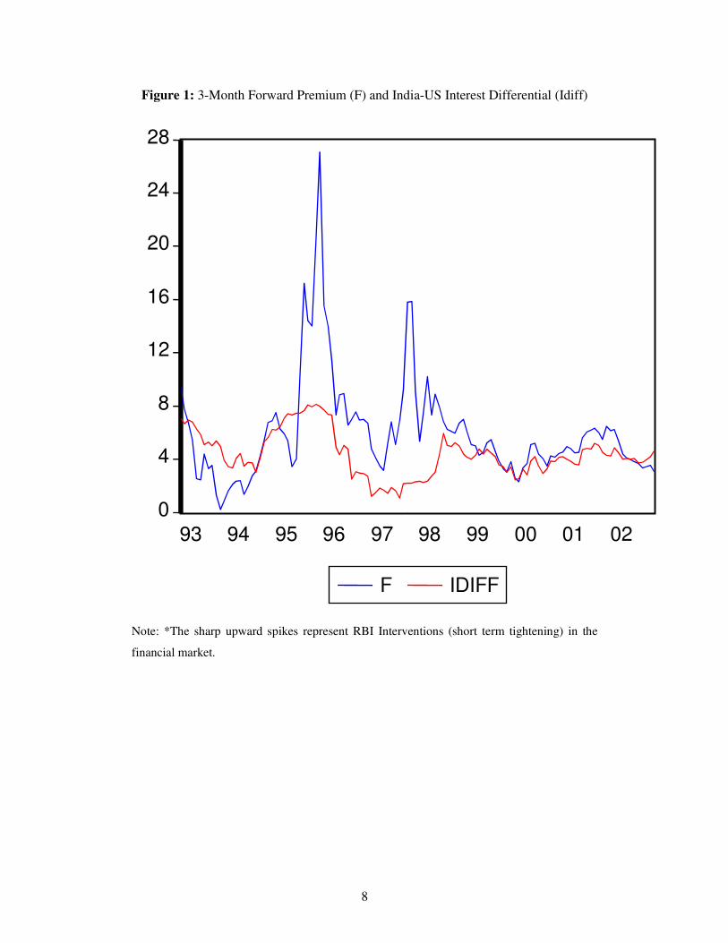
The key variables involved in CIP are plotted in Fig 1.This suggests that the

degree of integration was low till mid-1998 and has increased dramatically since then.

8

Figure 1: 3-Month Forward Premium (F) and India-US Interest Differential (Idiff)

0

4

8

12

16

20

24

28

93 94 95 96 97 98 99 00 01 02

F IDIFF

Note: *The sharp upward spikes represent RBI Interventions (short term tightening) in the

financial market.

9

4 RESULTS

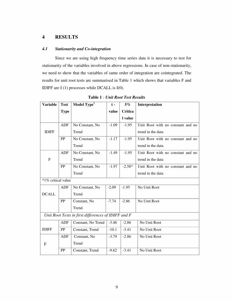
4.1 Stationarity and Co-integration

Since we are using high frequency time series data it is necessary to test for

stationarity of the variables involved in above regressions. In case of non-stationarity,

we need to show that the variables of same order of integration are cointegrated. The

results for unit root tests are summarised in Table 1 which shows that variables F and

IDIFF are I (1) processes while DCALL is I(0).

Table 1 : Unit Root Test Results

Variable Test

Type

Model Type1 t -

value

5%

Critica

l value

Interpretation

ADF No Constant, No

Trend

-1.09 -1.95 Unit Root with no constant and no

trend in the data

IDIFF

PP No Constant, No

Trend

-1.17 -1.95 Unit Root with no constant and no

trend in the data

ADF No Constant, No

Trend

-1.49 -1.95 Unit Root with no constant and no

trend in the data

F

PP No Constant, No

Trend

-1.97 -2.58* Unit Root with no constant and no

trend in the data

*1% critical value

ADF No Constant, No

Trend

-2.09 -1.95 No Unit Root

DCALL

PP Constant, No

Trend

-7.74 -2.86 No Unit Root

Unit Root Tests in first differences of IDIFF and F

ADF Constant, No Trend -3.46 -2.86 No Unit Root

IDIFF PP Constant, Trend -10.1 -3.41 No Unit Root

ADF Constant, No

Trend

-3.79 -2.86 No Unit Root

F

PP Constant, Trend -9.62 -3.41 No Unit Root

10

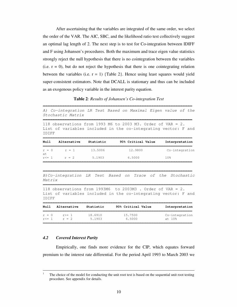
After ascertaining that the variables are integrated of the same order, we select

the order of the VAR. The AIC, SBC, and the likelihood ratio test collectively suggest

an optimal lag length of 2. The next step is to test for Co-integration between IDIFF

and F using Johansen’s procedures. Both the maximum and trace eigen value statistics

strongly reject the null hypothesis that there is no cointegration between the variables

(i.e. r = 0), but do not reject the hypothesis that there is one cointegrating relation

between the variables (i.e. r = 1) {Table 2}. Hence using least squares would yield

super-consistent estimators. Note that DCALL is stationary and thus can be included

as an exogenous policy variable in the interest parity equation.

Table 2: Results of Johansen’s Co-integration Test

--------------------------------------------------------------

A) Co-integration LR Test Based on Maximal Eigen value of the

Stochastic Matrix

--------------------------------------------------------------

118 observations from 1993 M6 to 2003 M3. Order of VAR = 2.

List of variables included in the co-integrating vector: F and

IDIFF

-------------------------------------------------------------- Null Alternative Statistic 90% Critical Value Interpretation

-------------------------------------------------------------- r = 0 r = 1 13.5006 12.9800 Co-integration

at

r<= 1 r = 2 5.1903 6.5000 10%

--------------------------------------------------------------

--------------------------------------------------------------

B)Co-integration LR Test Based on Trace of the Stochastic

Matrix

--------------------------------------------------------------

118 observations from 1993M6 to 2003M3 . Order of VAR = 2.

List of variables included in the co-integrating vector: F and

IDIFF

-------------------------------------------------------------- Null Alternative Statistic 90% Critical Value Interpretation

-------------------------------------------------------------- r = 0 r>= 1 18.6910 15.7500 Co-integration

r<= 1 r = 2 5.1903 6.5000 at 10%

--------------------------------------------------------------

4.2 Covered Interest Parity

Empirically, one finds more evidence for the CIP, which equates forward

premium to the interest rate differential. For the period April 1993 to March 2003 we

1 The choice of the model for conducting the unit root test is based on the sequential unit root testing

procedure. See appendix for details.

11

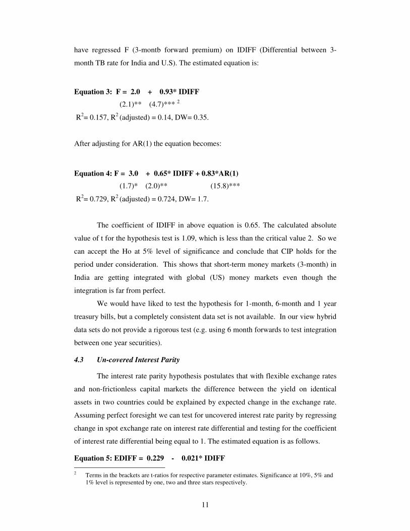
have regressed F (3-montb forward premium) on IDIFF (Differential between 3-

month TB rate for India and U.S). The estimated equation is:

Equation 3: F = 2.0 + 0.93* IDIFF

(2.1)** (4.7)*** 2

R2= 0.157, R2 (adjusted) = 0.14, DW= 0.35.

After adjusting for AR(1) the equation becomes:

Equation 4: F = 3.0 + 0.65* IDIFF + 0.83*AR(1)

(1.7)* (2.0)** (15.8)***

R2= 0.729, R2 (adjusted) = 0.724, DW= 1.7.

The coefficient of IDIFF in above equation is 0.65. The calculated absolute

value of t for the hypothesis test is 1.09, which is less than the critical value 2. So we

can accept the Ho at 5% level of significance and conclude that CIP holds for the

period under consideration. This shows that short-term money markets (3-month) in

India are getting integrated with global (US) money markets even though the

integration is far from perfect.

We would have liked to test the hypothesis for 1-month, 6-month and 1 year

treasury bills, but a completely consistent data set is not available. In our view hybrid

data sets do not provide a rigorous test (e.g. using 6 month forwards to test integration

between one year securities).

4.3 Un-covered Interest Parity

The interest rate parity hypothesis postulates that with flexible exchange rates

and non-frictionless capital markets the difference between the yield on identical

assets in two countries could be explained by expected change in the exchange rate.

Assuming perfect foresight we can test for uncovered interest rate parity by regressing

change in spot exchange rate on interest rate differential and testing for the coefficient

of interest rate differential being equal to 1. The estimated equation is as follows.

Equation 5: EDIFF = 0.229 - 0.021* IDIFF

2 Terms in the brackets are t-ratios for respective parameter estimates. Significance at 10%, 5% and

1% level is represented by one, two and three stars respectively.

12

(1.35) (-0.52)3

R2= 0.006, R2 (adjusted) = -0.021, DW = 1.56.

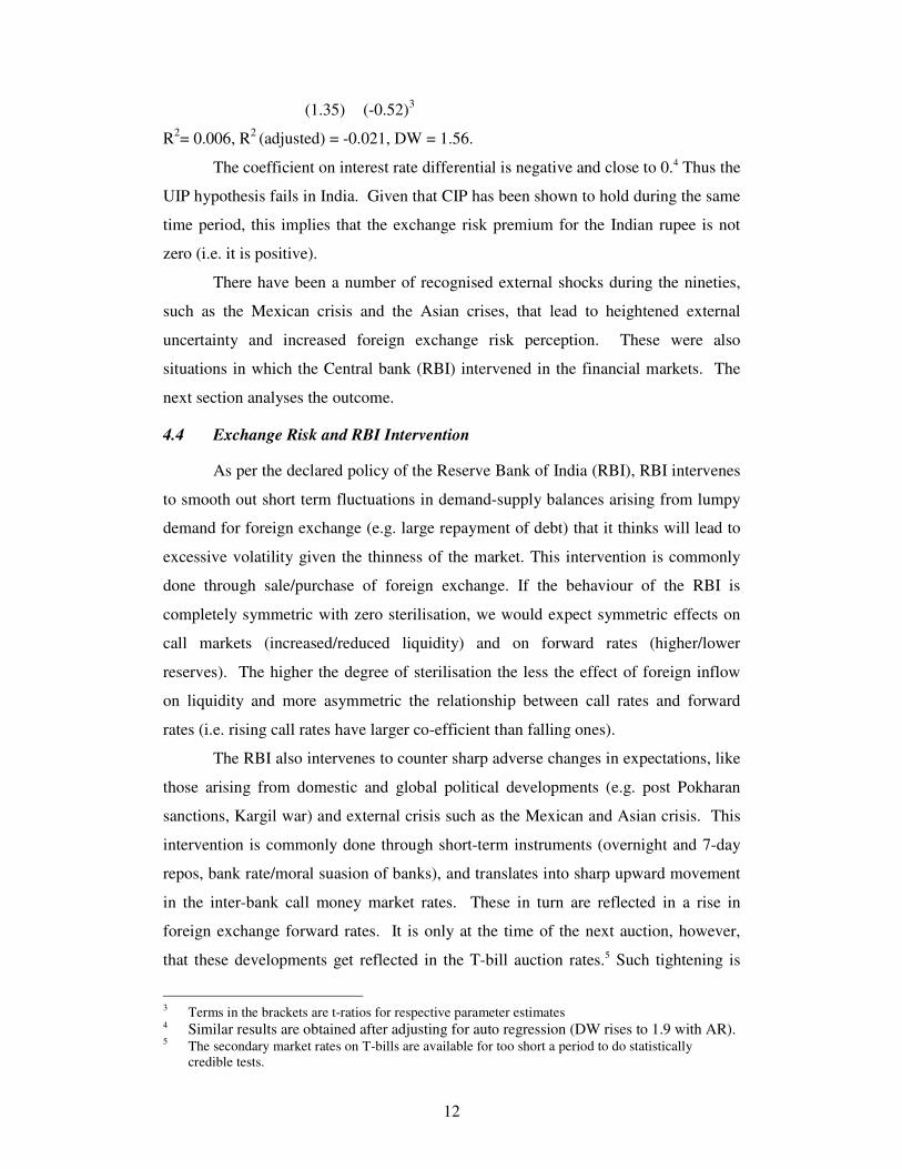
The coefficient on interest rate differential is negative and close to 0.4 Thus the

UIP hypothesis fails in India. Given that CIP has been shown to hold during the same

time period, this implies that the exchange risk premium for the Indian rupee is not

zero (i.e. it is positive).

There have been a number of recognised external shocks during the nineties,

such as the Mexican crisis and the Asian crises, that lead to heightened external

uncertainty and increased foreign exchange risk perception. These were also

situations in which the Central bank (RBI) intervened in the financial markets. The

next section analyses the outcome.

4.4 Exchange Risk and RBI Intervention

As per the declared policy of the Reserve Bank of India (RBI), RBI intervenes

to smooth out short term fluctuations in demand-supply balances arising from lumpy

demand for foreign exchange (e.g. large repayment of debt) that it thinks will lead to

excessive volatility given the thinness of the market. This intervention is commonly

done through sale/purchase of foreign exchange. If the behaviour of the RBI is

completely symmetric with zero sterilisation, we would expect symmetric effects on

call markets (increased/reduced liquidity) and on forward rates (higher/lower

reserves). The higher the degree of sterilisation the less the effect of foreign inflow

on liquidity and more asymmetric the relationship between call rates and forward

rates (i.e. rising call rates have larger co-efficient than falling ones).

The RBI also intervenes to counter sharp adverse changes in expectations, like

those arising from domestic and global political developments (e.g. post Pokharan

sanctions, Kargil war) and external crisis such as the Mexican and Asian crisis. This

intervention is commonly done through short-term instruments (overnight and 7-day

repos, bank rate/moral suasion of banks), and translates into sharp upward movement

in the inter-bank call money market rates. These in turn are reflected in a rise in

foreign exchange forward rates. It is only at the time of the next auction, however,

that these developments get reflected in the T-bill auction rates.5 Such tightening is

3 Terms in the brackets are t-ratios for respective parameter estimates 4 Similar results are obtained after adjusting for auto regression (DW rises to 1.9 with AR). 5 The secondary market rates on T-bills are available for too short a period to do statistically

credible tests.

13

generally followed in due course by a loosening to the starting position, but forwards

may not revert to the original level given the residual uncertainty.

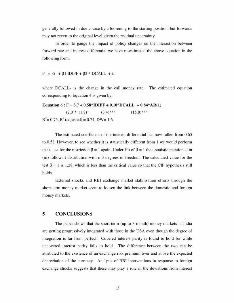
In order to gauge the impact of policy changes on the interaction between

forward rate and interest differential we have re-estimated the above equation in the

following form:

Ft = α + β1 IDIFF + β2 * DCALL + εt

where DCALL- is the change in the call money rate. The estimated equation

corresponding to Equation 4 is given by,

Equation 6 : F = 3.7 + 0.58*IDIFF + 0.10*DCALL + 0.84*AR(1)

(2.0)* (1.8)* (3.4)*** (15.8)***

R2= 0.75, R2 (adjusted) = 0.74, DW= 1.6.

The estimated coefficient of the interest differential has now fallen from 0.65

to 0.58. However, to see whether it is statistically different from 1 we would perform

the t- test for the restriction β = 1 again. Under Ho of β = 1 the t-statistic mentioned in

(iii) follows t-distribution with n-3 degrees of freedom. The calculated value for the

test β = 1 is 1.28, which is less than the critical value so that the CIP hypothesis still

holds.

External shocks and RBI exchange market stabilisation efforts through the

short-term money market seem to loosen the link between the domestic and foreign

money markets.

5 CONCLUSIONS

The paper shows that the short-term (up to 3 month) money markets in India

are getting progressively integrated with those in the USA even though the degree of

integration is far from perfect. Covered interest parity is found to hold for while

uncovered interest parity fails to hold. The difference between the two can be

attributed to the existence of an exchange risk premium over and above the expected

depreciation of the currency. Analysis of RBI interventions in response to foreign

exchange shocks suggests that these may play a role in the deviations from interest

14

parity. Further work needs to be done however on this as well as on instruments of

other maturity such as 1 month and 6 month (for which consistent data was not

available).

15

6 REFERENCES

1. Baillie, R.T. and T. Bollerslev (2000), ‘The forward premium anomaly is not as

bad as you think,’ Journal of International Money and Finance, vol.19 (4) August:

471-88.

2. Bansal, R. and M. Dahquist (2000), ‘The forward premium puzzle: Different tales

from developed and emerging markets,’ Journal of International Economics,

vol.51 (1) : 115-44.

3. Barnhart, S.W., R. McNown, M.S. Wallace (1999), ‘Non-informative tests of the

unbiased forward exchange rate,’ Journal of Financial and Quantitative Analysis,

vol.34 (2) June: 265-91.

4. Christensen, M. (2000), ‘Uncovered interest parity and policy behavior: New

evidence,’ Economics Letters, vol..69 (1) October: 81-87.

5. Cornell, B., 1989, ‘The impact of data errors on measurement of the foreign

exchange risk premium,’ Journal of International Money and Finance, vol.8 ( ) :

147-57.

6. Engel, C. (1996), ‘The forward discount anomaly and the risk premium: A survey

of the recent evidence,’ Journal of Empirical Finance, vol.3 (2): 123-92.

7. Fama, E.F., 1984, ‘Forward and spot exchange rates,’ Journal of Monetary

Economics, vol.14 (3) November: 319-38.

8. Flood, R.P. and A.K. Rose (1996), ‘Fixes: Of the forward discount puzzle,’

Review of Economics and Statistics, vol.78 (4) November: 748-52.

9. Flood, R. P and A K Rose (2002), ‘Uncovered Interest Parity in Crisis,’ IMF Staff

Papers, Vol. 49 (2): 252-66.

10. Frankel, J.A. and K.A. Froot, 1990, ‘Exchange rate forecasting techniques, survey

data, and implications for the foreign exchange market,’ NBER Working paper

no.3470.

11. Froot, K.A. and J.A. Frankel, 1989, ‘Forward discount bias: Is it an exchange risk

premium?’ Quarterly Journal of Economics, vol.104 (1) February: 139-61.

12. Froot, K.A. and R.H. Thaler, 1990, ‘Anomalies: Foreign exchange,’ Journal of

Economic Perspectives, vol.4 (3) : 179-92.

16

13. Gruijters, A.P.D., 1991, ‘De efficientie van valutamarkten: een overzicht,’

Maandschrift Economie, vol.55 (4): 244-67.

14. Hodrick, R., 1987, The Empirical Evidence on the Efficiency of Forward and

Futures Foreign Exchange Markets, Harwood 1987.

15. Lewis, K.K., 1995, ‘Puzzles in international financial markets,’ in G. Grossman,

K. Rogoff (eds.) Handbook of International Economics, vol.3. Elsevier: 1913-71.

16. Mayfield, E.S. and R.G. Murphy (1992), ‘Interest rate parity and the exchange

risk premium: Evidence from panel data,’ Economics Letters, vol.40 (3)

November: 319-24

17. McCallum, B.T., 1994, ‘A reconsideration of the uncovered interest parity

relationship,’ Journal of Monetary Economics, vol.33 (1) February: 105-32.

18. McFarland, J.W., P.C. McMahon and Y. Ngama (1994), ‘Forward exchange rates

and expectations during the 1920s: A re-examination of the evidence,’ Journal of

International Finance, vol.13 (6) December: 627-36.

19. Phillips, P.C.B., J.W. McFarland and P.C. McMahon, 1996, ‘Robust tests of

forward exchange market efficiency with empirical evidence from the 1920’s,’

Journal of Applied Econometrics, vol.11 (1) Jan-Feb: 1-22.

20. Varma, J.R. (1997), Indian money market: market structure, covered parity

and term structure. The ICFAI Journal of Applied Finance, 3(2),1-10.

17

7 APPENDIX: TESTS

7.1 Order of integration

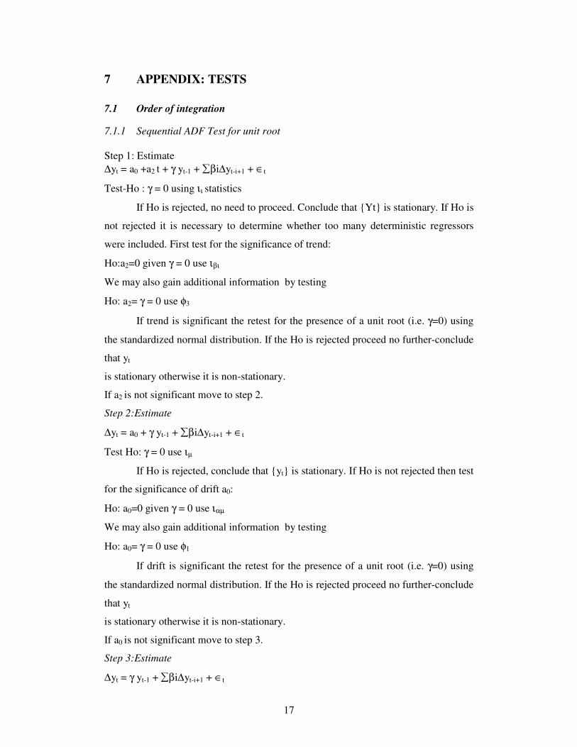
7.1.1 Sequential ADF Test for unit root

Step 1: Estimate

∆yt = a0 +a2 t + γ yt-1 + ∑βi∆yt-i+1 + ∈t

Test-Ho : γ = 0 using ιι statistics

If Ho is rejected, no need to proceed. Conclude that {Yt} is stationary. If Ho is

not rejected it is necessary to determine whether too many deterministic regressors

were included. First test for the significance of trend:

Ho:a2=0 given γ = 0 use ιβι

We may also gain additional information by testing

Ho: a2= γ = 0 use φ3

If trend is significant the retest for the presence of a unit root (i.e. γ=0) using

the standardized normal distribution. If the Ho is rejected proceed no further-conclude

that yt

is stationary otherwise it is non-stationary.

If a2 is not significant move to step 2.

Step 2:Estimate

∆yt = a0 + γ yt-1 + ∑βi∆yt-i+1 + ∈t

Test Ho: γ = 0 use ιµ

If Ho is rejected, conclude that {yt} is stationary. If Ho is not rejected then test

for the significance of drift a0:

Ho: a0=0 given γ = 0 use ιαµ

We may also gain additional information by testing

Ho: a0= γ = 0 use φ1

If drift is significant the retest for the presence of a unit root (i.e. γ=0) using

the standardized normal distribution. If the Ho is rejected proceed no further-conclude

that yt

is stationary otherwise it is non-stationary.

If a0 is not significant move to step 3.

Step 3:Estimate

∆yt = γ yt-1 + ∑βi∆yt-i+1 + ∈t

18

Test Ho: γ = 0 use ι

If Ho is rejected, conclude that {yt} is stationary otherwise it is nonstationary.

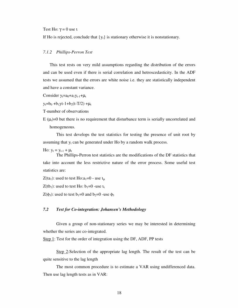
7.1.2 Phillips-Perron Test

This test rests on very mild assumptions regarding the distribution of the errors

and can be used even if there is serial correlation and hetroscedasticity. In the ADF

tests we assumed that the errors are white noise i.e. they are statistically independent

and have a constant variance.

Consider yt=a0+a1yt-1+µt

yt=b0 +b1yt-1+b2(t-T/2) +µt

T-number of observations

E (µt)=0 but there is no requirement that disturbance term is serially uncorrelated and

homogeneous.

This test develops the test statistics for testing the presence of unit root by

assuming that yt can be generated under Ho by a random walk process.

Ho: yt = yt-1 + µt

The Phillips-Perron test statistics are the modifications of the DF statistics that

take into account the less restrictive nature of the error process. Some useful test

statistics are:

Z(ta1): used to test Ho:a1=0 - use ιµ

Z(tb1): used to test Ho: b1=0 -use ιι

Z(φ3): used to test b1=0 and b2=0 -use φ3

7.2 Test for Co-integration: Johansen’s Methodology

Given a group of non-stationary series we may be interested in determining

whether the series are co-integrated.

Step 1: Test for the order of integration using the DF, ADF, PP tests

Step 2:Selection of the appropriate lag length. The result of the test can be

quite sensitive to the lag length

The most common procedure is to estimate a VAR using undifferenced data.

Then use lag length tests as in VAR:

19

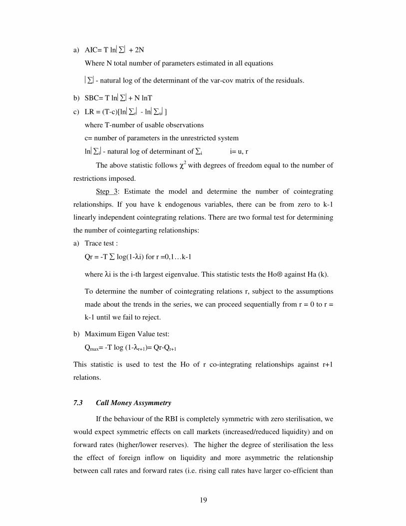
a) AIC= T ln∑ + 2N

Where N total number of parameters estimated in all equations

∑- natural log of the determinant of the var-cov matrix of the residuals.

b) SBC= T ln∑+ N lnT

c) LR = (T-c)[ln∑r - ln∑u]

where T-number of usable observations

c= number of parameters in the unrestricted system

ln∑i- natural log of determinant of ∑i i= u, r

The above statistic follows χ2 with degrees of freedom equal to the number of

restrictions imposed.

Step 3: Estimate the model and determine the number of cointegrating

relationships. If you have k endogenous variables, there can be from zero to k-1

linearly independent cointegrating relations. There are two formal test for determining

the number of cointegarting relationships:

a) Trace test :

Qr = -T ∑ log(1-λi) for r =0,1…k-1

where λi is the i-th largest eigenvalue. This statistic tests the Ho® against Ha (k).

To determine the number of cointegrating relations r, subject to the assumptions

made about the trends in the series, we can proceed sequentially from r = 0 to r =

k-1 until we fail to reject.

b) Maximum Eigen Value test:

Qmax= -T log (1-λr+1)= Qr-Qr+1

This statistic is used to test the Ho of r co-integrating relationships against r+1

relations.

7.3 Call Money Assymmetry

If the behaviour of the RBI is completely symmetric with zero sterilisation, we

would expect symmetric effects on call markets (increased/reduced liquidity) and on

forward rates (higher/lower reserves). The higher the degree of sterilisation the less

the effect of foreign inflow on liquidity and more asymmetric the relationship

between call rates and forward rates (i.e. rising call rates have larger co-efficient than

20

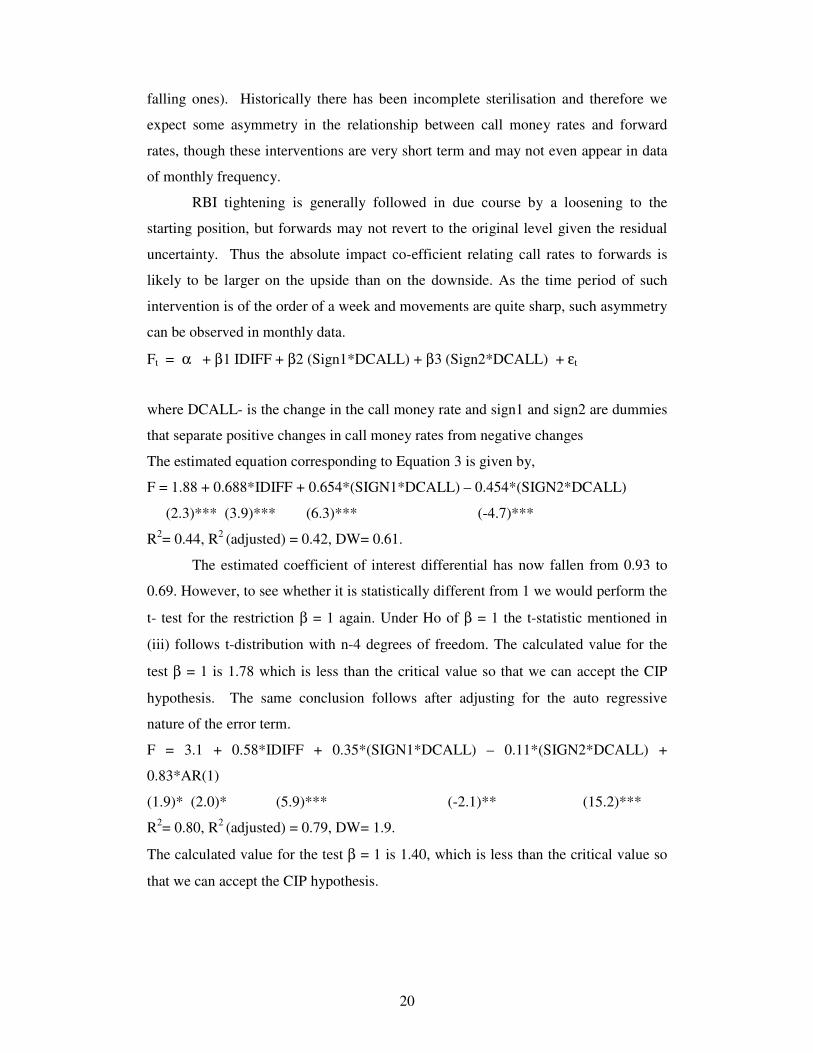
falling ones). Historically there has been incomplete sterilisation and therefore we

expect some asymmetry in the relationship between call money rates and forward

rates, though these interventions are very short term and may not even appear in data

of monthly frequency.

RBI tightening is generally followed in due course by a loosening to the

starting position, but forwards may not revert to the original level given the residual

uncertainty. Thus the absolute impact co-efficient relating call rates to forwards is

likely to be larger on the upside than on the downside. As the time period of such

intervention is of the order of a week and movements are quite sharp, such asymmetry

can be observed in monthly data.

Ft = α + β1 IDIFF + β2 (Sign1*DCALL) + β3 (Sign2*DCALL) + εt

where DCALL- is the change in the call money rate and sign1 and sign2 are dummies

that separate positive changes in call money rates from negative changes

The estimated equation corresponding to Equation 3 is given by,

F = 1.88 + 0.688*IDIFF + 0.654*(SIGN1*DCALL) – 0.454*(SIGN2*DCALL)

(2.3)*** (3.9)*** (6.3)*** (-4.7)***

R2= 0.44, R2 (adjusted) = 0.42, DW= 0.61.

The estimated coefficient of interest differential has now fallen from 0.93 to

0.69. However, to see whether it is statistically different from 1 we would perform the

t- test for the restriction β = 1 again. Under Ho of β = 1 the t-statistic mentioned in

(iii) follows t-distribution with n-4 degrees of freedom. The calculated value for the

test β = 1 is 1.78 which is less than the critical value so that we can accept the CIP

hypothesis. The same conclusion follows after adjusting for the auto regressive

nature of the error term.

F = 3.1 + 0.58*IDIFF + 0.35*(SIGN1*DCALL) – 0.11*(SIGN2*DCALL) +

0.83*AR(1)

(1.9)* (2.0)* (5.9)*** (-2.1)** (15.2)***

R2= 0.80, R2 (adjusted) = 0.79, DW= 1.9.

The calculated value for the test β = 1 is 1.40, which is less than the critical value so

that we can accept the CIP hypothesis.