global impact study june 2008 pg economics
TRANSCRIPT

GM crops: global socio-economic and environmental impacts 1996-2006
Graham Brookes & Peter Barfoot
PG Economics Ltd, UK
Dorchester, UK June 2008

GM crop impact: 1996-2006
©PG Economics Ltd 2008 2
Table of contents Executive summary and conclusions.........................................................................................................7 1 Introduction..............................................................................................................................................17
1.1 Objectives ..........................................................................................................................................17 1.2 Methodology.....................................................................................................................................17 1.3 Structure of report ............................................................................................................................18
2 Global context of GM crops....................................................................................................................19 2.1 Global plantings ...............................................................................................................................19 2.2 Plantings by crop and trait..............................................................................................................19
2.2.1 By crop........................................................................................................................................19 2.2.2 By trait ........................................................................................................................................20 2.2.3 By country..................................................................................................................................21
3 The farm level economic impact of GM crops 1996-2006...................................................................24 3.1 Herbicide tolerant soybeans ...........................................................................................................24
3.1.1 The US ........................................................................................................................................24 3.1.2 Argentina ...................................................................................................................................26 3.1.3 Brazil ...........................................................................................................................................27 3.1.4 Paraguay and Uruguay............................................................................................................28 3.1.5 Canada........................................................................................................................................29 3.1.6 South Africa ...............................................................................................................................30 3.1.7 Romania .....................................................................................................................................30 3.1.8 Mexico ........................................................................................................................................31 3.1.9 Summary of global economic impact.....................................................................................32
3.2 Herbicide tolerant maize .................................................................................................................33 3.2.1 The US ........................................................................................................................................33 3.2.2 Canada........................................................................................................................................34 3.2.3 Argentina ...................................................................................................................................35 3.2.4 South Africa ...............................................................................................................................35 3.2.5 Philippines .................................................................................................................................35 3.2.6 Summary of global economic impact.....................................................................................35
3.3 Herbicide tolerant cotton.................................................................................................................36 3.3.1 The US ........................................................................................................................................36 3.3.2 Other countries..........................................................................................................................37 3.3.3 Summary of global economic impact.....................................................................................37
3.4 Herbicide tolerant canola ................................................................................................................37 3.4.1 Canada........................................................................................................................................37 3.4.2 The US ........................................................................................................................................39 3.4.3 Summary of global economic impact.....................................................................................40
3.5 GM Insect resistant (GM IR) maize................................................................................................40 3.5.1 US ................................................................................................................................................40 3.5.2 Canada........................................................................................................................................41 3.5.3 Argentina ...................................................................................................................................41 3.5.4 South Africa ...............................................................................................................................42 3.5.5 Spain ...........................................................................................................................................42 3.5.6 Other countries..........................................................................................................................43 3.5.7 Summary of economic impact.................................................................................................44

GM crop impact: 1996-2006
©PG Economics Ltd 2008 3
3.6 Insect resistant (Bt) cotton (GM IR)................................................................................................44 3.6.1 The US ........................................................................................................................................44 3.6.2 China...........................................................................................................................................45 3.6.3 Australia.....................................................................................................................................46 3.6.4 Argentina ...................................................................................................................................47 3.6.5 Mexico ........................................................................................................................................47 3.6.6 South Africa ...............................................................................................................................48 3.6.7 India ............................................................................................................................................49 3.6.8 Brazil ...........................................................................................................................................50 3.6.9 Other countries..........................................................................................................................50 3.6.9 Summary of global impact.......................................................................................................50
3.7 Other GM crops ................................................................................................................................51 3.7.1 Maize/corn rootworm resistance ............................................................................................51 3.7.2 Virus resistant papaya..............................................................................................................51 3.7.3 Virus resistant squash ..............................................................................................................51 3.7.4 Insect resistant potatoes ...........................................................................................................52
3.8 Other farm level economic impacts of using GM crops..............................................................52 3.9 GM technology adoption and size of farm ...................................................................................53 3.10 Trade flows and related issues .....................................................................................................54
4 The environmental impact of GM crops...............................................................................................58 4.1 Use of insecticides and herbicides .................................................................................................58
4.1.1 GM herbicide tolerant (to glyphosate) soybeans (GM HT).................................................58 4.1.2 Herbicide tolerant maize..........................................................................................................66 4.1.3 Herbicide tolerant cotton .........................................................................................................70 4.1.4 Herbicide tolerant canola.........................................................................................................74 4.1.6 GM insect resistant (Bt) maize.................................................................................................76 4.1.7 GM insect resistant (Bt) cotton ................................................................................................79 4.1.8 Other environmental impacts - possible development of herbicide resistant weeds and weed shifts ..........................................................................................................................................85
4.2 Carbon sequestration.......................................................................................................................87 4.2.1 Tractor fuel use..........................................................................................................................88 4.2.2 Soil carbon sequestration .........................................................................................................89 4.2.3 Herbicide tolerance and conservation tillage........................................................................92 4.2.4 Herbicide tolerant soybeans ....................................................................................................93 4.2.5 Herbicide tolerant canola.........................................................................................................99 4.2.6 Herbicide tolerant cotton and maize....................................................................................100 4.2.7 Insect resistant cotton .............................................................................................................101 4.2.8 Insect resistant maize..............................................................................................................101 4.2.9 Summary of carbon sequestration impact...........................................................................102
Appendix 1: Argentine second crop soybeans .....................................................................................104 Appendix 2: The Environmental Impact Quotient (EIQ): a method to measure the environmental impact of pesticides..................................................................................................................................105 Appendix 3: Additional information relating to the environmental impact....................................109 References..................................................................................................................................................115
GM crop impact: 1996-2006
©PG Economics Ltd 2008 4
Table of tables Table 1: Global farm income benefits from growing GM crops 1996-2006: million US $...................8 Table 2: GM crop farm income benefits 1996-2006 selected countries: million US $...........................8 Table 3: GM crop farm income benefits 2006: developing versus developed countries: million US
$ ..............................................................................................................................................................9 Table 4: Cost of accessing GM technology (million $) relative to the total farm income benefits
2006 ......................................................................................................................................................10 Table 5: Impact of changes in the use of herbicides and insecticides from growing GM crops
globally 1996-2006..............................................................................................................................13 Table 6: Reduction in environmental impact from changes in pesticide use associated with GM
crop adoption by country 1996-2006 selected countries: % reduction in field EIQ values......13 Table 7: GM crop environmental benefits from lower insecticide and herbicide use 2006:
developing versus developed countries .........................................................................................14 Table 8: Context of carbon sequestration impact 2006: car equivalents..............................................15 Table 9: Global GM plantings by country 1996-2006 (‘000 hectares) ...................................................22 Table 10: GM technology share of crop plantings in 2006 by country (% of total plantings) ..........22 Table 11: Farm level income impact of using GM HT soybeans in the US 1996-2006.......................25 Table 12: Farm level income impact of using GM HT soybeans in Argentina 1996-2006 ................27 Table 13: Farm level income impact of using GM HT soybeans in Brazil 1997-2006 ........................28 Table 14: Farm level income impact of using GM HT soybeans in Canada 1997-2006.....................29 Table 15: Farm level income impact of using GM HT soybeans in South Africa 2001-2006 ............30 Table 16: Farm level income impact of using herbicide tolerant soybeans in Romania 1999-2006 .31 Table 17: Farm level income impact of using GM HT soybeans in Mexico 2004-2006......................32 Table 18: Farm level income impact of using GM HT canola in Canada 1996-2006..........................38 Table 19: Farm level income impact of using GM IR maize in the US 1996-2006..............................40 Table 20: Farm level income impact of using GM IR maize in South Africa 2000-2006....................42 Table 21: Farm level income impact of using GM IR maize in Spain 1998-2006................................43 Table 22: Farm level income impact of using GM IR cotton in the US 1996-2006..............................44 Table 23: Farm level income impact of using GM IR cotton in China 1997-2006...............................45 Table 24: Farm level income impact of using GM IR cotton in Australia 1996-2006.........................46 Table 25: Farm level income impact of using GM IR cotton in Mexico 1996-2006 ............................48 Table 26: Farm level income impact of using GM IR cotton in India 2002-2006................................50 Table 27: Additional production of main crops in 2006 due to GM technology (million tonnes)...54 Table 28: Share of global crop trade accounted for GM production 2006/7 (million tonnes)...........55 Table 29: Share of global crop derivative (meal) trade accounted for GM production 2006/7
(million tonnes) ..................................................................................................................................56 Table 30: Herbicide usage on soybeans in the US 1996-2006................................................................59 Table 31: Herbicide usage on GM HT and conventional soybeans in the US 1996-2006..................59 Table 32: National level changes in herbicide ai use and field EIQ values for GM HT soybeans in
the US 1996-2006 ................................................................................................................................61 Table 33: National level changes in herbicide ai use and field EIQ values for GM HT soybeans in
Canada 1996-2006 ..............................................................................................................................61 Table 34: National level changes in herbicide ai use and field EIQ values for GM HT soybeans in
Brazil 1997-2006..................................................................................................................................62 Table 35: National level changes in herbicide ai use and field EIQ values for GM HT soybeans in
Romania 1999-2006 ............................................................................................................................64 Table 36: Herbicide usage on maize in the US 1996-2006 .....................................................................66
GM crop impact: 1996-2006
©PG Economics Ltd 2008 5
Table 37: Average US maize herbicide usage and environmental load 1997-2006: conventional and GM HT.........................................................................................................................................66
Table 38: National level changes in herbicide ai use and field EIQ values for GM HT maize in the US 1997-2006.......................................................................................................................................67
Table 39: Change in herbicide use and environmental load from using GM HT maize in Canada 1999-2006.............................................................................................................................................68
Table 40: Herbicide usage on cotton in the US 1996-2006 .....................................................................70 Table 41: Herbicide usage and its associated environmental load: GM HT and conventional cotton
in the US 1997-2006............................................................................................................................70 Table 42: National level changes in herbicide ai use and field EIQ values for GM HT cotton in the
US 1997-2006.......................................................................................................................................71 Table 43: National level changes in herbicide ai use and field EIQ values for GM HT cotton in
Australia 2000-2006 (negative sign denotes increase in use) .......................................................72 Table 44: Average US maize insecticide usage and its environmental load 1996-2006: conventional
versus GM...........................................................................................................................................76 Table 45: National level changes in insecticide ai use and field EIQ values for GM IR maize in the
US 1996-2006.......................................................................................................................................76 Table 46: Average US cotton insecticide usage and environmental impact 1996-2006: conventional
versus GM...........................................................................................................................................80 Table 47: National level changes in insecticide ai use and field EIQ values for GM IR cotton in the
US 1996-2006.......................................................................................................................................80 Table 48: National level changes in insecticide ai use and field EIQ values for GM IR cotton in
China 1997-2006 .................................................................................................................................81 Table 49: Comparison of insecticide ai use and field EIQ values for conventional, Ingard and
Bollgard II cotton in Australia..........................................................................................................82 Table 50: National level changes in insecticide ai use and field EIQ values for GM IR cotton in
Australia 1996-2006............................................................................................................................82 Table 51: National level changes in insecticide ai use and field EIQ values for GM IR cotton in
Argentina 1998-2006 ..........................................................................................................................83 Table 52 Total farm diesel fuel consumption estimate (in litres per year/ha) ....................................88 Table 53: Tractor fuel consumption by tillage method..........................................................................89 Table 54: Summary of the potential; of NT cultivation systems ..........................................................91 Table 55: US soybean tillage practices and the adoption of GM HT cultivars 1996-2006 (million ha)
..............................................................................................................................................................93 Table 56: US soybean consumption of tractor fuel used for tillage 1996-2006 ...................................94 Table 57: US soybeans: permanent reduction in tractor fuel consumption and reduction in CO2
emissions.............................................................................................................................................94 Table 58: US soybeans: potential soil carbon sequestration (1996 to 2006).........................................95 Table 59: US soybeans: potential additional soil carbon sequestration (1996 to 2006)......................95 Table 60: Argentina soybean tillage practices and the adoption of GM cultivars 1996-2006 (million
ha) ........................................................................................................................................................96 Table 61: Argentine soybeans: permanent reduction in tractor fuel consumption and reduction in
CO2 emissions ....................................................................................................................................97 Table 62: Argentine soybeans: potential additional soil carbon sequestration (1996 to 2006) .........98 Table 63: Canadian canola: permanent reduction in tractor fuel consumption and reduction in
CO2 emissions ....................................................................................................................................99 Table 64: Canada canola: potential additional soil carbon sequestration (1996 to 2006) ................100
GM crop impact: 1996-2006
©PG Economics Ltd 2008 6
Table 65: Permanent reduction in global tractor fuel consumption and CO2 emissions resulting from the cultivation of GM insect resistant cotton......................................................................101
Table 66: Summary of carbon sequestration impact 1996-2006..........................................................102 Table 67: Context of carbon sequestration impact 2006: car equivalents..........................................103
Table of figures Figure 1: GM crop plantings 2006 by crop (base area: 99.6 million hectares) ....................................19 Figure 2: 2006’s share of GM crops in global plantings of key crops (hectares) ................................20 Figure 3: Global GM crop plantings by crop 1996-2006 (hectares) ......................................................20 Figure 4: Global GM crop plantings by main trait and crop: 2006.......................................................21 Figure 5: Global GM crop plantings 2006 by country............................................................................21 Figure 6: National farm income benefit from using GM HT soybeans in Paraguay and Uruguay
1999-2006 (million $)..........................................................................................................................29 Figure 7: Global farm level income benefits derived from using GM HT soybeans 1996-2006
(million $)............................................................................................................................................33 Figure 8: National farm income impact of using GM HT maize in the US 1997-2006 ......................34 Figure 9: National farm income impact of using GM HT maize in Canada 1999-2006 ($ million) .34 Figure 10: National farm income impact of using GM HT cotton in the US 1997-2006....................36 Figure 11: National farm income impact of using GM HT canola in the US 1999-2006....................39 Figure 12: National farm income impact of using GM IR maize in Canada 1996-2006 ....................41 Figure 13: National farm income impact of using GM IR cotton in Argentina 1998-2006 ...............47 Figure 14: National farm income impact of using GM IR cotton in South Africa 1998-2006 ...........49 Figure 15: Reduction in herbicide use and the environmental load from using GM HT soybeans in
all adopting countries 1996-2006 .....................................................................................................65 Figure 16: Reduction in herbicide use and the environmental load from using GM HT maize in
adopting countries 1997-2006...........................................................................................................69 Figure 17: Reduction in herbicide use and the environmental load from using GM HT cotton in
the US, Australia, Argentina and South Africa 1997-2006 ...........................................................74 Figure 18: Reduction in herbicide use and the environmental load from using GM HT canola in
the US and Canada 1996-2006 ..........................................................................................................75 Figure 19: Reduction in insecticide use and the environmental load from using GM IR maize in
adopting countries 1996-2006...........................................................................................................79 Figure 20: Reduction in insecticide use and the environmental load from using GM IR cotton in
adopting countries 1996-2006...........................................................................................................85
GM crop impact: 1996-2006
©PG Economics Ltd 2008 7
Executive summary and conclusions This study presents the findings of research into the global socio-economic and environmental impact of GM crops in the eleven years since they were first commercially planted on a significant area. It focuses on the farm level economic effects, the environmental impact resulting from changes in the use of insecticides and herbicides, and the contribution towards reducing greenhouse gas (GHG) emissions. Background context The analysis presented is largely based on the average performance and impact recorded in different crops. The economic performance and environmental impact of the technology at the farm level does, however vary widely, both between and within regions/countries. This means that the impact of this technology (and any new technology, GM or otherwise) is subject to variation at the local level. Also the performance and impact should be considered on a case by case basis in terms of crop and trait combinations. Agricultural production systems (how farmers use different and new technologies and husbandry practices) are dynamic and vary with time. This analysis seeks to address this issue, wherever possible, by comparing GM production systems with the most likely conventional alternative, if GM technology had not been available. This is of particular relevance to the case of GM herbicide tolerant (GM HT) soybeans, where prior to the introduction of GM HT technology, production systems were already switching away from conventional to no/low tillage production (in which the latter systems make greater use of, and are more reliant on, herbicide-based weed control systems - the role of GM HT technology in facilitating this fundamental change in production systems is assessed below). In addition, the market dynamic impact of GM crop adoption (on prices) has been incorporated into the analysis by use of current prices (for each year) for all crops. Farm income effects1 The impact on farm incomes in the GM adopting countries has been very positive (Table 1). This derives from enhanced productivity and efficiency gains:
• In 2006, the direct farm income benefit was $6.21 billion. If the additional income arising from second crop soybeans in Argentina & Paraguay is also taken into consideration2, this income gain rises to $6.94 billion. This is equivalent to having added between 3.4% and 3.8% to the value of global production of the four main crops of soybeans, maize, canola and cotton;
• Since 1996, farm incomes have benefited by $30.3 billion ($33.8 billion inclusive of second crop soybean gains in Argentina);
• The largest gains in farm income have arisen in the soybean sector, where the additional income generated by GM HT soybeans in 2006 has been equivalent to adding 6.7% to value of the crop in the GM growing countries, or adding the equivalent of 5.6% to the value of the global soybean crop;
1 See section 3 for details 2 The availability of GM HT technology has played a major role in facilitating the expansion of second crop soybeans, usually following on from wheat (in the same season)
GM crop impact: 1996-2006
©PG Economics Ltd 2008 8
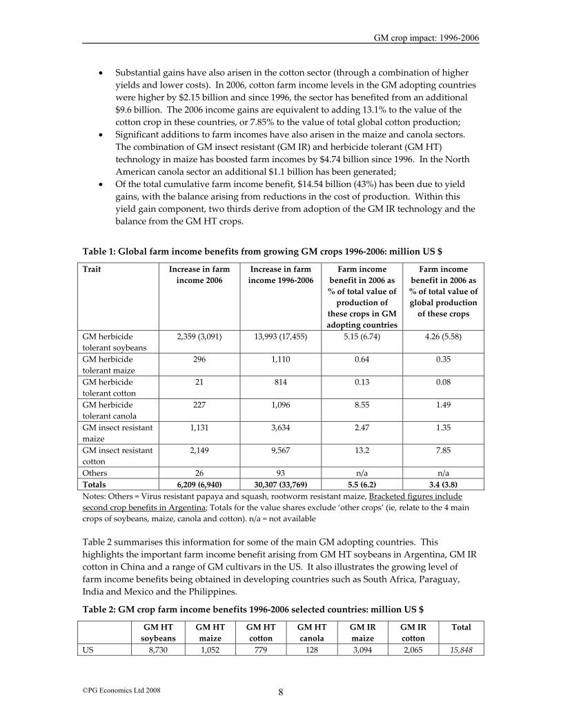
• Substantial gains have also arisen in the cotton sector (through a combination of higher yields and lower costs). In 2006, cotton farm income levels in the GM adopting countries were higher by $2.15 billion and since 1996, the sector has benefited from an additional $9.6 billion. The 2006 income gains are equivalent to adding 13.1% to the value of the cotton crop in these countries, or 7.85% to the value of total global cotton production;
• Significant additions to farm incomes have also arisen in the maize and canola sectors. The combination of GM insect resistant (GM IR) and herbicide tolerant (GM HT) technology in maize has boosted farm incomes by $4.74 billion since 1996. In the North American canola sector an additional $1.1 billion has been generated;
• Of the total cumulative farm income benefit, $14.54 billion (43%) has been due to yield gains, with the balance arising from reductions in the cost of production. Within this yield gain component, two thirds derive from adoption of the GM IR technology and the balance from the GM HT crops.
Table 1: Global farm income benefits from growing GM crops 1996-2006: million US $
Trait Increase in farm income 2006
Increase in farm income 1996-2006
Farm income benefit in 2006 as % of total value of
production of these crops in GM adopting countries
Farm income benefit in 2006 as % of total value of global production
of these crops
GM herbicide tolerant soybeans
2,359 (3,091) 13,993 (17,455) 5.15 (6.74) 4.26 (5.58)
GM herbicide tolerant maize
296 1,110 0.64 0.35
GM herbicide tolerant cotton
21 814 0.13 0.08
GM herbicide tolerant canola
227 1,096 8.55 1.49
GM insect resistant maize
1,131 3,634 2.47 1.35
GM insect resistant cotton
2,149 9,567 13.2 7.85
Others 26 93 n/a n/a Totals 6,209 (6,940) 30,307 (33,769) 5.5 (6.2) 3.4 (3.8) Notes: Others = Virus resistant papaya and squash, rootworm resistant maize, Bracketed figures include second crop benefits in Argentina; Totals for the value shares exclude ‘other crops’ (ie, relate to the 4 main crops of soybeans, maize, canola and cotton). n/a = not available Table 2 summarises this information for some of the main GM adopting countries. This highlights the important farm income benefit arising from GM HT soybeans in Argentina, GM IR cotton in China and a range of GM cultivars in the US. It also illustrates the growing level of farm income benefits being obtained in developing countries such as South Africa, Paraguay, India and Mexico and the Philippines.
Table 2: GM crop farm income benefits 1996-2006 selected countries: million US $
GM HT soybeans
GM HT maize
GM HT cotton
GM HT canola
GM IR maize
GM IR cotton
Total
US 8,730 1,052 779 128 3,094 2,065 15,848

GM crop impact: 1996-2006
©PG Economics Ltd 2008 9
Argentina 6,250 22 25 N/a 193 107 6,597 Brazil 1,912 N/a N/a N/a N/a 17 1,929 Paraguay 349 N/a N/a N/a N/a N/a 349 Canada 87 32 N/a 968 145 N/a 1,232 South Africa
3 2.5 0.2 N/a 132 18 155.7
China N/a N/a N/a N/a N/a 5,823 5,823 India N/a N/a N/a N/a N/a 1,294 1,294 Australia N/a N/a 4.8 N/a N/a 179 183.8 Mexico 5.1 N/a 6 N/a N/a 59.5 70.6 Philippines N/a 1.5 N/a N/a 27.3 N/a 28.8 Spain N/a N/a N/a N/a 39.4 N/a 39.4 Note: Argentine GM HT soybeans include second crop soybeans benefits. N/a = not applicable In terms of the division of the economic benefits obtained by farmers in developing countries relative to farmers in developed countries, Table 3 shows that in 2006, the majority of the farm income benefits (54%) have been earned by developing country farmers. The vast majority of these income gains for developing country farmers have been from GM IR cotton and GM HT soybeans.
Table 3: GM crop farm income benefits 2006: developing versus developed countries: million US $
Developed Developing % developed % developing GM HT soybeans 1,263 1,828 40.9 59.1 GM IR maize 992 139 87.8 12.2 GM HT maize 274 22 92.7 7.3 GM IR cotton 434 1,715 20.2 79.8 GM HT cotton 12 9 57.4 42.6 GM HT canola 227 0 100 0 GM VR papaya and squash
26 0 100 0
Total 3,228 3,713 46.5 53.5 Developing countries include all countries in South America Cumulatively over the period 1996 to 2006, developing country farmers have acquired 49% of the total ($34 billion) farm income benefit. Examination of the cost farmers pay for accessing GM technology relative to the total gains derived, Table 4 shows that across the four main GM crops, the total cost in 2006 was equal to 28% of the total technology gains (inclusive of farm income gains plus cost of the technology payable to the seed supply chain3). For farmers in developing countries the total cost was equal to about 17% of total technology gains, whilst for farmers in developed countries the cost was 38% of the total technology gains. Whilst circumstances vary between countries, the higher share of total technology gains accounted for by farm income gains in developing countries relative to the farm income share in
3 The cost of the technology accrues to the seed supply chain including sellers of seed to farmers, seed multipliers, plant breeders, distributors and the GM technology providers

GM crop impact: 1996-2006
©PG Economics Ltd 2008 10
developed countries reflects factors such as weaker provision and enforcement of intellectual property rights in developing countries.
Table 4: Cost of accessing GM technology (million $) relative to the total farm income benefits 2006
Cost of technology: all farmers
Farm income
gain: all
farmers
Total benefit of technology to farmers and
seed supply chain
Cost of technology: developing countries
Farm income gain: developing countries
Total benefit of technology to
farmers and seed supply chain: developing countries
GM HT soybeans
1,000 3,091 4,091 284 1,828 2,112
GM IR maize
436 1,131 1,567 61 139 200
GM HT maize
223 296 519 10 22 32
GM IR cotton
576 2,149 2,725 375 1,715 2,090
GM HT cotton
290 21 311 12 9 21
GM HT canola
162 227 389 0 0 0
Total 2,687 6,915 9,602 742 3,713 4,455 N/a = not applicable. Cost of accessing the technology is based on the seed premia paid by farmers for
using GM technology relative to its conventional equivalents. Total farm income gain excludes £26 million associated with virus resistant crops in the US
As well as these quantifiable impacts on farm profitability, there have been other important, more intangible impacts (of an economic nature). Most of these have been important influences for adoption of the technology. These include: Herbicide tolerant crops
• Increased management flexibility that comes from a combination of the ease of use associated with broad-spectrum, post-emergent herbicides like glyphosate and the increased/longer time window for spraying;
• Compared to conventional crops, where post-emergent herbicide application may result in ‘knock-back’ (some risk of crop damage from the herbicide), this problem is less likely to occur in GM HT crops;
• Facilitation of adoption of no/reduced tillage practices with resultant savings in time and equipment usage (see below for environmental benefits);
• Improved weed control has reduced harvesting costs – cleaner crops have resulted in reduced times for harvesting. It has also improved harvest quality and led to higher levels of quality price bonuses in some regions;
• Elimination of potential damage caused by soil-incorporated residual herbicides in follow-on crops.
GM crop impact: 1996-2006
©PG Economics Ltd 2008 11
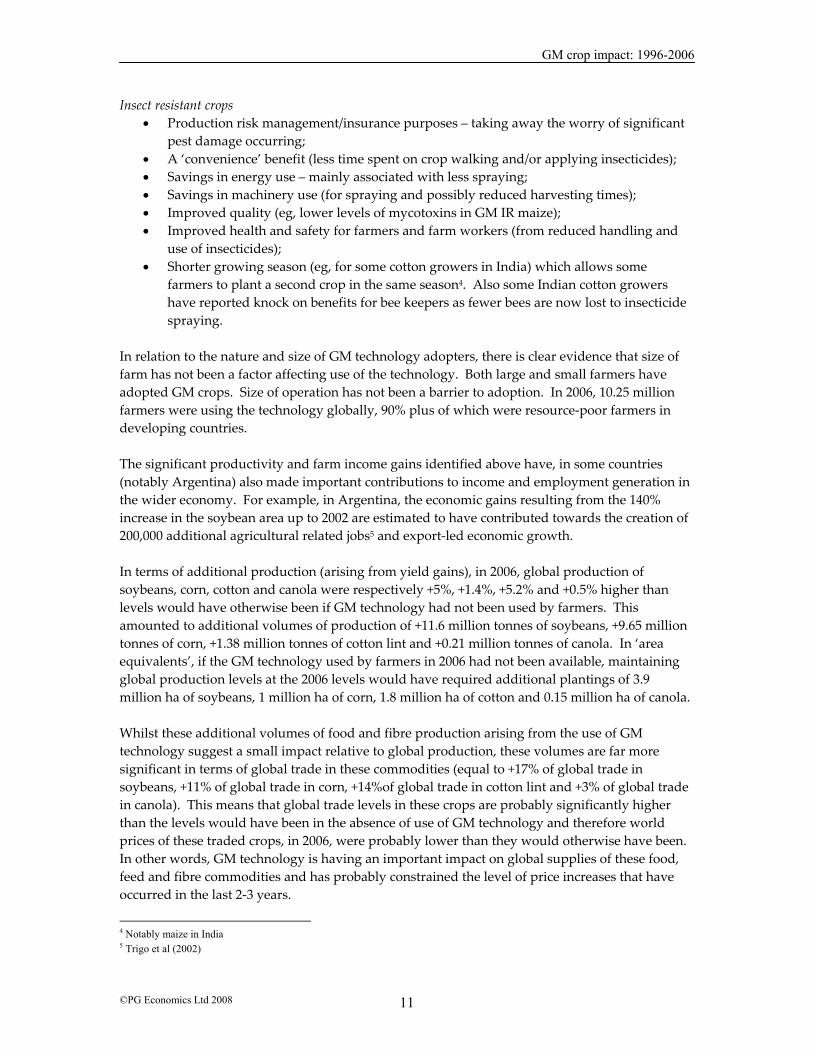
Insect resistant crops • Production risk management/insurance purposes – taking away the worry of significant
pest damage occurring; • A ‘convenience’ benefit (less time spent on crop walking and/or applying insecticides); • Savings in energy use – mainly associated with less spraying; • Savings in machinery use (for spraying and possibly reduced harvesting times); • Improved quality (eg, lower levels of mycotoxins in GM IR maize); • Improved health and safety for farmers and farm workers (from reduced handling and
use of insecticides); • Shorter growing season (eg, for some cotton growers in India) which allows some
farmers to plant a second crop in the same season4. Also some Indian cotton growers have reported knock on benefits for bee keepers as fewer bees are now lost to insecticide spraying.
In relation to the nature and size of GM technology adopters, there is clear evidence that size of farm has not been a factor affecting use of the technology. Both large and small farmers have adopted GM crops. Size of operation has not been a barrier to adoption. In 2006, 10.25 million farmers were using the technology globally, 90% plus of which were resource-poor farmers in developing countries. The significant productivity and farm income gains identified above have, in some countries (notably Argentina) also made important contributions to income and employment generation in the wider economy. For example, in Argentina, the economic gains resulting from the 140% increase in the soybean area up to 2002 are estimated to have contributed towards the creation of 200,000 additional agricultural related jobs5 and export-led economic growth.
In terms of additional production (arising from yield gains), in 2006, global production of soybeans, corn, cotton and canola were respectively +5%, +1.4%, +5.2% and +0.5% higher than levels would have otherwise been if GM technology had not been used by farmers. This amounted to additional volumes of production of +11.6 million tonnes of soybeans, +9.65 million tonnes of corn, +1.38 million tonnes of cotton lint and +0.21 million tonnes of canola. In ‘area equivalents’, if the GM technology used by farmers in 2006 had not been available, maintaining global production levels at the 2006 levels would have required additional plantings of 3.9 million ha of soybeans, 1 million ha of corn, 1.8 million ha of cotton and 0.15 million ha of canola. Whilst these additional volumes of food and fibre production arising from the use of GM technology suggest a small impact relative to global production, these volumes are far more significant in terms of global trade in these commodities (equal to +17% of global trade in soybeans, +11% of global trade in corn, +14%of global trade in cotton lint and +3% of global trade in canola). This means that global trade levels in these crops are probably significantly higher than the levels would have been in the absence of use of GM technology and therefore world prices of these traded crops, in 2006, were probably lower than they would otherwise have been. In other words, GM technology is having an important impact on global supplies of these food, feed and fibre commodities and has probably constrained the level of price increases that have occurred in the last 2-3 years.
4 Notably maize in India 5 Trigo et al (2002)

GM crop impact: 1996-2006
©PG Economics Ltd 2008 12
Environmental impact from changes in insecticide and herbicide use6 To examine this impact, the study has analysed both active ingredient use and utilised the indicator known as the Environmental Impact Quotient (EIQ) to assess the broader impact on the environment (plus impact on animal and human health). The EIQ distils the various environmental and health impacts of individual pesticides in different GM and conventional production systems into a single ‘field value per hectare’ and draws on all of the key toxicity and environmental exposure data related to individual products. It therefore provides a consistent and fairly comprehensive measure to contrast and compare the impact of various pesticides on the environment and human health. Readers should however note that the EIQ is an indicator only and does not take into account all environmental issues and impacts. In the analysis of GM HT technology we have assumed that the conventional alternative delivers the same level of weed control as occurs in the GM HT production system. Table 5 summarises the environmental impact over the last ten years and shows that there have been important environmental gains associated with adoption of GM technology. More specifically:
• There has been a 15.4% net reduction in the environmental impact7 on the cropping area devoted to GM crops since 1996. The total volume of active ingredient (ai) applied to crops has also fallen by 7.8%;
• In absolute terms, since 1996, the largest environmental gains have arisen from the adoption of GM HT soybeans. This mainly reflects the (large) share of global GM crop plantings accounted for by GM HT soybeans. The volume of herbicide use is 4.4% lower and the environmental impact 20.4% lower than levels that would have probably arisen if all of this GM crop area had been planted to conventional cultivars. Readers should note that in some countries (notably in South America), the adoption of GM HT technology in soybeans has also coincided with increases in the volume of herbicides used and the environmental impact relative to historic levels. As indicated above, this largely reflects the facilitating role of the GM HT technology in accelerating and maintaining the switch away from conventional tillage to no/low tillage production systems with their inherent environmental benefits. This net increase in the environmental impact should, therefore be placed in the context of the reduced GHG emissions arising from this production system change (see below) and the general dynamics of agricultural production system changes (which the analysis presented above and in Table 5 takes account of);
• Major environmental gains have also been derived from the adoption of GM insect resistant (IR) cotton (the largest gains on a per hectare basis). Since 1996, there has been a 24.6% reduction in the environmental impact, and a 22.9% decrease in the volume of insecticides applied;
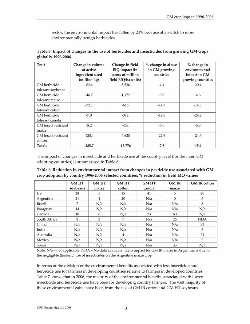
• Important environmental gains have also arisen in the maize and canola sectors. In the maize sector a 5.3% reduction in the environmental impact has occurred from reduced insecticide use and a switch to more environmentally benign herbicides has resulted in a further 4.6% reduction in the environmental impact of maize herbicides. In the canola
6 See section 4.1 7 The actual ai use and the EIQ impact or load in any year has been compared against the likely ai use and EIQ load that would have arisen if the whole crop in any year had been planted to non GM cultivars, using the same tillage system as used in the GM crop and, in the case of crops for which a comparison is made with GM herbicide tolerant crops, delivering the same level of weed control as delivered by the GM production system
GM crop impact: 1996-2006
©PG Economics Ltd 2008 13
sector, the environmental impact has fallen by 24% because of a switch to more environmentally benign herbicides.
Table 5: Impact of changes in the use of herbicides and insecticides from growing GM crops globally 1996-2006
Trait Change in volume of active
ingredient used (million kg)
Change in field EIQ impact (in
terms of million field EIQ/ha units)
% change in ai use in GM growing
countries
% change in environmental impact in GM
growing countries GM herbicide tolerant soybeans
-62.4 -5,536 -4.4 -20.4
GM herbicide tolerant maize
-46.7 -1,172 -3.9 -4.6
GM herbicide tolerant cotton
-32.1 -616 -14.3 -14.5
GM herbicide tolerant canola
-7.9 -372 -12.6 -24.2
GM insect resistant maize
-8.2 -452 -5.0 -5.3
GM insect resistant cotton
-128.4 -5,628 -22.9 -24.6
Totals -285.7 -13,776 -7.8 -15.4 The impact of changes in insecticide and herbicide use at the country level (for the main GM adopting countries) is summarised in Table 6.
Table 6: Reduction in environmental impact from changes in pesticide use associated with GM crop adoption by country 1996-2006 selected countries: % reduction in field EIQ values
GM HT soybeans
GM HT maize
GM HT cotton
GM HT canola
GM IR maize
GM IR cotton
US 28 5 15 41 5 20 Argentina 21 1 20 N/a 0 5 Brazil 7 N/a N/a N/a N/a 8 Paraguay 14 N/a N/a N/a N/a N/a Canada 10 8 N/a 23 60 N/a South Africa 8 2 7 N/a 26 NDA China N/a N/a N/a N/a N/a 33 India N/a N/a N/a N/a N/a 6 Australia N/a N/a 4 N/a N/a 24 Mexico N/a N/a N/a N/a N/a 7 Spain N/a N/a N/a N/a 33 N/a Note: N/a = not applicable, NDA = No data available. Zero impact for GM IR maize in Argentina is due to the negligible (historic) use of insecticides on the Argentine maize crop In terms of the division of the environmental benefits associated with less insecticide and herbicide use for farmers in developing countries relative to farmers in developed countries, Table 7 shows that in 2006, the majority of the environmental benefits associated with lower insecticide and herbicide use have been for developing country farmers. The vast majority of these environmental gains have been from the use of GM IR cotton and GM HT soybeans.

GM crop impact: 1996-2006
©PG Economics Ltd 2008 14
Table 7: GM crop environmental benefits from lower insecticide and herbicide use 2006: developing versus developed countries
% of total reduction in environmental impact: developed
countries
% of total reduction in environmental impact: developing countries
GM HT soybeans 36 64 GM IR maize 94 6 GM HT maize 97 3 GM IR cotton 16 84 GM HT cotton 92 8 GM HT canola 100 0 Total 38 62 Developing countries include all countries in South America Cumulatively over the period 1996 to 2006, developing country farmers have acquired 52% of the total environmental benefits from lower insecticide and herbicide use. Impact on greenhouse gas (GHG) emissions8 The scope for GM crops contributing to lower levels of GHG emissions comes from two principle sources:
• Reduced fuel use from less frequent herbicide or insecticide applications and a reduction in the energy use in soil cultivation. The fuel savings associated with making fewer spray runs (relative to conventional crops) and the switch to conservation, reduced and no-till farming systems, have resulted in permanent savings in carbon dioxide emissions. In 2006 this amounted to about 1,215 million kg (arising from reduced fuel use of 442 million litres). Over the period 1996 to 2006 the cumulative permanent reduction in fuel use is estimated at 5,821 million kg of carbon dioxide (arising from reduced fuel use of 2,120 million litres);
• the use of ‘no-till’ and ‘reduced-till’9 farming systems. These production systems have increased significantly with the adoption of GM HT crops because the GM HT technology has improved growers ability to control competing weeds, reducing the need to rely on soil cultivation and seed-bed preparation as means to getting good levels of weed control. As a result, tractor fuel use for tillage is reduced, soil quality is enhanced and levels of soil erosion cut. In turn more carbon remains in the soil and this leads to lower GHG emissions. Based on savings arising from the rapid adoption of no till/reduced tillage farming systems in North and South America, an extra 3,692 million kg of soil carbon is estimated to have been sequestered in 2006 (equivalent to 13,549 million kg of carbon dioxide that has not been released into the global atmosphere). Cumulatively the amount of carbon sequestered may be higher due to year-on-year benefits to soil quality. However, with only an estimated 15%-25% of the crop area in continuous no-till systems it is currently not possible to confidently estimate cumulative soil sequestration gains.
8 See section 4.2 9 No-till farming means that the ground is not ploughed at all, while reduced tillage means that the ground is disturbed less than it would be with traditional tillage systems. For example, under a no-till farming system, soybean seeds are planted through the organic material that is left over from a previous crop such as corn, cotton or wheat

GM crop impact: 1996-2006
©PG Economics Ltd 2008 15
Placing these carbon sequestration benefits within the context of the carbon emissions from cars, Table 8, shows that:
• In 2006, the permanent carbon dioxide savings from reduced fuel use were the equivalent of removing nearly 0.54 million cars from the road;
• Cumulatively since 1996, the permanent carbon dioxide savings from reduced fuel consumption since the introduction of GM crops are equal to removing 2.58 million cars from the road for one year (9.7% of all registered cars in the UK);
• The additional probable soil carbon sequestration gains in 2006 were equivalent to removing nearly 6.02 million cars from the roads;
• In total, the combined GM crop-related carbon dioxide emission savings from reduced fuel use and additional soil carbon sequestration in 2006 were equal to the removal from the roads of nearly 6.56 million cars, equivalent to about 24.7% of all registered cars in the UK
• It is not possible to confidently estimate the probable soil carbon sequestration gains since 1996 (see above). If the entire GM crop in reduced or no tillage agriculture during the last eleven years had remained in permanent reduced/no tillage then this would have resulted in a carbon dioxide saving of 63.86 billion kg, equivalent to taking 28.4 million cars off the road. This is, however a maximum possibility and the actual levels of carbon dioxide reduction are likely to be lower.
Table 8: Context of carbon sequestration impact 2006: car equivalents
Crop/trait/country Permanent carbon dioxide savings arising from reduced
fuel use (million kg of carbon
dioxide)
Average family car equivalents removed from the road for a year from the
permanent fuel savings
Potential additional soil
carbon sequestration
savings (million kg of carbon
dioxide)
Average family car equivalents removed from the road for a year from the
potential additional soil
carbon sequestration
US: GM HT soybeans 245 108,877 4,064 1,806,345 Argentina: GM HT soybeans
659 293,094 6,994 3,108,408
Other countries: GM HT soybeans
77 34,091 813 361,547
Canada: GM HT canola
136 60,541 1,677 745,304
Global GM IR cotton 98 43,582 0 0
Total 1,215 540,186 13,549 6,021,604 Notes: Assumption: an average family car produces 150 grams of carbon dioxide/km. A car does an average of 15,000 km/year and therefore produces 2,250 kg of carbon dioxide/year

GM crop impact: 1996-2006
©PG Economics Ltd 2008 16
Concluding comments GM technology has, to date delivered several specific agronomic traits that have overcome a number of production constraints for many farmers. This has resulted in improved productivity and profitability for the 10.25 million adopting farmers who have applied the technology to about 100 million hectares in 2006. During the last eleven years, this technology has made important positive socio-economic and environmental contributions. These have arisen even though only a limited range of GM agronomic traits have so far been commercialised, in a small range of crops. The GM technology has delivered economic and environmental gains through a combination of their inherent technical advances and the role of the technology in the facilitation and evolution of more cost effective and environmentally friendly farming practices. More specifically:
• the gains from the GM IR traits have mostly been delivered directly from the technology (yield improvements, reduced production risk and decreased the use of insecticides). Thus farmers (mostly in developing countries) have been able to both improve their productivity and economic returns whilst also practicing more environmentally friendly farming methods;
• the gains from GM HT traits have come from a combination of direct benefits (mostly cost reductions to the farmer) and the facilitation of changes in farming systems. Thus, GM HT technology (especially in soybeans) has played an important role in enabling farmers to capitalise on the availability of a low cost, broad-spectrum herbicide (glyphosate) and in turn, facilitated the move away from conventional to low/no tillage production systems in both North and South America. This change in production system has made additional positive economic contributions to farmers (and the wider economy) and delivered important environmental benefits, notably reduced levels of GHG emissions (from reduced tractor fuel use and additional soil carbon sequestration).
The impact of GM HT traits has, however contributed to increased reliance on a limited range of herbicides and this poses questions about the possible future increased development of weed resistance to these herbicides. Some degree of reduced effectiveness of glyphosate (and glufosinate) against certain weeds is beginning to be found and the extent to which this may develop, will increase the necessity to include low dose rates applications of other herbicides in weed control programmes (commonly used in conventional production systems) and hence may marginally reduce the level of net environmental and economic gains derived from the current use of the GM technology.
GM crop impact: 1996-2006
©PG Economics Ltd 2008 17
1 Introduction 2006 represents the eleventh planting season since genetically modified (GM) crops were first grown in 1996. This study10 examines specific global socio-economics impacts on farm income and environmental impacts in respect of pesticide usage and greenhouse gas (GHG) emissions of the technology over this eleven year period11.
1.1 Objectives The principal objective of the study was to identify the global socio-economic and environmental impact of GM crops over the first eleven years of widespread commercial production. This was to cover not only the impacts for the latest available year but to quantify the cumulative impact over the eleven year period. More specifically, the report examines the following impacts: Socio-economic impacts on:
• Cropping systems: risks of crop losses, use of inputs, crop yields and rotations; • Farm profitability: costs of production, revenue and gross margin profitability; • Trade flows: developments of imports and exports and prices; • Drivers for adoption such as farm type and structure;
Environmental impacts on:
• Insecticide and herbicide use, including conversion to an environmental impact measure12;
• Greenhouse gas (GHG) emissions.
1.2 Methodology The report has been compiled based largely on desk research and analysis. A detailed literature review13 has been undertaken to identify relevant data. Primary data for impacts of commercial cultivation were, of course, not available for every crop, in every year and for each country, but all representative, previous research has been utilised. The findings of this research have been used as the basis for the analysis presented14, although where relevant, primary analysis has been undertaken from base data (eg, calculation of the environmental impacts). More specific information about assumptions used and their origins are provided in each of the sections of the report.
10 The authors acknowledge that funding towards the researching of this paper was provided by Monsanto. The material presented in this paper is, however the independent views of the authors – it is a standard condition for all work undertaken by PG Economics that all reports are independently and objectively compiled without influence from funding sponsors 11 This study updates earlier studies produced in 2005 and 2006, covering the first nine & ten years of GM crop adoption globally. Readers should, however note that some data presented in this report are not directly comparable with data presented in the earlier papers because the current paper takes into account the availability of new data and analysis (including revisions to data applicable to earlier years) 12 The Environmental Impact Quotient (EIQ), based on Kovach J et al (1992 & annually updated) – see references 13 See References 14 Where several pieces of research of relevance to one subject (eg, the impact of using a GM trait on the yield of a crop) have been identified, the findings used have been largely based on the average

GM crop impact: 1996-2006
©PG Economics Ltd 2008 18
1.3 Structure of report The report is structured as follows:
• Section one: introduction • Section two: overview of GM crop plantings by trait and country • Section three: farm level profitability impacts by trait and country, intangible
benefits, structure and size, prices and trade flows; • Section four: environmental impacts covering impact of changes in herbicide and
insecticide use and contributions to reducing GHG emissions.
GM crop impact: 1996-2006
©PG Economics Ltd 2008 19
2 Global context of GM crops This section provides a broad overview of the global development of GM crops over the eleven year period.
2.1 Global plantings Although the first commercial GM crops were planted in 1994 (tomatoes), 1996 was the first year in which a significant area (1.66 million hectares) of crops were planted containing GM traits. Since then there has been a dramatic increase in plantings and by 2006/07, the global planted area reached almost 100 million hectares. This is equal to 62% of the total utilised agricultural area of the European Union (EU 27), twice the EU 27 area devoted to cereals or six times the total agricultural area of the UK. In terms of the share of the main crops in which GM traits have been commercialised (soybeans, corn, cotton and canola), GM traits accounted for 33% of the global plantings to these four crops in 2006.
2.2 Plantings by crop and trait
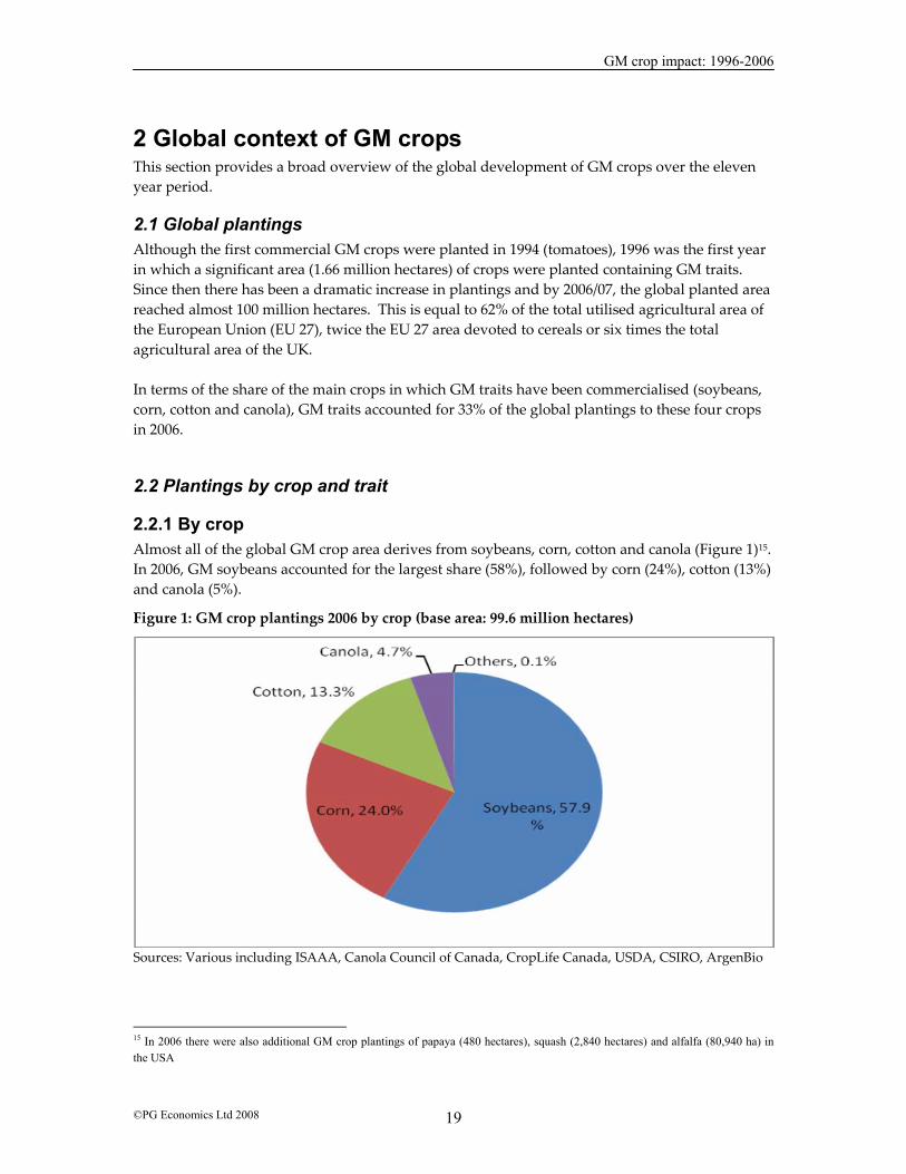
2.2.1 By crop Almost all of the global GM crop area derives from soybeans, corn, cotton and canola (Figure 1)15. In 2006, GM soybeans accounted for the largest share (58%), followed by corn (24%), cotton (13%) and canola (5%).
Figure 1: GM crop plantings 2006 by crop (base area: 99.6 million hectares)
Sources: Various including ISAAA, Canola Council of Canada, CropLife Canada, USDA, CSIRO, ArgenBio
15 In 2006 there were also additional GM crop plantings of papaya (480 hectares), squash (2,840 hectares) and alfalfa (80,940 ha) in the USA

GM crop impact: 1996-2006
©PG Economics Ltd 2008 20
In terms of the share of total global plantings to these four crops, GM traits accounted for a majority of soybean plantings (61.5%) in 2006. For the other three main crops, the GM shares in 2006 were 16.2% for corn, 38.4% for cotton and 17.5% for canola (Figure 2).
Figure 2: 2006’s share of GM crops in global plantings of key crops (hectares)
Sources: Various including ISAAA, Canola Council of Canada, CropLife Canada, USDA, CSIRO, ArgenBio The trend in plantings to GM crops (by crop) since 1996 is shown in Figure 3.
Figure 3: Global GM crop plantings by crop 1996-2006 (hectares)
Sources: Various including ISAAA, Canola Council of Canada, CropLife Canada, USDA, CSIRO, ArgenBio
2.2.2 By trait Figure 4 summarises the breakdown of the main GM traits planted globally in 2006. GM herbicide tolerant soybeans dominate accounting for 54% of the total followed by insect resistant

GM crop impact: 1996-2006
©PG Economics Ltd 2008 21
(largely Bt) corn, herbicide tolerant corn and insect resistant cotton with respective shares of 15%, 12% and 11%16. In total, herbicide tolerant crops account for 74%, and insect resistant crops account for 26% of global plantings.
Figure 4: Global GM crop plantings by main trait and crop: 2006
Sources: Various including ISAAA, Canola Council of Canada, CropLife Canada, USDA, CSIRO, ArgenBio
2.2.3 By country The US had the largest share of global GM crop plantings in 2006 (52%: 52.1 million ha), followed by Argentina (18.4 million ha: 18% of the global total). The other main countries planting GM crops in 2006 were Canada, Brazil, India and China (Figure 5).
Figure 5: Global GM crop plantings 2006 by country
Sources: Various including ISAAA, Canola Council of Canada, CropLife Canada, USDA, CSIRO, ArgenBio
16 The reader should note that the total plantings by trait produces a higher global planted area (107.1 million ha) than the global area by crop (99.6 million ha) because of the planting of some crops containing the stacked traits of herbicide tolerance and insect resistance

GM crop impact: 1996-2006
©PG Economics Ltd 2008 22
Table 9 shows the trends in GM crop plantings by country since 1996. This again highlights the importance of countries like the US, Canada, Brazil, China and Argentina both in current planting terms and as early adopters of the technology. More recently, significant and increasing areas have been planted to GM crops in newer adopting countries such as Paraguay, South Africa and India (and other countries such as Spain, Romania, the Philippines, Mexico and Uruguay).
Table 9: Global GM plantings by country 1996-2006 (‘000 hectares)
Country 1996 1997 1998 1999 2000 2001 2002 2003 2004 2005 2006 USA 1,449 7,460 19,259 26,252 28,245 33,024 37,528 40,723 44,788 47,395 52,081 Canada 139 648 2,161 3,529 3,331 3,212 3,254 4,427 5,074 5,858 5,921 Argentina 37 1,756 4,818 6,844 9,605 11,775 13,587 14,895 15,883 16,930 18,423 Brazil 0 100 500 1,180 1,300 1,311 1,742 3,000 5,000 9,000 11,758 China 0 34 261 654 1,216 2,174 2,100 2,800 3,700 3,300 3,612 Paraguay 0 0 0 58 94 338 477 737 1,200 1,800 1,928 Australia 40 58 100 133 185 204 162 165 248 275 139 South Africa
0 0 0.08 0.75 93 150 214 301 528 595 1,418
India 0 0 0 0 0 0 44 100 500 1,300 3,800 Others 0.9 15 62 71 94 112 136 209 527 710 522 Total 1,665 10,072 27,161 38,730 44,163 52,300 59,245 67,357 77,448 87,163 99,602 Sources: Various including ISAAA, Canola Council of Canada, CropLife Canada, USDA, CSIRO, ArgenBio Within the leading countries, the breakdown of the GM crop plantings in 2006 was as follows:
• The US: the main GM crops were soybeans and corn which accounted for 52% and 37% respectively of total GM plantings in the US . The balance came from cotton (10%) and canola (1%);
• Canada: canola dominated GM plantings with a 72% share. The balance was roughly equally split between corn (15%) and soybeans (13%);
• Argentina: soybeans accounted for the vast bulk of GM crop plantings (86%), followed by corn (12%) and cotton (2%);
• In Brazil plantings are dominated by soybeans (97%), followed by cotton (3%); • In China, India and Australia all plantings were cotton.
In terms of the GM share of production in the main GM technology adopting countries, Table 10 shows that, in 2006, GM technology accounted for important shares of total production of the four main crops, in several countries. GM cultivars have been adopted at unprecedented rates by both small and large growers because the novel traits provide cost effective options for growers to exploit (eg, reducing expenditure on herbicides and insecticides).
Table 10: GM technology share of crop plantings in 2006 by country (% of total plantings)
Soybeans Maize Cotton Canola USA 89 61 83 98 Canada 63 67 N/a 84 Argentina 98 80 79 N/a

GM crop impact: 1996-2006
©PG Economics Ltd 2008 23
South Africa 70 43 47 N/a Australia N/a N/a 93 N/a China N/a N/a 65 N/a Paraguay 90 N/a N/a N/a Brazil 55 N/a 13 N/a Uruguay 100 44 N/a N/a Note: N/a = not applicable
GM crop impact: 1996-2006
©PG Economics Ltd 2008 24
3 The farm level economic impact of GM crops 1996-2006 This section examines the farm level economic impact of growing GM crops and covers the following main issues:
• Impact on crop yields; • Effect on key costs of production, notably seed cost and crop protection expenditure; • Impact on other costs such as fuel and labour; • Effect on profitability; • Other impacts such as crop quality, scope for planting a second crop in a season and
impacts that are often referred to as intangible impacts such as convenience, risk management and husbandry flexibility.
As indicated in the introduction, the primary methodology has been to review existing literature and to use the findings as the basis for the impact estimates over the eleven year period examined. Additional points to note include:
• All values shown are nominal (for the year shown); • Actual average prices and yields are used for each year; • The base currency used is the US dollar. All financial impacts identified in other
currencies have been converted to US dollars at the prevailing annual average exchange rate for each year;
• Where yield impacts have been identified in studies for one or a limited number of years, these have been converted into a percentage change impact and applied to all other years on the basis of the prevailing average yield recorded. For example, if a study identified a yield gain of 5% on a base yield of 10 tonnes/ha in year one, this 5% yield increase was then applied to the average yield recorded in each other year17.
The section is structured on a trait and country basis highlighting the key farm level impacts.
3.1 Herbicide tolerant soybeans
3.1.1 The US In 2006, 89% of the total US soybean crop was planted to GM glyphosate tolerant cultivars (GM HT). The farm level impact of using this technology since 1996 is summarised in Table 11. The key features are as follows:
• The primary impact has been to reduce the soybean cost of production. In the early years of adoption these savings were between $25/ha and $34/ha. In more recent years, estimates of the cost savings have risen to between $60/ha and $78/ha (based on a comparison of conventional herbicide regimes in the early 2000s that would be required to deliver a comparable level of weed control to the GM HT soybean system). The main
17 The average base yield has been adjusted downwards (if necessary) to take account of any positive yield impact of the technology. In this way the impact on total production of any yield gains is not overstated

GM crop impact: 1996-2006
©PG Economics Ltd 2008 25
savings have come from lower herbicide costs18 plus a $6/ha to $10/ha savings in labour and machinery costs;
• Against the background of underlying improvements in average yield levels over the 1996-2006 period (via improvements in plant breeding), the specific yield impact of the GM HT technology used up to 2006 has been neutral19;
• The annual total national farm income benefit from using the technology has risen from $5 million in 1996 to over $1.2 billion in 2006. The cumulative farm income benefit over the 1996-2006 period (in nominal terms) was $8.73 billion;
• In added value terms, the increase in farm income in recent years has been equivalent to an annual increase in production of between +5% and +10%.
Table 11: Farm level income impact of using GM HT soybeans in the US 1996-2006
Year Cost savings ($/ha)
Net cost saving/increase in gross margins, inclusive of cost of technology ($/ha)
Increase in farm income at a national level ($ millions)
Increase in national farm income as % of farm level value of national production
1996 25.2 10.39 5.0 0.03 1997 25.2 10.39 33.2 0.19 1998 33.9 19.03 224.1 1.62 1999 33.9 19.03 311.9 2.5 2000 33.9 19.03 346.6 2.69 2001 73.4 58.56 1,298.5 10.11 2002 73.4 58.56 1,421.7 9.53 2003 78.5 61.19 1,574.9 9.57 2004 60.1 40.33 1,096.8 4.57 2005 69.4 44.71 1,201.4 6.87 2006 69.4 44.71 1,216.2 5.89 Sources and notes:
1. Impact data 1996-1997 based on Marra et al, 1998-2000 based on Gianessi & Carpenter and 2001 onwards based on NCFAP (2003 & 2006)
2. Cost of technology: $14.82/ha 1996-2002, $17.3/ha 2003, $19.77/ha 2004, $24.71/ha 2005 onwards 3. The higher values for the cost savings in 2001 onwards reflect the methodology used by NCFAP
which was to examine the conventional herbicide regime that would be required to deliver the same level of weed control in a low/reduced till system to that delivered from the GM HT no/reduced till soybean system. This is a more robust methodology than some of the more simplistic alternatives (eg, Benbrook, 2003) used elsewhere. In earlier years the cost savings were based on comparisons between GM HT soy growers and/or conventional herbicide regimes that were commonplace prior to commercialisation in the mid 1990s when conventional tillage systems were more important
18 Whilst there were initial cost savings in herbicide expenditure, these increased when glyphosate came off-patent in 2000. Growers of GM HT soybeans initially applied Monsanto’s Roundup herbicide but over time, and with the availability of low cost generic glyphosate alternatives, many growers (eg, estimated at 30% by 2005) switched to using these generic alternatives (the price of Roundup also fell significantly post 2000) 19 Some early studies of the impact of GM HT soybeans in the US, suggested that GM HT soybeans produced lower yields than conventional soybean varieties. Where this may have occurred it applied only in early years of adoption when the technology was not present in all leading varieties suitable for all of the main growing regions of the USA. By 1998/99 the technology was available in leading varieties and no statistically significant average yield differences have been found between GM and conventional soybean varieties

GM crop impact: 1996-2006
©PG Economics Ltd 2008 26
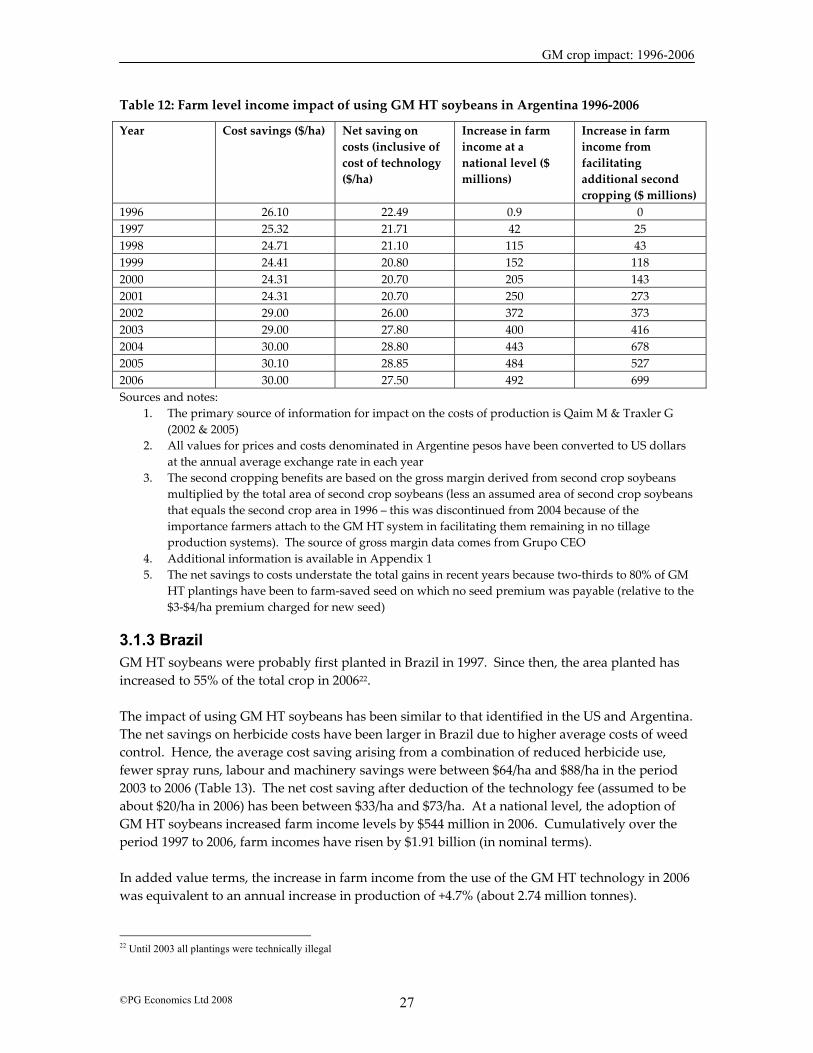
3.1.2 Argentina As in the US, GM HT soybeans were first planted commercially in 1996. Since then use of the technology has increased rapidly, so that by the early 2000s, almost all soybeans grown in Argentina were GM HT (98%). Not surprisingly the impact on farm income has been substantial, with farmers deriving important cost saving and farm income benefits both similar and additional to those obtained in the US (Table 12). More specifically:
• The impact on yield has been neutral (ie, no positive or negative yield impact); • The cost of the technology to Argentine farmers has been substantially lower than in the
US (about $1-$4/hectare compared to $15-$25/ha in the US) mainly because the main technology provider (Monsanto) was not able to obtain patent protection for the technology in Argentina. As such, Argentine farmers have been free to save and use GM seed without paying any technology fees or royalties (on farm-saved seed) for many years and estimates of the proportion of total soybean seed used that derives from a combination of declared saved seed and uncertified seed in 2006 were about 75% (ie, 25% of the crop was planted to certified seed);
• The savings from reduced expenditure on herbicides, fewer spray runs and machinery use have been in the range of $24-$30/ha, resulting in a net income gain of $21-$29/ha20;
• The price received by farmers for GM HT soybeans was on average marginally higher than for conventionally produced soybeans because of lower levels of weed material and impurities in the crop. This quality premia was equivalent to about 0.5% of the baseline price for soybeans;
• The net income gain from use of the GM HT technology at a national level was $492 million in 2006. Since 1996, the cumulative benefit (in nominal terms) has been $2.96 billion;
• An additional farm income benefit that many Argentine soybean growers have derived comes from the additional scope for second cropping of soybeans. This has arisen because of the simplicity, ease and weed management flexibility provided by the (GM) technology which has been an important factor facilitating the use of no and reduced tillage production systems. In turn the adoption of low/no tillage production systems has reduced the time required for harvesting and drilling subsequent crops and hence has enabled many Argentine farmers to cultivate two crops (wheat followed by soybeans) in one season. As such, 20% of the total Argentine soybean crop was second crop in 200621, compared to 8% in 1996. Based on the additional gross margin income derived from second crop soybeans (see Appendix 1), this has contributed a further boost to national soybean farm income of $699 million in 2006 and $3.29 billion cumulatively since 1996;
• The total farm income benefit inclusive of the second cropping was $1.19 billion in 2006 and $6.25 billion cumulatively between 1996 and 2006;
• In added value terms, the increase in farm income from the direct use of the GM HT technology (ie, excluding the second crop benefits) in last three years has been equivalent to an annual increase in production of between +4% and +6%. The additional production from second soybean cropping facilitated by the technology in 2006 was equal to 20% of total output.
20 This income gain also includes the benefits accruing from the fall in real price of glyphosate, which fell by about a third between 1996 and 2000 21 The second crop share was 3.2 million ha in 2006
GM crop impact: 1996-2006
©PG Economics Ltd 2008 27
Table 12: Farm level income impact of using GM HT soybeans in Argentina 1996-2006
Year Cost savings ($/ha) Net saving on costs (inclusive of cost of technology ($/ha)
Increase in farm income at a national level ($ millions)
Increase in farm income from facilitating additional second cropping ($ millions)
1996 26.10 22.49 0.9 0 1997 25.32 21.71 42 25 1998 24.71 21.10 115 43 1999 24.41 20.80 152 118 2000 24.31 20.70 205 143 2001 24.31 20.70 250 273 2002 29.00 26.00 372 373 2003 29.00 27.80 400 416 2004 30.00 28.80 443 678 2005 30.10 28.85 484 527 2006 30.00 27.50 492 699 Sources and notes:
1. The primary source of information for impact on the costs of production is Qaim M & Traxler G (2002 & 2005)
2. All values for prices and costs denominated in Argentine pesos have been converted to US dollars at the annual average exchange rate in each year
3. The second cropping benefits are based on the gross margin derived from second crop soybeans multiplied by the total area of second crop soybeans (less an assumed area of second crop soybeans that equals the second crop area in 1996 – this was discontinued from 2004 because of the importance farmers attach to the GM HT system in facilitating them remaining in no tillage production systems). The source of gross margin data comes from Grupo CEO
4. Additional information is available in Appendix 1 5. The net savings to costs understate the total gains in recent years because two-thirds to 80% of GM
HT plantings have been to farm-saved seed on which no seed premium was payable (relative to the $3-$4/ha premium charged for new seed)
3.1.3 Brazil GM HT soybeans were probably first planted in Brazil in 1997. Since then, the area planted has increased to 55% of the total crop in 200622. The impact of using GM HT soybeans has been similar to that identified in the US and Argentina. The net savings on herbicide costs have been larger in Brazil due to higher average costs of weed control. Hence, the average cost saving arising from a combination of reduced herbicide use, fewer spray runs, labour and machinery savings were between $64/ha and $88/ha in the period 2003 to 2006 (Table 13). The net cost saving after deduction of the technology fee (assumed to be about $20/ha in 2006) has been between $33/ha and $73/ha. At a national level, the adoption of GM HT soybeans increased farm income levels by $544 million in 2006. Cumulatively over the period 1997 to 2006, farm incomes have risen by $1.91 billion (in nominal terms). In added value terms, the increase in farm income from the use of the GM HT technology in 2006 was equivalent to an annual increase in production of +4.7% (about 2.74 million tonnes). 22 Until 2003 all plantings were technically illegal

GM crop impact: 1996-2006
©PG Economics Ltd 2008 28
Table 13: Farm level income impact of using GM HT soybeans in Brazil 1997-2006
Year Cost savings ($/ha) Net cost saving after inclusion of technology cost ($/ha)
Impact on farm income at a national level ($ millions)
Increase in national farm income as % of farm level value of national production
1997 38.8 35.19 3.8 0.06 1998 42.12 38.51 20.5 0.31 1999 38.76 35.15 43.5 0.96 2000 65.32 31.71 43.7 0.85 2001 46.32 42.71 58.7 1.02 2002 40.00 36.39 66.7 1.07 2003 77.00 68.00 214.7 1.62 2004 88.00 73.00 377.6 3.47 2005 73.60 57.43 538.4 4.98 2006 64.73 44.96 544.1 4.71 Sources and notes:
1. Impact data based on 2004 comparison data from the Parana Department of Agriculture (2004) Cost of production comparison: biotech and conventional soybeans, in USDA GAIN report BR4629 of 11 November 2004. www.fas.usad.gov/gainfiles/200411/146118108.pdf
2. Cost of the technology from 2003 is based on the royalty payments officially levied by the technology providers. For years up to 2002, the cost of technology is based on costs of buying new seed in Argentina (the source of the seed). This probably overstates the real cost of the technology and understates the cost savings
3. All values for prices and costs denominated in Brazilian Real have been converted to US dollars at the annual average exchange rate in each year
3.1.4 Paraguay and Uruguay GM HT soybeans have been grown since 1999 and 2000 respectively in Paraguay and Uruguay. By 2006, they accounted for 90% of total soybean plantings in Paraguay and all of the soybean plantings in Uruguay23. Using the farm level impact data derived from Argentine research and applying this to production in these two countries24, Figure 6 summarises the national farm level income benefits that have been derived from using the technology. In 2006, the respective national farm income gains were $49.7 million in Paraguay and $8.8 million in Uruguay.
23 As in Argentina, the majority of plantings are to farm saved or uncertified seed. For example, 64% of plantings in Paraguay in 2006 were estimated to be uncertified seed 24 Quam & Traxler (2002 & 2005). The authors are not aware of any specific impact research having been conducted and published in Paraguay or Uruguay
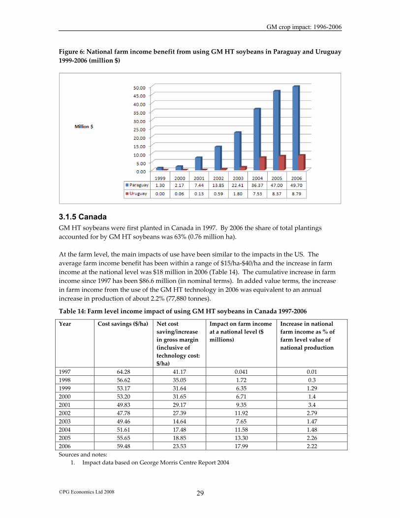
GM crop impact: 1996-2006
©PG Economics Ltd 2008 29
Figure 6: National farm income benefit from using GM HT soybeans in Paraguay and Uruguay 1999-2006 (million $)
3.1.5 Canada GM HT soybeans were first planted in Canada in 1997. By 2006 the share of total plantings accounted for by GM HT soybeans was 63% (0.76 million ha). At the farm level, the main impacts of use have been similar to the impacts in the US. The average farm income benefit has been within a range of $15/ha-$40/ha and the increase in farm income at the national level was $18 million in 2006 (Table 14). The cumulative increase in farm income since 1997 has been $86.6 million (in nominal terms). In added value terms, the increase in farm income from the use of the GM HT technology in 2006 was equivalent to an annual increase in production of about 2.2% (77,880 tonnes).
Table 14: Farm level income impact of using GM HT soybeans in Canada 1997-2006
Year Cost savings ($/ha) Net cost saving/increase in gross margin (inclusive of technology cost: $/ha)
Impact on farm income at a national level ($ millions)
Increase in national farm income as % of farm level value of national production
1997 64.28 41.17 0.041 0.01 1998 56.62 35.05 1.72 0.3 1999 53.17 31.64 6.35 1.29 2000 53.20 31.65 6.71 1.4 2001 49.83 29.17 9.35 3.4 2002 47.78 27.39 11.92 2.79 2003 49.46 14.64 7.65 1.47 2004 51.61 17.48 11.58 1.48 2005 55.65 18.85 13.30 2.26 2006 59.48 23.53 17.99 2.22 Sources and notes:
1. Impact data based on George Morris Centre Report 2004

GM crop impact: 1996-2006
©PG Economics Ltd 2008 30
2. All values for prices and costs denominated in Canadian dollars have been converted to US dollars at the annual average exchange rate in each year
3.1.6 South Africa The first year GM HT soybeans were planted commercially in South Africa was 2001. By 2006, 150,000 hectares (70%) of total soybean plantings were to varieties containing the GM HT trait. In terms of impact at the farm level, net cost savings of between $5/ha and $9/ha have been achieved through reduced expenditure on herbicides (Table 15). At the national level, the increase in farm income was $0.78 million in 2006. Cumulatively the farm income gain since 2001 has been $3 million.
Table 15: Farm level income impact of using GM HT soybeans in South Africa 2001-2006
Year Cost savings ($/ha) Net cost saving/increase in gross margin after inclusion of technology cost ($/ha)
Impact on farm income at a national level ($ millions)
2001 26.72 7.02 0.042 2002 21.82 5.72 0.097 2003 30.40 7.90 0.24 2004 34.94 9.14 0.46 2005 36.17 9.12 1.42 2006 33.96 5.17 0.78 Sources and notes:
1. Impact data (source: Monsanto South Africa) 2. All values for prices and costs denominated in South African Rand have been converted to US
dollars at the annual average exchange rate in each year
3.1.7 Romania In 2006, Romania planted 130,000 ha of GM HT soybeans (total soybean area 191,000 ha). This was its eighth year of commercial use of the technology. The growing of GM HT soybeans in Romania has resulted in substantially greater net farm income gains per hectare than any of the other countries using the technology:
• Yield gains of an average of 31%25 have been recorded. This yield gain has arisen from the substantial improvements in weed control26;
• The cost of the technology to farmers in Romania has tended to be higher than other countries, with seed being sold in conjunction with the herbicide. For example, in the last four years, the average cost of seed and herbicide per hectare was $120/ha to $130/ha. This relatively high cost however, has not deterred adoption of the technology because of the major yield gains, improvements in the quality of soybeans produced
25 Source: Brookes (2005) 26 Weed infestation levels, particularly of difficult to control weeds such as Johnson grass have been very high in Romania. This is largely a legacy of the economic transition during the 1990s which resulted in very low levels of farm income, abandonment of land and very low levels of weed control. As a result, the weed bank developed substantially and has been subsequently very difficult to control, until the GM HT soybean system became available (glyphosate has been the key to controlling difficult weeds like Johnson grass)
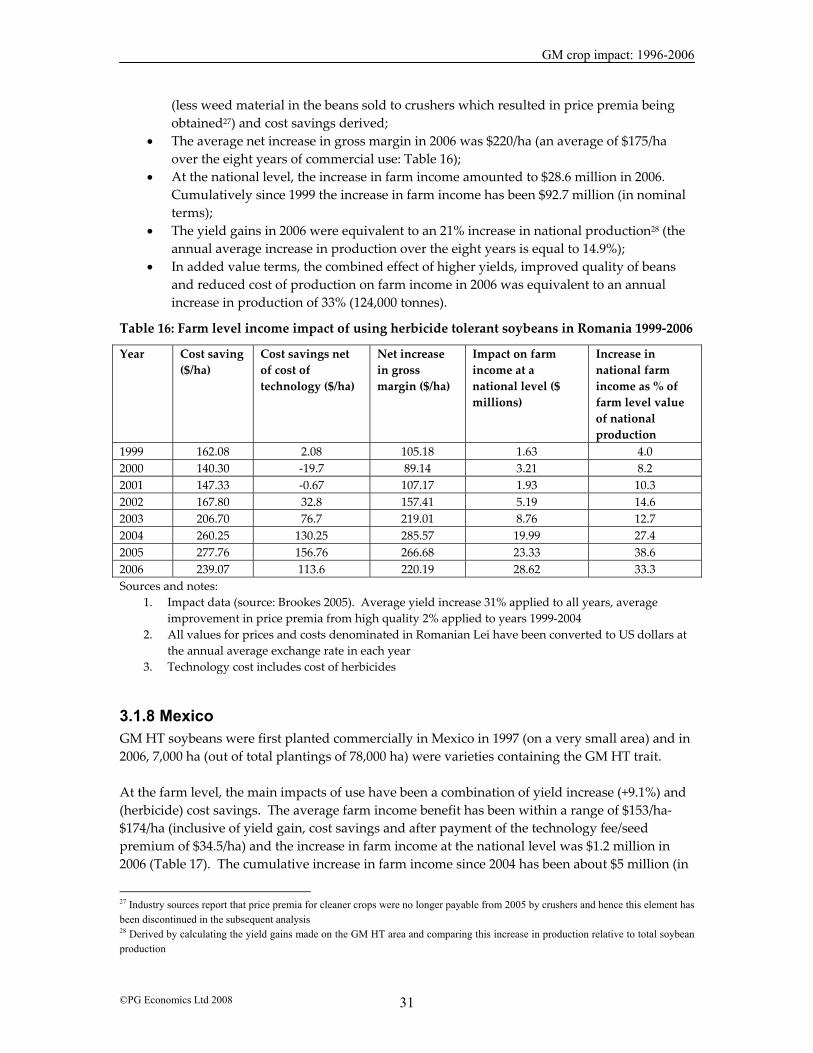
GM crop impact: 1996-2006
©PG Economics Ltd 2008 31
(less weed material in the beans sold to crushers which resulted in price premia being obtained27) and cost savings derived;
• The average net increase in gross margin in 2006 was $220/ha (an average of $175/ha over the eight years of commercial use: Table 16);
• At the national level, the increase in farm income amounted to $28.6 million in 2006. Cumulatively since 1999 the increase in farm income has been $92.7 million (in nominal terms);
• The yield gains in 2006 were equivalent to an 21% increase in national production28 (the annual average increase in production over the eight years is equal to 14.9%);
• In added value terms, the combined effect of higher yields, improved quality of beans and reduced cost of production on farm income in 2006 was equivalent to an annual increase in production of 33% (124,000 tonnes).
Table 16: Farm level income impact of using herbicide tolerant soybeans in Romania 1999-2006
Year Cost saving ($/ha)
Cost savings net of cost of technology ($/ha)
Net increase in gross margin ($/ha)
Impact on farm income at a national level ($ millions)
Increase in national farm income as % of farm level value of national production
1999 162.08 2.08 105.18 1.63 4.0 2000 140.30 -19.7 89.14 3.21 8.2 2001 147.33 -0.67 107.17 1.93 10.3 2002 167.80 32.8 157.41 5.19 14.6 2003 206.70 76.7 219.01 8.76 12.7 2004 260.25 130.25 285.57 19.99 27.4 2005 277.76 156.76 266.68 23.33 38.6 2006 239.07 113.6 220.19 28.62 33.3 Sources and notes:
1. Impact data (source: Brookes 2005). Average yield increase 31% applied to all years, average improvement in price premia from high quality 2% applied to years 1999-2004
2. All values for prices and costs denominated in Romanian Lei have been converted to US dollars at the annual average exchange rate in each year
3. Technology cost includes cost of herbicides
3.1.8 Mexico GM HT soybeans were first planted commercially in Mexico in 1997 (on a very small area) and in 2006, 7,000 ha (out of total plantings of 78,000 ha) were varieties containing the GM HT trait. At the farm level, the main impacts of use have been a combination of yield increase (+9.1%) and (herbicide) cost savings. The average farm income benefit has been within a range of $153/ha-$174/ha (inclusive of yield gain, cost savings and after payment of the technology fee/seed premium of $34.5/ha) and the increase in farm income at the national level was $1.2 million in 2006 (Table 17). The cumulative increase in farm income since 2004 has been about $5 million (in
27 Industry sources report that price premia for cleaner crops were no longer payable from 2005 by crushers and hence this element has been discontinued in the subsequent analysis 28 Derived by calculating the yield gains made on the GM HT area and comparing this increase in production relative to total soybean production

GM crop impact: 1996-2006
©PG Economics Ltd 2008 32
nominal terms). In added value terms, the increase in farm income from the use of the GM HT technology in 2006 was equivalent to an annual increase in production of about 2.4% (4,400 tonnes).
Table 17: Farm level income impact of using GM HT soybeans in Mexico 2004-2006
Year Cost savings ($/ha) Net cost saving/increase in gross margin (inclusive of technology cost & yield gain: $/ha)
Impact on farm income at a national level ($ millions)
Increase in national farm income as % of farm level value of national production
2004 154.5 152.90 2,17 6.3 2005 154.5 158.21 1,67 3.8 2006 154.5 174.45 1,21 2.4 Sources and notes:
1. Impact data based on Monsanto, 2007. Reporte final del programa Soya Solución Faena en Chiapas. Monsanto Comercial
2. All values for prices and costs denominated in Mexican pesos have been converted to US dollars at the annual average exchange rate in each year
3.1.9 Summary of global economic impact In global terms, the farm level impact of using GM HT technology in soybeans was $2.36 billion in 2006 (Figure 7). If the second crop benefits arising in Argentina are included this rises to $3.1 billion. Cumulatively since 1996, the farm income benefit has been (in nominal terms) $14 billion ($17.45 billion if second crop gains in Argentina and Paraguay are included). In terms of the total value of soybean production from the countries growing GM HT soybeans in 2006, the additional farm income (inclusive of Argentine second crop gains) generated by the technology is equal to a value added equivalent of 6.74%. Relative to the value of global soybean production in 2006, the farm income benefit added the equivalent of 5.6%. These economic benefits should be placed within the context of a significant increase in the level of soybean production in the main GM adopting countries since 1996 (a 60% increase in the area planted in the leading soybean producing countries of the US, Brazil and Argentina).

GM crop impact: 1996-2006
©PG Economics Ltd 2008 33
Figure 7: Global farm level income benefits derived from using GM HT soybeans 1996-2006 (million $)
These economic benefits mostly derive from cost savings although farmers in Mexico and Romania also obtained yield gains (from significant improvements in weed control levels relative to levels applicable prior to the introduction of the technology). If it is also assumed that all of the second crop soybean gains are effectively additional production that would not have otherwise occurred without the GM HT technology (the GM HT technology facilitated major expansion of second crop soybeans in Argentina and to a lesser extent in Paraguay) then these gains are de facto ʹyieldʹ gains. Under this assumption, of the total cumulative farm income gains from using GM HT soy ($17.45 billion), $3.5 billion (20%) is due to yield gains and the balance, 80% is due to cost savings.
3.2 Herbicide tolerant maize
3.2.1 The US Herbicide tolerant maize29 has been used commercially in the US since 1997 and by 2006 was planted on 36% of the total US maize crop. The impact of using this technology at the farm level is summarised in Figure 8. As with herbicide tolerant soybeans, the main benefit has been to reduce costs, and hence improve profitability levels. Average profitability improved by $23/ha- $25/ha, resulting in a net gain to farm income in 2006 of $268 million. Cumulatively, since 1997 the farm income benefit has been $1.05 billion. In added value terms, the effect of reduced costs of production on farm income in 2006 was equivalent to an annual increase in production of 0.72% (2.24 million tonnes).
29 Tolerant to glufosinate ammonium or to glyphosate, although cultivars tolerant to glyphosate has accounted for the majority of plantings
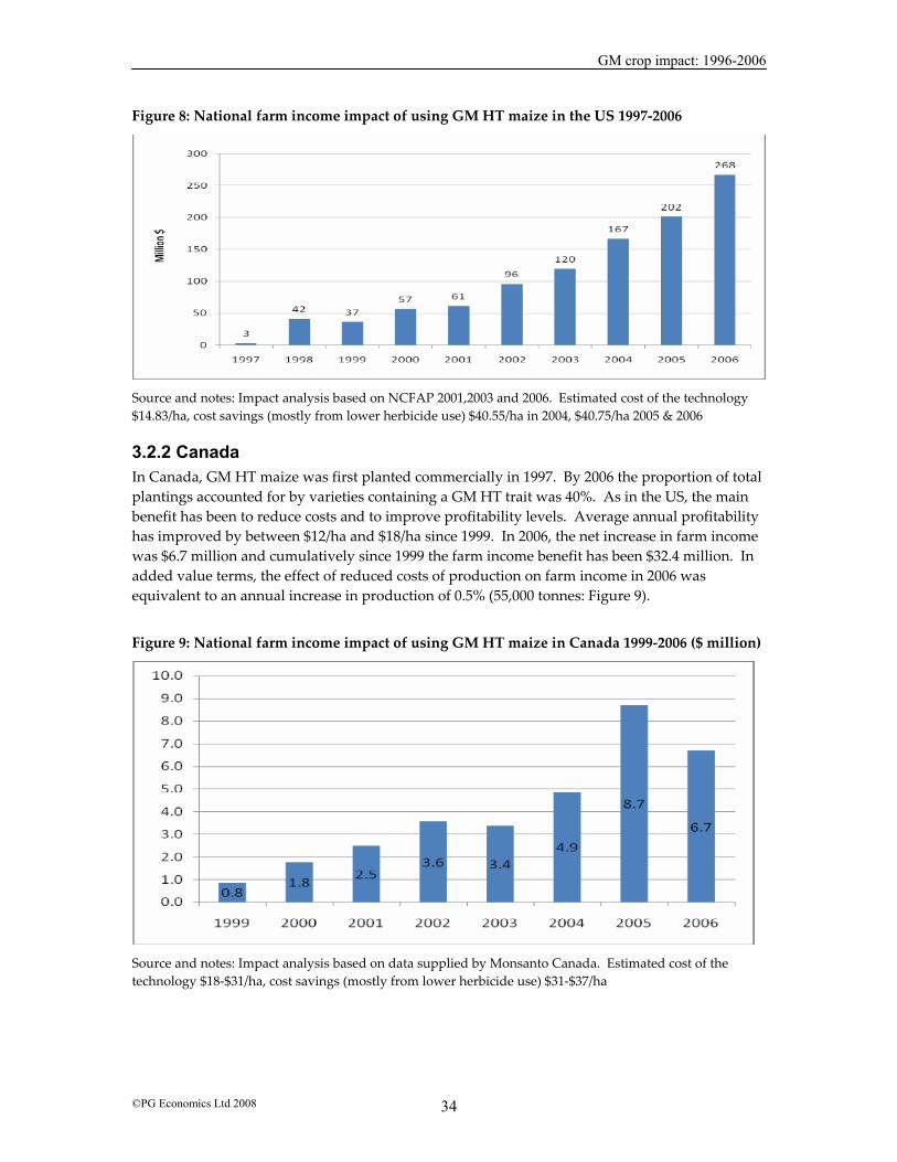
GM crop impact: 1996-2006
©PG Economics Ltd 2008 34
Figure 8: National farm income impact of using GM HT maize in the US 1997-2006
Source and notes: Impact analysis based on NCFAP 2001,2003 and 2006. Estimated cost of the technology $14.83/ha, cost savings (mostly from lower herbicide use) $40.55/ha in 2004, $40.75/ha 2005 & 2006
3.2.2 Canada In Canada, GM HT maize was first planted commercially in 1997. By 2006 the proportion of total plantings accounted for by varieties containing a GM HT trait was 40%. As in the US, the main benefit has been to reduce costs and to improve profitability levels. Average annual profitability has improved by between $12/ha and $18/ha since 1999. In 2006, the net increase in farm income was $6.7 million and cumulatively since 1999 the farm income benefit has been $32.4 million. In added value terms, the effect of reduced costs of production on farm income in 2006 was equivalent to an annual increase in production of 0.5% (55,000 tonnes: Figure 9).
Figure 9: National farm income impact of using GM HT maize in Canada 1999-2006 ($ million)
Source and notes: Impact analysis based on data supplied by Monsanto Canada. Estimated cost of the technology $18-$31/ha, cost savings (mostly from lower herbicide use) $31-$37/ha

GM crop impact: 1996-2006
©PG Economics Ltd 2008 35
3.2.3 Argentina GM HT maize was first planted commercially in Argentina in 2004 (217,000 ha in 2006). It has been adopted in two distinct types of area, the majority (80%) in the traditional ‘corn production belt’ and 20% in newer maize-growing regions, which have been traditionally known as more marginal areas that surround the ‘Corn Belt’ (20% of adoption in 2006). The limited adoption of GM HT technology in Argentina up to 2006 was mainly due to the technology only being available as a single gene, not stacked with the GM IR (bt) trait, which most maize growers have also adopted. Hence, faced with an either GM HT or GM IR trait available for use, most farmers have chosen the GM IR trait because the additional returns derived from adoption have tended to be (on average) greater from the GM IR trait than the GM HT trait (see below for further details of returns from the GM HT trait). In relation to impact on farm income:
• In all regions the cost of the technology (about $20/ha) has been broadly equal to the saving in herbicide costs;
• In the Corn Belt area, use of the technology has resulted in an average 3% yield improvement via improved weed control. In the more marginal areas, the yield impact has been much more significant (+22%) as farmers have been able to significantly improve weed control levels;
• In 2006, the additional farm income at a national level from using GM HT technology has been about +$18.4 million, and cumulatively since 2004, the income gain has been $22.1 million.
3.2.4 South Africa Herbicide tolerant maize has been grown commercially in South Africa since 2003, and in 2006 269,000 hectares out of total plantings of 2.9 million hectares were herbicide tolerant. Farmers using the technology have found that small net savings in the cost of production have occurred (ie, the cost saving from reduced expenditure on herbicides has been greater than the cost of the technology). In 2006, the total farm income gain arising from using GM HT technology was $1.67 million and since 2003, the cumulative income gain has been $2.48 million.
3.2.5 Philippines GM HT maize was first grown commercially on 30,675 ha in 2006. Information about the impact of the technology is limited, although industry sources estimate that, on average farmers using it have derived a 15% increase in yield. Based on a cost of the technology of about $24/ha (and assuming no net cost savings), the net national impact on farm income has been +$1.5 million in 2006.
3.2.6 Summary of global economic impact In global terms, the farm level economic impact of using GM HT technology in maize was $296 million in 2006 (90% of which was in the US). Cumulatively since 1997, the farm income benefit has been (in nominal terms) $1.11 billion. Of this, 98% has been due to cost savings and 2% to

GM crop impact: 1996-2006
©PG Economics Ltd 2008 36
yield gains (from improved weed control relative to the level of weed control achieved by farmers using conventional technology). In terms of the total value of maize production in the main countries using this technology in 2006, the additional farm income generated by the technology is equal to a value added equivalent of 0.35% of global maize production.
3.3 Herbicide tolerant cotton
3.3.1 The US GM HT cotton was first grown commercially in the US in 1997 and by 2006, was planted on 65% of total cotton plantings30. The farm income impact of using GM HT cotton is summarised in Figure 10. The primary benefit has been to reduce costs, and hence improve profitability levels with annual average profitability increasing by between $3/ha and $49/ha31, resulting in a net gain to farm income in 2006 of $12 million. Cumulatively since 1997 the farm income benefit has been $779 million. In added value terms, the effect of reduced cost of production on farm income in 2006 was equivalent to an annual increase in production of 0.2% (10,850 tonnes).
Figure 10: National farm income impact of using GM HT cotton in the US 1997-2006
Source and notes: Impact analysis based on NCFAP 2001, 2003 and 2006. Estimated cost of the technology $12.85/ha (1997-2000) and $21.32/ha 2001-2003 and $34.55 2004 and $68.22/ha 2005 onwards, cost savings excluding cost of technology (mostly from lower herbicide use) $34.12/ha (1997-2000), $65.59/ha (2001-2003), $83.35/ha 2004, $71.12/ha 2005 & 2006 30 Although there have been GM HT cultivars tolerant to glyphosate, glufosinate and bromoxynil, glyphosate tolerant cultivars have dominated 31 The only published source that has examined the impact of HT cotton in the US is work by the NCFAP in 2001, 2003 and 2005. In the 2001 study the costs saved were based on historic patterns of herbicides used on conventional cotton in the mid/late 1990s. The latter studies estimated cost savings on the basis of the conventional herbicide treatment that would be required to deliver the same level of weed control as GM HT cotton

GM crop impact: 1996-2006
©PG Economics Ltd 2008 37
3.3.2 Other countries Australia, Argentina, South Africa and Mexico are the other countries where GM HT cotton is commercially grown; from 2000 in Australia, 2001 in South Africa, 2002 in Argentina and 2005 in Mexico. In 2006, 75% (112,000 ha), 57% (232,000 ha), 43% (9,270 ha) and 27%% (34,100 ha) respectively of the total Australian, Argentine, South African and Mexican cotton crops were planted to GM HT cultivars. We are not aware on any published research into the impact of GM HT cotton in South Africa, Argentina or Mexico. In Australia, although research has been conducted into the impact of using GM HT cotton (eg, Doyle B et al (2003)) this does not provide quantification of the impact32. Drawing on industry source estimates33, the main impact has been to deliver small savings in herbicide costs equal to about $1/ha-$9/ha in South Africa, $6/ha to $7/ha in Australia and $39/ha in Mexico. In Argentina the cost of the technology has tended to be greater than herbicide cost savings although farmers have derived a net farm income gain from a 17% average yield gain (from improved weed control). In Mexico, there have also been yield gains of about 3% to 4%. At a national level, in 2006 the farm income gains in these four countries amounted to $9.86 million. The cumulative savings since 2000 across these countries have been $35.6 million.
3.3.3 Summary of global economic impact Within the five countries using GM HT cotton in 2006, the total farm income benefit derived from using GM HT cotton was $21.5 million, and cumulatively since 1997, the gains have been $814 million (96% of this benefit has been in the US). Of this, 97% has been due to cost savings and 3% to yield gains (from improved weed control relative to the level of weed control achieved using conventional technology).
3.4 Herbicide tolerant canola
3.4.1 Canada Canada was the first country to commercially use GM HT canola in 1996. Since then the area planted to varieties containing GM HT traits has increased significantly to 84% of the total crop in 2006 (4.26 million ha). The farm level impact of using GM HT canola in Canada since 1996 is summarised in Table 18. The key features are as follows:
• The primary impact in the early years of adoption was increased yields of almost 11% (eg, in 2002 this yield increase was equivalent to an increase in total Canadian canola production of nearly 7%). In addition, a small additional price premia was achieved from crushers through supplying cleaner crops (lower levels of weed impurities). With the development of hybrid varieties using conventional (non GM) technology, the yield advantage of GM HT canola relative to conventional alternatives34 has largely been
32 This largely survey based research observed a wide variation of impact with yield and income gains widely reported for many farmers 33 Sources: Monsanto Australia, Argentina, South Africa & Mexico 34 The main one of which is ‘Clearfield’ conventionally derived herbicide tolerant varieties, which in 2006 were planted on 11% of the Canadian canola crop, leaving only 3% to non herbicide tolerant conventional varieties. Hybrid canolas now account for the majority

GM crop impact: 1996-2006
©PG Economics Ltd 2008 38
eroded. As a result, our analysis has applied the yield advantage associated with the GM HT technology to a reducing area in each year since 2004 in line with the availability and use of hybrid canola varieties (varieties that are high yielding based on conventional hybrid technology, but which may also incorporate a GM HT trait). As such, the GM HT canola yield advantage (see above: 11%) was applied 50% of the total canola crop in 2004, 37% of the total crop in 2005 and 29% of the total crop in 2006. The quality premia associated with cleaner crops (see above) has not been included in the analysis from 2004;
• Cost of production (excluding the cost of the technology35) has fallen, mainly through reduced expenditure on herbicides and some savings in fuel and labour. These savings have annually been between about $25/ha and $32/ha. The cost of the technology has however been marginally higher than these savings resulting in a net increase in costs of $3/ha to $5/ha;
• The overall impact on profitability (inclusive of yield improvements and higher quality) has been an increase of between $22/ha and $48/ha;
• The annual total national farm income benefit from using the technology has risen from $6 million in 1996 to $204 million in 2006. The cumulative farm income benefit over the 1996-2006 period (in nominal terms) was $968 million;
• In added value terms, the increase in farm income in 2006 has been equivalent to an annual increase in production of almost 7.4%.
Table 18: Farm level income impact of using GM HT canola in Canada 1996-2006
Year Cost savings ($/ha)
Cost savings inclusive of cost of technology ($/ha)
Net cost saving/increase in gross margins ($/ha)
Increase in farm income at a national level ($ millions)
Increase in national farm income as % of farm level value of national production
1996 28.59 -4.13 45.11 6.23 0.4 1997 28.08 -4.05 37.11 21.69 1.17 1998 26.21 -3.78 36.93 70.18 3.43 1999 26.32 -3.79 30.63 90.33 5.09 2000 26.32 -3.79 22.42 59.91 5.08 2001 25.15 -1.62 23.10 53.34 5.69 2002 24.84 -3.59 29.63 61.86 6.17 2003 28.04 -4.04 41.42 132.08 6.69 2004 29.84 -4.31 28.36 105.04 6.29 2005 32.18 -4.65 36.34 163.63 7.03 2006 32.34 -4.67 48.05 204.11 7.40 Sources and notes:
1. Impact data based on Canola Council study (2001). Includes a 10.7% yield improvement and a 1.27% increase in the price premium earned (cleaner crop with lower levels of weed impurities) until 2004 when the quality premium was discontinued and the yield gain applied to only 50%, 37% and 29% respectively of the total canola crop for the years 2004, 2005 and 2006 in line with hybrid seed plantings
of plantings (including some GM hybrids) with the hybrid vigour delivered by conventional breeding techniques (even in the GM HT (to glyphosate) varieties 35 In Candian $ terms the cost of technology has remained constant at about Can $45/ha. Due the recent depreciation of the US $ against the Canadian $, this equates to a rise in the cost of technology in US $ terms

GM crop impact: 1996-2006
©PG Economics Ltd 2008 39
2. Negative values denote a net increase in the cost of production (ie, the cost of the technology was greater than the other cost (eg, on herbicides) reductions
3. All values for prices and costs denominated in Canadian dollars have been converted to US dollars at the annual average exchange rate in each year
3.4.2 The US The only other country growing GM HT canola on a commercial basis has been the US, where the first plantings took place in 1999. In 2006, 98% of the US canola crop was GM HT (422,000 ha). The farm level impact has been similar to the impact identified in Canada. More specifically:
• Average yields increased by about 6%. In 2004, this added the equivalent of 5.7% to total US canola production. As in Canada (see section 3.4.1) the positive yield impact has been applied to the same reducing proportion of the planted area in line with the availability of conventionally produced hybrid varieties;
• The cost of the technology has been $12/ha-$17/ha for glufosinate tolerant varieties and $12/ha-$33/ha for glyphosate tolerant varieties. Cost savings (before inclusion of the technology costs) have been $40/ha-$45/ha for glufosinate tolerant canola and $49-$67/ha for glyphosate tolerant canola;
• The net impact on gross margins has been between +$44/ha and +$50/ha for glufosinate tolerant canola, and +$22/ha and +$59/ha for glyphosate tolerant canola;
• At the national level the total farm income benefit in 2006 was $22.5 million and the cumulative benefit since 1999 has been $128 million;
• In added value terms, the increase in farm income in 2006 has been equivalent to an annual increase in production of about 22%.
Figure 11: National farm income impact of using GM HT canola in the US 1999-2006
Source and notes: Impact analysis based on NCFAP 2001, 2003 and 2006. Decrease in total farm income impact 2002-2004 is due to decline in total plantings of canola in the US (from 612,000 in 2002 to 316,000 ha in 2004). Positive yield impact applied to a declining area from 2004 – see section 3.4.1
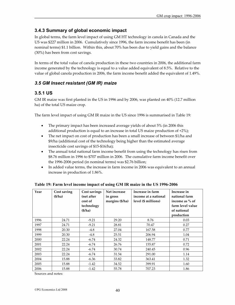
GM crop impact: 1996-2006
©PG Economics Ltd 2008 40
3.4.3 Summary of global economic impact In global terms, the farm level impact of using GM HT technology in canola in Canada and the US was $227 million in 2006. Cumulatively since 1996, the farm income benefit has been (in nominal terms) $1.1 billion. Within this, about 70% has been due to yield gains and the balance (30%) has been from cost savings. In terms of the total value of canola production in these two countries in 2006, the additional farm income generated by the technology is equal to a value added equivalent of 8.5%. Relative to the value of global canola production in 2006, the farm income benefit added the equivalent of 1.49%.
3.5 GM Insect resistant (GM IR) maize
3.5.1 US GM IR maize was first planted in the US in 1996 and by 2006, was planted on 40% (12.7 million ha) of the total US maize crop. The farm level impact of using GM IR maize in the US since 1996 is summarised in Table 19:
• The primary impact has been increased average yields of about 5% (in 2006 this additional production is equal to an increase in total US maize production of +2%);
• The net impact on cost of production has been a small increase of between $1/ha and $9/ha (additional cost of the technology being higher than the estimated average insecticide cost savings of $15-$16/ha);
• The annual total national farm income benefit from using the technology has risen from $8.76 million in 1996 to $707 million in 2006. The cumulative farm income benefit over the 1996-2006 period (in nominal terms) was $2.76 billion;
• In added value terms, the increase in farm income in 2006 was equivalent to an annual increase in production of 1.86%.
Table 19: Farm level income impact of using GM IR maize in the US 1996-2006
Year Cost saving ($/ha)
Cost savings (net after cost of technology ($/ha)
Net increase in gross margins ($/ha)
Increase in farm income at a national level ($ millions)
Increase in national farm income as % of farm level value of national production
1996 24.71 -9.21 29.20 8.76 0.03 1997 24.71 -9.21 28.81 70.47 0.27 1998 20.30 -4.8 27.04 167.58 0.77 1999 20.30 -4.8 25.51 206.94 1.04 2000 22.24 -6.74 24.32 148.77 0.71 2001 22.24 -6.74 26.76 155.87 0.72 2002 22.24 -6.74 30.74 240.45 0.96 2003 22.24 -6.74 31.54 291.00 1.14 2004 15.88 -6.36 33.82 363.41 1.32 2005 15.88 -1.42 34.52 399.91 1.60 2006 15.88 -1.42 55.78 707.23 1.86 Sources and notes:

GM crop impact: 1996-2006
©PG Economics Ltd 2008 41
1. Impact data based on a combination of studies including the ISAAA (James) review (2002), Marra et al and NCFAP 2001, 2003 and 2006
2. Yield impact +5% based on average of findings of above studies 3. Insecticide cost savings based on NCFAP 2003 and 2005 4. –ve value for net cost savings means the cost of the technology is greater than the other cost savings
3.5.2 Canada GM IR maize has also been grown commercially in Canada since 1996. In 2006 it accounted for 49% of the total Canadian maize crop of 1.33 million ha. The impact of GM IR maize in Canada has been very similar to the impact in the US (similar yield and cost of production impacts). At the national level, in 2006 the additional farm income generated from the use of GM IR maize was $31.6 million and cumulatively since 1996 the additional farm income (in nominal terms) was $143.6 million (Figure 12).
Figure 12: National farm income impact of using GM IR maize in Canada 1996-2006
Notes: 1. Yield increase of 5% based on industry assessments (consistent with US analysis). Cost of technology and insecticide cost savings based on US analysis, 2. Bt area planted in 1996 = 1,000 ha, 3. All values for prices and costs denominated in Canadian dollars have been converted to US dollars at the annual average exchange rate in each year
3.5.3 Argentina In 2006, GM IR maize traits were planted on 73% of the total Argentine maize crop (GM IR varieties were first planted in 1998). The main impact of using the technology on farm profitability has been via yield increases. Various studies (eg, see ISAAA review in James (2002)) have identified an average yield increase in the region of 8% to 10%, hence an average of 9% has been used in the analysis up to 2004. More recent trade source estimates provided to the authors put the average yield increased in the last 2-3 years to be between 5% and 6%. Accordingly our analysis uses a yield increase value of 5.5% for the years from 2004.

GM crop impact: 1996-2006
©PG Economics Ltd 2008 42
No savings in costs of production have arisen for most farmers because very few maize growers in Argentina have traditionally used insecticides as a method of control for corn boring pests. As such, average costs of production have increased by $20/ha-$22/ha (the cost of the technology). The net impact on farm profit margins (inclusive of the yield gain) has been an increase of about $20/ha, although in 2006 with higher world maize prices this has increased to about $30/ha. In 2006 the national level impact on profitability was an increase of $59 million (an added value equal to 2.2% of the total value of production). Cumulatively, the farm income gain since 1997 has been $193 million.
3.5.4 South Africa GM IR maize has been grown commercially in South Africa since 2000. In 2006, 34% of the country’s total maize crop of 2.9 million ha used GM IR cultivars. The impact on farm profitability is summarised in Table 20. The main impact has been an average yield improvement of between 5% and 32% in the years 2000-2004, with an average of about 15% (used as the basis for analysis in 2005 and 2006). The cost of the technology $8-$17/ha has broadly been equal to the average cost savings from no longer applying insecticides to control corn borer pests. At the national level, the increase in farm income in 2006 was $64 million and cumulatively since 2000 it has been $132 million. In terms of national maize production, the use of Bt technology on 34% of the planted area has resulted in a net increase in national maize production of 5.1% in 2006. The value of the additional income generated was also equivalent to an annual increase in production of about 4.3%.
Table 20: Farm level income impact of using GM IR maize in South Africa 2000-2006
Year Cost savings ($/ha) Net cost savings inclusive of cost of technology ($/ha)
Net increase in gross margin ($/ha)
Impact on farm income at a national level ($ millions)
2000 13.98 1.87 43.77 3.31 2001 11.27 1.51 34.60 4.46 2002 8.37 0.6 113.98 19.35 2003 12.82 0.4 63.72 14.66 2004 14.73 0.46 20.76 8.43 2005 15.25 0.47 48.66 19.03 2006 14.32 -2.36 63.75 63.05 Sources and notes:
1. Impact data (sources: Gouse (2005 & 2006)) 2. Negative value for the net cost savings = a net increase in costs (ie, the extra cost of the technology
was greater than the other (eg, less expenditure on insecticides) cost savings 3. All values for prices and costs denominated in South African Rand have been converted to US
dollars at the annual average exchange rate in each year
3.5.5 Spain Spain has been commercially growing GM IR maize since 1998 and in 2006, 15% (54,000 ha) of the country’s maize crop was planted to varieties containing a GM IR trait.
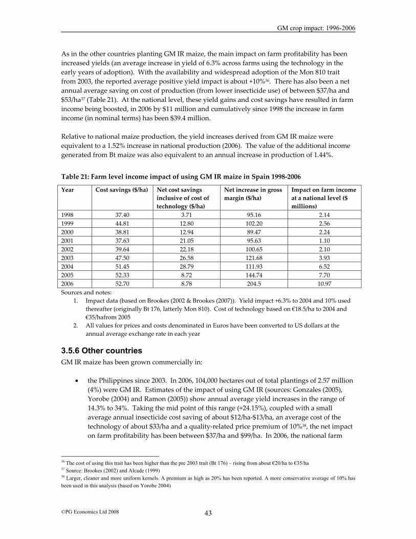
GM crop impact: 1996-2006
©PG Economics Ltd 2008 43
As in the other countries planting GM IR maize, the main impact on farm profitability has been increased yields (an average increase in yield of 6.3% across farms using the technology in the early years of adoption). With the availability and widespread adoption of the Mon 810 trait from 2003, the reported average positive yield impact is about +10%36. There has also been a net annual average saving on cost of production (from lower insecticide use) of between $37/ha and $53/ha37 (Table 21). At the national level, these yield gains and cost savings have resulted in farm income being boosted, in 2006 by $11 million and cumulatively since 1998 the increase in farm income (in nominal terms) has been $39.4 million. Relative to national maize production, the yield increases derived from GM IR maize were equivalent to a 1.52% increase in national production (2006). The value of the additional income generated from Bt maize was also equivalent to an annual increase in production of 1.44%.
Table 21: Farm level income impact of using GM IR maize in Spain 1998-2006
Year Cost savings ($/ha) Net cost savings inclusive of cost of technology ($/ha)
Net increase in gross margin ($/ha)
Impact on farm income at a national level ($ millions)
1998 37.40 3.71 95.16 2.14 1999 44.81 12.80 102.20 2.56 2000 38.81 12.94 89.47 2.24 2001 37.63 21.05 95.63 1.10 2002 39.64 22.18 100.65 2.10 2003 47.50 26.58 121.68 3.93 2004 51.45 28.79 111.93 6.52 2005 52.33 8.72 144.74 7.70 2006 52.70 8.78 204.5 10.97 Sources and notes:
1. Impact data (based on Brookes (2002 & Brookes (2007)). Yield impact +6.3% to 2004 and 10% used thereafter (originally Bt 176, latterly Mon 810). Cost of technology based on €18.5/ha to 2004 and €35/hafrom 2005
2. All values for prices and costs denominated in Euros have been converted to US dollars at the annual average exchange rate in each year
3.5.6 Other countries GM IR maize has been grown commercially in:
• the Philippines since 2003. In 2006, 104,000 hectares out of total plantings of 2.57 million (4%) were GM IR. Estimates of the impact of using GM IR (sources: Gonzales (2005), Yorobe (2004) and Ramon (2005)) show annual average yield increases in the range of 14.3% to 34%. Taking the mid point of this range (+24.15%), coupled with a small average annual insecticide cost saving of about $12/ha-$13/ha, an average cost of the technology of about $33/ha and a quality-related price premium of 10%38, the net impact on farm profitability has been between $37/ha and $99/ha. In 2006, the national farm
36 The cost of using this trait has been higher than the pre 2003 trait (Bt 176) – rising from about €20/ha to €35/ha 37 Source: Brookes (2002) and Alcade (1999) 38 Larger, cleaner and more uniform kernels. A premium as high as 20% has been reported. A more conservative average of 10% has been used in this analysis (based on Yorobe 2004)
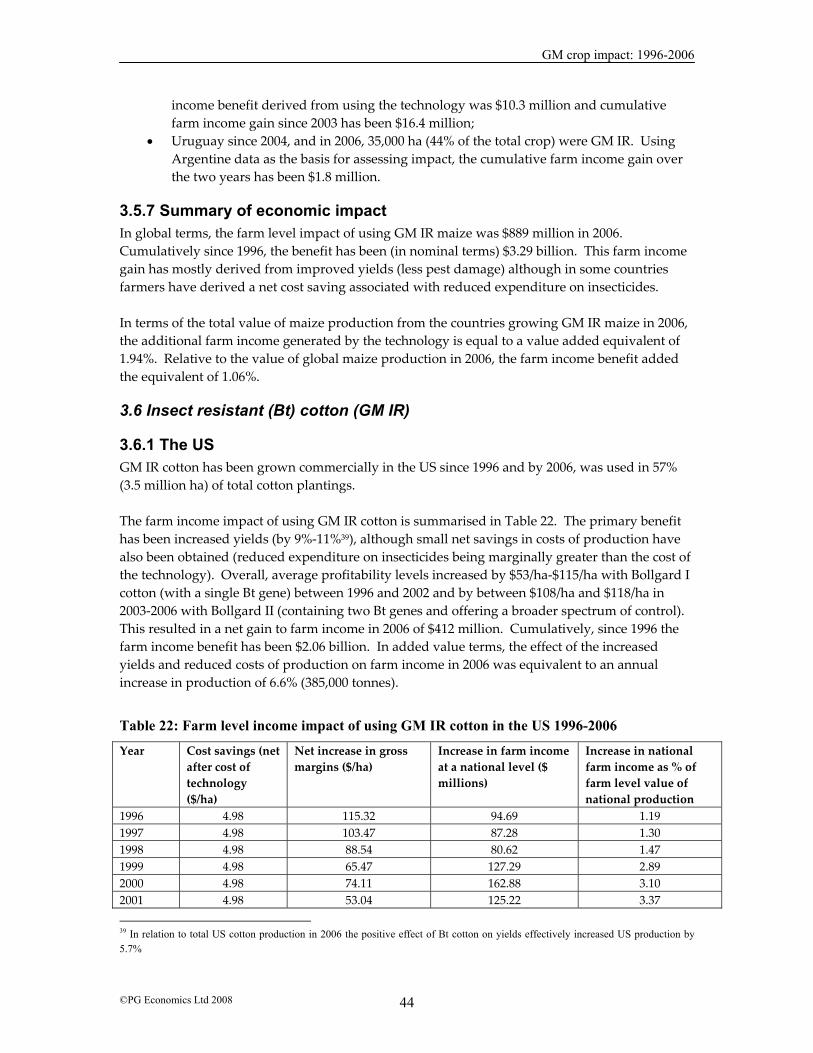
GM crop impact: 1996-2006
©PG Economics Ltd 2008 44
income benefit derived from using the technology was $10.3 million and cumulative farm income gain since 2003 has been $16.4 million;
• Uruguay since 2004, and in 2006, 35,000 ha (44% of the total crop) were GM IR. Using Argentine data as the basis for assessing impact, the cumulative farm income gain over the two years has been $1.8 million.
3.5.7 Summary of economic impact In global terms, the farm level impact of using GM IR maize was $889 million in 2006. Cumulatively since 1996, the benefit has been (in nominal terms) $3.29 billion. This farm income gain has mostly derived from improved yields (less pest damage) although in some countries farmers have derived a net cost saving associated with reduced expenditure on insecticides. In terms of the total value of maize production from the countries growing GM IR maize in 2006, the additional farm income generated by the technology is equal to a value added equivalent of 1.94%. Relative to the value of global maize production in 2006, the farm income benefit added the equivalent of 1.06%.
3.6 Insect resistant (Bt) cotton (GM IR)
3.6.1 The US GM IR cotton has been grown commercially in the US since 1996 and by 2006, was used in 57% (3.5 million ha) of total cotton plantings. The farm income impact of using GM IR cotton is summarised in Table 22. The primary benefit has been increased yields (by 9%-11%39), although small net savings in costs of production have also been obtained (reduced expenditure on insecticides being marginally greater than the cost of the technology). Overall, average profitability levels increased by $53/ha-$115/ha with Bollgard I cotton (with a single Bt gene) between 1996 and 2002 and by between $108/ha and $118/ha in 2003-2006 with Bollgard II (containing two Bt genes and offering a broader spectrum of control). This resulted in a net gain to farm income in 2006 of $412 million. Cumulatively, since 1996 the farm income benefit has been $2.06 billion. In added value terms, the effect of the increased yields and reduced costs of production on farm income in 2006 was equivalent to an annual increase in production of 6.6% (385,000 tonnes).
Table 22: Farm level income impact of using GM IR cotton in the US 1996-2006
Year Cost savings (net after cost of technology ($/ha)
Net increase in gross margins ($/ha)
Increase in farm income at a national level ($ millions)
Increase in national farm income as % of farm level value of national production
1996 4.98 115.32 94.69 1.19 1997 4.98 103.47 87.28 1.30 1998 4.98 88.54 80.62 1.47 1999 4.98 65.47 127.29 2.89 2000 4.98 74.11 162.88 3.10 2001 4.98 53.04 125.22 3.37
39 In relation to total US cotton production in 2006 the positive effect of Bt cotton on yields effectively increased US production by 5.7%

GM crop impact: 1996-2006
©PG Economics Ltd 2008 45
2002 4.98 69.47 141.86 3.11 2003 5.78 120.49 239.98 4.27 2004 5.78 107.47 261.23 4.82 2005 24.48 117.81 332.41 5.97 2006 24.48 116.87 411.76 6.56 Sources and notes:
1. Impact data based on NCFAP 2001, 2003 and 2006, Marra M (2002) and Mullins & Hudson (2004) 2. Yield impact +9% 1996-2002 Bollgard I and +11% 2003-2006 Bollgard II 3. Cost of technology: 1996-2002 Bollgard I $58.27/ha, 2003-2004 Bollgard II $68.32/ha, $49.62/ha 2005
& 2006 4. Insecticide cost savings $63.26/ha 1996-2002, $74.10/ha 2003-2006
3.6.2 China China first planted GM IR cotton in 1997, since when the area planted to GM IR varieties has increased to 65% of the total 5.6 million ha crop in 2006. As in the US, a major farm income impact has been via higher yields of 8% to 10% on the crops using the technology, although there have also been significant cost savings on insecticides used and the labour previously used to undertake spraying. Overall, annual average costs have fallen by about $145/ha-$192/ha and annual average profitability improved by $226/ha-$327/ha. In 2006, the net national gain to farm income was $0.82 billion ( Table 23). Cumulatively since 1997 the farm income benefit has been $5.82 billion. In added value terms, the effect of the increased yields and reduced costs of production on farm income in 2006 was equivalent to an annual increase in production of nearly 16.4% (1.2 million tonnes).
Table 23: Farm level income impact of using GM IR cotton in China 1997-2006
Year Cost savings (net after cost of technology ($/ha)
Net increase in gross margins ($/ha)
Increase in farm income at a national level ($ millions)
Increase in national farm income as % of farm level value of national production
1997 194 333 11.33 0.13 1998 194 310 80.97 1.15 1999 200 278 181.67 4.62 2000 -14 123 150.18 2.61 2001 378 472 1,026.26 20.55 2002 194 327 687.27 11.19 2003 194 328 917.00 12.15 2004 194 299 1,105.26 16.89 2005 145 256 845.58 13.57 2006 146 226 816.66 16.45 Sources and notes:
1. Impact data based on Prey et al (2002) which covered the years 1999-2001. Other years based on average of the 3 years, except 2005 & 2006 based on Shachuan (2006) – personal comunication
2. Negative cost savings in 2000 reflect a year of high pest pressure (of pests not the target of GM IR technology) which resulted in above average use of insecticides on GM IR using farms
3. Yield impact +8% 1997-1999 and +10% 2000 onwards 4. Negative value for the net cost savings in 2000 = a net increase in costs (ie, the extra cost of the
technology was greater than the savings on insecticide expenditure – a year of lower than average bollworm problems
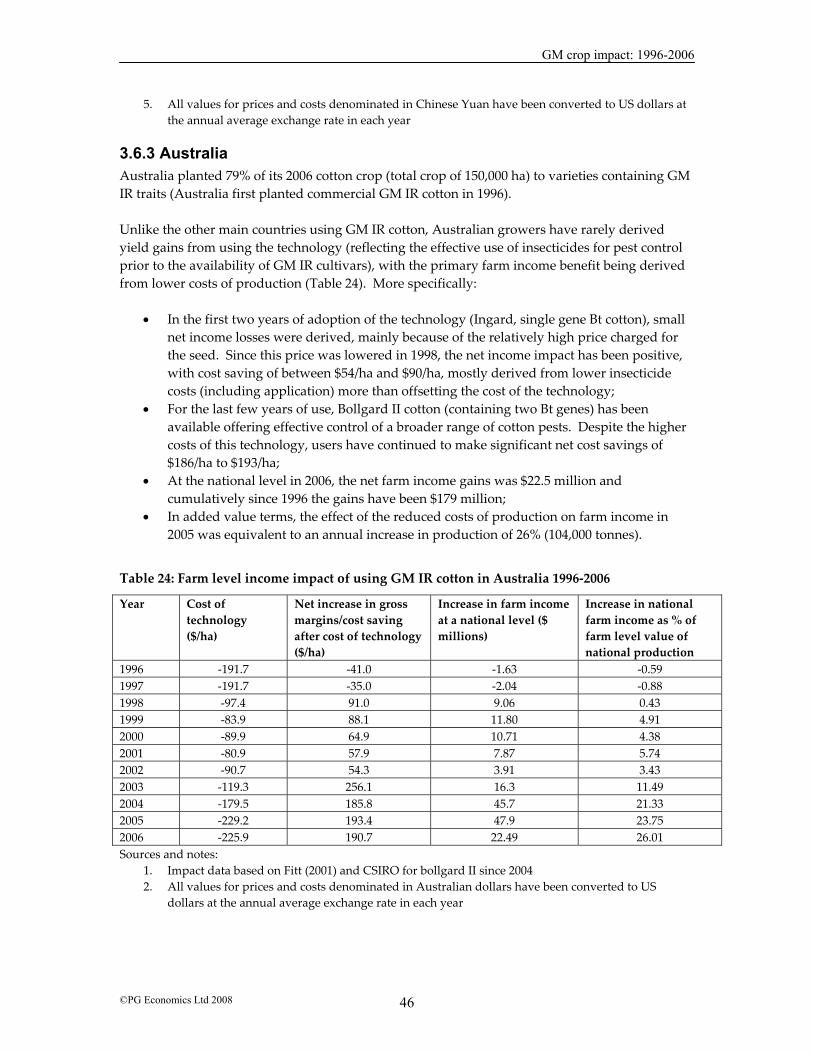
GM crop impact: 1996-2006
©PG Economics Ltd 2008 46
5. All values for prices and costs denominated in Chinese Yuan have been converted to US dollars at the annual average exchange rate in each year
3.6.3 Australia Australia planted 79% of its 2006 cotton crop (total crop of 150,000 ha) to varieties containing GM IR traits (Australia first planted commercial GM IR cotton in 1996). Unlike the other main countries using GM IR cotton, Australian growers have rarely derived yield gains from using the technology (reflecting the effective use of insecticides for pest control prior to the availability of GM IR cultivars), with the primary farm income benefit being derived from lower costs of production (Table 24). More specifically:
• In the first two years of adoption of the technology (Ingard, single gene Bt cotton), small net income losses were derived, mainly because of the relatively high price charged for the seed. Since this price was lowered in 1998, the net income impact has been positive, with cost saving of between $54/ha and $90/ha, mostly derived from lower insecticide costs (including application) more than offsetting the cost of the technology;
• For the last few years of use, Bollgard II cotton (containing two Bt genes) has been available offering effective control of a broader range of cotton pests. Despite the higher costs of this technology, users have continued to make significant net cost savings of $186/ha to $193/ha;
• At the national level in 2006, the net farm income gains was $22.5 million and cumulatively since 1996 the gains have been $179 million;
• In added value terms, the effect of the reduced costs of production on farm income in 2005 was equivalent to an annual increase in production of 26% (104,000 tonnes).
Table 24: Farm level income impact of using GM IR cotton in Australia 1996-2006
Year Cost of technology ($/ha)
Net increase in gross margins/cost saving after cost of technology ($/ha)
Increase in farm income at a national level ($ millions)
Increase in national farm income as % of farm level value of national production
1996 -191.7 -41.0 -1.63 -0.59 1997 -191.7 -35.0 -2.04 -0.88 1998 -97.4 91.0 9.06 0.43 1999 -83.9 88.1 11.80 4.91 2000 -89.9 64.9 10.71 4.38 2001 -80.9 57.9 7.87 5.74 2002 -90.7 54.3 3.91 3.43 2003 -119.3 256.1 16.3 11.49 2004 -179.5 185.8 45.7 21.33 2005 -229.2 193.4 47.9 23.75 2006 -225.9 190.7 22.49 26.01 Sources and notes:
1. Impact data based on Fitt (2001) and CSIRO for bollgard II since 2004 2. All values for prices and costs denominated in Australian dollars have been converted to US
dollars at the annual average exchange rate in each year
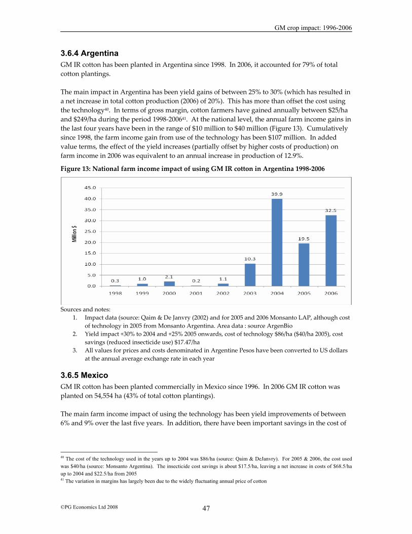
GM crop impact: 1996-2006
©PG Economics Ltd 2008 47
3.6.4 Argentina GM IR cotton has been planted in Argentina since 1998. In 2006, it accounted for 79% of total cotton plantings. The main impact in Argentina has been yield gains of between 25% to 30% (which has resulted in a net increase in total cotton production (2006) of 20%). This has more than offset the cost using the technology40. In terms of gross margin, cotton farmers have gained annually between $25/ha and $249/ha during the period 1998-200641. At the national level, the annual farm income gains in the last four years have been in the range of $10 million to $40 million (Figure 13). Cumulatively since 1998, the farm income gain from use of the technology has been $107 million. In added value terms, the effect of the yield increases (partially offset by higher costs of production) on farm income in 2006 was equivalent to an annual increase in production of 12.9%.
Figure 13: National farm income impact of using GM IR cotton in Argentina 1998-2006
Sources and notes: 1. Impact data (source: Qaim & De Janvry (2002) and for 2005 and 2006 Monsanto LAP, although cost
of technology in 2005 from Monsanto Argentina. Area data : source ArgenBio 2. Yield impact +30% to 2004 and +25% 2005 onwards, cost of technology $86/ha ($40/ha 2005), cost
savings (reduced insecticide use) $17.47/ha 3. All values for prices and costs denominated in Argentine Pesos have been converted to US dollars
at the annual average exchange rate in each year
3.6.5 Mexico GM IR cotton has been planted commercially in Mexico since 1996. In 2006 GM IR cotton was planted on 54,554 ha (43% of total cotton plantings). The main farm income impact of using the technology has been yield improvements of between 6% and 9% over the last five years. In addition, there have been important savings in the cost of
40 The cost of the technology used in the years up to 2004 was $86/ha (source: Qaim & DeJanvry). For 2005 & 2006, the cost used was $40/ha (source: Monsanto Argentina). The insecticide cost savings is about $17.5/ha, leaving a net increase in costs of $68.5/ha up to 2004 and $22.5/ha from 2005 41 The variation in margins has largely been due to the widely fluctuating annual price of cotton
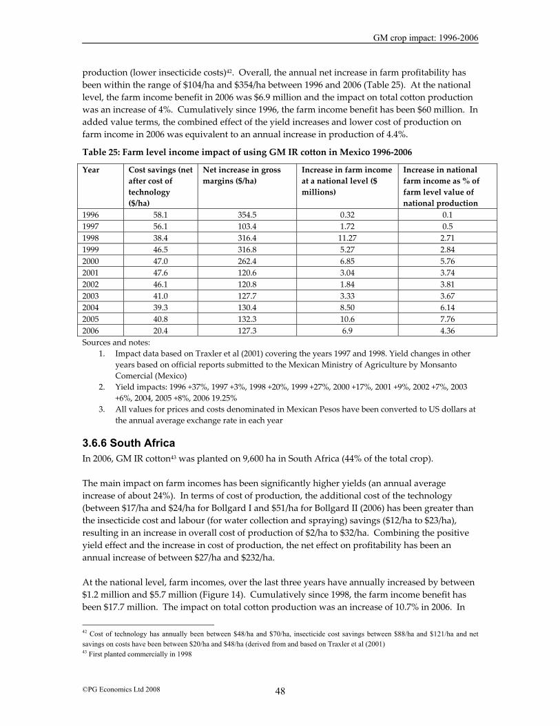
GM crop impact: 1996-2006
©PG Economics Ltd 2008 48
production (lower insecticide costs)42. Overall, the annual net increase in farm profitability has been within the range of $104/ha and $354/ha between 1996 and 2006 (Table 25). At the national level, the farm income benefit in 2006 was $6.9 million and the impact on total cotton production was an increase of 4%. Cumulatively since 1996, the farm income benefit has been $60 million. In added value terms, the combined effect of the yield increases and lower cost of production on farm income in 2006 was equivalent to an annual increase in production of 4.4%.
Table 25: Farm level income impact of using GM IR cotton in Mexico 1996-2006
Year Cost savings (net after cost of technology ($/ha)
Net increase in gross margins ($/ha)
Increase in farm income at a national level ($ millions)
Increase in national farm income as % of farm level value of national production
1996 58.1 354.5 0.32 0.1 1997 56.1 103.4 1.72 0.5 1998 38.4 316.4 11.27 2.71 1999 46.5 316.8 5.27 2.84 2000 47.0 262.4 6.85 5.76 2001 47.6 120.6 3.04 3.74 2002 46.1 120.8 1.84 3.81 2003 41.0 127.7 3.33 3.67 2004 39.3 130.4 8.50 6.14 2005 40.8 132.3 10.6 7.76 2006 20.4 127.3 6.9 4.36 Sources and notes:
1. Impact data based on Traxler et al (2001) covering the years 1997 and 1998. Yield changes in other years based on official reports submitted to the Mexican Ministry of Agriculture by Monsanto Comercial (Mexico)
2. Yield impacts: 1996 +37%, 1997 +3%, 1998 +20%, 1999 +27%, 2000 +17%, 2001 +9%, 2002 +7%, 2003 +6%, 2004, 2005 +8%, 2006 19.25%
3. All values for prices and costs denominated in Mexican Pesos have been converted to US dollars at the annual average exchange rate in each year
3.6.6 South Africa In 2006, GM IR cotton43 was planted on 9,600 ha in South Africa (44% of the total crop). The main impact on farm incomes has been significantly higher yields (an annual average increase of about 24%). In terms of cost of production, the additional cost of the technology (between $17/ha and $24/ha for Bollgard I and $51/ha for Bollgard II (2006) has been greater than the insecticide cost and labour (for water collection and spraying) savings ($12/ha to $23/ha), resulting in an increase in overall cost of production of $2/ha to $32/ha. Combining the positive yield effect and the increase in cost of production, the net effect on profitability has been an annual increase of between $27/ha and $232/ha. At the national level, farm incomes, over the last three years have annually increased by between $1.2 million and $5.7 million (Figure 14). Cumulatively since 1998, the farm income benefit has been $17.7 million. The impact on total cotton production was an increase of 10.7% in 2006. In
42 Cost of technology has annually been between $48/ha and $70/ha, insecticide cost savings between $88/ha and $121/ha and net savings on costs have been between $20/ha and $48/ha (derived from and based on Traxler et al (2001) 43 First planted commercially in 1998
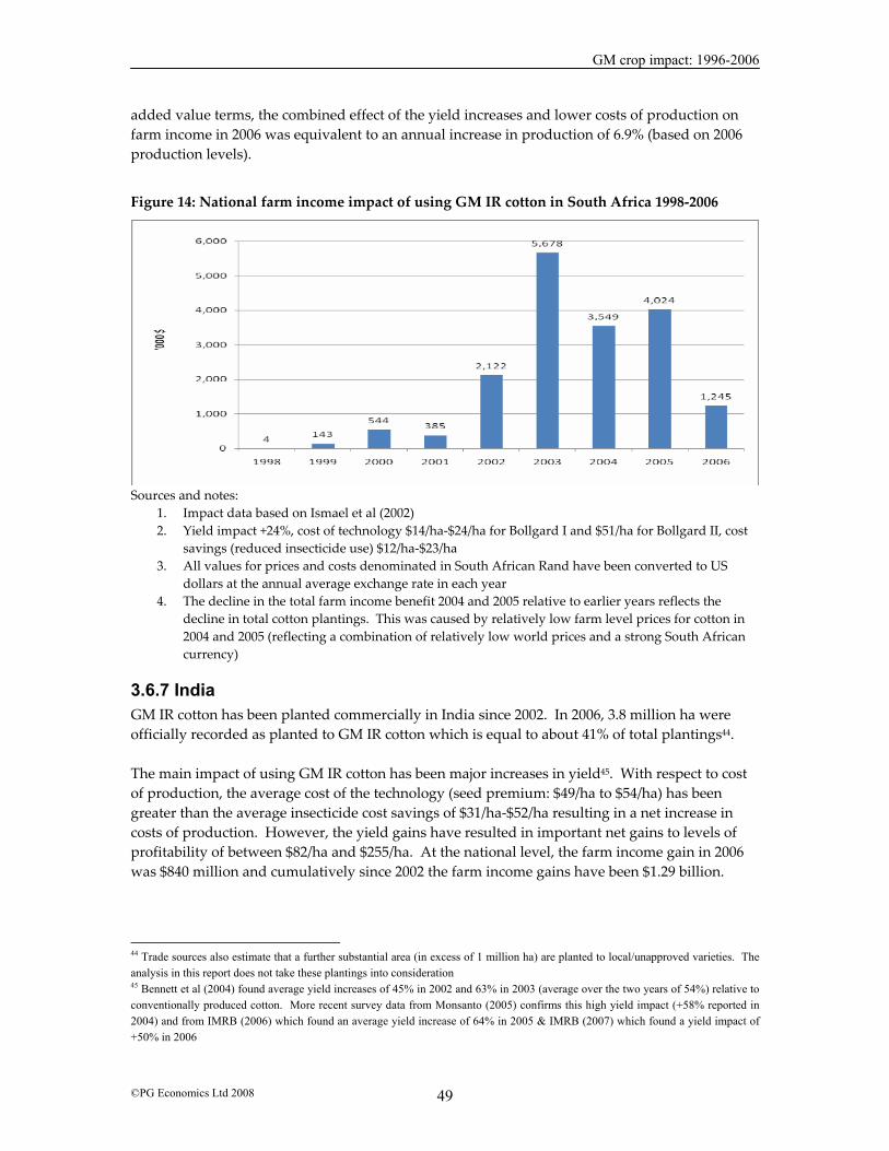
GM crop impact: 1996-2006
©PG Economics Ltd 2008 49
added value terms, the combined effect of the yield increases and lower costs of production on farm income in 2006 was equivalent to an annual increase in production of 6.9% (based on 2006 production levels).
Figure 14: National farm income impact of using GM IR cotton in South Africa 1998-2006
Sources and notes: 1. Impact data based on Ismael et al (2002) 2. Yield impact +24%, cost of technology $14/ha-$24/ha for Bollgard I and $51/ha for Bollgard II, cost
savings (reduced insecticide use) $12/ha-$23/ha 3. All values for prices and costs denominated in South African Rand have been converted to US
dollars at the annual average exchange rate in each year 4. The decline in the total farm income benefit 2004 and 2005 relative to earlier years reflects the
decline in total cotton plantings. This was caused by relatively low farm level prices for cotton in 2004 and 2005 (reflecting a combination of relatively low world prices and a strong South African currency)
3.6.7 India GM IR cotton has been planted commercially in India since 2002. In 2006, 3.8 million ha were officially recorded as planted to GM IR cotton which is equal to about 41% of total plantings44. The main impact of using GM IR cotton has been major increases in yield45. With respect to cost of production, the average cost of the technology (seed premium: $49/ha to $54/ha) has been greater than the average insecticide cost savings of $31/ha-$52/ha resulting in a net increase in costs of production. However, the yield gains have resulted in important net gains to levels of profitability of between $82/ha and $255/ha. At the national level, the farm income gain in 2006 was $840 million and cumulatively since 2002 the farm income gains have been $1.29 billion.
44 Trade sources also estimate that a further substantial area (in excess of 1 million ha) are planted to local/unapproved varieties. The analysis in this report does not take these plantings into consideration 45 Bennett et al (2004) found average yield increases of 45% in 2002 and 63% in 2003 (average over the two years of 54%) relative to conventionally produced cotton. More recent survey data from Monsanto (2005) confirms this high yield impact (+58% reported in 2004) and from IMRB (2006) which found an average yield increase of 64% in 2005 & IMRB (2007) which found a yield impact of +50% in 2006

GM crop impact: 1996-2006
©PG Economics Ltd 2008 50
Table 26: Farm level income impact of using GM IR cotton in India 2002-2006
Year Cost savings (net after cost of technology ($/ha)
Net increase in gross margins ($/ha)
Increase in farm income at a national level ($ millions)
Increase in national farm income as % of farm level value of national production
2002 -12.42 82.66 3.69 0.26 2003 -16.2 209.85 20.98 2.83 2004 -13.56 193.36 96.68 3.07 2005 -22.25 255.96 332.74 9.38 2006 3.52 221.02 839.89 20.72 Sources and notes:
1. Impact data based on Bennett et al (2004) and IMRB (2005 & 2006) 2. All values for prices and costs denominated in Indian Rupees have been converted to US dollars at
the annual average exchange rate in each year The impact on total cotton production was an increase of 21% in 2006 and in added value terms, the combined effect of the yield increases and higher costs of production on farm income in 2006 was equivalent to an annual increase in production of 14% (based on the 2006 production level that is inclusive of the GM IR related yield gains).
3.6.8 Brazil GM IR cotton was planted commercially in Brazil for the first time in 2006 (on 134,000 ha). On the basis of industry estimates of impact; an average yield gains were +6% and the net cost saving (reduced expenditure on insecticides after deduction of the premium paid for using the technology) was about +$24/ha. In total the farm income gain in 2006 was $127/ha and at a national level this amounts to +$17 million.
3.6.9 Other countries GM IR cotton has been grown commercially in Columbia since 2002 (13,380 ha planted in 2006 out of a total cotton crop of 72,000 ha). We are not aware of any impact analysis of these crops having yet been undertaken. Drawing on the analysis of impact in Mexico and applying this to Columbia (a 6.7% yield increase and a net reduction in costs of production of $20/ha to $40/ha), this would put the national gain to farm income in 2006 at $0.9 million and the cumulative farm income gain since 2002 has been $5.2 million.
3.6.9 Summary of global impact In global terms, the farm level impact of using GM IR cotton was $2.15 billion in 2006. Cumulatively since 1996, the farm income benefit has been (in nominal terms) $9.57 billion. Within this, 58% of the farm income gain has derived from yield gains (less pest damage) and the balance (42%) from reduced expenditure on crop protection (spraying of insecticides). In terms of the total value of cotton production from the countries growing GM IR in 2006, the additional farm income generated by the technology is equal to a value added equivalent of 13.1% (based on the 2006 production level inclusive of the GM IR related yield gains). Relative to the value of global cotton production in 2006, the farm income benefit added the equivalent of 7.85%.
GM crop impact: 1996-2006
©PG Economics Ltd 2008 51
3.7 Other GM crops
3.7.1 Maize/corn rootworm resistance GM rootworm resistant (CRW) corn has been planted commercially in the US for four years. In 2006, there were 4 million ha of CRW corn (12.8% of the total US crop). The main farm income impact46 has been higher yields of about 5% relative to conventionally treated corn. The impact on average costs of production has been +$2/ha to -$10/ha (based on an average cost of the technology of $35/ha-$42/ha and an insecticide cost saving of $32/ha-$37/ha). As a result, the net impact on farm profitability has been +$28/ha to +$60/ha. At the national level, farm incomes increased by $4.6 million in 2003, rising to $241 million in 2006. Cumulatively since 2003, the total farm income gain from the use of CRW technology in the US corn crop has been $335 million. CRW cultivars were also planted commercially for the first time in 2004 in Canada. In 2006 the area planted to CRW resistant varieties was 17,400 ha. Based on US costs, insecticide cost savings and yield impacts, this has resulted in additional income at the national level of $933,000 in 2006 (cumulative total since 2004 of $1.5 million). At the global level, the extra farm income derived from GM CRW maize use since 2003 has been $337 million. In 2006, the additional farm income generated from use of the technology was equal to 0.29% of the value of the global maize crop.
3.7.2 Virus resistant papaya Ringspot resistant papaya has been commercially grown in the US (State of Hawaii) since 1999, and in 2006 about 55% of the state’s papaya crop was GM virus resistant (480 ha). The main farm income impact of this GM crop has been to significantly increase yields relative to conventional varieties. Compared to the average yield in the last year before the first GM cultivation (1998), the annual average yield increase of GM papaya relative to conventional crops has been within a range of +16% to +77% (18% in 2005 and 2006 with an average of about +40%). At a state level this is equivalent to a 10% increase in total papaya production in 2006. In terms of profitability47, the net annual impact has been an improvement of between $3,032/ha and $11,412/ha, and in 2006 this amounted to a total state level benefit of $1.6 million. Cumulatively, the farm income benefit since 1999 has been $23.1 million.
3.7.3 Virus resistant squash GM virus resistant squash has also been grown in some states of the US since 2003 and is estimated to have been planted on about 2,840 ha in 200648 (about 10% of the total crop in the US). Based on analysis from NCFAP (2005), the primary farm income impact of using GM virus resistant squash has been derived from higher yields, which in 2006 added a net gain to users of $25 million. Cumulatively, the farm income benefit since 2003 has been $70 million. 46 Impact data based on NCFAP (2003 and 2005) and Rice (2004) 47 Impact data based on NCFAP 2003 and 2005 48 Mostly found in Georgia and Florida
GM crop impact: 1996-2006
©PG Economics Ltd 2008 52
3.7.4 Insect resistant potatoes GM insect resistant potatoes were also grown commercially in the US between 1996 and 2000 (planted on 4% of the total US potato crop in 1999 (30,000 ha). This technology was withdrawn in 2001 when the technology provider (Monsanto) withdrew from the market to concentrate on GM trait development in maize, soybeans, cotton and canola. This commercial decision was also probably influenced by the decision of some leading potato processors and fast food outlets to stop using GM potatoes because of perceived concerns about this issue from some of their consumers, even though the GM potato provided the producer and processor with a lower cost, higher yielding and more consistent product. It also delivered significant reductions in insecticide use (NCFAP 2001).
3.8 Other farm level economic impacts of using GM crops As well as the tangible and quantifiable impacts on farm profitability presented in the sub-sections above, there are other important, more intangible (difficult to quantify) impacts of an economic nature. Many of the studies49 of the impact of GM crops have identified the following reasons as being important influences for adoption of the technology: Herbicide tolerant crops
• increased management flexibility that comes from a combination of the ease of use associated with broad-spectrum, post emergent herbicides like glyphosate and the increased/longer time window for spraying;
• In a conventional crop, post-emergent weed control relies on herbicide applications before the weeds and crop are well established. As a result, the crop may suffer ‘knock-back’ to its growth from the effects of the herbicide. In the GM HT crop, this problem is avoided because the crop is both tolerant to the herbicide and spraying can occur at a later stage when the crop is better able to withstand any possible “knock-back” effects;
• Facilitates the adoption of conservation or no tillage systems. This provides for additional cost savings such as reduced labour and fuel costs associated with ploughing, additional moisture retention and reductions in levels of soil erosion;
• Improved weed control has contributed to reduced harvesting costs – cleaner crops have resulted in reduced times for harvesting. It has also improved harvest quality and led to higher levels of quality price bonuses in some regions (eg, Romania);
• Elimination of potential damage caused by soil-incorporated residual herbicides in follow-on crops.
Insect resistant crops
• Production risk management/insurance purposes – it takes away the worry of significant pest damage occurring;
• A ‘convenience’ benefit derived from having to devote less time to crop walking and/or applying insecticides;
• savings in energy use – mainly associated with less use of aerial spraying and less tillage; • savings in machinery use (for spraying and possibly reduced harvesting times);
49 For example, relating to HT soybeans; USDA 1999, Gianessi & Carpenter 2000, Qaim & Traxler 2002, Brookes 2005; relating to insect resistant maize , Rice 2004; relating to insect resistant cotton Ismael et al 2002, Pray et al 2002

GM crop impact: 1996-2006
©PG Economics Ltd 2008 53
• Higher quality of maize. There is a growing body of research evidence relating to the superior quality of Bt maize relative to conventional and organic maize from the perspective of having lower levels of mycotoxins. Evidence from Europe (as summarised in Brookes (2007) has shown a consistent pattern in which Bt maize exhibits significantly reduced levels of mycotoxins compared to conventional and organic alternatives. In terms of revenue from sales of corn, however, no reported premia for delivering product with lower levels of mycotoxin levels have, to date, been reported although where the adoption of the technology has resulted in reduced frequency of crops failing to meet maximum permissible fumonisin levels in grain maize (eg, in Spain), this delivers an important economic gain to farmers selling their grain to the food using sector;
• Improved health and safety for farmers and farm workers (from reduced handling and use of pesticides, especially in developing countries where many apply pesticides with little or no use of protective clothing and equipment);
• Shorter growing season (eg, for some cotton growers in India) which allows some farmers to plant a second crop in the same season50. Also some Indian cotton growers have reported knock on benefits for bee keepers as fewer bees are now lost to insecticide spraying.
As indicated above, quantifying these impacts is difficult. Some studies have attempted to quantify some of these benefits (eg, Qaim & Traxler (2002) quantified some of these in Argentina (a $3.65/hctare saving (-7.8%) in labour costs and a $6.82/ha (-28%) saving in machinery/fuel costs). Where identified, these cost savings have been included in the analysis presented in the preceding parts of section 3. Nevertheless, it is important to recognise that these largely intangible benefits are considered by many farmers as a primary reason for adoption of GM technology, and in some cases farmers have been willing to adopt for these reasons alone, even when the measurable impacts on yield and direct costs of production suggest marginal or no direct economic gain. As such, the estimates of the farm level benefits presented in the preceding sections probably understate the real vale of the technology to farmers.
3.9 GM technology adoption and size of farm This issue has been specifically examined in few pieces of research. Examples include:
• Fernandez-Cornejo & McBride (2000) examined the effect of size on adoption of GM crops in the US (using 1998 data). The a priori hypothesis used for the analysis was that the nature of the technology embodied in a variable input like seed (which is completely divisible and not a ‘lumpy’ input like machinery) should show that adoption of GM crops is not related to size. The analysis found that mean adoption rates appeared to increase with size of operation for herbicide tolerant crops (soybeans and maize) up to 50 hectares in size and then were fairly stable, whilst for Bt maize adoption appeared to increase with size. This analysis did, however not take into other factors affecting adoption such as education, awareness of new technology and willingness to adopt, income, access to credit and whether a farm was full or part time – all these are considered to affect adoption yet are also often correlated to size of farm. Overall, the study suggested that farm size has not been an important factor influencing adoption of GM crops;
50 Notably maize in India
GM crop impact: 1996-2006
©PG Economics Ltd 2008 54
• Brookes (2002) identified in Spain that the average size of farmer adopting Bt maize was 50 hectares and that many were much smaller than this (under 20 hectares). Size was not therefore considered to be an important factor affecting adoption, with many small farmers using the technology;
• Brookes (2005) also identified in Romania that the average size of farmer adopting HT soybeans was not related to size of farm;
• Pray et al (2002). This research into GM insect resistant cotton adoption in China illustrated that adoption has been by mostly small farmers (the average cotton grower in China plants between 0.3 and 0.5 ha of cotton);
• Adopters of insect resistant cotton and maize in South Africa have been drawn from both large and small farmers (see Morse et al 2004, Ismael et al 2002, Gouse (2006)).
Overall, the nature of findings from most studies where the nature and size of adopter has been a focus of research has shown that size of farm has not been a factor affecting use of GM technology. Both large and small farmers have adopted. Size of operation has not been a barrier to adoption and in 2006, 10.25 million farmers were using the technology globally, 90% of which were resource-poor farmers in developing countries.
3.10 Trade flows and related issues a) Share of global production As indicated in section 2, in 2006, GM plantings accounted for 33% of the global area planted to the crops of soybeans, maize, cotton and canola. At the crop level, the GM share of global plantings was 61.5%, 16.2%, 38.4% and 17.5% respectively for soybeans, maize, cotton and canola. In terms of additional production (derived from yield gains), in 2006, global production of soybeans, corn, cotton and canola were respectively +5%, +1.4%, +5.2% and +0.5% higher than levels would have otherwise been if GM technology had not been used by farmers (Table 27). This amounted to additional volumes of production of +11.6 million tonnes of soybeans, +9.65 million tonnes of corn, +1.38 million tonnes of cotton lint and +0.21 million tonnes of canola.
Table 27: Additional production of main crops in 2006 due to GM technology (million tonnes)
World production 2006 Additional production arising from GM
technology yield effect
% of world production arising from GM yield
effect Soybeans 235 11.6 5 Corn 703 9.65 1.4 Cotton (lint) 26.5 1.38 5.2 Canola 46.4 0.21 0.5 In area equivalent terms, if the GM technology used by farmers in 2006 had not been available, maintaining global production levels at the 2006 levels would have required additional plantings of 3.9 million ha of soybeans, 1 million ha of corn, 1.8 million ha of cotton and 0.15 million ha of canola.
b) Share of global exports Looking at the extent to which the leading GM producing countries are traders (exporters) of these crops and key derivatives (Table 28 and Table 29) show the following:
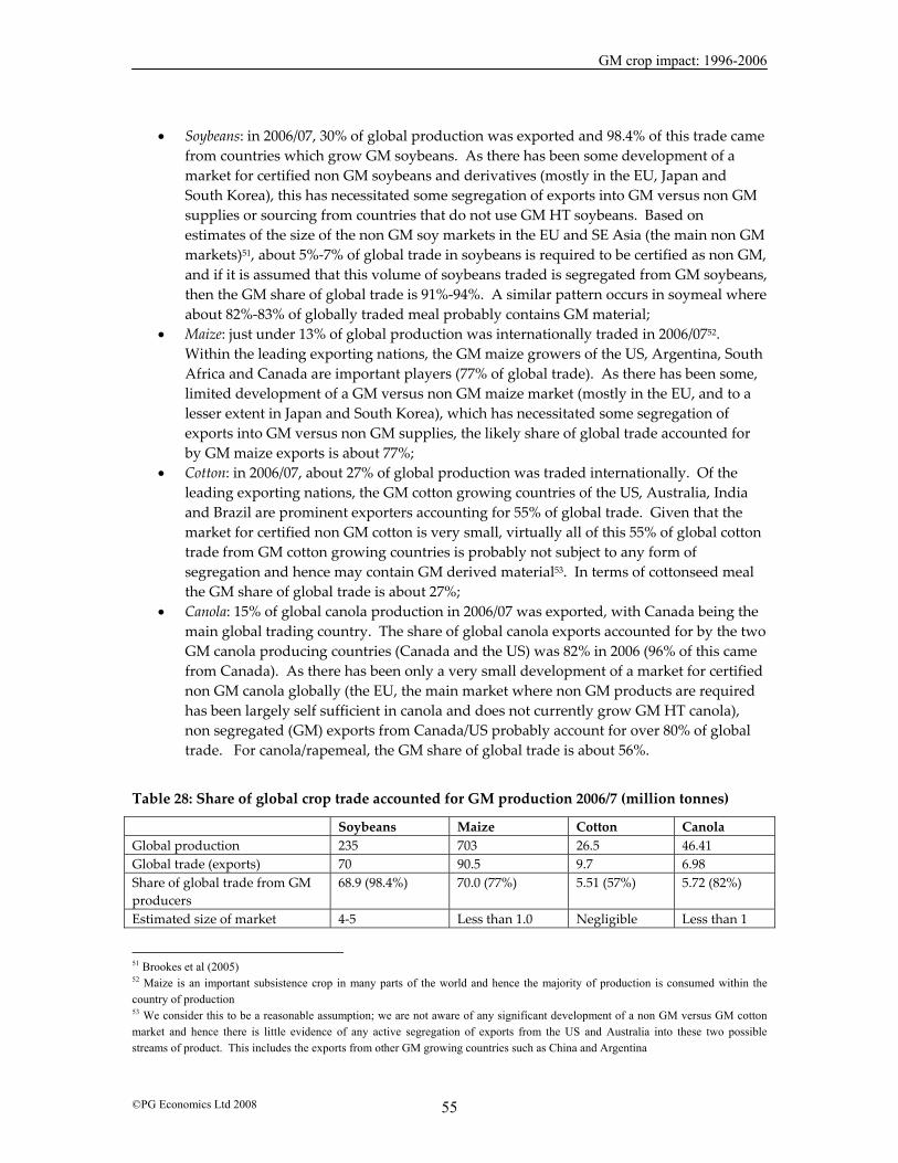
GM crop impact: 1996-2006
©PG Economics Ltd 2008 55
• Soybeans: in 2006/07, 30% of global production was exported and 98.4% of this trade came
from countries which grow GM soybeans. As there has been some development of a market for certified non GM soybeans and derivatives (mostly in the EU, Japan and South Korea), this has necessitated some segregation of exports into GM versus non GM supplies or sourcing from countries that do not use GM HT soybeans. Based on estimates of the size of the non GM soy markets in the EU and SE Asia (the main non GM markets)51, about 5%-7% of global trade in soybeans is required to be certified as non GM, and if it is assumed that this volume of soybeans traded is segregated from GM soybeans, then the GM share of global trade is 91%-94%. A similar pattern occurs in soymeal where about 82%-83% of globally traded meal probably contains GM material;
• Maize: just under 13% of global production was internationally traded in 2006/0752. Within the leading exporting nations, the GM maize growers of the US, Argentina, South Africa and Canada are important players (77% of global trade). As there has been some, limited development of a GM versus non GM maize market (mostly in the EU, and to a lesser extent in Japan and South Korea), which has necessitated some segregation of exports into GM versus non GM supplies, the likely share of global trade accounted for by GM maize exports is about 77%;
• Cotton: in 2006/07, about 27% of global production was traded internationally. Of the leading exporting nations, the GM cotton growing countries of the US, Australia, India and Brazil are prominent exporters accounting for 55% of global trade. Given that the market for certified non GM cotton is very small, virtually all of this 55% of global cotton trade from GM cotton growing countries is probably not subject to any form of segregation and hence may contain GM derived material53. In terms of cottonseed meal the GM share of global trade is about 27%;
• Canola: 15% of global canola production in 2006/07 was exported, with Canada being the main global trading country. The share of global canola exports accounted for by the two GM canola producing countries (Canada and the US) was 82% in 2006 (96% of this came from Canada). As there has been only a very small development of a market for certified non GM canola globally (the EU, the main market where non GM products are required has been largely self sufficient in canola and does not currently grow GM HT canola), non segregated (GM) exports from Canada/US probably account for over 80% of global trade. For canola/rapemeal, the GM share of global trade is about 56%.
Table 28: Share of global crop trade accounted for GM production 2006/7 (million tonnes)
Soybeans Maize Cotton Canola Global production 235 703 26.5 46.41 Global trade (exports) 70 90.5 9.7 6.98 Share of global trade from GM producers
68.9 (98.4%) 70.0 (77%) 5.51 (57%) 5.72 (82%)
Estimated size of market 4-5 Less than 1.0 Negligible Less than 1
51 Brookes et al (2005) 52 Maize is an important subsistence crop in many parts of the world and hence the majority of production is consumed within the country of production 53 We consider this to be a reasonable assumption; we are not aware of any significant development of a non GM versus GM cotton market and hence there is little evidence of any active segregation of exports from the US and Australia into these two possible streams of product. This includes the exports from other GM growing countries such as China and Argentina

GM crop impact: 1996-2006
©PG Economics Ltd 2008 56
requiring certified non GM (in countries that have import requirements) Estimated share of global trade that may contain GM (ie, not required to be segregated)
63.9-66.0 70 5.51 5.72
Share of global trade that may be GM
91%-94% 77% 57% 82%
Sources: derived from and updated - USDA & Oil World statistics, Brookes et al (2005) Notes: Estimated size of non GM market for soybeans (based primarly on demand for derivatives used mostly in the food industry): EU 4 million tonnes bean equivalents, Japan and South Korea 02-0.3 million tonnes
Table 29: Share of global crop derivative (meal) trade accounted for GM production 2006/7 (million tonnes)
Soymeal Cottonseed meal Canola/rape meal Global production 156 19.8 27.3 Global trade (exports) 54.7 0.51 2.94 Share of global trade from GM producers 48.38 (88%) 0.14 (27%) 1.66 (56%) Estimated size of market requiring certified non GM (in countries that have import requirements)
3-3.5 Negligible Negligible
Estimated share of global trade that may contain GM (ie, not required to be segregated)
44.88-45.38 0.14 1.66
Share of global trade that may be GM 82-83% 27% 56% Sources: derived from and updated - USDA & Oil World statistics, Brookes et al (2005) Notes: Estimated size of non GM market for soymeal: EU 3 million tonnes, Japan and South Korea 0.1-0.5 million tonnes (derived largely from certified non GM beans referred to in above table) c) Impact on prices Assessing the impact of the GM agronomic, cost saving technology such as herbicide tolerance and insect resistance on the prices of soybeans, maize, cotton and canola (and derivatives) is difficult. Current and past prices reflect a multitude of factors of which the introduction and adoption of new, cost saving technologies is one. This means that disaggregating the effect of different variables on prices is far from easy, and in the case of the impact of a single example of cost saving technology, it is virtually impossible. Whilst this means that it is not possible to be precise about the past/current impact of GM technology to date, the following comments and assessments can be made.
i) The real price of food and feed products has fallen consistently over the last 50 years. This has not come about ‘out of the blue’ but from enormous improvements in productivity by producers. These productivity improvements have arisen from the adoption of new technologies and techniques.
ii) In preceding sub-sections of this report, the extent of use of GM technology adoption
globally identified that:
• For soybeans the majority of both global production and trade is accounted for by GM production;

GM crop impact: 1996-2006
©PG Economics Ltd 2008 57
• For maize, cotton and canola, whilst the majority of global production is still non GM, the majority of globally traded produce contains materials derived from GM production.
This means for a crop such as soybeans, that GM production now effectively influences and sets the baseline price for commodity traded soybeans and derivatives on a global basis. Given that GM soybean varieties have provided significant cost savings and farm income gains (eg, $2.36 billion in 2006) to growers, it is likely that some of the benefits of the cost saving will have been passed on down the supply chain in the form of lower real prices for commodity traded soybeans. Thus, the current baseline price for all soybeans, including non-GM soy is probably at a lower real level than it would otherwise (in the absence of adoption of the technology) have been. A similar process of ‘transfer’ of some of the farm income benefits of using GM technology in the other three crops has also probably occurred, although to a lesser extent because of the lower penetration of global production and trade of GM in these crops.
Building on this theme of the impact of the technology to lower real soybean prices, some (limited) economic analysis has been undertaken to estimate the impact of GM technology on global prices of soybeans. Moschini et al (2000) estimated that by 2000 the influence of GM soybean technology on world prices of soybeans had been between -0.5% and -1%, and that as adoption levels increased this could increase up to -6% (if all global production was GM). Qaim & Traxler (2002) estimated the impact of RR soybean technology adoption on global soybean prices to have been -1.9% by 2001. Based on this analysis, it is therefore likely that currently the world price of soybeans is lower by between 2% and 6% than it might otherwise have been in the absence of GM technology. This benefit will have been dissipated through the post farm gate supply chain, with some of the gains having been passed onto consumers in the form of lower real prices.
• Whilst the additional volumes of food and fibre production arising from the positive yield effect of GM technology use (see a) above), suggest a small impact relative to global production, these volumes are far more significant in terms of global trade in these commodities (equal to +17% of global trade on soybeans, +11% of global trade in corn, +14%of global trade in cotton lint and +3% of global trade in canola). This means that global trade levels in these crops are probably significantly higher than the levels would have been in the absence of use of GM technology and, therefore, world prices of these traded crops in 2006, were probably lower than they would otherwise have been. In other words, GM technology is having an important impact on global supplies of these food, feed and fibre commodities and is making an important contribution to constraining the level of price increases that would have otherwise occurred in the last 2-3 years.
GM crop impact: 1996-2006
©PG Economics Ltd 2008 58
4 The environmental impact of GM crops This section examines the environmental impact of using GM crops over the last eleven years. The two key aspects of environmental impact explored are:
a. Impact on insecticide and herbicide use. b. Impact on carbon emissions.
These are presented in the sub-sections below.
4.1 Use of insecticides and herbicides The most common way in which changes in pesticide use on GM crops has been presented is in terms of the volumes (quantities) of pesticides applied. Whilst comparisons of total volumes of pesticide use in a crop production system can be a useful indicator of environmental impacts, it is an imperfect measure because:
• different active ingredients and amounts may be applied in GM or conventional systems; • the environmental behaviour and toxicity profile of individual pesticides varies.
To provide a more robust measurement of the environmental impact of GM crops, the analysis presented in the sub-sections below includes both an assessment of pesticide active ingredient use, as well as the assessment of the specific pesticides used via an indicator known as the Environmental Impact Quotient (EIQ). This universal indicator, developed by Kovach et al (1992 & updated annually), effectively integrates the various environmental impacts of individual pesticides into a single ‘field value per hectare’. This provides a more balanced assessment of the impact of GM crops on the environment as it draws on all of the key toxicity and environmental exposure data related to individual products (as applicable to impacts on farm workers, consumers and ecology) and hence provides not only a consistent but a fairly comprehensive measure of environmental impact. Readers should however note that the EIQ is an indicator only and therefore does not take into account all environmental issues/impacts. To provide a meaningful measure of environmental impact, the EIQ value is multiplied by the amount of pesticide active ingredient (ai) used per hectare to produce a field EIQ value. For example, the EIQ rating for glyphosate is 15.3. By using this rating multiplied by the amount of glyphosate used per hectare (eg, an hypothetical example of 1.1 kg applied per ha), the field EIQ value for glyphosate would be equivalent to 16.83/ha. The EIQ indicator used is therefore a comparison of the field EIQ/ha for conventional versus GM crop production systems, with the total environmental ‘foot print’ or load of each system, a direct function of respective field EIQ/ha values and the area planted to each type of production (GM versus non GM).
4.1.1 GM herbicide tolerant (to glyphosate) soybeans (GM HT) a) The USA
In examining the impact on herbicide usage in the US, two main sources of information have been drawn on: USDA (NASS) national pesticide usage data and private farm level pesticide usage survey data from DMR Kynetec. Based on these sources of information, the main features
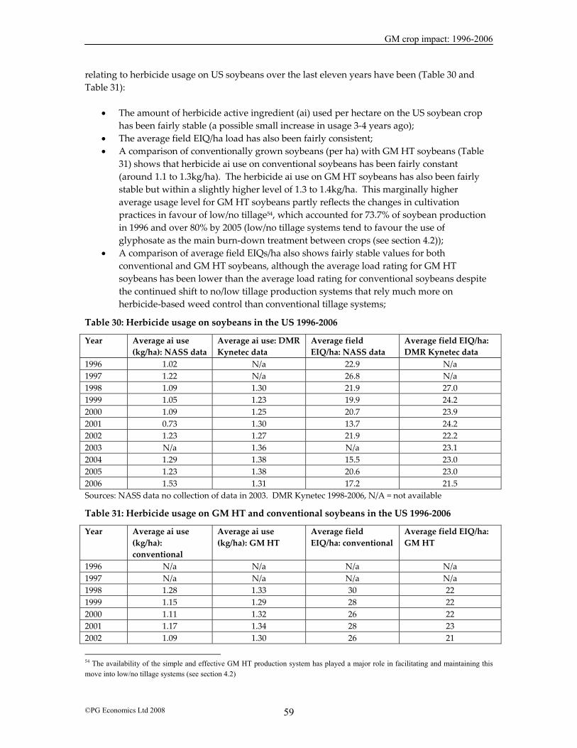
GM crop impact: 1996-2006
©PG Economics Ltd 2008 59
relating to herbicide usage on US soybeans over the last eleven years have been (Table 30 and Table 31):
• The amount of herbicide active ingredient (ai) used per hectare on the US soybean crop has been fairly stable (a possible small increase in usage 3-4 years ago);
• The average field EIQ/ha load has also been fairly consistent; • A comparison of conventionally grown soybeans (per ha) with GM HT soybeans (Table
31) shows that herbicide ai use on conventional soybeans has been fairly constant (around 1.1 to 1.3kg/ha). The herbicide ai use on GM HT soybeans has also been fairly stable but within a slightly higher level of 1.3 to 1.4kg/ha. This marginally higher average usage level for GM HT soybeans partly reflects the changes in cultivation practices in favour of low/no tillage54, which accounted for 73.7% of soybean production in 1996 and over 80% by 2005 (low/no tillage systems tend to favour the use of glyphosate as the main burn-down treatment between crops (see section 4.2));
• A comparison of average field EIQs/ha also shows fairly stable values for both conventional and GM HT soybeans, although the average load rating for GM HT soybeans has been lower than the average load rating for conventional soybeans despite the continued shift to no/low tillage production systems that rely much more on herbicide-based weed control than conventional tillage systems;
Table 30: Herbicide usage on soybeans in the US 1996-2006
Year Average ai use (kg/ha): NASS data
Average ai use: DMR Kynetec data
Average field EIQ/ha: NASS data
Average field EIQ/ha: DMR Kynetec data
1996 1.02 N/a 22.9 N/a 1997 1.22 N/a 26.8 N/a 1998 1.09 1.30 21.9 27.0 1999 1.05 1.23 19.9 24.2 2000 1.09 1.25 20.7 23.9 2001 0.73 1.30 13.7 24.2 2002 1.23 1.27 21.9 22.2 2003 N/a 1.36 N/a 23.1 2004 1.29 1.38 15.5 23.0 2005 1.23 1.38 20.6 23.0 2006 1.53 1.31 17.2 21.5 Sources: NASS data no collection of data in 2003. DMR Kynetec 1998-2006, N/A = not available
Table 31: Herbicide usage on GM HT and conventional soybeans in the US 1996-2006
Year Average ai use (kg/ha): conventional
Average ai use (kg/ha): GM HT
Average field EIQ/ha: conventional
Average field EIQ/ha: GM HT
1996 N/a N/a N/a N/a 1997 N/a N/a N/a N/a 1998 1.28 1.33 30 22 1999 1.15 1.29 28 22 2000 1.11 1.32 26 22 2001 1.17 1.34 28 23 2002 1.09 1.30 26 21
54 The availability of the simple and effective GM HT production system has played a major role in facilitating and maintaining this move into low/no tillage systems (see section 4.2)
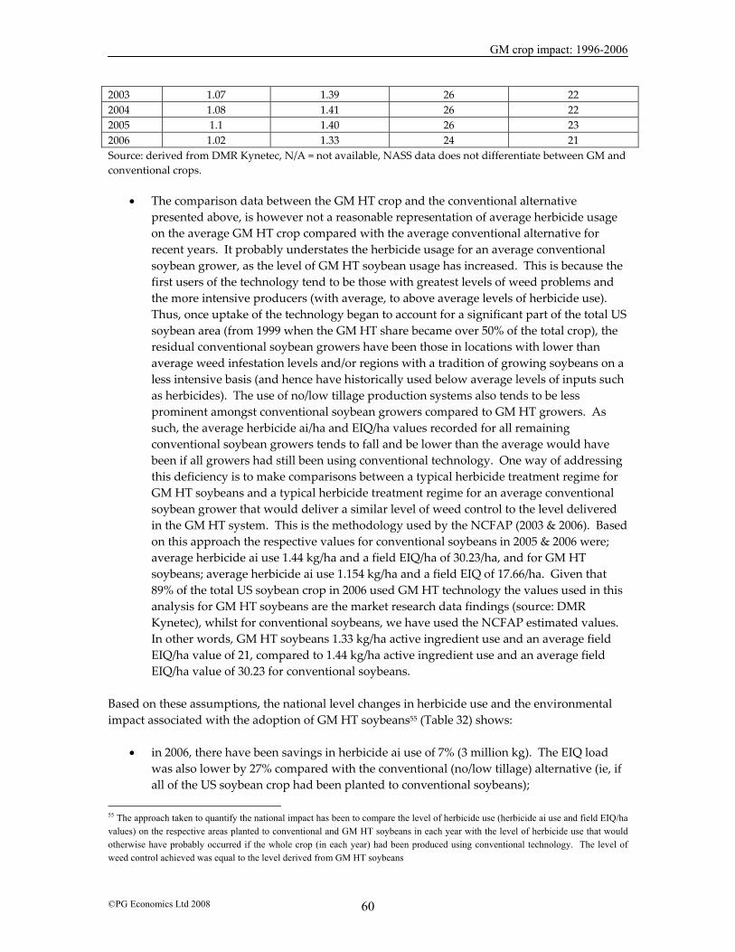
GM crop impact: 1996-2006
©PG Economics Ltd 2008 60
2003 1.07 1.39 26 22 2004 1.08 1.41 26 22 2005 1.1 1.40 26 23 2006 1.02 1.33 24 21 Source: derived from DMR Kynetec, N/A = not available, NASS data does not differentiate between GM and conventional crops.
• The comparison data between the GM HT crop and the conventional alternative presented above, is however not a reasonable representation of average herbicide usage on the average GM HT crop compared with the average conventional alternative for recent years. It probably understates the herbicide usage for an average conventional soybean grower, as the level of GM HT soybean usage has increased. This is because the first users of the technology tend to be those with greatest levels of weed problems and the more intensive producers (with average, to above average levels of herbicide use). Thus, once uptake of the technology began to account for a significant part of the total US soybean area (from 1999 when the GM HT share became over 50% of the total crop), the residual conventional soybean growers have been those in locations with lower than average weed infestation levels and/or regions with a tradition of growing soybeans on a less intensive basis (and hence have historically used below average levels of inputs such as herbicides). The use of no/low tillage production systems also tends to be less prominent amongst conventional soybean growers compared to GM HT growers. As such, the average herbicide ai/ha and EIQ/ha values recorded for all remaining conventional soybean growers tends to fall and be lower than the average would have been if all growers had still been using conventional technology. One way of addressing this deficiency is to make comparisons between a typical herbicide treatment regime for GM HT soybeans and a typical herbicide treatment regime for an average conventional soybean grower that would deliver a similar level of weed control to the level delivered in the GM HT system. This is the methodology used by the NCFAP (2003 & 2006). Based on this approach the respective values for conventional soybeans in 2005 & 2006 were; average herbicide ai use 1.44 kg/ha and a field EIQ/ha of 30.23/ha, and for GM HT soybeans; average herbicide ai use 1.154 kg/ha and a field EIQ of 17.66/ha. Given that 89% of the total US soybean crop in 2006 used GM HT technology the values used in this analysis for GM HT soybeans are the market research data findings (source: DMR Kynetec), whilst for conventional soybeans, we have used the NCFAP estimated values. In other words, GM HT soybeans 1.33 kg/ha active ingredient use and an average field EIQ/ha value of 21, compared to 1.44 kg/ha active ingredient use and an average field EIQ/ha value of 30.23 for conventional soybeans.
Based on these assumptions, the national level changes in herbicide use and the environmental impact associated with the adoption of GM HT soybeans55 (Table 32) shows:
• in 2006, there have been savings in herbicide ai use of 7% (3 million kg). The EIQ load was also lower by 27% compared with the conventional (no/low tillage) alternative (ie, if all of the US soybean crop had been planted to conventional soybeans);
55 The approach taken to quantify the national impact has been to compare the level of herbicide use (herbicide ai use and field EIQ/ha values) on the respective areas planted to conventional and GM HT soybeans in each year with the level of herbicide use that would otherwise have probably occurred if the whole crop (in each year) had been produced using conventional technology. The level of weed control achieved was equal to the level derived from GM HT soybeans
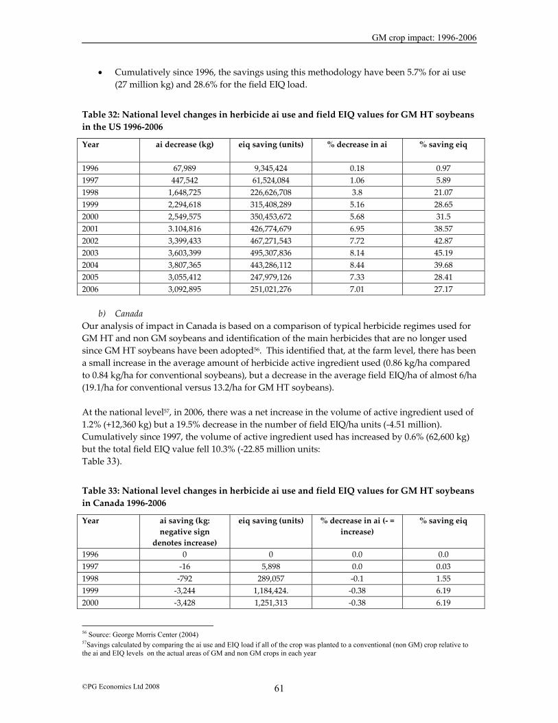
GM crop impact: 1996-2006
©PG Economics Ltd 2008 61
• Cumulatively since 1996, the savings using this methodology have been 5.7% for ai use (27 million kg) and 28.6% for the field EIQ load.
Table 32: National level changes in herbicide ai use and field EIQ values for GM HT soybeans in the US 1996-2006
Year ai decrease (kg) eiq saving (units) % decrease in ai % saving eiq
1996 67,989 9,345,424 0.18 0.97 1997 447,542 61,524,084 1.06 5.89 1998 1,648,725 226,626,708 3.8 21.07 1999 2,294,618 315,408,289 5.16 28.65 2000 2,549,575 350,453,672 5.68 31.5 2001 3.104,816 426,774,679 6.95 38.57 2002 3,399,433 467,271,543 7.72 42.87 2003 3,603,399 495,307,836 8.14 45.19 2004 3,807,365 443,286,112 8.44 39.68 2005 3,055,412 247,979,126 7.33 28.41 2006 3,092,895 251,021,276 7.01 27.17
b) Canada Our analysis of impact in Canada is based on a comparison of typical herbicide regimes used for GM HT and non GM soybeans and identification of the main herbicides that are no longer used since GM HT soybeans have been adopted56. This identified that, at the farm level, there has been a small increase in the average amount of herbicide active ingredient used (0.86 kg/ha compared to 0.84 kg/ha for conventional soybeans), but a decrease in the average field EIQ/ha of almost 6/ha (19.1/ha for conventional versus 13.2/ha for GM HT soybeans). At the national level57, in 2006, there was a net increase in the volume of active ingredient used of 1.2% (+12,360 kg) but a 19.5% decrease in the number of field EIQ/ha units (-4.51 million). Cumulatively since 1997, the volume of active ingredient used has increased by 0.6% (62,600 kg) but the total field EIQ value fell 10.3% (-22.85 million units: Table 33).
Table 33: National level changes in herbicide ai use and field EIQ values for GM HT soybeans in Canada 1996-2006
Year ai saving (kg: negative sign
denotes increase)
eiq saving (units) % decrease in ai (- = increase)
% saving eiq
1996 0 0 0.0 0.0 1997 -16 5,898 0.0 0.03 1998 -792 289,057 -0.1 1.55 1999 -3,244 1,184,424. -0.38 6.19 2000 -3,428 1,251,313 -0.38 6.19
56 Source: George Morris Center (2004) 57Savings calculated by comparing the ai use and EIQ load if all of the crop was planted to a conventional (non GM) crop relative to the ai and EIQ levels on the actual areas of GM and non GM crops in each year
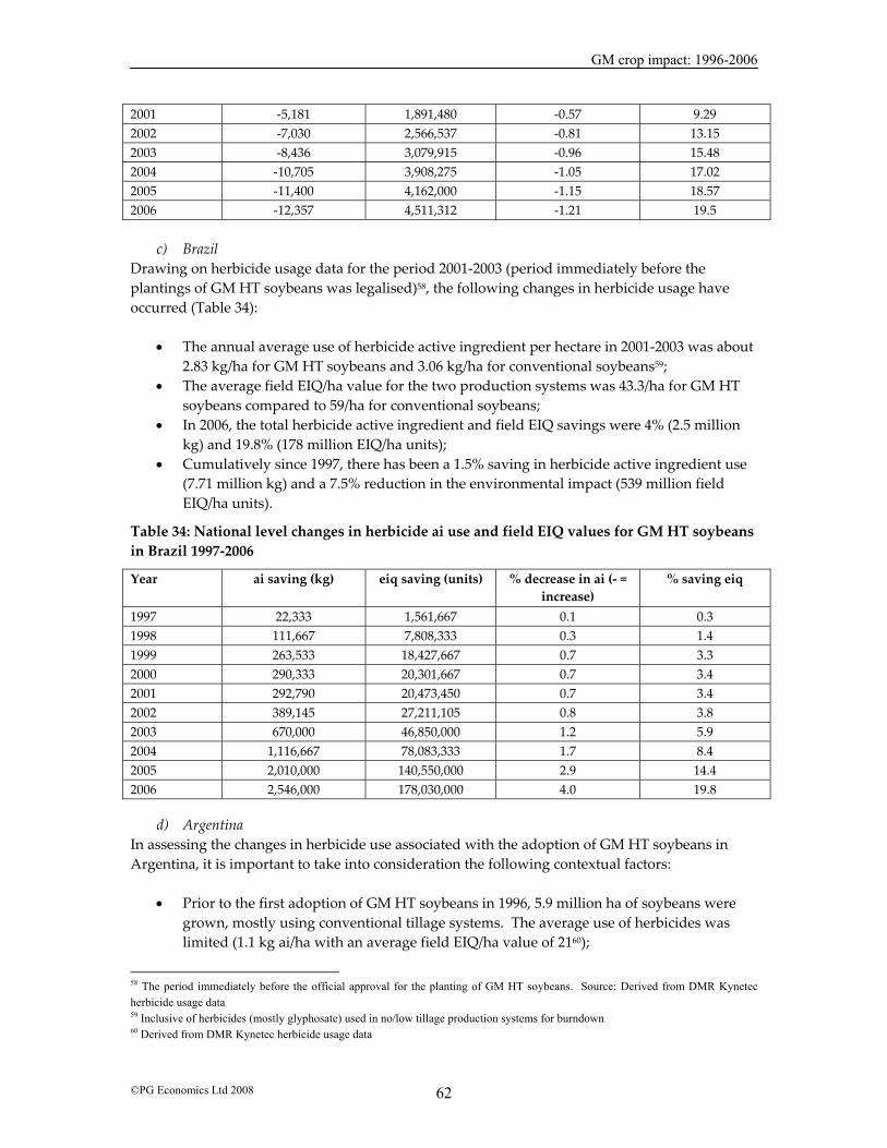
GM crop impact: 1996-2006
©PG Economics Ltd 2008 62
2001 -5,181 1,891,480 -0.57 9.29 2002 -7,030 2,566,537 -0.81 13.15 2003 -8,436 3,079,915 -0.96 15.48 2004 -10,705 3,908,275 -1.05 17.02 2005 -11,400 4,162,000 -1.15 18.57 2006 -12,357 4,511,312 -1.21 19.5
c) Brazil Drawing on herbicide usage data for the period 2001-2003 (period immediately before the plantings of GM HT soybeans was legalised)58, the following changes in herbicide usage have occurred (Table 34):
• The annual average use of herbicide active ingredient per hectare in 2001-2003 was about 2.83 kg/ha for GM HT soybeans and 3.06 kg/ha for conventional soybeans59;
• The average field EIQ/ha value for the two production systems was 43.3/ha for GM HT soybeans compared to 59/ha for conventional soybeans;
• In 2006, the total herbicide active ingredient and field EIQ savings were 4% (2.5 million kg) and 19.8% (178 million EIQ/ha units);
• Cumulatively since 1997, there has been a 1.5% saving in herbicide active ingredient use (7.71 million kg) and a 7.5% reduction in the environmental impact (539 million field EIQ/ha units).
Table 34: National level changes in herbicide ai use and field EIQ values for GM HT soybeans in Brazil 1997-2006
Year ai saving (kg) eiq saving (units) % decrease in ai (- = increase)
% saving eiq
1997 22,333 1,561,667 0.1 0.3 1998 111,667 7,808,333 0.3 1.4 1999 263,533 18,427,667 0.7 3.3 2000 290,333 20,301,667 0.7 3.4 2001 292,790 20,473,450 0.7 3.4 2002 389,145 27,211,105 0.8 3.8 2003 670,000 46,850,000 1.2 5.9 2004 1,116,667 78,083,333 1.7 8.4 2005 2,010,000 140,550,000 2.9 14.4 2006 2,546,000 178,030,000 4.0 19.8
d) Argentina In assessing the changes in herbicide use associated with the adoption of GM HT soybeans in Argentina, it is important to take into consideration the following contextual factors:
• Prior to the first adoption of GM HT soybeans in 1996, 5.9 million ha of soybeans were grown, mostly using conventional tillage systems. The average use of herbicides was limited (1.1 kg ai/ha with an average field EIQ/ha value of 2160);
58 The period immediately before the official approval for the planting of GM HT soybeans. Source: Derived from DMR Kynetec herbicide usage data 59 Inclusive of herbicides (mostly glyphosate) used in no/low tillage production systems for burndown 60 Derived from DMR Kynetec herbicide usage data
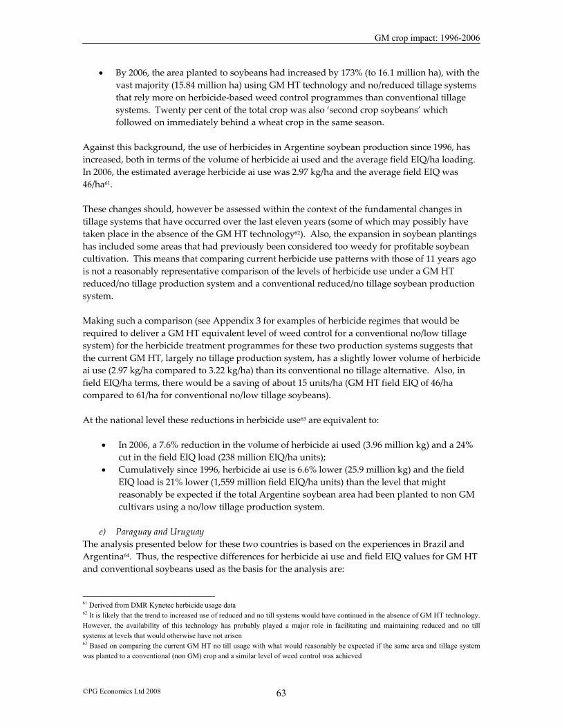
GM crop impact: 1996-2006
©PG Economics Ltd 2008 63
• By 2006, the area planted to soybeans had increased by 173% (to 16.1 million ha), with the vast majority (15.84 million ha) using GM HT technology and no/reduced tillage systems that rely more on herbicide-based weed control programmes than conventional tillage systems. Twenty per cent of the total crop was also ‘second crop soybeans’ which followed on immediately behind a wheat crop in the same season.
Against this background, the use of herbicides in Argentine soybean production since 1996, has increased, both in terms of the volume of herbicide ai used and the average field EIQ/ha loading. In 2006, the estimated average herbicide ai use was 2.97 kg/ha and the average field EIQ was 46/ha61. These changes should, however be assessed within the context of the fundamental changes in tillage systems that have occurred over the last eleven years (some of which may possibly have taken place in the absence of the GM HT technology62). Also, the expansion in soybean plantings has included some areas that had previously been considered too weedy for profitable soybean cultivation. This means that comparing current herbicide use patterns with those of 11 years ago is not a reasonably representative comparison of the levels of herbicide use under a GM HT reduced/no tillage production system and a conventional reduced/no tillage soybean production system. Making such a comparison (see Appendix 3 for examples of herbicide regimes that would be required to deliver a GM HT equivalent level of weed control for a conventional no/low tillage system) for the herbicide treatment programmes for these two production systems suggests that the current GM HT, largely no tillage production system, has a slightly lower volume of herbicide ai use (2.97 kg/ha compared to 3.22 kg/ha) than its conventional no tillage alternative. Also, in field EIQ/ha terms, there would be a saving of about 15 units/ha (GM HT field EIQ of 46/ha compared to 61/ha for conventional no/low tillage soybeans). At the national level these reductions in herbicide use63 are equivalent to:
• In 2006, a 7.6% reduction in the volume of herbicide ai used (3.96 million kg) and a 24% cut in the field EIQ load (238 million EIQ/ha units);
• Cumulatively since 1996, herbicide ai use is 6.6% lower (25.9 million kg) and the field EIQ load is 21% lower (1,559 million field EIQ/ha units) than the level that might reasonably be expected if the total Argentine soybean area had been planted to non GM cultivars using a no/low tillage production system.
e) Paraguay and Uruguay
The analysis presented below for these two countries is based on the experiences in Brazil and Argentina64. Thus, the respective differences for herbicide ai use and field EIQ values for GM HT and conventional soybeans used as the basis for the analysis are:
61 Derived from DMR Kynetec herbicide usage data 62 It is likely that the trend to increased use of reduced and no till systems would have continued in the absence of GM HT technology. However, the availability of this technology has probably played a major role in facilitating and maintaining reduced and no till systems at levels that would otherwise have not arisen 63 Based on comparing the current GM HT no till usage with what would reasonably be expected if the same area and tillage system was planted to a conventional (non GM) crop and a similar level of weed control was achieved
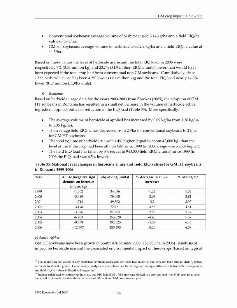
GM crop impact: 1996-2006
©PG Economics Ltd 2008 64
• Conventional soybeans: average volume of herbicide used 3.14 kg/ha and a field EIQ/ha
value of 59.8/ha; • GM HT soybeans: average volume of herbicide used 2.9 kg/ha and a field EIQ/ha value of
44.5/ha. Based on these values the level of herbicide ai use and the total EIQ load, in 2006 were respectively 7% (0.54 million kg) and 23.7% (34.9 million EIQ/ha units) lower than would have been expected if the total crop had been conventional non GM soybeans. Cumulatively, since 1999, herbicide ai use has been 4.2% lower (1.81 million kg) and the total EIQ load nearly 14.3% lower (81.7 million EIQ/ha units).
f) Romania Based on herbicide usage data for the years 2000-2003 from Brookes (2005), the adoption of GM HT soybeans in Romania has resulted in a small net increase in the volume of herbicide active ingredient applied, but a net reduction in the EIQ load (Table 35). More specifically:
• The average volume of herbicide ai applied has increased by 0.09 kg/ha from 1.26 kg/ha to 1.35 kg/ha);
• The average field EIQ/ha has decreased from 23/ha for conventional soybeans to 21/ha for GM HT soybeans;
• The total volume of herbicide ai use65 is 4% higher (equal to about 42,000 kg) than the level of use if the crop had been all non GM since 1999 (in 2006 usage was 5.25% higher);
• The field EIQ load has fallen by 5% (equal to 943,000 field EIQ/ha units) since 1999 (in 2006 the EIQ load was 6.5% lower).
Table 35: National level changes in herbicide ai use and field EIQ values for GM HT soybeans in Romania 1999-2006
Year Ai use (negative sign denotes an increase
in use: kg)
eiq saving (units) % decrease in ai (- = increase)
% saving eiq
1999 -1,502 34,016 -1.22 1.52 2000 -3,489 79,005 -3.06 3.81 2001 -1,744 39,502 -3.2 3.97 2002 -3,198 72,421 -3.55 4.41 2003 -3,876 87,783 -2.53 3.14 2004 -6,783 153,620 -4.48 5.57 2005 -8,479 192,025 -5.59 6.45 2006 -12,597 285,295 -5.25 6.53 g) South Africa GM HT soybeans have been grown in South Africa since 2000 (150,000 ha in 2006). Analysis of impact on herbicide use and the associated environmental impact of these crops (based on typical
64 The authors are not aware of any published herbicide usage data for these two countries and have not been able to identify typical herbicide treatment regimes. Consequently, analysis has been based on the average of findings (differences between the average ai/ha and field EIQ/ha values in Brazil and Argentina) 65 Savings calculated by comparing the ai use and EIQ load if all of the crop was planted to a conventional (non GM) crop relative to the ai and EIQ levels based on the actual areas of GM and non GM crops in each year

GM crop impact: 1996-2006
©PG Economics Ltd 2008 65
herbicide treatment regimes for GM HT soybeans and conventional soybeans: see Appendix 3) shows the following:
• Since 1999, the total volume of herbicide ai use has been 4.4% higher (equal to about 69,000 kg of ai) than the level of use if the crop had been all non GM (in 2006 usage was 7.3% higher);
• The field EIQ load has fallen by 8.1 (equal to about 2.7 million field EIQ/ha units) since 1999 (in 2006 the EIQ load was 13.4% lower).
h) Summary of impact Across all of the countries that have adopted GM HT soybeans since 1996, the net impact on herbicide use and the associated environmental impact66 has been (Figure 15):
• In 2006, a 6% decrease in the total volume of herbicide ai applied (10.1 million kg) and a 23.7% reduction in the environmental impact (measured in terms of the field EIQ/ha load);
• Since 1996, 4.4% less herbicide ai has been used (62 million kg) and the environmental impact applied to the soybean crop has fallen by 20.4%.
This suggests that over the period 1996-2006, there has been a significant net environmental gain directly associated with the application of the GM HT technology. This level of net environmental benefit has been increasing as the area planted to GM HT soybeans has expanded.
Figure 15: Reduction in herbicide use and the environmental load from using GM HT soybeans in all adopting countries 1996-2006
66 Relative to the expected herbicide usage if all of the GM HT area had been planted to conventional varieties, using the same tillage system (largely no/low till) and delivering an equal level of weed control to that obtained under the GM HT system
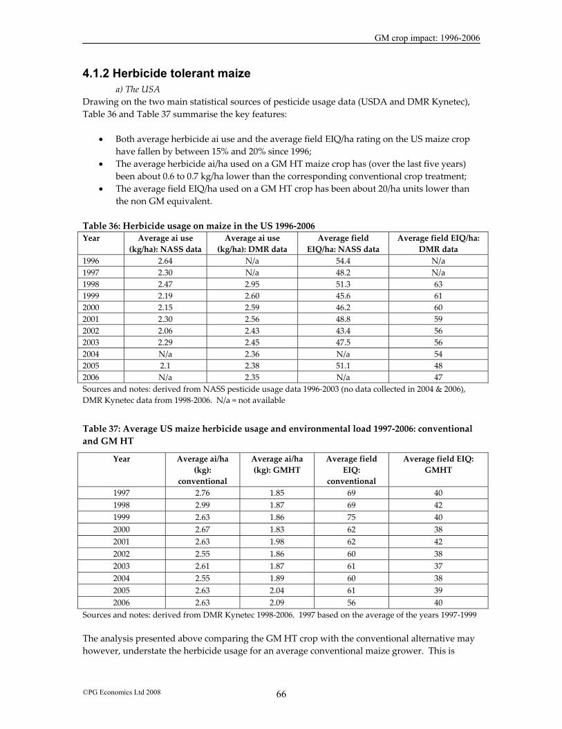
GM crop impact: 1996-2006
©PG Economics Ltd 2008 66
4.1.2 Herbicide tolerant maize a) The USA
Drawing on the two main statistical sources of pesticide usage data (USDA and DMR Kynetec), Table 36 and Table 37 summarise the key features:
• Both average herbicide ai use and the average field EIQ/ha rating on the US maize crop have fallen by between 15% and 20% since 1996;
• The average herbicide ai/ha used on a GM HT maize crop has (over the last five years) been about 0.6 to 0.7 kg/ha lower than the corresponding conventional crop treatment;
• The average field EIQ/ha used on a GM HT crop has been about 20/ha units lower than the non GM equivalent.
Table 36: Herbicide usage on maize in the US 1996-2006 Year Average ai use
(kg/ha): NASS data Average ai use
(kg/ha): DMR data Average field
EIQ/ha: NASS data Average field EIQ/ha:
DMR data 1996 2.64 N/a 54.4 N/a 1997 2.30 N/a 48.2 N/a 1998 2.47 2.95 51.3 63 1999 2.19 2.60 45.6 61 2000 2.15 2.59 46.2 60 2001 2.30 2.56 48.8 59 2002 2.06 2.43 43.4 56 2003 2.29 2.45 47.5 56 2004 N/a 2.36 N/a 54 2005 2.1 2.38 51.1 48 2006 N/a 2.35 N/a 47 Sources and notes: derived from NASS pesticide usage data 1996-2003 (no data collected in 2004 & 2006), DMR Kynetec data from 1998-2006. N/a = not available
Table 37: Average US maize herbicide usage and environmental load 1997-2006: conventional and GM HT
Year Average ai/ha (kg):
conventional
Average ai/ha (kg): GMHT
Average field EIQ:
conventional
Average field EIQ: GMHT
1997 2.76 1.85 69 40 1998 2.99 1.87 69 42 1999 2.63 1.86 75 40 2000 2.67 1.83 62 38 2001 2.63 1.98 62 42 2002 2.55 1.86 60 38 2003 2.61 1.87 61 37 2004 2.55 1.89 60 38 2005 2.63 2.04 61 39 2006 2.63 2.09 56 40
Sources and notes: derived from DMR Kynetec 1998-2006. 1997 based on the average of the years 1997-1999 The analysis presented above comparing the GM HT crop with the conventional alternative may however, understate the herbicide usage for an average conventional maize grower. This is

GM crop impact: 1996-2006
©PG Economics Ltd 2008 67
because the first users of the technology tend to be those with greatest levels of weed problems and more intensive producers, with average to above average levels of herbicide use. Also, as the uptake of the technology increases, the residual conventional maize growers tend to be those with lower than average weed infestation levels and/or with a tradition of growing maize on an extensive basis (and hence have historically used below average levels of inputs such as herbicides). The extent to which average herbicide use for conventional maize growers may be understated is nevertheless, likely to have been less important than in soybeans (or cotton) in the US, because of the relatively lower levels of GM HT adoption in the US maize crop to date (36% of the total crop in 2006). Analysis by the NCFAP (2003 & 2006) compared typical herbicide treatment regimes for GM HT and average conventional maize crops that would deliver similar levels of weed control to that level delivered in the GM HT systems. This identified (for 2005) average values for conventional maize of 3.64 kg herbicide ai/ha and a field EIQ rating of 80.61/ha (mix of herbicides such as metalochlor, atrazine, mesotrione, nicosulfuron and rimsulfuron). This compares with GM glyphosate tolerant maize (2.8 kg herbicide ai/ha and a field EIQ rating of 55.36/ha (use of glyphosate plus half doses of metalochlor and atrazine relative to conventional crops)) and GM glufosinate tolerant maize (2.24 kg herbicide ai/ha and a field EIQ/ha rating of 52.89/ha). At the national level (Table 38), in 2006, there has been an annual saving in the volume of herbicide active ingredient use of 8.9% (10.2 million kg). The annual field EIQ load on the US maize crop has also fallen by about 11.4% in 2006 (equal to 292 million field EIQ/ha units). The cumulative decrease in active ingredient use since 1997 has been 3.9 (44.5 million kg), and the cumulative reduction in the field EIQ load has been 4.7%.
Table 38: National level changes in herbicide ai use and field EIQ values for GM HT maize in the US 1997-2006
Year ai decrease (kg)
eiq saving (units) % decrease in ai % saving eiq
1997 150,669 2,838,353 0.15 0.14 1998 2,035,698 40,343,821 2.03 1.95 1999 1,691,777 36,734,004 1.75 1.84 2000 2,637,395 55,881,629 2.65 2.73 2001 2,733,427 62,108,932 2.88 3.18 2002 4,227,123 97,545,980 4.28 4.80 2003 5,226,766 121,853,076 5.31 6.01 2004 7,918,178 183,818,420 6.52 7.39 2005 7,658,532 220,002,711 6.39 8.25 2006 10,211,283 291,999,309 8.9 11.43
b) Canada The impact on herbicide use in the Canadian maize crop has been similar to the impact reported above in the US. Using industry sourced information67 about typical herbicide regimes for conventional and GM herbicide tolerant maize (see Appendix 3), the key impact findings are:
67 Including the Weed Control Guide (2004 and updated) from the Departments’ of Agriculture in Ontario, Manitoba and Saskatchewan (available on the Canola Council’s web-site www.canola-council.org)

GM crop impact: 1996-2006
©PG Economics Ltd 2008 68
• The herbicide ai/ha load on a GM HT crop has been between 0.88 kg/ha (GM glyphosate
tolerant) and 1.069 kg/ha (GM glufosinate tolerant) lower than the conventional maize equivalent crop (average herbicide ai use at 2.71 kg/ha);
• The field EIQ/ha values for GM glyphosate and GM glufosinate tolerant maize are respectively 37/ha and 39/ha compared to 62/ha for conventional maize;
• At the national level in 2006 (based on the plantings of the different production systems), the reductions in herbicide ai use and the total field EIQ load were respectively 16.9% (500,000 kg) and 19% (12.8 million: Table 39);
• Cumulatively since 1997, total national herbicide ai use has fallen by 7.8% (1.99 million kg) and the total EIQ load has fallen by 8.4% (48.8 million field EIQ units).
Table 39: Change in herbicide use and environmental load from using GM HT maize in Canada 1999-2006 Year Total active ingredient saving
(kg) Total field EIQ reductions (in units per hectare)
1999 59,176 1,324,689 2000 121,676 2,777,245 2001 177,444 4,143,290 2002 254,643 6,015,394 2003 208,998 5,110,911 2004 202,771 5,060,887 2005 465,835 11,520,577 2006 500,098 12,831,445 Total 1,990,641 48,784,438
c) South Africa Drawing on industry level sources that compare typical herbicide treatment regimes for conventional and GM HT maize in South Africa (see appendix 3), the impact of using GM HT technology in the South African maize crop (269,000 ha in 2006) has been:
• On a per hectare basis, there has been a 0.257 kg decrease in the amount of herbicide active ingredient used and an improvement in the average field EIQ of 18.8/ha;
• In 2006, at the national level, the amount of herbicide used was 69,130 kgs (-1.5%) lower than the amount that would probably have been used if the crop had all been planted to conventional seed. The total field EIQ load was 5.1% lower;
• Cumulatively since 2003, total national herbicide ai use has fallen by 0.5% (85,860 kg) and the total EIQ load has fallen by 1.6%.
d) Argentina
Similar reductions in herbicide use and the environmental ‘foot print’, associated with the adoption of GM HT maize have been found in Argentina where this technology was first used in 2004 (see Appendix 3):
• The average volume of herbicide ai applied to GM HT maize has been 2.55kg/ha compared to 2.93 kg/ha for conventional maize;
• the average field EIQ/ha load for GM HT maize is significantly lower than the conventional counterpart (46/ha for GM HT maize, 59/ha for conventional maize);

GM crop impact: 1996-2006
©PG Economics Ltd 2008 69
• the reduction in the volume of herbicide used was 83,500 kg (-1%) in 2006. Since 2004, the cumulative reduction in usage has been 0.5% (- 115,000 kg);
• in terms of the field EIQ load, the reduction in 2006 was 1.7% (-2.85 million field/ha units) and over the period 2004-2006, the load factor fell by 0.9%.
e) Other countries GM HT maize was also grown commercially in the Philippines, for the first time in 2006 (30,675 ha). Weed control practices in maize in the Philippines are based on a combination of use of herbicides and hand weeding. The authors are not aware of any analysis which has examined the impact on herbicide use and the associated environmental ‘footprint’ of using GM HT maize in the Philippines. d) Summary of impact In the countries where GM HT maize has been most widely adopted, there has been a net decrease in both the volume of herbicides applied to maize and a net reduction in the environmental impact applied to the crop (Figure 16). More specifically:
• In 2006, total herbicide ai use was 8.3% lower (10.9 million kg) than the level of use if the total crop had been planted to conventional non GM (HT) varieties. The EIQ load was also lower by 10.8%;
• Cumulatively since 1997, the volume of herbicide ai applied is 3.9% lower than its conventional equivalent (a saving of 46.7 million kg). The EIQ load has been reduced by 4.6%.
Figure 16: Reduction in herbicide use and the environmental load from using GM HT maize in adopting countries 1997-2006

GM crop impact: 1996-2006
©PG Economics Ltd 2008 70
4.1.3 Herbicide tolerant cotton a) The USA
Drawing on the herbicide usage data from the USDA and DMR Kynetec, both the volume of ai used and the average field EIQ/ha on the US cotton crop has remained fairly stable over the last eleven years (Table 40).
Table 40: Herbicide usage on cotton in the US 1996-2006
Year Average ai use (kg/ha): NASS data
Average ai use (kg/ha): Doane data
Average field EIQ/ha: NASS data
Average field EIQ/ha: Doane data
1996 1.98 N/a 39.2 N/a 1997 2.43 N/a 51.8 N/a 1998 2.14 2.25 41.3 53.6 1999 2.18 2.06 41.9 45.5 2000 2.18 2.21 39.4 47.4 2001 1.89 2.34 34.2 46.3 2002 N/a 2.29 N/a 45.1 2003 2.27 2.30 37.9 43.5 2004 N/a 2.49 N/a 46.0 2005 N/p 2.60 N/p 46.0 2006 N/a 2.53 N/a 47.5 Sources and notes: derived from NASS pesticide usage data 1996-2003 (no data collected in 2002, 2004 & 2006), DMR Kynetec data from 1998-2006. N/p = Not presented - 2005 results based on NASS data are significantly different and inconsistent with previous trends and DMR data. These results have therefore not been presented Looking at a comparison of average usage data for GM HT versus conventional cotton, the DMR Kynetec dataset68 shows that the average level of herbicide ai use (per ha) has been consistently higher than the average level of usage on conventional cotton. In terms of the average field EIQ/ha, the DMR dataset suggests that there has been a marginally lower average field EIQ rating for GM HT cotton in the years 1997 to 2000, but since 2000, the average field EIQ/ha rating has been lower for conventional cotton (Table 41).
Table 41: Herbicide usage and its associated environmental load: GM HT and conventional cotton in the US 1997-2006
Year Average ai use (kg/ha): conventional cotton
Average ai use (kg/ha): GM HT cotton
Average field EIQ/ha: conventional cotton
Average field EIQ/ha: GM HT cotton
1997 2.1 2.38 48 46 1998 2.27 2.52 52 51 1999 1.92 2.27 44 43 2000 2.11 2.34 49 44 2001 1.93 2.51 45 47 2002 1.87 2.50 43 46 2003 1.65 2.53 37 46 2004 1.63 2.71 36 49 2005 1.60 2.79 36 50
68 The NASS dataset does allow for comparisons between the two types of production systems

GM crop impact: 1996-2006
©PG Economics Ltd 2008 71
2006 1.74 2.69 36 49 Sources and notes: derived from DMR 1998-2006. 1997 based on the average of the years 1997-1999 The reader should, however note that this comparison between the GM HT crop and the conventional alternative is not a representative comparison of the average GM HT crop with the average conventional alternative and probably understates the herbicide usage for an average conventional cotton grower, especially as the level of GM HT cotton usage has increased. This is because the first users of the technology were those with greatest levels of weed problems and more intensive producers, with average to above average levels of herbicide use. Also, once uptake of the technology began to account for a significant part of the total US cotton area (from 1999 when the GM HT share became over 40% of the total crop), the residual conventional cotton growers have been those in locations with lower than average weed infestation levels and/or regions with a tradition of growing cotton on an extensive basis (and hence have historically used below average levels of inputs such as herbicides, eg, West Texas). As such, the average herbicide ai/ha and EIQ/ha values recorded for all remaining conventional cotton growers tends to fall and be lower than the average would have been if all growers had still been using conventional technology. One way of addressing this deficiency is to make comparisons between a typical herbicide treatment regime for GM HT and a typical herbicide treatment regime for an average conventional cotton grower that would deliver a similar level of weed control to that level delivered in the GM HT system in the same location. This is the methodology used by the NCFAP (2003 and 2006). Based on this approach the respective values in 2005 and 2006 were, for conventional cotton, average herbicide ai use 5.69 kg/ha and a field EIQ/ha of 131/ha, and for GM GT cotton, herbicide ai use 3.94 kg/ha and a field EIQ of 90.5/ha. Given that these values are significantly higher than the average values for use across the US cotton in any year (see Table 41), we have therefore adjusted these values downwards to reflect the difference between the values for GM HT cotton identified by the NCFAP approach and the recorded usage data from DMR Kynetec. On this basis, the comparison level of usage recorded (and used in the national level analysis below) is, for example in 2006:
• conventional cotton average, herbicide ai use 3.88 kg/ha and a field EIQ/ha of 70.43/ha; • GM HT cotton, herbicide ai use 2.69 kg/ha and a field EIQ of 48.6/ha.
At the national level (Table 42), the impact of using the GM HT technology equates to 19.9% and 20.15% savings respectively in ai use and the field EIQ value for 2006. Cumulatively since 1997, the savings using this methodology have been 15% for ai use (31.3 million kg) and 15% (586 million field EIQ units).
Table 42: National level changes in herbicide ai use and field EIQ values for GM HT cotton in the US 1997-2006
Year ai decrease (kg)
eiq saving (units) % decrease in ai % saving eiq
1997 621,950 12,228,801 3.2 3.25 1998 1,583,599 32,405,044 8.0 8.12 1999 2,545,519 49,401,997 12.9 13.05 2000 2,991,420 57,357,218 14.1 14.26

GM crop impact: 1996-2006
©PG Economics Ltd 2008 72
2001 3,969,123 75,283,178 17.2 17.36 2002 3,743,505 69,615,866 17.8 17.98 2003 3,209,032 59,226,448 18.1 18.29 2004 3,802,134 69,357,168 18.4 18.60 2005 4,086,560 73,894,879 18.7 18.91 2006 4,782,882 87,715,834 19.9 20.15
b) Australia Drawing on information from the University of New England study from 200369, analysis of the typical herbicide treatment regimes for GM HT and conventional cotton (see Appendix 3) shows the following:
• The herbicide ai/ha load on a GM HT crop has been about 0.11 kg/ha higher (at 2.87 kg/ha) than the conventional cotton equivalent crop (2.77 kg/ha);
• The average field EIQ/ha value for GM HT cotton has been 51/ha compared to 66/ha for conventional cotton;
• At the national level (Table 43), in 2006 (based on the plantings of the different production systems), herbicide ai use has been 2.7% higher (11,190 kg) than the level expected if the whole crop had been planted to non GM cotton cultivars. The total field EIQ load was, however 15.6% lower;
• Cumulatively since 2000, total national herbicide ai use has increased by 0.8% (81,170 kg) although the total EIQ load had fallen by 4.4%.
Table 43: National level changes in herbicide ai use and field EIQ values for GM HT cotton in Australia 2000-2006 (negative sign denotes increase in use)
Year ai increase (kg)
eiq saving (units) % change in ai % saving eiq
2000 -1,290 178,358 -0.1 0.5 2001 -8,051 1,113,148 -0.8 4.8 2002 -9,756 1,348,907 -1.5 8.9 2003 -9,028 1,248,239 -1.7 9.7 2004 -17,624 2,436,743 -2.0 11.8 2005 -24,235 3,350,739 -2.9 16.6 2006 -11,187 1,546,699 -2.7 15.6
c) South Africa Using industry level sources that compare typical herbicide treatment regimes for conventional and GM HT cotton in South Africa (see appendix 3), the impact of using GM HT technology in the South African cotton crop has been:
• there has been an average 0.127 kg increase in the amount of herbicide active ingredient used (-8% increasing to an average of 1.8 kg/ha) but a 28% decrease in the environmental impact, as measured by the EIQ indicator (-10.7 field EIQ/ha units);
• In 2006, at the national level, the amount of herbicide used was1,180 kgs (+3.5%) higher than the amount that would probably have been used if the crop had all been planted to conventional seed. The total field EIQ load was, however 13.5% lower;
69 Doyle B et al (2003)
GM crop impact: 1996-2006
©PG Economics Ltd 2008 73
• Cumulatively since 2001, total national herbicide ai use has increased by 1.7% (5,940 kg), whilst the total EIQ load fell by 6.8%. This shows that although the amount of herbicide used on the cotton crop has increased since the availability and use of GM HT cotton, the associated environmental impact of herbicide use on the cotton crop has fallen.
d) Argentina
GM HT cotton has been grown commercially in Argentina since 2002, and in 2006, there were 232,000 ha planted to GM HT cotton. Based on industry level information relating to typical herbicide treatment regimes for GM HT and conventional cotton (see appendix 3), the impact of using this technology on herbicide use and the associated environmental impact has been:
• a 48% and 56% respective reduction in the amount of active ingredient (kg) and field EIQ rating per hectare;
• in 2006, the national level reduction in the amount of herbicide applied to the cotton crop was 390,700 kg (-28%) lower than would otherwise have occurred if the whole crop had been planted to conventional varieties. The associated EIQ load was 32% lower;
• cumulatively, since 2002, the amount of herbicide active ingredient applied had fallen 17% (-0.86 million kg). The field EIQ rating associated with herbicide use on the Argentine cotton crop fell 20% over the same period.
e) Other countries Cotton farmers in Mexico have also been using GM HT technology since 2005. No analysis is presented for the impact of using this technology in Mexico because of the limited availability of herbicide usage data.
f) Summary of impact The overall effect of using GM HT cotton technology (Figure 17) in the adopting countries in 2006, has been a reduction in herbicide ai use70 of 20% and a decrease in the total environmental impact of 21%. Cumulatively since 1997, both herbicide ai use and the associated environmental impact has fallen by 14% respectively.
70 Relative to the herbicide use expected if all of the GM HT area had been planted to conventional cultivars, using the same tillage system and providing the same level of weed control as delivered by the GM HT system

GM crop impact: 1996-2006
©PG Economics Ltd 2008 74
Figure 17: Reduction in herbicide use and the environmental load from using GM HT cotton in the US, Australia, Argentina and South Africa 1997-2006
4.1.4 Herbicide tolerant canola a) The USA
Based on analysis of typical herbicide treatments for conventional, GM glyphosate tolerant and GM glufosinate tolerant canola identified in NCFAP 2005 (see Appendix 3), the changes in herbicide use and resulting environmental impact arising from adoption of GM HT canola in the US since 199971 have been:
• A reduction in the average volume of herbicide ai applied of 0.012 kg/ha (GM glyphosate tolerant) or 0.696 kg/ha (GM glufosinate tolerant) up to 2003 and a reduction in the average volume of herbicide ai applied of 0.8 kg/ha (GM glyphosate tolerant) or 0.78 kg/ha (GM glufosinate tolerant) from 2004 onwards;
• A decrease in the average field EIQ/ha of 11/ha (GM GT) or 15/ha (GM glufosinate tolerant) for the period to 2003. The estimated decrease annually from 2004 is a fall in the average field EIQ/ha of 23/ha (GM GT) or 17/ha (GM glufosinate tolerant);
• The reduction in the volume of herbicides used was equal to about 325,000 kg of active ingredient (two thirds reduction) in 2006;
• In terms of the EIQ load, this had fallen by 8.2 million field EIQ units (69%) compared to the load that would otherwise have been applied if the entire 2006 crop had been planted to conventional varieties;
• Cumulatively, since 1999, the amount of active ingredient use has fallen by 32%, and the EIQ load reduced by 41%.
b) Canada
Similar reductions in herbicide use and the environmental ‘foot print’, associated with the adoption of GM HT canola have been found in Canada (see Appendix 3):
71 The USDA pesticide usage survey does not include coverage of canola

GM crop impact: 1996-2006
©PG Economics Ltd 2008 75
• The average volume of herbicide ai applied to GM HT canola has been 1.15 kg/ha (GM glyphosate tolerant) and 0.466 kg/ha (GM glufosinate tolerant), compared to 1.129 kg/ha for conventional canola;
• the average field EIQ/ha load for GM HT canola is significantly lower than the conventional counterpart (18/ha for GM glyphosate tolerant canola, 14/ha for GM glufosinate tolerant canola, 28/ha for conventional canola);
• The reduction in the volume of herbicide used was 1.29 million kg (a reduction of 22.6%) in 2006. Since 1996, the cumulative reduction in usage has been 11% (-6.48 million kg);
• In terms of the field EIQ load, the reduction in 2006 was 36.4% (-51.5 million) and over the period 1996-2006, the load factor fell by 23%.
c) Summary of overall impact In the two North American countries where GM HT canola has been adopted, there has been a net decrease in both the volume of herbicides applied to canola and the environmental impact applied to the crop (Figure 18). More specifically:
• In 2006, total herbicide ai use was 21.3% lower (1.43 million kg) than the level of use if the total crop had been planted to conventional non GM varieties. The EIQ load was also significantly lower by 39%;
• Cumulatively since 1996, the volume of herbicide ai applied was 12.6% lower than its conventional equivalent (a saving of 7.89 million kg). The EIQ load had been reduced by 24%.
Figure 18: Reduction in herbicide use and the environmental load from using GM HT canola in the US and Canada 1996-2006
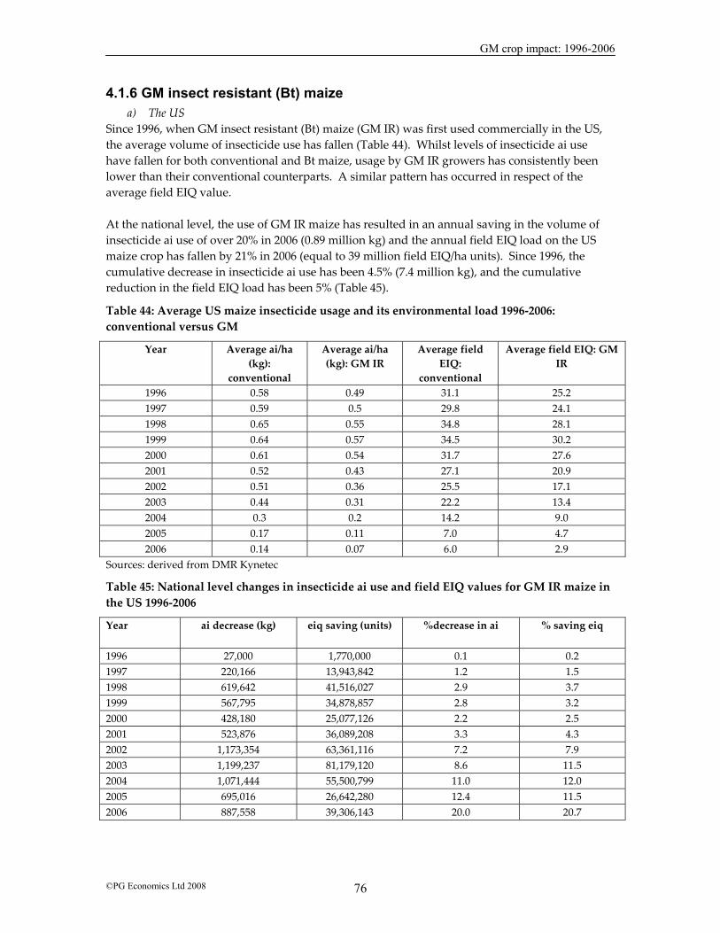
GM crop impact: 1996-2006
©PG Economics Ltd 2008 76
4.1.6 GM insect resistant (Bt) maize a) The US
Since 1996, when GM insect resistant (Bt) maize (GM IR) was first used commercially in the US, the average volume of insecticide use has fallen (Table 44). Whilst levels of insecticide ai use have fallen for both conventional and Bt maize, usage by GM IR growers has consistently been lower than their conventional counterparts. A similar pattern has occurred in respect of the average field EIQ value. At the national level, the use of GM IR maize has resulted in an annual saving in the volume of insecticide ai use of over 20% in 2006 (0.89 million kg) and the annual field EIQ load on the US maize crop has fallen by 21% in 2006 (equal to 39 million field EIQ/ha units). Since 1996, the cumulative decrease in insecticide ai use has been 4.5% (7.4 million kg), and the cumulative reduction in the field EIQ load has been 5% (Table 45).
Table 44: Average US maize insecticide usage and its environmental load 1996-2006: conventional versus GM
Year Average ai/ha (kg):
conventional
Average ai/ha (kg): GM IR
Average field EIQ:
conventional
Average field EIQ: GM IR
1996 0.58 0.49 31.1 25.2 1997 0.59 0.5 29.8 24.1 1998 0.65 0.55 34.8 28.1 1999 0.64 0.57 34.5 30.2 2000 0.61 0.54 31.7 27.6 2001 0.52 0.43 27.1 20.9 2002 0.51 0.36 25.5 17.1 2003 0.44 0.31 22.2 13.4 2004 0.3 0.2 14.2 9.0 2005 0.17 0.11 7.0 4.7 2006 0.14 0.07 6.0 2.9
Sources: derived from DMR Kynetec
Table 45: National level changes in insecticide ai use and field EIQ values for GM IR maize in the US 1996-2006
Year ai decrease (kg)
eiq saving (units) %decrease in ai % saving eiq
1996 27,000 1,770,000 0.1 0.2 1997 220,166 13,943,842 1.2 1.5 1998 619,642 41,516,027 2.9 3.7 1999 567,795 34,878,857 2.8 3.2 2000 428,180 25,077,126 2.2 2.5 2001 523,876 36,089,208 3.3 4.3 2002 1,173,354 63,361,116 7.2 7.9 2003 1,199,237 81,179,120 8.6 11.5 2004 1,071,444 55,500,799 11.0 12.0 2005 695,016 26,642,280 12.4 11.5 2006 887,558 39,306,143 20.0 20.7

GM crop impact: 1996-2006
©PG Economics Ltd 2008 77
This analysis probably understates the positive environmental impact of the technology because it understates the average values for insecticide ai/ha use and field EIQ/ha of conventional producers as the level of GM IR maize usage increases. This is because the first users of the technology tend to be those with greatest and most frequent incidence of corn boring pest and corn rootworm infestations and hence have been the greatest users of insecticides. Once uptake of the technology began to account for more than 10%-20% of total production (from 1998), the residual conventional maize growers have been those in lower infestation regions, who have probably rarely, if at all used insecticide treatments targeted at corn boring pests. Accordingly, the average ai/ha and EIQ/ha values recorded for all remaining conventional maize growers tends to fall and be lower than the average would have been if all growers had still been using conventional technology. One way of addressing this deficiency is to make comparisons between a typical insecticide treatment regime for GM IR and conventional maize growers in regions with average corn boring pest infestation levels and to use the average values for insecticide use in the 1996-1998 period as the baseline for measuring the changes post adoption. This is the methodology used by Gianessi and Carpenter (1999). Applying this approach, the impact of using GM IR maize has been to reduce the average volume of insecticides used by about 0.45 kg/ha and to reduce the average field EIQ by just over 21/ha. At the national level72, this equates to 23% and 21% savings respectively in insecticide ai use and the field EIQ value for 2006. Cumulatively since 1996, the savings using this methodology have been 21.1% for insecticide ai use (14.2 million kg) and 20.1% (671 million field EIQ units)73.
b) Canada As in the US, the main impact has been associated with reduced use of insecticides. Based on analysis of a typical insecticide treatment regime targeted at corn boring pests prior to the introduction of GM IR technology that is now no longer required74, this has resulted in a farm level saving of 0.43 kg/ha of ai use and a reduction of the field EIQ/ha of 20.7/ha. Applying this saving to the area devoted to GM IR maize in 1997 and then to a maximum of 5% of the total Canadian maize area in any subsequent year, the cumulative reduction in insecticide ai use has been 248,650 kg (-65%). In terms of environmental load, the total EIQ/ha load has fallen by 12.1 million units (-60%)75.
c) Spain Based on data for early years of GM IR trait adoption when the areas planted with this trait were fairly low (1999-2001 – drawing on analysis in Brookes (2002)), the adoption of GM IR maize, has resulted in a net decrease in both the volume of insecticide used and the field EIQ/ha load76. More specifically:
72 The maximum area that the benefit could apply to was also constrained to 10% of the total US maize crop – the estimated pre-GM IR area that had traditionally received insecticide treatments targeted at corn boring pests 73 The reader should note that the absolute values cited here are not directly comparable with the values derived above because of the different baselines used. The above methodology uses the current value for conventional insecticide use (ai and field EIQ) in each year whilst the latter methodology uses the 1996-98 average values as the baseline 74 And limiting the national impact to about 5% of the total maize crop in Canada – the estimated maximum area that probably received insecticide treatments targeted at corn boring pests before the introduction of GM IR maize 75 It has not been possible to place this in context with total insecticide use on the Canadian maize crop. If however it is assumed that total insecticide use on maize/ha in Canada has been similar to usage patterns in the US, the total annual savings in insecticide ai use and EIQ load since 1999 (the first year when the area planted to GM IR maize was greater than the previous area receiving insecticide treatments targeting corn boring pests) have been 70% and 65% respectively 76 The average volume of insecticide ai used is 0.96 kg/ha and the average field EIQ is 42/ha
GM crop impact: 1996-2006
©PG Economics Ltd 2008 78
• The volume of insecticide ai use77 was 58% lower than the level would probably have been if the crop had been all non GM in 2005 (-51,600 kg). Since 1998 the cumulative saving (relative to the level of use if all of the crop had been non GM) was 291,920 kg of insecticide ai (a 37% decrease);
• The field EIQ/ha load has fallen by 33% since 1999 (-12.7 million units). In 2006, the field EIQ load was 52% lower than its conventional equivalent.
d) Argentina
Although, GM IR maize has been grown commercially in Argentina since 1998, the environmental impact of the technology has been very small. This is because insecticides have not traditionally been used on maize in Argentina (the average expenditure on all insecticides has only been $1-$2/ha), and very few farmers have used insecticides targeted at corn boring pests. This absence of conventional treatments reflects several reasons including poor efficacy of the insecticides, the need to get spray timing right (at time of corn borer hatching), seasonal and annual variations in pest pressure and lack of awareness as to the full level of yield damage inflicted by the pest. As indicated in section 3, the main benefits from using the technology have been significantly higher levels of average yield, reduced production risk and improved quality of grain.
e) South Africa Due to the limited availability of insecticide usage data in South Africa, the estimates of the impact on insecticide use from use of GM IR maize in South Africa presented below are based on the following assumptions:
• Irrigated crops are assumed to use two applications of cypermethrin to control corn boring pests. This equates to about 0.168 kg/ha of active ingredient and a field EIQ of 4.59/ha (applicable to area of 200,000 ha);
• A dryland crop area of about 1,768,000 ha is assumed to receive an average of one application of cypermethrin. This amounts to 0.084 kg/ha of active ingredient and has a field EIQ of 2.29/ha;
• The first 200,000 ha to adopt GM IR technology is assumed to be irrigated crops. Based on these assumptions:
• In 2006, the adoption of GM IR maize resulted in a net reduction in the volume of insecticides used of almost 100,000 kg (relative to the volume that would probably have been used if 1.968 million ha had been treated with insecticides targeted at corn boring pests). The EIQ load was 60% lower than it would otherwise have been in the absence of use of the GM IR technology);
• Cumulatively since 2000, the reductions in the volume of ai use and the associated environmental load from sprayed insecticides were both 26% (-300,000 kg ai).
f) Other countries
GM IR maize has also been grown on significant areas in the Philippines (since 2003: 104,000 ha planted in 2006) and in Uruguay (since 2004: 35,000 ha in 2006). Due to limited availability on
77 Insecticides that target corn boring pests
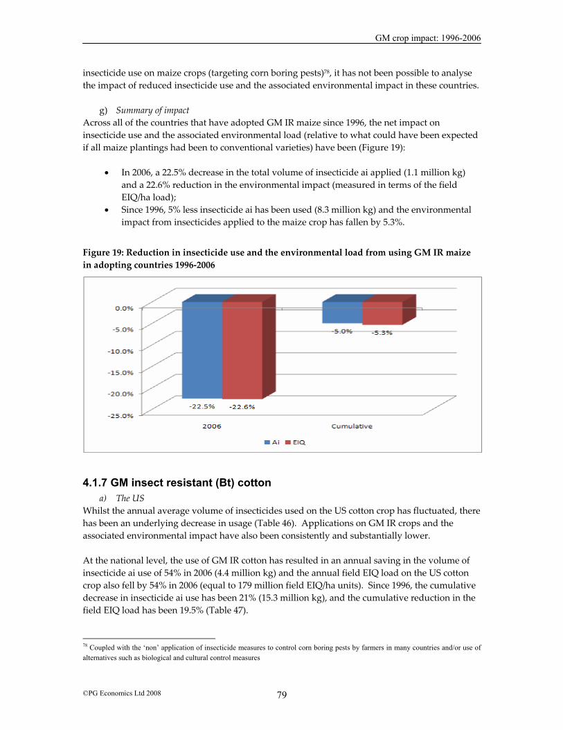
GM crop impact: 1996-2006
©PG Economics Ltd 2008 79
insecticide use on maize crops (targeting corn boring pests)78, it has not been possible to analyse the impact of reduced insecticide use and the associated environmental impact in these countries.
g) Summary of impact Across all of the countries that have adopted GM IR maize since 1996, the net impact on insecticide use and the associated environmental load (relative to what could have been expected if all maize plantings had been to conventional varieties) have been (Figure 19):
• In 2006, a 22.5% decrease in the total volume of insecticide ai applied (1.1 million kg) and a 22.6% reduction in the environmental impact (measured in terms of the field EIQ/ha load);
• Since 1996, 5% less insecticide ai has been used (8.3 million kg) and the environmental impact from insecticides applied to the maize crop has fallen by 5.3%.
Figure 19: Reduction in insecticide use and the environmental load from using GM IR maize in adopting countries 1996-2006
4.1.7 GM insect resistant (Bt) cotton a) The US
Whilst the annual average volume of insecticides used on the US cotton crop has fluctuated, there has been an underlying decrease in usage (Table 46). Applications on GM IR crops and the associated environmental impact have also been consistently and substantially lower. At the national level, the use of GM IR cotton has resulted in an annual saving in the volume of insecticide ai use of 54% in 2006 (4.4 million kg) and the annual field EIQ load on the US cotton crop also fell by 54% in 2006 (equal to 179 million field EIQ/ha units). Since 1996, the cumulative decrease in insecticide ai use has been 21% (15.3 million kg), and the cumulative reduction in the field EIQ load has been 19.5% (Table 47).
78 Coupled with the ‘non’ application of insecticide measures to control corn boring pests by farmers in many countries and/or use of alternatives such as biological and cultural control measures
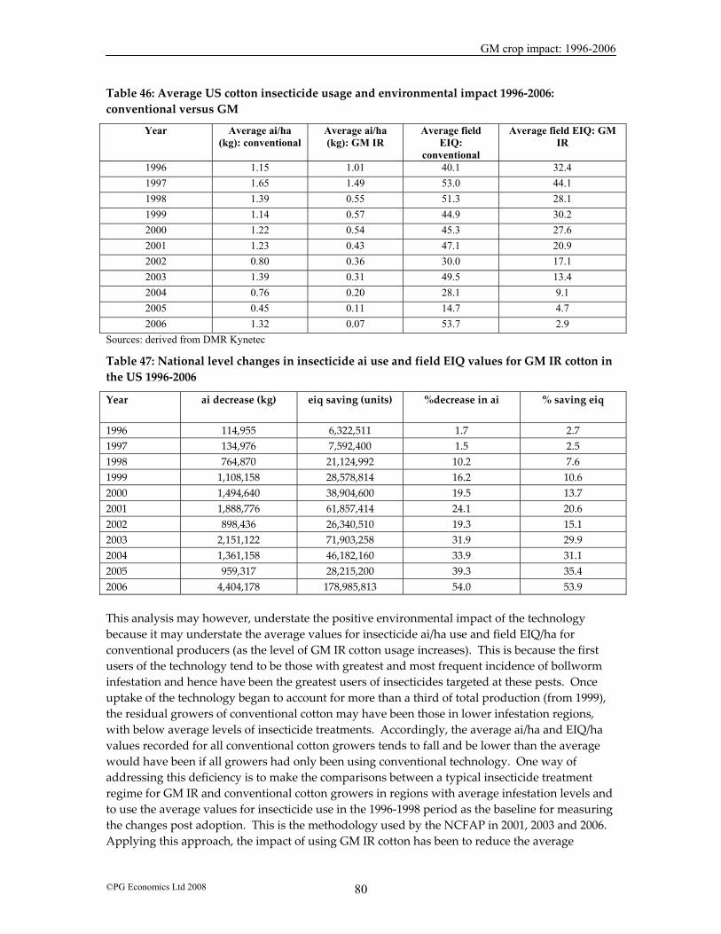
GM crop impact: 1996-2006
©PG Economics Ltd 2008 80
Table 46: Average US cotton insecticide usage and environmental impact 1996-2006: conventional versus GM
Year Average ai/ha (kg): conventional
Average ai/ha (kg): GM IR
Average field EIQ:
conventional
Average field EIQ: GM IR
1996 1.15 1.01 40.1 32.4 1997 1.65 1.49 53.0 44.1 1998 1.39 0.55 51.3 28.1 1999 1.14 0.57 44.9 30.2 2000 1.22 0.54 45.3 27.6 2001 1.23 0.43 47.1 20.9 2002 0.80 0.36 30.0 17.1 2003 1.39 0.31 49.5 13.4 2004 0.76 0.20 28.1 9.1 2005 0.45 0.11 14.7 4.7 2006 1.32 0.07 53.7 2.9
Sources: derived from DMR Kynetec
Table 47: National level changes in insecticide ai use and field EIQ values for GM IR cotton in the US 1996-2006
Year ai decrease (kg)
eiq saving (units) %decrease in ai % saving eiq
1996 114,955 6,322,511 1.7 2.7 1997 134,976 7,592,400 1.5 2.5 1998 764,870 21,124,992 10.2 7.6 1999 1,108,158 28,578,814 16.2 10.6 2000 1,494,640 38,904,600 19.5 13.7 2001 1,888,776 61,857,414 24.1 20.6 2002 898,436 26,340,510 19.3 15.1 2003 2,151,122 71,903,258 31.9 29.9 2004 1,361,158 46,182,160 33.9 31.1 2005 959,317 28,215,200 39.3 35.4 2006 4,404,178 178,985,813 54.0 53.9 This analysis may however, understate the positive environmental impact of the technology because it may understate the average values for insecticide ai/ha use and field EIQ/ha for conventional producers (as the level of GM IR cotton usage increases). This is because the first users of the technology tend to be those with greatest and most frequent incidence of bollworm infestation and hence have been the greatest users of insecticides targeted at these pests. Once uptake of the technology began to account for more than a third of total production (from 1999), the residual growers of conventional cotton may have been those in lower infestation regions, with below average levels of insecticide treatments. Accordingly, the average ai/ha and EIQ/ha values recorded for all conventional cotton growers tends to fall and be lower than the average would have been if all growers had only been using conventional technology. One way of addressing this deficiency is to make the comparisons between a typical insecticide treatment regime for GM IR and conventional cotton growers in regions with average infestation levels and to use the average values for insecticide use in the 1996-1998 period as the baseline for measuring the changes post adoption. This is the methodology used by the NCFAP in 2001, 2003 and 2006. Applying this approach, the impact of using GM IR cotton has been to reduce the average

GM crop impact: 1996-2006
©PG Economics Ltd 2008 81
volume of insecticides used by 0.28 kg/ha and to reduce the average field EIQ by 34.4/ha. At the national level, this equates to 11% and 41% savings respectively in insecticide ai use and the field EIQ value in 2006. Cumulatively since 1996, the savings using this methodology have been 7% for insecticide ai use (6.13 million kg) and 25% (753 million field EIQ units)79.
b) China Since the adoption of GM IR cotton in China there have been substantial reductions in the use of insecticides. In terms of the average volume of insecticide ai applied to cotton, the application to a typical hectare of GM IR cotton is about 1.35 kg/ha compared to 6.02 kg/ha for conventionally grown cotton (a 77% decrease: see Appendix 3)80. In terms of an average field EIQ load/ha the GM IR cotton insecticide load is 61/ha compared to 292/ha for conventional cotton. Based on these differences the amount of insecticide ai used and its environmental load impact has been 51% lower in 2006 (Table 48) than the levels that would have occurred if only non GM cotton had been planted. Cumulatively since 1997, the volume of insecticide use has decreased by 32.7% (93 million kg ai) and the field EIQ load has fallen by 33.3% (4.58 billion field EIQ/ha units).
Table 48: National level changes in insecticide ai use and field EIQ values for GM IR cotton in China 1997-2006
Year ai decrease (kg)
eiq saving (units) %decrease in ai % saving eiq
1997 158,780 7,843,630 1 1 1998 1,218,870 60,211,395 4 5 1999 3,054,180 150,874,530 14 14 2000 5,678,720 280,525,120 25 25 2001 10,152,580 501,530,930 35 36 2002 9,807,000 484,459,500 39 40 2003 13,076,000 645,946,000 42 43 2004 17,279,000 853,571,500 50 51 2005 15,411,000 761,293,500 50 51 2006 16,868,000 833,270,340 50 51
c) Australia Using a combination of data from industry sources and CSIRO81, the following changes in insecticide use on Australian cotton have occurred:
• There has been a significant reduction in both the volume of insecticides used and the environmental impact associated with this spraying (Table 49).
• The average field EIQ/ha value of the single Bt gene Ingard technology was less than half the average field EIQ/ha for conventional cotton. In turn, this saving has been further
79 The reader should note that the absolute values cited here are not directly comparable with the values derived above because of the different baselines used. The above methodology uses the current value for conventional insecticide use (ai and field EIQ) in each year whilst the latter methodology uses the 1996-98 average values as the baseline 80 Sources: based on a combination of industry views and Prey et al (2001) 81 The former making a direct comparison of insecticide use of Bollgard II versus conventional cotton and the latter a survey-based assessment of actual insecticide usage in the years 2002-03 and 2003-04

GM crop impact: 1996-2006
©PG Economics Ltd 2008 82
increased with the availability and adoption of the two Bt gene technology in Bollgard II cotton from 2003/04;
• The total amount of insecticide ai used and its environmental impact (Table 50) has been respectively 63% (1.65 million kg) and 65% lower in 2006, than the levels that would have occurred if only conventional cotton had been planted;
• Cumulatively, since 1996 the volume of insecticide use is 24.2% lower (10.3 million kg) than the amount that would have been used if GM IR technology had not been adopted and the field EIQ load has fallen by 23.6%.
Table 49: Comparison of insecticide ai use and field EIQ values for conventional, Ingard and Bollgard II cotton in Australia
Conventional Ingard Bollgard II Active ingredient use (kg/ha)
11.0 4.3 2.2
Field EIQ value/ha 220 97 39 Sources and notes: derived from Industry sources and CSIRO 2005. Ingard cotton grown from 1996, Bollgard from 2003/04
Table 50: National level changes in insecticide ai use and field EIQ values for GM IR cotton in Australia 1996-2006
Year ai decrease (kg)
eiq saving (units) %decrease in ai % saving eiq
1996 266,945 4,900,628 6.1 5.6 1997 390,175 7,162,905 9.1 8.4 1998 667,052 12,245,880 12.2 11.2 1999 896,795 16,463,550 15.2 14.0 2000 1,105,500 20,295,000 19.6 18.0 2001 909,538 16,697,496 23.8 21.9 2002 481,911 8,847,021 19.1 17.6 2003 427,621 7,850,352 20.1 18.4 2004 1,932,876 39,755,745 58.3 60.0 2005 2,177,393 44,785,011 64.4 66.2 2006 1,037,850 21,346,688 62.9 64.7
d) Argentina Adoption of GM IR cotton in Argentina has also resulted in important reductions in insecticide use82:
• The average volume of insecticide ai used by GM IR users is 44% lower than the average of 1.15 kg/ha for conventional cotton growers;
• The average field EIQ/ha is also significantly lower for GM IR cotton growers (53/ha for conventional growers compared to 21/ha for GM IR growers);
82 Based on data from Qaim and De Janvry (2005)
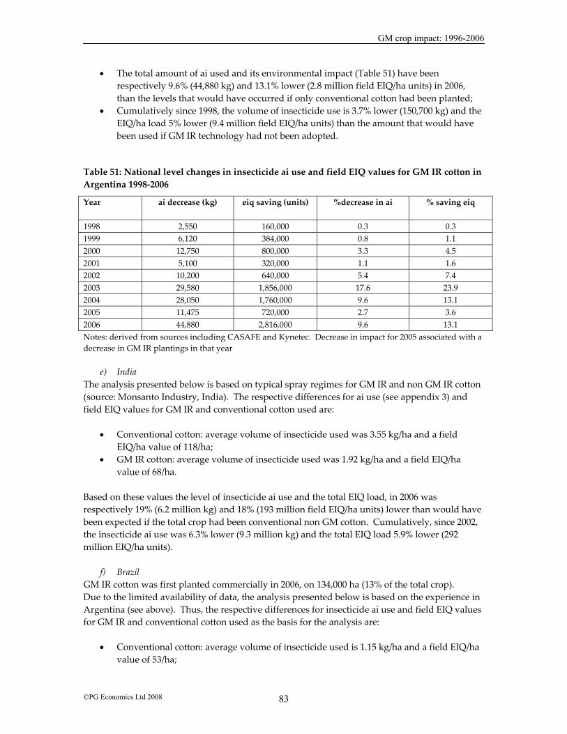
GM crop impact: 1996-2006
©PG Economics Ltd 2008 83
• The total amount of ai used and its environmental impact (Table 51) have been respectively 9.6% (44,880 kg) and 13.1% lower (2.8 million field EIQ/ha units) in 2006, than the levels that would have occurred if only conventional cotton had been planted;
• Cumulatively since 1998, the volume of insecticide use is 3.7% lower (150,700 kg) and the EIQ/ha load 5% lower (9.4 million field EIQ/ha units) than the amount that would have been used if GM IR technology had not been adopted.
Table 51: National level changes in insecticide ai use and field EIQ values for GM IR cotton in Argentina 1998-2006
Year ai decrease (kg)
eiq saving (units) %decrease in ai % saving eiq
1998 2,550 160,000 0.3 0.3 1999 6,120 384,000 0.8 1.1 2000 12,750 800,000 3.3 4.5 2001 5,100 320,000 1.1 1.6 2002 10,200 640,000 5.4 7.4 2003 29,580 1,856,000 17.6 23.9 2004 28,050 1,760,000 9.6 13.1 2005 11,475 720,000 2.7 3.6 2006 44,880 2,816,000 9.6 13.1 Notes: derived from sources including CASAFE and Kynetec. Decrease in impact for 2005 associated with a decrease in GM IR plantings in that year
e) India The analysis presented below is based on typical spray regimes for GM IR and non GM IR cotton (source: Monsanto Industry, India). The respective differences for ai use (see appendix 3) and field EIQ values for GM IR and conventional cotton used are:
• Conventional cotton: average volume of insecticide used was 3.55 kg/ha and a field EIQ/ha value of 118/ha;
• GM IR cotton: average volume of insecticide used was 1.92 kg/ha and a field EIQ/ha value of 68/ha.
Based on these values the level of insecticide ai use and the total EIQ load, in 2006 was respectively 19% (6.2 million kg) and 18% (193 million field EIQ/ha units) lower than would have been expected if the total crop had been conventional non GM cotton. Cumulatively, since 2002, the insecticide ai use was 6.3% lower (9.3 million kg) and the total EIQ load 5.9% lower (292 million EIQ/ha units).
f) Brazil GM IR cotton was first planted commercially in 2006, on 134,000 ha (13% of the total crop). Due to the limited availability of data, the analysis presented below is based on the experience in Argentina (see above). Thus, the respective differences for insecticide ai use and field EIQ values for GM IR and conventional cotton used as the basis for the analysis are:
• Conventional cotton: average volume of insecticide used is 1.15 kg/ha and a field EIQ/ha value of 53/ha;

GM crop impact: 1996-2006
©PG Economics Ltd 2008 84
• GM IR cotton: average volume of insecticide used 0.64 kg/ha and a field EIQ/ha value of 21/ha.
Based on these values the level of insecticide ai use and the total EIQ load, in 2006 were respectively 6% (68,340 kg) and 8% (4.29 million EIQ/ha units) lower than would have been expected if the total crop had been conventional cotton.
g) Mexico GM IR cotton has been grown in Mexico since 1996, and in 2006, 54,550 ha (43% of the total crop) were planted to varieties containing GM IR traits. Drawing on industry level data that compares typical insecticide treatments for GM IR and conventional cotton (see appendix 3), the main environmental impact associated with the use of GM IR technology in the cotton crop has been a significant reduction in the environmental impact associated with insecticide use on cotton. More specifically:
• On a per ha basis, GM IR cotton uses 31% less (-1.6 kg) insecticide than conventional cotton. The associated environmental impact, as measured by the EIQ indicator of the GM IR cotton is a 27% improvement on conventional cotton (a field EIQ/ha value of 74/ha compared to 259/ha for conventional cotton);
• In 2006, at a national level, there had been a 13.4% saving in the amount of insecticide active ingredient use (-88,500 kg) applied relative to usage if the whole crop had been planted to conventional varieties. The field EIQ load was 12.4% lower;
• Cumulatively since 1996, the amount of insecticide active ingredient applied was 7.2% (587,720 kg) lower relative to usage if the Mexican cotton crop had been planted to only conventional varieties over this eleven year period. The field EIQ load was 6.6% lower than it would have otherwise been if the whole crop had been using conventional varieties.
h) Other countries
Cotton farmers in South Africa and Columbia have also been using GM IR technology in recent years (respectively since 1998 and 2002). The plantings have, however been fairly small (in 2006, 9,600 ha in South Africa and 13,380 ha in Columbia). Analysis of the impact on insecticide use and the associated environmental ‘foot print’ are not presented for these crops because of the small scale and limited availability of insecticide usage data.
h) Summary of impact Since 1996, the net impact on insecticide use and the associated environmental ‘foot print’ (relative to what could have been expected if all cotton plantings had been to conventional varieties) in the main GM IR adopting countries has been (Figure 20):
• In 2006, a 37% decrease in the total volume of insecticide ai applied (28.7 million kg) and a 38.8% reduction in the environmental impact (measured in terms of the field EIQ/ha load);
• Since 1996, 22.9% less insecticide ai has been used (128 million kg) and the environmental impact from insecticides applied to the cotton crop has fallen by 24.6%.

GM crop impact: 1996-2006
©PG Economics Ltd 2008 85
Figure 20: Reduction in insecticide use and the environmental load from using GM IR cotton in adopting countries 1996-2006
4.1.8 Other environmental impacts - possible development of herbicide resistant weeds and weed shifts These possible environmental impacts associated with the adoption of GM herbicide tolerant technology have been raised in some literature and quarters. This section briefly examines the issues and evidence. The development of weeds resistant to herbicides, or of gene flow from crops to wild relatives, are not new developments in agriculture and are, therefore not issues unique to the adoption of GM technology in agriculture. All weeds have the ability to adapt to selection pressure, and there are examples of weeds that have developed resistance to a number of herbicides and to mechanical methods of weed control (eg, prostrate weeds such as dandelion which can survive mowing). Weed resistance occurs mostly when the same herbicide (s), with the same mode of action have been applied on a continuous basis over a number of years. There are hundreds of resistant weed species confirmed in the International Survey of Herbicide Resistant Weeds (www.weedscience.org). Worldwide, there are 13 weed species that are currently resistant to glyphosate, compared to over 90 weed species resistant to ALS herbicides and over 60 weed species resistant to triazine herbicides, such as atrazine. Several of the confirmed glyphosate resistant weed species have been found in areas where no GM HT crops have been grown. Prior to the commercial planting of GM HT crops, glyphosate was used before planting to control weeds. With the adoption of GM HT technology farmers were able to use glyphosate in the crop
GM crop impact: 1996-2006
©PG Economics Ltd 2008 86
to control a different set of weeds (to those in the pre-planting phase). As glyphosate is the primary herbicide used in GM HT crops planted globally, and the adoption of this technology has played a major role in facilitating the adoption of no and reduced tillage production techniques in North and South America (see section 4.2), it is possible that these factors are contributing to/could lead to the emergence of weeds resistant to herbicides like glyphosate and to weed shifts towards those weed species that are not well controlled by glyphosate. In addition, it is possible that herbicide tolerant plants could become volunteers in a subsequent crop which cannot be controlled by using glyphosate and/or there could be gene flow from the GMHT crop to wild relatives. This potential for out crossing of herbicide resistant plants with non transgenic seeds is reported to be more likely in crops such as canola and possibly sugar beet than other crops for which GM HT traits have/might be developed. Control of glyphosate resistant weeds is achieved in the same way as control of other herbicide resistant weeds, via the use of other herbicides in mixtures or sequences. GM HT crops have no effect per se on weed control as it is the herbicide programme used with them that provides the selection pressure. At the farm level, the practical consequences of glyphosate resistant weed biotypes being found are similar to the consequences of finding weeds resistant to other herbicides, namely the need to use an additional herbicide to control the resistant weed, the associated cost of this additional herbicide, and reduced management flexibility. To date, where GM HT farmers have been faced with the existence of weed species showing resistance to glyphosate these have been managed as part of a general weed control and resistance management strategy, essentially via the use of other herbicides in mixtures or sequence with glyphosate. Control of volunteer herbicide resistant crops has also been addressed in the same way, and few differences have been reported between volunteer management strategies in conventional crops compared to GM HT crops (see for example, Canola Council (2005) relating to volunteer canola management). Clearly dealing with weed resistance adds cost to farmers. Where this has occurred it has tended to reduce, marginally, the average level of cost saving and profit gains cited in the most recent studies of GM herbicide tolerant crops (and used as the basis for the analysis in section 3). Equally, from an environmental perspective, the addition of, for example a small amount of a herbicide active ingredient such as cloransulam methyl (at 0.016 kg/ha) applied pre-planting (one of the recommendations for dealing with glyphosate resistant giant ragweed in Ohio USA83), marginally worsens the environmental profile/ha relative to the original GM HT ‘recommended’ practices, but continues to be significantly better than the conventional soybean herbicide regime alternative. For example, based on the NCFAP analysis referred to in section 4.1.1, the average field EIQ/ha for GM HT soybeans in 2005 was 17.6/ha (based on using only 1.154 kg/ha of glyphosate active ingredient to control all weeds). This compares with a field EIQ/ha of 17.87/ha if 0.016kg/ha of cloransulum methyl is added to the herbicide mix to deal with glyphosate resistant giant ragweed. The average field EIQ/ha for conventional soybeans is 30.23/ha. Overall, it is important to place the possibility of negative environmental impacts associated with the use of GM HT technology occurring within the context of the current state of knowledge:
• All weeds have the ability to adapt to selection pressure;
83 Source: Ohio State University Extension Service. www.agcrops.osu.edu/soybeans
GM crop impact: 1996-2006
©PG Economics Ltd 2008 87
• The development of weed resistance (singularly or stacked) to glyphosate and problems with volunteers has not had any significant impact on the economics of using herbicide tolerant crops to date84 or on the environmental impact associated with herbicide use on GMHT crops;
• Similar problems of weed resistance build up to herbicides used on conventional arable crops have developed. The solutions are the same as in GM HT crops. Consequently, any assessment of the possible benefits and costs of GM crops should recognise this point because to only examine the possible impact of weed/pest resistance build up in relation to GM crops would not be comparing ‘like for like’ with the alternative production systems;
• New technology when introduced tends to deliver a level of benefit to farmers, who decide to adopt or, not based largely on their perception (and eventual experience) of the level of benefit for them. With time and repeated use of a specific piece of technology (eg, a particular herbicide, or seed), the effectiveness of the seed, herbicide etc declines, reducing the level of benefit derived. Eventually the technology is then replaced, itself by newer technology (eg, a new seed containing a different GM herbicide tolerant trait, or a new herbicide that may have broad spectrum applications like glyphosate, or targets the weeds that glyphosate is less effective against).
In sum, the management practice changes required to address issues such as weed resistance are relatively minor (notably rotation of herbicides and/or addition of small amounts of supplementary herbicides). The environmental impact of management changes required to facilitate this control (in terms of herbicide use and cultural practices) is also low. Hence, the environmental benefits discussed above in section 4.1 associated with changes in herbicide (and insecticide) use would only be marginally reduced in order to deal with issues of weed resistance, out crossing and weed shifts. Therefore it is likely that there would continue to be important net environmental benefits associated with the adoption of GM crops in the future.
4.2 Carbon sequestration This section assesses the contribution of GM crop adoption to reducing the level of greenhouse gas (GHG) emissions. The scope for GM crops contributing to lower levels of GHG comes from two principle sources:
• Fewer herbicide or insecticide applications (eg, targeted insecticide programmes developed in combination with GM insect resistant (IR) cotton where the number of insecticide treatments has been significantly reduced and hence there are fewer tractor spray passes);
• The use of ‘no-till’ and ‘reduced-till’85 farming systems. These have increased significantly with the adoption of GM HT crops because the GM HT technology has improved growers ability to control competing weeds, reducing the need to rely on soil cultivation and seed-bed preparation as means to getting good levels of weed control. As a result, tractor fuel use for tillage is reduced, soil quality is enhanced and levels of soil
84 See for example, Canola Council (2005) 85 No-till farming means that the ground is not ploughed at all, while reduced tillage means that the ground is disturbed less than it would be with traditional tillage systems. For example, under a no-till farming system, soybean seeds are planted through the organic material that is left over from a previous crop such as corn, cotton or wheat without any soil disturbance
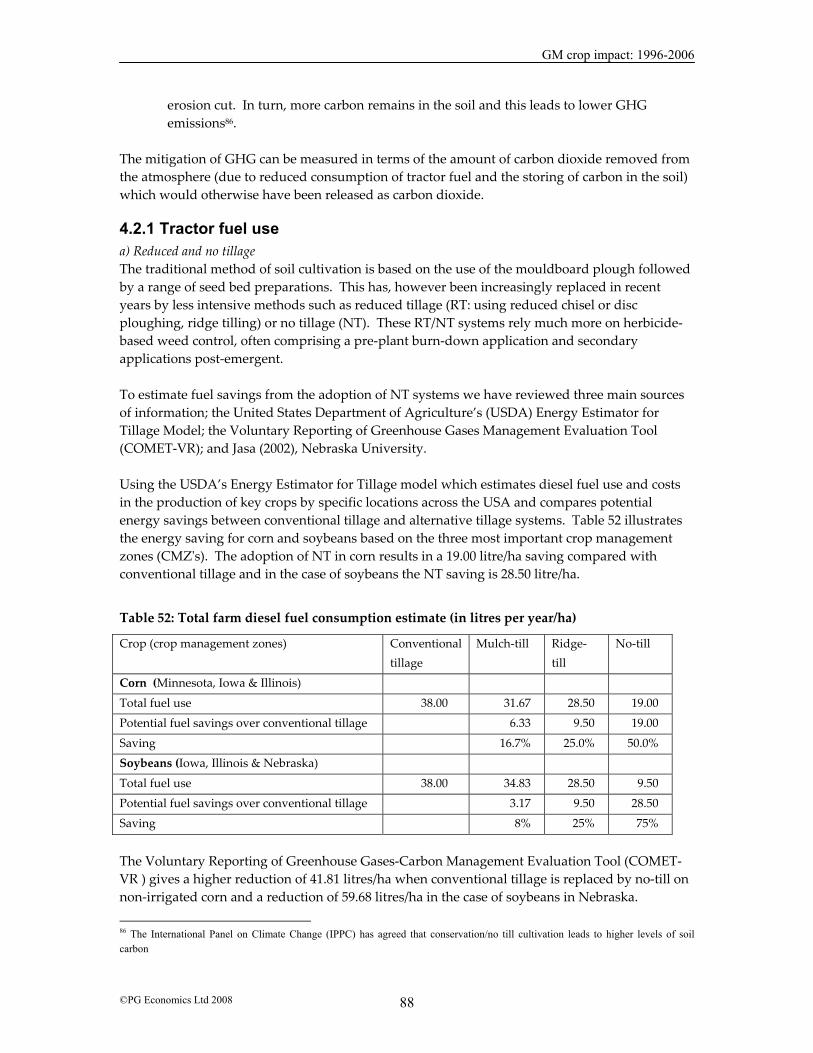
GM crop impact: 1996-2006
©PG Economics Ltd 2008 88
erosion cut. In turn, more carbon remains in the soil and this leads to lower GHG emissions86.
The mitigation of GHG can be measured in terms of the amount of carbon dioxide removed from the atmosphere (due to reduced consumption of tractor fuel and the storing of carbon in the soil) which would otherwise have been released as carbon dioxide.
4.2.1 Tractor fuel use a) Reduced and no tillage The traditional method of soil cultivation is based on the use of the mouldboard plough followed by a range of seed bed preparations. This has, however been increasingly replaced in recent years by less intensive methods such as reduced tillage (RT: using reduced chisel or disc ploughing, ridge tilling) or no tillage (NT). These RT/NT systems rely much more on herbicide-based weed control, often comprising a pre-plant burn-down application and secondary applications post-emergent. To estimate fuel savings from the adoption of NT systems we have reviewed three main sources of information; the United States Department of Agriculture’s (USDA) Energy Estimator for Tillage Model; the Voluntary Reporting of Greenhouse Gases Management Evaluation Tool (COMET-VR); and Jasa (2002), Nebraska University. Using the USDA’s Energy Estimator for Tillage model which estimates diesel fuel use and costs in the production of key crops by specific locations across the USA and compares potential energy savings between conventional tillage and alternative tillage systems. Table 52 illustrates the energy saving for corn and soybeans based on the three most important crop management zones (CMZʹs). The adoption of NT in corn results in a 19.00 litre/ha saving compared with conventional tillage and in the case of soybeans the NT saving is 28.50 litre/ha.
Table 52: Total farm diesel fuel consumption estimate (in litres per year/ha)
Crop (crop management zones) Conventional tillage
Mulch-till Ridge-till
No-till
Corn (Minnesota, Iowa & Illinois) Total fuel use 38.00 31.67 28.50 19.00 Potential fuel savings over conventional tillage 6.33 9.50 19.00
Saving 16.7% 25.0% 50.0% Soybeans (Iowa, Illinois & Nebraska) Total fuel use 38.00 34.83 28.50 9.50 Potential fuel savings over conventional tillage 3.17 9.50 28.50 Saving 8% 25% 75%
The Voluntary Reporting of Greenhouse Gases-Carbon Management Evaluation Tool (COMET-VR ) gives a higher reduction of 41.81 litres/ha when conventional tillage is replaced by no-till on non-irrigated corn and a reduction of 59.68 litres/ha in the case of soybeans in Nebraska.
86 The International Panel on Climate Change (IPPC) has agreed that conservation/no till cultivation leads to higher levels of soil carbon
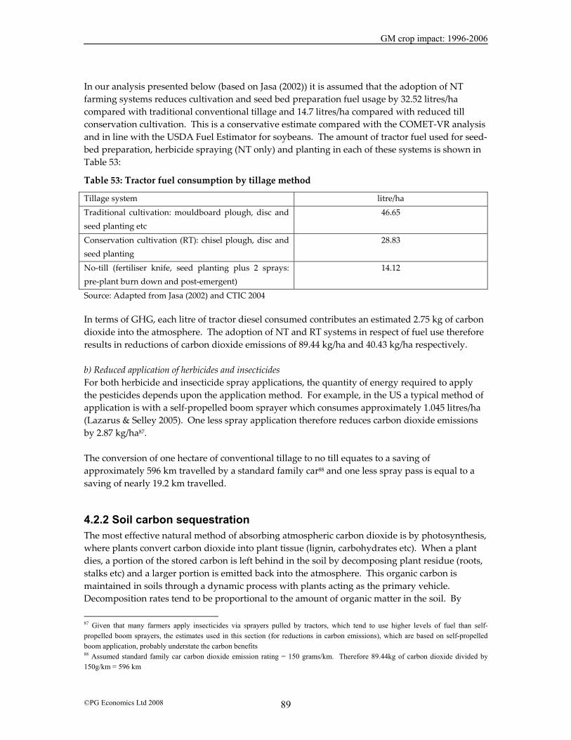
GM crop impact: 1996-2006
©PG Economics Ltd 2008 89
In our analysis presented below (based on Jasa (2002)) it is assumed that the adoption of NT farming systems reduces cultivation and seed bed preparation fuel usage by 32.52 litres/ha compared with traditional conventional tillage and 14.7 litres/ha compared with reduced till conservation cultivation. This is a conservative estimate compared with the COMET-VR analysis and in line with the USDA Fuel Estimator for soybeans. The amount of tractor fuel used for seed-bed preparation, herbicide spraying (NT only) and planting in each of these systems is shown in Table 53:
Table 53: Tractor fuel consumption by tillage method
Tillage system litre/ha Traditional cultivation: mouldboard plough, disc and seed planting etc
46.65
Conservation cultivation (RT): chisel plough, disc and seed planting
28.83
No-till (fertiliser knife, seed planting plus 2 sprays: pre-plant burn down and post-emergent)
14.12
Source: Adapted from Jasa (2002) and CTIC 2004 In terms of GHG, each litre of tractor diesel consumed contributes an estimated 2.75 kg of carbon dioxide into the atmosphere. The adoption of NT and RT systems in respect of fuel use therefore results in reductions of carbon dioxide emissions of 89.44 kg/ha and 40.43 kg/ha respectively. b) Reduced application of herbicides and insecticides For both herbicide and insecticide spray applications, the quantity of energy required to apply the pesticides depends upon the application method. For example, in the US a typical method of application is with a self-propelled boom sprayer which consumes approximately 1.045 litres/ha (Lazarus & Selley 2005). One less spray application therefore reduces carbon dioxide emissions by 2.87 kg/ha87. The conversion of one hectare of conventional tillage to no till equates to a saving of approximately 596 km travelled by a standard family car88 and one less spray pass is equal to a saving of nearly 19.2 km travelled.
4.2.2 Soil carbon sequestration The most effective natural method of absorbing atmospheric carbon dioxide is by photosynthesis, where plants convert carbon dioxide into plant tissue (lignin, carbohydrates etc). When a plant dies, a portion of the stored carbon is left behind in the soil by decomposing plant residue (roots, stalks etc) and a larger portion is emitted back into the atmosphere. This organic carbon is maintained in soils through a dynamic process with plants acting as the primary vehicle. Decomposition rates tend to be proportional to the amount of organic matter in the soil. By
87 Given that many farmers apply insecticides via sprayers pulled by tractors, which tend to use higher levels of fuel than self-propelled boom sprayers, the estimates used in this section (for reductions in carbon emissions), which are based on self-propelled boom application, probably understate the carbon benefits 88 Assumed standard family car carbon dioxide emission rating = 150 grams/km. Therefore 89.44kg of carbon dioxide divided by 150g/km = 596 km
GM crop impact: 1996-2006
©PG Economics Ltd 2008 90
enhancing the organic matter a higher Carbon-Stock Equilibrium (CSE) can be achieved. For example a shift from conventional tillage to RT/NT increases the amount of crop residue returned to the soil and decreases the decomposition rate of soil organic matter. Continuous use of NT will result in an increase in soil carbon over time until a higher CSE is reached. Changes in cultivation management can therefore potentially increase the accumulation of soil organic carbon (SOC), thereby sequestering more carbon dioxide from the atmosphere. More specifically:
• The degradation of crop soils by the oxidation of soil carbon to carbon dioxide started in the 1850’s with the introduction of large scale soil cultivation using the mouldboard plough. The effect of ploughing on soil carbon has been measured by Reicosky (1995) for a selection of cultivation techniques (after tilling wheat). Using a mouldboard plough results in soil carbon losses far exceeding the carbon value of the previous wheat crop residue and depleting soil carbon by 1,990 kg/ha compared with a no tillage system;
• Lal (1999) estimated that the global release of soil carbon since 1850 from land use changes has been 136 +/- 55 Pg89 (billion tons) of carbon. This is approximately half of the total carbon emissions from fossil fuels (270 +/- 30 Pg (billion tons)), with soil cultivation accounting for 78 +/- Pg 12 and soil erosion 26 +/- 9 Pg of carbon emissions. Lal also estimates that the potential of carbon sequestration in soil, biota and terrestrial ecosystem may be as much as 3 Pg C per year (1.41 parts per million of atmospheric carbon dioxide). A strategy of soil carbon sequestration over a 25 to 50 year period could therefore have a substantial impact on lowering the rate at which carbon dioxide is rising in the atmosphere providing the necessary time to adopt alterative energy strategies.
The contribution of a NT system as a means of sequestering soil carbon has been evaluated by West and Post (2002). This work analysed 67 long-term agricultural experiments, consisting of 276 paired treatments. These results indicate, on average, that a change from conventional tillage (CT) to no-till (NT) can sequester 57 +/- 14 g carbon per square metre per year (grams carbon m-2 year-1), excluding a change to NT in wheat-fallow systems. The cropping system that obtained the highest level of carbon sequestration when tillage changed from CT to NT was corn-soybeans in rotation (– 90 +/- 59 grams carbon m-2 year-1).) This level of carbon sequestration equates to 900 +/- 590 kg/carbon/ha/yr, which would have decreased carbon dioxide level in the atmosphere by 3,303 +/- 2,165 kg of carbon dioxide per ha/year90. More recently Johnson et al (2005) summarised how alternative tillage and cropping systems interact to sequester soil organic carbon (SOC) and impact on GHG emissions from the main agricultural area in central USA. This analysis estimated that the rate of SOC storage in NT compared to CT has been significant, but variable, averaging 400 +/- 61 kg/carbon/ha/yr (Table 54). An alternative IPCC estimate puts the rate of soil organic carbon (SOC) sequestration by the conversion from conventional to all conservation tillage (NT and RT) in North America within a range of 50 to 1,300 kg carbon/ha-1 yr-1 (it varies by soil type, cropping system and eco-region),
89 1 Pg of soil carbon pool equates to 0.47 parts per million of atmospheric carbon dioxide 90 Conversion factor for carbon sequestered into carbon dioxide = 3.67

GM crop impact: 1996-2006
©PG Economics Ltd 2008 91
with a mean of 300 kg carbon/ha-1 yr-1. Our analysis using the COMET-VR tool91 and assuming the adoption of NT from CT for non-irrigated corn in the major corn producing states results in a projected 270 to 450 kg carbon per hectare/year being sequestered (Table 54).
Table 54: Summary of the potential; of NT cultivation systems
Low kg/carbon/ha/yr
High kg/carbon/ha/yr
Average kg/carbon/ha/yr
West and Post (2002). 610 1,490 900 +/- 590 Johnson et al (2005) 339 461 400 +/- 61
Liebig (2005) 60 460 270 +/- 190 IPCC 50 1,300 300 COMET-VR (NT from CT in Corn)
Illinois 260 490 370 Minnesota 340 580 450 Nebraska 190 360 270
As well as soil cultivation other key factors influencing the rate of SOC sequestration include the amount of crop residue, soil type and soil water potential. The optimum conditions for soil sequestration are high biomass production of both surface residue and decaying roots that decompose in moist soils where aeration is not limiting. The adoption of NT systems has also had an impact on other GHG emissions. For example, methane and nitrous oxide which are respectively 21 and 310 times more potent than carbon dioxide. For example, Robertson, 2002 and Sexstone et al., 1985, suggested that the adoption of NT to sequester SOC could do so at the expense of increased nitrous oxide production where growers increase the use of nitrogen fertilizer in NT crop production systems. Robertson et al (2000) measured gas fluxes for carbon dioxide, nitrous oxide and methane and other sources of global warming potential (GWP) in cropped and unmanaged ecosystems over the period 1991 to 1999 and found that the net GWP was highest for conventional tillage systems at 114 grams of carbon dioxide equivalents per square metre/year compared with 41 grams/ha for an organic system with legumes cover and 14 grams/ha for a no-till system (with liming) and minus 20 grams/ha for a NT system (without liming). The major factors influencing the beneficial effect of no-till over conventional and organic systems is the high level of carbon sequestration and reduced use of fuel resulting in emissions of 12 grams of CO2 equivalents m-2 year-1 compared with 16 grams in conventional tillage and 19 grams for organic tillage. The release of nitrous oxide in terms of carbon dioxide was equivalent in the organic and NT systems due to the availability of nitrogen under the organic system compared with the targeted use of nitrogen fertiliser under the NT systems.
91 The Voluntary Reporting of Greenhouse Gases-Carbon Management Evaluation Tool (COMET-VR ) tool is a decision support tool for agricultural producers, land managers, soil scientists and other agricultural interests. COMET-VR provides an interface to a database containing land use data from the Carbon Sequestration Rural Appraisal (CSRA) and calculates in real time the annual carbon flux using a dynamic Century model simulation. - http://www.cometvr.colostate.edu/
GM crop impact: 1996-2006
©PG Economics Ltd 2008 92
Using IPCC emission factors, Johnson et al (2005) estimated the offsetting effect of alternative fertiliser management and cropping systems. For a NT cropping system that received 100 kg N per ha per year (net from all sources), the estimated annual nitrous oxide emission of 2.25 kg N per ha per year would have to increase by 32%-97% to completely offset carbon sequestration gains of 100-300 kg per ha per year. Estimating the full actual contribution of NT systems to soil carbon sequestration is however, made difficult by the dynamic nature of the soil sequestration process. If a specific crop area is in continuous NT crop rotation, the full SOC benefits described above can be realised. However, if the NT crop area is returned to a conventional tillage system, a proportion of the SOC gain will be lost. The temporary nature of this form of carbon storage will only become permanent when farmers adopt continuous NT systems which, itself tends to be dependant upon herbicide based weed control systems. Where the use of GM crop cultivars has resulted in a reduction in the number of spray passes or the use of less intensive cultivation practices this has provided and continues to provide for a permanent reduction in carbon dioxide emissions.
4.2.3 Herbicide tolerance and conservation tillage The adoption of GM HT crops has impacted on the type of herbicides applied, the method of application (foliar, broadcast, soil incorporated) and the number of herbicide applications. For example, the adoption of GM HT canola in North America has resulted in applications of residual soil-active herbicides being replaced by post-emergence applications of broad-spectrum herbicides with foliar activity (Brimner et al 2004). Similarly, in the case of GM HT cotton the use of glyphosate to control both grass and broadleaf weeds, post-emergent, has replaced the use of soil residual herbicides applied pre- and post emergence (McClelland et al 2000). The type and number of herbicide applications have therefore changed, often resulting in a reduction in the number of herbicide applications (see section 3). In addition to the reduction in the number of herbicide applications there has been a shift from conventional tillage to reduced/no till. This has had a marked affect on tractor fuel consumption due to energy intensive cultivation methods being replaced with no/reduced tillage and herbicide-based weed control systems. The GM HT crop where this is most evident is GM HT soybeans. Here adoption of the technology has made an important contribution to facilitating the adoption of reduced or no tillage farming92. Before the introduction of GM HT soybean cultivars, NT systems were practiced by some farmers using a number of herbicides and with varying degrees of success. The opportunity for growers to control weeds with a non residual foliar herbicide as a “burn down” pre-seeding treatment followed by a post-emergent treatment when the soybean crop became established has made the NT system more reliable, technically viable and commercially attractive. These technical advantages combined with the cost advantages have contributed to the rapid adoption of GM HT cultivars and the near doubling of the NT soybean area in the US (also more than a five fold increase in Argentina). In both countries, GM HT soybeans are estimated to account for over 95% of the NT soybean crop area.
92 See for example, CTIC 2002

GM crop impact: 1996-2006
©PG Economics Ltd 2008 93
4.2.4 Herbicide tolerant soybeans 4.2.4.1 The US Over the 1996-2006 period the area of soybeans cultivated in the USA increased by 17.6% to 30.56 million ha, 89% of which (by 2006) were GM HT cultivars. Over the same period, the area planted using conventional tillage is estimated to have fallen by 18.4% (to 5.56 million ha), whilst the area planted using reduced tillage and no-till has increased by 12.1% (to 12.5 million ha) and 56.1% (to 12.5 million ha, equal to about 40.9% of the total 2006 crop) respectively. The most rapid rate of adoption of the GM HT technology has been by growers using NT systems (GM HT cultivars accounting for an estimated 95% of total NT soybeans in 2006). This compares with conventional tillage systems for soybeans where GM HT cultivars accounting for an estimated 75% of total conventional tillage soybean plantings (Table 55).
Table 55: US soybean tillage practices and the adoption of GM HT cultivars 1996-2006 (million ha)
Total area
No till
Reduced till
Conventional till
Total GM area
Total Non GM area
No till – GM area
Reduced till GM
area
Conventional tillage GM
area
1996 26.0 8.0 11.1 6.8 0.5 25.5 0.24 0.17 0.07 1997 28.3 8.7 12.0 7.6 3.2 25.1 1.91 1.20 0.08 1998 29.1 9.4 12.8 6.9 11.8 17.4 4.81 4.45 1.97 1999 29.8 9.7 12.9 7.3 16.4 13.4 6.12 7.07 3.2 2000 30.1 10.0 12.9 7.2 18.2 11.9 7.48 8.23 3.83
2001 30.0 10.2 12.6 7.2 22.2 7.8 8.38 9.39 4.39 2002 29.5 10.3 12.3 6.9 24.3 5.3 9.31 10.49 4.46 2003 29.7 11.0 12.4 6.3 25.7 4.0 10.46 11.18 4.07 2004 30.3 11.7 12.5 6.1 27.2 3.1 11.39 11.26 4.56 2005 28.9 11.1 11.9 5.8 26.9 2.0 11.02 11.33 4.54
2006 30.6 12.5 12.5 5.6 27.2 3.4 11.88 11.25 4.17 Source: Adapted from Conservation Tillage and Plant Biotechnology (CTIC) 2002 NT = no-till + ridge till, RT = reduced tillage + mulch till, CT = conventional tillage, GM = GM HT varieties The importance of GM HT soybeans in the adoption of a NT system has also been confirmed by an American Soybean Association (ASA) study (2001) of conservation tillage. This study found that the availability of GM HT soybeans has facilitated and encouraged farmers to implement reduced tillage practices; a majority of growers surveyed indicated that GM HT soybean technology had been the factor of greatest influence in their adoption of reduced tillage practices. a) Fuel consumption Based on the soybean crop area planted by tillage system, type of seed planted (GM and non-GM) and applying the fuel usage consumption rates presented in section 4.2.193, the total consumption of tractor fuel has increased by about 43.7 million litres (from 752.7 to 796.4 million
93 Our estimates are based on the following average fuel consumption rates: NT 14.12 litre/ha, RT 28.83 litres/ha (the average of fuel consumption for chisel ploughing and disking) and conventional tillage 46.65 litres/ha
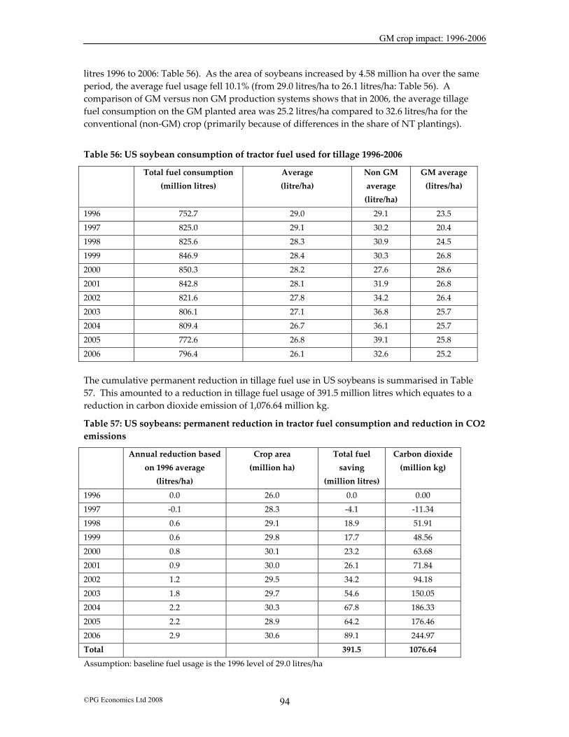
GM crop impact: 1996-2006
©PG Economics Ltd 2008 94
litres 1996 to 2006: Table 56). As the area of soybeans increased by 4.58 million ha over the same period, the average fuel usage fell 10.1% (from 29.0 litres/ha to 26.1 litres/ha: Table 56). A comparison of GM versus non GM production systems shows that in 2006, the average tillage fuel consumption on the GM planted area was 25.2 litres/ha compared to 32.6 litres/ha for the conventional (non-GM) crop (primarily because of differences in the share of NT plantings).
Table 56: US soybean consumption of tractor fuel used for tillage 1996-2006
Total fuel consumption (million litres)
Average (litre/ha)
Non GM average (litre/ha)
GM average (litres/ha)
1996 752.7 29.0 29.1 23.5 1997 825.0 29.1 30.2 20.4 1998 825.6 28.3 30.9 24.5 1999 846.9 28.4 30.3 26.8
2000 850.3 28.2 27.6 28.6 2001 842.8 28.1 31.9 26.8 2002 821.6 27.8 34.2 26.4 2003 806.1 27.1 36.8 25.7 2004 809.4 26.7 36.1 25.7 2005 772.6 26.8 39.1 25.8
2006 796.4 26.1 32.6 25.2
The cumulative permanent reduction in tillage fuel use in US soybeans is summarised in Table 57. This amounted to a reduction in tillage fuel usage of 391.5 million litres which equates to a reduction in carbon dioxide emission of 1,076.64 million kg.
Table 57: US soybeans: permanent reduction in tractor fuel consumption and reduction in CO2 emissions
Annual reduction based on 1996 average
(litres/ha)
Crop area (million ha)
Total fuel saving
(million litres)
Carbon dioxide (million kg)
1996 0.0 26.0 0.0 0.00 1997 -0.1 28.3 -4.1 -11.34 1998 0.6 29.1 18.9 51.91
1999 0.6 29.8 17.7 48.56 2000 0.8 30.1 23.2 63.68 2001 0.9 30.0 26.1 71.84 2002 1.2 29.5 34.2 94.18 2003 1.8 29.7 54.6 150.05 2004 2.2 30.3 67.8 186.33
2005 2.2 28.9 64.2 176.46 2006 2.9 30.6 89.1 244.97 Total 391.5 1076.64 Assumption: baseline fuel usage is the 1996 level of 29.0 litres/ha

GM crop impact: 1996-2006
©PG Economics Ltd 2008 95
b) Soil carbon sequestration Based on the crop area planted by tillage system and type of seed planted (GM and non-GM) and using estimates of the soil carbon sequestered by tillage system for corn and soybeans in continuous rotation (the NT system is assumed to store 300 kg of carbon/ha/year, the RT system assumed to store 100 kg carbon/ha/year and the CT system assumed to release 100 kg carbon/ha/year)94, our estimates of total soil carbon sequested are (Table 58):
• An increase of 1,607.8 million kg carbon/year (from 2,836 million kg in 1996 to 4,443.7 million kg carbon/year in 2006 due to the increase in crop area planted and the increase in the NT soybean area);
• the average level of carbon sequestered per ha increased by 36.2 kg carbon/ha/year (from 109.2 to 145.4 kg carbon/ha/year).
Table 58: US soybeans: potential soil carbon sequestration (1996 to 2006)
Total carbon sequestered (million kg) Average (kg carbon/ha)
1996 2,835.8 109.2 1997 3,045.0 107.5 1998 3,407.7 116.9 1999 3,473.3 116.4
2000 3,577.0 118.6 2001 3,600.0 120.0 2002 3,652.2 123.6 2003 3,919.9 132.0 2004 4,147.3 137.0
2005 3,950.5 136.8 2006 4,443.7 145.4
Cumulatively, since 1996 the increase in soil carbon due to the increase in RT and NT in US soybean production systems has been 4,860.1 million kg of carbon which, in terms of carbon dioxide emission equates to a saving of 17,836.58 million kg of carbon dioxide that would otherwise have been released into the atmosphere (Table 59). This estimate does not take into consideration the potential loss in carbon sequestration that might arise from a return to conventional tillage.
Table 59: US soybeans: potential additional soil carbon sequestration (1996 to 2006)
Annual increase in carbon sequestered based on 1996 average (kg carbon/ha)
Crop area (million ha)
Total carbon sequestered (million kg)
Carbon dioxide (million kg)
1996 0.0 26.0 0.0 0.00 1997 -1.7 28.3 -47.6 -174.57 1998 7.8 29.1 225.9 829.13
94 The actual rate of soil carbon sequestered by tillage system is, however dependent upon soil type, soil organic content, quantity and type of crop residue, so these estimates are indicative averages

GM crop impact: 1996-2006
©PG Economics Ltd 2008 96
1999 7.2 29.8 216.3 793.72 2000 9.5 30.1 286.1 1,050.00 2001 10.9 30.0 326.4 1,197.72
2002 14.5 29.5 427.7 1,569.57 2003 22.8 29.7 677.2 2,485.49 2004 27.8 30.3 842.5 3,092.06 2005 27.6 28.9 798.1 2,929.19 2006 36.2 30.6 1,107.4 4,064.28 Total 4,860.1 17,836.58
Assumption: carbon sequestration remains at the 1996 level of 109.2 kg carbon/ha/year 4.2.4.2Argentina Since 1996, the area planted to soybeans in Argentina has increased by 173% (from 5.9 to 16.15 million ha). Over the same period, the area planted using NT and RT practices also increased by an estimated 623%, from 2.1 to 15.2 million ha, whilst the area planted using conventional tillage decreased by 2.87 million ha, from 3.8 to 0.97 million ha: Table 60). As in the US, a key driver for the growth in NT soybean production has been the availability and rapid adoption of GM HT soybean cultivars, which in 2006 accounted for 94% of the total Argentine soybean area. As indicated in section 3, the availability of this technology has also provided an opportunity for growers to second crop soybeans in a NT system with wheat. Thus, whereas in 1996 when 6% of the total soybean crop was a second crop following on from wheat (in the same season), in 2006 the share of soybean plantings accounted for by second crop soybeans had risen to 20% of total plantings (3.2 million ha).
Table 60: Argentina soybean tillage practices and the adoption of GM cultivars 1996-2006 (million ha)
Total area No till Conventional till
Total GM area
Total non GM area
No till GM area
Conventional tillage GM
area 1996 5.9 2.1 3.8 0.04 5.88 0.04 0.00
1997 6.4 2.6 3.8 1.8 4.64 0.64 1.12 1998 7.0 3.5 3.5 4.8 2.15 2.26 2.54 1999 8.2 5.7 2.5 6.6 1.54 4.87 1.77 2000 10.6 6.9 3.7 9.0 1.59 6.56 2.44 2001 11.5 8.3 3.2 10.9 0.57 8.32 2.60 2002 13.0 9.7 3.3 12.4 0.52 9.70 2.74
2003 13.5 10.6 2.9 13.2 0.27 10.56 2.67 2004 14.3 12.6 1.8 14.1 0.29 12.57 1.49 2005 15.2 13.2 2.0 15.0 0.15 13.21 1.84 2006 16.15 15.18 0.97 15.84 0.31 15.18 0.66
Adapted from Benbrook and Trigo NT = No-till + reduced till, CT=conventional tillage a) Fuel consumption
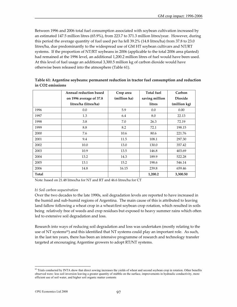
GM crop impact: 1996-2006
©PG Economics Ltd 2008 97
Between 1996 and 2006 total fuel consumption associated with soybean cultivation increased by an estimated 147.5 million litres (65.9%), from 223.7 to 371.3 million litres/year. However, during this period the average quantity of fuel used per ha fell 39.2% (14.8 litres/ha) from 37.8 to 23.0 litres/ha, due predominantly to the widespread use of GM HT soybean cultivars and NT/RT systems. If the proportion of NT/RT soybeans in 2006 (applicable to the total 2006 area planted) had remained at the 1996 level, an additional 1,200.2 million litres of fuel would have been used. At this level of fuel usage an additional 3,300.5 million kg of carbon dioxide would have otherwise been released into the atmosphere (Table 61).
Table 61: Argentine soybeans: permanent reduction in tractor fuel consumption and reduction in CO2 emissions
Annual reduction based on 1996 average of 37.8
litres/ha (litres/ha)
Crop area (million ha)
Total fuel saving million
litres
Carbon Dioxide
(million kg) 1996 0.0 5.9 0.0 0.00 1997 1.3 6.4 8.0 22.13
1998 3.8 7.0 26.3 72.19 1999 8.8 8.2 72.1 198.15 2000 7.6 10.6 80.6 221.76 2001 9.4 11.5 108.1 297.30 2002 10.0 13.0 130.0 357.42 2003 10.9 13.5 146.8 403.69
2004 13.2 14.3 189.9 522.28 2005 13.1 15.2 198.6 546.14 2006 14.8 16.15 239.8 659.46 Total 1,200.2 3,300.50
Note: based on 21.48 litres/ha for NT and RT and 46.6 litres/ha for CT b) Soil carbon sequestration Over the two decades to the late 1990s, soil degradation levels are reported to have increased in the humid and sub-humid regions of Argentina. The main cause of this is attributed to leaving land fallow following a wheat crop in a wheat:first soybean crop rotation, which resulted in soils being relatively free of weeds and crop residues but exposed to heavy summer rains which often led to extensive soil degradation and loss. Research into ways of reducing soil degradation and loss was undertaken (mostly relating to the use of NT systems95) and this identified that NT systems could play an important role. As such, in the last ten years, there has been an intensive programme of research and technology transfer targeted at encouraging Argentine growers to adopt RT/NT systems.
95 Trials conducted by INTA show that direct sowing increases the yields of wheat and second soybean crop in rotation. Other benefits observed were: less soil inversion leaving a greater quantity of stubble on the surface, improvements in hydraulic conductivity, more efficient use of soil water, and higher soil organic matter contents

GM crop impact: 1996-2006
©PG Economics Ltd 2008 98
Specific research into soil carbon sequestration in Argentina is, however limited, although Fabrizzi et al (2003) indicated that a higher level of total organic carbon was retained in the soil with NT system compared with a CT system, although no quantification was provided. Applying a conservative estimate of soil carbon retention of 100 kg/carbon/ha/yr for NT/RT soybean cropping in Argentina, a cumulative total of 9,538 million kg of carbon, which equates to a saving of 35,003 million kg of carbon dioxide has been retained in the soil that would otherwise have been released into the atmosphere (Table 62).
Table 62: Argentine soybeans: potential additional soil carbon sequestration (1996 to 2006)
Annual increase in carbon
sequestered based on 1996
average (kg carbon/ha)
Crop area (million ha)
Total carbon sequestered million
kg
Carbon dioxide (million kg)
1996 0.0 5.9 0.0 0.00 1997 10.0 6.4 63.9 234.65 1998 30.0 7.0 208.6 765.65 1999 70.0 8.2 572.6 2,101.44
2000 60.5 10.6 640.8 2,351.82 2001 74.7 11.5 859.1 3,152.99 2002 79.7 13.0 1,032.9 3,790.59 2003 86.4 13.5 1,166.6 4,281.31 2004 105.2 14.3 1,509.3 5,538.99
2005 103.8 15.2 1,578.2 5,792.04 2006 118.0 16.2 1,905.7 6,993.92 Cumulative total 9,537.7 35,003.41 Assumption: NT = +100 kg carbon/ha/yr, CT = -100 kg carbon/ha/yr Recent research by Steinbach and Alvarez (2006) on the potential of NT cropping across the Argentine Pampas indicated a potential to increase SOC by 74 Tg carbon if the whole Pampean cropping area was converted to NT. This rate of carbon sequestration is about twice the annual carbon emissions from total fossil fuels consumption in Argentina. 4.2.4.3 Paraguay and Uruguay NT/RT systems have also become important in soybean production in both Paraguay and Uruguay, where the majority of production in both countries are reported by industry sources to use NT/RT systems. a) Fuel consumption Using the findings and assumptions applied to Argentina (see above), the savings in fuel consumption for soybean production between 1996 and 2006 (associated with changes in no/reduced tillage systems, the adoption of GM HT technology and comparing the proportion of NT/RT soybeans in 2006 relative to the 1996 level) has possibly amounted to about 147 million

GM crop impact: 1996-2006
©PG Economics Ltd 2008 99
litres. At this level of fuel saving the reduction in the level of carbon dioxide release into the atmosphere has probably been lower by 404.27 million kg. b) Soil carbon sequestration Applying the same rate of soil carbon retention for NT/RT soybeans as Argentina the cumulative increase in soil carbon since 1996, due to the increase in NT/RT in Paraguay and Uruguay soybean production systems may have been 947 million kg of carbon. In terms of carbon dioxide emission this equates to a saving of 3,473.98 million kg of carbon dioxide that may otherwise have been released into the atmosphere.
4.2.5 Herbicide tolerant canola The analysis presented below relates to Canada only and does not include the US GM HT canola crop. This reflects the lack of information about the level of RT/NT in the US canola crop. Also the area devoted to GM HT canola in the US is relatively small by comparison to the corresponding area in Canada (0.42 million ha in 2006 compared to 5.08 million ha). The cumulative permanent reduction in tillage fuel use in Canadian canola since 1996 was 222.9 million litres which equates to reduction in carbon dioxide emission of 612.94 million kg (Table 63).
Table 63: Canadian canola: permanent reduction in tractor fuel consumption and reduction in CO2 emissions
Annual reduction based on 1996 average 38.5
(litres/ha)
Crop area (million ha)
Total fuel saving m litres
Carbon dioxide (million kg)
1996 0.0 3.5 0.0 0.00 1997 1.6 4.9 7.9 21.78 1998 1.6 5.4 8.8 24.28 1999 1.6 5.6 9.0 24.88
2000 1.6 4.9 7.9 21.73 2001 3.3 3.8 12.3 33.85 2002 4.9 3.3 15.9 43.76 2003 6.5 4.7 30.5 83.88 2004 8.1 4.9 40.2 110.43 2005 7.4 5.5 40.8 112.13
2006 9.8 5.1 49.5 136.22 Total 222.9 612.94 Notes: fuel usage NT = 14.12 litres/ha CT = 46.6 litres/ha In terms of the increase in soil carbon associated with the increase in RT and NT in Canadian canola production, the estimated values are summarised in Table 64. The cumulative increase in soil carbon has been 2,056 million kg of carbon which in terms of carbon dioxide emission equates to a saving of 7,545 million kg of carbon dioxide that would otherwise have been released into the atmosphere.
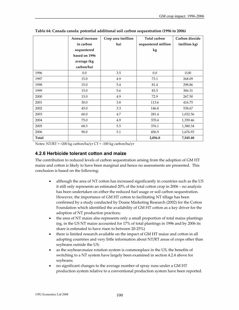
GM crop impact: 1996-2006
©PG Economics Ltd 2008 100
Table 64: Canada canola: potential additional soil carbon sequestration (1996 to 2006)
Annual increase in carbon
sequestered based on 1996
average (kg carbon/ha)
Crop area (million ha)
Total carbon sequestered million
kg
Carbon dioxide (million kg)
1996 0.0 3.5 0.0 0.00 1997 15.0 4.9 73.1 268.09
1998 15.0 5.4 81.4 298.86 1999 15.0 5.6 83.5 306.31 2000 15.0 4.9 72.9 267.50 2001 30.0 3.8 113.6 416.75 2002 45.0 3.3 146.8 538.67 2003 60.0 4.7 281.4 1,032.56
2004 75.0 4.9 370.4 1,359.46 2005 68.5 5.5 376.1 1,380.34 2006 90.0 5.1 456.9 1,676.93 Total 2,056.0 7,545.48
Notes: NT/RT = +200 kg carbon/ha/yr CT = -100 kg carbon/ha/yr
4.2.6 Herbicide tolerant cotton and maize The contribution to reduced levels of carbon sequestration arising from the adoption of GM HT maize and cotton is likely to have been marginal and hence no assessments are presented. This conclusion is based on the following:
• although the area of NT cotton has increased significantly in countries such as the US it still only represents an estimated 20% of the total cotton crop in 2006 – no analysis has been undertaken on either the reduced fuel usage or soil carbon sequestration. However, the importance of GM HT cotton to facilitating NT tillage has been confirmed by a study conducted by Doane Marketing Research (2002) for the Cotton Foundation which identified the availability of GM HT cotton as a key driver for the adoption of NT production practices;
• the area of NT maize also represents only a small proportion of total maize plantings (eg, in the US NT maize accounted for 17% of total plantings in 1996 and by 2006 its share is estimated to have risen to between 20-25%)
• there is limited research available on the impact of GM HT maize and cotton in all adopting countries and very little information about NT/RT areas of crops other than soybeans outside the US;
• as the soybean:maize rotation system is commonplace in the US, the benefits of switching to a NT system have largely been examined in section 4.2.4 above for soybeans;
• no significant changes to the average number of spray runs under a GM HT production system relative to a conventional production system have been reported.
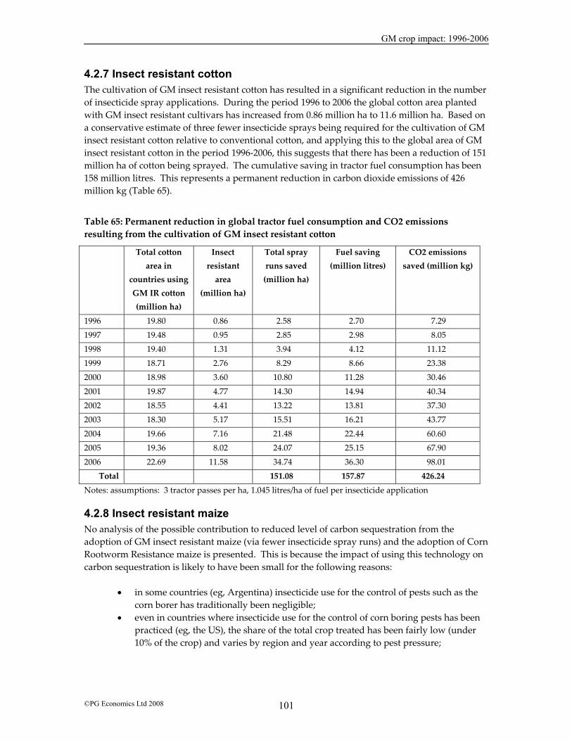
GM crop impact: 1996-2006
©PG Economics Ltd 2008 101
4.2.7 Insect resistant cotton The cultivation of GM insect resistant cotton has resulted in a significant reduction in the number of insecticide spray applications. During the period 1996 to 2006 the global cotton area planted with GM insect resistant cultivars has increased from 0.86 million ha to 11.6 million ha. Based on a conservative estimate of three fewer insecticide sprays being required for the cultivation of GM insect resistant cotton relative to conventional cotton, and applying this to the global area of GM insect resistant cotton in the period 1996-2006, this suggests that there has been a reduction of 151 million ha of cotton being sprayed. The cumulative saving in tractor fuel consumption has been 158 million litres. This represents a permanent reduction in carbon dioxide emissions of 426 million kg (Table 65).
Table 65: Permanent reduction in global tractor fuel consumption and CO2 emissions resulting from the cultivation of GM insect resistant cotton
Total cotton area in
countries using GM IR cotton (million ha)
Insect resistant
area (million ha)
Total spray runs saved
(million ha)
Fuel saving (million litres)
CO2 emissions saved (million kg)
1996 19.80 0.86 2.58 2.70 7.29 1997 19.48 0.95 2.85 2.98 8.05 1998 19.40 1.31 3.94 4.12 11.12 1999 18.71 2.76 8.29 8.66 23.38 2000 18.98 3.60 10.80 11.28 30.46
2001 19.87 4.77 14.30 14.94 40.34 2002 18.55 4.41 13.22 13.81 37.30 2003 18.30 5.17 15.51 16.21 43.77 2004 19.66 7.16 21.48 22.44 60.60 2005 19.36 8.02 24.07 25.15 67.90
2006 22.69 11.58 34.74 36.30 98.01 Total 151.08 157.87 426.24
Notes: assumptions: 3 tractor passes per ha, 1.045 litres/ha of fuel per insecticide application
4.2.8 Insect resistant maize No analysis of the possible contribution to reduced level of carbon sequestration from the adoption of GM insect resistant maize (via fewer insecticide spray runs) and the adoption of Corn Rootworm Resistance maize is presented. This is because the impact of using this technology on carbon sequestration is likely to have been small for the following reasons:
• in some countries (eg, Argentina) insecticide use for the control of pests such as the corn borer has traditionally been negligible;
• even in countries where insecticide use for the control of corn boring pests has been practiced (eg, the US), the share of the total crop treated has been fairly low (under 10% of the crop) and varies by region and year according to pest pressure;

GM crop impact: 1996-2006
©PG Economics Ltd 2008 102
• nominal application savings have occurred in relation to the adoption of GM CRW maize where over 4.0 million ha were planted in 2006. The adoption of the GM CRW may become increasing important with wider adoption of no-till cultivation systems due to the potential increase in soil-borne pests.
4.2.9 Summary of carbon sequestration impact A summary of the carbon sequestration impact is presented in Table 66. This shows the following key points:
• The permanent savings in carbon dioxide emissions (arising from reduced fuel use of 2,120 million litres of fuel) since 1996 have been about 5,821 million kg;
• The additional amount of soil carbon sequestered since 1996 has been equivalent to 63,859 million kg of carbon dioxide that has not been released into the global atmosphere96. The reader should note that these soil carbon savings are based on saving arising from the rapid adoption of NT/RT farming systems in North and South America for which the availability of GM HT technology has been cited by many farmers as an important facilitator. GM HT technology has therefore probably been an important contributor to this increase in soil carbon sequestration but is not the only factor of influence. Other influences such as the availability of relatively cheap generic glyphosate (the real price of glyphosate fell threefold between 1995 and 2000 once patent protection for the product expired) have also been important, as illustrated by the rapid adoption of RT/NT production systems in the Brazilian soybean sector, largely in the absence of the GM HT technology97. Cumulatively the amount of carbon sequestered may be higher than these estimates due to year-on-year benefits to soil quality, however equally with only an estimated 15%-25% of the crop area in continuous no-till systems it is likely that the total cumulative soil sequestration gains have been lower. It is nevertheless, not possible to estimate cumulative soil sequestration gains that take into account reversions to conventional tillage. Consequently, the estimate provided above of 63,859 million kg of carbon dioxide not released into the atmosphere should be treated with caution.
Table 66: Summary of carbon sequestration impact 1996-2006
Crop/trait/country Permanent fuel saving (million
litres)
Potentiel additional carbon dioxide saving
from fuel saving (million kg)
Potential additional carbon dioxide saving from soil
carbon sequestration (million kg)
US: GM HT soybeans 392 1,077 17,837 Argentina: GM HT soybeans
1,200 3,301 35,003
Other countries: GM HT soybeans
147 404 3,474
Canada: GM HT 223 613 7,545
96 These estimates are based on fairly conservative assumptions and therefore the true values could be higher. Also, some of the additional soil carbon sequestration gains from RT/NT systems may be lost if subsequent ploughing of the land occurs. Estimating the possible losses that may arise from subsequent ploughing would be complex and difficult to undertake. This factor should be taken into account when using the estimates presented in this section of the report 97 The reader should note that the estimates of soil carbon sequestration savings presented do not include any for soybeans in Brazil because we have assumed that the increase in NT/RT area has not been primarily related to the availability of GM HT technology in Brazil

GM crop impact: 1996-2006
©PG Economics Ltd 2008 103
canola Global GM IR cotton 158 426 0 Total 2,120 5,821 63,859
Notes: Other countries: GM HT soybeans Paraguay and Uruguay (applying US carbon sequestration assumptions). Brazil not included because of RT/NT adoption largely in the absence of GM HT technology Examining further the context of the carbon sequestration benefits, Table 67, measures the carbon dioxide equivalent savings associated with planting of GM crops for the latest year (2006), in terms of the number of car use equivalents. This shows that in 2006, the permanent carbon dioxide savings from reduced fuel use was the equivalent of removing nearly 0.54 million cars from the road for a year and the additional soil carbon sequestration gains were equivalent to removing nearly 6.022 million cars from the roads. In total, GM crop-related carbon dioxide emission savings in 2006 were equal to the removal from the roads of nearly 6.56 million cars, equal to about 24.7 of all registered private cars in the UK.
Table 67: Context of carbon sequestration impact 2006: car equivalents
Crop/trait/country Permanent carbon dioxide savings arising from reduced
fuel use (million kg of carbon
dioxide)
Average family car equivalents removed from the road for a year from the
permanent fuel savings
Potential additional soil
carbon sequestration
savings (million kg of carbon
dioxide)
Average family car equivalents removed from the road for a year from the
potential additional soil
carbon sequestration
US: GM HT soybeans 245 108,877 4,064 1,806,345 Argentina: GM HT soybeans
659 293,094 6,994 3,108,408
Other countries: GM HT soybeans
77 34,091 813 361,547
Canada: GM HT canola
136 60,541 1,677 745,304
Global GM IR cotton 98 43,582 0 0
Total 1,215 540,186 13,549 6,021,604 Notes: Assumption: an average family car produces 150 grams of carbon dioxide of km. A car does an average of 15,000 km/year and therefore produces 2,250 kg of carbon dioxide/year
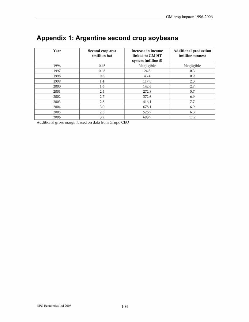
GM crop impact: 1996-2006
©PG Economics Ltd 2008 104
Appendix 1: Argentine second crop soybeans
Year Second crop area (million ha)
Increase in income linked to GM HT system (million $)
Additional production (million tonnes)
1996 0.45 Negligible Negligible 1997 0.65 24.8 0.3 1998 0.8 43.4 0.9 1999 1.4 117.8 2.3 2000 1.6 142.6 2.7 2001 2.4 272.8 5.7 2002 2.7 372.6 6.9 2003 2.8 416.1 7.7 2004 3.0 678.1 6.9 2005 2.3 526.7 6.3 2006 3.2 698.9 11.2
Additional gross margin based on data from Grupo CEO

GM crop impact: 1996-2006
©PG Economics Ltd 2008 105
Appendix 2: The Environmental Impact Quotient (EIQ): a method to measure the environmental impact of pesticides The material presented below is from the original by the cited authors of J. Kovach, C. Petzoldt, J. Degni, and J. Tette, IPM Program, Cornell University, Methods Extensive data are available on the environmental effects of specific pesticides, and the data used were gathered from a variety of sources. The Extension Toxicology Network (EXTOXNET), a collaborative education project of the environ-mental toxicology and pesticide education departments of Cornell University, Michigan State University, Oregon State University, and the University of California, was the primary source used in developing the database (Hotchkiss et al. 1989). EXTOXNET conveys pesticide-related information on the health and environmental effects of approximately 100 pesticides. A second source of information used was CHEM-NEWS of CENET, the Cornell Cooperative Extension Network. CHEM-NEWS is a computer program maintained by the Pesticide Management and Education Program of Cornell University that contains approximately 310 US EPA - Pesticide Fact Sheets, describing health, ecological, and environmental effects of the pesticides that are required for the re-registration of these pesticides (Smith and Barnard 1992). The impact of pesticides on arthropod natural enemies was determined by using the SELCTV database developed at Oregon State (Theiling and Croft 1988). These authors searched the literature and rated the effect of about 400 agrichemical pesticides on over 600 species of arthropod natural enemies, translating all pesticide/natural enemy response data to a scale ranging from one (0% effect) to five (90-100% effect). Leaching, surface loss potentials (runoff), and soil half-life data of approximately 100 compounds are contained in the National Pesticide/Soils Database developed by the USDA Agricultural Research Service and Soil Conservation Service. This database was developed from the GLEAMS computer model that simulates leaching and surface loss potential for a large number of pesticides in various soils and uses statistical methods to evaluate the interactions between pesticide properties (solubility, adsorption coefficient, and half-life) and soil properties (surface horizon thickness, organic matter content, etc.). The variables that provided the best estimate of surface loss and leaching were then selected by this model and used to classify all pesticides into risk groups (large, medium, and small) according to their potential for leaching or surface loss. Bee toxicity was determined using tables by Morse (1989) in the 1989 New York State pesticide recommendations, which contain information on the relative toxicity of pesticides to honey bees from laboratory and field tests conducted at the University of California, Riverside from 1950 to 1980. More than 260 pesticides are listed in this reference. In order to fill as many data gaps as possible, Material Safety Data Sheets (MSDS) and technical bulletins developed by the agricultural chemical industry were also used when available.

GM crop impact: 1996-2006
©PG Economics Ltd 2008 106
Health and environmental factors that addressed some of the common concerns expressed by farm workers, consumers, pest management practitioners, and other environmentalists were evaluated and are listed in Figure 1. To simplify the interpretation of the data, the toxicity of the active ingredient of each pesticide and the effect on each environmental factor evaluated were grouped into low, medium, or high toxicity categories and rated on a scale from one to five, with one having a minimal impact on the environment or of a low toxicity and five considered to be highly toxic or having a major negative effect on the environment. All pesticides were evaluated using the same criteria except for the mode of action and plant surface persistence of herbicides. As herbicides are generally systemic in nature and are not normally applied to food crops we decided to consider this class of compounds differently, so all herbicides were given a value of one for systemic activity. This has no effect on the relative rankings within herbicides, but it does make the consumer component of the equation for herbicides more realistic. Also, since plant surface persistence is only important for post-emergent herbicides and not pre-emergent herbicides, all post-emergent herbicides were assigned a value of three and pre-emergent herbicides assigned a value of one for this factor. The rating system used to develop the environmental impact quotient of pesticides (EIQ) model is as follows (l = least toxic or least harmful, 5 = most toxic or harmful):
• Mode of Action: non-systemic- 1, all herbicides – 1, systemic – 3 • Acute Dermal LD50 for Rabbits/Rats(m&/kg): >2000 – 1, 200 - 2000 – 3, 0 - 200 – 5 • Long-Term Health Effects: little or none – 1, possible- 3, definite – 5 • Plant Surface Residue Half-life: l-2 weeks- 1, 2-4 weeks- 3, > 4 weeks – 5, pre-emergent
herbicides – l, post-emergent herbicides – 3 • Soil Residue Half-life: Tl/2 <30 days – 1, Tl/2=30-100 days – 3, Tl/2 >100 days – 5 • Toxicity to Fish-96 hr LC50: > 10 ppm – 1, 1-10 ppm – 3, < 1 ppm – 5 • Toxicity to Birds-8 day LC50: > 1000 ppm – 1, 100-1000 ppm – 3, 1-100 ppm – 5 • Toxicity to Bees: relatively non toxic – 1, moderately toxic – 3, highly toxic – 5 • Toxicity to Beneficials: low impact- 1, moderate impact – 3, severe impact – 5 • Groundwater and Runoff Potential: small – 1, medium – 3, large -5
In order to further organise and simplify the data, a model was developed called the environmental impact quotient of pesticides (EIQ). This model reduces the environmental impact information to a single value. To accomplish this, an equation was developed based on the three principal components of agricultural production systems: a farm worker component, a consumer component, and an ecological component. Each component in the equation is given equal weight in the final analysis, but within each component, individual factors are weighted differently. Coefficients used in the equation to give additional weight to individual factors are also based on a one to five scale. Factors carrying the most weight are multiplied by five, medium-impact factors are multiplied by three, and those factors considered to have the least impact are multiplied by one. A consistent rule throughout the model is that the impact potential of a specific pesticide on an individual environmental factor is equal to the toxicity of the chemical times the potential for exposure. Stated simply, environmental impact is equal to toxicity times exposure. For example, fish toxicity is calculated by determining the inherent toxicity of the compound to fish times the likelihood of the fish encountering the pesticide. In this manner, compounds that are toxic to fish but short-lived have lower impact values than compounds that are toxic and long-lived.
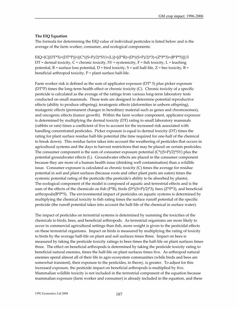
GM crop impact: 1996-2006
©PG Economics Ltd 2008 107
The EIQ Equation The formula for determining the EIQ value of individual pesticides is listed below and is the average of the farm worker, consumer, and ecological components: EIQ={C[(DT*5)+(DT*P)]+[(C*((S+P)/2)*SY)+(L)]+[(F*R)+(D*((S+P)/2)*3)+(Z*P*3)+(B*P*5)]}/3 DT = dermal toxicity, C = chronic toxicity, SY = systemicity, F = fish toxicity, L = leaching potential, R = surface loss potential, D = bird toxicity, S = soil half-life, Z = bee toxicity, B = beneficial arthropod toxicity, P = plant surface half-life. Farm worker risk is defined as the sum of applicator exposure (DT* 5) plus picker exposure (DT*P) times the long-term health effect or chronic toxicity (C). Chronic toxicity of a specific pesticide is calculated as the average of the ratings from various long-term laboratory tests conducted on small mammals. These tests are designed to determine potential reproductive effects (ability to produce offspring), teratogenic effects (deformities in unborn offspring), mutagenic effects (permanent changes in hereditary material such as genes and chromosomes), and oncogenic effects (tumor growth). Within the farm worker component, applicator exposure is determined by multiplying the dermal toxicity (DT) rating to small laboratory mammals (rabbits or rats) times a coefficient of five to account for the increased risk associated with handling concentrated pesticides. Picker exposure is equal to dermal toxicity (DT) times the rating for plant surface residue half-life potential (the time required for one-half of the chemical to break down). This residue factor takes into account the weathering of pesticides that occurs in agricultural systems and the days to harvest restrictions that may be placed on certain pesticides. The consumer component is the sum of consumer exposure potential (C*((S+P)/2)*SY) plus the potential groundwater effects (L). Groundwater effects are placed in the consumer component because they are more of a human health issue (drinking well contamination) than a wildlife issue. Consumer exposure is calculated as chronic toxicity (C) times the average for residue potential in soil and plant surfaces (because roots and other plant parts are eaten) times the systemic potential rating of the pesticide (the pesticideʹs ability to be absorbed by plants). The ecological component of the model is composed of aquatic and terrestrial effects and is the sum of the effects of the chemicals on fish (F*R), birds (D*((S+P)/2)*3), bees (Z*P*3), and beneficial arthropods(B*P*5). The environmental impact of pesticides on aquatic systems is determined by multiplying the chemical toxicity to fish rating times the surface runoff potential of the specific pesticide (the runoff potential takes into account the half-life of the chemical in surface water). The impact of pesticides on terrestrial systems is determined by summing the toxicities of the chemicals to birds, bees, and beneficial arthropods. As terrestrial organisms are more likely to occur in commercial agricultural settings than fish, more weight is given to the pesticidal effects on these terrestrial organisms. Impact on birds is measured by multiplying the rating of toxicity to birds by the average half-life on plant and soil surfaces times three. Impact on bees is measured by taking the pesticide toxicity ratings to bees times the half-life on plant surfaces times three. The effect on beneficial arthropods is determined by taking the pesticide toxicity rating to beneficial natural enemies, times the half-life on plant surfaces times five. As arthropod natural enemies spend almost all of their life in agro ecosystem communities (while birds and bees are somewhat transient), their exposure to the pesticides, in theory, is greater. To adjust for this increased exposure, the pesticide impact on beneficial arthropods is multiplied by five. Mammalian wildlife toxicity is not included in the terrestrial component of the equation because mammalian exposure (farm worker and consumer) is already included in the equation, and these
GM crop impact: 1996-2006
©PG Economics Ltd 2008 108
health effects are the results of tests conducted on small mammals such as rats, mice, rabbits, and dogs. After the data on individual factors were collected, pesticides were grouped by classes (fungicides, insecticides/miticides, and herbicides), and calculations were conducted for each pesticide. When toxicological data were missing, the average for each environmental factor within a class was determined, and this average value was substituted for the missing values. Thus, missing data did not affect the relative ranking of a pesticide within a class. The values of individual effects of each pesticide (applicator, picker, consumer, groundwater, aquatic, bird, bee, beneficials), the major components of the equation (farm worker, consumer, and ecological) and the average EIQ values are presented in separate tables (see references). EIQ field use rating Once an EIQ value has been established for the active ingredient of each pesticide, field use calculations can begin. To accurately compare pesticides and pest management strategies, the dose, the formulation or percent active ingredient of the product, and the frequency of application of each pesticide need to be determined. To account for different formulations of the same active ingredient and different use patterns, a simple equation called the EIQ field use rating was developed. This rating is calculated by multiplying the EIQ value for the specific chemical obtained in the tables by the percent active ingredient in the formulation by the rate per acre used (usually in pints or pounds of formulated product); EIQ Field Use Rating = EIQ x % active ingredient x Rate By applying the EIQ Field Use Rating, comparisons can be made between different pest management strategies or programs. To compare different pest management programs, EIQ Field Use Ratings and number of applications throughout the season are determined for each pesticide. and these values are then summed to determine the total seasonal environmental impact of the particular strategy.
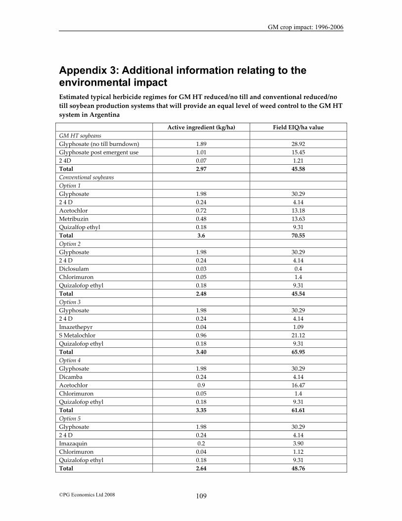
GM crop impact: 1996-2006
©PG Economics Ltd 2008 109
Appendix 3: Additional information relating to the environmental impact
Estimated typical herbicide regimes for GM HT reduced/no till and conventional reduced/no till soybean production systems that will provide an equal level of weed control to the GM HT system in Argentina
Active ingredient (kg/ha) Field EIQ/ha value GM HT soybeans Glyphosate (no till burndown) 1.89 28.92 Glyphosate post emergent use 1.01 15.45 2 4D 0.07 1.21 Total 2.97 45.58 Conventional soybeans Option 1 Glyphosate 1.98 30.29 2 4 D 0.24 4.14 Acetochlor 0.72 13.18 Metribuzin 0.48 13.63 Quizalfop ethyl 0.18 9.31 Total 3.6 70.55 Option 2 Glyphosate 1.98 30.29 2 4 D 0.24 4.14 Diclosulam 0.03 0.4 Chlorimuron 0.05 1.4 Quizalofop ethyl 0.18 9.31 Total 2.48 45.54 Option 3 Glyphosate 1.98 30.29 2 4 D 0.24 4.14 Imazethepyr 0.04 1.09 S Metalochlor 0.96 21.12 Quizalofop ethyl 0.18 9.31 Total 3.40 65.95 Option 4 Glyphosate 1.98 30.29 Dicamba 0.24 4.14 Acetochlor 0.9 16.47 Chlorimuron 0.05 1.4 Quizalofop ethyl 0.18 9.31 Total 3.35 61.61 Option 5 Glyphosate 1.98 30.29 2 4 D 0.24 4.14 Imazaquin 0.2 3.90 Chlorimuron 0.04 1.12 Quizalofop ethyl 0.18 9.31 Total 2.64 48.76
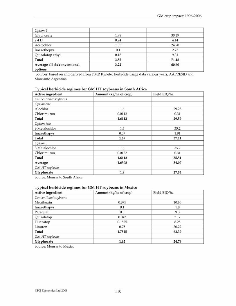
GM crop impact: 1996-2006
©PG Economics Ltd 2008 110
Option 6 Glyphosate 1.98 30.29 2 4 D 0.24 4.14 Acetochlor 1.35 24.70 Imazethepyr 0.1 2.73 Quizalofop ethyl 0.18 9.31 Total 3.85 71.18 Average all six conventional options
3.22 60.60
Sources: based on and derived from DMR Kynetec herbicide usage data various years, AAPRESID and Monsanto Argentina Typical herbicide regimes for GM HT soybeans in South Africa Active ingredient Amount (kg/ha of crop) Field EIQ/ha Conventional soybeans Option one Alochlor 1.6 29.28 Chlorimuron 0.0112 0.31 Total 1.6112 29.59 Option two S Metalochlor 1.6 35.2 Imazethapyr 0.07 1.91 Total 1.67 37.11 Option 3 S Metalochlor 1.6 35.2 Chlorimuron 0.0122 0.31 Total 1.6112 35.51 Average 1.6308 34.07 GM HT soybeans Glyphosate 1.8 27.54 Source: Monsanto South Africa Typical herbicide regimes for GM HT soybeans in Mexico Active ingredient Amount (kg/ha of crop) Field EIQ/ha Conventional soybeans Metribuzin 0.375 10.65 Imazethapyr 0.1 1.8 Paraquat 0.3 9.3 Quizalafop 0.042 2.17 Fluazafop 0.1875 8.25 Linuron 0.75 30.22 Total 1.7545 62.39 GM HT soybeans Glyphosate 1.62 24.79 Source: Monsanto Mexico
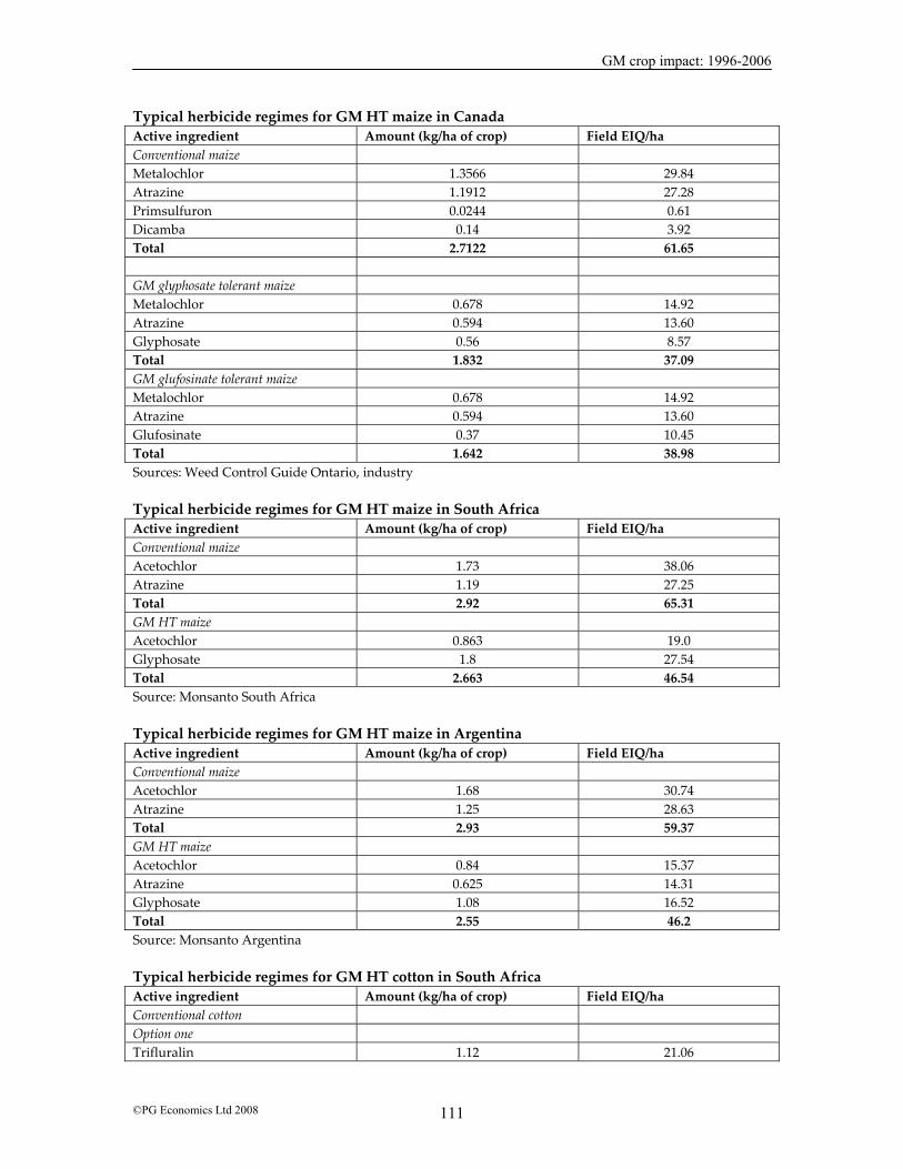
GM crop impact: 1996-2006
©PG Economics Ltd 2008 111
Typical herbicide regimes for GM HT maize in Canada Active ingredient Amount (kg/ha of crop) Field EIQ/ha Conventional maize Metalochlor 1.3566 29.84 Atrazine 1.1912 27.28 Primsulfuron 0.0244 0.61 Dicamba 0.14 3.92 Total 2.7122 61.65 GM glyphosate tolerant maize Metalochlor 0.678 14.92 Atrazine 0.594 13.60 Glyphosate 0.56 8.57 Total 1.832 37.09 GM glufosinate tolerant maize Metalochlor 0.678 14.92 Atrazine 0.594 13.60 Glufosinate 0.37 10.45 Total 1.642 38.98 Sources: Weed Control Guide Ontario, industry Typical herbicide regimes for GM HT maize in South Africa Active ingredient Amount (kg/ha of crop) Field EIQ/ha Conventional maize Acetochlor 1.73 38.06 Atrazine 1.19 27.25 Total 2.92 65.31 GM HT maize Acetochlor 0.863 19.0 Glyphosate 1.8 27.54 Total 2.663 46.54 Source: Monsanto South Africa Typical herbicide regimes for GM HT maize in Argentina Active ingredient Amount (kg/ha of crop) Field EIQ/ha Conventional maize Acetochlor 1.68 30.74 Atrazine 1.25 28.63 Total 2.93 59.37 GM HT maize Acetochlor 0.84 15.37 Atrazine 0.625 14.31 Glyphosate 1.08 16.52 Total 2.55 46.2 Source: Monsanto Argentina Typical herbicide regimes for GM HT cotton in South Africa Active ingredient Amount (kg/ha of crop) Field EIQ/ha Conventional cotton Option one Trifluralin 1.12 21.06

GM crop impact: 1996-2006
©PG Economics Ltd 2008 112
Hand weeding 0 0 Total 1.12 21.06 Option two S Metalochlor 0.95 20.9 Flumeturon 0.4 8.13 Prometryn 0.5 17.0 Total 1.85 46.03 Option 3 Trifluralin 1.12 21.06 Cyanazine 0.85 16.83 Total 1.97 37.89 Option 4 Trifluralin 0.745 14.01 Flumeturon 0.4 8.13 Prometryn 0.5 17.0 Acetochlor 0.32 5.86 Atrazine 0.128 2.93 Total 2.093 47.93 Average conventional 1.758 38.23 GM HT cotton Glyphosate 1.8 27.54 Source: Monsanto South Africa Typical herbicide regimes for GM HT cotton in Argentina Active ingredient Amount (kg/ha of crop) Field EIQ/ha Conventional cotton Glyphosate 1.8 27.54 Acetochlor 0.6 10.98 Diuron 1.034 21.20 Quizalofop 0.05 2.585 Total 3.484 62.305 GM HTcotton Glyphosate 1.8 27.54 Source: Monsanto Argentina Typical herbicide regimes for canola in the US and Canada USA Active ingredient Amount (kg/ha of crop) Field EIQ/ha Conventional canola Ethafluralin 1.053 24.54 Quizalofop 0.063 3.24 Ethametsulfuron 0.016 0.45 Total 1.132 28.23 GM glyphosate tolerant canola Glyphosate 1.12 17.14 GM glufosinate tolerant canola Glufosinate 0.41 11.7 Quizalofop 0.026 1.33 Total 0.436 13.03 Based on NCFAP 2003
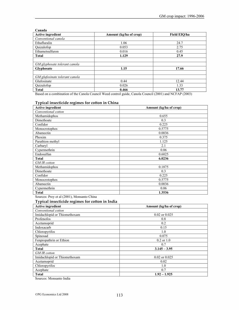
GM crop impact: 1996-2006
©PG Economics Ltd 2008 113
Canada Active ingredient Amount (kg/ha of crop) Field EIQ/ha Conventional canola Ethafluralin 1.06 24.7 Quizalofop 0.053 2.75 Ethametsulfuron 0.016 0.45 Total 1.129 27.9 GM glyphosate tolerant canola Glyphosate 1.15 17.66 GM glufosinate tolerant canola Glufosinate 0.44 12.44 Quizalofop 0.026 1.33 Total 0.466 13.77 Based on a combination of the Canola Council Weed control guide, Canola Council (2001) and NCFAP (2003) Typical insecticide regimes for cotton in China Active ingredient Amount (kg/ha of crop) Conventional cotton Methamidophos 0.655 Dimethoate 0.3 Confidor 0.225 Monocrotophos 0.5775 Abamectin 0.0036 Phoxim 0.375 Parathion methyl 1.125 Carbaryl 2.1 Cypermethrin 0.06 Endosulfan 0.6025 Total 6.0236 GM IR cotton Methamidophos 0.1875 Dimethoate 0.3 Confidor 0.225 Monocrotophos 0.5775 Abamectin 0.0036 Cypermethrin 0.06 Total 1.3536 Sources: Prey et al (2001), Monsanto China Typical insecticide regimes for cotton in India Active ingredient Amount (kg/ha of crop) Conventional cotton Imidachlopid or Thiomethoxam 0.02 or 0.025 Profenofos 0.8 Acetamoprid 0.2 Indoxacarb 0.15 Chloropyrifos 1.0 Spinosad 0.075 Fenpropathrin or Ethion 0.2 or 1.0 Acephate 0.7 Total 3.145 – 3.95 GM IR cotton Imidachlopid or Thiomethoxam 0.02 or 0.025 Acetamoprid 0.02 Chloropyrifos 1.0 Acephate 0.7 Total 1.92 – 1.925 Sources: Monsanto India

GM crop impact: 1996-2006
©PG Economics Ltd 2008 114
Typical insecticide regimes for cotton in Mexico Active ingredient Amount (kg/ha of crop) Conventional cotton Lambda cyhalothrin 0.04 Cypermethrin 0.16 Monocrotophos 0.6 Methidathion 0.622 Triazophos 0.6 Methomyl 0.225 Chlorpyrifos 0.96 Chlorfenapyr 0.12 Endosulfan 1.08 Azinphos methyl 0.315 Parathion methyl 0.5 Total 5.222 GM IR cotton Lambda cyhalothrin 0.02 Cypermethrin 0.08 Monocrotophos 0.3 Methomyl 0.225 Chlorpyrifos 0.96 Chlorfenapyr 0.12 Endosulfan 1.08 Azinphos methyl 0.315 Parathion methyl 0.5 Total 1.622 Source: Monsanto Mexico
GM crop impact: 1996-2006
©PG Economics Ltd 2008 115
References Alcade E (1999) Estimated losses from the European Corn Borer, Symposium de Sanidad Vegetal, Seveilla, Spain, cited in Brookes (2002) Alston J et al (2003) An ex-ante analysis of the benefits from adoption of corn rootworm resistant, transgenic corn technology, AgBioforum vol 5, No 3, article 1 American Soybean Association Conservation Tillage Study (2001). http://www.soygrowers.com/ctstudy/ctstudy_files/frame.htm Asia-Pacific Consortium on Agricultural Biotechnology (APCoAB) (2006) Bt cotton in India: a status report, ICRASTAT, New Delhi, India Benbrook C (2005) Rust, resistance, run down soils and rising costs – problems facing soybean producers in Argentina, Ag Biotech Infonet, paper No 8 Bennett R, Ismael Y, Kambhampati U, and Morse S (2004) Economic Impact of Genetically
Modified Cotton in India, Agbioforum Vol 7, No 3, Article 1
Brimner T A et al (2004) Influence of herbicide-resistant canola on the environmental impact of weed management. Pest Management Science Brookes G (2001) GM crop market dynamics, the case of soybeans, European Federation of Biotechnology, Briefing Paper 12 Brookes G (2002) The farm level impact of using Bt maize in Spain, ICABR conference paper 2003, Ravello, Italy. Also on www.pgeconomics.co.uk Brookes G (2005) The farm level impact of using Roundup Ready soybeans in Romania. Agbioforum Vol 8, No 4. Also available on www.pgeconomics.co.uk Brookes G (2007) The benefits of adopting GM insect resistant (Bt) maize in the EU: first results from 1998-2006. www.pgeconomics.co.uk. Also in the International Journal of Biotechnology (2008) vol 10, 2/3, pages 148-166 Brookes G, Craddock N & Kniel B (2005) The EU non GM market: labelling requirements, market dynamics and cost implications for the EU feed and food supply chains. www.eurabiobio.org, www.pgeconomics.co.uk Canola Council of Canada (2001) An agronomic & economic assessment of transgenic canola, Canola Council, Canada. www.canola-council.org Canola Council (2005) Herbicide tolerant volunteer canola management in subsequent crops, www.canolacouncil.org Carpenter J & Gianessi L (1999) Herbicide tolerant soybeans: Why growers are adopting Roundup ready varieties, Ag Bioforum, Vol 2 1999, 65-72 Carpenter J (2001) Comparing Roundup ready and conventional soybean yields 1999, National Centre for Food & Agriculture Policy, Washington Carpenter et al (2002) Comparative environmental impacts of biotech-derived and traditional soybeans, corn and cotton crops, Council for Agricultural Science and Technology (CAST), USA Carpenter J & Gianessi L (2002) Agricultural Biotechnology: updated benefit estimates, National Centre for Food and Agricultural Policy (NCFAP), Washington, USA Council for Biotechnology Information Canada (2002) Agronomic, economic and environmental impacts of the commercial cultivation of glyphosate tolerant soybeans in Ontario Conservation Tillage and Plant Biotechnology (CTIC: 2002) How new technologies can improve the environment by reducing the need to plough. http://www.ctic.purdue.edu/CTIC/Biotech.html
GM crop impact: 1996-2006
©PG Economics Ltd 2008 116
Crossan A & Kennedy I (2004) A snapshot of Roundup Ready cotton in Australia: are there environmental benefits from the rapid adoption of RR cotton, University of Sydney CSIRO (2005) The cotton consultants Australia 2005 Bollgard II comparison report, CSIRO, Australia CTIC (2007) 2006 Crop residue management survey: a survey of tillage systems usage by crop and acreas planted Doyle B et al (2003) The Performance of Roundup Ready cotton 2001-2002 in the Australian cotton sector, University of New England, Armidale, Australia Doyle B (2005) The Performance of Ingard and Bollgard II Cotton in Australia during the 2002/2003 and 2003/2004 seasons, University of New England, Armidale, Australia Fabrizzi et al (2003). Soil Carbon and Nitrogen Organic Fractions in Degraded VS Non-Degraded Mollisols in Argentina. Soil Sci. Soc. Am. J. 67:1831-1841 Fernandez-Cornejo J & Klotz-Ingram C (1998) Economic, environmental and policy impacts of using GE crops for pest management. Presented to 1998 NE Agricultural & Resource Economics Association, Itthaca, USA. Cited in Fernandez-Cornejo J & McBride W (2000) Fernandez-Cornejo J & McBride W (2000) Genetically engineered crops for pest management in US agriculture: farm level benefits, USDA, ERS Agricultural Economics Report No 786 Fernandez-Cornejo J & McBride W (2002) Adoption of bio-engineered crops, USDA, ERS Agricultural Economics Report No 810 Fernandez-Cornejo J, Heimlich R & McBride W (2000) Genetically engineered crops: has adoption reduced pesticide use, USDA Outlook August 2000 Fernandez-Cornejo J & McBride W (2000) Genetically engineered crops for pest management in US agriculture, USDA Economic Research Service report 786 Fitt G (2001) Deployment and impact of transgenic Bt cotton in Australia, reported in James C (2001), Global review of commercialised transgenic crops: 2001 feature: Bt cotton, ISAAA George Morris Centre (2004) Economic & environmental impacts of the commercial cultivation of glyphosate tolerant soybeans in Ontario, unpublished report for Monsanto Canada Gianessi L & Carpenter J (1999) Agricultural biotechnology insect control benefits, NCFAP, Washington, USA Gonsalves D (2005) Harnessing the benefits of biotechnology: the case of Bt corn in the Philippines. .ISBN 971-91904-6-9. Strive Foundation, Laguna, Philippines Gouse M et al (2006) Output & labour effect of GM maize and minimum tillage in a communal area of Kwazulu-Natal, Journal of Development Perspectives 2:2 Gouse M et al (2005) A GM subsistence crop in Africa: the case of Bt white maize in S Africa, Int Journal Biotechnology, Vol 7, No1/2/3 2005 Gouse et al (2006) Three seasons of insect resistant maize in South Africa: have small farmers benefited, AgBioforum 9 (1) 15-22 Heap I (2007) International Survey of Herbicide Resistant Weeds. Database. http://www.weedscience.org/in.asp. Huang J et al (2003) Biotechnology as a alternative to chemical pesticides: a case study of Bt cotton in China, Agricultural Economics 25, 55-67 IMRB (2006) Socio-economic benefits of Bollgard and product satisfaction (in India), IMRB International, Mumbai, India IMRB (2007) Socio-economic benefits of Bollgard and product satisfaction (in India), IMRB International, Mumbai, India Ismael Y et al (2002) A case study of smallholder farmers in the Mahathini flats, South Africa, ICABR conference, Ravello Italy 2002
GM crop impact: 1996-2006
©PG Economics Ltd 2008 117
James C (2002) Global review of commercialized transgenic crops 2001: feature Bt cotton, ISAAA No 26 James C (2006) Global status of Transgenic crops, various global review briefs from 1996 to 2006, ISAAA James C (2003) Global review of commercialized transgenic crops 2002: feature Bt maize, ISAAA No 29 James C (2006) Global status of commercialised biotech/GM crops: 2006, ISAAA brief No 35. www.isaaa.org Jasa P (2002) Conservation Tillage Systems, Extension Engineer, University of Nebraska Johnson et al (2005) Greenhouse gas contributions and mitigation potential of agriculture in the central USA. Soil Tillage Research 83 (2005) 73-94 Kirsten J et al (2002) Bt cotton in South Africa: adoption and the impact on farm incomes amongst small-scale and large-scale farmers, ICABR conference, Ravello, Italy 2002 Kleiter G et al (2005) The effect of the cultivation of GM crops on the use of pesticides and the impact thereof on the environment, RIKILT, Institute of Food Safety, Wageningen, Netherlands Kovach, J., C. Petzoldt, J. Degni and J. Tette (1992). A method to measure the environmental impact of pesticides. New Yorkʹs Food and Life Sciences Bulletin. NYS Agricul. Exp. Sta. Cornell University, Geneva, NY, 139. 8 pp. Annually updated http://www.nysipm.cornell.edu/publications/EIQ.html Lal et al (1998) The Potential for US Cropland to sequester Carbon and Mitigate the Greenhouse Effect. Ann Arbor Press, Chelsea. MI. Lal et al (1999) Managing US Crop Land to sequester carbon in soil. Journal of Soil Water Conservation, Vol 54: 374-81 Lazarus & Selley (2005) Farm Machinery Economic Cost Estimates for 2005, University of Minnesota Extension Service Leibig et al (2005) Greenhouse gas contributions and mitigation potential of agriculture practices in northwestern USA and western Canada. Soil Tillage Research 83 (2005) 25-52 Marra M, Pardey P & Alston J (2002) The pay-offs of agricultural biotechnology: an assessment of the evidence, International Food Policy Research Institute, Washington, USA Martinez-Carillo J & Diaz-Lopez N (2005) Nine years of transgenic cotton in Mexico: adoption and resistance management, Proceedings Beltwide Cotton Conference, Memphis, USA, June 2005 McClelland et al (2000) Rou, Arkansas Agricultural Experiment Station Monsanto Comercial Mexico (2005) Official report to Mexican Ministry of Agriculture, unpublished Monsanto Comercial Mexico (2007) Official report to Mexican Ministry of Agriculture of the 2006 crop, unpublished Morse S et al (2004) Why Bt cotton pays for small-scale producers in South Africa, Nature Biotechnology 22 (4) 379-380 Moschini G, Lapan H & Sobolevsky A (2000) Roundup ready soybeans and welfare effects in the soybean complex, Iowa State University, Agribusiness vol 16: 33-55 Mullins W & Hudson J (2004) Bollgard II versus Bollgard sister line economic comparisons, 2004 Beltwide cotton conferences, San Antonio, USA, Jan 2004 NCFAP (2001) Agricultural biotechnology: updated benefit estimates, Carpenter J & Gianessi L National Centre for Food & Agriculture Policy, Washington NCFAP (2003) Impacts on US agriculture of biotechnology-derived crops planted in 2003- an update of eleven case studies, Sankala S & Blumenthal E, NCFAP, Washington. www.ncfap.org NCFAP (2006) A 2006 update of impacts on US agriculture of biotechnology-derived crops planted in 2005, Sankala S, NCFAP, Washington. www.ncfap.org

GM crop impact: 1996-2006
©PG Economics Ltd 2008 118
Parana Department of Agriculture (2004) Cost of production comparison: biotech and conventional soybeans, in USDA GAIN report BR4629 of 11 November 2004. www.fas.usad.gov/gainfiles/200411/146118108.pdf PG Economics (2003) Consultancy support for the analysis of the impact of GM crops on UK farm profitability, www.pgeconomics.co.uk Pray C et al (2001) Impact of Bt cotton in China, World Development, 29(5) 1-34 Pray C et al (2002) Five years of Bt cotton in China – the benefits continue, The Plant Journal 2002, 31 (4) 423-430 Phipps R & Park J (2001) Environmental benefits of GM crops: global & European perspectives on their ability to reduce pesticide use, Journal of Animal Sciences, 11, 2002, 1-18 Qaim M & De Janvry A (2002) Bt cotton in Argentina: analysing adoption and farmers willingness to pay, American Agricultural Economics Association Annual Meeting, California, Qaim M & De Janvry A (2005) Bt cotton and pesticide use in Argentina: economic and environmental effects, Environment and Development Economics 10: 179-200 Qaim M & Traxler G (2002) Roundup Ready soybeans in Argentina: farm level, environmental and welfare effects, 6th ICABR conference, Ravello, Italy Qaim M & Traxler G (2005) Roundup Ready soybeans in Argentina: farm level & aggregate welfare effects, Agricultural Economics 32 (1) 73-86 Qaim M & Matuschke J (2006) Impact of GM crops in developing countries: a survey, Quarterly Journal of International Agriculture 44 (3) 207-227 Ramon G (2005) Acceptability survey on the 80-20 bag in a bag insect resistance management strategy for Bt corn, Biotechnology Coalition of the Philippines (BCP) Reicosky D C (1995) Conservation tillage and carbon cycling:soil as a source or sink for carbon. University of Davis Rice M (2004) Transgenic rootworm corn: assessing potential agronomic, economic and environmental benefits, Plant Health Progress 10, `094/php-2001-0301-01-RV Robertson et al (2000) Greenhouse Gases in Intensive Agriculture: Contributions of Individual Gases to the Radioactive Forces of the Atmosphere. Science Vol 289 September 15 2000 1922-1925 Runge Ford C & Ryan B (2004) The global diffusion of plant biotechnology: international adoption and research in 2004, University of Minnesota, USA Steinbach H S & Alvarez R (2006) Changes in Soil Organic Carbon Contents and Nitrous Oxide Emissions after the Introduction of No-Till in Pampean Agroecosystems. Journal Environmental Qual 35:3-13 Taylor I (2003) Cotton CRC annual report, UNE, Armidale, Cotton Research Institute, Narrabri, Australia Traxler G et al (2001) Transgenic cotton in Mexico: economic and environmental impacts, ICABR conference, Ravello, Italy Trigo et al (2002) Genetically Modified Crops in Argentina agriculture: an opened story. Libros del Zorzal, Buenos Aires, Argentina USDA (1999) Farm level effects of adopting genetically engineered crops, preliminary evidence from the US experience, Economic issues in agricultural biotechnology USDA (1999) Farm level effects of adopting genetically engineered crops, preliminary evidence from the US experience, Economic Issues in Agricultural Biotechnology West T.O. and Post W.M. (2002) Soil Organic Carbon Sequestration Rates by Tillage and Crop Rotation: A Global Analysis. Soil Science Society of American Journal. Vol 66 November/December: 930-1046 Yorobe J (2004) Economics impact of Bt corn in the Philippines. Paper presented to the 45th PAEDA Convention, Querzon City