global curvature for surfaces and area minimization under a thickness constraint

8/13/2019 Global Curvature for Surfaces and Area Minimization Under a Thickness Constraint

http://slidepdf.com/reader/full/global-curvature-for-surfaces-and-area-minimization-under-a-thickness-constraint 1/37

Calc. Var. (2006)DOI 10.1007/s00526-005-0334-9 Calculus of Variations

Paweł Strzelecki · Heiko von der Mosel

Global curvature for surfaces and areaminimization under a thickness constraint

Received: 17 November 2004 / Accepted: 16 December 2004 / Published online: 16 December 2005C Springer-Verlag 2005

Abstract Motivated by previous work on elastic rods with self-contact, involvingthe concept of the global radius of curvature for curves (as dened by Gonzalezand Maddocks), we dene the global radius of curvature [ X ] for a wide classof continuous parametric surfaces X for which the tangent plane exists on adense set of parameters. It turns out that in this class of surfaces a positive lower bound [ X ] ≥ θ > 0 provides, naively speaking, the surface with a thicknessof magnitude θ ; it serves as an excluded volume constraint for X , prevents self-intersections, and implies that the image of X is an embedded C 1-manifold with

a Lipschitz continuous normal. We also obtain a convergence and a compactnessresult for such thick surfaces, and show one possible application to variationalproblems for embedded objects: the existence of ideal surfaces of xed genus ineach isotopy class.

The proofs are based on a mixture of elementary topological, geometric andanalytic arguments, combined with a notion of the reach of a set, introduced byFederer in 1959.

Mathematics Subject Classication (2000) 49Q10, 53A05, 53C45, 57R52,74K15

P. StrzeleckiInstytut Matematyki, Uniwersytet Warszawski, ul. Banacha 2, 02–097 Warsaw, PolandE-mail: [email protected]

H. von der Mosel ( B )Institut f ur Mathematik, RWTH Aachen, Templergraben 55, 52062 Aachen, GermanyE-mail: [email protected]



P. Strzelecki, H. von der Mosel

1 Introduction

1.1 Physical and geometric motivation

Physical surfaces such as sheets of paper, thin elastic plates, pieces of cloth, or alu-minium foil often undergo large deformations in space so that different parts of thesame object touch each other. These self-contact phenomena can also be observedon various smaller length scales, especially in biological systems, e.g., pinchedskin tissue, buckled membranes, conformations of lipid vesicles under thermal in-uence [ 29]. The underlying common feature of all these examples is that of asurface with a small but positive thickness reecting the fact that interpenetrationof matter is impossible.

The mathematical modelling of the intuitively obvious mechanism of self-avoidance is a challenging task: one needs an analytically tractable notion of thick-ness for surfaces, which in particular should be accessible to variational methodsin order to deal with energy minimization problems in the framework of nonlin-ear elasticity. Moreover, surfaces with positive thickness are embedded; hence asuitable notion of self-avoidance should also lead to a novel treatment of classicalgeometric boundary value problems such as the Plateau problem or free and semi-free problems in the class of embeddings . This would produce physically relevantsolutions of xed topological type without self-intersections – in contrast to theclassical solutions, where one frequently encounters non-embedded solutions dueto the geometry of the boundary congurations, see the discussion on minimalsurfaces in [ 6, Ch. 4.10].

Our aim is to introduce and investigate a purely geometric notion of thicknessfor a large class of (nonsmooth) parametric surfaces suitable for the calculus of variations. Motivated by the second author’s previous cooperations on elastic rodswith self-contact [15, 26–28], which involved the concept of the global radius of curvature for curves as suggested by Gonzalez and Maddocks [ 14], we dene theglobal radius of curvature for surfaces . Most results of the present paper havealready been announced (without proofs) in [ 31].

1.2 Brief discussion of results

The main idea can be sketched as follows. Take a continuous parametric surface X : R 2

⊃ B 2 → R 3 (with possibly innite area) which possesses a tangent plane

on a dense subset G ⊂ B 2 which may even have zero measure. Consider the radiiof all spheres touching the surface X (B 2) in one of these points X (w),w ∈ G ,and containing at least one other point of the surface. We dene the inmum of

these radii as the global radius of curvature [ X ] of the surface X . It turns outthat a positive lower bound on [ X ] serves as an excluded volume constraint for the surface X .

In fact, one of our main results is that [ X ] ≥ θ > 0 implies that X (B 2) isa C 1,1-manifold with boundary, where the domain size and the C 1,1-norms of thelocal graph representations of X (B 2) are uniform and depend solely on the con-stant θ (Theorems 5.1 and 5.2). This result requires careful analysis of the normalin the interior and near the boundary, since the set B 2 \ G of bad points without a



Global curvature for surfaces

tangent plane is allowed to have full measure. In view of applications in the cal-

culus of variations we prove that the excluded volume constraint in terms of theglobal radius of curvature is stable under pointwise convergence of parametriza-tions, see Theorem 6.6 . Moreover, assuming a uniform upper bound on area and auniform positive lower bound on the global radius of curvature for a family of sur-faces we can prove the existence of a C 1-convergent subsequence to a limit man-ifold of class C 1,1 , again with uniform control on the local graph representations(Theorem 6.4). This compactness result may be a crucial step towards the study of variational problems for embedded surfaces in geometry and nonlinear elasticity.In fact, we show that Theorem 6.4 may be used to prove the existence of idealsurfaces of xed genus in each isotopy class, see Sect. 7. (The term ‘ideal’ is usedto describe the ‘thickest’ surface having xed area and prescribed isotopy class.)Let us also mention that our results carry over to arbitrary co-dimension and arenot restricted to disk-type surfaces.

The presentation is structured as follows: In Sect. 2 we give the precise def-initions of the class of admissible surfaces, of the global radius of curvature for surfaces and provide simple analytical and topological consequences. In Sect. 3we prove a priori estimates for the normal line depending only on a positive lower bound for the global radius of curvature. We extend these results up to the bound-ary in Sect. 4, before we study the structure of the image to prove that such asurface is a C1, 1-manifold in Sect. 5. Section 6 contains the convergence andcompactness results, which are applied in our existence proof of ideal surfacesin Sect. 7.

Before passing to the details, let us discuss some earlier papers related to our work.

1.3 Other approaches to thickness of surfaces

An alternative method to prevent a surface from self-intersecting is to introduceexplicit repulsive forces between pairs of points on the surface. Based on thisidea Kusner and Sullivan [ 18] suggested a M¨obius invariant knot energy for k -dimensional submanifolds in R n without boundary. These highly singular poten-tial energies, however, require some regularization to account for adjacent pointson the surface and, apart from the one-dimensional case of knot energies for curves[25], [11 ], [17], there are no analytical results regarding existence of minimizers or their regularity. Banavar, Gonzalez, Maddocks and Maritan [ 2] proposed so-calledmany-body potentials , replacing the Euclidean distance between two points by ge-ometric multipoint functions on curves, or tangent-point distances for surfaces asLagrangians for multiple integrals, in order to avoid the technical difculties aris-ing from the singularities in the potential, and to introduce an intrinsic length-scalefor thickness. Although not stated explicitly in [ 2] Banavar et al. clearly had theconcept of global curvature for smooth surfaces based on tangent-point distancesin mind from which their many-body potentials arise.

Apart from numerical investigations in the protein science [ 3] based on thesepotentials, however, there are, to the best of our knowledge, no analytical resultsin this direction, with one exception: For a particular example of a three-body po-tential, the so-called total Menger curvature on one-dimensional sets, there is a




impose the condition

rank DX (w) = 2 for all w ∈ G , (2.1)

so that the afne tangent plane T w X := X (w) + DX (w)( R 2) is a well-denedtwo-dimensional afne plane. In the sequel each w ∈ G ⊂ B 2 is called a good parameter , and G is referred to as the set of good parameters.

Each such mapping will be called admissible . The class of all admissible map-pings is denoted by A (B 2 , R 3). It is clear that a mapping X ∈ A (B 2 , R 3) can a priori have innite area. On the other hand, if X ∈ C1(B 2 , R 3) ∩C 0(B 2 , R 3) isan immersion, then X is contained in A (B 2 , R 3) .

Finally, note that if is an arbitrary two-dimensional Riemannian manifoldwith or without boundary then the class A ( , R 3), and in fact also A ( , R d ) ,where d ≥ 3, can be dened in a similar way.

Remark. To give an example of a well investigated class of (nonsmooth) map-pings where most of the above assumptions are automatically satised, we recallhere the denition and a handful of properties of n-absolutely continuous func-tions denoted by ACn . (In our setting n = 2.) Let ⊂ R n . One says, see Mal y[21], that f ∈ ACn ( , R d ) whenever for every ε > 0 there exists a δ > 0 suchthat for every k ∈ N and every nite family of pairwise disjoint balls B1 , . . . , Bk in the following is satised:

k

i=1

L n ( Bi ) < δ ⇒k

i=1

osc Bi

f n

< ε,

whereosc A f = sup

x , y∈

A | f ( x ) − f ( y)|stands for the oscillation of f on A and L n denotes the Lebesgue measure. Obvi-ously, such mappings are continuous. Mal y proves that n-absolute continuity (for mappings f : → R d , where d can be arbitrary) implies weak differentiabil-ity with gradient in Ln (so that for n = 2 the area of f is nite!) and classicaldifferentiability almost everywhere. Moreover, for d ≥ n the Lusin condition issatised, i.e. H n ( f ( E)) = 0 whenever L n ( E) = 0, and the area formula holds.

Thus, for planar domains , AC2( , R 3) is a proper subset of the Sobolevspace of W 1,2( , R 3) . The latter space obviously contains discontinuous map-pings; it also contains mappings which are continuous but nowhere differentiablein the classical sense. On the other hand, for every bounded domain we have

p> 2

W 1, p( , R 3) ⊂ AC2( , R 3), (2.2)

so that the class AC 2 is indeed larger than any of the Sobolev spaces W 1, p , p > 2.In fact, the inclusion in ( 2.2 ) is proper: the mapping

B 2 w −→ f (w) =w

|w |1

log (1 + |w |−1) ∈ R 2⊂

R 3




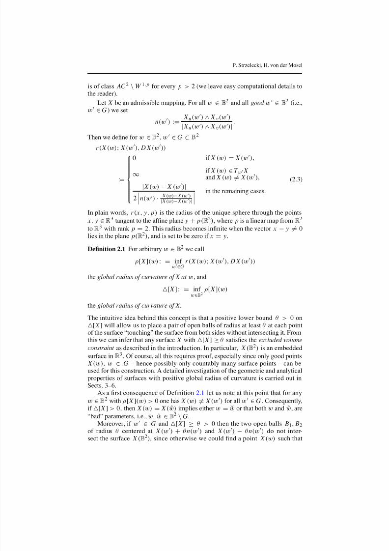
is of class AC2 \ W 1, p for every p > 2 (we leave easy computational details to

the reader).Let X be an admissible mapping. For all w ∈ B 2 and all good w ∈ B 2 (i.e.,w ∈ G ) we set

n(w ) := X u (w )

∧ X v (w )

| X u (w )∧

X v (w )|.

Then we dene for w ∈ B 2 , w ∈ G ⊂ B 2

r ( X (w) ; X (w ), D X (w ))

:=

0 if X (w) = X (w ) ,

∞ if X (w) ∈ T w X

and X (w) = X (w ) ,

| X (w)

− X (w )

|2 n(w ) · X (w) − X (w )

| X (w) − X (w )|in the remaining cases.

(2.3)

In plain words, r ( x , y, p) is the radius of the unique sphere through the points x , y ∈ R 3 tangent to the afne plane y + p(R 2) , where p is a linear map from R 2

to R 3 with rank p = 2. This radius becomes innite when the vector x − y = 0lies in the plane p(R 2) , and is set to be zero if x = y.

Denition 2.1 For arbitrary w ∈ B 2 we call

ρ [ X ](w) : = inf w∈

Gr ( X (w) ; X (w ), D X (w ))

the global radius of curvature of X at w , and

[ X ]: = inf w∈

B 2 ρ[ X ](w)

the global radius of curvature of X.

The intuitive idea behind this concept is that a positive lower bound θ > 0 on

[ X ] will allow us to place a pair of open balls of radius at least θ at each pointof the surface “touching” the surface from both sides without intersecting it. Fromthis we can infer that any surface X with [ X ] ≥ θ satises the excluded volumeconstraint as described in the introduction. In particular, X (B 2) is an embeddedsurface in R 3 . Of course, all this requires proof, especially since only good points X (w), w ∈ G – hence possibly only countably many surface points – can beused for this construction. A detailed investigation of the geometric and analyticalproperties of surfaces with positive global radius of curvature is carried out in

Sects. 3–6.As a rst consequence of Denition 2.1 let us note at this point that for any

w ∈ B 2 with ρ[ X ](w) > 0 one has X (w) = X (w ) for all w ∈ G . Consequently,if [ X ] > 0, then X (w) = X ( ˜w) implies either w = ˜w or that both w and ˜w , are“bad” parameters, i.e., w, ˜w ∈ B 2 \ G .

Moreover, if w ∈ G and [ X ] ≥ θ > 0 then the two open balls B1 , B2of radius θ centered at X (w ) + θ n(w ) and X (w ) − θ n(w ) do not inter-sect the surface X (B 2) , since otherwise we could nd a point X (w) such that




r ( X (w) ; X (w ), D X (w )) < θ contradicting our assumption on [ X ]. We shall

sometimes call B1 , B2 excluded or forbidden balls.Since G was only required to be a dense (so possibly just countable) subset of B 2 , the set B 2 \ G of bad parameters could have full measure, which necessitatesa careful investigation of the geometric and analytical properties of surfaces withpositive global curvature, see Sects. 3 – 6.

Remark. Notice that for admissible mappings X ∈ A (B 2 , R d ) , d > 3, the globalradius of curvature [ X ]can be dened analogously. The denition of r ( x , y, p)remains unchanged. There is, however, one notable difference. For every goodparameter w in the domain we have now — instead of two excluded touchingballs centered at X (w ) ±θ n(w ) — a forbidden region

U w =q∈

Sθ,w

Bθ (q ),

where the set of centers

Sθ,w := S d −1θ ( X (w )) ∩ N w X

is given by the intersection of the round (d −1)-dimensional sphere

S d −1θ ( X (w )) = {s ∈ R d : |s − X (w )| = θ }

with the afne normal space N w X = X (w ) +( D X (w )( R 2))⊥. Thus, U w looks,roughly speaking, like a thick degenerate doughnut. We have dim N w X = d −2for good w , therefore Sθ,w is in fact a (d −3)-dimensional sphere in N w X . (Notethat for d

= 3 the centers of B1 , B2 do form a zero dimensional sphere contained

in the normal line.) Analogously to the co-dimension 1 case, U w touches T w X and is excluded for X , i.e. X (B 2) ∩U w is empty.

3 Interior continuity of the normal

Let X : B 2 → R 3 be an admissible mapping, i.e., X ∈ A (B 2 , R 3), with the prop-erty that [ X ] ≥ θ , and let ∈ (0, θ) . Assume that w ∈ B 2 is a good parameter,i.e., w ∈ G . Let

(w) : = { X (w) +tn (w) : t ∈ R }be the (afne) normal line to X at w . We set

d (w) : = dist ( X (w), X (∂ B2))

C (w) : = { p ∈ R 3 |dist ( p, (w)) = },and write π w to denote the orthogonal projection onto the (afne) tangent planeT w X with center X (w) .

To show that the normal direction to X is uniformly continuous on compactsubsets of B 2 , we need the following technical denition.




Denition. We say that X has the -stretching property at w ∈ G ⊂ B 2 iff

π w C (w) ∩ X (B 2) ∩ B2 ( X (w))

is a circle of radius in the tangent plane T w X with center X (w) .

Lemma 3.1 Assume that [ X ] ≥ θ > 0. If w ∈ G and ∈ (0, 0], where0 : = min θ, d (w)/ 2 , then X has the -stretching property at w .

This Lemma means that at every good point w the image of X stretches awayfrom X (w) in all directions parallel to T w X , as long as the distance from X (w)is comparable to θ . Intuitively, a surface with [ X ] ≥ θ cannot fold abruptlyat length scales much smaller than θ : close to every straight line through X (w)in T w X intersected with Br ( X (w)) we see points of the surface, as long asr < θ

≤ [ X

]and the boundary X (∂ B 2) is far away.

Proof. Fix w ∈ G and ∈ (0, 0]. Without loss of generality we assume that X (w) = 0 ∈ R 3 and n(w) = (0, 0, 1).

Let B1 = Bθ (0, 0, θ ) and B2 = Bθ (0, 0, −θ) ; we have X (B 2) ∩( B1 ∪ B2) =∅

. Since rank D X (w) = 2, the curve X (∂ Bδ(w)) is, for some sufciently smallδ ∈ (0, ) , linked with the normal line (w) .

Now, let I ⊂ C (w) \ ( B1 ∪ B2) be a xed (but otherwise arbitrary) line seg-ment contained in B2 (0) and having its endpoints on ∂ B1 and ∂ B2 . To show that X (B 2) ∩ I is nonempty, consider a homotopy (γ s )s

∈[0,1] from γ 0 = X (∂ Bδ(w))to γ 1 = X (∂ B 2(0)) , dened as a composition of X with a homotopy from ∂ Bδ(w)to ∂B 2 in B 2 \ Bδ(w) .

Let σ be the closed curve consisting of I and two segments that join the end-

points of I to 0 = X (w) . The curves γ 0 and σ are linked, whereas γ 1 and σ are not linked, for otherwise we would have dist ( X (w), γ 1) < , contrary to thedenition of 0 , see Fig. 1.

It follows that γ s must, for some s ∈ (0, 1) , contain some point p ∈ σ . Cer-tainly p ∈ B1∪

B2 . Moreover, p = 0 = X (w) since w is a good parameter. Thus, p ∈ I . This completes the proof of the lemma.

Fig. 1 Proof of the stretching property: tangent balls B1 , B2 at X (w) , and the curves σ, γ 0 , γ 1




Remark. A version of this lemma holds also for closed compact surfaces with

global radius of curvature bounded below, see Sect. 6.3.Using the above lemma, one easily proves that the normal to X has to change

in a Lipschitz continuous way on the set of good parameters: since there are manypoints of X on little segments perpendicular to T w X , the normal at w close to wcannot rotate too much, for otherwise some points of the surface would belongto the forbidden balls associated to w . Here is a quantitative statement of thisobservation.

Lemma 3.2 Let [ X ] ≥ θ > 0. If w, w ∈ B 2 are good parameters such that

| X (w) − X (w )| < min (θ, d (w)/ 2)

and α(w,w ) ∈ [0, π2 ] is the angle between the normal directions at w and w ,

thenα(w,w ) ≤5π

θ | X (w) − X (w )|. (3.1)

Proof. As before, suppose without loss of generality that

X (w) = 0, n(w) = (0, 0, 1).

Let

q1,2 = X (w ) ±θ n(w ), p1,2 = π w (q1,2),

p0 = π w ( X (w )),

where π w is the orthogonal projection onto the tangent plane to X at X (w) . One

can assume that dist ( p1 , 0) ≤ dist ( p2 , 0) . Set r : = dist ( p0 , 0) ; obviously r ≤| X (w) − X (w )| and 0 < r ≤ θ . Pick λ ≥ 0 such that

dist ( p0 , p1) = dist ( p0 , p2 ) = λ r . (3.2)

We have sin α(w,w ) = λ r /θ . Let d =√ θ 2 −λ 2r 2 .Now, if λ ≤ 10, then

2π

α(w,w ) ≤ sin α(w,w ) ≤ 10r /θ ≤ 10| X (w) − X (w )|/θ ,

so that the desired inequality holds.We shall show that the assumption λ > 10 leads to a contradiction. Since

dist ( p1 , 0) ≤ dist ( p2 , 0) , we obtain from ( 3.2 )

dist ( p1 , 0) ≤r λ 2 +1 (3.3)

(the equality holds when dist ( p1 , 0) = dist ( p2 , 0)). Let p3 be that point of thesegment [ p1 , 0] which belongs to C r (w) . By the previous lemma, there exists apoint

q3 ∈ X (B 2) ∩Cr (w) ∩ B2r ( X (w))




such that π w (q3) = p3 . We shall show that for λ > 10 the distance t : =dist (q1 , q3) is smaller than θ , which contradicts the bound [ X ] ≥ θ .Let h = dist ( X (w ), T 0 X ) and h = dist (q3 , p3 ). Since there are no pointsof the surface X in Bθ (0, 0, θ )

∪ Bθ (0, 0, −θ) , we obtain

max (h , h ) ≤ θ − θ 2 −r 2 ≤r 2

θ .

Thus, the difference of z-components of q1 and q3 does not exceed d +h +h ≤d +2r 2 /θ . We also have

dist ( p1 , p3 ) ≤r ( λ 2 +1 −1) ≤r λ −12

(the last inequality holds for all λ

≥ 34 ). Hence,

t 2 ≤ d +2r 2

θ

2

+r 2 λ −12

2

= θ 2 +4d r 2

θ +4r 4

θ 2 −r 2λ +r 2

4

≤ θ 2 +(9 −λ) r 2 as d ≤ θ and r ≤ θ

≤ θ 2 −r 2 .

Thus, q3 is a point of X in the forbidden ball Bθ (q1) , a contradiction.

The estimate of the last lemma is uniform, and the set of good parameters isdense. Thus, we immediately obtain the following.

Corollary 3.3 The normal direction has a continuous extension to all w ∈ B 2 and the estimate (3.1 ) holds for all w, w such that | X (w) − X (w )| ≤ min θ, d (w)/ 2 .

Since now we can speak of an afne normal line (w) at every point X (w) ,w ∈ B 2 , we can associate to each point on the surface a pair of open balls of radiusθ touching the surface without intersecting it:

Corollary 3.4 Let w ∈ B 2 . Then

X (B 2) ∩ B1 = X (B 2) ∩ B2 = ∅ for the two open balls B 1 , B2 centered on the normal line (w) with radius θ , and touching each other at X (w) .

Proof. If w ∈ G this was noted already as a simple consequence of Denition 2.1in Sect. 2. If w ∈ B 2 \ G , and if we assume that there is a point X ( ˜w) containedin say B1 , then we derive a contradiction as follows: Since G is a dense subsetof B 2 we can nd a sequence of parameters w j ∈ G converging to w . By thecontinuity of X on B 2 and by Lemma 3.2 we obtain convergence of the normaldirections (w j ) to (w) with respect to the Hausdorff distance. Associated with

(w j ) we obtain a sequence of pairs of balls B j 1 , B j

2 of radius θ centered on (w j )




and touching each other in X (w j ). Consequently, we obtain (relabelling B j 2 →

B j 1 if necessary) that B

j 1 → B1 with respect to the Hausdorff distance. Hence

X ( ˜w) ∈ B j 1 for j sufciently large, contradicting the fact that B j

1 ∩ X (B 2) = ∅,since B j

1 corresponds to a good parameter w j ∈ G .

4 Continuity of the normal at the boundary

From now on we assume that X is an admissible mapping, that is, X ∈ A (B 2 , R 3) ,with the additional property that it has a rectiable boundary contour X (∂ B 2) andwith [ X ] ≥ θ > 0. Moreover we suppose that the global radius of curvature

[ X |∂ B 2] of the curve X (∂ B 2) (as dened in [ 15, p. 35]) is bounded below byθ . Note carefully that from now on

[·] is used to denote two closely related

but formally different notions. We always distinguish the argument in brackets, toavoid misunderstanding.

Theorem 4.1 Let w ∈ ∂B 2 . If (w j ) j =1, 2,... ⊂ G ⊂ B 2 is a sequence of good parameters such that w j → w as j → ∞and the normal vectors

n(w j ) : = X u ∧ X v (w j )

| X u ∧ X v (w j )| j →∞−→ ν ∈ S 2 ,

then for every good parameter w ∈ B 2 such that | X (w ) − X (w) | ≤ θ/ 100 wehave

α(w,w ) ≤100

θ | X (w) − X (w )|, (4.1)

where α(w, w ) ∈ [0, π2 ]is the angle between the afne normal line (w ) and the

line (w) := { X (w) + t ν | t ∈ R }. In particular, (w) does not depend on thechoice of the sequence (w j ) .

Let us postpone the proof of this theorem for a moment, and note the followingcorollary which follows (as before) from the density of good parameters. We stickto the notation introduced above.

Corollary 4.2 The normal direction (and therefore the afne tangent plane T w X)has a continuous extension to all w ∈ B 2 and the estimate

α(w,w ) ≤500

θ | X (w) − X (w )| (4.2)

holds for all w, w ∈ B 2 such that | X (w) − X (w )| ≤ θ / 400 . Moreover, for all w ∈ B 2 we have

X (B 2) ∩ B1 = X (B 2) ∩ B2 = ∅ (4.3)

for the two open balls B 1 , B2 centered on the normal line (w) with radius θ , and touching each other at X (w) .




Remark. B1 and B2 are referred to as the boundary touching balls in the sequel.

Proof of Corollary 4.2. If one of the points X (w), X (w ) belongs to the boundarycurve X (∂ B 2) , we can apply Theorem 4.1 directly. Assume now that w, w ∈ B 2 .If | X (w) − X (w )| < min (θ, d (w)/ 2) , then the desired estimate follows fromLemma 3.2 .

Thus, let us suppose that | X (w) − X (w )| ≥ min (θ, d (w)/ 2). Then, since

| X (w) − X (w )| ≤ θ / 400, we have

d (w) = 2min (θ, d (w)/ 2) ≤ θ / 200 .

Fix some number κ > 1 and pick a point w ∈ ∂B 2 such that d (w) = | X (w) − X (w )|. Since | X (w ) − X (w )| ≤ θ

400 + θ 200 < θ/ 100, Theorem 4.1 and triangle

inequality yield

α(w,w ) ≤ α(w,w ) +α(w , w ) ≤100

θ (d (w) + | X (w ) − X (w )|). (4.4)

Now, consider two cases.Case 1. If | X (w ) − X (w )| ≤ κ d (w) , then the right-hand side of ( 4.4 ) does notexceed

100 (κ +1)θ

d (w) ≤200 (κ +1)

θ | X (w) − X (w )|.Case 2. If | X (w ) − X (w )| > κ d (w) , then

| X (w) − X (w )| ≥ | X (w ) − X (w )| −d (w) ≥ (1 −κ−1 )| X (w ) − X (w )|,

and hence

d (w) + | X (w ) − X (w )| < ( 1 +κ−1 )| X (w ) − X (w )|≤

κ +1κ −1 | X (w ) − X (w) |.

Choosing κ = 3/ 2, in either case we estimate the right-hand side of ( 4.4 ) by500

θ | X (w ) − X (w) |, and inequality ( 4.2 ) follows.To prove the second statement (i.e. the existence of excluded touching balls

also at the boundary), one mimics the proof of Corollary 3.4 .

Proof of Theorem 4.1. Since the whole proof is rather long (yet elementary),we describe roughly the main idea. First, we prove that if the surface contains a

point X (w ) , w ∈ B 2 close to X (w) , then it contains also lots of other points X (w ) lying very close to some half-circle centered at X (w) , perpendicular to νand of radius approximately | X (w) − X (w )|. This is the boundary counterpartof the stretching property from the previous section; as before, the argument is atopological one. Next, we show that the normal direction at X (w ) must be closeto ν , for otherwise the excluded balls associated to w would contain one of thepoints X (w ) constructed in the rst step of the proof. This part of the argumentis completely geometric.




With no loss of generality we assume that X (w) = (0, 0, 0) ∈ R 3 and ν =(0, 0, 1) ∈

S 2. The pairs of forbidden ballsU j : = Bθ ( X (w j ) +θ n(w j ))∪

Bθ ( X (w j ) −θ n(w j ))

converge in the Hausdorff distance, as j → ∞, toU : = Bθ (0, 0, θ )

∪ Bθ (0, 0, −θ) .

It is clear X (B 2) ∩U = ∅, for otherwise there would be points of the surface X inU j for j sufciently large. Thus, if : [0, L] → R 3 is the arc-length parametriza-tion of X (∂ B 2) such that ( 0) = X (w) , then (0) = (a , b , 0) for some a , b ∈ R .Without loss of generality suppose that (0) = (1, 0, 0) and set

V =α∈[0,2π ]

Bθ (0, θ cos α, θ sin α) .

Since [ ] ≥ θ , by [26, Thm. 1(iv)(a) and Lemma 2] we infer that X (∂ B 2) ⊂R 3 \ V . As before, let

C (w) = { p ∈ R 3 | dist ( p, (w)) = }.

Set

h ( ) = θ − θ 2 − 2 for ∈ [0, θ ]. (4.5)

Consider two narrow, rectangular patches + and − lying on the cylinder C (w) , which are dened by

± =

( x 1 , x 2 , x 3)

∈ R 3

| x 21

+ x 22

= 2 ,

| x 3

| ≤ h( ),

± x 2

≥ 2 / 2θ . (4.6)

Elementary computations show that

+ ∪ − ⊂ (R 3 \ U ) ∩V .

(In fact, the horizontal edges of ± touch the boundary of U .) Let σ ± denote twocircular arcs along which the horizontal plane { x 3 = 0} intersects ± , respec-tively. Using ( 4.6 ) one easily checks that the length

|σ + | = |σ − | = (π −2β ) ,

where β = arctan / 4θ 2 − 2 . Instead of this formula, we just use the estimate

β ≤ tan β = 4θ 2 − 2 ≤ θ for ≤ θ .

In particular, for ≤ θ / 100 we have 2 β ≤ π / 100, and therefore

|σ ± | ≥ 0.99π for ≤ θ / 100. (4.7)

Now, ± = σ ± × I , where I denotes the interval [−h ( ), h( ) ]. We shallneed the following




Claim 1. One of the following two conditions is satised:

(i) For each p ∈ σ + there is point in X (B 2) ∩({ p}× I ) ;(ii) For each p ∈ σ − there is point in X (B 2) ∩({ p}× I ) .

In other words, if π w is the orthogonal projection onto { x 3 = 0}, thenπ w ( X (B 2) ∩ + ) = σ + or π w ( X (B 2) ∩ − ) = σ −Proof of Claim 1. Assume both (i) and (ii) are false. Then, there exist two points p1 ∈ σ + and p2 ∈ σ − such that two segments, J 1 : = { p1}× I and J 2 : = { p2}× I , contain no points of the surface X . Consider the closed curve γ which consistsof J 1 and J 2 , and two other horizontal segments J 3 , J 4 that join the endpoints of J 1 and J 2 (i.e., each of J 3 , J 4 is contained in a plane { x 3 = const}, in one of theballs Bθ (0, 0, ±θ)). We have

γ

= J 1

∪ J 2

∪ J 3

∪ J 4

⊂ V .

Moreover, the curves γ and X (∂ B 2) are linked.Now, consider a homotopy (ϕt ) t

∈[0,1] which deforms the whole boundarycurve ϕ0 = X (∂ B 2) to a small loop ϕ1 located near zero, in Bs (0) \ U , wheres = h ( )/ 4. A small arc of X (∂ B 2) that contains 0 = X (w) in its interior is keptxed, and the remaining portion of X (∂ B 2) is being deformed, using the compo-sition of X with a suitable homotopy in the domain B 2 . As h( ) ≤ for all ≤ θ ,we have dist (γ , 0) ≥ h( ) ; thus it is clear that ϕ1 and γ are not linked. Hence,one of the intermediate curves ϕt must intersect γ , and this is possible only whenthere is a point of X (B 2) in J 1 = { p1} × I or in J 2 = { p2} × I , since all theremaining points of γ belong to the forbidden balls U . This contradiction ends theproof of Claim 1.

Choose an arbitrary good parameter w with

| X (w )

− X (w)

| ≤ θ / 100. Let

q1,2 = X (w ) ±θ X u ∧ X v (w )

| X u ∧ X v (w )|denote the centers of forbidden balls corresponding to w , and let

p1,2 = π w (q1, 2), p0 = π w ( X (w )) .

From now on we x = dist ( p0 , 0) and suppose w.l.o.g. that for this particular condition (i) holds. Take λ ≥ 0 such that dist ( p0 , p1) = dist ( p0 , p2 ) = λ . Wehave

sin α(w, w ) =λθ ≤

λθ | X (w) − X (w )| .

If λ ≤ 50 there is nothing more to prove. Thus, assume that λ > 50. We shallshow that this leads to a contradiction.

Claim 2. If λ > 50 then there exists a point p 3 ∈ σ + such that

min (dist ( p1 , p3), dist ( p2 , p3)) ≤ λ −18

.




Proof of Claim 2. Let c denote the circle in { x 3 = 0}which contains the arcs σ ± .

We have p0 ∈ c . Let 0 ∈ [0, π2 ] be the angle between [ p1 , p2] and the tangentline to c at p0 . We distinguish two cases.

Case 1. 0 ≤ π / 12. Introduce complex coordinates in the { x 3 = 0}plane and let

p3 = exp (i π/ 2) p0 , p3 = exp (−i π/ 2) p0 .

Without loss of generality suppose that the angle between [ p0 , p1] and [ p0 , p3]is equal to π/ 4 ± 0 (otherwise exchange the roles of p3 and p3 ). Let d =dist ( p1 , p3) . By the law of cosines,

d 2 = λ 2 2 +2 2 −2λ 2√ 2cos π4 ± 0

≤ 2(λ 2 +2 −2λ√ 2cos π3 )

≤ 2

λ −1

4

2

for every λ > 50.Similarly,

dist ( p2 , p3 ) ≤ λ −14

.

If p3 or p3 belongs to σ + , we are done. If this is not the case, then, in view of (4.7 ), the distance of p3 to an endpoint of σ + is smaller than π / 100 (and thesame holds for p3 and the other endpoint of σ + ). Claim 2 holds then with p3

equal to any point of σ + which is sufciently close to one of its endpoints.

Case 2. 0 ≥ π/ 12. Without loss of generality assume that dist ( p1 , 0) ≤dist ( p2 , 0) . By the law of cosines,

d 2

: = dist ( p1 , 0)2

= λ 2 2

+2

−2λ 2 cos π

2 −0

= 2(λ 2 +1 −2λ sin 0)

≤ 2 λ 2 −λ2 +1 .

On the other hand, dist ( p1 , 0) ≥ (λ −1) by the triangle inequality. Thus,

(λ −1)2 ≤d 2

2 ≤ λ 2 −λ2 +1 . (4.8)

Now, let p3 and p3 be the points of c at which the tangents c passing through p1 intersect c . By (4.8 ), we have

dist 2( p1 , p3) = dist 2( p1 , p3 ) = d 2 − 2

≤ 2 λ 2 − λ2 ≤ 2 λ − 1

42 . (4.9)

Thus, if p3 or p3 belongs to σ + , then we are done. Otherwise, note that the shorter of two arcs p3 p3 has the length equal to (π − 2δ) , where sin δ = / d . Using(4.8 ), we easily estimate

|arc p3 p3 | = (π −2δ) ≥ π ( 1 −sin δ) ≥ π 1 −1

λ −1.




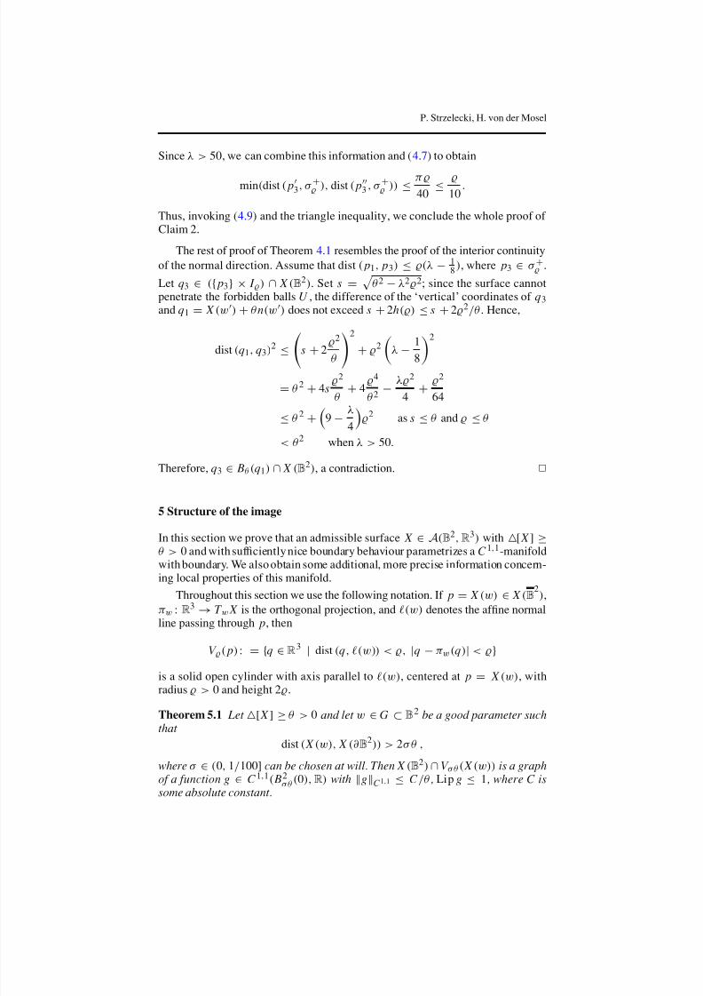
Since λ > 50, we can combine this information and ( 4.7 ) to obtain

min (dist ( p3 , σ + ), dist ( p3 , σ + )) ≤π40 ≤ 10

.

Thus, invoking ( 4.9 ) and the triangle inequality, we conclude the whole proof of Claim 2.

The rest of proof of Theorem 4.1 resembles the proof of the interior continuityof the normal direction. Assume that dist ( p1 , p3) ≤ (λ − 1

8 ) , where p3 ∈ σ + .

Let q3 ∈ ({ p3} × I ) ∩ X (B 2) . Set s = θ 2 −λ 2 2 ; since the surface cannotpenetrate the forbidden balls U , the difference of the ‘vertical’ coordinates of q3and q1 = X (w ) +θ n(w ) does not exceed s +2h ( ) ≤ s +2 2 /θ . Hence,

dist (q1 , q3)2 ≤ s +22

θ

2

+ 2 λ −18

2

= θ 2 +4s2

θ +44

θ 2 −λ 2

4 +2

64

≤ θ 2 + 9 −λ4

2 as s ≤ θ and ≤ θ

< θ 2 when λ > 50.

Therefore, q3 ∈ Bθ (q1) ∩ X (B 2), a contradiction.

5 Structure of the image

In this section we prove that an admissible surface X ∈ A (B 2 , R 3) with [ X ] ≥θ > 0 and with sufciently nice boundary behaviour parametrizes a C 1, 1-manifoldwith boundary. We also obtain some additional, more precise information concern-ing local properties of this manifold.

Throughout this section we use the following notation. If p = X (w) ∈ X (B 2) ,

π w : R 3 → T w X is the orthogonal projection, and (w) denotes the afne normalline passing through p, then

V ( p) : = {q ∈ R 3 | dist (q , (w)) < , |q −π w (q )| < }is a solid open cylinder with axis parallel to (w) , centered at p = X (w) , withradius > 0 and height 2 .

Theorem 5.1 Let [ X ] ≥ θ > 0 and let w ∈ G ⊂ B 2 be a good parameter suchthat

dist ( X (w), X (∂ B 2)) > 2σ θ ,

where σ ∈ (0, 1/ 100]can be chosen at will. Then X (B 2 ) ∩V σ θ ( X (w)) is a graphof a function g ∈ C1,1( B2

σ θ (0), R ) with g C 1,1 ≤ C /θ , Lip g ≤ 1, where C issome absolute constant.




Thus, loosely speaking, a portion of the surface contained in a cylinder of

size comparable to θ is a graph of a C1, 1

function. The norm of this function isestimated inversely proportional to θ .Before passing to the proof, we state the following.

Remark. In fact, the assumption [ X ] ≥ θ is not applied directly in the proof.What matters is the existence of excluded touching balls for every point in X (B 2) ,as given in Corollary 3.4 , and Lipschitz continuity (w.r.t. to distances measuredin the image) of the normal direction (w) . Thus, Theorem 5.1 applies to anycontinuous surface for which the excluded balls exist at every point in the image,and the line joining their centers varies in a Lipschitz continuous way. Theoriginal parametrization is not really important here.

Proof. We can assume

X (w) = 0 ∈ R 3 , n(w) = (0, 0, 1).

Since X has the -stretching property for : = σ θ , there is a point of X (B 2) ∩ B (0) on each line parallel to (w) (= the x 3-axis) such that dist ( , (w)) <σ θ . In fact, there is at most one such point (otherwise it is easy to use Lemma 3.2to obtain a contradiction).

So, if z = ( x , y) ∈ B2σ θ (0) ⊂ T w X , and p ∈ X (B 2) ∩ V σθ (0) is the unique

point such that π w ( p) = z, then we set g(z) := p3 . In other words, g = π 3 ◦(π w | X (B 2 )∩V σρ (0) )−1 , where π 3 is the projection of R 3 onto the x 3-axis.

Step 1. Since X (B 2) is contained in the complement of excluded balls at X (w) ,we have

|g(z)| ≤ |z|2 , z ∈ B2σ θ (0),

and hence g(z) = g(0) + Dg (0)z +o(|z|) as |z| → 0,

with Dg (0) = (0, 0) . At any other point z ∈ B2σ θ (0) a similar argument works:

the graph of g is trapped between two mutually tangent balls of radius θ that toucheach other at (z, g(z)) ∈ R 3 . This implies differentiability of g everywhere.Step 2. The vector ( Dg (z), 1) is parallel to the normal direction to X at w whenz = π w ( X (w )) . By Lemma 3.2 , for each w such that X (w ) ∈ V (0) we have

α(w,w ) ≤5πθ | X (w) − X (w )| ≤

5πθ ·2σ θ <

π4

.

Since tan α(w, w ) = | Dg (z)|, we have | Dg (z)| ≤ 1 everywhere in B2σ θ (0). Thus,

g is Lipschitz with Lipschitz constant 1.

Step 3. Fix two points z1 , z2 ∈ B2σ θ (0) and set a = g x (z1), b = g y(z1) ,

c = g x (z2), d = g y(z2) . The angle α between the normal directions to X (B 2)at (zi , g(zi )) , i = 1, 2, satises

sin 2 α =(a −c)2 +(b −d )2 +(ad −bc )2

(1 +a 2 +b2)( 1 +c2 +d 2)(Step 2)

≥(a −c)2 +(b −d )2

4 = | Dg (z1) − Dg(z2 )|24

. (5.1)




Suppose now that

| Dg (z1) − Dg(z2)| ≥ K |z1 −z2| (5.2)for some constant K . As g has Lipschitz constant 1, this yields

| Dg (z1) − Dg (z2)| ≥ K 2 |z1 −z2| + |g(z1) −g(z2)| . (5.3)

Combining inequalities ( 5.1 ) and (5.3 ) with the estimate of sin α resulting fromLemma 3.2, we obtain K / 4 ≤ 5π/θ . Hence Dg is Lipschitz with constant20π/θ .

There is also a boundary counterpart of the last theorem:

Theorem 5.2 Let p ∈ X (∂ B 2) , where X ∈ A (B 2 , R 3) is an admissible surfacewith [ X ] ≥ θ and [ X ∂B 2] ≥ θ for some θ > 0. Assume that X ∂B 2 : ∂B 2 → X (∂ B 2) is weakly monotone. Then, there exists a function g

∈ C1, 1( B2

θ/ 300(0))

such that g C 1, 1 ≤ C /θ , Lip g ≤ 1,

X (B2) ∩V θ/ 300 ( p) = Graph (g +bd ) ,

where B 2θ/ 300 (0) is a diskin T w X and +bd = {( x , y) ∈ B2

θ/ 300 (0) : y ≥ ψ ( x )} for some function ψ of class C 1, 1(R ) with ψ ( 0) = ψ (0) = 0 and ψ C 1,1 ≤ C /θ .

Proof. Fix p = X (w) ∈ X (∂ B 2) . Assume w.l.o.g. that p = 0 ∈ R 3 and that thelimit of normal directions to X at p coincides with the x 3 axis. Let

π w : R 3 → T w X ≡ { x 3 = 0}be the orthogonal projection onto T

w X . Set

= θ / 300.

Step 1: denition of ψ . Assume w.l.o.g. that X (∂ B 2) has an arc-lengthparametrization : [− L/ 2, L/ 2] → R 3 with ( 0) = p, (0) = (1, 0, 0) . Letγ = π w[ X (∂ B 2) ∩ V ( p)]; the curve γ ⊂ B2(0) ⊂ R 2 ≡ T w X is parametrizedby ( 1 , 2 , 0) . Since

| ( t ) − (s )| ≤1θ | ( t ) − ( s)|,

we obtain in particular 1 ≥ 1( t ) ≥ 99/ 100 and | 2(t )| ≤ 1/ 100 for all t suchthat ( t ) ∈ V ( p) . Inverting 1 , we see that γ = Graph ψ for some function ψof one variable, ψ ( 0) = ψ (0) = 0, ψ C 1,1 ≤ C /θ . (See e.g. the appendix of Norton’s paper [ 24] for a version of the Implicit and Inverse Function theorem in

Holder classes.)Step 2: we claim that π w X (B 2 )∩V ( p) is 1–1 . This follows easily from Theorem 4.1 .

Indeed, let X (w ) = ( x 1 , x 2 , x 3) ∈ V ( p) . Take the ‘vertical’ segment

I = {( x 1 , x 2 , t ) : |t | ≤ θ −(θ 2 − x 21 − x 22 )1/ 2 }which passes through X (w ) and has both endpoints on the forbidden balls as-sociated to p = X (w) . An elementary computation shows that I \ { X (w )} is




contained in (the interior of) forbidden balls associated to X (w ). Thus, X (w ) is

the only point in the image of X intersected with I ; the claim follows.Step 3. We claim that π w X (B 2) ∩V ( p) is equal either to

+ = {( x , y) ∈ B2(0) | y > ψ( x )}or to − = {( x , y) ∈ B2(0) | y < ψ( x )} (i.e. a portion of the surface near pprojects onto only one side of γ ).

Assume w.l.o.g. that + ∩ π w[ X (B 2) ∩ V ( p)] is nonempty. Then + ⊂π w[ X (B 2) ∩V ( p)], for otherwise we could nd either

(A) a piece γ 1 of X (∂ B 2) entering the cylinder V ( p) in such a waythat + ⊃ π w (γ 1) = graph ψ ,

or (B) a parameter w ∈ B 2 such that q = X (w ) belongs to

+ ∩∂(π w ( X (B 2) ∩V ( p))).

However, (A) would contradict the assumption [ X |∂ B 2] ≥ θ > 0 and thedescription of X (∂ B 2) obtained in Step 1 above. (B) implies that the normal at qmust be perpendicular to the x 3-axis, whereas | X (w) − X (w )| < 2 , which is acontradiction to ( 4.1 ).

If −∩π w[ X (B 2) ∩V ( p)] = ∅, then we are done. If this is not the case, wecan assume — repeating the reasoning above — that − ⊂ π w[ X (B 2 ) ∩V ( p)].We shall show that this assumption leads to a contradiction.

To this end, we rst note the following:

If w ∈ int B 2 , then X (w ) ∈ X (∂ B 2) ∩V ( p) . (5.4)

We prove this by contradiction. Assume that X (w ) = q ∈ X (∂ B 2) ∩V ( p) . Pickδ, r > 0 such that

Br (q ) ⊂ V ( p), (5.5)

δ < ( 1 − |w |)/ 2 and X ( Bδ (w )) ⊂ Br (q ). (5.6)

Moreover, X ( Bδ(w )) must be contained in the complement of the forbidden ‘dou-ble hose’ formed by the boundary touching balls at X (w ) and nearby points of X (∂ B 2) .

Now, two cases are possible.

(C1) X ( Bδ(w )) projects both onto + and −.

Then, ‘above’ + a portion of X ( Bδ(w )) must overlap with a portion of X ( Bδ (w )) , where w ∈ ∂B 2 and X (w ) = q = X (w ) . (We cannot have twodifferent layers of the surface in V ( p), see Step 2!). This is impossible, sincegood parameters are dense, and cannot be mapped to image points of other pa-rameters.




(C2) X ( Bδ(w )) projects only to one side of graph ψ , say to −.

Then, using the proximity of normal directions at all points of X ( Bδ (w )) to thenormal at q = X (w ) , we see (precisely as above) that the piece X ( Bδ(w )) canhave neither two different layers contained in V ( p) nor a doubly covered part,which again leads to a contradiction.

Thus, ( 5.4 ) is established.Now, take an arbitrary point q ∈ X (∂ B 2) ∩V ( p) . Since both + and − are

covered by the projection of X (B 2) ∩V ( p) , we can use ( 5.4 ) to nd two differentparameters w+, w − ∈ ∂B 2 such that X (w +) = X (w −) = q, and the imageof a small neighbourhood of w± projects onto ±, respectively. As X is weaklymonotone, a whole closed arc σ ⊂ ∂B 2 joining w + to w − satises X (σ ) = p.We use uniform continuity of X to nd an ε > 0 so small that

X ( Bε (σ )

∩B 2 )

⊂ V ( p).

Now, in the interior of Bε (σ ) ∩ B 2 we can easily nd a curve σ that joins twopoints w1 , w 2 such that

π w ( X (w 1)) ∈ +, π w ( X (w 2)) ∈ −.

By continuity, σ must contain a point w0 ∈ B 2 which is mapped by X to the boundary curve X (∂ B 2) This contradicts ( 5.4 ), and nally proves that

− ∩π w[ X (B 2 ∩V ( p)]is empty, completing Step 3 of the proof.Step 4. From now on we assume w.l.o.g. that

π w[ X (B 2) ∩V ( p)] = + ⊂ B2(0).

Then we dene g

: +

→ R , setting

g(z) = q3 when q = (q1 , q2 , q3 ) ∈ X (B 2) ∩V ( p) is such that π w (q ) = z.

Step 5. Replacing Lemma 3.2 by Theorem 4.1 in all arguments, one proves theexistence of Dg (z) for all z and the estimate | Dg (z)| ≤ 1 precisely as in theprevious Theorem. Lipschitz continuity of Dg and the estimate g C 1,1 ( +) ≤C /θ follows (one mimicks the last part of the proof of Theorem 5.1 ).Step 6. To extend g from + to the whole disk B2(0) without increasing toomuch its C 1,1-norm, we apply [ 13, Lemma 6.37].

Example. An open rotational cylinder with two hemispheres of the same radiusattached at both ends shows that C 1,1-regularity is optimal for surfaces, for whichpairs of excluded touching balls exist in the image: this particular surface fails tobe C 2 at all points where the hemispheres meet the cylinder.

Combining both theorems, we obtain the following.

Corollary 5.3 Assume that X satises the assumptions of Theorem 5.2 . Thereexist two absolute constants σ 0 > 0, K ≥ 1 such that for each σ ≤ σ 0 and p ∈ X (B 2

) we have

K −1σ 2θ 2 ≤ H 2( Bσθ ( p) ∩ X (B 2)) ≤ K σ 2θ 2 . (5.7)




In plain words, pieces of the surface in a ball of radius δ θ have their area

comparable to the area of a at disk of radius δ.Moreover, we have the following.

Lemma 5.4 Under the assumptions of Theorem 5.2 , X (B 2) is homeomorphic toa closed disk (and hence orientable).

Proof. Set A := X (B 2). It follows from the proof of Theorem 5.2 that ∂B 2 ismapped onto ∂ A ≈ S 1 in a weakly monotone (= degree one) way. Thus, thereexists a homotopy H : S 1 ×[0, 1] → ∂ A such that

H (ei θ , 0) = X (ei θ ), H (ei θ , 1) = ϕ (ei θ ) for all θ ∈ [0, 2π ],where ϕ is a xed 1–1 parametrization of ∂ A.

We argue by contradiction. Assume that A is not homeomorphic to the disk.Then, A cannot be homeomorphic to the M obius band M , as contracting ∂ B 2 toa point in B 2 and using X to transport this homotopy to the image, we wouldobtain a homotopy from a point in M to a loop that circumvents ∂ M once, whichis impossible.

Thus, A must be some other C1,1-surface (orientable or not) with boundaryhomeomorphic to S 1 . We now close the hole in A. To this end we identify R 3 witha hyperplane R 3 × {0} in R 4 , take another copy U of a closed disk and a mapY : U → R 4 , with Y ∂U identical to the boundary values of X , to attach this diskto A along ∂ A. Using H , we dene Y by the formula

Y (w) = H

w

|w |, 2 −2|w | , 1 − |w | if |w | ∈

12

, 1 ,

(2

|w

|ϕ( w

|w

|), 1

− |w

|) if

|w

| ∈0,

1

2,

(0, 0, 0, 1) if w = 0.

(5.8)

Let denote the new surface thus obtained.Glueing U and the original disk B 2 along their boundaries, we obtain a map

f : S 2 → , equal to X on one hemisphere and to Y on the other one. Since A is neither a disk nor a M¨ obius band, is different from S 2 and the projectiveplane RP 2 . Therefore, the second homotopy group π 2( ) vanishes, see e.g. [ 8,p. 198], and the map f is homotopic to the constant map. Thus, the Z 2-degree(=degree mod 2) of f , which is well dened also for non-orientable surfaces [ 8,pp. 102–106], should be zero.

However, it follows from the denition of f and Y that each point p in f (V ) ,V := B1/ 2(0), has its fourth coordinate p4 ∈ [1

2 , 1]. Since A lies in the hyperplane

{ p4 = 0} ⊂ R 3

, one easily checks that f −1

( p) is contained only in V and consistsof a single point. Thus, the Z 2-degree of f equals 1, a contradiction.

The theorems of this section show how strong in fact the assumption [ X ] ≥θ > 0 is. Even if the global curvature radius of the boundary curve γ := X (∂ B 2)is positive, γ can be badly knotted. However, if we know in addition that γ boundsa surface X ∈ A (B 2 , R 3) with [ X ] ≥ θ > 0, then it follows from Theorems 5.1and 5.2 that γ cannot be knotted! This is vaguely reminiscent of the famous F´ ary– Milnor theorem [ 22], [7, p. 402] relating curvature to topological aspects.




6 Convergence and compactness

6.1 Sets of positive reach

Following Federer [ 10, Sect. 4] we dene the reach of a set A ⊂ R d as

reach ( A) := sup{r ∈ R : ∀ x ∈ Br ( A) ∃1a ∈ A with dist ( x , A) = | x −a |}.Hence for any x ∈ Br ( A) , r < reach ( A), there is a unique next point a ≡

A( x ) ∈ A, such that dist ( x , A) = | x − A( x )|. If the set A ⊂ R d is closed, thenthe map A(.) : Breach ( A) ( A) → A is continuous, cf. [ 10, Thm. 4.8 (4)]. Given aset A ⊂ R d and a point a ∈ A one can dene the tangent cone T a A as

T a A := {v ∈ R d : v = 0

or

∀ > 0

∃b

∈ A

∩ B (a ) such that b−a

|b−a | − v

|v| <

},

which reduces to the classical (linear, not afne!) tangent plane T a , if A = ⊂R d is a C 1-submanifold in R d (cf. [ 10, Rmk. 4.6] ). Federer characterizes closedsets of positive reach by an inequality reecting a uniform second order contactbetween the set and its tangent cone:

Theorem 6.1 [10, Thm. 4.18] For a closed set A ⊂ R d and t ∈ (0, ∞) one has reach ( A) ≥ t if and only if

2 dist (b −a , T a A) ≤|b −a |2t

for all a , b ∈ A. (6.1)

Returning to our setting of admissible surfaces X ∈ A (B 2 , R 3) we can now

easily proveLemma 6.2 Let X ∈ A (B 2 , R 3) with [ X ] > 0 and [ X ∂ B 2] > 0 and θ > 0.Then the following two statements are equivalent:

(i) [ X ] ≥ θ and [ X ∂ B 2] ≥ θ ,(ii) reach ( X (B 2)) ≥ θ and reach ( X (∂ B 2)) ≥ θ .

Proof. Let A := X (B 2) and notice that A is a compact subset of R 3 since X ∈C 0(B 2 , R 3). Assume (i) and take a point x ∈ Bθ ( A). If x ∈ A simply dene

A( x ) := x , otherwise one has dist ( x , A) > 0, since A is closed. Hence thereis at least one point a ∈ A, such that | x −a | = dist ( x , A) by compactness of A.On the other hand, by Theorem 5.2 , A is a C 1,1-submanifold of R 3 . In particular,there exists a tangent plane T a A in a and a function g ∈ C1, 1(B 2

θ/ 300 (0)) with

a = g(z) for some z ∈ B 2θ/ 300 (0).Hence z furnishes a local minimum of the C 1-function h (¯z) := | x − g(¯z)|2 ,

¯z ∈ B2θ/ 300 (0). Therefore we have

0 = Dh (z) = 2( x −a ) · Dg(z),

i.e., x −a ⊥ T a A. Since dist ( x , A) < θ we conclude that x is contained in theopen segment ( y1 , y2) , where y1 and y2 are the centers of the two touching balls at




a tangent to the afne tangent plane a +T a A. If there were another point b ∈ A\{a}, such that dist ( x , A) = | x −b| < θ , then we would infer b ∈ Bθ ( y1)

∪ Bθ ( y2)contradicting Corollary 4.2 . Thus we have proved reach A ≥ θ . The second part

of the statement, i.e., reach X (∂ B 2) ≥ θ follows from [ X |∂ B 2] ≥ θ alone by [ 15,Lemma 3 (iii)].

To prove the converse notice rst that reach ( X (∂ B 2)) ≥ θ implies (again by[15, Lemma 3 (iii)] ) that [ X |∂B 2] ≥ θ . So for an indirect reasoning we canassume that [ X ] < θ, which implies that there are parameters w ∈ B 2 , w ∈ Gsuch that

0 < [ X ] ≤r :=r ( X (w) ; X (w ), D X (w )) < θ,

in particular, X (w) = X (w ) and X (w) ∈ T w X by Denition 2.1. Then d :=dist ( X (w), T w X ) satises

d

| X (w) − X (w )| = sin α,

where

α := <)( X (w) − X (w ), π w ( X (w)) − X (w )) ∈ [0, π/ 2]is the angle between the vector X (w) − X (w ) and the tangent plane T w X − X (w ) .On the other hand, by elementary geometry,

| X (w) − X (w )|2r = cos

π2 −α = sin α,

so thatd

| X (w) − X (w )| = | X (w) − X (w )|2r

,

or 2 dist ( X (w), T w X )

| X (w) − X (w )|2 =1r

contradicting ( 6.1 ) of Theorem 6.1 .

The nal result that we will need in order to investigate sequences ( X j ) j of admissible surfaces X j ∈ A (B 2 , R 3), j ∈ N , having a uniform positive lower bound on their global radius of curvature is Federer’s compactness theorem for

sets of positive reach:Theorem 6.3 [10, Thm. 4.13 & Rmk. 4.14]

Let t > 0, K ⊂ R N be compact. Then the set

{ A ⊂ K , A = ∅, reach ( A) ≥ t }is compact with respect to the Hausdorff distance.




6.2 Geometric convergence and compactness

In this section we prove two theorems on compactness and convergence of sur-faces with uniform global curvature and area/diameter bounds. We state these re-sults for disk type surfaces only. For closed compact surfaces the situation is infact simpler, see Theorem 7.2 and the remarks in the next section.

It is known in differential geometry that appropriate uniform bounds on vol-ume, injectivity radius and (some sort of) curvature lead — in much greater gener-ality than considered here — to compactness of families of Riemannian metrics,see e.g. Berger’s book [ 4, Sects. 12.4 and 11.5] and references therein, or the re-cent work of Anderson et al. [ 1, Sect. 3]. We use similar ideas in a simple context.However, since we work below the C 2-category, any direct use of (classically un-derstood) curvature is impossible. Federer’s compactness theorem and the resultsof Sect. 5 provide replacements for this gap.

Theorem 6.4 Let X j : B 2 → R 3 be a sequence of admissible surfaces with

[ X j ] ≥ θ > 0. Assume moreover that:

(i) sup j H2( X j (B 2 )) ≤ M < +∞;

(ii) X j ∂B 2 are weakly monotone and parametrize rectiable Jordancurves with global radius of curvature uniformly bounded belowby θ , and there exists some R > 0 such that each of the curves X j (∂ B 2) contains a point p j ∈ B R(0) .

Then one can select a subsequence j such that A j : = X j (B 2) converge in Hausdorff distance to A, A is a C 1, 1-manifold with boundary, and the nearest point projection π A : Bθ ( A) → A is well dened.

Corollary 6.5 Under the assumptions of Theorem 6.4, one can choose a subse-quence which satises also

H 2( X j (B 2)) → H 2( A).

Theorem 6.6 Let a sequence ( X j ) j ⊂ A (B 2 , R 3) satisfy [ X j ] ≥ θ > 0 and

[ X j ∂ B 2] ≥ θ , and let X j ∂B 2 be weakly monotone parametrizations of theboundary curves X j (∂ B 2) . Assume also that X ∈ C0(B 2 , R 3) and that X j (∂ B 2)converges to X (∂ B 2) in Hausdorff distance.

If X j (w) → X (w) as j → ∞ for all w belonging to some dense subset of B 2 ,then

(i) the X j are uniformly bounded;

(ii) the sets A j : = X j (B2) converge in Hausdorff distance to a C

1, 1-

manifold A with reach A ≥ θ , and we have A = X (B 2) .

Remarks. 1. It follows from our proofs that in both theorems above the limit man-ifold A is also equipped with local graph representations whose norms and sizesare uniformly controlled by θ , as described in Sect. 5. Moreover, Corollary 3.4holds for A, that is, we have two touching balls B1 and B2 at every point of A, and A ⊂ R 3 \ ( B1 ∪ B2).




2. The uniform area bound in the assumptions of Theorem 6.4 is satised e.g.

when sup j X j W 1,2 ≤ M < +∞. The second part of assumption (ii), i.e. the ex-istence of a point p j ∈ X j (∂ B 2)∩ B R(0) , is obviously satised when the boundarycontours converge to a xed curve or are themselves xed (as often encounteredin the calculus of variations).3. In fact, it follows from the initial steps of our proof that for any family of admissible surfaces G such that all X ∈ G are weakly monotone on ∂B 2 andsatisfy min ( [ X ], [ X ∂ B 2]) ≥ θ > 0, we have

sup X ∈

Gdiam X (B 2) < +∞ ⇔ sup

X ∈

GH 2( X (B 2)) < +∞. (6.2)

Similarly, for any family C of Jordan curves such that [γ ] ≥ θ > 0 for all γ ∈ C we have

supγ ∈

C diam γ < +∞ ⇔ supγ ∈

C H1(γ) < +∞. (6.3)

Proof of Theorem 6.4 . The overall strategy is as follows. We rst show that all A j := X j (B 2) are uniformly bounded, and all boundary curves γ j := X j (∂ B 2)have uniformly bounded length. Then, applying Federer’s compactness theorem,we select subsequences of A j , γ j that converge in Hausdorff distance to A and γ .Finally, we cover A and γ by two nite families F A and F γ of open balls, andexploit Theorems 5.1 and 5.2 to see that in each of these balls A j coincides with agraph (or a piece of graph) of a C 1, 1-function. Hausdorff convergence combinedwith norm estimates for these functions allows to apply the Arzela–Ascoli com-pactness theorem and to conclude nally that A is a C 1,1-manifold with boundary.

We now present the details.

Step 1: all A j := X j (B 2) are contained in a xed ball B ˜ R(0) ⊂ R 3 . To seethis, x j and consider the covering { Bσ 0 θ ( p) | p ∈ A j } of A j , where σ 0 isgiven by Corollary 5.3. Apply Vitali’s lemma to this covering to obtain a (possiblynite) sequence of pairwise disjoint balls Bσ 0 θ ( pk ), where pk ∈ A j , such that

{ B5σ 0 θ ( pk ) | k = 1, 2, . . . } is a covering of A j . Take N of these balls. Invoking(5.7 ) for each of them, and summing w.r.t. k , we obtain

N K −1σ 20 θ 2 ≤ N

k =1

H 2( Bσ 0 θ ( pk ) ∩ A j ) ≤ H 2( X j (B 2)) ≤ M .

This yields N ≤ K M σ −20 θ −2 , and next diam ( X j (B 2

)) ≤ 10 K M σ −10 θ −1 . By (ii),

there is some

˜ R > 0 such that

j X j (B 2

)

⊂ B

˜ R(0) .

Step 2: length bounds for γ j . To show that all γ j = X (∂ B 2) have uniformlybounded length, notice rst that

H 1(γ ∩ Bθ/ 8( p)) ≤ θ (6.4)

whenever p ∈ γ and γ is a Jordan curve in R 3 with [γ ] ≥ θ > 0. Indeed, let be the arc length parametrization of γ . Suppose w.l.o.g. that ( 0) = 0 = p,




(0) = (1, 0, 0) . We have the uniform estimate | ( t ) − (s )| ≤ θ −1|t −s|, and

this implies for the rst coordinate 1 of :

1(s ) >12

for all s ∈ (−θ/ 2, θ / 2) .

Thus, estimating the rst coordinate of , we obtain

( ±θ/ 2) ∈ Bθ/ 4( p) (6.5)

and thereforeγ ∩ Bθ/ 4( p) ⊂ ([−θ/ 2, θ/ 2]),

which leads to ( 6.4 ), since (τ) ∈ Bθ/ 8( p) for all τ ∈ [−θ/ 2, θ / 2]. To see thelatter suppose there existed another curve point q := (τ) ∈ Bθ / 8( p) with τ ∈[−θ/ 2, θ/ 2]. Then (since is injective due to [γ ] ≥ θ > 0 and [15, Lemma 1])

0 < dist (q , (

[−θ/ 2, θ / 2

])) < θ/ 8,

but |q − ( ±θ/ 2)| ≥ θ / 8 by (6.5 ). This implies that there is a next point (τ ∗)with τ ∗ ∈ (−θ/ 2, θ / 2) such that

dist (q , ( [−θ/ 2, θ/ 2])) = |q − (τ ∗)|,from which we infer that q − (τ ∗) ⊥ (τ ∗) . (Note that is of class C 1,1 by[26, Thm. 1(iii)]. ) But this means that q = (τ) is contained in the union of ballsof radius θ touching γ in (τ ∗) contradicting [ 26, Thm. 1(iv)(a)].

A uniform length bound is now obtained by an application of Vitali’s lemmato the covering of γ j by balls Bθ/ 40 ( p) , p ∈ γ j : we select an at most countablesubfamily of pairwise disjoint balls Bθ/ 40 ( pk ) , pk ∈ γ j , such that larger balls Bθ/ 8( p) , pk ∈ γ j , cover γ j . Now, the sum of volumes of Bθ/ 40 ( pk ) does notexceed the volume of B R

+θ (0) , since each γ j

⊂ B R(0) by Step 1. This yields the

uniform bound 1 ≤ k ≤ K , where K ≤ const ( R+θ)3θ −3 . Next, (6.4 ) for γ := γ j implies that

H 1(γ j ) ≤k

H 1(γ j ∩ Bθ/ 8( pk )) ≤ K θ for all j .

Step 3: Hausdorff convergence of γ j and A j . Applying Federer’s compactnesstheorem (Theorem 6.3) twice, which is possible due to Lemma 6.2 , we select asubsequence (still labeled by the index j ) such that

γ j → γ , A j → A in Hausdorff distance , (6.6)

and the reaches of γ and A are ≥ θ . Moreover, the uniform length bound for γ j

allows us to use the results of [ 26, Sect. 4] to conclude that γ is a Jordan curvewith [γ ] ≥ θ and C 1,1 arc length parametrization .Step 4: covering γ and A by good patches. We x an ε > 0 small, to be speciedlater on. From now on we assume that

dist H (γ j , γ ) +dist H ( A j , A) ≤12

εθ for all j , (6.7)

passing to a subsequence if necessary.




We also suppose w.l.o.g. that R ≥ θ , where A j ⊂ B R(0) for all j . To exploit

the results of Sect. 5, we construct two nite families of disjoint balls,F

γ andF

A,with the following properties:

(i) F γ = { B100 εθ ( pk ) | pk ∈ γ for k = 1, . . . , K }(ii) card F γ = K R3(εθ) −3

(iii) The union K

k =1

B500 εθ ( pk ) contains the set

B100 εθ (γ )∪

∞

j =1

B99εθ (γ j ), (6.8)

i.e., enlarging the balls from F γ we obtain a covering of tubular neighbour-

hoods of γ and all γ j .(iv) F A = { B4εθ (qm ) | qm ∈ A\ B90εθ (γ ) for m = 1, . . . , N }(v) card F A = N R3(εθ) −3

(vi) The union M

m=1

B20εθ (qm ) contains the set

B4εθ ( A \ B100εθ (γ )). (6.9)

and each of the sets

Bεθ ( A j \ B99εθ (γ j )) j = 1, 2, . . . (6.10)

To obtain these families, we apply the Vitali lemma twice, rst to the covering

{ B100 εθ ( p) | p ∈ γ } of a tubular neighbourhood of γ , and then to the coveringof a tubular neighbourhood of A \ B100 εθ (γ ) . Conditions (i)–(iii) are immediate;the cardinality bound (ii) is obtained precisely as in Steps 1 and 2 of the proof.

To justify (v), we argue as follows: each qm is a limit of q jm ∈ A j , and by(6.7 ) we can assume that |q jm −qm | < εθ/ 2 for each m ; thus, for each xed j the balls B3εθ (q jm) are pairwise disjoint. Now, an argument analogous to the onecarried out in Step 1 above shows that for a xed small ε the index m can takeonly nitely many values.

Finally, condition (vi) follows from Vitali’s lemma and the inclusions

Bεθ ( A j \ B99εθ (γ j )) ⊂ B2εθ ( A \ B98εθ (γ)) ⊂ B4εθ ( A \ B100 εθ (γ )),

which can be obtained from ( 6.7 ) and the triangle inequality. Note that the unionof all the balls B500 εθ ( pk ) and B20εθ (qm ) covers the whole of A.

Step 5: convergence of normals at the centers of small patches. We next select for each j points p jk ∈ γ j and q jm ∈ A j \ B99εθ (γ j ) so that

p jk → pk , q jm → qm for all k , m; (6.11)

| p jk − pk | + |q jm −qm| < εθ/ 2 for all j , k , m. (6.12)

Moreover, for each xed j the union of the balls B501 εθ ( p jk ), 1 ≤ k ≤ K , coversthe tubular neighbourhoods ( 6.8 ). Similarly, the union of the balls B21εθ (q jm)




covers A j \ B99εθ (γ j ). This follows from (iii) and (vi) in Step 4, and from ( 6.12 ).

We also have B501 εθ ( p jk ) ⊂ B502 εθ ( pk ), B21εθ (q jk ) ⊂ B22εθ (qm ),

since the centers p jk and q jm are close to pk and qm , respectively.Let n jm ∈ S 2 be normal to A j = X j (B 2) at q jm =: X j (w jm), and let n jk ∈

S 2 be normal to A j at p jk =: X j (w jk ) , w jk ∈ ∂B 2 . Selecting nitely manysubsequences, we may assume that for all k , m

n jm → νm ∈ S 2 and n jk → νk ∈ S 2 as j → ∞, (6.13)

|n jm −νm| + |n jk −νk | < δ for all j = 1, 2 . . . and all k , m. (6.14)

Now, select ε = 10−6 ; Theorems 5.1 and 5.2 can then be applied in balls of

radius smaller than 1000 εθ . Last step: the structure of A. Fixing δ > 0 sufciently small in ( 6.14 ), and denot-ing by V m the cylinder with center qm , axis parallel to νm , diameter r := 21εθ andheight 2 r , we invoke Theorem 5.1 to conclude that for each j and m

A j ∩V m

is a nice open patch of the graph of

g jm : B221εθ (qm ) → R

where B221εθ (qm ) denotes a xed 2-dimensional disk, centered at qm and con-

tained in the plane passing through qm and perpendicular to νm (i.e. in the planewhich is the limit of T w jm X j as j

→ ∞). By Theorem 5.1, we have g jm

∈ C 1,1 ,

g jm C 1,1 ≤ const /θ and Lip (g jm) ≤ 2. (Notice that for each xed m we slightlytilt these graphs, to x their common planar domain.)

Since the Lipschitz norms of all Dg jm are uniformly bounded, by the Arzela– Ascoli theorem we may assume, selecting nitely many subsequences if neces-sary, that g jm → gm as j → ∞ in the C 1-topology, for each xed m. Moreover,each gm is of class C 1, 1 since the Lipschitz condition for Dg jm is preserved in thelimit j → ∞.Thus, A\ B100 εθ (γ ) is covered by nitely many graphs of C 1,1-functions gm .Moreover, it follows form Hausdorff convergence of A j → A and γ j → γ ,and from the C 1-convergence g jm → gm that each point in this part of A has aneighbourhood U (whose size scales like θ ) such that A∩U is in fact a graph of a C 1,1-function from a disk to R .

We repeat a similar argument at the boundary, applying Theorem 5.2 insteadof Theorem 5.1. As a result, we obtain C 1,1-functions

f jk : B2501 εθ ( pk ) → R ,

dened on disks in the planes that pass through pk and are perpendicular to νk ,such that pieces of A j in small neighbourhoods of pk are equal to graphs of f jk re-stricted to + jk given by Theorem 5.2. Passing to subsequences as before, we con-clude that for each k the set A∩ B501 εθ ( pk ) is C 1,1-diffeomorphic to a semidisk.




Hence c lies on the segment of H j parallel to ν j , which implies

π j (c) = H j ∩(q j +T q j A j ),

where π j denotes the orthogonal projection onto the afne tangent plane q j +T q j A j . Now ( 6.21 ) leads to

dist (π j (c), B2θ/ 300 \ − j ) ≥ 2r ,

but (6.22 ) on the other hand would give |π j (c) − π j (a )| < 2r , a contradiction,since π j (a ) ∈ B2

θ/ 300 \ − j . Hence ( 6.21 ) holds true.

Now connect c1 j (1) and c2

j (1) with the endpoints q j ± 4r ν j (q j ) of H j bystraight segments of length θ −4r to obtain τ j . By (4.3 ) of Corollary 4.2 appliedto X j and by ( 6.21 ) we nd

dist (τ j , A j ) ≥ 2r for all j ∈ N , (6.23)

which, together with ( 6.16 ) and (6.19 ) implies ( 6.17 ). Relation ( 6.18 ) follows from(6.15 ), (6.23 ), (6.16 ) and (6.19 ) as well by virtue of the Hausdorff convergence X j (∂ B 2) → X (∂ B 2) as j → ∞, since 8 r < θ/ 300 < R/ 600 .

This convergence and ( 6.21 ) imply also that the curves c j are non-triviallylinked with X (∂ B 2) for j sufciently large, because c j is linked with X j (∂ B 2)for each j ∈ N by construction. Therefore c j ∩ X (B 2) = ∅ for all j 1 as X ∈ C 0(B 2 , R 3) is of disk-type.

Let X (w j ) ∈ c j ∩ X (B 2) . We may take a subsequence to obtain w j → w ∈ B 2 .If w ∈ ∂B 2 , then X (w) ∈ X (∂ B 2) , and by continuity

dist ( X (w j ), X (∂ B2)) < r for all j 1,

contradicting ( 6.18 ). Hence w ∈ B 2 . Then Br / 4( X (w)) ⊂ Br / 2(c j ) for all j 1.By continuity of X we nd δ > 0 such that X ( Bδ(w)) ⊂ Br / 2(c j ) for all j 1.Since we have assumed pointwise convergence X j → X on a dense subset of B 2

we nd w ∈ Bδ(w) such that X j (w ) → X (w ) as j → ∞, in particular

X j (w ) ∈ Br (c j ) for all j 1. (6.24)

On the other hand by ( 6.15 )

X j (w ) ∈ B R+r (0) for all j 1. (6.25)

But ( 6.24 ) together with ( 6.25 ) contradict ( 6.17 ) as r < R/ 4800, which concludes

the proof of (i).(ii) Since the X j are uniformly bounded by (i) we may apply Federer’s com-

pactness theorem, Theorem 6.3 , to get a subsequence A j := X j (B 2) convergingin Hausdorff distance to a set A ⊂ R 3 with reach A ≥ θ, which implies that A isclosed (cf. [ 10, Rmk. 4.2] ). Since X j → X on a dense subset of B 2 as j → ∞we obtain X (w) ∈ A for all w contained in that dense subset of B 2 . By continuitywe nd X (B 2 ) ⊂ A, since A is closed.




Now take j even larger if necessary to have

| X j (w ) − X (w )| < r / 4, | p j − p| < r / 4

to obtain X (w ) ∈ B5r / 8( p) which contradicts ( 6.26 ). Thus we have shown that X (B 2) = A.

We are now in the situation of Theorem 6.4 , where assumption (i) was appliedonly to derive a uniform diameter bound for the X j (B 2) , which we have shown inPart (i) of the present theorem. Hence A = X (B 2) is a C 1,1 -manifold with bound-ary. Since X was xed from the beginning we may conclude from the subsequenceprinciple that the whole sequence A j converges to A in Hausdorff distance.

7 Ideal surfaces

In this section we apply the previously obtained regularity and compactness resultsto prove the existence of the so-called ideal surfaces.

Fix θ > 0, g ≥ 1 and a closed, compact reference surface M g of genus gthat is smoothly embedded in R 3 in such a way that its tubular neighbourhoodhas width ≥ θ (i.e. the nearest point projection M : p

∈ M Bθ ( p) → M is well

dened). We consider the class

S θ ( M g ) = { X ∈ A ( M g , R 3) : [ X ] ≥ θ , X ( M g )iso

M g} (7.1)

of thick admissible surfaces that are (ambiently) isotopic to M g . (See e.g. [16,Vol. 5, p. 209] for the denition of isotopy.) Clearly, S θ ( M g ) is nonempty as theidentity mapping belongs to it.

Theorem 7.1 For each g = 1, 2, . . . , each θ > 0 and each xed reference surface M g satisfying the above assumptions, the class S θ ( M g ) contains a surface of minimal area.

Basically, this result follows from the geometric compactness, Theorem 6.4 inthe previous section and its Corollary 6.5 . However, these two results have beenstated only for disk type surfaces, therefore we indicate briey the changes thatneed to be introduced in various regularity results in Sects. 3–5, to adapt them tocompact closed surfaces of genus g ≥ 1.

Remark 1. The stretching property, Lemma 3.1. The claim of this lemma stillholds at every good parameter w ∈ M g ; we can take 0 := θ as there is no

boundary. Indeed, R3

\ X ( M g ) has two connected components U 1 and U 2 ; see e.g.Lima’s paper [ 20] for a clever proof for general compact closed hypersurfaces inR d +1 . We have ∂U 1 = ∂U 2 = X ( M g ) . One of the excluded balls B1 , B2 at X (w)is contained in U 1 , and the other one in U 2 . Thus, any segment I ⊂ R 3 \ ( B1∪

B2)with one endpoint on ∂ B1 and the other endpoint on ∂ B2 must contain atleast one point of the common boundary of U 1 and U 2 , i.e., a point of thesurface.




Remark 2. The proofs of interior continuity of the normal (cf. Sect. 3) and the

description of the local graph structure (cf. Sect. 5) of X ( M g ) remain unchanged.All the arguments there rely only on the stretching property, on the existence of excluded touching balls, and on elementary geometry. In fact, everything simpli-es a bit, as there is no boundary. In particular, for each point p ∈ X ( M g ) theintersection of V θ/ 100 ( p) and X ( M g ) is isometric to the graph of a C 1,1-function f with Lip f ≤ 1, f C 1,1 ≤ C /θ . The area estimates of Corollary 5.3 also holdtrue.

After these preparations, we are ready to state and prove the following.

Theorem 7.2 Each sequence of surfaces X j ∈ S θ ( M g ) , j = 1, 2, . . . , such that

sup j ∈

N

H 2( X j ( M g )) < +∞contains a subsequence X j such that

(i) X j ( M g ) converge (in Hausdorff distance and in C 1-topology) to aclosed compact C 1, 1-surface A ⊂ R 3 that satises

reach A ≥ θ ;(ii) H 2 ( X j ( M g )) → H 2( A) as j → ∞;

(iii) A has genus g and moreover Aiso

X j ( M g ) for all j sufcientlylarge.

Proof. Conditions (i) and (ii) are obtained precisely in the same way as

Theorem 6.4 and Corollary 5.3 . In fact, the proof of compactness shortens a bit,as we do not have to care about the boundaries of surfaces. (One just needs Step 1,i.e., a uniform diameter bound for all A j := X j ( M g ) , then an application of Federer’s compactness theorem yields convergence of some subsequence of A j in the Hausdorff distance, next a good nite covering is constructed by a simpli-ed version of Step 3, and nally, passing to convergent subsequences of normalsand applying Arzela–Ascoli’s theorem, we obtain local C 1-convergence of graphpatches that cover A j to graph patches that cover A.)

Thus, we only have to prove (iii). This is done in two steps. For sake of sim-plicity we denote the selected subsequence again by X j .Step 1. The genus of A is equal to g , as A is homotopically equivalent to X j ( M g )for all j sufciently large (see Dubrovin, Novikov and Fomenko, [ 8, Ch. 17], for the denition and its consequences). To check the equivalence, we x j so large

thatdist H ( A j , A) <

θ 2

. (7.2)

Let f := A A j

, g := A j A. (7.3)

We shall show that f ◦g id A and g ◦ f id A j , where denotes the homotopyof maps.




For every x ∈ A we have

| x −g( x )| < θ/ 2, |g( x ) −g( f ( x )) | < θ/ 2

by ( 7.2 ). Hence, | x − f (g( x )) | < θ and the whole closed segment with endpoints x , f (g( x )) is contained in Bθ ( A) , i.e. in the domain of A. The homotopy f ◦g id A is given by

H t ( x ) = A tx +(1 −t ) f (g( x )) for x ∈ A and t ∈ [0, 1].The homotopy g ◦ f id A j is constructed in a similar way.Step 2. There exists an isotopy that carries a neighbourhood of A to a neighbour-hood of A j (and A to A j ) for j 1.

Set, for p ∈ R 3 and ν ∈ S 2 , I r ( p, ν) := { p +t ν : |t | < r / 2}. Let

N j := Bθ/ 2( A j ) = p∈

A j I θ ( p, ν j ( p)), (7.4)

where ν j is a xed vector eld normal to A j = X j ( M g ), and

N j := p∈

A j

I θ A j A−1( p), ν j ( p) . (7.5)

To prove that N j is an open neighbourhood of A and to dene the desired isotopy,we check rst that

A j A: A → A j

is bijective for all j 1.To check injectivity, assume the contrary: for innitely many j there exist

points p j 1 = p j 2 ∈ A with A j ( p j 1 ) = A j ( p j 2 ) = q j ∈ A j . Thus, by the triangleinequality,

| p j 1 − p j

2 | ≤ 2 dist H ( A j , A) → 0 as j → ∞.Passing to a subsequence if necessary, we can assume that p j

1 , p j 2 → p ∈ A as

j → ∞. Now, p j 1 , p j

2 belong to the line j (q j ) normal to A j at q j . It follows fromthe C 1 -convergence of local graph patches of A j to graph patches of A that the

j (q j ) is close to ( p j 1 ) , the normal to A at p j

1 . In particular, if δ > 0 is xed, then

the excluded balls associated to A at p j 1 contain two segments of j (q j ) having

common length at least 4 θ −δ for j 1. Therefore, p j 2 belongs to one of these

balls and is different from p j 1 , a contradiction.To check surjectivity, consider

J j = { x ∈ A j | ∃ p( x ) ∈ A : A j ( p( x )) = x }.

This set is nonempty as A ⊂ Bθ ( A j ) for all j large. Closedness of J j followsimmediately from closedness of A j and A and continuity of the projection.Finally,

J j = { x ∈ A j | x = A j ( A ∩ I 2θ ( x , ν j ( x ))}




and A intersects, for j 1, all ‘needles’ I θ ( x , ν j ( x )) transversally because of the

C1-convergence proven in (i), so if it intersects one of them, it must intersect allnearby ones. Thus, J j is open in A j . As A j is connected, we have J j = A j , i.e.,

A j A is surjective onto A j .This implies that N j is an open neighbourhood of A for j 1.

We can now nally dene : N j × [0, 1] → R 3 by

( x , τ ) = x +τ A j ( x ) − A j A−1( A j ( x )) . (7.6)

Thus, the map ( ·, τ ) restricted to an arbitrary line orthogonal to A j agrees witha translation. It is a straightforward exercise to check that

(a) ( N j , 1) = N j ,

(b) ( ·, 0) = id N j ,(c) ( ·, τ ) is, for each τ ∈ [0, 1], a homeomorphism whose inverse is given by

ξ → ξ −τ A j (ξ ) − A j A−1( A j (ξ)) ,

(d) ( A, 1) = A j .

Hence, is the desired isotopy.

Proof of Theorem 7.1. We pick a minimizing sequence and apply Theo-rem 7.2. (One can parametrize the limiting surface by a composition of X j and

( ·, 1)−1 .)

Acknowledgements This work has been started while the rst author was enjoying the freedomof being a Humboldt Fellow in Bonn; he gratefully acknowledges the generosity of the Alexan-der von Humboldt Foundation. The rst author was also partially supported by KBN grant no.2 PO 3A 028 22. The second author enjoyed the hospitality of Professor John Maddocks andof the Centre Bernoulli at the EPFL Lausanne during Spring 2003 and Spring 2004. We wouldalso like to thank the Sonderforschungsbereich 611 at the University of Bonn for supporting our research.

References

1. Anderson, M., Katsuda, A., Kurylev, Y., Lassas, M., Taylor, M.: Boundary regularity for the Ricci equation, geometric convergence, and Gelfand’s inverse boundary problem. Inv.Math. 58, 261–321 (2004)

2. Banavar, J.R., Gonzalez, O., Maddocks, J.H., Maritan, A.: Self-interactions of strands and

sheets. J. Statist. Phys. 110 , 35–50 (2003)3. Banavar, J.R., Maritan, A., Micheletti, C., Trovato, A.: Geometry and physics of proteins.Proteins 47, 315–322 (2002)

4. Berger, M.: A panoramic view of Riemannian geometry. Springer-Verlag, Berlin (2003)5. Bonk, M., Lang, U.: Bi-Lipschitz parameterization of surfaces. Math. Annalen 327 , 135–

169 (2003)6. Dierkes, U., Hildebrandt, S., K uster, A., Wohlrab, O.: Minimal Surfaces I, II. Grundlehren

math. Wiss. 295 & 296 , Springer Berlin (1992)7. do Carmo, M.P.: Differential geometry of curves and surfaces. Prentice-Hall, Inc., Engle-

wood Cliffs, N.J. (1976)




8. Dubrovin, B.A., Fomenko, A.T., Novikov, S.P.: Modern geometry—methods and applica-tions. Part II. The geometry and topology of manifolds. Graduate Texts in Mathematics,104. Springer-Verlag, New York (1985)

9. Durumeric, O.C.: Thickness formula and C 1 compactness for C 1,1 Riemannian submani-folds. ArXiv: math.DG/0204050 (2002)

10. Federer, H.: Curvature measures. Trans. Amer. Math. Soc. 93, 418–491 (1959)11. Freedman, M.H., Zheng-Xu, He., Zhenghan, W.: M obius energy of knots and unknots. Ann.

of Math. (2) 139 , 1–50 (1994)12. Fu, J.H.G.: Bi-Lipschitz rough normal coordinates for surfaces with an L1 curvature bound.

Indiana Univ. Math. J. 47, 439–453 (1998)13. Gilbarg, D., Trudinger, N.: Elliptic partial differential equations of second order. Second

edition. Grundlehren der math. Wiss. 224 , Springer Berlin (1983)14. Gonzalez, O., Maddocks, J.H.: Global Curvature, Thickness, and the Ideal Shape of Knots.

The Proceedings of the National Academy of Sciences, USA 96(9), 4769–4773 (1999)15. Gonzalez, O., Maddocks, J.H., Schuricht, F., von der Mosel, H.: Global curvature and self-

contact of nonlinearly elastic curves and rods. Calc. Var. Partial Differential Equations 14,29–68 (2002)

16. Hazewinkel, M.: (ed.) Encyclopaedia of mathematics. Kluwer, Dodrecht (1990)17. He, Zheng-Xu.: The Euler-Lagrange equation and heat ow for the M obius energy. Comm.

Pure Appl. Math. 53, 399–431 (2000)18. Kusner, R.B., Sullivan, J.M.: M obius-invariant knot energies. Ideal knots , 315–352, Ser.

Knots Everything, 19, World Sci. Publishing, River Edge, NJ (1998)19. L eger, J.C.: Menger curvature and rectiability. Ann. of Math. (2) 149 , 831–869 (1999)20. Lima, Elon L.: Orientability of smooth hypersurfaces and the Jordan–Brouwer separation

theorem. Expo. Math. 5, 283–286 (1987)21. Mal y, J.: Absolutely continuous functions of several variables. J. Math. Anal. Appl. 231(2),

492–508 (1999)22. Milnor, J.W.: On the total curvature of knots. Ann. of Math. 52, 248–257 (1950)23. M uller, S., Sver ak, V.: On surfaces of nite total curvature. J. Differential Geom. 42, 229–

258 (1995)24. Norton, A.: A critical set with nonnull image has large Hausdorff dimension. Trans. Amer.

Math. Soc. 296 , 367–376 (1986)25. O’Hara, J.: Energy of a knot. Topology 30, 241–247 (1991)26. Schuricht, F., von der Mosel, H.: Global curvature for rectiable loops. Math. Z. 243 , 37–77

(2003)27. Schuricht, F., von der Mosel, H.: Euler-Lagrange equations for nonlinearly elastic rods with

self-contact. Arch. Rat. Mech. Anal. 168 , 35–82 (2003)28. Schuricht, F., von der Mosel, H.: Characterization of ideal knots. Calc. Var. Partial Differ-

ential Equations 19, 281–305 (2004)29. Seifert, U.: Fluid membranes — theory of vesicle conformations. Ber. Forschungszentrum

Julich 2997 (1994)30. Semmes, S.: Hypersurfaces in Rn whose normal has small BMO norm. Proc. Amer. Math.

Soc. 112 , 403–412 (1991)31. Strzelecki, P., von der Mosel, H.: On a Mathematical Model for Thick Surfaces. Phys-

ical and Numerical Models in Knot Theory , 547–564, Ser. Knot Everything, 36, WorldScientic, Singapore 2005

32. Toro, T.: Surfaces with generalized second fundamental form in L2 are Lipschitz manifolds.J. Differential Geom. 39, 65–101 (1994)

global curvature for surfaces and area minimization under a thickness constraint

Documents