GLMM tutoR

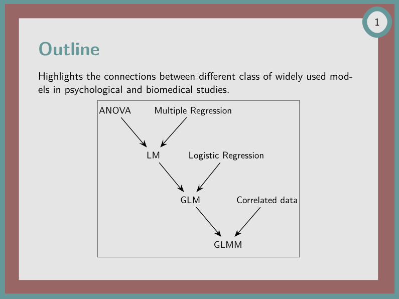
OutlineHighlights the connections between different class of widely used mod-els in psychological and biomedical studies.

ANOVA Multiple Regression

LM Logistic Regression

GLM Correlated data

GLMM

1

Overview of GLMMCompared to standard (generalized) linear models, mixed-effect modelsfurther include random-effect terms that allow to reflect correlationbetween statistical units. Such clustered data may arise as the resultof grouping of individuals (e.g., students nested in schools), within-unitcorrelation (e.g., longitudinal data), or a mix thereof (e.g., performanceover time for different groups of subjects) [1, 2, 3, 4, 5].Typically, this approach fall under the category of conditional models,as opposed to marginal models, like GLS or GEE, where we are inter-ested in modeling population-averaged effects by assuming a working(within-unit) correlation matrix.Mixed-effect models are not restricted to a single level of clustering,and they give predicted values for each cluster or level in the hierarchy.

2

Available tools in R

In preparation: Bates and coll., lme4: Mixed-effects Modeling with R,http://lme4.r-forge.r-project.org/book/

3

Fixed vs. random effectsThere seems to be little agree-ment about what fixed andrandom effects really means:http://bit.ly/Jd0EiZ, butsee also [6].As a general decision work-flow, we can ask whether weare interested in just estimat-ing parameters for the random-effect terms, or get predic-tions at the individual level [7,p. 277].

Is it reasonable to assume levels of the factor come froma probability distribution?

No Yes

Treat factor as fixed Treat factor as random

Where does interest lie?

Only in the distribution ofthe random effects

In both the distribution andthe realized values of the

random effects

Estimate parameters of the distribution of the random effects

Estimate parameters of the distribution of the random effects and calculate predictors of realized values of the

random effects

4

Analysis of paired dataThe famous “sleep” study [8] is a good illustration of the importance ofusing pairing information when available.

Test assuming independent subjectsTest acknowledging pairing

t.test(extra ~ group, data=sleep)t.test(extra ~ group, data=sleep, paired=TRUE)

Generally, ignoring within-unit correlation results in a less powerful test.Why? We know that

Var(X1 −X2) = Var(X1) + Var(X2)− 2Cov(X1, X2)

(Cov(X1, X2) = ρ√

Var(X1)√

Var(X2)).Considering that Cov(X1, X2) = 0 amounts to over-estimate varianceof the differences, since Cov(X1, X2) will generally be positive.

5

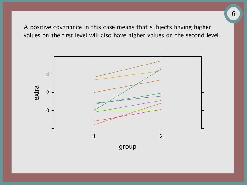
A positive covariance in this case means that subjects having highervalues on the first level will also have higher values on the second level.

group

extra

0

2

4

1 2

6

Analysis of repeated-measuresPill type

SubjectID None Tablet Capsule Coated average

1 44.5 7.3 3.4 12.4 16.92 33.0 21.0 23.1 25.4 25.63 19.1 5.0 11.8 22.0 14.54 9.4 4.6 4.6 5.8 6.15 71.3 23.3 25.6 68.2 47.16 51.2 38.0 36.0 52.6 44.5

Pill typeaverage 38.1 16.5 17.4 31.1 25.8

Lack of digestive enzymes in the intes-tine can cause bowel absorption prob-lems, as indicated by excess fat inthe feces. Pancreatic enzyme supple-ments can be given to ameliorate theproblem [7, p. 254].

There is only one predictor, Pill type, which is attached to subject andperiod of time (subsumed under the repeated administration of the dif-ferent treatment).

7

Variance componentsTwo different ways of decomposing the total variance:

One-way ANOVATwo-way ANOVA

RM ANOVA

aov(fecfat ~ pilltype, data=fat)aov(fecfat ~ pilltype + subject, data=fat)aov(fecfat ~ pilltype + Error(subject),

data=fat)

Source DF SS MS M1 M2*/M3

pilltype 3 2009 669.5 669.5/359.7 669.5/107.0p=0.169 p=0.006

subject 5 5588 1117.7 — 1117.7/107.0p=0.000*

Residuals 15 1605 107.0 — —

The first model, which assumesindependent observations, doesnot remove variability betweensubjects (about 77.8% of resid-ual variance).

The last two models incorporate subject-specific effects:yij = µ+ subjecti + pilltypej + εij, εij ∼ N (0, σ2

ε)

In the third model, we further assume subjecti ∼ N (0, σ2s), indepen-

dent of εij.

8

Variance components (Con’t)The inclusion of a random effect specific to subjects allows to modelseveral types of within-unit correlation at the level of the outcome.What is the correlation between measurements taken from the sameindividual? We know that

Cor(yij, yik) = Cov(yij, yik)√Var(yij)

√Var(yik)

.

Because µ and pilltype are fixed, and εij ⊥ subjecti, we have

Cov(yij, yik) = Cov(subjecti, subjecti)

= Var(subjecti)

= σ2s ,

and variance components follow from Var(yij) = Var(subjecti) +Var(εij) = σ2

s + σ2ε , which is assumed to hold for all observations.

9

So that, we have

Cor(yij, yik) = σ2s

σ2s + σ2

ε

which is the proportion of the total variance that is due to subjects. Itis also known as the intraclass correlation, ρ, and it measures the close-ness of observations on different subjects (or within-cluster similarity).

• Subject-to-subject variability simultaneously raises or lowers all theobservations on a subject.

• The variance-covariance structure in the above model is called com-pound symmetry:

σ2s + σ2

ε σ2s σ2

s σ2s

σ2s σ2

s + σ2ε σ2

s σ2s

σ2s σ2

s σ2s + σ2

ε σ2s

σ2s σ2

s σ2s σ2

s + σ2ε

= σ2

1 ρ . . . ρρ 1 ρ...

. . ....

ρ ρ . . . 1

.(σ2 = σ2

s + σ2ε)

10

Estimating ρObservations on the same subject are modeled as correlated throughtheir shared random subject effect. Using the random intercept modeldefined above, we can estimate ρ as follows:

Load required packageFit a random intercept model

ANOVA tableGet approximate 95% CIs

σs

σε

ρ=0.7025066

library(nlme)lme.fit <- lme(fecfat ~ pilltype, data=fat,

random= ~ 1 | subject)anova(lme.fit)intervals(lme.fit)sigma.s <- as.numeric(VarCorr(lme.fit)[1,2])sigma.eps <- as.numeric(VarCorr(lme.fit)[2,2])sigma.s^2/(sigma.s^2+sigma.eps^2)

It should be noted that REML method is used by default: random effects are estimatedafter having removed fixed effects. Tests for random effects (H0 : σ2 = 0) with LRTare conservative.

11

Estimating ρ (Con’t)From the ANOVA table, we can also extract the relevant variance com-ponents to get the desired ρ:

Extract variance components

Subjects varianceResidual variance

ρ=0.7025066

ms <- anova(lm(fecfat ~ pilltype + subject,data=fat))[[3]]

vs <- (ms[2] - ms[3])/nlevels(fat$pilltype)vr <- ms[3]vs / (vs+vr)

Notice that we could also use Generalized Least Squares, imposingcompound symmetry for errors correlation:

Fit GLS model

ANOVA tableρ=0.7025074

gls.fit <- gls(fecfat ~ pilltype, data=fat,corr=corCompSymm(form= ~ 1 | subject))

anova(gls.fit)intervals(gls.fit)

12

The imposed variance-covariance structure is clearly reflected in thepredicted values.

Pill type

Feca

l fat

(g/d

ay)

0

20

40

60

Tablet Capsule Coated None

Pill type

Pre

dict

ed fe

cal f

at (g

/day

)0

20

40

60

Tablet Capsule Coated None

13

Model diagnosticInspection of the distribution of the residuals and residuals vs. fittedvalues plots are useful diagnostic tools. It is also interesting to examinethe distribution of random effects (intercepts and/or slopes).

Standard normal quantiles

Residuals

-10

-5

0

5

10

15

-2 -1 0 1 2

Fitted values

Residuals

-10

-5

0

5

10

15

0 10 20 30 40 50 60

14

Some remarks• For a balanced design, the residual variance for the within-subject

ANOVA and random-intercept model will be identical (the REMLestimator is equivalent to ANOVA MSs). Likewise, Pill type effectsand overall mean are identical.

• Testing the significance of fixed effects can be done using ANOVA(F-value) or by model comparison. In the latter case, we need to fitmodel by ML method (and not REML) because models will includedifferents fixed effects.

ANOVA tableRefit base model by ML

Intercept-only model

LRT=14.6 (p=.0022)

anova(lme.fit)lme.fit <- update(lme.fit, method="ML")lme.fit0 <- update(lme.fit,

fixed= . ~ - pilltype)anova(lme.fit, lme.fit0)

• Parametric bootstrap may be used to compute a more accurate p-value for the LRT (here a χ2(3)), see [9, pp. 158–161].

15

Variance-covariance structureOther VC matrices can be choosen, depending on study design [10,pp. 232–237], e.g. Unstructured, First-order auto-regressive, Band-diagonal, AR(1) with heterogeneous variance.The random-intercept model ensures that the VC structure will be con-strained as desired. With repeated measures ANOVA, a common strat-egy is to use Greenhouse-Geisser or Huynh-Feldt correction to correctfor sphericity violations, or to rely on MANOVA which is less power-ful, e.g. [11, 12] (see also http://homepages.gold.ac.uk/aphome/spheric.html).Mixed-effect models are more flexible as they allow to make inferenceon the correlation structure, and to perform model comparisons.

16

Longitudinal dataAverage reaction time per day for subjects in a sleep deprivation study. On day 0 the subjects had their normal amountof sleep. Starting that night they were restricted to 3 hours of sleep per night. The observations represent the averagereaction time on a series of tests given each day to each subject. D. Bates, Lausanne 2009, http://bit.ly/Kj8VVj

Days of sleep deprivation

Ave

rage

reac

tion

time

(ms)

200250300350400450

02468

310 309

02468

370 349

02468

350 334

02468

308 371

02468

369

351

02468

335 332

02468

372 333

02468

352 331

02468

330

200250300350400450

337

17

Results from simple linear regressionIndividual regression lines (N = 18):

(Intercept) Days25% 229.4167 6.19454875% 273.0255 13.548395

Subjects exhibit different response pro-files, and overall regression line is:

y = 251.4 + 10.5x.How well does this equation captureobserved trend (across subjects)?

Days

Fitte

d re

actio

n tim

e

200

250

300

350

400

450

0 1 2 3 4 5 6 7 8

• OLS estimates are correct, but their standard errors aren’t (becauseindependence is assumed).

• Individual predictions will be incorrect as well.

18

Some plausible models• Random-intercept model

Reaction ~ Days + (1 | Subject)

• Random-intercept and slope modelReaction ~ Days + (Days | Subject)

• Uncorrelated random effects (intercept and slope)Reaction ~ Days + (1 | Subject) + (0 + Days | Subject)

Models:lme.mod1: Reaction ~ Days + (1 | Subject)lme.mod3: Reaction ~ Days + (1 | Subject) + (0 + Days | Subject)lme.mod2: Reaction ~ Days + (Days | Subject)

Df AIC BIC logLik Chisq Chi Df Pr(>Chisq)lme.mod1 4 1802.1 1814.9 -897.05lme.mod3 5 1762.0 1778.0 -876.02 42.0525 1 8.885e-11 ***lme.mod2 6 1764.0 1783.1 -875.99 0.0609 1 0.8051

19

Predicting random effectsIn a model with random effects, the corresponding regression coeffi-cients are no longer parameters and cannot be estimated as is done inusual linear models. Moreover, their expectation is zero. However, itis possible to rely on their posterior distribution (Bayesian approach).Combining conditional modes of the random effects and estimates ofthe fixed effects yields conditional modes of the within-subject coeffi-cients. See also lme4::mcmcsamp.It is easy to check that predicted random effects are related to fixedeffects.

Two-way ANOVA

Extract fixed-effects

Constant ratio (0.9349347)

lm.mod1 <- aov(Reaction ~ Days + Subject,data=sleepstudy)

subj.fixef <- model.tables(lm.mod1,cterms="Subject")[[1]]$Subject

ranef(lme.mod1)$Subject/subj.fixef

20

Predicted valuesyi = ( β0︸︷︷︸

Fixed

+ u0i︸︷︷︸Random

) + (β1 + u1i)x

Days of sleep deprivation

Ave

rage

reac

tion

time

(ms)

200250300350400450

02468

310 309

02468

370 349

02468

350 334

02468

308 371

02468

369

351

02468

335 332

02468

372 333

02468

352 331

02468

330

200250300350400450

337

Mixed model Within-group

21

Shrinkage of within-unit coefficientsPredicted values from random-effect modelsare shrinkage estimators. For simple cases, itamounts to

τ = σ2u

σ2u + σ2

ε/ni,

where ni is the sample size for the ith cluster.Here, τ = 37.12/(37.12 + 31.02/10) = 0.935.There will be little skrinkage when statisticalunits are different, or when measurements areaccurate, or with large sample.

Days

Fitte

d re

actio

n tim

e

200

250

300

350

400

450

0 1 2 3 4 5 6 7 8

Random effects: Reaction Days Subject predGroups Name Variance Std.Dev. 1 249.5600 0 308 292.1888Subject (Intercept) 1378.18 37.124 2 258.7047 1 308 302.6561Residual 960.46 30.991 3 250.8006 2 308 313.1234

Number of obs: 180, groups: Subject, 18 4 321.4398 3 308 323.5907...

Fixed effects: 177 334.4818 6 372 332.3246Estimate Std. Error t value 178 343.2199 7 372 342.7919

(Intercept) 251.4051 9.7459 25.80 179 369.1417 8 372 353.2591Days 10.4673 0.8042 13.02 180 364.1236 9 372 363.7264

22

Categorical and continuous predictors

Age (years)

Exe

rcis

e (h

ours

per

wee

k)

0

5

10

15

20

25

30

8 10 12 14 16 18

control

8 10 12 14 16 18

patient

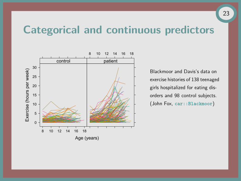
Blackmoor and Davis’s data onexercise histories of 138 teenagedgirls hospitalized for eating dis-orders and 98 control subjects.(John Fox, car::Blackmoor)

23

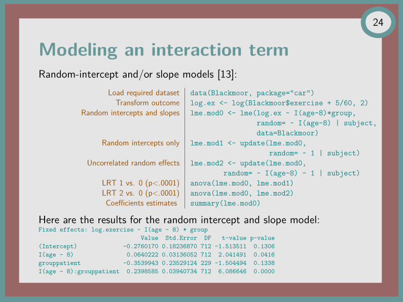
Modeling an interaction termRandom-intercept and/or slope models [13]:

Load required datasetTransform outcome

Random intercepts and slopes

Random intercepts only

Uncorrelated random effects

LRT 1 vs. 0 (p<.0001)LRT 2 vs. 0 (p<.0001)Coefficients estimates

data(Blackmoor, package="car")log.ex <- log(Blackmoor$exercise + 5/60, 2)lme.mod0 <- lme(log.ex ~ I(age-8)*group,

random= ~ I(age-8) | subject,data=Blackmoor)

lme.mod1 <- update(lme.mod0,random= ~ 1 | subject)

lme.mod2 <- update(lme.mod0,random= ~ I(age-8) - 1 | subject)

anova(lme.mod0, lme.mod1)anova(lme.mod0, lme.mod2)summary(lme.mod0)

Here are the results for the random intercept and slope model:Fixed effects: log.exercise ~ I(age - 8) * group

Value Std.Error DF t-value p-value(Intercept) -0.2760170 0.18236870 712 -1.513511 0.1306I(age - 8) 0.0640222 0.03136052 712 2.041491 0.0416grouppatient -0.3539943 0.23529124 229 -1.504494 0.1338I(age - 8):grouppatient 0.2398585 0.03940734 712 6.086646 0.0000

24

Predicted valuesThe interaction between the grouping factor and continuous predictorappears clearly when predicting outcomes from the random interceptand slope model. Fox [13] also demonstrates that adding serial correla-tion for the errors will improve goodness of fit.

Age (years)

Exe

rcis

e (h

ours

per

wee

k)

1

2

3

4

5

8 10 12 14 16 18

patient control

25

Take-away message• Conditional and marginal models extend classical generalized lin-

ear models by modeling within-unit correlation, and possibly errorsstructure.

• Mixed-effect models are flexible tools that allow to draw inferenceon such correlation structures, and also compute predicted valuesat different levels of clustering. Inference on random effects requiresophisticated computational methods, though.

• Incorporating random effects and testing working hypothesis onwithin-unit correlation overcome the classical paradigm of repeatedmeasures ANOVA.

26

References[1] CE McCulloch and SR Searle. Generalized, Linear, and Mixed Models. Wiley, 2001.

[2] JK Lindsey. Models for Repeated Measurements. Oxford University Press, 2nd edition, 1999.

[3] SW Raudenbush and AS Bryk. Hierarchical Linear Models: Applications and Data Analysis Methods.Thousand Oaks CA: Sage, 2nd edition, 2002.

[4] A Gelman and J Hill. Data Analysis Using Regression and Multilevel/Hierarchical Models. CambridgeUniversity Press, 2007.

[5] GM Fitzmaurice. Longitudinal Data Analysis. CRC Press, 2009.

[6] A Gelman. Analysis of variance–why it is more important than ever. Annals of Statistics, 33(1):1–53,2005.

[7] E Vittinghoff, DV Glidden, SC Shiboski and McCulloch. Regression Methods in Biostatistics. Linear,Logistic, Survival, and Repeated Measures Models. Springer, 2005.

[8] Student. The probable error of a mean. Biometrika, 6(1):1-25, 1908.

[9] JJ Faraway. Extending the linear model with R. Chapman & Hall/CRC, 2006.

[10] JC Pinheiro and DM Bates. Mixed-Effects Models in S and S-PLUS. Springer, 2000.

[11] H Abdi. The greenhouse-geisser correction. In N Salkind, editor, Encyclopedia of Research Design.Thousand Oaks, CA: Sage, 2010.

[12] JH Zar. Biostatistical Analysis. Pearson, Prentice Hall, 4th edition, 1998.

[13] J Fox. Linear mixed models. App. to An R and S-PLUS Companion to Applied Regression. 2002

27