package ‘glmm’ - r · package ‘glmm ’ february 22, 2018 ... format a data frame with the...

Package ‘glmm’February 22, 2018

Type Package

Title Generalized Linear Mixed Models via Monte Carlo LikelihoodApproximation

Version 1.2.3

Date 2018-02-19

Maintainer Christina Knudson <[email protected]>

Description Approximates the likelihood of a generalized linear mixed model using Monte Carlo like-lihood approximation. Then maximizes the likelihood approximation to return maximum likeli-hood estimates, observed Fisher information, and other model information.

License GPL-2

Depends R (>= 3.1.1), trust, mvtnorm, Matrix, digest

Imports stats

ByteCompile TRUE

NeedsCompilation yes

VignetteBuilder knitr

Suggests knitr

Repository CRAN

Author Christina Knudson [aut, cre],Charles J. Geyer [ctb]

Date/Publication 2018-02-22 17:32:16 UTC

R topics documented:bacteria . . . . . . . . . . . . . . . . . . . . . . . . . . . . . . . . . . . . . . . . . . . 2bernoulli.glmm . . . . . . . . . . . . . . . . . . . . . . . . . . . . . . . . . . . . . . . 3binomial.glmm . . . . . . . . . . . . . . . . . . . . . . . . . . . . . . . . . . . . . . . 4Booth2 . . . . . . . . . . . . . . . . . . . . . . . . . . . . . . . . . . . . . . . . . . . . 5BoothHobert . . . . . . . . . . . . . . . . . . . . . . . . . . . . . . . . . . . . . . . . 6cbpp2 . . . . . . . . . . . . . . . . . . . . . . . . . . . . . . . . . . . . . . . . . . . . 6coef.glmm . . . . . . . . . . . . . . . . . . . . . . . . . . . . . . . . . . . . . . . . . . 7confint.glmm . . . . . . . . . . . . . . . . . . . . . . . . . . . . . . . . . . . . . . . . 8

1

2 bacteria

glmm . . . . . . . . . . . . . . . . . . . . . . . . . . . . . . . . . . . . . . . . . . . . 9logLik.glmm . . . . . . . . . . . . . . . . . . . . . . . . . . . . . . . . . . . . . . . . 14mcse . . . . . . . . . . . . . . . . . . . . . . . . . . . . . . . . . . . . . . . . . . . . . 15mcvcov . . . . . . . . . . . . . . . . . . . . . . . . . . . . . . . . . . . . . . . . . . . 16murder . . . . . . . . . . . . . . . . . . . . . . . . . . . . . . . . . . . . . . . . . . . . 17poisson.glmm . . . . . . . . . . . . . . . . . . . . . . . . . . . . . . . . . . . . . . . . 18radish2 . . . . . . . . . . . . . . . . . . . . . . . . . . . . . . . . . . . . . . . . . . . . 19salamander . . . . . . . . . . . . . . . . . . . . . . . . . . . . . . . . . . . . . . . . . 20se . . . . . . . . . . . . . . . . . . . . . . . . . . . . . . . . . . . . . . . . . . . . . . 20summary.glmm . . . . . . . . . . . . . . . . . . . . . . . . . . . . . . . . . . . . . . . 21varcomps . . . . . . . . . . . . . . . . . . . . . . . . . . . . . . . . . . . . . . . . . . 23vcov.glmm . . . . . . . . . . . . . . . . . . . . . . . . . . . . . . . . . . . . . . . . . . 24

Index 25

bacteria Presence of Bacteria after Drug Treatments

Description

Tests of the presence of the bacteria H. influenzae in children with otitis media in the NorthernTerritory of Australia.

Usage

data(bacteria)

Format

A data frame with the following columns:

y Presence or absence: a factor with levels n and y.

ap active/placebo: a factor with levels a and p.

hilo hi/low compliance: a factor with levels hi and lo.

week Numeric: week of test.

ID Subject ID: a factor.

trt A factor with levels placebo, drug, drug+, a re-coding of ap and hilo.

y2 y reformatted as 0/1 rather than n/y.

Details

Dr. A. Leach tested the effects of a drug on 50 children with a history of otitis media in the NorthernTerritory of Australia. The children were randomized to the drug or the a placebo, and also to receiveactive encouragement to comply with taking the drug.

The presence of H. influenzae was checked at weeks 0, 2, 4, 6 and 11: 30 of the checks were missingand are not included in this data frame.

bernoulli.glmm 3

References

Venables, W. N. and Ripley, B. D. (2002) Modern Applied Statistics with S, Fourth edition. Springer.

Examples

data(bacteria)

bernoulli.glmm Functions for the Bernoulli family.

Description

Given a scalar eta, this calculates the cumulant and two derivatives for the Bernoulli family. Alsochecks that the data are entered correctly.

Usage

bernoulli.glmm()

Value

family.glmm The family name, as a string.link The link function (canonical link is required), as a string.cum The cumulant function.cp The first derivative of the cumulant function.cpp The second derivative of the cumulant function.checkData A function to check that all data are either 0 or 1.

Note

This function is to be used by the glmm command.

Author(s)

Christina Knudson

See Also

glmm

Examples

eta<--3:3bernoulli.glmm()$family.glmmbernoulli.glmm()$cum(eta)bernoulli.glmm()$cp(1)bernoulli.glmm()$cpp(2)

4 binomial.glmm

binomial.glmm Functions for the Binomial family.

Description

Given a scalar eta and the number of trials, this calculates the cumulant and two derivatives for theBernoulli family. Also checks that the data are entered correctly.

Usage

binomial.glmm()

Value

family.glmm The family name, as a string.

link The link function (canonical link is required), as a string.

cum The cumulant function.

cp The first derivative of the cumulant function.

cpp The second derivative of the cumulant function.

checkData A function to check that all data are nonnegative.

Note


Author(s)

Christina Knudson

See Also

glmm

Examples

eta<--3:3ntrials <- 1binomial.glmm()$family.glmmbinomial.glmm()$cum(eta, ntrials)binomial.glmm()$cp(1, ntrials)binomial.glmm()$cpp(2, ntrials)

Booth2 5

Booth2 A Logit-Normal GLMM Dataset

Description

This data set contains simulated data from the paper of Booth and Hobert (referenced below) aswell as another vector.

Usage

data(Booth2)

Format

A data frame with 3 columns:

y Response vector.

x1 Fixed effect model matrix. The matrix has just one column vector.

z1 A categorical vector to be used for part of the random effect model matrix.

z2 A categorical vector to be used for part of the random effect model matrix.

Details

The original data set was generated by Booth and Hobert using a single variance component, asingle fixed effect, no intercept, and a logit link. This data set has the z2 vector added purely toillustrate an example with multiple variance components.

References

Booth, J. G. and Hobert, J. P. (1999) Maximizing generalized linear mixed model likelihoods withan automated Monte Carlo EM algorithm. Journal of the Royal Statistical Society, Series B, 61,265–285.

Examples

data(Booth2)

6 cbpp2

BoothHobert A Logit-Normal GLMM Dataset from Booth and Hobert

Description

This data set contains simulated data from the paper of Booth and Hobert referenced below.

Usage

data(BoothHobert)

Format


y Response vector.x1 Fixed effect model matrix. The matrix has just one column vector.z1 Random effect model matrix. The matrix has just one column vector.

Details

This data set was generated by Booth and Hobert using a single variance component, a single fixedeffect, no intercept, and a logit link.

References

Booth, J. G. and Hobert, J. P. (1999) Maximizing generalized linear mixed model likelihoods withan automated Monte Carlo EM algorithm. Journal of the Royal Statistical Society, Series B, 61,265–285.

Examples

data(BoothHobert)

cbpp2 Contagious bovine pleuropneumonia

Description

This data set is a reformatted version of cbpp from the lme4 package. Contagious bovine pleu-ropneumonia (CBPP) is a major disease of cattle in Africa, caused by a mycoplasma. This datasetdescribes the serological incidence of CBPP in zebu cattle during a follow-up survey implementedin 15 commercial herds located in the Boji district of Ethiopia. The goal of the survey was to studythe within-herd spread of CBPP in newly infected herds. Blood samples were quarterly collectedfrom all animals of these herds to determine their CBPP status. These data were used to computethe serological incidence of CBPP (new cases occurring during a given time period). Some data aremissing (lost to follow-up).

coef.glmm 7

Usage

data(cbpp2)

Format


Y Response vector. 1 if CBPP is observed, 0 otherwise.

period A factor with levels 1 to 4.

herd A factor identifying the herd (1 through 15).

Details

Serological status was determined using a competitive enzyme-linked immuno-sorbent assay (cELISA).

References

Lesnoff, M., Laval, G., Bonnet, P., Abdicho, S., Workalemahu, A., Kifle, D., Peyraud, A., Lancelot,R., Thiaucourt, F. (2004) Within-herd spread of contagious bovine pleuropneumonia in Ethiopianhighlands. Preventive Veterinary Medicine, 64, 27–40.

Examples

data(cbpp2)

coef.glmm Extract Model Coefficients

Description

A function that extracts the fixed effect coefficients returned from glmm.

Usage

## S3 method for class 'glmm'coef(object,...)

Arguments

object An object of class glmm usually created using glmm.

... further arguments passed to or from other methods.

Value

coefficients A vector of coefficients (fixed effects only)

8 confint.glmm

Author(s)

Christina Knudson

See Also

glmm for model fitting.

Examples

library(glmm)set.seed(1234)data(salamander)#To get more accurate answers for this model, use m=10^4 or 10^5# and doPQL=TRUE.m<-10sal<-glmm(Mate~0+Cross,random=list(~0+Female,~0+Male),varcomps.names=c("F","M"),data=salamander,family.glmm=bernoulli.glmm,m=m,debug=TRUE,doPQL=FALSE)

coef(sal)

confint.glmm Calculates Asymptotic Confidence Intervals

Description

A function that calculates asymptotic confidence intervals for one or more parameters in a modelfitted by by glmm. Confidence intervals can be calculated for fixed effect parameters and variancecomponents using models.

Usage

## S3 method for class 'glmm'confint(object, parm, level, ...)

Arguments


parm A specification of which parameters are to be given confidence intervals, eithera vector of numbers or a vector of names. If missing, all parameters are consid-ered.

level The confidence level required.

... Additional arguments passed to or from other methods.

Value

A matrix (or vector) with columns giving lower and upper confidence limits for each parameter.These will be labeled as (1-level)/2 and 1-(1-level)/2 in percent. By default, 2.5

glmm 9

Author(s)

Christina Knudson

See Also


Examples

library(glmm)data(BoothHobert)set.seed(123)mod.mcml1<-glmm(y~0+x1,list(y~0+z1),varcomps.names=c("z1"),data=BoothHobert,family.glmm=bernoulli.glmm,m=10,doPQL=TRUE)confint(mod.mcml1)

glmm Fitting Generalized Linear Mixed Models using MCML

Description

This function fits generalized linear mixed models (GLMMs) by approximating the likelihood withordinary Monte Carlo, then maximizing the approximated likelihood.

Usage

glmm(fixed, random, varcomps.names, data, family.glmm, m,varcomps.equal, doPQL = TRUE,debug=FALSE, p1=1/3,p2=1/3, p3=1/3,rmax=1000,iterlim=1000, par.init, zeta=5)

Arguments

fixed an object of class "formula" (or one that can be coerced to that class): a sym-bolic description of the model to be fitted. The details of model specification aregiven under "Details."

random an object of class "formula" (or one that can be coerced to that class): a sym-bolic description of the model to be fitted. The details of model specification aregiven under "Details."

varcomps.names The names of the distinct variance components in order of varcomps.equal.

data an optional data frame, list or environment (or object coercible by as.data.frameto a data frame) containing the variables in the model. If not found in data, thevariables are taken from environment(formula), typically the environment fromwhich glmm is called.

family.glmm The name of the family. Must be class glmm.family. Current options arebernoulli.glmm, poisson.glmm, and binomial.glmm.

10 glmm

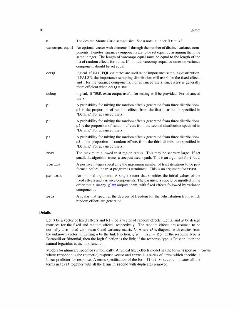
m The desired Monte Carlo sample size. See a note in under "Details."

varcomps.equal An optional vector with elements 1 through the number of distinct variance com-ponents. Denotes variance components are to be set equal by assigning them thesame integer. The length of varcomps.equal must be equal to the length of thelist of random effects formulas. If omitted, varcomps.equal assumes no variancecomponent should be set equal.

doPQL logical. If TRUE, PQL estimates are used in the importance sampling distribution.If FALSE, the importance sampling distribution will use 0 for the fixed effectsand 1 for the variance components. For advanced users, since glmm is generallymore efficient when doPQL=TRUE.

debug logical. If TRUE, extra output useful for testing will be provided. For advancedusers.

p1 A probability for mixing the random effects generated from three distributions.p1 is the proportion of random effects from the first distribution specified in"Details." For advanced users.

p2 A probability for mixing the random effects generated from three distributions.p2 is the proportion of random effects from the second distribution specified in"Details." For advanced users.

p3 A probability for mixing the random effects generated from three distributions.p3 is the proportion of random effects from the third distribution specified in"Details." For advanced users.

rmax The maximum allowed trust region radius. This may be set very large. If setsmall, the algorithm traces a steepest ascent path. This is an argument for trust.

iterlim A positive integer specifying the maximum number of trust iterations to be per-formed before the trust program is terminated. This is an argument for trust.

par.init An optional argument. A single vector that specifies the initial values of thefixed effects and variance components. The parameters should be inputted in theorder that summary.glmm outputs them, with fixed effects followed by variancecomponents.

zeta A scalar that specifies the degrees of freedom for the t-distribution from whichrandom effects are generated.

Details

Let β be a vector of fixed effects and let u be a vector of random effects. Let X and Z be designmatrices for the fixed and random effects, respectively. The random effects are assumed to benormally distributed with mean 0 and variance matrix D, where D is diagonal with entries fromthe unknown vector ν. Letting g be the link function, g(µ) = Xβ + ZU . If the response type isBernoulli or Binomial, then the logit function is the link; if the response type is Poisson, then thenatural logarithm is the link function.

Models for glmm are specified symbolically. A typical fixed effects model has the form response ~ termswhere response is the (numeric) response vector and terms is a series of terms which specifies alinear predictor for response. A terms specification of the form first + second indicates all theterms in first together with all the terms in second with duplicates removed.

glmm 11

A specification of the form first:second indicates the set of terms obtained by taking the interac-tions of all terms in first with all terms in second. The specification first*second indicates thecross of first and second. This is the same as first + second + first:second.

The terms in the formula will be re-ordered so that main effects come first, followed by the interac-tions, all second-order, all third-order and so on: to avoid this, pass a terms object as the formula.

If you choose binomial.glmm as the family.glmm, then your response should be a two-columnmatrix: the first column reports the number of successes and the second reports the number offailures.

The random effects for glmm are also specified symbolically. The random effects model specifica-tion is typically a list. Each element of the random list has the form response ~ 0 + term. The0 centers the random effects at 0. If you want your random effects to have a nonzero mean, theninclude that term in the fixed effects. Each variance component must have its own formula in thelist.

To set some variance components equal to one another, use the varcomps.equal argument. Theargument varcomps.equal should be a vector whose length is equal to the length of the random ef-fects list. The vector should contain positive integers, and the first element of the varcomps.equalshould be 1. To set variance components equal to one another, assign the same integer to the corre-sponding elements of varcomps.equal. For example, to set the first and second variance compo-nents equal to each other, the first two elements of varcomps.equal should be 1. If varcomps.equalis omitted, then the variance components are assumed to be distinct.

Each distinct variance component should have a name. The length of varcomps.names should beequal to the number of distinct variance components. If varcomps.equal is omitted, then the lengthof varcomps.names should be equal to the length of random.

Monte Carlo likelihood approximation relies on an importance sampling distribution. Though in-finitely many importance sampling distributions should yield the correct MCMLEs eventually, theimportance sampling distribution used in this package was chosen to reduce the computation cost.When doPQL is TRUE, the importance sampling distribution relies on PQL estimates (as calculatedin this package). When doPQL is FALSE, the random effect estimates in the distribution are taken tobe 0, the fixed effect estimates are taken to be 0, and the variance component estimates are taken tobe 1.

This package’s importance sampling distribution is a mixture of three distributions: a t centered at0 with scale matrix determined by the PQL estimates of the variance components and with zetadegrees of freedom, a normal distribution centered at the PQL estimates of the random effects andwith a variance matrix containing the PQL estimates of the variance components, and a normaldistribution centered at the PQL estimates of the random effects and with a variance matrix basedon the Hessian of the penalized log likelihood. The first component is included to guarantee thegradient of the MCLA has a central limit theorem. The second component is included to mirror ourbest guess of the distribution of the random effects. The third component is included so that thenumerator and the denominator are similar when calculating the MCLA value.

The Monte Carlo sample size m should be chosen as large as possible. You may want to run themodel a couple times to begin to understand the variability inherent to Monte Carlo. There are nohard and fast rules for choosing m, and more research is needed on this area. For a general idea, Ibelieve the BoothHobert model produces stable enough estimates at m = 103 and the salamandermodel produces stable enough estimates at m = 105, as long as doPQL is TRUE.

To see the summary of the model, use summary().

12 glmm

Value

glmm returns an object of class glmm is a list containing at least the following components:

beta A vector of the Monte Carlo maximum likelihood estimates (MCMLEs) for thefixed effects.

nu A vector of the Monte Carlo maximum likelihood estimates for the variancecomponents.

loglike.value The Monte Carlo log likelihood evaluated at the MCMLEs beta and nu.

loglike.gradient

The Monte Carlo log likelihood gradient vector at the MCMLEs beta and nu.

loglike.hessian

The Monte Carlo log likelihood Hessian matrix at the MCMLEs beta and nu.

mod.mcml A list containing the fixed effect design matrix, the list of random effect designmatrices, the response. and the number of trials (for the Binomial family).

call The call.

fixedcall The fixed effects call.

randcall The random effects call.

x The design matrix for the fixed effects.

y The response vector.

z The design matrix for the random effects.

family.glmm The name of the family. Must be class glmm.family.

varcomps.names The vector of names for the distinct variance components.

varcomps.equal The vector denoting equal variance components.

umat A matrix with m rows. Each row is a vector of random effects generated fromthe importance sampling distribution.

pvec A vector containing p1, p2, and p3.

beta.pql PQL estimate of β, when doPQL is TRUE.

nu.pql PQL estimate of ν, when doPQL is TRUE.

u.pql PQL predictions of the random effects.

zeta The number of degrees of freedom used in the t component of the importancesampling distribution.

debug If TRUE extra output useful for testing.

The function summary (i.e., summary.glmm) can be used to obtain or print a summary of the results.The generic accessor function coef (i.e., coef.glmm) can be used to extract the coefficients.

Author(s)

Christina Knudson

glmm 13

References

Geyer, C. J. (1994) On the convergence of Monte Carlo maximum likelihood calculations. Journalof the Royal Statistical Society, Series B, 61, 261–274.

Geyer, C. J. and Thompson, E. (1992) Constrained Monte Carlo maximum likelihood for dependentdata. Journal of the Royal Statistical Society, Series B, 54, 657–699.

Knudson, C. (2016). Monte Carlo likelihood approximation for generalized linear mixed models.PhD thesis, University of Minnesota. http://hdl.handle.net/11299/178948

Sung, Y. J. and Geyer, C. J. (2007) Monte Carlo likelihood inference for missing data models.Annals of Statistics, 35, 990–1011.

Examples

#First, using the basic Booth and Hobert dataset#to fit a glmm with a logistic link, one variance component,#one fixed effect, and an intercept of 0. The Monte Carlo#sample size is 100 to save time.library(glmm)data(BoothHobert)set.seed(1234)mod.mcml1<-glmm(y~0+x1,list(y~0+z1),varcomps.names=c("z1"),data=BoothHobert,family.glmm=bernoulli.glmm,m=100,doPQL=TRUE)mod.mcml1$betamod.mcml1$nusummary(mod.mcml1)coef(mod.mcml1)

#Next, a model setting two variance components equal.data(Booth2)set.seed(1234)mod.mcml3<-glmm(y~0+x1,list(y~0+z1,~0+z2),varcomps.names=c("z"),varcomps.equal=c(1,1), data=Booth2,family.glmm=bernoulli.glmm,m=100,doPQL=FALSE)mod.mcml3$betamod.mcml3$nusummary(mod.mcml3)

#Now, a model with crossed random effects. There are two distinct#variance components. To get more accurate answers for this model,#use a larger Monte Carlo sample size, such as m=10^4 or 10^5#and doPQL=TRUE.set.seed(1234)data(salamander)m<-10sal<-glmm(Mate~0+Cross,random=list(~0+Female,~0+Male),varcomps.names=c("F","M"),data=salamander,family.glmm=bernoulli.glmm,m=m,debug=TRUE,doPQL=FALSE)summary(sal)

#The above model (sal) can be redone with binomial.glmmset.seed(1234)sal<-glmm(cbind(Mate,1-Mate)~0+Cross,random=list(~0+Female,~0+Male),varcomps.names=c("F","M"),

http://hdl.handle.net/11299/178948

14 logLik.glmm

data=salamander,family.glmm=binomial.glmm,m=m,debug=TRUE,doPQL=FALSE)

logLik.glmm Monte Carlo Log Likelihood

Description

A function that calculates the Monte Carlo log likelihood evaluated at the the Monte Carlo maxi-mum likelihood estimates returned from glmm.

Usage

## S3 method for class 'glmm'logLik(object,...)

Arguments



Value

logLik The variance-covariance matrix for the parameter estimates

Author(s)

Christina Knudson

See Also


Examples


logLik(sal)

mcse 15

mcse Monte Carlo Standard Error

Description

A function that calculates the Monte Carlo standard error for the Monte Carlo maximum likelihoodestimates returned from glmm.

Usage

mcse(object)

Arguments


Details

With maximum likelihood performed by Monte Carlo likelihood approximation, there are twosources of variability: there is variability from sample to sample and from Monte Carlo sample(of generated random effects) to Monte Carlo sample. The first source of variability (from sampleto sample) is measured using standard error, which appears with the point estimates in the summarytables. The second source of variability is due to the Monte Carlo randomness, and this is measuredby the Monte Carlo standard error.

A large Monte Carlo standard error indicates the Monte Carlo sample size m is too small.

Value

mcse The Monte Carlo standard errors for the Monte Carlo maximum likelihood esti-mates returned from glmm

Author(s)

Christina Knudson

References


Knudson, C. (2016) Monte Carlo likelihood approximation for generalized linear mixed models.PhD thesis, University of Minnesota. http://hdl.handle.net/11299/178948

See Also



16 mcvcov

Examples


mcse(sal)

mcvcov Monte Carlo Variance Covariance Matrix

Description

A function that calculates the Monte Carlo variance covariance matrix for the Monte Carlo maxi-mum likelihood estimates returned from glmm.

Usage

mcvcov(object)

Arguments


Details


A large entry in Monte Carlo variance covariance matrix indicates the Monte Carlo sample size m istoo small.

The square root of the diagonal elements represents the Monte Carlo standard errors. The off-diagonal entries represent the Monte Carlo covariance.

Value

mcvcov The Monte Carlo variance covariance matrix for the Monte Carlo maximumlikelihood estimates returned from glmm

murder 17

Author(s)

Christina Knudson

References


Knudson, C. (2016) Monte Carlo likelihood approximation for generalized linear mixed models.PhD thesis, University of Minnesota. http://hdl.handle.net/11299/178948

See Also


Examples


mcvcov(sal)

murder Number of Homicide Victims Known

Description

Subjects responded to the question ’Within the past 12 months, how many people have you knownpersonally that were victims of homicide?’

Usage

data(murder)

Format


y The number of homicide victims known personally by the subject.

race a factor with levels black and white.

black a dummy variable to indicate whether the subject was black.

white a dummy variable to indicate whether the subject was white.


18 poisson.glmm

References

Agresti, A. (2002) Categorical Data Analysis, Second edition. Wiley.

Examples

data(murder)

poisson.glmm Functions for the Poisson family.

Description

Given a scalar eta, this calculates the cumulant and two derivatives for the Poisson family. Alsochecks that the data are entered correctly.

Usage

poisson.glmm()

Value

family.glmm The family name, as a string.

link The link function (canonical link is required).

cum The cumulant function.

cp The first derivative of the cumulant function.

cpp The second derivative of the cumulant function.

checkData A function to check that all data are nonnegative integers.

Note


Author(s)

Christina Knudson

See Also

glmm

Examples

poisson.glmm()$family.glmmpoisson.glmm()$cum(2)poisson.glmm()$cp(2)poisson.glmm()$cpp(2)

radish2 19

radish2 Radish count data set

Description

Data on life history traits for the invasive California wild radish Raphanus sativus.

Usage

data(radish2)

Format


Site Categorical. Experimental site where plant was grown. Two sites in this dataset.

Block Categorical. Blocked nested within site.

Region Categorical. Region from which individuals were obtained: northern, coastal California(N) or southern, inland California (S).

Pop Categorical. Wild population nested within region.

varb Categorical. Gives node of graphical model corresponding to each component of resp. Thisis useful for life history analysis (see aster package).

resp Response vector.

id Categorical. Indicates individual plants.

References

These data are a subset of data previously analyzed using aster methods in the following.

Ridley, C. E. and Ellstrand, N. C. (2010) Rapid evolution of morphology and adaptive life historyin the invasive California wild radish (Raphanus sativus) and the implications for management.Evolutionary Applications, 3, 64–76.

Examples

data(radish2)

20 se

salamander Salamander mating data set from McCullagh and Nelder (1989)

Description

This data set presents the outcome of an experiment conducted at the University of Chicago in1986 to study interbreeding between populations of mountain dusky salamanders (McCullagh andNelder, 1989, Section 14.5).

Usage

data(salamander)

Format


Mate Whether the salamanders mated (1) or did not mate (0).

Cross Cross between female and male type. A factor with four levels: R/R,R/W,W/R, and W/W.The type of the female salamander is listed first and the male is listed second. Rough Butt isrepresented by R and White Side is represented by W. For example, Cross=W/R indicates aWhite Side female was crossed with a Rough Butt male.

Male Identification number of the male salamander. A factor.

Female Identification number of the female salamander. A factor.

References

McCullagh P. and Nelder, J. A. (1989) Generalized Linear Models. Chapman and Hall/CRC.

Examples

data(salamander)

se Standard Error

Description

A function that calculates the standard error for the Monte Carlo maximum likelihood estimatesreturned from glmm.

Usage

se(object)

summary.glmm 21

Arguments


Details


Value

se The standard errors for the Monte Carlo maximum likelihood estimates returnedfrom glmm

Author(s)

Christina Knudson

See Also


mcse for calculating Monte Carlo standard error.

Examples


se(sal)

summary.glmm Summarizing GLMM Fits

Description

"summary" method for class glmm objects.

22 summary.glmm

Usage

## S3 method for class 'glmm'summary(object, ...)

## S3 method for class 'summary.glmm'print(x, digits = max(3, getOption("digits") - 3),

signif.stars = getOption("show.signif.stars"), ...)

Arguments

object an object of class glmm, usually, resulting from a call to glmm.

x an object of class summary.glmm, usually, a result of a call to summary.glmm.

digits the number of significant digits to use when printing.

signif.stars logical. If TRUE, “significance stars” are printed for each coefficient.


Value

The function summary.glmm computes and returns a list of summary statistics of the fitted gen-eralized linear mixed model given in object, using the components (list elements) "call" and"terms" from its argument, plus

coefficients a matrix for the fixed effects. The matrix has columns for the estimated coeffi-cient, its standard error, t-statistic and corresponding (two-sided) p-value.

nucoefmat a matrix with columns for the variance components. The matrix has columns forthe estimated variance component, its standard error, t-statistic and correspond-ing (one-sided) p-value.

x the design matrix for the fixed effects.

z the design matrix for the random effects.

y the response vector.

fixedcall the call for the fixed effects.

randcall the call for the random effects.

family.mcml the family used to fit the model.

call the call to glmm.

link the canonical link function.

Author(s)

Christina Knudson

See Also

The model fitting function glmm, the generic summary, and the function coefthat extracts the fixedeffect coefficients.

varcomps 23

varcomps Extract Model Variance Components

Description

A function that extracts the variance components returned from glmm.

Usage

varcomps(object,...)

Arguments



Value

varcomps A vector of variance component estimates

Author(s)

Christina Knudson

See Also

glmm for model fitting. coef.glmm for fixed effects coefficients.

Examples

library(glmm)set.seed(1234)data(salamander)#To get more accurate answers for this model, use m=10^4 or 10^5#and doPQL=TRUE.m<-10sal<-glmm(Mate~0+Cross,random=list(~0+Female,~0+Male),varcomps.names=c("F","M"),data=salamander,family.glmm=bernoulli.glmm,m=m,debug=TRUE,doPQL=FALSE)varcomps(sal)

24 vcov.glmm

vcov.glmm Variance-Covariance Matrix

Description

A function that calculates the variance-covariance matrix for the Monte Carlo maximum likelihoodestimates returned from glmm.

Usage

## S3 method for class 'glmm'vcov(object,...)

Arguments



Value

vcov The variance-covariance matrix for the parameter estimates

Author(s)

Christina Knudson

See Also


Examples


vcov(sal)

Index

∗Topic Monte Carlo likelihoodapproximation

bernoulli.glmm, 3binomial.glmm, 4poisson.glmm, 18

∗Topic Monte Carloglmm, 9summary.glmm, 21

∗Topic generalized linear mixedmodels

bacteria, 2Booth2, 5BoothHobert, 6cbpp2, 6murder, 17radish2, 19salamander, 20summary.glmm, 21

∗Topic generalized linear mixedmodel

bernoulli.glmm, 3binomial.glmm, 4coef.glmm, 7confint.glmm, 8glmm, 9logLik.glmm, 14mcse, 15mcvcov, 16poisson.glmm, 18se, 20varcomps, 23vcov.glmm, 24

∗Topic likelihood approximationglmm, 9

∗Topic maximum likelihoodglmm, 9summary.glmm, 21

∗Topic modelssummary.glmm, 21

bacteria, 2bernoulli.glmm, 3, 9binomial.glmm, 4, 9Booth2, 5BoothHobert, 6

cbpp2, 6coef, 12, 22coef.glmm, 7, 12, 23confint.glmm, 8

glmm, 3, 4, 7–9, 9, 14–18, 20–24

logLik.glmm, 14

mcse, 15, 21mcvcov, 16murder, 17

poisson.glmm, 9, 18print.summary.glmm (summary.glmm), 21

radish2, 19

salamander, 20se, 20summary, 12, 22summary.glmm, 10, 12, 21

varcomps, 23vcov.glmm, 24

25

package ‘glmm’ - r · package ‘glmm ’ february 22, 2018 ... format a data frame with the...

Documents