gibbs phenomenon and its removal for a class of orthogonal expansions
TRANSCRIPT

BIT Numer Math (2011) 51: 7–41DOI 10.1007/s10543-010-0301-5
Gibbs phenomenon and its removal for a classof orthogonal expansions
Ben Adcock
Received: 12 August 2010 / Accepted: 25 November 2010 / Published online: 14 December 2010© Springer Science + Business Media B.V. 2010
Abstract We detail the Gibbs phenomenon and its resolution for the family of or-thogonal expansions consisting of eigenfunctions of univariate polyharmonic oper-ators equipped with homogeneous Neumann boundary conditions. As we establish,this phenomenon closely resembles the classical Fourier Gibbs phenomenon at inte-rior discontinuities. Conversely, a weak Gibbs phenomenon, possessing a number ofimportant distinctions, occurs near the domain endpoints. Nonetheless, in both caseswe are able to completely describe this phenomenon, including determining exactvalues for the size of the overshoot.
Next, we demonstrate how the Gibbs phenomenon can be both mitigated and com-pletely removed from such expansions using a number of different techniques. As aby-product, we introduce a generalisation of the classical Lidstone polynomials.
Keywords Polyharmonic expansions · Gibbs phenomenon · Acceleratingconvergence
Mathematics Subject Classification (2000) 41A58 · 41A25 · 65B10
1 Introduction
Fourier series lie at the heart of countless methods in computational mathematics.Unfortunately, whenever a piecewise smooth function is represented by its Fourierseries, the approximation suffers from the well-known Gibbs phenomenon [24, 38].
Communicated by Lothar Reichel.
B. Adcock (�)Department of Mathematics, Simon Fraser University, 8888 University Drive, Burnaby,BC V5A 1S6, Canadae-mail: [email protected]

8 B. Adcock
Several characteristics of this phenomenon include the slow convergence of the ex-pansion away from the discontinuity locations, the lack of uniform convergence andthe presence of O (1) oscillations near discontinuities [40]. In particular, the maxi-mal overshoot of the Fourier series of a function f near any discontinuity x0 is ofsize c[f (x+
0 ) − f (x−0 )], where c ≈ 0.08949.
It is a testament to the importance of the Gibbs phenomenon that the developmentof techniques for its amelioration, and indeed, complete removal, remains an activearea of inquiry. The list of existing methods includes filtering [38], Gegenbauer re-construction [20, 21], techniques based on extrapolation [14–16], Padé methods [13]and Fourier extension/continuation methods [10, 22], to name but a few (for a morecomprehensive survey see [11, 38] and references therein). All such methods rely onone common principle: the Gibbs phenomenon is so regular, and so well understoodmathematically, that it is possible to devise techniques to circumvent it. As also dis-cussed in [20], the Gibbs phenomenon is certainly not restricted to Fourier series.Other notable examples include spherical harmonics, Fourier–Bessel series and ra-dial basis functions [17]. In the same spirit, the intent of this paper is to study theGibbs phenomenon in a particular family of orthogonal expansions, and techniquestherein for its removal.
Recently, the idea of expanding functions in eigenfunctions of univariate poly-harmonic operators equipped with homogeneous Neumann boundary conditions wasproposed as an alternative to classical Fourier series [6, 23]. Denoting the nth sucheigenfunction by φn, where
(−1)qφ(2q)n (x) = μnφn(x), x ∈ [−1,1],
φ(q+r)n (±1) = 0, r = 0, . . . , q − 1, q ∈ N+,
(1.1)
the collection of sets {φn}∞n=1 forms a one-parameter family of orthogonal bases,indexed by q . When q = 1, (1.1) corresponds to eigenfunctions of the Laplace–Neumann operator, resulting in the basis {cosnπx : n ∈ N} ∪ {sin(n − 1
2 )πx : n ∈N+}. The close proximity to the standard Fourier basis {cosnπx : n ∈ N}∪ {sinnπx :n ∈ N+}, suggests that a similar Gibbs phenomenon ought to occur in so-calledLaplace–Neumann expansions (or modified Fourier expansions [23]). One may spec-ulate that such a phenomenon ought also to be present for arbitrary q ≥ 2 (eventhough the eigenfunctions (1.1) are no longer simple trigonometric functions). How-ever, Fourier series and polyharmonic–Neumann expansions have a number of im-portant disparities. In particular, whenever the function considered is smooth butnonperiodic, the polyharmonic–Neumann expansion, when truncated after N terms,converges uniformly at a rate of O
(N−q
). Moreover, away from x = ±1, pointwise
convergence occurs at the increased rate of O(N−q−1
)(see [32] for q = 1 and [5]
for q ≥ 2). Conversely, the Fourier series of a nonperiodic function lacks uniformconvergence and suffers from the Gibbs phenomenon near x = ±1.
Faster convergence of polyharmonic–Neumann expansions over Fourier expan-sions has led to their application in a number of problems. Indeed, such expansionsallow for considerably cheaper and faster computation of certain Fredholm integralequations [12], and lead to better conditioned algorithms for the numerical solution ofpartial differential equations (PDEs) than more standard polynomial-based methods

Gibbs phenomenon and its removal for a class 9
[2, 4]. In [36] such series (predominantly the q = 1 case) were also employed as partof a novel approach for the solution of Helmholtz problems in polygonal domains.
Despite these advantages, there are two questions which motivate this particularpaper. First, if q is fixed, what if one wishes to increase the convergence rate? Whilstin some applications it may be possible to increase q to obtain faster convergence,in others, the numerical solution of PDEs, for example, this parameter may be fixed(e.g. if q were chosen to match the boundary conditions of the particular problem).In addition, whilst theoretically possible to increase q arbitrarily, in practice this maybecome too costly beyond q = 4 [5, 6]. Second, what if the approximated functionis only piecewise smooth? As we shall show in this paper, the advantageous conver-gence of polyharmonic–Neumann expansions is no longer present in this scenario,and a Gibbs phenomenon occurs near interior discontinuity locations. Hence, a tech-nique for increasing the convergence rate (equivalently, ameliorating or removing theGibbs phenomenon) is also required in this case.
For these reasons, we devote the first part of this paper to studying the conver-gence, or lack thereof, of polyharmonic–Neumann expansions. As we establish, theinterior Gibbs phenomenon occurring for a piecewise smooth function is strikinglysimilar to that of classical Fourier series. Moreover, for smooth functions, the barrierto faster convergence (i.e. faster than O
(N−q
)) can be explained in terms of weak
Gibbs phenomenon occurring in the q th derivative of the expansion. Equivalently, thisphenomenon can be understood using certain duality arguments, and by introducingrelated expansions corresponding to eigenfunctions subject to homogeneous Dirich-let boundary conditions. Upon comparison with the classical Fourier case, this weakGibbs phenomenon is found to possess a number of important distinctions. Nonethe-less, as we subsequently establish, we are still able to exactly determine the overshootconstant c in this case.
Having described this phenomenon, in the second part of this paper we considerboth its mitigation and complete removal. As we discuss, factors such as smoothnessand periodicity that determine the convergence rate of Fourier series have naturalanalogues for these expansions. Once such factors are understood, it is possible togeneralise a number of known techniques to the polyharmonic–Neumann setting. Indoing so, we highlight the broad applicability of such methods, beyond their orig-inal purpose. The culmination of this work is a spectrally accurate approximationscheme based on such eigenfunctions, similar in character to the Fourier extensionmethod [10, 22]. Moreover, as a by-product, families of polynomials that generalisethe classical Lidstone polynomials are introduced and discussed.
The outline of the remainder of this paper is as follows. In Sect. 2 we introduceexpansions in polyharmonic–Neumann eigenfunctions and recap salient aspects of[5, 6, 23]. Pointwise convergence of such expansions away from discontinuities isestablished in Sect. 3, and in Sect. 4 we detail the Gibbs phenomenon. Techniques toremove the Gibbs phenomenon are studied in Sect. 5.
2 Expansions in polyharmonic eigenfunctions
Polyharmonic eigenfunctions have been studied systematically in [23] (the caseq = 1) and [6] (arbitrary q ≥ 1). Since the polyharmonic operator, when equipped

10 B. Adcock
Fig. 1 Scaled errors Nq‖f − fN‖L∞[−1,1] (left), Nq+1‖f − fN‖L∞[− 1
2 , 12 ] (middle) and
Nq+1‖f − fN‖L∞[− 1
4 , 14 ] (right) against N = 1, . . . ,100 for q = 1,2,3,4 (squares, circles, crosses and
diamonds respectively)
with homogeneous Neumann boundary conditions, is semi-positive definite, it hasa countable number of real, nonnegative eigenvalues μn, n ∈ N, having no finitelimit point in R. A simple argument finds that the zero eigenvalue μ0 = 0 has mul-tiplicity q . Denoting the eigenfunctions corresponding to this eigenvalue by φ0,n,n = 0, . . . , q − 1, and the eigenfunctions corresponding to μn by φn, n ∈ N+, stan-dard spectral theory establishes that the set {φ0,n : n = 0, . . . , q − 1} ∪ {φn : n ∈ N+}forms an orthogonal basis of L2(−1,1). For this reason, any function f ∈ L2(−1,1)
may be expanded in polyharmonic–Neumann eigenfunctions
f (·) ∼q−1∑
n=0
f0,n
‖φ0,n‖2φ0,n(·) +
∞∑
n=1
fn
‖φn‖2φn(·),
with identification in the usual L2 sense. Here fn = ∫ 1−1 f (x)φn(x)dx (respectively
f0,n) is the coefficient of f with respect to φn (φ0,n), ‖g‖2 = ∫ 1−1 |g(x)|2 dx is the
standard L2 norm of g ∈ L2(−1,1) and z denotes the complex conjugate of z ∈ C.In practice, this infinite sum must be truncated, leading to the approximation
f (x) ≈ fN(x) =q−1∑
n=0
f0,n
‖φ0,n‖2φ0,n(x) +
N∑
n=1
fn
‖φn‖2φn(x). (2.1)
Our interest in the first part of this paper lies with the convergence of the approxi-mation fN to f (or lack thereof) and, in particular, the nature of the Gibbs phenom-enon whenever f is only piecewise smooth. To illustrate, in Fig. 1 we consider theapproximation of the smooth function f (x) = e2x by fN(x) for q = 1,2,3,4. Con-firming the result proved in [5, 32], the uniform error ‖f − fN‖L∞(I ) is O
(N−q
)
when I = [−1,1] is the whole interval, and O(N−q−1
)whenever I is compactly
contained in (−1,1).Conversely, in Fig. 2 we illustrate the approximation of the Heaviside function H .
Herein we witness a Gibbs phenomenon near x = 0: O (1) oscillations occur, and,away from x = 0 the approximation fN converges only linearly in N , regardless of q .However, whilst the Gibbs phenomenon at x = 0 strongly resembles that occurringin Fourier series (a fact we fully explain and quantify later), there is no endpointphenomenon, even though the function H , when considered as a function of the unit

Gibbs phenomenon and its removal for a class 11
Fig. 2 The functions fN (x) (top row) and log10 |f (x) − fN (x)| (bottom row) against −1 ≤ x ≤ 1 forN = 20,40,80 (left to right) and q = 2
Fig. 3 The functions f(q)N
(x) (top row) and log10 |f (q)(x) − f(q)N
(x)| (bottom row) against −1 ≤ x ≤ 1for N = 20,40,80 (left to right)
torus T = [−1,1), has a discontinuity at x = −1. For this reason, we can expect, andit turns out to be the case, that the endpoint Gibbs phenomenon in polyharmonic–Neumann series (whenever it occurs), differs from that of Fourier series.
To further illustrate this point, consider a smooth function f . As noted, there isno Gibbs phenomenon in fN itself. However, as we will establish, a weak Gibbsphenomenon occurs in the q th derivative f
(q)N at the endpoints x = ±1. In Fig. 3
we consider such phenomenon for q = 2 and the example f (x) = x2 − 8π2 sin π
2 x.Immediately, we notice one important distinction between this and the Fourier case:namely, the phenomenon is local. In particular, at x = −1, where f vanishes, thereis no Gibbs phenomenon, whilst the phenomenon indeed occurs at x = 1. Noticealso pointwise convergence (at rate N−1) in (−1,1). The aim of Sects. 3 and 4 is toconfirm these observations.
Before doing so, however, we first require convenient, explicit expressions for thepolyharmonic–Neumann eigenfunctions, valid for arbitrary q . Our interest primarily

12 B. Adcock
lies with those eigenfunctions φn corresponding to nonzero eigenvalues: trivially, theeigenfunction φ0,n is precisely Pn, where Pn is the nth Legendre polynomial.
For n ∈ N+ we may write the nth eigenfunction as
φn(x) =2q−1∑
r=0
cr,neλrαnx, (2.2)
where λr = −ieiπq , and the constants α
2qn = μn and the cr,n ∈ C are specified by
enforcing boundary conditions. This results in an algebraic eigenproblem (for eachn), from which the coefficients cr,n and the value μn can be computed. As discussedin [6], this expression is usually reduced to a real form for computations. However,for the purposes of analysis, it is more convenient to retain the complex exponentialversion (2.2).
In [5] the asymptotic nature (as n → ∞) of the eigenfunctions φn and the val-ues αn were considered. It was found that such quantities have known asymptoticexpressions up to exponentially small terms in n. In particular, if γq = sin π
q, then
αn = 1
4(2n + q − 1)π + O
(e−nπγq
), n → ∞, (2.3)
and
φn(x) =q−1∑
r=0
cr
[eλrαn(x−1) + (−1)n+q+1e−λrαn(x+1)
] + O(e−nπγq
), (2.4)
uniformly for x ∈ [−1,1]. Here the values cr are given explicitly as particu-lar minors of the matrix V ∈ C
q×q with (r, s)th entry λsr . Specifically, cr =
(−1)q(detV )(V −1)r,q . Several other results concerning such eigenfunctions werealso obtained in [5]. In particular, away from the endpoints x = ±1, the nth eigen-function φn is exponentially close to a regular oscillator:
φn(x) = c0[e−iαn(x−1) + (−1)n+q+1eiαn(x+1)
] + O(
e− 12 nπγq(1−|x|)) .
Furthermore, for r ∈ N, the derivative φ(r)n (x) is given by
c0(−i)rαrn
[e−iαn(x−1) + (−1)n+r+q+1eiαn(x+1)
] + O(nre− 1
2 nπγq(1−|x|)) , (2.5)
and, at the endpoints x = ±1, the function φn and its derivatives satisfy
φ(r)n (±1) = (±1)n+r+q+1drα
rn, dr = (−i)q−r−1c0 +
q−1∑
s=0
csλrs . (2.6)
Finally, concerning the eigenfunction norm, we have ‖φn‖ = c + O(e− 12 nπγq ), where
c = 2|c0| [5].

Gibbs phenomenon and its removal for a class 13
We remark at this point that such exponential asymptotics are vital to this pa-per. We are able to detail the Gibbs phenomenon for the family of polyharmonic–Neumann expansions precisely because such remainder terms decay so rapidly withn (for convenience, from this point onwards we drop any exponentially small terms).Having said this, whilst the classical Gibbs phenomenon for Fourier series is usu-ally studied by analysing finite sums with indices n = 1, . . . ,N , we need to considerinfinite sums with n > N so as to exploit (2.3)–(2.6). Although additional care isnecessary to ensure convergence, few technical issues arise from this approach.
3 Pointwise convergence for piecewise smooth functions
The first facet of the classical Gibbs phenomenon is the lack of uniform convergenceon [−1,1] of the truncated Fourier sum of a piecewise smooth function f . Moreover,whilst such expansions converge pointwise away from the discontinuities, the rate ofconvergence is only linear in the truncation parameter N .
The intent of this section is to demonstrate identical convergence for the expan-sion of a piecewise smooth function in polyharmonic–Neumann eigenfunctions (wecould impose lower regularity in each subdomain, yet, for simplicity, we shall as-sume smoothness throughout). To this end, suppose that f : [−1,1] → R has jumpdiscontinuities at −1 < x1 < · · · < xk < 1. To study the expansion fN of f , it is firstnecessary to obtain explicit expressions for the coefficients fn. These are provided byfirst replacing φn by (−1)qα
−2qn φ
(2q)n in
∫ 1−1 f (x)φn(x)dx and integrating by parts.
Taking care of the discontinuities and noticing that φ(2q−1)n (±1) = 0, this gives
∫ 1
−1f (x)φn(x)dx = (−1)q+1
α2qn
k∑
j=1
[f ](xj )φ(2q−1)n (xj )
+ (−1)q+1
α2qn
k∑
j=0
∫ xj+1
xj
f ′(x)φ(2q−1)n (x)dx, (3.1)
where [g](x) = g(x+) − g(x−). Integrating by parts a further 2q − 1 times and ap-plying the boundary conditions φ
(q+s)n (±1) = 0, s = 0, . . . , q − 1, we then find that
∫ 1
−1f (x)φn(x)dx
= 1
α2qn
{q−1∑
s=0
(−1)s[f (q+s)(1)φ
(q−s−1)n (1) − f (q+s)(−1)φ
(q−s−1)n (−1)
]
−2q−1∑
s=0
(−1)q+s[f (s)
](xj )φ
(2q−s−1)n (xj )
}
+ (−1)q
α2qn
k∑
j=0
∫ xj+1
xj
f (2q)(x)φn(x)dx.

14 B. Adcock
Furthermore, after iterating this process, we obtain
∫ 1
−1f (x)φn(x)dx
∼∞∑
r=0
{q−1∑
s=0
(−1)rq+s
α2(r+1)qn
[f ((2r+1)q+s)(1)φ
(q−s−1)n (1)
− f ((2r+1)q+s)(−1)φ(q−s−1)n (−1)
]
−2q−1∑
s=0
(−1)(r+1)q+s
α2(r+1)qn
k∑
j=1
[f (2rq+s)
](xj )φ
(2q−s−1)n (xj )
}
, n → ∞. (3.2)
In [5], it was shown that ‖φ(r)n ‖∞ = O (nr). Since αn = O (n), (3.2) presents an as-
ymptotic expansion for the coefficient fn in inverse powers of n (in the usual Poincarésense). Hence, the use of the symbol ∼. Naturally, the right hand side of (3.2) willnot typically converge for fixed n. Note that (3.2) is very similar, and is derived usingthe same technique of repeated integration by parts, to the corresponding well-knownasymptotic expansion for Fourier coefficients (known as the Fourier Coefficient As-ymptotic Expansion (FCAE)), as found in Lyness [27, 29], and as considered at lengthin the monograph of Gottlieb and Orszag [19].
On closer inspection, (3.2) provides several indications as to the nature of theGibbs phenomenon for polyharmonic–Neumann expansions. First, whilst all deriva-tives of f at x = xj appear in (3.2), at the endpoints only those derivatives f (l) withl = (2r +1)q + s and s = 0, . . . , q −1 are present. In particular, the lowest derivativeis f (q)(±1), indicating that the Gibbs phenomenon at the endpoints is weak (it onlyappears in the q th derivative of f ). Second, the endpoints x = ±1 are represented ina fundamentally different manner to the internal discontinuities xj , j = 1, . . . , k. Inparticular, whilst the contribution from interior discontinuities involves only the jumpvalues [f (2rq+s)](xj ), the values f (2rq+s)(±1) occur separately. We may thereforeexpect, and it turns out to the case, that the maximum overshoot size in the q th deriva-tive at each endpoint depends only on the value of f at that endpoint. Conversely, in amanner akin to Fourier series, the overshoot at any internal discontinuity xj involvesthe jump value [f ](xj ). This last point comes as no great surprise. As highlightedin (2.5), the eigenfunctions φn are (up to exponentially small terms) regular oscilla-tors in (−1,1). Hence, intuition suggests that the error f (x) − fN(x) will behavesimilarly to a tail of a standard Fourier series.
The expansion (3.2) also provides at least one further insight. Notice that fn =O(n−1), thus we cannot expect uniform convergence of fN to f . However, wheneverf is smooth, fn = O(n−q−1), and we can expect uniform convergence at a rate ofO(N−q) (as shown in [6]). Moreover, this coefficient decay is determined by thevalues f (q)(±1), thus indicating a weak Gibbs phenomenon at x = ±1 in the q th
derivative f(q)N . In Sect. 4.1 we describe this phenomenon in more detail.
Returning to pointwise convergence for a function with only piecewise smooth-ness, suppose that x0 = −1, xk+1 = 1 and let Uj ⊆ [−1,1], j = 0, . . . , k + 1, be

Gibbs phenomenon and its removal for a class 15
compact with Uj ∩ {xj } = ∅. Given N ∈ N+, we now define
ΘN(j, r, s;x) = 1
c2
∑
n≥N
φ(2q−s−1)n (xj )
α2(r+1)qn
φn(x), r ∈ N, s = 0, . . . ,2q − 1. (3.3)
It is not immediately apparent that such functions are well-defined. However,
Lemma 3.1 For each j = 0, . . . , k + 1, r ∈ N and s = 0, . . . ,2q − 1, the functionΘN(j, r, s; ·) is well-defined and continuous on Uj . Moreover,
ΘN(j, r, s;x) = O(N−2rq−s−1
), (3.4)
uniformly for x ∈ Uj .
To prove this lemma, it is first useful to note the following:
Lemma 3.2 Suppose that V is a compact subset of {z ∈ C : |z| ≤ 1, z �= 1}. Then thefunction �, the Lerch transcendental function [37], given by
�(z, r, a) =∞∑
n=0
zn
(n + a)r, a > 0, r ≥ 1,
is well-defined and continuous on V . Moreover, if σz,r (t) = t r−1
1−ze−t , then
�(z, r, a) ∼ 1
Γ (r)
∞∑
s=r−1
σ(r−1)z,r (0)
as+1, a → ∞.
In particular, �(z, r, a) = a−r (1 − z)−1 + O(a−r−1
).
Proof When r > 1 the infinite sum converges uniformly for all z ∈ V . Hence, for thefirst part of the proof it suffices to consider r = 1. We use Abel summation. Let
IN(z) =N∑
n=0
zn
n + a,
be the partial sum, and notice that
IN(z) =N∑
n=0
zn
[1
n + a− 1
n + a + 1
]+
N∑
n=0
zn
n + a + 1
=N∑
n=0
zn
(n + a)(n + a + 1)+ 1
zIN − 1
za+ zN+1
N + a + 1.

16 B. Adcock
Since z �= 1, it follows that
IN(z) = z
z − 1
N∑
n=0
zn
(n + a)(n + a + 1)+ 1
a(1 − z)+ zN+1
(N + a + 1)(z − 1).
Hence IN converges (as N → ∞) uniformly in V to a continuous function.The second part of this lemma is very similar to a result proved in [32]. The only
generalisations are allowing |z| ≤ 1, as opposed to |z| = 1, and r ≥ 1 instead of r > 1.The proof is virtually identical, hence is omitted. �
Proof of Lemma 3.1 Consider first the case j = 1, . . . , k. By (2.5), it follows that
φ(2q−s−1)n (xj ) = c0i2q−s−1α
2q−s−1n
[eiαn(xj −1) + (−1)n+q+se−iαn(xj +1)
].
Now examine the partial sums
N+M∑
n=N
α−2rq−s−1n
[eiαn(xj −1) + (−1)n+q+se−iαn(xj +1)
]φn(x).
Replacing φn by its asymptotic expression (2.4), we obtain
q−1∑
l=0
N+M∑
n=N
α−2rq−s−1n
[eiαn(xj −1) + (−1)n+q+se−iαn(xj +1)
]
× [eλlαn(x−1) + (−1)n+q+1e−λlαn(x+1)
],
up to exponentially small terms in N . Thus, it suffices to consider separately thefollowing four sums
N+M∑
n=N
α−2rq−s−1n e[i(xj −1)+λl(x−1)]αn,
N+M∑
n=N
α−2rq−s−1n (−1)ne[−i(xj +1)+λl(x−1)]αn,
N+M∑
n=N
α−2rq−s−1n (−1)ne[i(xj −1)−λl(x+1)]αn,
N+M∑
n=N
α−2rq−s−1n e[−i(xj +1)−λl(x+1)]αn .
Since all cases are similar, we study the first sum only. As αn ∼ 14 (2n + q − 1)π , we
see that this reduces to a constant multiple of
z(N+ q−12 )π
M∑
m=0
zm
(m + N + q−12 )2rq+s+1
,

Gibbs phenomenon and its removal for a class 17
where z = e12 [i(xj −1)+λl(x−1)]π . Now, since Reλl ≥ 0 and x ≤ 1, we conclude that
|z| ≤ 1. Moreover, if l = 1, . . . , q − 1, then Reλl > 0. Hence, |z| < 1 in this case
since x �= 1. Now suppose that l = 0, so that z = e12 i(xj −x)π . Since x �= xj , it follows
that z �= 1. Thus, an application of Lemma 3.2 now confirms that this sum convergesuniformly on Uj to a continuous function. In addition, we also obtain the estimate(3.4).
It remains to demonstrate the result when j = 0, k + 1. Both cases are similar, sowe assume that j = k + 1, whence xj = 1. Consider the partial sum
N+M∑
n=N
φ(2q−s−1)n (1)
α2(r+1)qn
φn(x)
= d2q−s−1
q−1∑
l=0
N+M∑
n=N
α−2rq−s−1n
[eλlαn(x−1) + (−1)ne−λlαn(x+1)
].
We now proceed in an identical manner. �
With this lemma to hand, we are now able to provide the key result of this section:
Theorem 3.1 Suppose that U ⊆ [−1,1] is compact and {x1, . . . , xk} ∩ U = ∅. ThenfN converges uniformly to f in U . In particular, ‖f − fN‖L∞(U) = O
(N−1
).
Proof Recall (3.1). Integrating the remainder term by parts once more, we have
fn = (−1)q+1
α2qn
k∑
j=1
[f ](xj )φ(2q−1)n (xj ) + O
(n−2
).
Substituting this into (2.1), we find that
fN+M(x) − fN(x)
= (−1)q+1k∑
j=1
[f ](xj )[ΘN+M(j,0,0;x) − ΘN(j,0,0;x)
] + O(N−1
).
Using Lemma 3.1, we deduce that {fN(x)}∞N=1 forms a Cauchy sequence uniformlyfor x ∈ U . Hence fN converges uniformly on U to some continuous function f . Nowsuppose that f (y) �= f (y) for some y ∈ U . Then, by continuity, these functions mustdiffer on some neighbourhood U ′ ⊆ U . In particular, this gives
0 <
∫
U ′|f (x) − f (x)|2 dx ≤ lim
N→∞
∫
U ′|f (x) − fN(x)|2 dx = 0,
a contradiction (the rightmost equality follows from the fact that {φn} is an orthog-onal basis of L2(−1,1) and fN is the orthogonal projection). Hence f = f and weconclude uniform convergence of fN to f in U .
18 B. Adcock
Since convergence is assured, we may now write the error f (x) − fN(x) as aninfinite sum. In an identical manner, we find that
f (x) − fN(x) = (−1)q+1k∑
j=1
[f ](xj )ΘN(j,0,0;x) + O(N−1
). (3.5)
In view of Lemma 3.1, we conclude that the rate of convergence is O(N−1
). �
This theorem confirms the numerical results in Fig. 2. Moreover, although point-wise convergence has now been confirmed, we can actually provide a far more de-tailed assessment. Trivially, using (3.2), we find that
f (x) − fN(x) ∼∞∑
r=0
{2q−1∑
s=0
(−1)(r+1)q+s+1k∑
j=1
[f (2rq+s)
](xj )ΘN(j, r, s;x)
+q−1∑
s=0
(−1)rq+s{f ((2r+1)q+s)(1)ΘN(k + 1, r, s + q;x)
− f ((2r+1)q+s)(−1)ΘN(0, r, s + q;x)}}
, N → ∞. (3.6)
Due to Lemma 3.1, this is an asymptotic expansion for f (x) − fN(x) (in inversepowers of N ), valid uniformly in U . In particular, for smooth f , the error f (x) −fN(x) = O
(N−q−1
)away from x = ±1, thus confirming the result of Fig. 1.
With sufficient effort, we could derive exact expressions for each ΘN in termsof the Lerch transcendental function �(·, ·, ·). However, we shall not do this (this isdescribed in further detail in [5, 32] for further details). Nonetheless, it is of interest todetermine the precise leading order asymptotic behaviour of the error f (x) − fN(x).Recalling (3.5), we note that this behaviour is determined solely by the functionsΘN(j,0,0;x), j = 1, . . . , k. The only contribution of f occurs in the values [f ](xj ),j = 1, . . . , k. Hence, we conclude that, aside function dependent constants, the localbehaviour of the error is independent of the approximated function (naturally, it isalso dependent on the singularity locations x1, . . . , xk). For this reason, it suffices toconsider only the functions ΘN(j,0,0;x), j = 1, . . . , k. We have
Lemma 3.3 For j = 1, . . . , k the function ΘN(j,0,0;x), x ∈ Uj , satisfies
ΘN(j,0,0;x)
= (−1)q+1
2
{cos(αN − π
4 )(x − xj )
sin π4 (x − xj )
+ (−1)Nsin(αN − π
4 )(x + xj )
cos π4 (x + xj )
}α−1
N
+ O(N−2
).

Gibbs phenomenon and its removal for a class 19
Fig. 4 The functions fN (x) (top row) and log10 |f (x) − fN (x)| (bottom row) against −1 ≤ x ≤ 1 forN = 20,40,80 (left to right)
Proof Suppose that w ∈ C with |w| ≤ 1 and w �= 1. Consider∑
n≥N(±1)nwαnα−1n .
Since αn+N = αN + 12nπ , we find that
∑
n≥N
(±1)nwαn
αn
= 2(±1)NwαN
π
∞∑
n=0
(±w12 π )n
n + N + q−12
= 2(±1)NwαN
π�
(±w
12 π ,1,N + q − 1
2
).
It now follows from Lemma 3.2 that
∑
n≥N
(±1)nwαn
αn
= (±1)NwαN
αN(1 ∓ w12 π )
+ O(N−2
). (3.7)
The full result is obtained upon substituting the asymptotic formulae (2.4)–(2.6) forφn into (3.3) and applying (3.7) to each term. To simplify the various expressions, weuse the equalities
eia
1 + eib+ e−ia
1 + e−ib= cos(a − 1
2b)
cos 12b
,eia
1 + eib− e−ia
1 + e−ib= i
sin(a − 12b)
cos 12b
,
which are valid for all a, b ∈ C, b �= (2n + 1)π . �
In Fig. 4 we display the pointwise error in approximating the function
f (x) ={
1 |x| ≤ 12 ,
−ex otherwise(3.8)
with polyharmonic–Neumann eigenfunctions corresponding to q = 3. A number ofkey features of polyharmonic–Neumann expansions are now apparent. First, as es-tablished in Theorem 3.1, the expansion converges away from the singularities at

20 B. Adcock
x = ± 12 at a rate of N−1. Second, the error oscillates with O (N) frequency, and,
third, the particular bounding curve for the error increases (like (x − xj )−1) as x
approaches xj , j = 1, . . . , k. These final two features are predicted by the previouslemma, with the former being a consequence of the terms e±iαNx , and latter beingdue to the denominator sin π
4 (x − xj ), which is unbounded as x → xj .
4 The Gibbs phenomenon
We now study the Gibbs phenomenon in polyharmonic–Neumann expansions. Thereare two cases: first, in Sect. 4.1 we consider the interior phenomenon occurring at thediscontinuity locations of a piecewise smooth function. Second, we detail the weakendpoint Gibbs phenomenon in the q th derivative of the polyharmonic–Neumann ex-pansion of a smooth function. This is the content of Sect. 4.2. In both instances, ourmain task is to determine the maximal overshoot of the truncated expansion fN(x) ina neighbourhood of the discontinuity.
4.1 Interior Gibbs phenomenon
As before, let f be piecewise smooth with jump discontinuities at −1 < x1 < · · · <
xl < 1. Suppose that x ∈ U\{xj }, where U is a compact neighbourhood of xj (forsome j = 1, . . . , k) with xl /∈ U for l �= j , l = 1, . . . , k. Using (3.5) and Lemma 3.1,we find that
f (x) − fN(x) = (−1)q+1[f ](xj )
c2
∑
n>N
φ(2q−1)n (xj )
α2qn
φn(x) + O(N−1
). (4.1)
By (2.5) it follows that
φ(2q−1)n (xj )φn(x) = |c0|2i2q−1α
2q−1n
[eiαn(xj −1) + (−1)n+qe−iαn(xj +1)
]
× [e−iαn(x−1) + (−1)n+q+1eiαn(x+1)
].
After some simplification, this reduces to
φ(2q−1)n (xj )φn(x) = 2|c0|2i2q−2α
2q−1n
[sinαn(x − xj ) + (−1)n+q sinαn(x + xj )
].
Recall that c2 = 4|c0|2. Upon substituting this into (4.1), and noticing that the terminvolving (−1)n+q sinαn(x + xj ) is O
(N−1
)(by Lemma 3.2), we obtain
f (x) − fN(x) = 1
2[f ](xj )
∑
n>N
1
αn
sinαn(x − xj ) + O(N−1
). (4.2)
We are now able to present the main result of this section:

Gibbs phenomenon and its removal for a class 21
Theorem 4.1 For j = 1, . . . , k let U be a compact neighbourhood of xj not contain-ing xl for l �= j , l = 1, . . . , k. Suppose that
fN (x) = 1
2f C
0 +N∑
n=1
[f C
n cosnπx + f Sn sinnπx
],
is the truncated Fourier sum of f , where f Cn and f S
n are given by∫ 1−1 f (x) cosnπx dx
and∫ 1−1 f (x) sinnπx dx respectively. Then fN(x) = f N
2(x) + R(x), where
R(x) = [1 − g1(x)
][f (x) − f N
2(x)
] − [f ](xj )g2(x)[h(x) − h N
2(x)
] + O(N−1
),
(4.3)h(x) = − 1
πlog[2| sin 1
2π(x − xj )|], and
g1(x) = cos1
4qπ(x − xj ) cos
1
4π(x − xj ),
g2(x) = sin1
4qπ(x − xj ) cos
1
4π(x − xj ).
Proof First consider the Fourier sum of f . Since
f Cn =
∫ 1
−1f (x) cosnπx dx = − 1
nπ
k∑
l=1
sinnπxl[f ](xl) + O(n−2
),
and
f Sn =
∫ 1
−1f (x) sinnπx dx
= 1
nπ
k∑
l=1
cosnπxl[f ](xl) + (−1)n+1
nπ
[f (1) − f (−1)
] + O(n−2
),
we find that
f (x) − fN (x) =k∑
l=1
[f ](xl)∑
n>N
1
nπ[− cosnπx sinnπxl + sinnπx cosnπxl]
+∑
n>N
(−1)n+1
nπ
[f (1) − f (−1)
] + O(N−1
),
for x ∈ U\{xj }. The second sum is O(N−1
). Hence, after simplifying, we obtain
f (x) − fN (x) =k∑
l=1
[f ](xl)∑
n>N
1
nπsinnπ(x − xl) + O
(N−1
).

22 B. Adcock
Since U is compact and xl /∈ U for l �= j , this reduces to
f (x)− fN (x) = [f ](xj )∑
n>N
1
nπsinnπ(x − xj )+ O
(N−1
), x ∈ U\{xj }. (4.4)
Now consider the polyharmonic–Neumann expansion. Using (4.2) and the fact thatαn ∼ 1
2nπ + 14 (q − 1)π , we have
f (x) − fN(x)
= 1
2[f ](xj )
∑
n> N2
1
nπ
{sin
[nπ + 1
4(q − 1)π
](x − xj )
+ sin[nπ + 1
4(q + 1)π
](x − xj )
},
up to O(N−1
). In view of (4.4), this now gives
f (x) − fN(x) = g1(x)[f (x) − f N
2(x)
] + g2(x)[f ](xj )∑
n> N2
1
nπcosnπ(x − xj ).
Therefore, to prove (4.3), it suffices to show that
∫ 1
−1h(x) cosnπx dx = 1
nπ. (4.5)
The full result then follows immediately from periodicity and standard estimates. Toestablish (4.5), it is useful to introduce the Clausen function C2(θ) [1], given by
C2(θ) = −∫ θ
0log |2 sin
1
2t |dt =
∞∑
n=1
1
n2sinnθ.
Note that the infinite sum on the right-hand side converges uniformly for θ in anycompact subset of R. Returning to (4.5), it is readily seen that h(x) = 1
π2d
dxC2(πx).
Hence, substituting this into (4.5) and integrating by parts, we obtain
∫ 1
−1h(x) cosnπx dx = 1
π2C2(πx) cosnπx
∣∣1−1 + n
π
∫ 1
−1C2(πx) sinnπx dx.
Since C2 has a uniformly convergent series expression, the result now follows im-mediately from othorgonality of the functions sinnπx on [−1,1] and the fact thatC2(±π) = 0. �
It is at first somewhat surprising that the expression (4.3) involves a term pos-sessing a logarithmic singularity when the original function f has a jump disconti-nuity. Yet, this singularity is removable, since the function g2(x) = O
(x − xj
)for
x −xj � 1. Moreover, the appearance of Clausen functions is no great surprise given

Gibbs phenomenon and its removal for a class 23
Fig. 5 The error fN (x) − f N2
(x) against x ∈ [− 34 , 3
4 ], where N = 25,50,100 (left to right), q = 2 (top)
and q = 3 (bottom), and f (x) is the Heaviside function
that, in general, the sth such function, denoted Cs , is equivalently defined as the uniqueodd function with nth Fourier sine coefficient equal to n−s [1]. Note that, althoughwe have used such functions as a theoretical tool, their practical application to theremoval of the Gibbs phenomenon in certain Fourier series has been considered in[11].
Returning to the problem at hand, consider the main conclusion of Theorem 4.1:polyharmonic–Neumann series are well approximated by Fourier series in neighbour-hoods of interior singularities. Closer inspection of the remainder term R(x) confirmsthis fact. Indeed, if |x − xj | = O
(N−1
), then |R(x)| = O
(N−1 logN
). On the other
hand, for |x − xj | � N−1, |R(x)| ≤ c|f (x) − f N2(x)| + O
(N−1
). In Fig. 5 we con-
firm these estimates by plotting the error between the two truncated sums fN andf N
2when f (x) is the Heaviside function. Notice both the linear decay in N and
the growth of the bounding curve as |x| increases, the latter being due to the term|f (x) − f N
2(x)|.
Theorem 4.1 can be viewed as an equiconvergence theorem. In general, we saythat two sequences an and bn are equiconvergent if their difference an − bn → 0 asn → ∞. Equiconvergence occurs most notably in nonharmonic Fourier series [39],as well as certain Birkhoff series [30]. For example, in [39, p. 197] it is shown that,under certain conditions, a nonharmonic Fourier series and a classical Fourier seriesare uniformly equiconvergent inside any compact subset of (−1,1). In particular, thenonharmonic Fourier series inherits the same convergence and summability proper-ties as the standard Fourier series, for example. Arguing as in the previous paragraph,we conclude that fN and f N
2are also uniformly equiconvergent. For this reason, we
can precisely determine of the nature of the interior Gibbs phenomenon occurring inpolyharmonic–Neumann expansions. In particular, we have:
Corollary 4.1 Let f have an interior jump discontinuity at xj . Then, for sufficientlylarge N , the truncated polyharmonic–Neumann expansion |fN | has maximal over-shoot in a neighbourhood of xj occurring at xj ± 2
N. Moreover, fN(xj ) → [f ](xj )

24 B. Adcock
Fig. 6 The error f (x) − f200(x) against x ∈ [− 12 , 1
2 ] (left), x ∈ [0, 12 ] (middle) and x ∈ [0, 1
4 ] (right)
as N → ∞ and
fN(xj ± 2
N) = f (x±
j ) ± c∗[f ](xj ) + O(N−1
),
where c∗ = 1π
∫ π
0sinxx
dx − 12 ≈ 0.08949.
We conclude that interior Gibbs phenomena for the polyharmonic–Neumann andFourier expansions of a piecewise smooth function are identical. In Fig. 6 we high-light this result for the case q = 2. Note that the maximal overshoot value, as pre-dicted by Corollary 4.1 and corroborated by this figure, is 1 + 2c∗ ≈ 1.17898.
4.2 A weak endpoint Gibbs phenomenon
We now consider the case of a smooth function f . As observed in Fig. 3, the approxi-mation fN suffers from a weak Gibbs phenomenon. To analyse this phenomenon, letus introduce eigenfunctions of the polyharmonic operator subject to homogeneousDirichlet boundary conditions
(−1)qψ(2q)n (x) = μnψn(x), x ∈ [−1,1], ψ(r)
n (±1) = 0, r = 0, . . . , q − 1. (4.6)
Like their Neumann counterparts, the eigenfunctions ψn form an orthogonal basis ofL2(−1,1). Whilst there is no zero eigenvalue, the corresponding positive eigenvaluesμn are identical to those of the Neumann case. In the same manner, we may expandany function f in terms of polyharmonic–Dirichlet eigenfunctions
f (·) ∼∞∑
n=1
fn
‖ψn‖2ψn(·), fn =
∫ 1
−1f (x)ψn(x)dx.
Truncation of this series leads to the polyharmonic–Dirichlet expansion fN (fromthis point on we no longer deal with Fourier series, so we shall allow this overlap innotation from the previous section).
The following lemma, found in [5], describes the duality between polyharmonic–Dirichlet and polyharmonic–Neumann expansions, and explains why a study of theGibbs phenomenon in the latter can be reduced to a consideration of the former:
Theorem 4.2 The q th derivative of the polyharmonic–Neumann expansion fN of afunction f ∈ Cq [−1,1] is precisely the polyharmonic–Dirichlet expansion of f (q).

Gibbs phenomenon and its removal for a class 25
As a result of this theorem, to study the weak Gibbs phenomenon in polyharmon-ic–Neumann expansions it suffices to consider the polyharmonic–Dirichlet expansionfN of an arbitrary smooth function f . For this, we derive two results. First, we con-firm pointwise convergence away from x = ±1, and second, we provide an exactexpression for the maximal overshoot near x = ±1. We commence with the former:
Theorem 4.3 Suppose that U ⊆ (−1,1) is compact and f is smooth. Then fN con-verges uniformly to f in U . Moreover,
f (x) − fN (x)
∼∞∑
r=0
q−1∑
s=0
(−1)(r+1)q+s{f (2rq+s)(1)Ω+(r, s;x) − f (2rq+s)(−1)Ω−(r, s;x)
},
for large N , where Ω±(r, s;x) is given by
Ω±(r, s;x) = 1
c2
∑
n>N
ψ(2q−s−1)n (±1)
α2(r+1)qn
ψn(x), r ∈ N, s = 0, . . . , q − 1.
In particular, f (x) − fN (x) = O(N−1
)for x ∈ U .
Note that the functions Ω±(r, s;x) are very similar to Θ(k + 1, r, s;x) andΘ(0, r, s;x) given in (3.3). In fact, although we shall not prove it, Theorem 4.2 canbe used to confirm that
Ω+(r, s;x) = dq
dxqΘ(k + 1, r, s;x), Ω−(r, s;x) = dq
dxqΘ(0, r, s;x).
To prove Theorem 4.3, it is necessary to show that these functions are well de-fined. For this, we first note that virtually identical exponential asymptotics holdsfor polyharmonic–Dirichlet eigenfunctions as for their Neumann counterparts (seeSect. 2). In particular, we have ‖ψn‖ = c,
ψ(r)n (±1) = (±1)n+rdrα
rn, dr = iq+r+1c0 +
q−1∑
s=0
csλrs , r ∈ N,
and
ψn(x) =q−1∑
r=0
cr
[eλrαn(x−1) + (−1)n+1e−λrαn(x+1)
] + O(e−nπγq
), (4.7)
where cr = λqr cr . We are now able to prove the following lemma regarding the func-
tions Ω±(r, s; ·):
Lemma 4.1 The functions Ω±(r, s;x) are well-defined and continuous on any com-pact set U ⊆ (−1,1). Moreover, Ω±(r, s;x) = O
(N−2rq−s−1
)for r ∈ N and s =

26 B. Adcock
0, . . . , q − 1. In particular,
Ω+(0,0;x) = cΩ
cos[αNx − π4 (x + 1)]
cos π4 (x + 1)
eiαN α−1N + O
(N−2
),
Ω−(0,0;x) = cΩ
sin[αNx − π4 (x + 1)]
sin π4 (x + 1)
(−1)N eiαN α−1N + O
(N−2
), N → ∞,
where cΩ = −id2q−1c0c−2.
Proof The first part of this proof is virtually identical to that of Lemma 3.1. Forexample, writing
N+M∑
N
ψ(2q−s−1)n (1)
α2(r+1)qn
ψn(x)
= d2q−s−1
q−1∑
l=0
cl
N+M∑
n=N
α−2rq−s−1n
[eλlαn(x−1) + (−1)ne−λlαn(x+1)
],
we find that the partial sums form a Cauchy sequence. Hence uniform convergence.To derive the exact asymptotic expression we proceed exactly as in Lemma 3.3. �
Proof of Theorem 4.3 As in the Neumann case, consider the coefficient fn. Replacingψn by (−1)qψ
(2q)n and integrating by parts gives
fn = (−1)q
α2qn
{f (1)ψ
(2q−1)n (1) − f (−1)ψ
2q−1)n (−1)
} + O(n−2
).
The proof of the first part of the theorem is now identical to the proof of Theorem 3.1.For the second part, we once again consider the coefficient fn. Integrating by partsrepeatedly and applying the boundary conditions gives
fn ∼∞∑
r=0
q−1∑
s=0
(−1)(r+1)q+s
α2(r+1)qn
[f (2rq+s)(1)ψ
(2q−s−1)n (1)
− f (2rq+s)(−1)ψ(2q−s−1)n (−1)
],
in a similar fashion to (3.2). The result now follows immediately. �
Having confirmed pointwise convergence of polyharmonic–Dirichlet expansionsin (−1,1) we now turn our attention to describing the Gibbs phenomenon near theendpoints. To this end, assume that U is a compact neighbourhood of x = 1, with−1 /∈ U . We therefore write
f (x) − fN (x) = (−1)q d2q−1f (1)
c2
∑
n>N
1
αn
ψn(x) + O(N−1
).

Gibbs phenomenon and its removal for a class 27
Let x = 1 − 2aN
, where a > 0 is fixed. Substituting the asymptotic estimate (4.7), weobtain
f
(1 − 2a
N
)− fN
(1 − 2a
N
)
= (−1)q d2q−1f (1)
c2
∑
n>N
1
αn
{c0
[ei 2aαn
N − iq−1e−i 2aαnN
] +q−1∑
r=1
cre−λr2aαn
N
}
up to O(N−1
). Hence,
f
(1 − 2a
N
)− fN
(1 − 2a
N
)
= 2(−1)q d2q−1f (1)
πc2
∫ ∞
π
1
x
{c0
[eiax − iq−1e−iax
] +q−1∑
r=1
cre−λrax
}dx.
This now gives fN(1 − 2aN
) = [1 + G(a)]f (1) + O(N−1
), where
G(a) = 2(−1)q+1d2q−1
πc2
∫ ∞
π
1
x
{c0
[eiax − iq−1e−iax
] +q−1∑
r=1
cre−λrax
}dx
= 2(−1)q+1d2q−1
πc2
{c0
[Γ (0,−iaπ) − iq−1Γ (0, iaπ)
]
+q−1∑
r=1
crΓ (0, λrπa)
},
and Γ (·, ·) is the incomplete gamma function [1]. From this we conclude
Theorem 4.4 For sufficiently large N , |fN | has maximal overshoot in an O(N−1
)
neighbourhood of the endpoint x = ±1 occurring at x = ±(1 − 2a∗N
), where a∗ =argmaxa≥0G(a). In addition,
fN
(±
(1 − 2a∗
N
))= [
1 + G(a∗)]f (±1) + O
(N−1
), N → ∞.
Aside from the q = 1 case, where a∗ = 1, the value a∗ must be found numerically.Note that a∗ is a zero of the function
H(a) = 1
a
{
c0[eiπa − iq−1e−iπa
] +q−1∑
r=1
cre−λrπa
}
.
In Table 1 we report the values of a∗ and G(a∗) for various q . Figure 7 gives a plotof fN(x) near x = 1, confirming these results. Notice that, as q increases, so does thevalue a∗. Thus the overshoot moves further away from the endpoint x = 1.

28 B. Adcock
Table 1 The values a∗ and1 + G(a∗) for q = 1,2,3,4
q = 1 q = 2 q = 3 q = 4
a∗ 1 1.25437 1.52315 1.74643
1 + G(a∗) 1.1798 1.20705 1.21958 1.22792
Fig. 7 The function f50(x) for x ∈ [ 34 ,1] (left) and x ∈ [ 9
10 ,1] and q = 1,2,3, where f (x) = 1
If required, we could also compute the successive local maxima and minima ofG(a). As shown in Fig. 7, these correspond to overshoots and undershoots of theapproximation of f by fN . In the Fourier case, these occur precisely at the valuesx = 1 − 2k−1
Nand x = 1 − 2k
N, k ∈ N+, respectively. Though this is not true in the
polyharmonic–Dirichlet setting, the exponential decay (as a increases) of the termse−λraπ appearing in G′(a), indicates that successive maxima and minima will be-come increasingly equispaced away from x = 1, as in the Fourier scenario.
Another consequence of Theorem 4.4 is that, unlike the interior case, the endpointGibbs phenomenon is local: it involves only the value of f at the particular endpoint.This explains the lack of a Gibbs phenomenon at x = −1 in the example of Fig. 3.In contrast, periodicity ensures that the Fourier series Gibbs phenomenon is identicalregardless of where the discontinuity is located in [−1,1].
5 Removal of the Gibbs phenomenon
Having detailed the Gibbs phenomenon for polyharmonic–Neumann expansions, wenow develop a number of techniques to first ameliorate and then completely removethis effect. By the former we mean that, given the first N polyharmonic–Neumanncoefficients of a function f , we seek a new approximation fN that suffers from theGibbs phenomenon only in some higher derivative r , say, and correspondingly de-livers uniform convergence at the increased rate of N−r . Similarly, for the completeremoval of the Gibbs phenomenon, we desire an approximation in which no deriv-ative suffers from this phenomenon, and which possesses spectral convergence (i.e.convergence faster than any algebraic power of N−1) or exponential convergence(convergence at a rate ρ−N for some ρ > 1).
For a piecewise smooth function there are two components to this task. First, weremove the Gibbs phenomenon occurring at any jump discontinuities, and second weremove the weak Gibbs phenomenon occurring at both endpoints x = ±1. Naturally,the former task requires the locations of the singularities to be known. Hence, a com-plete method would also require a procedure for singularity detection. In the context

Gibbs phenomenon and its removal for a class 29
of Fourier series, with potential for extension to this case, a number of such methodsexist [38]. However, we shall not consider this issue further. From now on, we assumethat the discontinuity locations are known exactly.
The techniques we consider in this section are all generalisations of known meth-ods in the context of Fourier series. However, since the polyharmonic–Neumann ex-pansion is well approximated by a Fourier series near any internal discontinuity, weexpect that few modifications need to be made to remove the Gibbs phenomenonfrom such singularities. This turns out to be the case, as we document in Sect. 5.4.Conversely, near the endpoints the (weak) Gibbs phenomenon is completely differ-ent in character, thereby requiring genuine extensions of existing methods. For thisreason, in Sects. 5.1–5.3 we discuss only the case of smooth functions f . Section 5.4is devoted to the general case.
5.1 Polynomial subtraction
Let f be smooth. To mitigate the Gibbs phenomenon near the endpoints, we firstconsider the asymptotic expansion (3.6) for the error f (x) − fN(x). Since f has nointerior discontinuities, this reads
f (x) − fN(x) ∼∞∑
r=0
q−1∑
s=0
(−1)(r+1)q+s{f ((2r+1)q+s)(1)ΘN(1, r, s + q;x)
− f ((2r+1)q+s)(−1)ΘN(0, r, s + q;x)}. (5.1)
Recall from Lemma 3.1 that the functions ΘN(j, r, s;x) are O(N−2rq−s−1) forx �= xj . In fact, with a little effort it can be shown that ‖ΘN(j, r, s; ·)‖∞ =O(N−2rq−s). With this in mind, (5.1) provides an important observation: the deriv-atives f ((2r+1)q+s)(±1) completely determine the rate of convergence of fN . Hadsuch derivatives vanished (up to a certain order), faster convergence would have beenwitnessed. Specifically, suppose that f (l)(±1) = 0 whenever l ∈ Dm, where
Dm = {l ∈ N : l = (2r + 1)q + s < m, r ∈ N, s = 0, . . . , q − 1}, m ∈ N,
then the expansion fN satisfies the error estimates
‖f − fN‖∞ = O(N−(2k+1)q−p
),
f (x) − fN(x) = O(N−(2k+1)q−p−1
), x ∈ (−1,1),
(5.2)
where m = (2k + 1)q + p, p = 1, . . . , q − 1, k ∈ N, and m = 2kq when p = 0. Notethat these derivative conditions can be viewed as the natural analogue of periodicityfor polyharmonic–Neumann expansions (in particular, had we been concerned withregularity in this paper, we could have introduced an analogue of the periodic Sobolevspaces Hk(T) for polyharmonic–Neumann expansions using such conditions).
Unfortunately, the assumption of vanishing derivatives is unrealistic. However,with the understanding that it is those derivatives with indices in Dm which deter-mine the convergence rate, we are able to develop a simple technique to obtain faster

30 B. Adcock
convergence. This approach is a generalisation of a well-known method in the contextof Fourier series: namely, the polynomial subtraction device [19, 28] (also known asKrylov’s method [25] or the Bernoulli method [18]).
Suppose that a function g satisfies
g(l)(±1) = f (l)(±1), ∀l ∈ Dm, (5.3)
where m = (2k + 1)q + p (p �= 0) or m = 2kq (p = 0). Then the mth polynomialsubtraction approximation fN,m is defined by fN,m = (fN −gN)+g. Since the errorf − fN,m = (f − g) − (f − g)N , and f − g has vanishing derivatives with indicesl ∈ Dm, we immediately see that the approximation fN,m obtains the faster conver-gence rates given by (5.2). Thus, by choosing m suitably, we can obtain algebraicconvergence in N of arbitrarily high, fixed order. As a result, the Gibbs phenom-enon can be ameliorated. In fact, though we shall not show this, it is only appearsin the derivative (fN,m)(l), where l = (2k + 1)q + p. Additionally, those derivatives(fN,m)(l) with l < (2k+1)q +p converge uniformly to the corresponding derivativesof f [5].
The main question remaining is how to construct the function g. Typically, this isachieved with a polynomial (hence the name polynomial subtraction). For q = 1 it iswell-known (see [8, 34]) that such a function g has the explicit representation
g(x) =k−1∑
r=0
22r+1[�r
(1 + x
2
)f (2r+1)(1) − �r
(1 − x
2
)f (2r+1)(−1)
], (5.4)
where �r ∈ P2r+2 is given by �r(x) = ∫ x
0 �r(x)dx and �r is r th Lidstone polyno-mial [7] , defined by �0 = x and
�′′r = �r−1, �r(0) = �r(1) = 0, r = 1,2, . . . . (5.5)
Note that g, as given by (5.4), is a polynomial of degree 2k and is the uniqueBirkhoff–Hermite interpolating polynomial satisfying g(0) = 0 and g(2r+1)(±1) =f (2r)(±1), r = 0, . . . , k − 1. We mention in passing that Birkhoff–Hermite problems(interpolation problems based on lacunary derivatives) need not have solutions ingeneral (unlike pure Hermite problems) [26]. However, in this case, as evidenced by(5.4), the problem is uniquely solvable.
Let us now consider the general setting q ≥ 1. Given f , we seek a function g
that satisfies the interpolation conditions (5.3). Notice that the Lidstone polynomi-als (5.5) are defined as solutions of Poisson’s equation. This suggests the followinggeneralisation. For r = 0, . . . , q − 1 define �r ∈ P2r+1 by
�(s)r (0) = �(s)
r (1) = 0, s = 0, . . . , r − 1, �(r)r (0) = 0, �(r)
r (1) = 1,
(5.6)and, for arbitrary r ≥ q , let �r ∈ P2r+1 be given by
�(2q)r = �r−q, �(s)
r (0) = �(s)r (1) = 0, s = 0, . . . , q − 1. (5.7)
We refer to {�r}∞r=1 as q-Lidstone polynomials. Note that the existence and unique-ness of such polynomials is an immediate consequence of the positive definiteness of

Gibbs phenomenon and its removal for a class 31
the polyharmonic–Dirichlet operator and standard results regarding Hermite interpo-lation. With these polynomials in hand, we define
�r(x) =∫ x
0
∫ x
0· · ·
∫ x
0�r(x)dx . . . dx dx, r ∈ N,
as the q-fold integral of �r . As an aside, note that the polynomial G(x) =�rq+s(
1±x2 ) has polyharmonic–Neumann coefficients
G0,n = 0, n = 0, . . . , q − 1, Gn = (−1)rq+s
α2(r+1)qn
φ(q−s−1)n (±1), n = 1,2, . . . .
Returning to the construction of g, we have
Lemma 5.1 Let cr,s = 2(2r+1)q+s . Then the polynomial
g(x) =k−1∑
r=0
q−1∑
s=0
cr,s
[�rq+s
(1 + x
2
)f ((2r+1)q+s)(1)
+ (−1)q+s�rq+s
(1 − x
2
)f ((2r+1)q+s)(−1)
]
+p−1∑
s=0
ck,s
[�kq+s
(1 + x
2
)f ((2k+1)q+s)(1)
+ (−1)q+s�kq+s
(1 − x
2
)f ((2k+1)q+s)(−1)
],
is the unique polynomial of degree (2k+1)q+2p−1 satisfying (5.3) and g(l)(0) = 0,l = 0, . . . , q − 1.
Proof This follows immediately from the definition of the polynomials �r . �
In Fig. 8 we demonstrate polynomial subtraction for q = 1,2. Note the higheraccuracy gained from increasing the degree of the subtraction polynomial g. In par-ticular, using only N = 30, q = 2 and m = 8 we obtain an error of order 10−14.
5.2 Extrapolation-based techniques
The polynomial subtraction device is widely used in the context of Fourier series.As considered, once the particular factors that determine the convergence rate ofpolyharmonic–Neumann expansions are understood, it can be readily generalised tothis setting. Unfortunately, this technique suffers from the restriction of requiring ex-act derivative values. In general these are not readily available, and approximationvia finite differences is not recommended for this task [28]. Fortunately, for Fourierseries at least, a technique to circumvent this problem is also known. This approach,

32 B. Adcock
Fig. 8 Error in polynomial subtraction applied to f (x) = ex cos 4x. Left: log error log10 ‖f − fN,m‖∞against log10 N for q = 1 with m = 0,2,4,6,8 (in descending order). Right: the error log10 ‖f −fN,m‖∞for q = 2 with m = 0,1,4,7,8
referred to as Eckhoff’s method [15, 16], is based on the idea that the coefficients fn
themselves contain sufficient information to approximate such derivative values.Eckhoff’s method can be extended to polyharmonic–Neumann expansions in a
straightforward manner. The starting point is the asymptotic expansion (3.2) for thecoefficient fn:
fn ∼∞∑
r=0
q−1∑
s=0
(−1)rq+s
α2(r+1)qn
[f ((2r+1)q+s)(1)φ
(q−s−1)n (1)
− f ((2r+1)q+s)(−1)φ(q−s−1)n (−1)
].
Suppose now that the function g interpolates exactly those derivatives f (l)(±1) withl ∈ Dm. Then, it is readily seen that fn = gn + O
(n−2kq−p−1
). To avoid the use of
derivatives in the construction of the function g, we seek to enforce this relation inthe asymptotic limit n → ∞. To do so, we define the new function g by
fn = gn, n = N + 1,N + 2, . . . ,N + 2(kq + p), (5.8)
a (2kq + 2p) × (2kq + 2p) linear system for the coefficients of g. As before, weintroduce the new approximation via fN,m = (fN − gN) + g. Since this procedureis reminiscent of (but not identical to) the Richardson extrapolation method [35], werefer to it as an extrapolation-based technique.
When q = 1, this method has been thoroughly studied in [3]. In fact, it has beenshown that this process does not lead to a deterioration in the convergence rateover polynomial subtraction. In particular, the uniform error ‖f − fN,m‖∞ remainsO(N−(2k+1)q−p). Thus, exact derivatives are not necessary to obtain faster conver-gence of polyharmonic–Neumann expansions.
The main drawback of this device is that the linear system to be solved is ex-tremely ill-conditioned. Nonetheless, as discussed in [3], there are a number of waysto mitigate this effect. First, we replace the linear system (5.8) with an overdeter-mined least squares problem. Second, instead of forming g as a linear combinationof the polynomials �r , we employ a set consisting of, for example, Chebyshev orLegendre polynomials (nonpolynomial choices, such as trigonometric functions, mayalso be used [3]). In Fig. 9 we give numerical results for Eckhoff’s method appliedto the function f (x) = ex cos 4x. Upon comparison with Fig. 8, we notice that the

Gibbs phenomenon and its removal for a class 33
Fig. 9 Error in Eckhoff’s method applied to f (x) = ex cos 4x. Left: log error log10 ‖f −fN,m‖∞ againstlog10 N for q = 1 with m = 0,2,4,6,8 (in descending order). Right: the error log10 ‖f − fN,m‖∞ forq = 2 with m = 0,1,4,7,8
ill-conditioning has little effect on the resultant approximation. Furthermore, as pre-viously commented, there is no deterioration in the convergence rate.
Whilst Fig. 9 confirms that the approximation fN,m performs as expected, we willnot provide any analysis of Eckhoff’s method in this setting. Instead, we next detail anapproach to completely remove the Gibbs phenomenon (as opposed to amelioratingit to a certain order). As we prove, the resulting method delivers spectral accuracy.
5.3 Least squares methods
An alternative to extrapolation techniques is to augment the approximation spacesuitably and use a least squares criterion to compute the approximation. Supposethat we consider the system H = {φn : n ∈ N+} ∪ {ψn : n ∈ N+} consisting of bothpolyharmonic–Dirichlet and polyharmonic–Neumann eigenfunctions, which we de-note by φn and ψn respectively (for simplicity, from this point onwards we will notdenote the polyharmonic–Neumann eigenfunctions φ0,n corresponding to the zeroeigenvalue separately, we just write {φn}∞n=1, with the understanding that this is theset of all eigenfunctions, with some suitable enumeration). Let HN be the finite sub-set {φn : n = 1, . . . ,N} ∪ {ψn : n = 1, . . . ,N}. We seek an approximation
fN (x) =N∑
n=1
anθn(x) ∈ spanHN,
defined by the least squares criterion
fN = arg ming∈HN
‖f − g‖, (5.9)
where θ2n = φn and θ2n−1 = ψn. Note that this is equivalent to the condition
∫ 1
−1fN (x)θn(x)dx = fn =
∫ 1
−1f (x)θn(x)dx, n = 1, . . . ,2N, (5.10)
which results in a linear system Ax = y, where x = (a1, . . . , a2N)�, y = (f1, . . .,f2N)� and A ∈ R
2N×2N has (n,m)th entry∫ 1−1 θn(x)θm(x)dx. Observe that f2n =
fn, the polyharmonic–Neumann coefficient of f , whereas f2n−1 = fn is thepolyharmonic–Dirichlet coefficient of f .

34 B. Adcock
As with Eckhoff’s method, ill-conditioning also occurs with this approach. Hencewe typically overdetermine the problem in practice. This corresponds to replacing thesquare matrix A with an augmented 2M × 2N matrix and the vector y with a vectorof length 2M (here M ≥ N ). This issue aside, however, we can now prove spectralconvergence of the approximation fN , and thus confirm the complete removal of theGibbs phenomenon by this approach. We have
Theorem 5.1 The approximation fN converges spectrally fast to f . In particular,‖f − fN‖ ≤ ck(f )N−(2k+1)q , ∀k ∈ N, for some positive constant ck(f ) dependingonly on f and k.
Proof Since fN is defined by (5.9), we have
‖f − fN‖ ≤ ‖f − hN‖, ∀hN ∈ spanHN. (5.11)
Therefore, to prove convergence of fN to f at a rate of N−(2k+1)q it suffices to finda function hN ∈ spanHN for which ‖f − hN‖ ≤ cN−(2k+1)q . To do so, let N > 2kq .Suppose that we can find a function ψ ∈ span{ψ1, . . . ,ψN } such that
ψ((2r+1)q+s)(±1) = f ((2r+1)q+s)(±1), r = 0, . . . , k − 1, s = 0, . . . , q − 1.
Note that ψ(2rq+s)(±1) = 0 for all r, s, since ψ is a sum of polyharmonic–Dirichleteigenfunctions. However, it is not necessarily the case that ψ((2r+1)q+s)(±1) = 0,thus this interpolation problem at least makes sense. Assuming that such a ψ exists(a nontrivial assumption, which requires proof—see below), we now define hN =fN − ψN + ψ , where fN and ψN are the expansions of f and ψ in polyharmonic–Neumann eigenfunctions respectively (note that hN ∈ spanHN ). To show that hN
converges to f at a rate of N−(2k+1)q we note that f − hN = (f − ψ) − (f − ψ)Nand (f −ψ)(l)(±1) = 0 for l = (2r + 1)q + s, r = 0, . . . , k − 1 and s = 0, . . . , q − 1.Thus, this rate of convergence is guaranteed by the arguments of Section 5.1 (in-deed, hN can be viewed as a polynomial subtraction approximation to f , but using anonpolynomial interpolating function ψ consisting of polyharmonic–Dirichlet eigen-functions).
To complete the proof we wish to show that it is always possible to find such afunction ψ . Suppose that M > 0 and that 2kq + 2M ≤ N . Set
ψ(x) =2kq+2M−1∑
n=2M
anψn(x). (5.12)
We claim that, for sufficiently large M , it is alway possible to find a function ψ ofthis form satisfying ψ((2r+1)q+s)(±1) = c±
rq+s , r = 0, . . . , k − 1, s = 0, . . . , q − 1,for arbitrary constants c±
rq+s .To establish this claim, recall the asymptotics for polyharmonic–Dirichlet eigen-
functions (see Sect. 4.2). In particular, we have
ψ(r)n (±1) = αr
ndr (±1)n+r + O(nre−nπγq
).

Gibbs phenomenon and its removal for a class 35
Hence we seek an such that, for r = 0, . . . , k − 1 and s = 0, . . . , q − 1,
2kq+2M−1∑
n=2M
an
[α
(2r+1)q+sn (±1)n + E±
rq+s,n
] = (±1)r
d2rq+s
c±2rq+s ,
where E±rq+s,n is of magnitude n(2r+1)q+se−nπγq . After separating terms correspond-
ing to (±1)n, we find that
kq+M−1∑
n=M
a2n
[α
(2r+1)q+s
2n + Erq+s,2n
] = Crq+s ,
kq+M−1∑
n=M
a2n+1[α
(2r+1)q+s
2n+1 + Erq+s,2n+1] = Drq+s ,
for arbitrary values C2rq+s and D2rq+s , where Erq+s,n = O(n(2r+1)q+se−nπγq
).
Consider the first system of equations. The claim is now seen to hold, provided thematrix with entries α
(2r+1)q+s
2n is nonsingular and has condition number growing onlyalgebraically with M . Since αn = O (n), it is trivial to see that the condition numbermust be only at worst algebraically large in M . Hence, we need only show that thismatrix is nonsingular.
Consider the transpose of this matrix. Seeking a contradiction, we assume that
k−1∑
r=0
q−1∑
s=0
brq+sα2rq+s
2(n+M)= 0, n = 0, . . . , kq − 1.
Let P(x) be the polynomial∑k−1
r=0∑q−1
s=0 brq+sx2rq+s , so that P(α2(n+M)) = 0 for
n = 0, . . . , kq − 1. We claim that P must be identically zero.To establish this claim, we use induction on k. For k = 1, P(x) = ∑q−1
s=0 bsxs , and
the result follows immediately. Now assume that the result holds up to and includ-ing k. Define P as above, with k replaced by k + 1, and assume that P(x) vanishesat x = α2(n+M), n = 0, . . . , (k + 1)q − 1. A simple argument concludes that the q th
derivative P (q) has at least kq simple zeros in the region [α2M,∞). However,
P (q)(x) = xqk−1∑
r=0
q−1∑
s=0
brq+sx2rq+s = xqQ(x),
for some constants brq+s . It follows that the Q must have at least kq simple zeros in[α2M,∞). However Q ≡ 0 by induction, and thus P ≡ 0, therefore completing theproof. �
In Fig. 10 we present numerical results for this method in the cases q = 1 andq = 2. As predicted, spectral convergence occurs. Indeed, these examples indicatethat the approximation actually converges exponentially fast; an observation which,as we next discuss, has been confirmed in the q = 1 case.

36 B. Adcock
Fig. 10 Log error log10 ‖f − fN‖∞ against N = 1, . . . ,30 for q = 1 (squares) and q = 2 (circles), wheref (x) = ex cos 4x (left) and f (x) = x cos(x + 1) (right)
This method can be viewed as a generalisation of the so-called Fourier extensionmethod [10, 22] to arbitrary q ≥ 1. Indeed, the q = 1 case corresponds precisely tothis method. As the name suggests, the Fourier extension method is intimately relatedto Fourier series. In fact, the approximation fN , being of the form
fN (x) = a0 +2N∑
n=1
[an cos
1
2nπx + bn sin
1
2nπx
], (5.13)
is readily identified as a truncated Fourier series on the extended domain [−2,2].Thus, this procedure numerically computes a smooth periodic extension of the orig-inal function f on [−2,2] via the least squares criterion (5.9) (alternative, poten-tially more effective, ways in which to do this are also discussed in [22], yet theleast squares approach remains the most standard). In light of standard approximationproperties of Fourier series of periodic functions, spectral convergence is expected.
The Fourier extension method has been thoroughly analysed in [22] by relatingthe solution fN computed via the least squares procedure (5.9) to a certain orthogo-nal polynomial expansion in the variables cos 1
2πx and sin 12πx. The principal result
confirms exponential convergence in N (for analytic functions f ) at a rate of E−N ,where E ≈ 5.828. Unfortunately, when q ≥ 2 the analogy with Fourier series is lost.However, we are still able to verify spectral convergence in this case (Theorem 5.1),and therefore the removal of the Gibbs phenomenon.
Note that this approach requires both the coefficients fn and fn to be known (orcomputed) explicitly. However, a relatively minor adjustment can be made to tacklethe case where only the polyharmonic–Neumann coefficients fn are given. In thissetting, we enforce the conditions
∫ 1
−1fN (x)φn(x)dx =
∫ 1
−1f (x)φn(x)dx = fn, n = 1, . . . ,2N,
instead of (5.10). Note that the resultant approximation is no longer the solution of theleast squares problem (5.9). Nonetheless, although we shall not prove it, this schemealso converges spectrally fast.
5.4 Piecewise smooth functions
The previous three techniques were all designed to overcome the weak Gibbs phe-nomenon occurring in polyharmonic–Neumann expansions at x = ±1. Now suppose

Gibbs phenomenon and its removal for a class 37
that the function f (x) has jump discontinuities at −1 < x1 < · · · < xk < 1. Asidefrom the weak Gibbs phenomenon at x = ±1, we now also seek to remove the inte-rior phenomenon occurring at x1, . . . , xk .
Let us first consider the most simple approach: namely, polynomial subtraction.Once more we appeal to the expression (3.6) for the pointwise error f (x) − fN(x).Arguing as before, we notice that arbitrarily fast algebraic convergence can beachieved if we replace fN with fN,κ,m = fN − gN + g, where κ = (κ1, . . . , κk) andthe function g satisfies both
g(l)(±1) = f (l)(±1), ∀l ∈ Dm, (5.14)
and
g(l)(xj ) = f (l)(xj ), ∀l = 0, . . . , κj , j = 1, . . . , k. (5.15)
In this case, the error ‖f − fN,κ,m‖∞ = N−K , where K = min{κ1, . . . , κk, (2k′ +1)q + p}, where k′ and p are such that m = (2k′ + 1)q + p (p �= 0) or m = 2k′q(p = 0).
To obtain such a function g, we first find a function g1 satisfying (5.15). Thefollowing construction is standard (see [16] for example). Let Cr (x) be the periodic
extension of the function − 2r+1
(r+1)!Br+1(x) to the real line, where Br+1 is (r + 1)th
Bernoulli polynomial. We now define Cr(x) = Cr (12x + 1). It follows that Cr is
piecewise smooth with[C(s)
r
](0) = δr,s, r, s ∈ N.
With this to hand, an appropriate function g1 is given by
g1(x) =m∑
r=1
κr−1∑
l=0
[f (l)
](xr )Cl(x − xr).
Given g1, we now construct g2. We require that (5.14) holds, i.e. g(l)1 (±1) =
f (l)(±1)−g(l)2 (±1), l ∈ Dm. For this, we merely use the polynomials �r once more.
In Fig. 11(a) we consider the approximation of the function
f (x) ={
cos 4x − 14 ≤ x < 1
2 ,−ex otherwise
(5.16)
via this approach. Note that with N ≈ 30 and κ0 = κ1 = 9, m = 8, we obtain approx-imately 12 digits of accuracy.
Since it is straightforward to extend the extrapolation ideas to this case, therebyavoiding the use of derivatives, we now describe the least-squares procedure in thissetting. For this, suppose that θ1, . . . , θ2N are as in Sect. 5.3. Assume that we restricteach such function θj so that θj ≡ 0 for |x| > 1. We now define the mapping γr(x) =2 x−xr
xr+1−xr− 1, and let θn,r (x) = θn(γr (x)) for n = 1, . . . ,2N and r = 0, . . . ,m, where
x0 = −1 and xm+1 = 1. In other words, the functions θn,r are local polyharmoniceigenfunctions with support in each interval of smoothness [xr , xr+1].

38 B. Adcock
Fig. 11 (a) the error log10 ‖f − fN,κ,m‖∞ against log10 N for N = 1, . . . ,40, where κ0 = κ1 = m + 1,m = 0,2,4,6,8 (top to bottom) and q = 1. (b) the error log10 ‖f − fN‖∞ against N = 1, . . . ,80, whereN0 = N1 = N2 = 1
3 N and q = 1
With this to hand, we let
fN (x) =m∑
r=0
2Nr∑
n=1
an,rθn,r (x), N =m∑
r=0
Nr,
where unknowns an,r are specified by the conditions
∫ 1
−1fN (x)θn(x)dx =
∫ 1
−1f (x)θn(x)dx,n = 1, . . . ,2N.
This results in a 2N ×2N linear system. In Fig. 11(b) we consider the approximationof (5.16) via this method. Once more, exponential convergence is witnessed.
6 Conclusions
The intent of this paper was to describe the Gibbs phenomenon in polyharmonic–Neumann expansions and consider techniques for its removal. In particular, we haveshown that the Gibbs phenomenon is identical at internal singularities to that occur-ring in standard Fourier series, whereas near the endpoints the corresponding weakphenomenon has a different character. Next, we developed techniques for removalof this phenomenon, culminating in a method which delivered spectral accuracyusing combinations of polyharmonic–Neumann and polyharmonic–Dirichlet eigen-functions.
Potential applications of this work are the subject of current investigations. Oneobvious area is in the numerical solution of fourth and higher-order boundary valueproblems (the q = 1 eigenfunctions have been applied to the solution of second-order problems in [2, 4]). For example, if u is the solution of the biharmonic prob-lem u(4)(x) + bu(x) = f (x), u(±1) = u′(±1) = 0, where b > 0, then u can be im-mediately expanded in its biharmonic–Dirichlet series. Indeed, the nth biharmonic–Dirichlet coefficient of u is precisely un = (b + α4
n)−1fn. With this observation to
hand, we can immediately apply a version of the technique of Sect. 5.3, for example,to compute an approximation uN to u. In Table 2 we provide numerical results forthe example with f (x) = 4 + x and b = 1. Using only N = 8 we obtain an error of
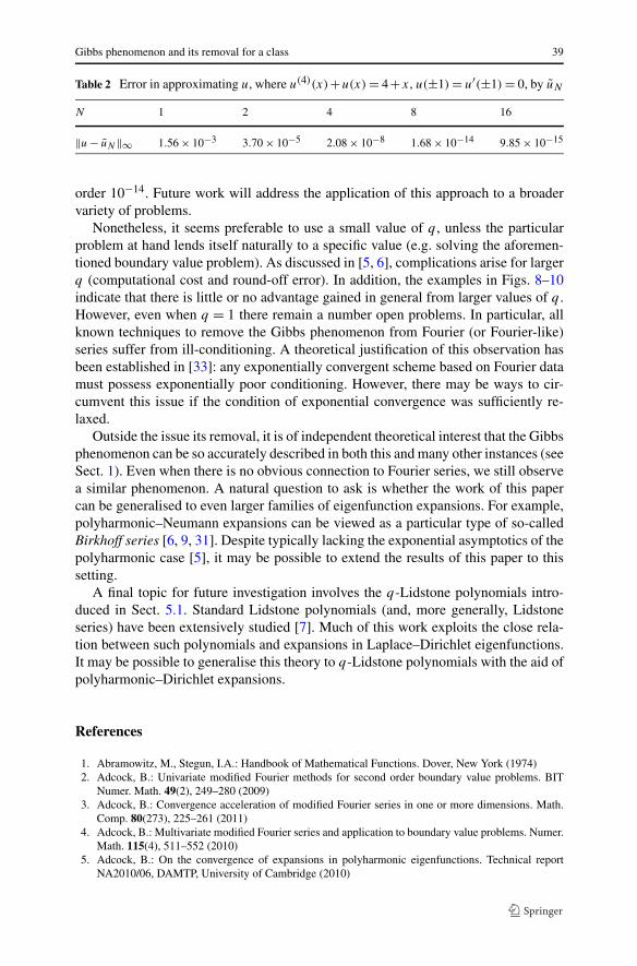
Gibbs phenomenon and its removal for a class 39
Table 2 Error in approximating u, where u(4)(x)+u(x) = 4+x, u(±1) = u′(±1) = 0, by uN
N 1 2 4 8 16
‖u − uN‖∞ 1.56 × 10⁻³ 3.70 × 10⁻⁵ 2.08 × 10⁻⁸ 1.68 × 10⁻¹⁴ 9.85 × 10⁻¹⁵
order 10−14. Future work will address the application of this approach to a broadervariety of problems.
Nonetheless, it seems preferable to use a small value of q , unless the particularproblem at hand lends itself naturally to a specific value (e.g. solving the aforemen-tioned boundary value problem). As discussed in [5, 6], complications arise for largerq (computational cost and round-off error). In addition, the examples in Figs. 8–10indicate that there is little or no advantage gained in general from larger values of q .However, even when q = 1 there remain a number open problems. In particular, allknown techniques to remove the Gibbs phenomenon from Fourier (or Fourier-like)series suffer from ill-conditioning. A theoretical justification of this observation hasbeen established in [33]: any exponentially convergent scheme based on Fourier datamust possess exponentially poor conditioning. However, there may be ways to cir-cumvent this issue if the condition of exponential convergence was sufficiently re-laxed.
Outside the issue its removal, it is of independent theoretical interest that the Gibbsphenomenon can be so accurately described in both this and many other instances (seeSect. 1). Even when there is no obvious connection to Fourier series, we still observea similar phenomenon. A natural question to ask is whether the work of this papercan be generalised to even larger families of eigenfunction expansions. For example,polyharmonic–Neumann expansions can be viewed as a particular type of so-calledBirkhoff series [6, 9, 31]. Despite typically lacking the exponential asymptotics of thepolyharmonic case [5], it may be possible to extend the results of this paper to thissetting.
A final topic for future investigation involves the q-Lidstone polynomials intro-duced in Sect. 5.1. Standard Lidstone polynomials (and, more generally, Lidstoneseries) have been extensively studied [7]. Much of this work exploits the close rela-tion between such polynomials and expansions in Laplace–Dirichlet eigenfunctions.It may be possible to generalise this theory to q-Lidstone polynomials with the aid ofpolyharmonic–Dirichlet expansions.
References
1. Abramowitz, M., Stegun, I.A.: Handbook of Mathematical Functions. Dover, New York (1974)2. Adcock, B.: Univariate modified Fourier methods for second order boundary value problems. BIT
Numer. Math. 49(2), 249–280 (2009)3. Adcock, B.: Convergence acceleration of modified Fourier series in one or more dimensions. Math.
Comp. 80(273), 225–261 (2011)4. Adcock, B.: Multivariate modified Fourier series and application to boundary value problems. Numer.
Math. 115(4), 511–552 (2010)5. Adcock, B.: On the convergence of expansions in polyharmonic eigenfunctions. Technical report
NA2010/06, DAMTP, University of Cambridge (2010)

40 B. Adcock
6. Adcock, B., Iserles, A., Nørsett, S.P.: From high oscillation to rapid approximation II: expansions inBirkhoff series. IMA J. Numer. Anal. (to appear) (2010)
7. Agarwal, R., Wong, P.: Error Inequalities in Polynomial Interpolation and Their Applications.Springer, Berlin (1993)
8. Baszenski, G., Delvos, F.J.: Accelerating the rate of convergence of bivariate Fourier expansions. In:Approximation Theory IV, pp. 335–340 (1983)
9. Birkhoff, G.D.: Boundary value and expansion problems of ordinary linear differential equations.Trans. Am. Math. Soc. 9(4), 373–395 (1908)
10. Boyd, J.P.: A comparison of numerical algorithms for Fourier extension of the first, second, and thirdkinds. J. Comput. Phys. 178, 118–160 (2002)
11. Boyd, J.P.: Acceleration of algebraically-converging Fourier series when the coefficients have seriesin powers of 1/n. J. Comput. Phys. 228, 1404–1411 (2009)
12. Brunner, H., Iserles, A., Nørsett, S.P.: The computation of the spectra of highly oscillatory Fredholmintegral operators. J. Integral Equ. Appl. (2010, to appear)
13. Driscoll, T.A., Fornberg, B.: A Padé-based algorithm for overcoming the Gibbs phenomenon. Numer.Algorithms 26, 77–92 (2001)
14. Eckhoff, K.S.: Accurate and efficient reconstruction of discontinuous functions from truncated seriesexpansions. Math. Comput. 61(204), 745–763 (1993)
15. Eckhoff, K.S.: Accurate reconstructions of functions of finite regularity from truncated Fourier seriesexpansions. Math. Comput. 64(210), 671–690 (1995)
16. Eckhoff, K.S.: On a high order numerical method for functions with singularities. Math. Comput.67(223), 1063–1087 (1998)
17. Fornberg, B., Flyer, N.: The Gibbs phenomenon for radial basis functions. In: Jerri, A. (ed.) The GibbsPhenomenon in Various Representations and Applications. Sampling Publishing, Potsdam (2007)
18. Gelb, A., Gottlieb, D.: The resolution of the Gibbs phenomenon for “spliced” functions in one andtwo dimensions. Comput. Math. Appl. 33(11), 35–58 (1997)
19. Gottlieb, D., Orszag, S.A.: Numerical Analysis of Spectral Methods: Theory and Applications, 1stedn. Society for Industrial and Applied Mathematics, Philadelphia (1977)
20. Gottlieb, D., Shu, C.W.: On the Gibbs’ phenomenon and its resolution. SIAM Rev. 39(4), 644–668(1997)
21. Gottlieb, D., Shu, C.W., Solomonoff, A., Vandeven, H.: On the Gibbs phenomenon I: recoveringexponential accuracy from the Fourier partial sum of a nonperiodic analytic function. J. Comput.Appl. Math. 43(1–2), 91–98 (1992)
22. Huybrechs, D.: On the Fourier extension of non-periodic functions. SIAM J. Numer. Anal. 47(6),4326–4355 (2010)
23. Iserles, A., Nørsett, S.P.: From high oscillation to rapid approximation I: modified Fourier expansions.IMA J. Numer. Anal. 28, 862–887 (2008)
24. Jerri, A.: The Gibbs Phenomenon in Fourier Analysis, Splines, and Wavelet Approximations.Springer, Berlin (1998)
25. Kantorovich, L.V., Krylov, V.I.: Approximate Methods of Higher Analysis, 3rd edn. Interscience,New York (1958)
26. Lorentz, G.G., Jetter, K., Riemenschneider, S.D.: Birkhoff Interpolation. Addison–Wesley, London(1983)
27. Lyness, J.N.: Adjusted forms of the Fourier coefficient asymptotic expansion and applications in nu-merical quadrature. Math. Comput. 25, 87–104 (1971)
28. Lyness, J.N.: Computational techniques based on the Lanczos representation. Math. Comput. 28(125),81–123 (1974)
29. Lyness, J.N.: The calculation of trigonometric Fourier coefficients. J. Comput. Phys. 54, 57–73 (1984)30. Minkin, A.M.: Equiconvergence theorems for differential operators. J. Math. Sci. 96, 3631–3715
(1999)31. Naimark, M.A.: Linear Differential Operators. Harrap, Bromley (1968)32. Olver, S.: On the convergence rate of a modified Fourier series. Math. Comput. 78, 1629–1645 (2009)33. Platte, R., Trefethen, L.N., Kuijlaars, A.: Impossibility of fast stable approximation of analytic func-
tions from equispaced samples. SIAM Rev. (2010, to appear)34. Shaw, J.K., Johnson, L.W., Riess, R.D.: Accelerating convergence of eigenfunction expansions. Math.
Comput. 30(135), 469–477 (1976)35. Sidi, A.: Practical Extrapolation Methods. Theory and Applications. Cambridge Monographs on Ap-
plied and Computational Mathematics, vol. 10. Cambridge University Press, Cambridge (2003)

Gibbs phenomenon and its removal for a class 41
36. Smitheman, S.A., Spence, E.A., Fokas, A.S.: A spectral collocation method for the Laplace and mod-ified Helmholtz equations in a convex polygon. IMA J. Numer. Anal. 30(4), 1184–1205 (2010)
37. Srivastava, H., Choi, J.: Series Associated with the Zeta and Related Functions. Kluwer Academic,Dordrecht (2001)
38. Tadmor, E.: Filters, mollifiers and the computation of the Gibbs’ phenomenon. Acta Numer. 16, 305–378 (2007)
39. Young, R.M.: An Introduction to Nonharmonic Fourier Series, 1st edn. Academic Press, San Diego(2001)
40. Zygmund, A.: Trigonometric Series, vol. 1. Cambridge University Press, Cambridge (1959)