orthogonal polynomial expansions for - college of

International Journal for Uncertainty Quantification,1 (2): 163–187 (2011)

ORTHOGONAL POLYNOMIAL EXPANSIONS FORSOLVING RANDOM EIGENVALUE PROBLEMS

Sharif Rahman∗ & Vaibhav Yadav

College of Engineering and Program of Applied Mathematical and Computational Sciences, TheUniversity of Iowa, Iowa City, IA 52242

Original Manuscript Submitted: 03/08/2010; Final Draft Received: 12/12/2010

This paper examines two stochastic methods stemming from polynomial dimensional decomposition (PDD) and polyno-mial chaos expansion (PCE) for solving random eigenvalue problems commonly encountered in dynamics of mechanicalsystems. Although the infinite series from PCE and PDD are equivalent, their truncations endow contrasting dimen-sional structures, creating significant differences between the resulting PDD and PCE approximations in terms ofaccuracy, efficiency, and convergence properties. When the cooperative effects of input variables on an eigenvalue atten-uate rapidly or vanish altogether, the PDD approximation commits a smaller error than does the PCE approximation foridentical expansion orders. Numerical analyses of mathematical functions or simple dynamic systems reveal markedlyhigher convergence rates of the PDD approximation than the PCE approximation. From the comparison of computa-tional efforts, required to estimate with the same precision the frequency distributions of dynamic systems, including apiezoelectric transducer, the PDD approximation is significantly more efficient than the PCE approximation.

KEY WORDS: stochastic mechanics, random matrix, polynomial dimensional decomposition, polynomialchaos expansion, piezoelectric transducer

1. INTRODUCTION

Random eigenvalue problems (REPs) comprising stochastic matrix, differential, or integral operators frequently ap-pear in many fields of engineering, science, and mathematics. They are commonly solved by stochastic methods thatdetermine the statistical moments, probability law, and other relevant properties of eigensolutions. The solutions mayrepresent oscillatory modes of a mechanical or structural system (e.g., vehicles, buildings, bridges), disposition ofelectrons around an atom or a molecule, acoustic modes of a concert hall, eigenfaces in computer vision technology,spectral properties of a graph, and numerous other physical or mathematical quantities.

Many REPs are focused on the second-moment properties of eigensolutions, for which there exist a multitude ofmethods or approaches. Prominent among them are the classical perturbation method [1], the iteration method [1], theRitz method [2], the crossing theory [3], the stochastic reduced basis approach [4], and the asymptotic method [5].More recent developments on solving REPs include the stochastic expansion methods, notably, the polynomial chaosexpansion (PCE) [6] and polynomial dimensional decomposition (PDD) [7] methods, both employing Fourier expan-sions in terms of orthogonal polynomials for approximating eigensolutions. The latter two methods also provide theprobability distributions of eigensolutions, although the concomitant approximations are guaranteed to converge onlyin the mean-square sense, provided that the eigensolutions are square-integrable functions of the random input withrespect to its probability measure. A distinguishing feature of these expansion methods is their effective exploitation ofthe smoothness properties of eigensolutions, if they exist, with the attendant convergence rates markedly higher thanthose obtained from the sampling-based methods. However, due to the contrasting dimensional structures of PDDand PCE, the convergence properties of their truncations are not the same and may differ significantly, dependingon the eigensolution and dimension of the problem. Therefore, uncovering their mathematical properties, which have

∗Correspond to Sharif Rahman, E-mail: [email protected]

2152–5080/11/$35.00 c© 2011 by Begell House, Inc. 163

Begell House Digital Library, http://dl.begellhouse.com Downloaded 2011-2-28 from IP 128.255.19.140 by

164 Rahman & Yadav

ramifications in stochastic computing, including solving REPs, is a major motivation for this current work. Is PDDsuperior to PCE or vice versa? It is also desirable to compare the errors from the PDD and PCE approximations andthereby establish appropriate criteria for grading these two methods.

This paper presents a rigorous comparison of the PDD and PCE methods for calculating the statistical momentsand tail probability distributions of random eigenvalues commonly encountered in dynamics of mechanical systems.The methods are based on (i) a broad range of orthonormal polynomial bases consistent with the probability measureof the random input and (ii) an innovative dimension-reduction integration for calculating the expansion coefficients.Section 2 formally defines the REP addressed in this study. Section 3 provides a brief exposition of PDD and PCE,including establishing the relationship between the two expansions. Section 4 discusses PDD and PCE approxima-tions resulting from series truncations, where an alternative form of the PCE approximation has been derived, leadingto approximate probabilistic solutions from both methods in terms of the PDD expansion coefficients. Section 4 alsopresents an error analysis due to PDD and PCE approximations. Section 5 describes the dimension-reduction inte-gration for estimating the PDD expansion coefficients, including the computational efforts required. Five numericalexamples illustrate the accuracy, convergence, and computational efficiency of the PDD and PCE methods in Sec-tion 6. Finally, conclusions are drawn in Section 7.

2. EIGENVALUE PROBLEMS IN STOCHASTIC DYNAMICS

Let (Ω,F , P ) be a complete probability space, whereΩ is a sample space,F is aσ-field onΩ, andP : F → [0, 1] isa probability measure. LetRN andCN beN -dimensional real and complex vectors spaces, respectively, andRN×N

a set of allN × N , real-valued matrices. WithBN representing a Borelσ-field onRN andE the expectation oper-ator on(Ω,F , P ), consider anRN -valued, independent, input random vectorX = X1, . . . , XNT : (Ω,F) →(RN ,BN ), which has mean vectorµX := E[X] ∈ RN , covariance matrixΣX := E[(X − µX)(X − µX)T ] ∈RN×N , and joint probability density functionfX(x) = Πi=N

i=1 fi(xi), wherefi(xi) is the marginal probability densityfunction ofXi defined on the probability triple(Ωi,Fi, Pi). In most dynamic systems, the vectorX represents uncer-tainties in material parameters (e.g., mass, damping, stiffness), geometry (e.g., size, shape, topology), and constraints(e.g., initial and boundary conditions).

Consider a family ofL×L, real-valued, random coefficient matricesAj(X) ∈ RL×L, j = 1, . . . , J , whereJ isa positive integer and a general nonlinear functionf . The probabilistic characteristics ofAj(X) can be derived fromthe known probability law ofX. A nontrivial solution of

f [λ(X); A1(X), . . . , AJ(X)] φ(X) = 0, (1)

if it exists, defines the random eigenvalueλ(X) ∈ R or C and the random eigenvectorφ(X) ∈ RL or CL of ageneral nonlinear eigenvalue problem. Depending on the type of application, a wide variety of functionsf and, hence,eigenvalue problems exist. Table 1 shows a few examples of REPs frequently encountered in dynamic systems. Ingeneral, the eigensolutions depend on the random inputX via solution of the matrix characteristic equation

det f [λ(X); A1(X), . . . , AJ(X)] = 0 (2)

and subsequent solution of Eq. (1). A major objective in solving a random eigenvalue problem is to find the proba-bilistic characteristics of eigenpairsλ(i)(X),φ(i)(X), i = 1, . . . , L, when the probability law ofX is arbitrarilyprescribed. Both the PDD and PCE methods can be employed to solve any REP in Table 1, however, yielding differ-ent accuracy or efficiency with significant implications in stochastic computing. Therefore, a rigorous comparison ofthese two expansion methods—the principal focus of this work—should provide deeper insights into their respectivecapabilities as well as limitations.

3. STOCHASTIC EIGENVALUE EXPANSIONS

Let λ(X), a real-valued, mean-square integrable, measurable transformation on(Ω,F), define a relevant eigenvalueof a stochastic dynamic system. In general, the multivariate functionλ : RN → R is implicit, is not analytically

International Journal for Uncertainty Quantification


Solving Random Eigenvalue Problems 165

TABLE 1: Random eigenvalue problems in stochastic dynamical systems

Eigenvalue problem(a) Problem type and application(s)

[−λ(X)M(X) + K(X)] φ(X) = 0Linear: undamped or proportionallydamped systems

[λ2(X)M(X) + λ(X)C(X) + K(X)

]φ(X) = 0

Quadratic:non-proportionally dampedsystems, singularity problems

[λ(X)M1(X) + M0(X) + MT

1 (X)/λ(X)]φ(X) = 0

Palindromic: acoustic emissions inhigh-speed trains[∑

k

λk(X)Ak(X)

]φ(X) = 0

Polynomial: control and dynamicsproblems

[λ(X)M(X)−K(X) +

∑

k

λq(X)Ck(X)ak − λ(X)

]φ(X) = 0

Rational: plate vibration(q = 1), fluid-structure vibration(q = 2), vibration ofviscoelastic materials

(a)M(X), C(X), and K(X) are mass, damping, stiffness matrices, respectively;M0(X), M1(X),Ak(X), andCk(X) are various coefficient matrices.

available, and can only be viewed as a high-dimensional input-output mapping, where the evaluation of the outputfunction λ for a given inputX requires expensive finite element analysis (FEA). Therefore, methods employed instochastic analysis must be capable of generating accurate probabilistic characteristics ofλ(X) with an acceptablysmall number of output function evaluations.

3.1 Orthonormal Polynomials

LetL2(Ωi,Fi, Pi) be a Hilbert space that is equipped with a set of complete orthonormal basesψij(xi); j = 0, 1, . . .,which is consistent with the probability measure ofXi. For example, classical orthonormal polynomials, includ-ing Hermite, Legendre, and Jacobi polynomials, can be used whenXi follows Gaussian, uniform, andβ probabil-ity distributions, respectively [8]. For an arbitrary measure, approximate methods based on the Stieltjes procedurecan be employed to obtain the associated orthonormal polynomials [8, 9]. IfE is the expectation operator with re-spect to the probability measure ofX, then two important properties of orthonormal polynomials are as follows[9, 10].Property 1. The orthonormal polynomial basis functions have a unit mean forj = 0 and zero means for allj ≥ 1,i.e.,

E[ψij(Xi)] :=∫

Rψij(xi)fi(xi)dxi =

1 if j = 0,

0 if j ≥ 1.(3)

Property 2. Any two orthonormal polynomial basis functionsψij1(Xi) andψij2(Xi), wherej1, j2 = 0, 1, 2, . . ., areuncorrelated and each has unit variance, i.e.,

E[ψij1(Xi)ψij2(Xi)] :=∫

Rψij1(xi)ψij2(xi)fi(xi)dxi =

1 if j1 = j2,

0 if j1 6= j2.(4)

If λ is a sufficiently smooth function ofX, then there exist two important stochastic expansions of random eigenvaluesinvolving orthonormal polynomials, as follows.

3.2 Polynomial dimensional decomposition

The PDD of a random eigenvalueλ(X) represents a finite, hierarchical expansion [7, 9]

Volume 1, Number 2, 2011


166 Rahman & Yadav

λPDD(X) := λ0 +N∑

i=1

∞∑

j=1

Cijψij(Xi) +N−1∑

i1=1

N∑

i2=i1+1

∞∑

j2=1

∞∑

j1=1

Ci1i2j1j2ψi1j1(Xi1)ψi2j2(Xi2)

+N−2∑

i1=1

N−1∑

i2=i1+1

N∑

i3=i2+1

∞∑

j3=1

∞∑

j2=1

∞∑

j1=1

Ci1i2i3j1j2j3ψi1j1(Xi1)ψi2j2(Xi2)ψi3j3(Xi3)

+ . . . +1∑

i1=1

. . .

N∑

iN=iN−1+1

∞∑

jN=1

. . .

∞∑

j1=1

Ci1...iN j1...jN

N∏q=1

ψiqjq (Xiq )

= λ0 +N∑

s=1

[N−s+1∑

i1=1

. . .

N∑

is=is−1+1︸︷︷︸s sums

∞∑

j1=1

. . .

∞∑

js=1︸︷︷︸s sums

Ci1...isj1...js

s∏q=1

ψiqjq(Xiq

)

]

(5)

in terms of random orthonormal polynomialsψij(Xi), i = 1, . . . , N ; j = 1, . . . ,∞ of input variablesX1, . . . , XN

with increasing dimensions, where

λ0 :=∫

RN

λ(x)fX(x)dx (6)

and

Ci1...isj1...js :=∫

RN

λ(x)s∏

q=1

ψiqjq (xiq )fX(x)dx, (7)

for s = 1, ..., N, 1≤ i1 < ... < is ≤N , j1, ..., js = 1, ...,∞ are the associated expansion coefficients, which requirecalculating various high-dimensional integrals whenN is large. In Eq. (5), the term

∑∞js=1...

∑∞j1=1Ci1...isj1...js

∏sq=1

ψiqjq (Xiq ) represents thes-variate component function, quantifying the cooperative effect ofs input variablesXi1 , ...,XiS

onλ.

3.3 Polynomial Chaos Expansion

The PCE of a random eigenvalueλ(X), a function of a finite number of random variablesX1, . . . , XN , has a repre-sentation [11–13]

λPCE(X) := a0Γ0 +N∑

i=1

aiΓ1(Xi) +N∑

i1=1

N∑

i2=i1

ai1i2Γ2(Xi1 , Xi2) +N∑

i1=1

N∑

i2=i1

N∑

i3=i2

ai1i2i3Γ3(Xi1 , Xi2 , Xi3)

+ . . . +N∑

i1=1

. . .

N∑

ip=ip−1

ai1...ipΓp(Xi1 , . . . , Xip) + . . .

(8)

in terms of random polynomial chaoses,Γp(Xi1 , . . . , Xip), p = 0, . . . ,∞, 1 ≤ i1 ≤ . . . ≤ ip ≤ N , of input variablesXi1 , . . . , Xip with increasing orders, where

a0 :=∫

RN

λ(x)Γ0fX(x)dx (9)

and

ai1...ip :=∫

RN

λ(x)Γp(Xi1 , . . . , Xip)fX(x)dx, (10)

for p = 1, . . . ,∞, 1 ≤ i1 ≤ . . . ≤ ip ≤ N , are the corresponding expansion coefficients that also require evaluatinghigh-dimensional integrals.




Once the expansion coefficients in Eq. (5) or (8) are determined, as explained in a forthcoming section, PDD andPCE furnish surrogates of the exact mapλ : RN → R, describing an input-output relationship from a complicatednumerical eigenvalue analysis. Therefore, any probabilistic characteristic ofλ(X), including its statistical momentsand rare event probabilities, can be estimated from its PDD or PCE.

Remark 1.Using Properties 1 and 2 of orthonormal polynomials, it is elementary to show that the second-momentproperties of any mean-square integrable functionλ(X), its PDDλPDD(X), and its PCEλPCE(X) are identical. Inother words,λ(X), λPDD(X), andλPCE(X) are equivalent in the mean-square sense.

3.4 Relationship between PDD and PCE

Because the polynomial chaoses in Eq. (8) are built from univariate orthonormal polynomials, PDD and PCE arerelated. Indeed, there exists a striking theorem, as follows.

Theorem 1.If λPDD(X) andλPCE(X) are two infinite series defined in Eqs. (5) and (8), respectively, then oneseries can be rearranged to derive the other series, for instance,λPCE(X) = λPDD(X).

Proof. The polynomial chaosesΓp(Xi1 , . . . , Xip), p = 0, . . . ,∞, 1 ≤ i1 ≤ . . . ≤ ip ≤ N in Eq. (8) can be moreexplicitly written as

Γ0 = 1

Γ1(Xi) = ψi1(Xi)

Γ2(Xi1 , Xi2) = ψi12(Xi1)δi1i2 −ψi11(Xi1)ψi21(Xi2)(δi1i2 − 1)

Γ3(Xi1 , Xi2 , Xi3) = ψi13(Xi1)δi1i2δi1i3δi2i3

− ψi11(Xi1)ψi22(Xi2)δi2i3(δi1i2 − 1)

− ψi22(Xi2)ψi31(Xi3)δi1i2(δi2i3 − 1)

− ψi11(Xi1)ψi21(Xi2)ψi31(Xi3)(δi1i2δi1i3δi2i3 − 1)(δi1i2 − 1)(δi2i3 − 1). . . = . . . ,

(11)

which represents various combinations of tensor products of sets of univariate orthonormal polynomials withδikil,

k, l = 1, . . . , p, denoting various Kronecker deltas, i.e.,δikil= 1 whenik = il and zero otherwise. Inserting Eq. (11)

into Eqs. (9) and (10) with Eqs. (6) and (7) in mind, the PCE coefficients,

a0 = λ0

ai = Ci1

ai1i2 = Ci12δi1i2 − Ci1i211(δi1i2 − 1)

ai1i2i3 = Ci13δi1i2δi1i3δi2i3 − Ci1i212δi2i3(δi1i2 − 1)

− Ci2i321δi1i2(δi2i3 − 1)

− Ci1i2i3111(δi1i2δi1i3δi2i3 − 1)(δi1i2 − 1)(δi2i3 − 1). . . = . . . ,

(12)

provide explicit connections to the PDD coefficients. Using the polynomial chaoses and PCE coefficients fromEqs. (11) and (12), respectively, and after some simplifications, the zero- to higher-order PCE terms become



168 Rahman & Yadav

a0Γ0 = λ0N∑

i=1

aiΓ1(Xi) =N∑

i=1

Ci1ψi1(Xi)

N∑

i1=1

N∑

i2=i1

ai1i2Γ2(Xi1 , Xi2) =N∑

i=1

Ci2ψi2(Xi) +N∑

i1,i2=1;i1<i2

Ci1i211ψi11(Xi1)ψi21(Xi2)

N∑

i1=1

N∑

i2=i1

N∑

i3=i2

ai1i2i3Γ3(Xi1 , Xi2 , Xi3) =N∑

i=1

Ci3ψi3(Xi) +N∑

i1,i2=1;i1<i2


+N∑

i1,i2=1;i1<i2


+N∑

i1,i2,i3=1;i1<i2<i3

Ci1i2i3111ψi11(Xi1)ψi21(Xi2)ψi31(Xi3)

. . . = . . . ,

(13)

revealing constituents comprising constant, univariate functions, bivariate functions, etc. Collecting all univariateterms, all bivariate terms, etc., from each appropriate line of Eq. (13) leads to

λPCE(X) = limp→∞

[λ0 +

N∑

i=1

p∑

j=1


i1=1

N∑

i2=i1+1

p−1∑

j2=1

p−1∑

j1=1︸︷︷︸j1+j2≤p


+N−2∑

i1=1

N−1∑

i2=i1+1

N∑

i3=i2+1

p−2∑

j3=1

p−2∑

j2=1

p−2∑

j1=1︸︷︷︸j1+j2+j3≤p


+ . . . +1∑

i1=1

. . .

N∑

iN=iN−1+1

p−N+1∑

jN=1

. . .

p−N+1∑

j1=1︸︷︷︸j1+...+jN≤p

Ci1...iN j1...jN

N∏q=1

ψiqjq (Xiq )

]

= λ0 +N∑

i=1

∞∑

j=1


i1=1

N∑

i2=i1+1

∞∑

j2=1

∞∑

j1=1


+N−2∑

i1=1

N−1∑

i2=i1+1

N∑

i3=i2+1

∞∑

j3=1

∞∑

j2=1

∞∑

j1=1


+ . . . +1∑

i1=1

. . .

N∑

iN=iN−1+1

∞∑

jN=1

. . .

∞∑

j1=1

Ci1...iN j1...jN

N∏q=1

ψiqjq (Xiq )

= λ0 +N∑

s=1

[N−s+1∑

i1=1

. . .

N∑


∞∑

j1=1

. . .

∞∑


Ci1...isj1...js

s∏q=1

ψiqjq (Xiq )

]=: λPDD(X),

(14)which proves the theorem for any mean-square integrable functionλ : RN → R, 1 ≤ N < ∞, and probabilitydistribution ofX.




4. SERIES TRUNCATIONS AND APPROXIMATE SOLUTIONS

4.1 PDD Approximation

Although Eq. (5) provides an exact PDD representation, it contains an infinite number of coefficients, emanating frominfinite numbers of orthonormal polynomials. In practice, the number of coefficients must be finite, say, by retaining atmostmth-order polynomials in each variable. Furthermore, in many applications, the functionλ can be approximatedby a sum of at mostS-variate component functions, where1 ≤ S ≤ N is another truncation parameter, resulting intheS-variate,mth-order PDD approximation

λS,m(X) = λ0 +S∑

s=1

[N−s+1∑

i1=1

. . .

N∑


m∑

j1=1

. . .

m∑


Ci1...isj1...js

s∏q=1

ψiqjq(Xiq

)

], (15)

containing

QS,m =S∑

k=0

(N

S − k

)mS−k (16)

number of PDD coefficients and corresponding orthonormal polynomials. The PDD approximation in Eq. (15) in-cludes cooperative effects of at mostS input variablesXi1 , . . . , XiS

, 1 ≤ i1 ≤ . . . ≤ iS ≤ N , onλ. For instance, byselectingS = 1 and2, the functions,λ1,m(X) andλ2,m(X), respectively, provide univariate and bivariatemth-orderapproximations, contain contributions from all input variables, and should not be viewed as first- and second-orderapproximations, nor do they limit the nonlinearity ofλ(X). Depending on how the component functions are con-structed, arbitrarily high-order univariate and bivariate terms ofλ(X) could be lurking insideλ1,m(X) andλ2,m(X).The fundamental conjecture underlying this decomposition is that the component functions arising in the functiondecomposition will exhibit insignificantS-variate effects cooperatively whenS → N , leading to useful lower-variateapproximations ofλ(X). WhenS → N andm → ∞, λS,m(X) converges toλ(X) in the mean-square sense, i.e.,Eq. (15) generates a hierarchical and convergent sequence of approximations ofλ(X).

Applying the expectation operator on Eq. (15) and noting property 1, the meanE[λS,m(X)

]= λ0 of the S-

variate,mth-order approximation of the eigenvalue matches the exact mean of the eigenvalue in Eq. (6), regardless of

S or m. Applying the expectation operator again, this time on[λS,m(X)− λ0

]2

, results in the approximate variance

E[λS,m(X)−λ0

]2

=S∑

s=1

S∑t=1

(N−s+1∑

i1=1

...

N∑

is=is−1+1

m∑

j1=1

...

m∑

js=1︸︷︷︸2s sums

N−t+1∑

k1=1

...

N∑

kt=kt−1+1

m∑

l1=1

...

m∑

lt=1︸︷︷︸2t sums

Ci1...isj1...js

× Ck1...ktl1...ltE

[s∏

q=1

ψiqjq (Xiq )t∏

q=1

ψkqlq (Xkq )

]) (17)

of the eigenvalue, which depends onS andm. The number of summations inside the parenthesis of the right side ofEq. (17) is2(s+t), wheres andt are the indices of the two outer summations. By virtue of property 2 and independentcoordinates ofX,

E

[s∏

q=1

ψiqjq (Xiq )t∏

q=1

ψkqlq (Xkq )

]=

s∏q=1

E[ψ2

iqjq(Xiq )

]= 1 (18)

for s = t, iq = kq, jq = lq and zero otherwise, leading to



170 Rahman & Yadav

E[λS,m(X)− λ0

]2

=S∑

s=1

(N−s+1∑

i1=1

. . .

N∑


m∑

j1=1

. . .

m∑


C2i1...isj1...js

)(19)

as the sum of squares of the expansion coefficients from theS-variate,mth-order PDD approximation ofλ(X).Clearly, the approximate variance in Eq. (19) approaches the exact variance

E [λ(X)− λ0]2 = E [λPDD(X)− λ0]

2 =N∑

s=1

(N−(s+1)∑

i1=1

. . .

N∑


∞∑

j1=1

. . .

∞∑


C2i1...isj1...js

)

(20)

of the eigenvalue whenS → N andm → ∞. The mean-square convergence ofλS,m is guaranteed asλ and itscomponent functions are all members of the associated Hilbert spaces.

Remark 2. The expansion orderm, which is a positive integer, should be interpreted as the largest exponent of asingle variable from the monomials (terms) of the PDD approximation. On the basis of the traditional definition, thetotal order of the multivariate polynomial in the right side of Eq. (15) isSm, although all monomials with total degreeequal to or less thanSm are not present.

4.2 PCE Approximation

Thepth-order PCE approximation

λp(X) := a0Γ0 +N∑

i=1

aiΓ1(Xi) +N∑

i1=1

N∑

i2=i1

ai1i2Γ2(Xi1 , Xi2) +N∑

i1=1

N∑

i2=i1

N∑

i3=i2

ai1i2i3Γ3(Xi1 , Xi2 , Xi3)

+ . . . +N∑

i1=1

. . .

N∑

ip=ip−1

ai1...ipΓp(Xi1 , . . . , Xip),

(21)

obtained directly by truncating the right side of Eq. (8), requires(N + p)!/(N !p!) number of the PCE coefficients.However, since PDD and PCE are related, the terms of Eq. (21) can be rearranged following similar derivations inproving Theorem 1, resulting in

λp(X) = λ0 +N∑

i=1

p∑

j=1


i1=1

N∑

i2=i1+1

p−1∑

j2=1

p−1∑

j1=1︸︷︷︸j1+j2≤p


+N−2∑

i1=1

N−1∑

i2=i1+1

N∑

i3=i2+1

p−2∑

j3=1

p−2∑

j2=1

p−2∑

j1=1︸︷︷︸j1+j2+j3≤p


+ . . . +N−s+1∑

i1=1

. . .

N∑

is=is−1+1

p−N+1∑

jN=1

. . .

p−N+1∑

j1=1︸︷︷︸j1+...+jN≤p

Ci1...iN j1...jN

N∏q=1

ψiqjq (Xiq )

(22)

with the generic(s + 1)th term,s = 1, . . . , p, shown or its abbreviated form

λp(X) = λ0 +N∑

s=1

[N−s+1∑

i1=1

. . .

N∑


p−s+1∑

j1=1

. . .

p−s+1∑

js=1︸︷︷︸s sums;j1+...+js≤p

Ci1...isj1...js

s∏q=1

ψiqjq (Xiq )

], (23)




involving solely

Qp =N∑

k=0

(N

N − k

)(p

N − k

)(24)

number of PDD coefficients and corresponding orthonormal polynomials, where(

pN−k

)should be interpreted as zero

whenp < N −k. It is elementary to show thatQp matches(N + p)!/(N !p!), the original number of PCE coefficientsfrom Eq. (21). The advantage of Eq. (23) over Eq. (21) is that the PDD coefficients, once determined, can be reusedfor the PCE approximation, thereby sidestepping calculations of the PCE coefficients.

Applying the expectation operator on Eq. (23) and noting Property 1, the meanE[λp(X)

]= λ0 of thepth-order

PCE approximation of the eigenvalue also matches the exact mean of the eigenvalue for any expansion order. Applyingthe expectation operator on

[λp(X)− λ0

]2and following similar arguments as before, the variance of thepth-order

PCE approximation of the eigenvalue is

E[λp(X)− λ0

]2 =N∑

s=1

(N−s+1∑

i1=1

. . .

N∑


p−s+1∑

j1=1

. . .

p−s+1∑

js=1︸︷︷︸s sums;j1+...+js≤p

C2i1...isj1...js

), (25)

another sum of squares of the PDD expansion coefficients such thatj1 + . . . + js ≤ p, which also converges toE [λ(X)− λ0]

2 asp →∞.Remark 3. Two important observations can be made when comparing the PDD and PCE approximations ex-

pressed by Eqs. (15) and (21), respectively. First, the terms in the PCE approximation are organized with respect tothe order of polynomials. In contrast, the PDD approximation is structured with respect to the degree of cooperativitybetween a finite number of random variables. Therefore, significant differences may exist regarding the accuracy,efficiency, and convergence properties of their truncated sum or series. Second, if an eigenvalue response is highlynonlinear but contains rapidly diminishing cooperative effects of multiple random variables, the PDD approximationis expected to be more effective than the PCE approximation. This is because the lower-variate (univariate, bivariate,etc.) terms of the PDD approximation can be just as nonlinear by selecting appropriate values ofm in Eq. (15). Incontrast, many more terms and expansion coefficients are required to be included in the PCE approximation to capturesuch high nonlinearity.

Remark 4.Depending on the problem size (N ) and truncation parameters (S, m, p), there exist a few special caseswhere the PDD and PCE approximations coincide: (i) whenN = 1, the univariate,mth-order PDD andmth-orderPCE approximations are the same, i.e.,λ1,m(X) = λm(X) for any1 ≤ m < ∞; (ii) for any arbitrary value ofN , theunivariate, first-order PDD and first-order PCE approximations are the same, i.e.,λ1,1(X) = λ1(X).

Remark 5. The PDD and PCE approximations, regardless of the truncation parameters, predict the exact meanof an eigenvalue. However, the calculated variances of an eigenvalue from Eqs. (19) and (25) forS < N , m < ∞,andp < ∞ are neither the same nor exact, in general. Therefore, an error analysis, at least pertaining to the second-moment properties of eigensolutions, is required for comparing the PDD and PCE approximations.

4.3 Error Analysis

Define two errors,

eS,m := E[λ(X)− λS,m(X)

]2

= E[λPDD(X)− λS,m(X)

]2

=∫RN

[λPDD(x)− λS,m(x)

]2

fX(x)dx(26)

andep := E

[λ(X)− λp(X)

]2 = E[λPDD(X)− λp(X)

]2=

∫RN

[λPDD(x)− λp(x)

]2fX(x)dx,

(27)



172 Rahman & Yadav

owing toS-variate,mth-order PDD approximationλS,m(X) andpth-order PCE approximationλp(X), respectively,of λ(X). ReplacingλPDD, λS,m, andλp in Eqs. (26) and (27) with the right sides of Eqs. (5), (15), and (23), respec-tively, and invoking properties 1 and 2 yields the PDD error

eS,m =S∑

s=1

(N−s+1∑

i1=1

. . .

N∑


∞∑

j1=m+1

. . .

∞∑

js=m+1︸︷︷︸s sums

C2i1...isj1...js

)

+N∑

s=S+1

(N−s+1∑

i1=1

. . .

N∑


∞∑

j1=1

. . .

∞∑


C2i1...isj1...js

) (28)

and the PCE error

ep =N∑

s=1

(N−s+1∑

i1=1

. . .

N∑


∞∑

j1=1

. . .

∞∑

js=1︸︷︷︸s sums;j1+...+js>p

C2i1...isj1...js

), (29)

both consisting of the eliminated PDD coefficients as a result of truncations. In Eq. (28), the first term of the PDD erroris due to the truncations of polynomial expansion orders involving main and cooperative effects of at mostS variables,whereas the second term of the PDD error is contributed by ignoring the cooperative effects of larger thanS variables.In contrast, the PCE error in Eq. (29) derives from the truncations of polynomial expansion orders involving all mainand cooperative effects. By selecting1 ≤ S ≤ N , 1 ≤ m < ∞, and1 ≤ p < ∞, the errors can be determined forany PDD and PCE approximations, provided that all coefficients required by Eqs. (28) and (29) can be calculated.

For a general REP, comparing the PDD and PCE errors theoretically based on Eqs. (28) and (29) is not sim-ple, because it depends on which expansion coefficients decay and how they decay with respect to the truncationparametersS, m, andp. However, for a class of problems where the cooperative effects ofS input variables on aneigenvalue get progressively weaker asS → N , then the PDD and PCE errors for identical expansion orders can beweighed against each other. For this special case,m = p, assume thatCi1...isj1...js = 0, wheres = S + 1, . . . , N ,1 ≤ i1 < . . . < is ≤ N , j1, . . . , js = 1, . . . ,∞, for both the PDD and PCE approximations. Then, the second termon the right side of Eq. (28) vanishes, resulting in the PDD error

eS,m =S∑

s=1

(N−s+1∑

i1=1

. . .

N∑


∞∑

j1=m+1

. . .

∞∑

js=m+1︸︷︷︸s sums

C2i1...isj1...js

)

=S∑

s=1

(N−s+1∑

i1=1

. . .

N∑


∞∑

j1=1

. . .

∞∑


C2i1...isj1...js

)

−S∑

s=1

(N−s+1∑

i1=1

. . .

N∑


m∑

j1=1

. . .

m∑


C2i1...isj1...js

),

(30)

while the PCE error can be split into




em =S∑

s=1

(N−s+1∑

i1=1

. . .

N∑


∞∑

j1=1

. . .

∞∑


C2i1...isj1...js

)

−S∑

s=1

(N−s+1∑

i1=1

. . .

N∑


m−s+1∑

j1=1

. . .

m−s+1∑

js=1︸︷︷︸s sums;j1+...+js≤m

C2i1...isj1...js

)

≥S∑

s=1

(N−s+1∑

i1=1

. . .

N∑


∞∑

j1=1

. . .

∞∑


C2i1...isj1...js

)

−S∑

s=1

(N−s+1∑

i1=1

. . .

N∑


m∑

j1=1

. . .

m∑


C2i1...isj1...js

)= eS,m,

(31)

demonstrating larger error from the PCE approximation than from the PDD approximation. In the limit, whenS = N ,similar derivations showem ≥ eN,m, regardless of the values of the expansions coefficients. In other words, theN -variate,mth-order PDD approximation cannot be worse than themth-order PCE approximation. WhenS < N andCi1...isj1...js , s = S + 1, . . . , N , 1 ≤ i1 < . . . < is ≤ N , j1, . . . , js = 1, . . . ,∞, are not negligible and arbitrary,numerical convergence analysis is required for comparing these two errors.

Remark 6. The stochastic and error analyses aimed at higher-order moments or probability distribution ofλ canbe envisioned, but no closed-form solutions or simple expressions are possible. However, ifλ is sufficiently smoothwith respect toX—a condition fulfilled by many realistic eigenvalue problems—then Monte Carlo simulation of boththe PDD and PCE approximations can be efficiently conducted for also estimating the tail probabilistic characteristicsof eigensolutions.

5. CALCULATION OF EXPANSION COEFFICIENTS

The determination of the expansion coefficients required by the PDD or PCE approximation involves variousN -dimensional integrals overRN and is computationally prohibitive to evaluate whenN is arbitrarily large. Instead, adimension-reduction integration, presented as follows, was applied to estimate the coefficients efficiently [14].

5.1 Dimension-Reduction Integration

Letc = c1, . . . , cNT be a reference point of inputX andλ(c1, . . . , ci1−1, Xi1 , ci1+1, . . . , ciR−k−1, XiR−k, ciR−k+1,

. . . , cN ) represent an(R − k)th dimensional component function ofλ(X), where1 ≤ R < N is an integer,k = 0, . . . , R, and1 ≤ i1 < . . . < iR−k ≤ N . For example, whenR = 1, the zero-dimensional component function,which is a constant, isλ(c) and the one-dimensional component functions areλ(X1, c2, . . . , cN ), λ(c1, X2, . . . , cN ),. . ., λ(c1, c2, . . . , XN ). Using Xu and Rahman’s multivariate function theorem [15], it can be shown that theR-variateapproximation ofλ(X), defined by

λR(X) :=R∑

k=0

(−1)k

(N −R + k − 1

k

)

×N−R+k+1∑

i1=1

...

N∑

iR−k=iR−k−1+1︸︷︷︸(R−k) sums

y(c1, ..., ci1−1, Xi1 , ci1+1, ..., ciR−k−1, XiR−k, ciR−k+1, ..., cN ), (32)



174 Rahman & Yadav

consists of all terms of the Taylor series ofλ(X) that have less than or equal toR variables. The expanded form ofEq. (32), when compared with the Taylor expansion ofλ(X), indicates that the residual error inλR(X) includes termsof dimensionsR +1 and higher. All higher-orderR- and lower-variate terms ofλ(X) are included in Eq. (32), whichshould therefore generally provide a higher-order approximation of a multivariate function than equations derivedfrom first- or second-order Taylor expansions. Therefore, forR < N , anN -dimensional integral can be efficientlyestimated by at mostR-dimensional integrations, if the contributions from terms of dimensionsR + 1 and higher arenegligible.

Substitutingλ(x) in Eqs. (6) and (7) byλR(x), the coefficients can be estimated from

λ0∼=

R∑

k=0

(−1)k

(N −R + k − 1

k

) N−R+k+1∑

i1=1

. . .

N∑


× ∫RR−k λ(c1, . . . , ci1−1, xi1 , ci1+1, . . . , ciR−k−1, xiR−k

, ciR−k+1, . . . , cN )R−k∏q=1

fkq(xkq

)dxkq

(33)

and

Ci1...isj1...js∼=

R∑

k=0

(−1)k

(N −R + k − 1

k

) N−R+k+1∑

i1=1

. . .

N∑


× ∫RR−k λ(c1, . . . , ci1−1, xi1 , ci1+1, . . . , ciR−k−1, xiR−k

, ciR−k+1, . . . , cN )

×s∏

p=1

ψipjp(xip)R−k∏q=1

fkq (xkq )dxkq ,

(34)

which require evaluating at mostR-dimensional integrals. Equations (33) and (34), which facilitate calculation ofcoefficients approaching their exact values asR → N , are more efficient than performing oneN -dimensional integra-tion, as in Eqs. (6) and (7), particularly whenR ¿ N . Hence, the computational effort in calculating the coefficientsis significantly lowered using the dimension-reduction integration. WhenR = 1, 2, or 3, Eqs. (33) and (34) involveone-, at most two-, and at most three-dimensional integrations, respectively. Nonetheless, numerical integration is stillrequired for a general functionλ. The integration points and associated weights depend on the probability distributionof Xi. They are readily available as Gauss-Hermite, Gauss-Legendre, and Gauss-Jacobi quadrature rules when a ran-dom variable follows Gaussian, uniform, andβ distributions, respectively [8]. In performing the dimension-reductionintegration, the value ofR should be selected in such a way that it is either equal to or greater than the value ofs.Then the expansion coefficientCi1...isj1...js will have a nontrivial solution [14].

5.2 Computational Efforts

TheS-variate,mth-order PDD approximation requires evaluations ofQS,m =∑k=S

k=0

(N

S−k

)mS−k number of PDD

coefficients:λ0 andCi1...isj1...js , s = 1, ..., S, 1 ≤ i1 < ... < is ≤ N , j1, ..., js = 1, ..., m. If these coefficients areestimated by dimension-reduction integration withR = S < N and therefore involve, at most,S-dimensional tensorproduct of ann-point univariate quadrature rule depending onm in Eqs. (33) and (34), then the following determin-istic responses (eigenvalue or function evaluations) are required:λ(c), λ(c1, ..., ci1−1, x

(k1)i1

, ci1+1, ..., cis−1, x(ks)is

,cis+1, ...,cN) for k1, ...,ks =1,...,n(m), where the superscripts on variables indicate corresponding integration points.Therefore, the total cost for theS-variate,mth-order PDD approximation entails a maximum of

∑k=Sk=0

(N

S−k

)nS−k(m)

eigenvalue evaluations. If the integration points include a common point in each coordinate—a special case of symmet-ric input probability density functions and odd values ofn (see examples 2–5)—the number of eigenvalue evaluationsreduces to

∑k=Sk=0

(N

S−k

)[n(m) − 1]S−k. In other words, the computational complexity of the PDD approximation is

Sth-order polynomial with respect to the number of random variables or integration points.




In contrast, thepth-order PCE approximation requires evaluations ofQp =∑N

k=0

(N

N−k

)(p

N−k

)number of PDD

coefficientsλ0 andCi1...isj1...js, s = 1, . . . , N , 1 ≤ i1 < . . . < is ≤ N , j1 + . . . + js ≤ p, which can again

be estimated by dimension-reduction integration by selectingR = p < N , and therefore involving, at most,p-dimensional tensor product of ann-point univariate quadrature rule, wheren depends onp. As a result, the totalcost for thepth-order PCE approximation consists of a maximum of

∑k=pk=0

(N

p−k

)np−k(p) eigenvalue evaluations in

general, or∑k=p

k=0

(N

p−k

)[n(p)−1]p−k eigenvalue evaluations for a particular case discussed earlier. In either case, the

computational complexity of the PCE approximation ispth-order polynomial with respect to the number of randomvariables or integration points.

Figures 1a and 1b present plots of the ratio of numbers of eigenvalue evaluations by the PCE and PDD approxi-mations,

∑k=pk=0

(N

p−k

)np−k(p)/

∑k=Sk=0

(N

S−k

)nS−k(m), as a function of the dimensionN for two cases of identical

expansion ordersm = p = 3 andm = p = 5, respectively, wheren = m + 1 = p + 1. The plots in each figurewere developed separately forS = 1 (univariate),S = 2 (bivariate), andS = 3 (trivariate) PDD approximations.From the results of Figs. 1a and 1b, regardless of the plot, the ratios are mostly larger than one, indicating greatercomputational need by the PCE approximation than by the PDD approximation. WhenS ¿ N andm = p À 1, thePCE approximation is expected to be significantly more expensive than the PDD approximation.

Remark 7. WhenS = N in PDD or p ≥ N in PCE, Eqs. (32)–(34) are irrelevant, eliminating the possibilityof any dimension reduction. However, these special cases, evoking merely academic interest, are rarely observed forpractical applications with moderate to large numbers of random variables. Nonetheless, the expansion coefficientsfor these cases can be calculated using the fullN -dimensional tensor product of the univariate quadrature formu-lae, consequently demandingnN eigenvalue evaluations, wheren depends onm or p, for both the PDD and PCEapproximations.

6. NUMERICAL EXAMPLES

Five numerical examples involving two well-known mathematical functions and three eigenvalue problems are pre-sented to illustrate the performance of the PDD and PCE approximations for calculating the statistical moments ofoutput functions or eigenvalues, including tail probability distributions of natural frequencies. In examples 1 and 2,the classical Legendre polynomials and associated Gauss-Legendre quadrature formulas were employed to evaluatethe expansion coefficients. However, in examples 3–5, all original random variables were transformed into standardGaussian random variables, employing Hermite orthonormal polynomials as bases and the Gauss-Hermite quadra-

10 10010

-1

100

101

102

103

104

105

106

N

Rati

o

10 10010

0

102

104

106

108

1010

N

Rati

o

Univariate

Bivariate

Trivariate

Univariate

Bivariate

Trivariate

(b)

m = p = 5

(a)

m = p = 3

FIG. 1: Ratio of eigenvalue evaluations by the PCE and PDD approximations for two identical polynomial expansionorders: (a)m = p = 3 and (b)m = p = 5. A ratio greater than one indicates higher computational cost of the PCEapproximation than the PDD approximation.



176 Rahman & Yadav

ture rule for calculating the expansion coefficients. The expansion coefficients in example 1 were calculated by fullN -dimensional integrations. However, in examples 2–5, the coefficients were estimated by dimension-reduction inte-gration whenS = p < N , so that anS-variate,mth-order PDD orpth-order PCE approximation requires at mostS-or p-dimensional numerical integration. For the third and fourth examples, the eigenvalues were calculated by a hybriddouble-shifted LR-QR algorithm [16]. A Lanczos algorithm embedded in the commercial code ABAQUS (Version6.9) [17] was employed for the fifth example. In examples 3 and 4, the sample sizes for crude Monte Carlo simulationand the embedded Monte Carlo simulation of the PDD and PCE methods are both106. The respective sample sizesare50, 000 and106 in example 5. The expansion ordersm andp vary depending on the example, but in all cases thenumber of integration pointsn = m + 1 or n = p + 1.

6.1 Example 1: Polynomial Function

Consider the polynomial function

λ(X) =1

2N

N∏

i=1

(3X2i + 1) (35)

studied by Sudret [18], whereXi, i = 1, . . . , N are independent and identical random variables, each followingstandard uniform distribution over [0,1]. From elementary calculations, the exact meanE [λ(X)] = 1 and the exactvarianceσ2 = (6/5)N − 1.

The second-moment analysis in this example was conducted for two problem sizes (dimensions): (i)N = 3 and(ii) N = 5. ForN = 3, Eq. (35) represents a sixth-order, trivariate, polynomial function, which is a product of threequadratic polynomials in each variable. Therefore, a trivariate, second-order PDD approximation (S = 3, m = 2)with second-order Legendre polynomials (interval =[−1,+1]) in Eq. (15) should exactly reproduceλ. SinceX1,X2, andX3 are independent, the highest order of integrands for calculating the expansion coefficients is 4. A three-point Gauss-Legendre quadrature should then provide the exact values of all coefficients. Therefore, if the expansioncoefficients are calculated usingm ≥ 2 in Eq. (15), and Eqs. (6) and (7) are numerically integrated withn ≥ m + 1,then the only source of error in a truncated PDD is the selection ofS.

For N = 3, Table 2 presents the relative errors, defined as the ratio of the absolute difference between the exactand approximate variances ofλ(X) to the exact variance ofλ(X), from the univariate (S = 1), bivariate (S = 2), andtrivariate (S = 3) PDD approximations. They were calculated form varying from one to six, involving eight to 343

TABLE 2: Relative errors in calculating the variance of the polynomial function forN = 3 by the PDDand PCE approximations (example 1)

PDD(a)

m or p S = 1 S = 2 S = 3 PCE(a) No. of functionevaluations(b)

1 2.273× 10−1 8.246× 10−2 7.341× 10−2 2.273× 10−1 82 1.758× 10−1 1.099× 10−2 0 3.095× 10−2 273 1.758× 10−1 1.099× 10−2 −(c) 2.578× 10−3 644 1.758× 10−1 1.099× 10−2 −(c) 1.234× 10−4 1255 1.758× 10−1 1.099× 10−2 −(c) 2.683× 10−6 2166 1.758× 10−1 1.099× 10−2 −(c) 0 343

(a)The variances from trivariate PDD form = 2 and PCE forp = 6 coincide with the exact solution:σ2 = (6/5)N − 1, whereN = 3.

(b)The number of function evaluations by all three PDD and PCE methods employing a fullN -dimensional numerical integration andn-point univariate Gauss-Legendre rule isnN , whereN = 3,n = m + 1, and1 ≤ m ≤ 6.

(c)Not required.




function evaluations, respectively, when estimating the expansion coefficients by fullN -dimensional integrations. Theerrors from all three PDD approximations drop asm increases, but they level off quickly at their respective limits forthe univariate and bivariate PDD approximations. Whenm = 2, the error due to the trivariate PDD approximation iszero as the PDD approximation coincides withλ(X) in Eq. (35), as expected. For comparison, the same problem wassolved using the PCE approximation withp varying from 1 to 6 and correspondingly requiring eight to 343 functionevaluations. The relative errors by the PCE approximation enumerated in Table 2 also converge to zero, but at anexpansion orderp = 6, which is three times larger than the order of univariate polynomials required by the PDDmethod. At exactness, the PDD method is more efficient than the PCE method by a factor of343/27 ∼= 13.

The function in Eq. (35) was also studied for a slightly larger dimension:N = 5. The associated errors of thepentavariate (S = 5) PDD approximation and PCE approximation with several polynomial expansion orders aredisplayed in Table 3. Again, both the PDD and PCE methods produce zero errors, however, at the cost of second- and10th-order expansions, respectively. As a result, the factor of efficiency of the PDD method jumps to161051/243 ∼=663, even for such a small increase in the dimension. The higher efficiency of the PDD approximation for both problemsizes is attributed to its dimensional hierarchy, favorably exploiting the structure ofλ.

6.2 Example 2: Non-Polynomial Function

The second example involves second-moment analysis of the Ishigami and Homma function [19]

λ(X) = sin X1 + a sin2 X2 + bX43 sin X1, (36)

whereXi, i = 1, 2, 3, are three independent and identically distributed uniform random variables on[−π, +π],anda andb are real-valued deterministic parameters. This function also permits the exact solution of the variance:σ2 = a2/8+bπ4/5+b2π8/18+1/2. Note thatλ is a nonpolynomial function; therefore, neither the PDD nor the PCEapproximation will provide the exact solution, but their respective errors can be reduced to an arbitrarily low value

TABLE 3: Relative errors in calculating the variance of the polynomialfunction forN = 5 by the PDD and PCE approximations (example 1)

m or pPentavariate PDD

(S = 5)(a)PCE(a) No. of function

evaluations(b)

1 8.528× 10−1 3.700× 10−1 322 0 9.189× 10−2 2433 −(c) 1.610× 10−2 10244 −(c) 2.042× 10−3 31255 −(c) 1.882× 10−4 77766 −(c) 1.240× 10−5 16,8077 −(c) 5.590× 10−7 32,7688 −(c) 1.558× 10−8 59,0499 −(c) 2.050× 10−10 100,00010 −(c) 0 161,051

(a)The variances from trivariate PDD form = 2 and PCE forp = 10coincide with the exact solution:σ2 = (6/5)N − 1, whereN = 5.

(b)The number of function evaluations by the PDD and PCE methods em-ploying a full N -dimensional numerical integration andn-point uni-variate Gauss-Legendre rule isnN , whereN = 5, n = m + 1, and1 ≤ m ≤ 10.

(c)Not required.



178 Rahman & Yadav

by increasing the polynomial expansion orders successively. In this example, the following deterministic parameterswere selected:a = 7, b = 0.1.

Since the right hand side of Eq. (36) includes the cooperative effects of at most two variables, the bivariatePDD approximation is adequate for convergence analysis. In this example, the PDD expansion coefficients of thebivariate approximation were estimated using Legendre polynomials (interval =[−1,+1]) of a specified orderm anddimension-reduction integration (Gauss-Legendre quadrature rule) withR = S = 2, andn = m + 1. Several evenorders,m = 2, 4, 6, 8, 10, 12, 14, 16, 18, were chosen in such a way thatn remained an odd integer. In so doing, thecorresponding number of function evaluations by the PDD method for a givenm is 3m2 + 3m + 1. For the PCEapproximation, the PDD expansion coefficients for a specified order2 ≤ p ≤ 18 andn = p + 1 were calculated bydimension-reduction integration whenp < 3 involving

∑k=pk=0

(3

p−k

)(n − 1)p−k function evaluations for evenp and

full three-dimensional integration whenp ≥ 3 involving n3 function evaluations.Figure 2 shows how the relative errors in the variances ofλ(X) from the bivariate PDD and PCE approxima-

tions vary with respect to the number (L) of function evaluations. The data points of these plots were generated bycalculating the approximate variances for the selected values ofm or p and counting the corresponding number offunctions evaluations. Ignoring the first three data points in Fig. 2, the errors of the PDD and PCE solutions decayproportionally toL−17.5 andL−12.1, respectively. Clearly, their convergence rates—the absolute values of the slopesof the trend lines in the log-log plots—are much higher than unity. The sampling-based methods, crude Monte Carlo,and quasi-Monte Carlo, which have theoretical convergence rates in the range of 0.5–1 are no match for the PDDand PCE methods, which are endowed with significantly higher convergence rates, mostly due to the smoothness ofλ. Furthermore, the PDD approximation converges markedly faster than the PCE approximation. Although a similarobservation was made in example 1, the validity of this trend depends on the function examined.

6.3 Example 3: Two-Degree-of-Freedom, Undamped, Spring-Mass System

Consider a two-degree-of-freedom, undamped, spring-mass system, shown in Fig. 3, with random or deterministicmass and random stiffness matrices

M =[

M1(X) 00 M2(X)

]and K(X) =

[K1(X) + K3(X) −K3(X)

−K3(X) K2(X) + K3(X)

], (37)

101

102

103

104

10-16

10-14

10-12

10-10

10-8

10-6

10-4

10-2

100

102

Number of function evaluations

Rela

tive e

rror

PCE

(-12.1)

PDD

(-17.5)

FIG. 2: Relative errors in calculating the variance of the Ishigami and Homma [19] function by the PDD and PCEapproximations (example 2). The parenthetical values denote slopes of the trend lines




m1 m2

K1 K2 k3

FIG. 3: Two-degree-of-freedom, undamped, spring-mass system

respectively, whereK1(X) = 1000X1 N/m,K2(X) = 1100X2 N/m,K3(X) = 100X3 N/m,M1(X) = X4 kg, andM2(X) = 1.5X5 kg. The inputX = X1, X2, X3, X4, X5T ∈ R5 is an independent lognormal random vector withthe mean vectorµX = 1 ∈ R5 and covariance matrixΣX = diag(v2

1 , v22 , v2

3 , v24 , v2

5) ∈ R5×5, wherevi representsthe coefficient of variation ofXi. Two cases of the problem size based on the coefficients of variations were examined:(i) N = 2 with v1 = v2 = 0.25, v3 = v4 = v5 = 0; and (ii) N = 5 with v1 = v2 = 0.25, v3 = v4 = v5 = 0.125.The first case comprises uncertain stiffness properties of the first two springs only, whereas the second case includesuncertainties in all mass and stiffness properties. In both cases, there exist two real-valued random eigenvalues,λ1(X)andλ2(X), which are sorted into an ascending order.

Since the eigenvalues are in general non-polynomial functions of input, a convergence study with respect to thetruncation parameters of PDD and PCE is required to calculate the probabilistic characteristics of eigensolutions ac-curately. Figures 4a and 4b depict how the normalized errors of the second-moment properties,eS,m/E [λ(X)− λ0]

2

1 6 11 16 2110

10

10

10

10

10

10

100

(b)

No

rmali

zed

err

or

Bivariate PDD

PCE

1 2 3 4 510

10

10

10

100

(d)

Rela

tiv

e e

rro

r

Pentavariate PDD

PCE

1 2 3 4 510

-4

10-3

10-2

10-1

100

(c)

Rela

tiv

e e

rro

r

Pentavariate PDD

PCE

1 6 11 16 2110

-7

10-6

10-5

10-4

10-3

10-2

10-1

100

(a)

m or p

No

rmali

zed

err

or

Bivariate PDD

PCE

m or p

m or p m or p

-7

-6

-5

-4

-3

-2

-1

-4

-3

-2

-1

FIG. 4: Errors in calculating the variances of eigenvalues of the two-degree-of-freedom oscillator by the PDD andPCE approximations (example 3): (a) first eigenvalue (N = 2), (b) second eigenvalue (N = 2), (c) first eigenvalue(N = 5), and (d) second eigenvalue (N = 5)



180 Rahman & Yadav

andep/E [λ(X)− λ0]2, of the the first and second eigenvalues, respectively, decay with respect tom or p for N = 2.

The normalized errors were calculated using Eqs. (20), (28), and (29) and employing the value of 80, a sufficientlylarge integer, for replacing the infinite limits of the summations. For any identical expansion orders (m = p), thebivariate PDD approximation (S = N = 2) yields smaller errors than the PCE approximation, consistent with thetheoretical finding described in Section 4.3. As soon asm or p becomes>3, the difference in the errors by the PDDand PCE approximations grows by more than an order of magnitude.

For a case of larger dimension (N = 5), calculating the normalized errors in the same way as described aboverequires an enormous number of PDD coefficients. In addition, the determination of these coefficients is computa-tionally taxing, if not prohibitive, considering infinite limits in Eqs. (20), (28), and (29). To circumvent this problem,another relative error, defined as the ratio of the absolute difference between the numerically integrated and approx-imate variances ofλ(X) to the numerically integrated variance ofλ(X), employing the pentavariate (S = 5) PDD[Eq. (19)] or PCE [Eq. (25)] approximation, was evaluated. The variance estimated by numerical integration involveda full five-dimensional tensor product of a 25-point univariate quadrature rule, where the number of integration pointswas ascertained adaptively. The plots of the relative error versusm or p in Fig. 4c and 4d for first and second eigen-values, respectively, display a trend similar to that observed whenN = 2, verifying once again that the errors fromthe PDD approximation are always smaller than those from the PCE approximation. In other words, the PDD methodis expected to predict more accurate second-moment properties of random eigensolutions than the PCE method for, atleast, the simple dynamic systems examined in this work.

6.4 Example 4: Free-Standing Beam

The fourth example involves free vibration of a tall, free-standing beam shown in Fig. 5a [20]. Figure 5b representsa lumped-parameter model of the beam, which comprises seven rigid, massless links hinged together. The mass of

(a) (b)

y7

y6

y5

y4

y3

y2

y1

k6

k5

k4

k3

k2

k1

K

C

M

M

M

M

M

M

M

M(ÿ7+ ÿ6)/2

M(ÿ6+ ÿ5)/2

M(ÿ5+ ÿ4)/2

M(ÿ4+ ÿ3)/2

M(ÿ3+ ÿ2)/2

M(ÿ2+ ÿ1)/2

Mÿ1/2

Mg

Mg

Mg

Mg

Mg

Mg

Mg

l

l

l

l

l

l

x

l

FIG. 5: Free-standing beam: (a) continuous representation and (b) seven-degree-of-freedom discrete model




the beam is represented by seven random point masses located at the center of each link. No damping was assumed,except at the bottom joint, where the random, rotational, viscous damping coefficient due to the foundation padis C. The random rotational stiffness at the bottom of the beam, controlled by the lower half of the bottom linkand the flexibility of the foundation pad, isK. The independent random variablesM , C, andK are lognormallydistributed with respective means of3000 kg, 2 × 107 N-m-s/rad, and2 × 109 N-m/rad and have a20% coefficientof variation. The flexural rigidity of the beam is represented by six rotational springs between links with stiffnessesk(x) = k(xi), i = 1, . . . , 6, wherexi = il, i = 1, . . . , 6, and l = 6 m. The spatially varying spring stiffnessk(x) = cα exp[α(x)] is an independent, homogeneous, lognormal random field with meanµk = 2 × 109 N-m/radand coefficient of variationvk = 0.2, wherecα = µk/

√1 + v2

k andα(x) is a zero-mean, homogeneous, Gaussianrandom field with varianceσ2

α = ln(1+v2k) and covariance functionΓα(u) := E[α(x)α(x+u)] = σ2

α exp(− |u| /l).A discretization ofα(x) yields the zero-mean Gaussian random vectorα = α1, . . . , α6T := α(l), . . . , α(6l)T ∈R6 with covariance matrixΣα := [E(αuαv)], u, v = 1, . . . , 6, whereE(αuαv) = E[α(ul)α(vl)] = Γα[(u − v)l],providing complete statistical characterization of spring stiffnesseski = cα exp(αi). Therefore, the input randomvectorX = M, C,K, α1, . . . , α6T ∈ R9 includes nine random variables in this example. Further details of thedynamic system, including mass, damping, and stiffness matrices, are available in the authors’ prior work [20].

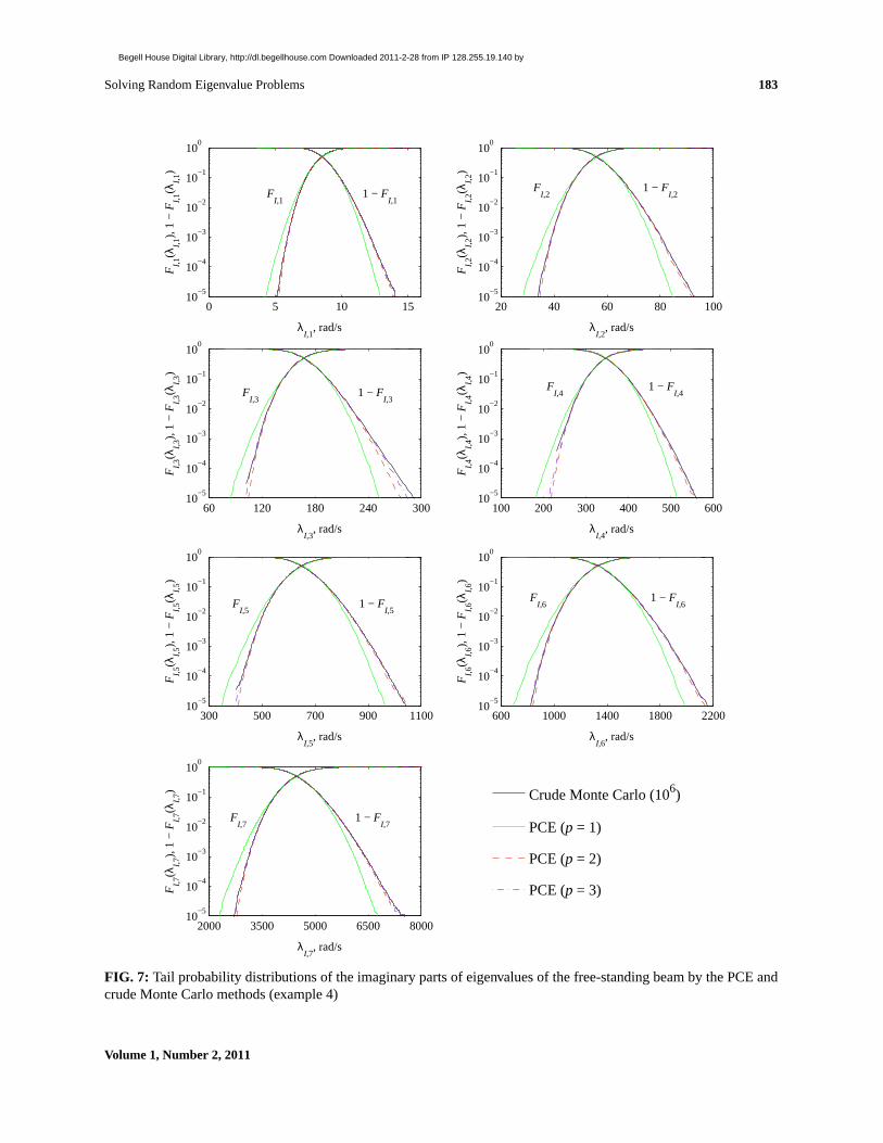
Due to nonproportional damping, the discrete beam model yields 14 complex eigenvaluesλi(X) = λR,i(X) ±√−1λI,i(X), i = 1, . . . , 7 in conjugate pairs, where the real partsλR,i(X) and imaginary partsλI,i(X) are bothstochastic. Using the PDD method, Fig. 6 presents the marginal probability distributionsFI,i(λI,i) and the com-plementary probabilities1 − FI,i(λI,i), i = 1, . . . , 7 of all seven imaginary parts, which also represent the naturalfrequencies of the beam. The distributionsFI,i(λI,i) and1 − FI,i(λI,i) at low probabilities describe tail character-istics of λi at the left and right ends, respectively. Each subfigure of Fig. 6 contains four plots: one obtained fromcrude Monte Carlo simulation and the remaining three generated from the univariate (S = 1), bivariate (S = 2), andtrivariate (S = 3) PDD approximations, employingm = 3, n = 4. In contrast, Fig. 7 displays the same probabilitydistributions of all seven imaginary parts of the eigenvalues calculated using the PCE method. Each subfigure of Fig. 7also contains four plots: one obtained from crude Monte Carlo simulation and the remaining three derived from thefirst-order (p = 1), second-order (p = 2), and third-order (p = 3) PCE approximations, employingn = p + 1.From Fig. 6 or 7, the tail probability distributions at both ends converge rapidly with respect toS or p, regard-less of the oscillatory mode. Therefore, both the PDD and PCE methods can be applied to solve this REP accura-tely.

To determine the computational efficiency of the PDD and PCE methods, Figs. 8a and 8b portray enlarged viewsof the tail probability distributions of the first and seventh natural frequencies, respectively, of the beam calculatedby all three variants of the PDD or PCE methods, including crude Monte Carlo simulation. Compared with crudeMonte Carlo simulation, the bivariate, third-order PDD approximation, trivariate, third-order PDD approximation,and third-order PCE approximation provide excellent estimates of the tail distributions. The results further indicatethat the bivariate, third-order PDD and third-order PCE approximations, both in consilience with the Monte Carlosolution, demand 613 and 5989 eigenvalue evaluations. Therefore, the PDD approximation is about5989/613 ∼= 10times more economical than the PCE approximation.

6.5 Example 5: Piezoelectric Transducer

The final example entails eigenspectrum analysis of a piezoelectric transducer commonly used for converting electri-cal pulses to mechanical vibrations, and vice versa. Figure 9a shows a 25 mm diam cylinder made of a piezoelectricceramic PZT4 (lead zirconate titanate) with brass end caps. The thicknesses of the transducer and end caps are 1.5and 3 mm, respectively. The cylinder, 25 mm long, was electroded on both the inner and outer surfaces. The randomvariables include: (i) ten nonzero constants defining elasticity, piezoelectric stress coefficients, and dielectric proper-ties of PZT4; (ii) elastic modulus and Poisson’s ratio of brass; and (iii) mass densities of brass and PZT4 [7]. Thestatistical properties of all 14 random variables are listed in Table 4. The random variables are independent and followlognormal distributions. Because of axisymmetry, a 20-noded finite-element model of a slice of the transducer, shownin Fig. 9b, was created. The model was considered to be open circuited. All natural frequencies calculated correspondto antiresonant frequencies.



182 Rahman & Yadav

2000 3500 5000 6500 800010

−5

10−4

10−3

10−2

10−1

100

λI,7

, rad/s

FI,

7(λI,

7), 1

− F

I,7(λ

I,7)

0 4 8 12 1610

−5

10−4

10−3

10−2

10−1

100

λI,1

, rad/s

FI,

1(λI,

1), 1

− F

I,1(λ

I,1)

20 40 60 80 10010

−5

10−4

10−3

10−2

10−1

100

λI,2

, rad/s

FI,

2(λI,

2), 1

− F

I,2(λ

I,2)

60 120 180 240 30010

−5

10−4

10−3

10−2

10−1

100

λI,3

, rad/s

FI,

3(λI,

3), 1

− F

I,3(λ

I,3)

100 200 300 400 500 60010

−5

10−4

10−3

10−2

10−1

100

λI,4

, rad/s

FI,

4(λI,

4), 1

− F

I,4(λ

I,4)

300 500 700 900 110010

−5

10−4

10−3

10−2

10−1

100

λI,5

, rad/s

FI,

5(λI,

5), 1

− F

I,5(λ

I,5)

Crude Monte Carlo (106)

Univariate PDD (m = 3)

Bivariate PDD (m = 3)

Trivariate PDD (m = 3)

600 1000 1400 1800 220010

−5

10−4

10−3

10−2

10−1

100

λI,6

, rad/s

FI,

6(λI,

6), 1

− F

I,6(λ

I,6)

FI,1

1 − FI,1

FI,2

1 − FI,2

1 − FI,4

FI,41 − F

I,3F

I,3

FI,5

1 − FI,5

FI,6

1 − FI,6

1 − FI,7

FI,7

FIG. 6: Tail probability distributions of the imaginary parts of eigenvalues of the free-standing beam by the PDD andcrude Monte Carlo methods (example 4)




0 5 10 1510

−5

10−4

10−3

10−2

10−1

100

λI,1

, rad/s

FI,

1(λI,

1), 1

− F

I,1(λ

I,1)

20 40 60 80 10010

−5

10−4

10−3

10−2

10−1

100

λI,2

, rad/s

FI,

2(λI,

2), 1

− F

I,2(λ

I,2)

60 120 180 240 30010

−5

10−4

10−3

10−2

10−1

100

λI,3

, rad/s

FI,

3(λI,

3), 1

− F

I,3(λ

I,3)

100 200 300 400 500 60010

−5

10−4

10−3

10−2

10−1

100

λI,4

, rad/s

FI,

4(λI,

4), 1

− F

I,4(λ

I,4)

300 500 700 900 110010

−5

10−4

10−3

10−2

10−1

100

λI,5

, rad/s

FI,

5(λI,

5), 1

− F

I,5(λ

I,5)


PCE (p = 1)

PCE (p = 2)

PCE (p = 3)

600 1000 1400 1800 220010

−5

10−4

10−3

10−2

10−1

100

λI,6

, rad/s

FI,

6(λI,

6), 1

− F

I,6(λ

I,6)

2000 3500 5000 6500 800010

−5

10−4

10−3

10−2

10−1

100

λI,7

, rad/s

FI,

7(λI,

7), 1

− F

I,7(λ

I,7)

FI,1

1 − FI,1

FI,2

1 − FI,2

1 − FI,4

FI,41 − F

I,3F

I,3

FI,5

1 − FI,5

FI,6

1 − FI,6

1 − FI,7

FI,7

FIG. 7: Tail probability distributions of the imaginary parts of eigenvalues of the free-standing beam by the PCE andcrude Monte Carlo methods (example 4)



184 Rahman & Yadav

2200 2400 2600 2800 300010

-5

10-4

λI,7

, rad/s

FI,

7(λ

I,7)

4 4.5 5 5.5 610

-5

10-4

λI,1

, rad/s

FI,

1(λ

I,1)


Univariate PDD (m = 3)

Bivariate PDD (m = 3)

Trivariate PDD (m = 3)

PCE (p = 1)

PCE (p = 2)

PCE (p = 3)

(a) (b)

FIG. 8: Comparisons of tail probability distributions of the imaginary parts of eigenvalues of the free-standing beamby the PDD, PCE, and crude Monte Carlo methods (example 4): (a)λI,1 and (b)λI,7

Brass cap

Brass cap

11 mm 11 mm1.5 mm

(a)

Electroded surfaces

Ceramic

(a)

3 mm

12.5 mm

3 mm

12.5 mm

11 mm 1.5 mm

Electroded surfaces

Brass cap

Ceramic

(b)

FIG. 9: Piezoelectric transducer: (a) geometry and (b) finite-element discrete model

Figure 10 presents the marginal probability distributions of the first six natural frequencies,Ωi, i = 1, . . . , 6, ofthe transducer by the bivariate (S = 2), third-order (m = 3) PDD and third-order (p = 3) PCE methods, respectively.These probabilistic characteristics, obtained by settingn = m+1 = p+1 = 4, are judged to be converged responses,as their changes due to further increases inm andp are negligibly small. Therefore, the PDD and PCE methodsrequire 1513 and 24,809 ABAQUS-aided FEA, respectively—a significant mismatch in computational efforts—in




TABLE 4: Statistical properties of the random input for the piezoelectriccylinder

Random variable Property(a) MeanCoefficient of

variationX1, GPa D1111 115.4 0.15X2, GPa D1122, D1133 74.28 0.15X3, GPa D2222, D3333 139 0.15X4, GPa D2233 77.84 0.15X5, GPa D1212, D2323, D1313 25.64 0.15X6, Coulomb/m2 e111 15.08 0.1X7, Coulomb/m2 e122, e133 –5.207 0.1X8, Coulomb/m2 e212, e313 12.71 0.1X9, nF/m D11 5.872 0.1X10, nF/m D22, D33 6.752 0.1X11, GPa Eb 104 0.15X12 νb 0.37 0.05X13, g/m3 ρb 8500 0.15X14, g/m3 ρc 7500 0.15

(a)Dijkl are elastic moduli of ceramic;eijk are piezoelectric stress coeffi-cients of ceramic;Dij are dielectric constants of ceramic;Eb, νb, ρb areelastic modulus, Poisson’s ratio, and mass density of brass;ρc is massdensity of ceramic.

generating all six probability distributions. Due to expensive FEA, crude Monte Carlo simulation was conductedonly up to 50,000 realizations, producing only rough estimates of the distributions. Given the low sample size, thedistributions from crude Monte Carlo simulation, also plotted in Fig. 10, are not expected to provide very accuratetail characteristics. Nonetheless, the overall shapes of all six probability distributions generated by both expansionmethods match these Monte Carlo results quite well. However, a comparison of their computational efforts once againfinds the PDD method wringing computational savings more than the PCE method by an order of magnitude in solvingthis practical eigenvalue problem.

7. CONCLUSIONS

Two stochastic expansion methods originating from PDD and PCE were investigated for solving REPs commonlyencountered in stochastic dynamic systems. Both methods comprise a broad range of orthonormal polynomial basesconsistent with the probability measure of the random input and an innovative dimension-reduction integration forcalculating the expansion coefficients. A new theorem, proven herein, demonstrates that the infinite series from PCEcan be reshuffled to derive the infinite series from PDD and vice versa. However, compared with PCE, which containsterms arranged with respect to the order of polynomials, PDD is structured with respect to the degree of cooperativitybetween a finite number of random variables. Therefore, significant differences exist regarding the accuracy, efficiency,and convergence properties of their truncated series.

An alternative form of the PCE approximation expressed in terms of the PDD expansion coefficients was devel-oped. As a result, the probabilistic eigensolutions from both the PDD and PCE methods can be obtained from thesame PDD coefficients, leading to closed-form expressions of the second-moment properties of eigenvalues and re-spective errors. For a class of REPs, where the cooperative effects of input variables on an eigenvalue get progressivelyweaker or vanish altogether, the error perpetrated by the PCE approximation is larger than that committed by the PDDapproximation, when the expansions orders are equal. Given the same expansion orders, the PDD approximation in-



186 Rahman & Yadav

0 10 20 3010

10

10

10

10

100

ω1, kHz

F1(ω

1)

0 20 40 60 8010

10

10

10

10

100

ω2, kHz

F2(ω

2)

0 20 40 60 8010

10

10

10

10

100

ω3, kHz

F3(ω

3)

20 40 60 80 10010

10

10

10

10

100

ω4, kHz

F4(ω

4)

40 60 80 100 12010

10

10

10

10

100

ω5, kHz

F5(ω

5)

60 80 100 120 14010

10

10

10

10

100

ω6, kHz

F6(ω

6)

Crude Monte Carlo (50,000) Bivariate PDD (m = 3) PCE (p = 3)

-5

-4

-3

-2

-1

-5

-4

-3

-2

-1

-5

-4

-3

-2

-1

-5

-4

-3

-2

-1

-5

-4

-3

-2

-1

-5

-4

-3

-2

-1

FIG. 10: Marginal probability distributions of the first six natural frequencies of the piezoelectric transducer by thePDD, PCE, and crude Monte Carlo methods (example 5)

cluding main and cooperative effects of all input variables cannot be worse than the PCE approximation, although theinclusion of all cooperative effects undermines the salient features of PDD.

The PDD and PCE methods were employed to calculate the second-moment properties and tail probability dis-tributions in five numerical problems, where the output functions are either mathematical functions involving smoothpolynomials or nonpolynomials or real- or complex-valued eigensolutions from dynamic systems, some requiringFEA. The second-moment errors from the mathematical functions indicate rapid convergence of the PDD and PCEsolutions, easily outperforming the sampling-based methods. Moreover, for the functions examined, the convergencerates of the PDD method are noticeably higher than those of the PCE approximation. The same trend was observedwhen calculating the variance of a two-degree-of-freedom linear oscillator regardless of the number of random vari-ables. A comparison of the numbers of eigenvalue evaluations (numbers of FEA), required for estimating with thesame accuracy the frequency distributions of a free-standing beam and a piezoelectric transducer, finds the PDD ap-proximation to be more economical than the PCE approximation by an order of magnitude or more. The computational




efficiency of the PDD method is attributed to its dimensional hierarchy, favorably exploiting the hidden dimensionalstructures of stochastic responses, including random eigensolutions, examined in this work.

ACKNOWLEDGMENTS

The authors acknowledge financial support from the U.S. National Science Foundation under Grant No. CMMI-0653279.

REFERENCES

1. Boyce, W. E.,Probabilistic Methods in Applied Mathematics I, Academic Press, New York, 1968.

2. Mehlhose, S., Vom Scheidt, J., and Wunderlich, R., Random eigenvalue problems for bending vibrations of beams,Zeit.Angew. Math. Mech., 79:693–702, 1999.

3. Grigoriu, M., A solution of the random eigenvalue problem by crossing theory,J. Sound Vib., 158(1):69–80, 1992.

4. Nair, P. B. and Keane, A. J., An approximate solution scheme for the algebraic random eigenvalue problem,J. Sound Vib.,260(1):45–65, 2003.

5. Adhikari, S. and Friswell, M. I., Random matrix eigenvalue problems in structural dynamics,Int. J. Numer. Methods Eng.,69:562–591, 2007.

6. Ghosh, D., Ghanem, R. G., and Red-Horse, J., Analysis of eigenvalues and modal interaction of stochastic systems,AIAA Jo.,43:2196–2201, 2005.

7. Rahman, S., Probability distributions of natural frequencies of uncertain dynamic systems,AIAA J., 47(6):1579–1589, 2009.

8. Gautschi, W.,Orthogonal Polynomials: Computation and Approximation, Oxford University Press, London, 2004.

9. Rahman, S., Extended polynomial dimensional decomposition for arbitrary probability distributions,J. Eng. Mech.,135(12):1439–1451, 2009.

10. Rahman, S., Statistical moments of polynomial dimensional decomposition,J. Eng. Mech., 136(7):923–927, 2010.

11. Wiener, N., The homogeneous chaos,Am. J. Math., 60(4):897–936, 1938.

12. Ghanem, R. G. and Spanos, P. D.,Stochastic Finite Elements: A Spectral Approach, Springer-Verlag, Berlin, 1991.

13. Xiu, D. and Karniadakis, G. E., The Wiener-Askey polynomial chaos for stochastic differential equations,SIAM J. Sci. Com-put., 24:619–644, 2002.

14. Rahman, S., A polynomial dimensional decomposition for stochastic computing,Int. J. Numer. Methods Eng., 76:2091–2116,2008.

15. Xu, H. and Rahman, S., A generalized dimension-reduction method for multi-dimensional integration in stochastic mechanics,Int. J. Numer. Methods Eng., 61:1992–2019, 2004.

16. IMSL Numerical Libraries,User’s Guide and Theoretical Manual, Visual Numerics, Houston, Texas, 2005.

17. ABAQUS Standard, Version 6.9, Dassualt Systems Simulia Corp., 2010.

18. Sudret, B., Global sensitivity analysis using polynomial chaos expansions,Reliab. Eng. Sys. Safety, 93(7):964–979, 2008.

19. Ishigami, T. and Homma, T., An importance quantification technique in uncertainty analysis for computer models,Proceedingsof the ISUMA ’90, 1st International Symposium on Uncertainty Modeling and Analysis, University of Maryland, pp. 398–403,1990.

20. Rahman, S., Stochastic dynamic systems with complex-valued eigensolutions,Int. J. Numer. Methods Eng., 71:963–986, 2007.



orthogonal polynomial expansions for - college of

Documents