Finance and Economics Discussion Series Divisions of Research & Statistics and Monetary Affairs

Federal Reserve Board, Washington, D.C.

Gestation Lags for Capital, Cash Flows, and Tobin’s Q

Jonathan N. Millar 2005-24

NOTE: Staff working papers in the Finance and Economics Discussion Series (FEDS) are preliminary materials circulated to stimulate discussion and critical comment. The analysis and conclusions set forth are those of the authors and do not indicate concurrence by other members of the research staff or the Board of Governors. References in publications to the Finance and Economics Discussion Series (other than acknowledgement) should be cleared with the author(s) to protect the tentative character of these papers.

Gestation Lags for Capital, Cash Flows, and Tobin's QJonathan N. Millar�Board of Governors of the Federal Reserve SystemThis version: May 10, 2005Abstra tInvestment models typi ally assume that apital be omes produ tive al-most immediately after pur hase and that there is no lead time neededto plan. In this ase, marginal q is usually suÆ ient for investment.This paper develops a model of aggregate investment where ompeti-tive �rms fa e no adjustment osts other than building and planningdelays. In this ontext, both Tobin's Q and ash ow an be noisy indi- ators of investment be ause some sho ks fail to outlast the ombinedgestation lag. The paper demonstrates some empiri al fa ts that hal-lenge prevailing theories of investment but are onsistent with gestationrequirements. Regressions using aggregate data suggest that it takes atleast four quarters for investment to respond to te hnology sho ks and asmany as eight additional quarters before produ tive apa ity is a�e ted.Estimates from stru tural VARs show that only permanent sho ks af-fe t investment, but that ash ow and Q rea t to both permanent andtransitory sho ks.�The author would like to thank Matthew Shapiro, Miles Kimball, Dmitriy Stolyarov,Tyler Shumway, Bill Was her, Darrel Cohen, and seminar parti ipants at the University ofMi higan and the Board of Governors of the Federal Reserve System for many substantive omments and suggestions. The views in this paper are solely the responsibility of theauthor and should not be interpreted as re e ting the views of the Board of Governors ofthe Federal Reserve System or its sta�.

I. Introdu tionInvestment models typi ally assume that (1) apital expenditures o ur im-mediately after the �rm's investment de ision, and (2) that pur hased apitalbe omes produ tive with little or no delay. These features ontrast with pra -ti al a ounts of investment, where proje ts often require onsiderable periodsof planning and building. The planning period en ompasses the time neededfor engineers to draw up the details, lawyers to obtain relevant permits, andmanagement to arrange �nan ing. Building involves the time needed for on-stru tion and for equipment to be ordered, delivered, and installed. Owing tothese delays, there may be a onsiderable lag between the de ision to in rease apa ity and the ommen ement of produ tion in a new fa ility.In the neo lassi al world, the user ost adjusts to equate the (fri tionless)demand for apital servi es with supply. In this environment, the urrentshadow value of a �rm's apital yields no useful information for investmentbe ause its realized value is always equal to one. Although there is some evi-den e that this fri tionless relationship holds in the very long run, e onomistshave long re ognized the short omings of this theory at higher frequen ies.1Adjustment ost models have emerged as the dominant paradigm to �ll thistheoreti al gap. In these models, deviations from the neo lassi al apital equi-librium are the result of an optimizing pro ess where �rms weigh the ostsand bene�ts of faster adjustment. When adjustment osts are onvex, thepro ess of apital adjustment is smooth and the urrent value of q ompletelyen apsulates all of the �rm's relevant investment onsiderations.2 The em-piri al short omings of this framework have prompted more re ent modelsthat de-emphasize q as an investment indi ator.3 These models emphasizethe lumpiness of investment at the plant and �rm levels in the presen e ofnon- onvex adjustment osts.However, the osts of apital adjustment are not always measured justin resour e osts and lost produ tion|they may also be re koned in time.These lags ause ompli ations for apital adjustment that are interesting and1Caballero [1994℄ shows a long run relationship between the neo lassi al user ost andthe apital sto k.2Although q is not generally observable, Hayashi [1982℄ demonstrates that, under ertain onditions, the urrent Tobin's Q is an exa t measure of q.3Some well- ited short oming of the onvex adjustment ost model are that (1) invest-ment is too lumpy at the plant and �rm-level to be explained by onvex adjustment osts(Doms and Dunne [1998℄), (2) that ash ows seem to apture some relevant informationfor investment by �nan ially- onstrained �rms that is not aptured in Q (Fazzari, Hubbard,and Peterson [1988℄), and (3) that Q is subje t to measurement error (Eri kson and Whited[2000℄). 1

important in their own right. Be ause invested apital be omes produ tivewith a delay, �rms must base urrent investment de isions on fore asts ofwhat variables like q and ash ow will be when the new apital omes on line.As a result, many of familiar ontemporaneous linkages between investment, q,and the value of the apital servi e ow do not hold after the fa t. Empiri altesting is ompli ated by the fa t that we observe realizations of variableslike Q and ash ow rather than the anti ipated values that are the basisof investment de isions. Further, time lags tend to spread out the responseof investment and produ tive apa ity to sho ks, leading to ri her dynami e�e ts.These building and planning lags have some history in the real business y le literature. The seminal work is Kydland and Pres ott [1982℄, who add atime to build lag for apital to a alibrated RBC model. A more re ent ontri-bution by Christiano and Todd [1995℄ adds a planning phase to the Kydlandand Pres ott setup. These models suggest that apital gestation requirements an apture some empiri al features of the business y le more e�e tively thanstandard models with one building period or models with onvex apital ad-justment osts.4 There are also some noteworthy attempts to onsider ges-tation lags in the investment literature. Majd and Pindy k [1987℄ explorethe impli ations of pla ing a eiling on the amount of investment that anbe undertaken ea h period in the pro ess of assembling a single (irreversible) apital proje t. Investment outlays only ontinue when the anti ipated dis- ounted value of the ompleted proje t ex eeds a minimum threshold. Altug[1993℄ takes a detailed look at apital pri ing and investment de isions in thepresen e of Kydland and Pres ott building requirements. She shows that ad-ditions to the apital sto k depend on the fore ast of marginal q after thebuilding period, whi h may not be well proxied by the urrent Tobin's Q.In the next se tion of this paper, I develop a model of aggregate investmentin a ompetitive e onomy in whi h �rms fa e distin t planning and buildinglags for new apital, but no other expli it adjustment osts. The e onomy issubje t to temporary and permanent aggregate sho ks that �rms an distin-guish at the moment they o ur. These features yield important impli ationsfor investment, the rate of ash ow, and Tobin's Q. Investment only respondsto sho ks that are expe ted to outlast the gestation horizon, and then onlyafter the planning phase is omplete. In ontrast, both the rate of ash owand Q respond to all sho ks throughout their duration, o-varying positively4Christiano and Todd emphasize that a ombined building and planning lag an a ountfor the persistent e�e ts of te hnologi al sho ks, the tenden y for business and stru turesinvestment to lag movements in output, and the leading relationship of produ tivity to hoursworked. 2

with asso iated investment during the building period. As a result, both ash ow and Q tend to be noisy indi ators of investment, where the orrelationdepends on the relative preponderan e of temporary and permanent sho ksin the data. The model also yields impli ations for the dynami response ofinvestment and produ tive apa ity to sho ks. The planning phase ausesa delay in the response of investment spending, while building auses a lagbetween investment spending and the asso iated in rease in produ tion.Se tion III performs some empiri al analysis. First, data for \puri�ed"Solow residuals are used to show that distin t planning and building lagsexist, and to estimate their duration. Then, I estimate empiri al impulseresponses of aggregate investment, ash ow, and Tobin's Q to temporaryand permanent sho ks, and ompare these responses to the predi tions of thegestation lag model and other well-known alternatives from the investmentliterature. These impulse responses are estimated using a stru tural VARthat identi�es temporary and permanent aggregate disturban es using the zerofrequen y restri tions of Shapiro and Watson [1988℄ and Blan hard and Quah[1989℄. Among other things, the gestation lag model orre tly predi ts thataggregate investment is driven almost entirely by permanent sho ks, while ash ow and Q respond to both sho ks. In addition, aggregate investment exhibitsa delayed response to permanent sho ks that is onsistent in hara ter to themodel's predi tions, and in onsistent with models that have no gestation lag.Se tion IV on ludes the paper with some dis ussion of the major results.II. ModelLet time to plan denote the P periods that begin with the de ision to addprodu tive apital, and end when investment expenditures ommen e. Timeto build denotes the B periods that begin with the �rst apital expenditure,and end when the new apital be omes produ tive. Following Kydland andPres ott [1982℄, assume that a proportion �j 2 [0; 1℄ of the planned apitaladdition is a quired j periods before it be omes produ tive apital, so thatPB�1j=0 �B�j = 1. These lags are depi ted graphi ally in Figure 1. At time t,a �rm ommits to hange its apital sto k at period t+P+B. The P periodplanning phase then passes where there are no investment outlays asso iatedwith the plan. At t+P , the building phase begins, with the �rm arrying outa non-negative proportion �B�j of the total expenditure asso iated with theplan at ea h period t+P+j, from j = 0; : : : ; B � 1, with �B > 0. The new apital be omes available for produ tion at t+P+B, after a total gestation lagof J=P+B periods. 3

Note that ea h investment plan is assumed to be irrevo able in the sensethat the �rm ommits to a spe i� level of apital at the end of its gestationperiod. This assumption is ne essary be ause the planning lag is meaninglesswhen investment plans an be hanged without ost. More spe i� ally, thesolution to any intertemporal optimization problem requires a plan for ea h ontrol variable for every period in the problem horizon. However, the ontrolvariables an be hanged ostlessly when the problem is revisited in subsequentperiods, so these plans are not binding. The irrevo ability assumption makesthis ost in�nite for ommitted plans. Nonetheless, there is no restri tion thatinvestment plans be non-negative, so the irrevo ability assumption is not thesame as irreversibility. Firms an plan to dismantle their apital in subsequentperiods, albeit with the same gestation requirement.In the remainder of this se tion, I develop a model for the investment, ash ows, and value of an aggregate �rm that fa es the gestation lags des ribedabove. The �rm operates in a ompetitive small open e onomy that is subje tto temporary and permanent sto hasti sho ks to te hnology and the supplyof labor. As su h, all market pri es are treated as given, and the interest rateexogenous. The ompetitive e onomy assumption is omparable to Hayashi[1982℄, whi h many ite as a justi� ation for using Tobin's Q as a proxy forthe shadow value of new apital. Yet unlike Hayashi, the unit of analysis isan aggregate �rm. This is di tated by the fa t that the optimal apital sto kof an individual ompetitive �rm is indeterminate when produ tion exhibits onstant returns to s ale, so its optimal rate of investment is not well de�ned.5This indetermina y is not an important issue for the aggregate �rm, be auseequilibrium in the markets for other variable inputs pins down the aggregate apital sto k.6 The fo us on a small open e onomy de-emphasizes a host ofdynami general equilibrium onsiderations that may not be relevant whenthe e onomy is open for trade in apital and goods. Moreover, this approa hallows for a more transparent depi tion of some issues related to gestationlags that have been largely negle ted by previous work, su h as the role oftemporary apital s ar ity in the investment-Q relationship.The model development pro eeds as follows. I begin by spe ifying theprodu tion te hnology for the aggregate �rm and �nd optimal losed-form so-lutions for the apital growth rate, the rate of ash ow, and Tobin's Q ina de entralized equilibrium. Rather than expli itly solving the de entralized5Although the s ale of an individual �rm in Hayashi's model is also indeterminate, itsrate of investment is pinned down by a �rst order ondition that links q to the marginaladjustment ost for apital.6In his textbook, Romer [1996℄ adopts a similar approa h for his dis ussion of investmentwith adjustment osts, albeit in redu ed form.4

problem to �nd these solutions, I employ a number of strategies to simplifythe exposition. Sin e the de entralized solution will be eÆ ient, I obtain thesame optimality onditions for the produ tion side by maximizing the value ofan aggregate �rm that treats pri es as given, then imposing that the marginalprodu t of ea h input equal its market rental rate. I do not bother to set outoptimal household onsumption onditions be ause these an be ignored inthe small open e onomy a ording to the Fisher separation theorem. Finally,I in orporate household labor de isions in a stylized manner by introdu inga redu ed-form aggregate labor supply urve. The resulting model is used todes ribe in detail the interrelationships between ash ow, investment, and Q.I lose the se tion by dis ussing measurement issues that arise from the exis-ten e of apital building requirements, and how they a�e t the interpretationof model results. 1. Cash FlowFor now, ignore the intertemporal aspe ts of the problem. Let urrentoutput be the numeraire. Assume that the aggregate �rm enters the urrentperiod with a predetermined produ tive apital sto k K and level of te hnol-ogy ZT , and hooses the quantity of labor L that maximizes variable pro�ts.Although the impli ations of the more general CES produ tion fun tion willalso be onsidered, for expositional purposes it is useful (and onsiderablymore tra table) to assume the Cobb-Douglas produ tion fun tion(1) F �K;ZTL� = K1�� �ZTL�� :Units of labor an be hired at the given market wage rate w. After maximizingout the variable fa tor L, the aggregate �rm's variable pro�t is(2) �� �Kjw;ZT ; �� = (1� �) �h�ZTw � �1�� K;where � is the orporate tax rate, and �h � (1� �)� �1�� . Let the rate of ash ow denote the average variable pro�t of apital:(3) �� �w;ZT ; �� = (1� �) �h�ZTw � �1�� :Sin e total ash ows are linear inK, this fun tion is also the marginal produ tof apital. This equation an also be interpreted as a fa tor pri e possibilityfrontier that shows the negative relationship between the labor wage and thevalue of apital servi es with te hnology is held �xed. Sin e the Cobb-Douglas ase embeds a unit elasti ity of substitution between apital and labor the5

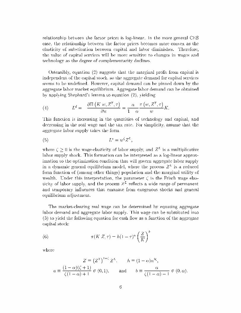
relationship between the fa tor pri es is log-linear. In the more general CES ase, the relationship between the fa tor pri es be omes more onvex as theelasti ity of substitution between apital and labor diminishes. Therefore,the value of apital servi es will be more sensitive to hanges in wages andte hnology as the degree of omplementarity de lines.Ostensibly, equation (2) suggests that the marginal pro�t from apital isindependent of the apital sto k, so the aggregate demand for apital servi esseems to be unde�ned. However, apital demand an be pinned down by theaggregate labor market equilibrium. Aggregate labor demand an be obtainedby applying Shephard's lemma to equation (2), yielding(4) Ld = ��� �Kjw;ZT ; ���w = �1� � �� �w;ZT ; ��w K:This fun tion is in reasing in the quantities of te hnology and apital, andde reasing in the real wage and the tax rate. For simpli ity, assume that theaggregate labor supply takes the form(5) Ls = w�ZL;where � � 0 is the wage-elasti ity of labor supply, and ZL is a multipli ativelabor supply sho k. This formation an be interpreted as a log-linear approx-imation to the optimization ondition that will govern aggregate labor supplyin a dynami general equilibrium model, where the pro ess ZL is a redu edform fun tion of (among other things) population and the marginal utility ofwealth. Under this interpretation, the parameter � is the Fris h wage elas-ti ity of labor supply, and the pro ess ZL re e ts a wide range of permanentand temporary in uen es that emanate from exogenous sho ks and generalequilibrium adjustment.The market- learing real wage an be determined by equating aggregatelabor demand and aggregate labor supply. This wage an be substituted into(3) to yield the following equation for ash ow as a fun tion of the aggregate apital sto k: �(KjZ; �) = h(1� �)a�ZK�b(6)where Z � �ZT �1+� ZL; h � (1� �)�b�;a � (1� �)(� + 1)�(1� �) + 1 2 (0; 1); and b � ��(1� �) + 1 2 (0; �):6

This fun tion represents the marginal ontribution of apital servi es to vari-able pro�ts in any given period, or the aggregate inverse demand urve for apital servi es. In a fri tionless world, this is set equal to the neo lassi aluser ost to determine the urrent apital sto k. The fa tor Z, whi h ombinesboth sho ks to te hnology and labor supply, neatly en apsulates the exogenous(non-tax) fa tors that shift the aggregate demand for apital servi es.The parameter b represents the elasti ity of ash ow with respe t to the apital imbalan e ratio K=Z, after a ounting for endogenous movements inlabor. In the Cobb-Douglas ase, b is bounded in magnitude between zeroand by labor's share �. For the more general CES produ tion fun tion, b isinversely related to the elasti ity of substitution between labor and apital.Although a solution of the form in (6) is not generally available when theprodu tion fun tion is CES, a log-linear approximation an be al ulated forthe spe ial ase where the labor supply elasti ity � is zero. Then the elasti ityof ash ow with respe t to apital imbalan e in the steady state is sh�L=�,where � is the onstant substitution elasti ity between apital and labor, andsh�L is labor's share of in ome in the steady state. Intuitively, this indi atesthat redu ed substitutability between apital and variable inputs makes thevalue of apital more sensitive to its degree of aggregate s ar ity.2. Investment with Gestation Lags of Arbitrary DurationNow onsider the intertemporal aspe ts of the optimization problem re-lating to investment. This optimization determines a plan for the aggregate apital sto k from the gestation horizon onward, subje t to the onstraintsimposed by the predetermined quantities of apital for periods within the ges-tation horizon. Viewed from the perspe tive of the so ial planner, this pathequates the ex ante value of apital servi es (the anti ipated rate of ash ow)to its ex ante so ial ost. This is shorthand for the apital market equilibriumthat would be determined, passively, by the intera tion of atomisti de isionsin the de entralized e onomy. From the perspe tive of the aggregate �rm, theoptimal plan maximizes its market value, taking as given the anti ipated pathof future pri es and the rate of ash ow. The aggregate �rm negle ts thein uen e of its own apital sto k on the rate of ash ow be ause its prob-lem represents the a umulated de isions of individual �rms that, in isolation,have a negligible in uen e on the value of apital. Consequently, the aggregate�rm a ts like a small �rm that fa es onstant returns to s ale in produ tion,per eiving no well-de�ned solution for its optimal apital path. Instead, theoptimal path of apital is pinned down by the apital market equilibrium.Let sk;t represent, at time t, the planned addition to the produ tive apital7

sto k in k periods. Then, the produ tive apital sto k evolves a ording tothe a umulation ondition(7) Kt+i = Kt+i�1(1� Æ) + s1;t+i�1;where Æ is the depre iation rate. This di�ers from the standard a umulationidentity be ause the addition to the produ tive sto k is di tated by the planfrom J periods earlier rather than urrent investment. Committed plans evolvesu h that this period's planned addition at horizon k equals the next period'splan for horizon k�1, so that(8) sk�1;t+i+1 = sk;t+i;for k=2;: : : ;J . The total investment ow in ea h period is the sum of spendingon all ommitted plans that are in the building pro ess:(9) It+i = BXj=1 �jsj;t+i:Consequently, the investment ow is not generally asso iated with any spe i� plan; rather, it a moving average of planned additions over the next B periods.Given this stru ture, there are many state variables that must be onsideredin the optimization problem. At time t, the �rm inherits its urrent produ tive apital sto k, along with planned additions for the next J�1 periods, yieldinga total of J state variables. Note that these plans are relevant to the problem,although they are not yet part of the produ tive apital sto k, be ause theywill a�e t the optimal apital addition at the gestation horizon.Now onsider the problem from the perspe tive of the aggregate �rm. Forsimpli ity, the appropriate dis ount fa tor is onstant at R = 1+ r, where r isthe interest rate. New units of apital an be pur hased for a �xed pri e of �p,whi h is net of the value of any government tax in entives.7 Sin e anti ipatedrates of ash ow are onsidered given, the appropriate notion of variable pro�tis ��K, where �� represents the fun tion (3). The market valuation of �rm is thedis ounted total of all future expe ted ash ows, net of investment outlaysunder the optimal plan:(10) V (Kt; fsj;tgJ�1j=1 j�p; ft��t+ig1i=0) � maxfsJ;t+ig1i=0 1Xi=0 R�i [t��t+iKt+i � �pIt+i℄ ;7This in ludes both an investment tax redit � and the present value of apital onsump-tion allowan es z. These in entives e�e tively redu e the pri e of new apital by a fa tor(1� �� z), where �+ z is the tax wedge. 8

subje t to the onstraints (7) through (9). The �rm solves this problem byplanning additions to its apital sto k from period t+J onward. However, onlythe plan for t+J binds future de isions.8 Note that ��t+i is a fun tion of the given(but not exogenous) market real wage wt+i, so the valuation problem re e tsexpe ted onditions in the labor market (and, by impli ation, the anti ipatedpath of Z) ontingent on urrent information.It is useful to restate this problem as a series of unrelated intratemporalproblems. Tedious manipulation that (among other things) utilizes equations(7) through (9) to eliminate the ow variables It+i and sJ;t+i for i>0 yields:(11) V (Kt; fsj;tgJ�1j=1 j�p; ft��t+ig1i=0)� �pq�0Kt + �p B�1Xi=1 q�i si;t + J�1Xi=0 R�i � t�t+i�p � u�� �pKt+i+R�J maxfKt+J+ig1i=0 1Xi=0 R�i � t�t+J+i�p � u�� �pKt+J+i;where u� is de�ned as the steady state user ost of apital, and q�i is the steadystate shadow value of apital that is i= 0;: : : ;B�1 periods from joining theprodu tive apital sto k, re koned in terms of new apital. These values are onsidered given be ause they are fun tions of the interest rate and parameters.This depi tion of the problem an be interpreted as follows. The �rst two terms olle tively represent the value of all funds ommitted to produ tive apitaland ongoing onstru tion. The shadow values, whi h are al ulated as(12) q�i � BXj=i+1Rj�i�j for i = 0; : : : ; B � 1;represent the future value of all the outlays that were ne essary to a quirethe apital at its urrent stage of ompletion. For instan e, to obtain a unitof ompleted produ tive apital today (i = 0), the �rm must pur hase �junits of new apital at time t�j, whi h is worth �jRj in today's terms after ompensating for foregone interest. These payments are summed for j=1 toB to obtain the total shadow value q�0. It an easily be seen that q�0 ex eedsone. Intuitively, this ompensates for the interest foregone on apital outlaysduring the unprodu tive building period. Also, note that the apital outlays8Equation (10) an be amended to in orporate the personal taxes and depre iation al-lowan es the �rm holds for its existing apital. Let tg and td represent the tax rates on apital gains and dividends, respe tively, and let ~Zt represent the present value of the re-maining apital onsumption allowan es on the �rm's existing apital. Then, the value ofthe �rm be omes ~V = R(1�td)R�tg (V + ~Zt), where R = 1 + r1�tg in (10).9

asso iated with a given plan do not a�e t the value of the �rm until the outlayhas taken pla e.The third set of terms in (11) aptures the value of the quasi-rents thatthe �rm expe ts to earn on its produ tive apital during the gestation period.These anti ipated rents o ur be ause the �rm annot adjust its produ tive apital to re e t new information until the end of the gestation horizon. Therent in ea h period is the di�eren e between the ash ow (re koned in termsof apital) and the steady state user ost of apital u�, multiplied by thea quisition value of the apital. The steady state user ost is given by(13) u� � q�0 � (1� Æ)R�1q�0;whi h represents the total opportunity ost of obtaining a unit of apital ser-vi es for the urrent period only. This is the steady state value of a unit ofprodu tive apital q�0 today less pro eeds that ould be obtained from sellingthe undepre iated portion of the installed apital next period.The �nal set of terms in (11) represents the value of the quasi-rents thatthe �rm expe ts to earn from the urrent gestation horizon onward. At thispoint, it is useful to temporarily onsider the problem from the so ial planner'sperspe tive. From this viewpoint, it is optimal for these anti ipated rents tobe zero so that the marginal so ial ost of apital is equal to its marginalso ial bene�t. This requires the steady state user ost of apital to equal theanti ipated ash ow from the gestation horizon onward, so that(14) t��t+J+i�p = u� for all i � 0:This implies that ash ow is always expe ted to return to its long run ben h-mark of u� at the end of the gestation horizon. The �rm's optimal plans mustbe onsistent with this anti ipated market equilibrium, so this ondition e�e -tively pins down the path of ash ows (and, in turn, produ tive apital) fromthe gestation horizon onward. Consequently, the �nal set of terms in (11) arealways zero, so they drop out of the problem.Condition (14) an be used to determine the equilibrium aggregate ap-ital sto k for period t+J and non-binding plans for the aggregate sto k insubsequent periods. Using equations (6) and (14), one an determine that:(15) Kt+J = �h(1� �)a�pu� � 1b Et[Zbt+J ℄ 1b :Note that the quantity of apital is based upon a fore ast of Z, rather thanits realization. Therefore, the apital sto k an only respond to unanti ipated10

movements in the fa tor Z with a lag. Moreover, transitory movements inZ that are not expe ted to outlast the gestation horizon will never a�e t the apital sto k. Despite this, the apital sto k does move roughly in proportionwith the demand for apital servi es in the long run.9These statements an be established formally by assuming that the apitaldemand fa tor Zt follows an exogenous pro ess. For simpli ity, I approximatea �nite-order ARIMA using the IMA form(16) lnZt+1 = lnZt + �+ �(L) t+1 +�(L)�t+1;where �t+s and t+s, are normally distributed iid sho ks with zero mean andunit varian e. The parameter � is (approximately) the expe ted rate of growthin the level of fri tionless apital demand. �(L) and �(L) are the followingpolynomials in the lag operator L:�(L) � nTXi=0 �iLi; and �(L) � nGXi=0 iLi;(17)where nT is a positive integer, and nG is a non-negative integer. It is assumedthat there is a unit root in the MA polynomial �, whi h ensures that only the t sho ks have a permanent e�e t upon the sequen e fZt+sg1s=0.10Now onsider the rate of growth in the apital sto k, given the exogenouspro ess for Z des ribed above. Although it need not be generally true, assumefor expositional purposes that �(L) = 0 = , so that the permanent portionof Z is a random walk. Let gKt = � lnKt denote the growth rate in the apitalsto k at t, where � is the �rst-di�eren e operator 1�L. By equation (15), thisgrowth rate is(18) gKt+J = 1b �lnEt[Zbt+J ℄� lnEt�1[Zbt+J�1℄� :Substituting the onditional expe tations of Zbt+j for j =J and j=J�1 intothis equation yieldsgKt+J = �+ t + �t min(J;nT )Xi=0 �i + min(nT�J;0)Xi=1 �J+i�t�i:The growth rate in produ tive apital at t+J is equal to the un onditionalgrowth rate �, plus adjustments for the anti ipated e�e t of sho ks dated t9Note that by Jensen's inequality, Et[Zbt+J ℄ 1b < Et[Zt+J ℄, so E[Kt℄ 6� E[Zt℄.10Further, assume that the umulative sum of the MA oeÆ ients in �(L) and �(L) arenever negative up to any lag. This ensures that the umulative e�e t of ea h sho k is alwaysin one dire tion. 11

and earlier on the rate of growth in the apital demand fa tor Z. The dynami e�e ts of these sho ks are summarized by the impulse responses�gKt+j��t = 8><>:0 j < JPmin(J;n)i=0 �i j = J�j j > J and �gKt+j� t = 8><>:0 j < J j = J0 j > J :Sho ks never a�e t produ tive apital growth until the end of the gestationhorizon J , be ause they were not observable when the apital plans were om-mitted. At the gestation horizon (j=J), apital growth generally has a large at h-up response to the anti ipated umulative e�e t of the sho k on the de-mand for apital servi es. For a permanent sho k, the response of produ tive apital growth is on�ned to horizon J . No further adjustment is required atsubsequent horizons, be ause the extra demand for apital is fully re e tedin the apital sto k. In omparison, a temporary sho k may not a�e t thegrowth rate of apital at all if it is suÆ iently short-lived (so that nT < J).More generally, a temporary sho k will prompt produ tive apital growth athorizon J if it outlasts the gestation horizon. However, this will eventuallybe a ompanied by negative apital growth in subsequent periods, sin e thetemporary sho k has no e�e t on the fri tionless demand for apital servi esin the long run.11 As the length of the gestation horizon in reases, it be omesin reasingly unlikely that temporary sho ks will outlast the gestation horizonand prompt investment. Provided that the gestation horizon is suÆ ientlylong, apital growth will only be asso iated with permanent sho ks.3. The Relationship of Investment to Cash Flow and Tobin's QIn this se tion I onsider the relationship between the growth rate in pro-du tive apital and two variables that are ommonly used as indi ators forinvestment, the rate of ash ow and Tobin's Q.By equation (14), the rate of ash ow is always expe ted to return to thesteady state user ost at the end of the urrent gestation horizon. Despitethis, the realized demand for apital servi es at this long run user ost willnot generally be equal to the �xed ow of apital servi es available to the �rmin any given period. This is be ause the quantity of produ tive apital wasdetermined J periods earlier, using in omplete information. As a result, the11This fa t an be demonstrated as follows:limj!1 � lnKt+j��t = limj!1 jXi=1 �gKt+i��t = limj!1min(j;nT )Xi=0 �i = �(1) = 0:12

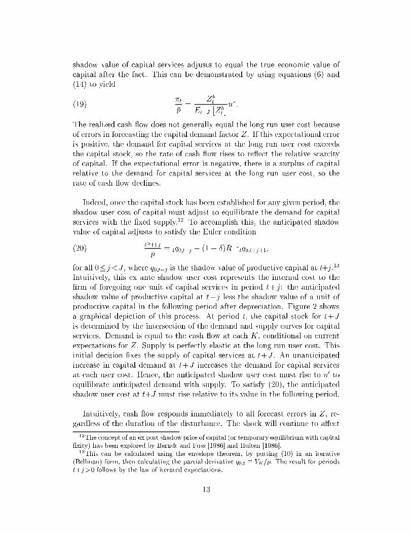
shadow value of apital servi es adjusts to equal the true e onomi value of apital after the fa t. This an be demonstrated by using equations (6) and(14) to yield(19) �t�p = ZbtEt�J �Zbt �u�:The realized ash ow does not generally equal the long run user ost be auseof errors in fore asting the apital demand fa tor Z. If this expe tational erroris positive, the demand for apital servi es at the long run user ost ex eedsthe apital sto k, so the rate of ash ow rises to re e t the relative s ar ityof apital. If the expe tational error is negative, there is a surplus of apitalrelative to the demand for apital servi es at the long run user ost, so therate of ash ow de lines.Indeed, on e the apital sto k has been established for any given period, theshadow user ost of apital must adjust to equilibrate the demand for apitalservi es with the �xed supply.12 To a omplish this, the anti ipated shadowvalue of apital adjusts to satisfy the Euler ondition(20) t�t+j�p = tq0;t+j � (1� Æ)R�1tq0;t+j+1;for all 0�j<J , where q0;t+j is the shadow value of produ tive apital at t+j.13Intuitively, this ex ante shadow user ost represents the internal ost to the�rm of foregoing one unit of apital servi es in period t+j: the anti ipatedshadow value of produ tive apital at t+j less the shadow value of a unit ofprodu tive apital in the following period after depre iation. Figure 2 showsa graphi al depi tion of this pro ess. At period t, the apital sto k for t+Jis determined by the interse tion of the demand and supply urves for apitalservi es. Demand is equal to the ash ow at ea h K, onditional on urrentexpe tations for Z. Supply is perfe tly elasti at the long run user ost. Thisinitial de ision �xes the supply of apital servi es at t+J . An unanti ipatedin rease in apital demand at t+J in reases the demand for apital servi esat ea h user ost. Hen e, the anti ipated shadow user ost must rise to u0 toequilibrate anti ipated demand with supply. To satisfy (20), the anti ipatedshadow user ost at t+J must rise relative to its value in the following period.Intuitively, ash ow responds immediately to all fore ast errors in Z, re-gardless of the duration of the disturban e. The sho k will ontinue to a�e t12The on ept of an ex post shadow pri e of apital (or temporary equilibrium with apital�xity) has been explored by Berndt and Fuss [1986℄ and Hulten [1986℄.13This an be al ulated using the envelope theorem, by putting (10) in an iterative(Bellman) form, then al ulating the partial derivative q0;t � VK=�p. The result for periodst+j>0 follows by the law of iterated expe tations.13

the rate of ash ow until the apital sto k has had a han e to fully adjust tothe additional apital demand. This an be established formally by using theexogenous pro ess for Z in (16) and equation (19) to al ulate the followingimpulse responses for temporary and permanent sho ks:� ln�t+j��t = (bPmin(j;n)i=0 �i 0 � j < J0 otherwise ; and � ln�t+j� t = (b 0 � j < J0 otherwise :Generally, the e�e t of any sho k on ash ow depends on the magnitude ofthe sho k and the elasti ity fa tor b. At impa t, a sho k raises ash ow by theprodu t of b and the impa t MA oeÆ ient. To the extent that it persists, asho k an a�e t future ash ows up to the gestation horizon. For a horizon ofj periods after the sho k, the e�e t depends on the umulative sum of theMA oeÆ ients up to lag j. Intuitively, this sum represents the umulative e�e tof the sho k on the fore ast error for Zb. Neither temporary nor permanentsho ks a�e t ash ow at the gestation horizon or beyond, on e apital has theability to adjust. The ex post rents aused by sho ks are always unanti ipatedand transitory, as one would expe t in a ompetitive market.The degree of o-movement between the rate of ash ow and investmentdepends on the nature of the sho k. For permanent sho ks, the o-movementis positive. Cash ow responds to the sho k immediately, and ontinues to bea�e ted to the end of the gestation horizon. Although growth in the produ -tive apital sto k is postponed to the gestation horizon and beyond, invest-ment spending ommen es at the planning horizon P . Therefore, both ash ow and investment respond in the same dire tion during the building period.Temporary sho ks with a duration shorter than the gestation horizon do notprompt investment, so there is no positive o-movement. Temporary sho ksthat outlast the gestation horizon may ause investment to o-move positivelyor negatively with ash ow. In order for a temporary sho k to a�e t apitalgrowth, it must also a�e t ash ow up to the end of the gestation horizon, inthe same dire tion as the sho k. If this is the ase, the investment response atthe building horizon is in the same dire tion as ash ow. However, sin e thetemporary sho k annot a�e t the level of the apital sto k in the long run,the positive initial response of investment must eventually be reversed withnegative investment. Some of this negative investment may o ur while ash ow remains elevated within the building phase. Nonetheless, it is reasonableto expe t the orrelation between investment and ash ow to be positive,on balan e, with the strength of the orrelation depending on the relativepreponderan e of temporary and permanent sho ks in the e onomy.Tobin's Q is usually al ulated as the urrent market value of a �rm dividedby the repla ement value of its urrent apital sto k. For now, assume that14

the repla ement value of apital is measured as the repla ement value of theprodu tive apital sto k. Then (11) an be used to determine that(21) Qt = q�0 + B�1Xi=1 si;tKt q�i + J�1Xi=0 R�i � t�t+i�p � u�� Kt+iKt :The �rst two terms in (21) represent the value of the funds ommitted toprodu tive apital and ongoing building e�orts, per unit of produ tive apital.The un onditional value of these two terms generally ex eeds one, for tworeasons. As demonstrated earlier, the un onditional shadow values in orporate ompensation for foregone interest during the gestation period. As well, theplanned apital additions si;t are generally positive owing to e onomi growth.Therefore, when there are gestation lags, this measure of Q should ex eed onein the long run. The �nal term shows that Q re e ts the anti ipated value ofe onomi rents looking forward over the entire gestation horizon.Sin e Q re e ts both the value of produ tive apital and of ommittedplans, it is not equivalent to the shadow value of produ tive apital q0;t. InAppendix A, I demonstrate that(22) Qt = q0;t + J�1Xi=1 qi;t si;tKt ;where qi;t is the urrent shadow value of si;t. Further, I show that the shadowvalue of produ tive apital is its steady state value, plus the dis ounted valueof all anti ipated rents during the gestation period:(23) q0;t = q�0 + J�1Xj=0 � R1� Æ��j � t�t+j�p � u�� ;where the dis ount fa tor in ludes (1 � Æ) in order to ompensate for theopportunity ost of depre iation. This on�rms that both q and Q re e t thesame e onomi rents that a�e t ash ow. As �ltrations of the same sho kpro ess they provide similar e onomi information.Moreover, neitherQt nor q0;t onsistently provide reliable information about urrent investment. Re all that the apital sto k is determined by equatingthe anti ipated demand for apital servi es to the long run user ost of apitalu�. This orresponds to setting tq0;t+J equal to the �xed long run shadow valueq�0. Consequently, the deviation between the realization of q0;t+J and q�0 is afore ast error that must be orthogonal to produ tive apital growth at t+J .However, urrent values of Qt and q0;t o-move with investment to the extent15

that sho ks to Z reate unanti ipated rents during the building phase of thegestation period. In addition, there will be a response in Q owing to the dire te�e t of investment expenditures on the value of the �rm during the buildingpro ess. Intuitively, a permanent sho k to Z a�e ts Qt (and q0;t) on impa t, by ausing anti ipated rents during the entire gestation horizon. Both variablesrespond in the dire tion of the sho k throughout the gestation period be auserents persist over time. At the planning horizon, investment expendituresbegin to respond to the sho k. Therefore, both Qt and q0;t ovary positivelywith investment during the building pro ess. However, as with ash ow, this o-movement breaks down for temporary sho ks that are not suÆ iently long-lived to prompt investment. When this is the ase, movements in Qt (and q0;t)are unrelated to investment.These laims an be on�rmed formally using impulse responses for thelog-linearized value of Qt. Using the log-linearization in Appendix B, theimpulse responses an be al ulated using the responses for ash ow and apital growth, yielding� lnQt+j� t � B�1Xi=1 �i�gKt+j+i� t + J�1�jXi=0 !i� ln�t+j+i� t= 8>>>>><>>>>>:b J�1�jPi=0 !i 0 � j � P �J�j + b J�1�jPi=0 !i P < j < J � 10 j � J ; and� lnQt+j��t � B�1Xi=1 �i�gKt+j+i��t + J�1�jXi=0 !i� ln�t+j+i��t= 8>>>>><>>>>>:

J�1�jPi=0 !ibmin(j;n)Pi=0 �i 0 � j � P�J�j min(J;n)Pi=0 �i+max(j�P�1;0)Pk=1 �J�j+k�J+k+J�1�jPi=0 !ibmin(j;n)Pi=0 �i P < j < J � 1B�1Pk=1 �k�j+k j � J :Here, �i is the (semi-)elasti ity of Qt with respe t to apital growth at hori-zon i. In the appendix, I demonstrate that this elasti ity is de reasing in i.The parameter !i is the elasti ity of Q with respe t to ash ow at horizoni, whi h also de reases in i for reasonable alibrations. These responses re- e t three lear phases. The �rst phase oin ides with the planning horizon,with Q in reasing to re e t the present value of anti ipated rents throughoutthe remainder of the gestation period. The value of these anti ipated rents16

eventually de line as a new long equilibrium be omes imminent, be ause thehorizon over whi h they o ur be omes smaller. However, this e�e t neednot be strongest on impa t. If the sho k has suÆ ient duration to promptinvestment, there is a se ond phase in whi h Q rises to re e t the value ofnon-produ tive apital as it is a umulated throughout the building phase.This e�e t be omes stronger as the new long run equilibrium approa hes. Fi-nally, a third phase may arise for temporary sho ks that outlast the gestationhorizon. In this phase, the apital sto k ontinues to adjust downward as thesho k dies out over time. In this phase, there are no rents, but Q de lines tore e t the value of ongoing disinvestment.4. A Re on iliation Between Measured Capital and Produ tive CapitalThe results above require produ tive apital to be measured using an a - ounting s heme that orre tly a ounts for building lags. In pra ti e, mea-sures of the apital sto k are usually formed under the assumption of onebuilding period.14 Therefore, the estimate of the apital sto k at any point intime in ludes both ompleted and in omplete apital. Consequently, standardstatisti al measures of Qt, apital growth, and ash ow do not oin ide withthe true produ tive measures des ribed above.One strategy for dealing with this problem is to use investment expendituresto onstru t measures of the apital sto k that a ount for alternative buildinglags. However, this is unsatisfa tory be ause it imposes a lag stru ture on thedata. The strategy adopted in this paper is to �nd a mapping from a ountingmeasure to the unobserved measure of produ tive apital. This mapping anthen be in orporated into the interpretation of statisti al results, allowing thedata to tell its story.Let ~Kt denote the a ounting measure of the apital sto k at t, formedusing a standard one period time to build apital a umulation identity. InAppendix C, I show that the produ tive measure of apital, K, maps to thisa ounting measure by the lag polynomial(24) ~Kt+1+i = �(L)Kt+B+i; where �(L) = BXj=0 �B�jLj:This is simply a generalization of the standard a ounting relationship, whi h orre tly measures the produ tive apital sto k in the spe ial ase where J=14With the ex eption of ele tri light and power stru tures, the BEA does not makean expli it attempt to adjust for building lags for most types of apital. The pra ti e isjusti�ed by the fa t that the aggregate value of un ompleted plants has been a small andstable proportion of the value of ompleted plants through time (see BEA [1999℄).17

B = 1 and �1 = 1.15 In this general ase, the a ounting measure ~Kt+1 is aweighted average of the planned sto ks of produ tive apital from t+1 to t+B,with the weight at horizon j equal to the spending proportion �B�j. Providedthat there is a building period, the a ounting measure in orporates hangesin the produ tive apital sto k before they o ur.It is also useful to determine a mapping from the a ounting measure of apital growth to the true produ tive measure. De�ne ~gKt+i as the rate ofgrowth in a ounting apital, � ln ~Kt+i. The appendix shows that this mapsto the true produ tive measure by the lag polynomial(25) ~gKt+1+i � ~�(L)gKt+B+i; where ~�(L) = BXj=0 ~�B�jLj;and ~�(1) = 1. Again, this generalizes the standard ondition, whi h orre tlymeasures produ tive apital in the spe ial ase where J =B=1. The growthrate in the statisti al measure is approximately a weighted average of thegrowth rates in the produ tive apital sto k over the next B periods. Theweights ~�j are losely related to the true spending weights �j.16The responses des ribed earlier in this se tion an be translated to aseswhere apital is measured using the standard a ounting. A ounting apitalgrowth never re e ts sho ks until the planning horizon is omplete. Thereafter,a planned addition to produ tive apital works its way through the buildingphase, a�e ting the observed measure of apital growth by the amount that it hanges spending in ea h period. This an be seen using the equations�~gKt+j� t � 8><>:0 j � P~�J�j+1 �gKt+J� t J > j > P0 j > J ; and�~gKt+j��t � 8><>:0 j � Pmin(j�P;B�1)Pi=0 ~�B�i �gKt+B+j�i�1��t j > P :These responses show that the measured apital growth asso iated with anyplan is spread throughout the building period. For example, onsider a per-manent sho k t that in reases gKt+J by one per entage point. Due to the15Note that this also embeds a spe ial ase where there is no time to build, so �0 = 1. Forthis ase, the end-of-the-period statisti al measure, after urrent investment, is the a tualquantity of produ tive apital during the period.16The weights ~�j give slightly more importan e to spending at longer horizons j than �j ,and less importan e to shorter horizons. 18

planning lag, the sho k doesn't a�e t observed apital growth up to t+P+1.During the building phase, the sho k a�e ts observed apital growth by ~�jper entage points in ea h period, where j is the number of periods to the endof the gestation horizon. On e the building period is omplete, there are nofurther e�e ts on observed apital growth.Sin e ~Kt is used to al ulate measures of ash ow and Q, dis repan iesbetween produ tive apital and the a ounting measure also a�e t how thesevariables respond to sho ks. The a ounting measures of ash ow and Q arerelated to their true produ tive measures by(26) ln ~�t+i = ln�t+i � ln ~Kt+iKt+i and ln ~Qt+i = lnQt+i � ln ~Kt+iKt+i :Applying a linear approximation yields that(27) d ln ~Kt+iKt+i � ~�(L)dgKt+B+i; where ~�(L) = B�1Xj=0 ~�B�jLj;and ~�B�j = ~�B + : : : + ~�j. Therefore, the hange in the \error" asso iatedwith mismeasurement of the apital sto k is related to a distributed lag of thegrowth rates in produ tive apital over the building horizon.This measurement dis repan y a�e ts the interpretation of the impulse re-sponses for ash ow and Q as follows. Up to the end of the planning horizonP , the error has no e�e t. Intuitively, this is be ause the a ounting measureof the apital sto k has not yet rea ted to the sho k. If the sho k has suÆ ientduration to prompt investment, the a ounting measure of the apital sto krises over the ourse of the building period. Therefore, it has a progressivelynegative in uen e on the impulse response. If b is below one, this e�e t eventu-ally be omes strong enough to outweigh the positive in uen e of rents on ash ow and Q, so the response be omes negative at suÆ iently long horizons.III. Empiri al Eviden e1. DataI onstru ted my dataset using quarterly aggregates for non-farm non-�nan ial U.S orporations from 1959Q2 to 2002Q4. Series for Tobin's Q, ash ows, and the growth rate in apital were onstru ted using seasonally-adjusted data from the Flow of Funds A ounts of the Federal Reserve Board,19

the Bureau of E onomi Analysis (BEA), the Bureau of Labor Statisti s (BLS),and Data Resour es International (DRI). The a ounting measure of the ap-ital sto k was generated iteratively using quarterly �xed investment expendi-tures and a one period time-to-build apital a umulation identity.17 FollowingHall [2001℄, I al ulate the measure of the aggregate market value of physi al apital as the value of equity and debt, less the value of all non- apital assets(in luding liquid assets), residential stru tures, and inventories. Both Tobin'sQ and ash ows are adjusted to a ount for orporate in ome taxes and thein uen e of investment tax redits and depre iation allowan es on the e�e -tive pri e of apital. A detailed des ription of the data onstru tion is givenin Appendix F.Time plots of the data are shown in Figures 3 to 5. Table 1 ontains samplemoments. Figure 3 demonstrates the onsiderable volatility in apital growth,whi h exhibits many prolonged movements around a mean of about 1.1 per entper quarter. Cash ows and Tobin's Q are plotted in Figures 4 and 5, respe -tively. Sin e the tax orre tion for the pri e of apital goods de reases therepla ement value of the a ounting measure of apital, it auses a noti eablein rease in both series. The measure of Q is very volatile, and does not seemto revert to a dis ernable long run level. Rather, the series is hara terized byits many high-frequen y movements around prolonged, low-frequen y trends.Note from Table 1 that the sample average of the tax- orre ted measure iswell above one, whi h is onsistent with the gestation model for apital. Cash ow seems to y le around a stable long run mean, with movements resem-bling the business y le. Although there are periods where ash ow and Qexhibit oheren e with investment, neither is a onsistent indi ator. Despitethis, the three variables have positive mutual orrelation, whi h is apparentby inspe tion of the plots.Visually, it appears that the Q series may be non-stationary. Table 2 ex-plores this possibility using the Augmented Di key Fuller test and the Varian eRatio test. The Di key Fuller test reje ts a unit root in ~gKt and ~�t, but fails toreje t for ~Qt. This is problemati for most investment theories, sin e Q shouldrevert to a well-de�ned long run level. Inspe tion of Figure 5 suggests thatthis failure may re e t very low-frequen y movements in the level of Q, whi h ould be explained by a number of fa tors, in luding, for example, hangesin the e�e tive tax rate on apital gains and dividends, or hanges in ompo-nents of �rm value that are outside of the model, su h as intangible apital17A pre-sample for the apital sto k was generated for the period 1947Q1 to 1959Q1 inorder to minimize the possibility of errors asso iated with an appropriate starting value.The initial value for the end of 1946 was set equal to the BEA's estimate of the real apitalsto k. 20

(Hall [2001℄).18 Varian e ratios for Q diminish onsiderably at longer horizons,whi h provides eviden e against a unit root.2. The Existen e and Duration of Gestation LagsIn this se tion, I use tests involving Solow residuals and labor hours growthto onsider two distin t issues. The �rst issue is whether there is a delayedresponse of investment to aggregate sho ks, whi h I interpret as a planninglag. The se ond issue is whether there is a delayed response of produ tive apital to investment, whi h would be asso iated with a building lag.John Fernald kindly provided quarterly Solow residuals for the period 1965Q2to 2001Q4 that are orre ted for measurement errors owing to hanges in laborquality and variable fa tor utilization using the methodology in Basu, Fernald,and Shapiro [2000℄.19 The Solow residuals are divided by a labor share of� = 2=3 to onvert to units of labor-augmenting te hnologi al progress. Quar-terly data for aggregate labor hours of non-�nan ial orporations are from theBLS. Figure 7 shows a time plot of the puri�ed Solow residuals and the growthrate in aggregate labor hours.i. Eviden e from Previous WorkThere have been a few attempts to measure the duration of the gestationperiod using ase studies at the plant and �rm level, and other non-parametri methods. Estimates by Koeva [2000℄, Mayer [1960℄ and Krainer [1968℄ sug-gest that the apital gestation lag ranges between one and two years. Mayer[1960℄ and Jorgenson and Stephenson [1967℄ obtain estimates of the planningduration ranging between six months and a year.20ii. PlanningMost prominent models do not feature a delayed response of apital growthto sho ks. To illustrate this, onsider the e�e t of a positive permanent sho k.18The valuation data are not adjusted to re e t hanges in the tax rate on dividends andthe apital gains rate, so there may be some trends owing to this mismeasurement. Summers[1981℄ and M Grattan and Pres ott [2002℄ demonstrate that hanges in these tax rates anhave large e�e ts on �rm value.19This study makes an additional adjustments for apital adjustment osts and for thereallo ation of resour es a ross se tors, whi h I remove for the purpose of my al ulations.20This eviden e is supported by stru tural VAR estimates by Er eg and Levin [2003℄using aggregate data, who �nd a seven quarter lag in the response of business investmentto monetary sho ks. 21

In the fri tionless neo lassi al model, investment should respond to the sho kimmediately, with the maximum rate of response at impa t. In a model with onvex adjustment osts, the investment response is also largest on impa t,but is more drawn out over time. Models with �xed adjustment osts, su h asCaballero and Engel [1999℄, and irreversibility, su h as Abel and Eberly [1993℄,tie the likelihood of investment to the degree of departure from the fri tionlessdemand for apital servi es. Provided that the sho k is not too large, generallysome �rms will invest, and some will not. This implies that aggregate apitalgrowth depends on the distribution of the apital imbalan es for all �rms in thee onomy. Sin e some �rms are prompted to invest in response to an aggregatesho k, neither of these issues ompli ate the initial timing of the aggregateresponse, only the magnitude. To get the maximum bene�t, most �rms thatdo adjust should do so immediately.21To investigate whether there is a planning lag in response to te hnologysho ks, I estimated the following equation using OLS:(28) ~gKt+1 = 0 + nsrXi=0 di ~srt�i + e1t;where ~srt�i is the puri�ed Solow residual at lag i. To onserve degrees of free-dom, I hose a maximum lag length of 14 quarters, whi h seems a reasonablebound for the total gestation horizon given the previous resear h dis ussedabove. This spe i� ation nests all possible planning and building ombina-tions as spe ial ases. Given the generalized form of the growth rate in thea ounting measure of apital in (25),(29) d~gKt+1d ~srt�P�i = BXj=0 ~�B�j dgKt+B�jd ~srt�P�i = dP+i; for i = 0; : : : ; B:Most investment models make the impli it assumption that P = 0 and thateither ~�0 = 1 or ~�1 = 1. Sin e these models suggest an immediate responseof produ tive apital growth at the building horizon, d0 should be positive. Ifthere is a planning lag, dP should be the �rst positive oeÆ ient, and P shouldbe an estimate of the planning horizon.The magnitude of the estimated oeÆ ients an be given a stru tural inter-pretation in the gestation lag model for a spe ial ase where te hnology andlabor supply disturban es are un orrelated, and the te hnology pro ess is a21Although it is possible that some �rms might rea h their investment trigger faster inthe following periods (due to depre iation), it seems doubtful that this e�e t would omposemost of the response. 22

random walk. For this ase, the results of Appendix D show thatdP+i = ~�B�i (1 + �) :Empiri al estimates of the wage-elasti ity of aggregate labor supply � rangebetween 0 and 1. For the spe ial ase where � = 0, the oeÆ ient dP+i shouldbe a dire t estimate of the spending share ~�B�i.Results for this regression are shown in Table 3. CoeÆ ient estimates areinsigni� ant up to the fourth lag, whi h is signi� ant at ten per ent. Thissuggests a planning period for investment of one year, whi h is at the highend of previous estimates by Mayer [1960℄ and Jorgenson and Stephenson[1967℄. Thereafter, the oeÆ ients for lags �ve through ten are ea h signi� antat levels of �ve per ent or lower. This suggests a planning lag of four or�ve quarters. The magnitude of the oeÆ ients at lags four through sevenindi ate that about 13 per ent of the investment expenditures asso iated witha given plan o ur during this time window. If the tenth lag is interpretedas the end of the building horizon, the estimates suggest a total gestationperiod of ten quarters, with a building phase from period four to period ten.However, this interpretation is subje t some important aveats. In prin iple,the building period should be measured by the delay between the initial hangein investment spending and the time it begins to a�e t produ tive apital.Sin e it is possible for building to ontinue with little or no expenditures, thismay not a urately re e t the length of the building horizon. A se ond on ernwith this interpretation is that the signi� an e of the lagged oeÆ ients beyondthe initial planning stage may re e t a planning period ombined with onvexadjustment osts for apital and/or prolonged general equilibrium adjustment.In the absen e of labor supply endogeneity, the oeÆ ients di, i = P; : : : ; Jshould sum to one over the building period. The tests reported in the bottomportion of Table 3 show that the umulative sum of the oeÆ ients up to thetenth lag is about one fourth, falling well short of the required ben hmark interms of magnitude and signi� an e. Among other things, this failure mayre e t in onsisten y in the regression estimates owing to measurement erroror endogeneity. Another plausible explanation is the presen e of external ad-justment osts in general equilibrium. In dynami general equilibrium modelsthat exhibit the balan ed growth property, it is well known that permanentte hnology sho ks prompt an equivalent umulative response in apital growth.However, due to the smoothing of onsumption and labor, the response willtend to be drawn out over time even in the absen e of internal adjustment ostsand/or apital gestation lags. Reasonably alibrated RBC models suggest thatit takes the e onomy between three to six quarters to omplete one-fourth ofthe total apital growth mandated by a permanent te hnology sho k. In the23

ben hmark ase of Campbell [1994℄, whi h features Cobb-Douglas produ tion,�xed labor, and unit intertemporal substitution elasti ity, the e onomy takesabout seven quarters to omplete one-fourth of the mandated apital growth.22Indeed, this smoothing e�e t be omes more pronoun ed as the durationof the gestation period in reases. Figure 9 shows the response of measured apital growth to a permanent te hnology sho k in a alibrated RBC model, forbuilding lags ranging from one to nine quarters. In ea h ase, it is assumed thatexpenditures are distributed evenly throughout the building period. Detailsof the model setup and alibration are outlined in Appendix E. A ordingto these simulations, the time required to omplete one fourth of the totaladjustment in reases exponentially with the building horizon, rising from sevenquarters with TTB=1, thirteen quarters with TTB=5, to 104 quarters withTTB=9. Given these results, the magnitude of the estimated oeÆ ients arenot unreasonable, nor is the notion that they ould be a reasonable out omefor an e onomy without expli it internal adjustment osts for apital.The regression results provide eviden e for a substantial planning lag. Notonly is there a delayed response of investment to sho ks, but the umulativeresponse up to the third lag is not signi� antly di�erent from zero. As well,the hara ter of the response is in onsistent with other models. The responseis a tually hump-shaped, peaking at the seventh lag. Most models withoutplanning would tend to have the largest response on impa t, or, most favorably,a at response out to some horizon. The estimated response is in onsistentwith these possibilities. To wit, the estimated umulative response from thefourth lag to the third lag is statisti ally larger than the estimated umulativeresponse from impa t to the third lag. Although these fa ts are hallenging toother models, they an easily be re on iled with planning and building lags.iii. BuildingBuilding involves the transformation of apital goods to produ tive apital.The time required for this transformation is not easily estimated, be auseprodu tive apital is not dire tly measurable. The strategy employed in thisse tion is based on the prin iple that hanges in produ tive apital ontributedire tly to output growth. Therefore, some portion of observed output growthmust be attributable to growth in the produ tive apital sto k.Applying the standard te hniques of growth a ounting to the simpli�edCobb-Douglas produ tion fun tion (1), one an obtain the following impli it22Adding a labor supply de ision tends to extend the period of adjustment, but notdramati ally. 24

measure of the growth rate in produ tive apital and te hnology:(30) ~mt � ~gYt � �~gHt = (1� �)gKt + srt;where ~gYt and ~gHt are the measured growth rates in output and labor, and srtis true te hnologi al growth. This suggests a stru tural equation of the form:(31) ~mt = �sr + (1� �)gKt + sr;twhere sr;t is a mean-zero random disturban e. In prin iple, this equationis a valid regression spe i� ation provided that the true te hnology sho k isorthogonal to the growth rate in produ tive apital, whi h is satis�ed if thereis at least a one-period time to build for apital. This suggests that one mightun over the length of the building period by regressing values of ~mt on lags of~gKt�j, where the signi� ant lagged oeÆ ient at the longest lag is an estimateof the building horizon.23Unfortunately, the above spe i� ation has undesirable properties that makethe results diÆ ult to interpret. Generally, there is no one-to-one mapping be-tween produ tive apital growth and measured apital growth. By inspe tionof (25), su h a mapping only exists for a spe ial ase where �B = 1, so thatgKt+B = ~gKt+1.24 For this spe ial ase, su h a regression would orre tly esti-mate the building horizon. This spe ial ase holds for any investment modelwith a standard one period building horizon (B = 1). For other ases, the hara teristi s of the mapping depend on the unobserved roots fxjgB�1j=1 of thelag polynomial ~�(x). Generally, there an be stable solutions for gKt forwardand ba kward (or both) in the observed measure ~gKt , where the roots anbe negative, positive, or omplex. This leads to ounterintuitive results that ompli ate the interpretation of the estimates.This an be illustrated using some simple examples. Consider a ase whereB=2, with ~�2=2/3 and ~�1=1/3. In this ase, the polynomial ~�(L) is simply(1+ :5L), whi h has a stable root of -2. For this very simple ase, the mappingis gKt = 32 1Xj=0 ��12�j ~gKt�1�j:Here, oeÆ ients on the lags of measured apital growth are non-zero fromthe �rst lag onward and have signs that os illate from negative to positive23The fa t that we are looking for the longest lag an easily be seen in Figure 1. Expen-ditures join the apital sto k sooner as the �rm nears the end of the building period.24Note that I assume that �B > 0 in order for the building horizon to be distinguishablefrom planning. This rules out other one-to-one mappings.25

at su essive lags. Although the oeÆ ients attenuate in magnitude at largerlags, it is highly plausible that estimates would yield signi� ant oeÆ ientsfor j � B. Therefore, the highest lag with a signi� ant oeÆ ient annotbe interpreted as an estimate of the building horizon. As a further example, onsider a ase where B=2 but ~�2 =1/3 and ~�1=2/3. In this ase, the rootof the lag polynomial ~�(L) is unstable at -0.5, and the mapping isgKt = �32 1Xj=0 ��12�j ~gKt+j:The suggested regression would have a signi� ant impa t oeÆ ient, but nosigni� ant oeÆ ients at any other lag. The results would in orre tly point toa one period building horizon.A less problemati stru tural spe i� ation an be obtained by ombiningequations (25) and (31) to obtain the following spe i� ation:~gKt+1 = b0 + BXj=1 bj ~mt+j + et; where(32) b0 � � �sr1� �; et � � BXj=1 ~�j1� � ~ sr;t+j; and bj � ~�j1� �for j = 1;: : : ;B. Here, observed apital growth depends on forward valuesof the impli it measure of apital growth and the te hnology disturban e. By onstru tion, the impli it measure ~mt is negatively orrelated to the error termbe ause it ontains the te hnology sho k sr. However, potential endogeneityproblems an be avoided by instrumenting for the forward values of ~mt+j.Finding an appropriate set of instruments is a thorny issue. First, the re-gression requires a lot of instruments. To avoid in onsisten y, the numberof in luded leads of ~mt should be no smaller than the building lag. To sat-isfy the order ondition, at least one instrument must be in luded for ea hlead. Se ond, although the set of valid instruments ontains the entire timet information set, most hoi es are likely to have limited strength be ausethe variation in ea h regressor is partially attributable to an unfore astablete hnology sho k. Nonetheless, some su ess was a hieved using urrent andlagged values of the measured growth rates in apital and labor hours. These hoi es were motivated by theoreti al onsiderations. In order to identify allthe spending shares ~�j, information about the growth rates in the produ tive apital sto k from t+1 to t+B must be in luded. Provided that te hnologysho ks are exogenous, serially un orrelated, and unfore astable, anything inthe time t information set is un orrelated to et. A ording to equation (25),26

measured apital growth at t re e ts the growth rate in produ tive apitalfrom t to t+B�1, while lags up to t+B�1 ontain additional identifyinginformation. However, these measures provide no information on gKt+B, leav-ing ~�T+B unidenti�ed. Under the model, planned additions to the produ tive apital sto k re e t information on labor growth from J periods earlier. Pro-vided that P > 0, labor growth from periods t to t�J+1 should ontain theneeded information, plus overidentifying information about the growth ratesfrom t+1 to t+B�1.Unfortunately, the estimates using this spe i� ation are likely to su�er froma signi� ant small sample bias. This is be ause the redu ed-form disturban eset are auto orrelated at lags up to B�1, whi h violates the Gauss-Markovassumptions. Therefore, tests that rely on asymptoti distributions will givemisleading results. To orre t for this problem, I generate bias- orre ted on-�den e intervals for the estimated parameters, using a bootstrap te hnique.25The results of the regression are shown in Table 4. The set of explanatoryvariables ontains twelve forward values of the ~mt+j, whi h are instrumentedusing measured rates of growth in apital and labor hours for lags rangingfrom zero to thirteen quarters. After orre ting for small-sample bias usinga bootstrap, the estimated oeÆ ients are statisti ally signi� ant at leads +2and from +4 through +8 at signi� an e levels of ten per ent or higher.26 Theestimates at the remaining leads are not di�erent from zero at signi� an elevels of at least ten per ent. This ould indi ate a la k of power against thenull, whi h is a reasonable assertion when the result is onsidered in onjun -tion with the other estimates. Nonetheless, the presen e of zero oeÆ ients atthese leads is not in onsistent with the theory. The partial R2 (Shea [1997℄)for ea h of the regressors is about 0.10, whi h raises the possibility of thesize distortions owing to weak instruments that are dis ussed by Bound et al.[1989℄, Sto k, Wright, and Yogo [2002℄, and others. These distortions may ause the true signi� an e level of the tests to be understated. Notwithstand-ing these possible distortions, the fa t that the partial R2 does not de linewith the forward lead o�ers partial support for the gestation lag story, as doesthe apparent e�e tiveness of deep lags as instruments. Considered olle tively,the estimates are suggestive of an eight-quarter building horizon, whi h is inline with the estimates that Koeva [2000℄ obtained using a non-parametri methodology. This estimate, ombined with the planning estimate of one yearobtained in the previous se tion, suggests a total gestation lag for new apital25In order to preserve the auto orrelation stru ture of the estimates in the bootstrapsimulation, I re-sample blo ks of twelve adja ent observations.26I report bias- orre ted intervals at a 90% signi� an e level. Intervals were also al ulatedfor signi� an e levels of 95% and 99%, for whi h I only report signi� an e.27

of about three years.A ording to the stru tural spe i� ation in (32), the oeÆ ients bj shouldsum to (1� �)�1 over the building horizon. Sin e apital's share of output isroughly 1/3 in aggregate data, the estimates should sum to about three. Amodel with a standard one-period time to build apital a umulation identityshould satisfy the restri tion that b1 = 3. The fa t that this null is easilyreje ted provides eviden e against this alternative. However, the null that the umulative sum of the estimated oeÆ ients is three annot be reje ted usingthe bootstrapped on�den e intervals, for signi� an e levels of ten per ent orhigher. If the building horizon is interpreted as eight periods, the 90% uppersigni� an e level is about 3.03, while at eleven periods, the upper limit rises toabout 3.78.27 This reinfor es the building horizon estimate of eight quarters.The reasonableness of an eight quarter building horizon an also be assessedusing an alternative test. A ording to the generalized pro ess for measured apital growth in (25), the un onditional auto orrelation of measured apitalgrowth at a given lag annot be zero unless that lag ex eeds the buildinghorizon.28 Beyond the building horizon, this orrelation should eventually goto zero, although it may extend beyond the building horizon if the growthrate in produ tive apital is serially orrelated. Therefore, an upper boundon the building horizon is the lag at whi h the un onditional auto orrelationof measured apital growth is statisti ally zero. Consider the orrelogram for~gKt in Figure 8. These orrelations suggest that the measured growth ratein apital is un onditionally auto orrelated up to ninth lag, at ten per entsigni� an e. This suggests an upper bound for the building period of ninequarters, slightly higher than the estimate obtained above.3. Temporary and Permanent InnovationsThis se tion estimates impulse responses to temporary and permanent ag-gregate sho ks that are identi�ed using the zero-frequen y restri tions em-ployed in other ontexts by Shapiro and Watson [1988℄ and Blan hard andQuah [1989℄. A ording to this s heme, only permanent sho ks an a�e t the apital sto k in the long run. This is a very weak restri tion that should besatis�ed in any model that onverges to a neo lassi al apital market equilib-rium in the long run. This in ludes standard investment models with onvex27Note that there may be a potential bias owing to endogeneity between the approximationerror in (25) and the instrumented regressors. Simulations by the author using a alibratedsystem (whi h an be obtained upon request) suggest that this auses a very small negativebias in large samples.28This holds be ause ov �~gKt ; ~gKt�j� > 0 for j=1: : :; B, provided that �j > 0.28

and non- onvex adjustment osts, transa tion osts, and irreversibility. Sin ethe identifying restri tion is reasonable for most models, the properties of theestimated impulse responses an be ompared to their respe tive predi tions.It is important to assess the models using reasonable standards, due to thenature of small-sample VAR estimation. It is typi al for identi�ed VARs toestimate a smooth impulse response, even if the data-generating pro ess hasmore well-de�ned hara teristi s. Moreover, most of the well-known resultsfrom alternative models are demonstrated in a partial equilibrium setting.Pri e adjustment in general equilibrium should tend to smooth results om-pared to these predi tions.29 Therefore, it is important to judge the modelsby their onsisten y with the general hara ter of the estimated responses.Some reasonable impli ations of the gestation lag model are as follows.Due to the planning lag, measured apital growth should respond sluggishlyto sho ks. If there is a signi� ant gestation horizon, measured apital growthshould rea t mu h more strongly to permanent innovations than to temporaryinnovations of the same magnitude. Given the sizable gestation lags estimatedabove, it would be reasonable to expe t little or no response of apital growthto temporary sho ks. Consequently, almost all of the varian e of investmentshould be attributable to permanent sho ks. In omparison, Q and the rate of ash ow should respond immediately to both disturban es, with the responselimited to the duration of the gestation horizon. The ompli ations that arisedue to the mismeasurement of produ tive apital should also be onsidered.For sho ks that prompt investment, ash ow should de line monotoni allyover the ourse of the building period, be ause the measured apital sto k (inits denominator) anti ipates the a tual produ tive sto k. This e�e t shouldnot o ur for Q, sin e it is roughly o�set by the e�e t of the �rm's ongoinga umulation of apital during the building period on market value. Signi� antproportions of the variation in Q and ash ow should be attributable to bothtemporary and permanent sho ks.Alternative models broadly imply that aggregate investment should respondimmediately to permanent sho ks. In a model with onvex adjustment osts,the response attenuates over time. Other models, su h as �xed adjustment osts and irreversibility, imply a more on entrated response. Broadly, thesemodels are well prote ted by a null that the response to the permanent sho k isnot upward-sloping over some horizon. The response to temporary sho ks foralternative models are more diÆ ult to assess. A non-positive response is evi-29For example, Thomas [2002℄ demonstrates that the lumpiness of mi ro-level investmentsuggested by a partial equilibrium model with transa tion osts will be smoothed onsider-ably in aggregate general equilibrium. 29

den e against a onvex adjustment ost model{if the sho k a�e ts q, it shouldprompt investment. In models with �xed adjustment osts or irreversibility,it is sensible to think that �rms are relu tant to adjust to temporary sho ks.However, there is little reason to believe that su h �rms would redu e invest-ment. With this in mind, a null that the response is non-negative is more thanadequate to prote t these models.I estimate two separate bivariate stru tural VARs. Spe i� ation (1) om-bines measured apital growth (in annual per entage terms) and the log ofmeasured ash ow (Y 1t = [~gKt+1; ln ~�t℄0), while spe i� ation (2) ombines the apital growth measure and the log of Tobin's Q (Y 2t = [~gKt+1; ln ~Qt℄0). For ea hsystem, I estimate a VAR of the formY jt = Bj0 +Bj1Y jt�1 + : : :+BjpY jt�p + ejt ; where E hejtej0t i = �j;and p is the number of lags.30 The estimated VARs for j = 1; 2 are then onverted to stru tural moving average form(33) Y jt = �jY + 1Xi=0 �ji � jt�i; �jt�i�0 ; where �jY = E [Yt℄ ;where jt�i and �jt�i are the permanent and temporary sho ks at time t � i,and the �ji are (2x2) matri es of stru tural oeÆ ients. The identi� ation ofea h system rests upon the assumption thatlims!1 � lnKt+s��t = lims!1 sXj=0 �gKt+1+j��t = 0;so that the hanges in the measured apital growth prompted by the temporarysho k sum to zero.Generally, the identi� ation methodology requires both variables in Yt tobe stationary, and the results are sensitive to departures from this ondition.This sensitivity is a ommon empiri al problem asso iated with zero-frequen y onstraints. For instan e, Blan hard and Quah [1989℄ make adjustments fornon-stationarity in the unemployment rate, from whi h they remove a �ttedlinear time trend. Re all that the eviden e for stationarity of Q is ambigu-ous: Di key-Fuller tests fail to reje t a unit root, while the varian e ratio testsuggests stationarity. To avoid problems asso iated with the potential non-stationarity of Q, I eliminated a very low frequen y trend using an HP �lter.3130The lag length is hosen a ording to the AIC.31The �lter was estimated with � = 99999. The results seem fairly robust to other hoi es.30

The rationale behind applying this �lter is that the s ope of the theory islimited to movements in Q up to the gestation lag. Arguably, the lower fre-quen ies re e t mismeasurement of tax e�e ts, intangibles, and other thingsthat are outside of the theory. Figure 6 shows the �tted trendline againsta tual Tobin's Q, in logs. The detrended series of (logged) Q is the a tualseries minus the trendline.For robustness, I report 90 per ent on�den e intervals estimated usingtwo alternative methods. The �rst intervals, whi h are denoted with \� ��," are al ulated using the asymptoti (normal) distribution of the impulseresponse (see L�utkepohl [1993℄). The se ond set of intervals, denoted with\��", employ the bootstrap-after-bootstrap method of Kilian [1998℄, whi his more robust in small samples.32Figures 10 and 11 show the impulse response estimates for spe i� ationsj=1; 2. In many respe ts, the hara ter of these responses is onsistent withthe predi tions of the gestation lag model. In both spe i� ations, apitalgrowth has a hump-shaped response to the permanent sho ks that, althoughsigni� ant on impa t, peaks at a lag of three to four quarters. The timing ofthis peak is roughly onsistent with the planning lag estimated in the previousse tion. Both responses remain positive and signi� ant at lags of up to 15quarters. Investment exhibits no signi� ant response to the temporary sho kin either spe i� ation. This is onsistent with the gestation lag model, butmay also be onsistent with irreversibility or transa tion ost models. Cash ow and Q respond to both temporary and permanent innovations in a similarmanner, peaking near the time of impa t, then attenuating to zero over time.The response of ash ow to the permanent sho k de lines faster than the orresponding response for Q, whi h is roughly onsistent with the model'spredi tion. Despite this, there is no eviden e that the ash ow responseeventually de lines below zero over the ourse of the building horizon.It is notable that the magnitude of the responses of ash ow and Q tothe temporary and permanent sho ks seem implausibly large relative to themeasured apital response given the predi tions of the gestation lag model.A ording to the derivations in Se tion II, the response of measured ash owto a permanent sho k should be no larger than b within the gestation period.In annual per entage terms, the response of measured apital growth at horizonP � j < J should be 400 ~�J�j. Sin e the expenditure shares sum to one, thissuggests that the ratio of the responses should average 400=bJ over the ourse32In all ases, I perform 5000 repli ations of the �rst stage of the bootstrap of the pro edure(whi h orre ts for bias in the estimated VAR oeÆ ients), and 5000 repli ations of these ond stage of the pro edure (whi h uses the orre ted oeÆ ient estimates).31

of the building horizon.33 When the produ tion fun tion is Cobb-Douglas, b an be no larger than labor's in ome share. Assuming that this share is about2=3, the ratio of the apital growth and ash ow responses should ex eed400~�B�j=b � 600~�B�j at any given horizon, and should be larger than 600=J ,on average. Cursory examination of Figure 10 suggests that the ratio falls wellbelow this magnitude for any reasonable gestation horizon. For instan e, theratio of the two responses averages around 25 for a gestation horizon of tenquarters, well below the minimal ben hmark of 60.One possible explanation for this dis repan y is that the degree of fa torsubstitutability imposed by Cobb-Douglas is too strong, whi h dampens themagnitude of the ex post rents predi ted by the theory. A greater degreeof omplementarity would magnify the sensitivity of ash ow (and Q) toimbalan es between the fri tionless demand for apital servi es and the �xed expost supply of produ tive apital. Re all that when the produ tion fun tion isCES and labor supply is inelasti , the magnitude of b is inversely proportionalto the elasti ity of substitution between apital and labor. For this ase, asubstitution elasti ity of 2=5 would be roughly suÆ ient to justify the relativemagnitudes of the apital and ash ow responses in the pre eding example forJ = 10. A low elasti ity of substitution would also explain why measured ash ow and Q fail to de line below zero over the ourse of the building horizon,be ause this only o urs when b < 1.The upper left-hand panels of Figures 12 and 13 test, for ea h spe i� a-tion, whether the upward-sloping hara ter of the investment response to thepermanent sho ks is statisti ally signi� ant. For ea h spe i� ation, these �g-ures show the �rst-di�eren e of the response, and the 10 per ent lower tailfor the distribution of this di�eren e. A lower tail above zero orresponds toa reje tion of the null that the �rst-di�eren e is non-positive at 10 per entsigni� an e. In both spe i� ations, this null an be reje ted for the �rst fewlags of the response. Figures 14 and 15 are an alternative test for a delayedresponse. These �gures plot the impulse response net of the impa t e�e t,along with the 10 per ent lower tail of the distribution of this statisti . Thesetests on�rm that the delayed response of investment to permanent sho ks isstatisti ally signi� ant, whi h provides eviden e against models that have noplanning delay. The lower left-hand panels in ea h �gure indi ate that thereare no signi� ant delays in the responses of ash ow and Q, whi h is also onsistent with the model.The fore ast error varian e de ompositions for ea h variable largely onformto the predi tions of the gestation lag model. Figures 16 and 17 report fore ast33Note that is not identi�ed in either response.32

error varian e de ompositions for spe i� ations j=1; 2. In ea h panel, the areabelow the line is the proportion of the fore ast error varian e at a given horizonthat is attributable to the permanent sho k. The left panels of the two �guresindi ate that almost all of the fore ast error varian e of apital growth atea h horizon an be attributed to permanent sho ks. As the fore ast horizonbe omes large, this proportion approa hes the proportion of the un onditionalvarian e that an be attributed to the permanent sho k. The plots suggestthat permanent sho ks a ount for almost all of the fore ast error varian eof apital growth at all horizons, and that this proportion in reases with thehorizon length. The right panels in ea h �gure show fore ast error varian ede ompositions for ash ow and Q. These indi ate that temporary sho ksa ount for a more than one-half of the fore ast error varian e of ea h variable.This suggests that temporary sho ks are an important part of the variation inQ and ash ow, but not important for the variation of investment.34A �nal on ern is whether the responses reported in this se tion are robustto other identi� ation s hemes for temporary and permanent sho ks. In orderto address this on ern, I re-estimated the impulse responses in Figures 10 and11 using a two-stage pro edure that identi�es the temporary and permanentdisturban es using independent data. In the �rst stage, I estimated temporaryand permanent innovations using a separate bivariate system ontaining quar-terly data on output growth and the (ex post) real rate on 90-day treasurybills.35 As in the previous systems, identi� ation was a hieved by only allow-ing the permanent sho k to a�e t the long run level of output. The estimatedstru tural innovations from this system were then used to obtain impulse re-sponses for apital growth, ash ow, and Q, using the te hnique suggested inChang and Sakata [2003℄. Spe i� ally, the response of ea h variable at lag n isobtained by regressing the variable on the nth lag of the stru tural innovationsestimated from the �rst system.Figure 18 shows the impulse response of output growth and the interestrate to the temporary and permanent disturban es. The two left-hand panelsdepi t responses to the permanent sho k, whi h auses the real interest rateand output growth to rise on impa t and then fall o� over time. These ef-fe ts are onsistent with the typi al hara teristi s of a favorable te hnologi alinnovation. The two right-hand panels depi t responses to the temporary dis-turban e. These responses resemble the e�e ts of a ontra tionary monetarydisturban e, raising the real interest rate and redu ing output growth.34This feature is not imposed by the identi� ation s heme. In prin iple, the temporarysho k an ompose an arbitrarily large portion of the fore ast error varian e of apitalgrowth.35In ation was proxied using the rate of GDP pri e in ation for non-�nan ial orporations.33

Figure 19 graphs the impulse responses of apital growth, ash ow, and Qto the temporary and permanent innovations. Con�den e intervals for theseresponses were generated using a bootstrap-after-bootstrap te hnique that or-re ts for small sample biases in both the identifying VAR and the OLS im-pulse response estimates.36 The top two panels show that apital growth has ahump-shaped response to the permanent disturban e that peaks between the�ve- and ten-quarter horizons, and a response to the temporary disturban ethat is lose to zero at all horizons. Neither response is statisti ally signi� antat standard signi� an e levels.37 Among other things, this la k of signi� an e ould re e t a loss of power from utilizing the two-stage pro edure rather thanthe more dire t one-stage methodology. The responses of Q to the favorablepermanent disturban e and the adverse temporary disturban e are (roughly)mirror images, with ea h response peaking near impa t, then following a roughpattern of attenuation. The ash ow responses in the middle two panels areslightly more nebulous. Cash ow de lines in response to the adverse tempo-rary sho k, albeit with a hump shape that peaks at �ve quarters. The responseof ash ow to the favorable permanent disturban e is positive on impa t, andattenuates to zero after about seven quarters. Although these results are notas lean as those obtained using the more dire t methodology utilized earlierin this se tion, they seem to give some autious support for those estimates.IV. Dis ussionThis paper demonstrates that gestation lags are both theoreti ally impor-tant and empiri ally relevant. A simple model of aggregate investment withdistin t gestation lags for planning and building an allow movements in ash ow and Q that are noisy indi ators of investment. This relationship owesto the fa t that both Q and ash ow adjust to re e t the short run s ar ityof produ tive apital. All unanti ipated disturban es in the e onomy ausea tual holdings of produ tive apital to diverge from what �rms would hold36Ea h sample was generated by estimating a VAR(8) model for a ve tor ontainingoutput growth, the real interest rate, apital growth, ash ow, and Q. Then, estimates ofthe permanent and temporary innovations were obtained using a bivariate VAR ontainingoutput growth and the real interest rate. Finally, the responses of apital growth, ash ow, and Q to ea h innovation were obtained by regressing ea h variable, separately, on theve tor of estimated innovations for ea h lag. Ea h of these three stages were orre ted forsmall-sample bias using bias estimates from preliminary bootstrap experiments. The bias orre tions for ea h stage were estimated in stages, using bias- orre ted repli ations of thedata from the previous stage.37The response to the permanent sho k at a horizon of eight quarters is signi� ant at25 per ent. It is signi� ant at less than ten per ent when ash ow is ex luded from thebootstrap simulation. 34

in a fri tionless equilibrium. This auses a short-term divergen e between thee onomi value of new apital goods and the value of apital that is alreadyin pla e for produ tion. Sin e it takes time to add new apital, su h diver-gen es do not always signal investment. Though all sho ks reate similar pri esignals, only disturban es that are expe ted to outlast the gestation periodprompt new investment. The empiri al estimates in this paper suggest a plan-ning horizon of one year, whi h is followed by a building horizon of two years.Hen e, there is onsiderable s ope for temporary sho ks to reate noise in therelationship between investment and Q.These �ndings provide some insight into the empiri al short omings of Qregressions, in luding the laim that investment is ex essively sensitive to ash ows. With investment lags, the typi al regression of urrent investment onthe urrent Q is misspe i�ed. Both ash ows and Q are orrelated to invest-ment be ause they ontain rents that re e t the relative s ar ity of apital.38Consequently, the oeÆ ients on Q that are estimated by resear hers mayre e t the imperfe t o-movement of rents with investment, rather than themagnitude of quadrati adjustment osts. It is easy to see why ash owsmight perform well as an additional variable in su h regressions, even without�nan ing onstraints, be ause they ontain similar information. Millar [2005℄demonstrates how gestation lags are problemati for the standard regressionof investment against Tobin's Q, and proposes alternative spe i� ations thata ount for su h lags in the presen e of onvex adjustment osts for apital.The results of this paper are also relevant for a number of other areas ofstudy. For instan e, building lags have important impli ations for growth a - ounting be ause they entail the mismeasurement of produ tive apital andte hnologi al progress, and for business y le theorists be ause they ompli- ate the e onomy's dynami response to sho ks. For the investment literature,I have demonstrated an alternative model that is hara terized by deviationsfrom the fri tionless equilibrium at higher frequen ies, but obeys the neo- lassi al equilibrium in the long run. This spe i� ation has some promisingproperties. It explains why investment is slow to respond to sho ks, despitethe e onomi in entive for �rms to adjust rapidly. It also allows for a range of hara teristi s that are onsistent with empiri al fa ts about aggregate invest-ment. These in lude lumpiness, serial orrelation, and a lagged relationshipto output at business y le frequen ies.38This �nding is similar in avor to Abel and Eberly [2002℄, who show that the ash owsand Q of monopolisti �rms re e t rents that indi ate growth opportunities.35

A. Shadow Value DerivationsIt is easily veri�ed that the value fun tion (11) is linearly homogeneous inthe state variables Kt and fsi;tgJ�1i=1 . Therefore, by Euler's theorem, it mustbe true that Vt�p = q0;tKt + J�1Xi=1 qi;tsi;t;where q0;t � VKt�p and qi;t � Vsi;t�p :Applying the envelope theorem to (10), these derivatives an be al ulated asq0;t = 1Xj=0 � R1� Æ��j t��t+j�p ;qi;t = (R�i (tq0;t+i � q�0) + q�i 1 � i < B � 1R�i (tq0;t+i � q�0) B � i < J: :In taking these derivatives, it is useful to note that apital a umulation iden-tity an be iterated to obtain thatKt+j = (1� Æ)jKt + jXi=1 (1� Æ)i�js1;t+iSome additional results are also useful. Taking the onditional expe tation ofq0;t at t� J , and using the equilibrium ondition (14), it an be shown thatt�Jq0;t = E[qt℄ = q�0;whi h veri�es that q�0 is the un onditional shadow value of produ tive apital.Further, it an be shown thatq0;t = q�0 + J�1Xj=0 � R1� Æ��j � t��t+j�p � u�� ;where the summation is limited to the horizon J � 1 be ause rents are alwaysanti ipated to be zero beyond the gestation horizon J .36

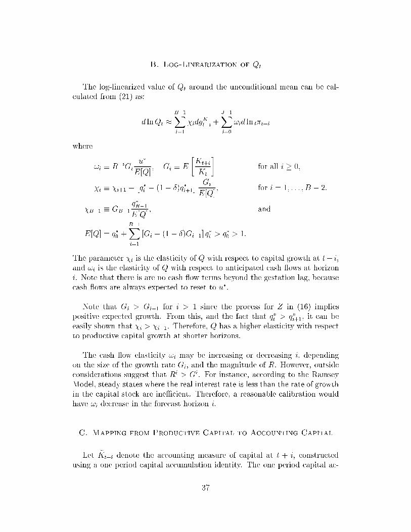
B. Log-Linearization of QtThe log-linearized value of Qt around the un onditional mean an be al- ulated from (21) as:d lnQt � B�1Xi=1 �idgKt+i + J�1Xi=0 !id ln t�t+iwhere !i � R�iGi u�E[Q℄ ; Gi � E �Kt+iKt � for all i � 0;�i � �i+1 + �q�i � (1� Æ)q�i+1� GiE[Q℄ ; for i = 1; : : : ; B � 2;�B�1 � GB�1 q�B�1E[Q℄ ; andE[Q℄ = q�0 + B�1Xi=1 [Gi � (1� Æ)Gi�1℄ q�i > q�0 > 1:The parameter �i is the elasti ity of Q with respe t to apital growth at t+ i,and !i is the elasti ity of Q with respe t to anti ipated ash ows at horizoni. Note that there is are no ash ow terms beyond the gestation lag, be ause ash ows are always expe ted to reset to u�.Note that Gi > Gi�1 for i > 1 sin e the pro ess for Z in (16) impliespositive expe ted growth. From this, and the fa t that q�i > q�i+1, it an beeasily shown that �i > �i+1. Therefore, Q has a higher elasti ity with respe tto produ tive apital growth at shorter horizons.The ash ow elasti ity !i may be in reasing or de reasing i, dependingon the size of the growth rate Gi, and the magnitude of R. However, outside onsiderations suggest that Ri > Gi. For instan e, a ording to the RamseyModel, steady states where the real interest rate is less than the rate of growthin the apital sto k are ineÆ ient. Therefore, a reasonable alibration wouldhave !i de rease in the fore ast horizon i.C. Mapping from Produ tive Capital to A ounting CapitalLet ~Kt+i denote the a ounting measure of apital at t + i, onstru tedusing a one period apital a umulation identity. The one period apital a -37

umulation identity an be iterated ba kwards to yield that~Kt+i+1 = d(L)It+i; where d(L) = 1Xj=0(1� Æ)jLj:Using the arbitrary time to build a ounting in equations (7) to (9), investment an be stated asIt+i = g(L)Kt+J+i; where g(L) = BXj=0 gJ�jLj;and gj � 8><>:�B j = 0�B�j � (1� Æ)�B�j+1 0 < j < B�(1� Æ)�1 j = B :By substitution, these two equations suggest that~Kt+i+1 = m(L)Kt+J+i; where m(L) � d(L)g(L)is the produ t of the two lag polynomials. Performing this multipli ation yieldsthat m(L) = LP�(L); where �(L) = B�1Xj=0 �B�jLj:Therefore, the a ounting measure of apital maps to the produ tive measureby ~Kt+i+1 = �(L)Kt+B+i:The a ounting measure of apital growth is� ln ~Kt+1 = �(L)� lnKt+B:Log-linearizing this around the un onditional expe tation yields that� ln ~Kt+1 � ~�(L)gKt+B;where~�(L) = B�1Xj=0 ~�B�jLj; ~�j = �jGjBPk=1�kGk � 0; and BXj=1 ~�j = 1:38

D. Interpretation of Regression Coeffi ients in Planning LagRegressionGiven the solution for the growth rate of the produ tive apital in (18),dgKt+Bd ~srt�P = 1b d lnEt�P [Zbt+B℄d ~srt�PIn the spe ial ase where the te hnology and labor supply fa tors are indepen-dent, the form of Z in (6) an be used to show thatlnEt�P [Zbt+B℄ = lnEt�P h�ZTt+B�b(1+�)i+ lnEt�P h�ZLt+B�bi ;The standard Solow residual is related to labor-augmenting te hnologi al growthby ~srt�P = � lnZTt�P . Assume that ZT is a random walk, so the Solow residu-als represent permanent sho ks. Taking the onditional expe tation at t� P ,then evaluating the partial derivative with respe t to ~srt�P , one arrives at1b d lnEt�P [Zbt+B℄d ~srt�P = 1b d lnEt�P h�ZTt+B�b(1+�)id ~srt�P = 1 + �:Substituting this into the �rst equation, then substituting and rearranging(29) shows the desired result.E. Spe ifi ation of a Simple RBC Model with Gestation LagsAssume that the so ial planner hooses a onsumption and investment planto maximize the expe ted value of the lifetime utilityU = 1Xj=t �j�tEt [lnCt+j℄ ;subje t to the feasibility onstraint that F �Kt+j; ZTt+jLt+j� = Ct+j + It+j forall j � 0, where F takes the spe i� ation in (1). The evolution of apital isdes ribed by equations (7) to (9) with P = 0, and Lt+j is normalized to onefor all periods. The log of te hnology follows a random walk with a onstantdrift equal to the rate of growth lnG, so that lnZTt+1 = lnG+ lnZTt + t.The optimization problem redu es to the intertemporal �rst order onditionBXj=0 �jgjEt � 1Ct+j � = �BEt �(1� �)�ZTt+BKt+B�� 1Ct+B � ;39

and the onstraint thatCt+s = K1��t+s �ZTt+s�� � BXj=0 gB�jKt+jwhere gj is as de�ned in Appendix C. This nonlinear system links the urrentand future values of the endogenous variables Ct and Kt+B to the set of statevariables (Kt; : : : ; Kt+B�1; Zt). An approximate solution to this system wasobtained by log-linearizing the �rst order onditions around the steady state,then �nding linear feedba k rules for Ct and Kt+B by the method of undeter-mined oeÆ ients, as des ribed in Campbell [1994℄. That is, I solved for the oeÆ ients [���℄ in the following equations:lnCt = B�1Xj=0 � j lnKt+j + � zzt; lnKt+B = B�1Xj=0 �kj lnKt+j + �kzzt;su h that the �rst order onditions were satis�ed, using a numeri al solveralgorithm. Generally there will be many linear solutions of this form thatsatisfy the optimization onditions for a given B > 0. The solution set waslimited to those that implied a stable AR pro ess for apital, i.e., those forwhi h the largest modulus of the roots of the polynomial1�XB�1j=0 �kjLB�jwas outside the unit ir le.The parameters of the model were set to resemble a typi al RBC alibration.The steady state growth fa tor G was set to 1.005, whi h amounts to about2 per ent in annual terms. The dis ount fa tor � was set to G=1:015, whi hensures a risk-free interest rate of 1.5% per quarter. The rate of depre iationÆ was set to 2.5%. For simpli ity, it is assumed that expenditures are spreadevenly throughout the building period, so that �B�j = B�1 for j=0;: : : ;B�1.F. Data Appendix1. Investment and the Capital Sto kA time series was onstru ted for ows of real quarterly aggregate invest-ment from 1946Q4 to 2002Q4 using data from the Federal Reserve Board'sFlow of Funds (FF) and apital sto k estimates from the Bureau of E onomi Analysis (BEA). Ea h quarter's investment was determined by dividing the40

FF �gure for non-�nan ial, non-farm orporations (NFNFC) by the impli itpri e de ator for quarterly nonresidential �xed investment from BEA Table7.6.To obtain the series for the real apital sto k, I iterated the apital a u-mulation identity (7) for a one period time to build. The initial estimate ofthe real apital sto k was determined by dividing the nominal value of nonres-idential �xed apital for non-�nan ial orporations at the end of 1946 by thepri e de ator for the last quarter. In order to minimize the error owing to theestimate of the initial apital sto k, I do not use the apital sto k estimatesprior to 1959Q3. Depre iation rates were al ulated as a weighted average ofthe BEA depre iation rates for stru tures, equipment, and IT apital, withweights set equal to the share of ea h ategory in the nominal value of theaggregate sto k of nonresidential apital for non-�nan ial orporations. Thedepre iation rate for ea h quarter is set to the orresponding annual rate.2. Tax-Adjusted Pri e of CapitalThe tax-adjusted pri e of apital for ea h quarter is al ulated using theequation �pt � pt(1� �t � zt)where pt is the pretax pri e, �t is the investment tax redit, and zt is the presentvalue of depre ation allowan es per dollar of apital. The pretax series is theimpli it pri e de ator for quarterly nonresidential �xed investment from BEATable 7.6. The present value of apital onsumption allowan es (zt) was de-termined using data from DRI on the value of apital onsumption allowan esfor di�erent types of apital, with the share of ea h type in total nominal non-residential investment expenditure as weights. This �gure was then multipliedby the orporate in ome tax rate. Data on the average ITC for equipment andstru tures were obtained from DRI for 1959 to 2002. A weighted average wasthen al ulated using the shares of nominal (nonresidential) �xed investmentfrom BEA Table 5.4. 3. Tobin's QAggregate Tobin's Q is al ulated as the market value of all non-residential�xed apital divided by the repla ement value of non-residential �xed apital,where the repla ement value is al ulated using the previous period's tax-adjusted pri e of aggregate apital:Qt � Vt�pt�1Kt :41

The market value of non-residential �xed apital (Vt) is determined by de-du ting the value of all assets ex ept equipment and nonresidential stru turesfrom the total market value of the �rm. To illustrate, onsider the balan esheet in Table 5, whi h shows the major liabilities and assets of �rms. Assetsin lude the �rm's �nan ial assets (FAt), the present value of the depre iationshields for its existing apital (PVCCAt), inventories (INVt), residential ap-ital (RESKt), and non-residential apital (Qt�pt�1Kt). The olle tive value ofthese assets is equal to the market value of all the laims on these assets: debt(DEBTt) and equity (EQUt). Therefore, to determine an appropriate marketvalue of non-residential apital, one must al ulateVt = EQUt +DEBTt � FINASt � INVt � RESKt � PVCCAt:These omponents were determined from Flow of Funds data for NFNFC, asfollows:EQUt is the FF �gure for the aggregate market value of equity.DEBTt was determined by adding the aggregate book value of non-bond debtliabilities to the aggregate market value of outstanding orporate bonds.The market value of outstanding orporate bonds was estimated usingan algorithm outlined by Hall [2001℄, whi h orre ts the book value ofdebt for hanges in market interest rates. This algorithm is available onHall's website.FINASt is the aggregate book value of �nan ial assets.INVt is the FF �gure for the aggregate repla ement value of inventories.RESKt is the FF �gure for the aggregate repla ement value of all residential apital.PVCCAt was al ulated under the assumption that apital onsumption al-lowan es an be well approximated using a sum-of-years-digits (SYD)method. The stream of allowable depre iation allowan es for ea h quar-ter's expenditure were al ulated using the SYD formula, assuming anaverage asset life of 15 years. To determine the present value of the re-maining onsumption allowan es for any given quarter, I dis ounted thedepre iation allowan es remaining using the BAA orporate rate net ofthe in ome tax rate for orporations.42

4. Rate of Cash FlowCash ows per unit of apital were determined by dividing after tax ash ows by the repla ement value of produ tive apital:�t � ��t�pt�1Kt :After tax ash ows (��t) for ea h quarter were al ulated using FF data forNFNFC, and BEA quarterly aggregates. To determine the ash ow, I addedthe book value of after-tax pro�ts from FF, the value of apital onsumptionallowan es from FF, and net interest payments. Net interest payments were al ulated using BEA data, by dedu ting an estimate of net interest for or-porate farms from the net interest �gure for non-�nan ial orporations. Thisnominal �gure was then adjusted for in ation during the quarter using the rateof in rease in the quarterly GDP de ator for non-�nan ial orporations.

43

Table 1: Sample moments of the tax- orre ted data~gKt+1 ln ~Qt ln (~�t=�p)mean .0111 1.4505 .0628stdev .0029 .5969 .0062 orr(~gKt+1; �) � .5028 .5432 orr(ln ~Qt; �) � � .3659Sample Period: 1959Q3 to 2002Q4 (174 observations). ~gKt+1 rep-resents the growth rate in measured apital, while ~Q and ~� denotethe measured values of Tobin's Q, and the rate of ash ow, re-spe tively.

Table 2: Unit root testsVarian e Ratio (horizon) ~gKt+1 ln ~Qt ln (~�t=�p)VR(5) 2.0822 0.9832 1.3895VR(10) 2.0108 0.7471 1.3904VR(25) 1.2637 0.5910 0.8012VR(50) 0.5612 0.5182 0.2500VR(100) 0.1870 0.1230 0.1596ADF T-Statisti -2.9487z -1.8442 -3.8938#Signi� an e Levels: z5%; #1%. Sample Period: 1959Q3 to 2002Q4 (174observations). VR(n) denotes the value of the varian e ratio at a horizonof n periods. The ADF T-Statisti is for an augmented Di key-Fuller testwhere the null is the existen e of a unit root.44

Table 3: Planning Horizon Estimates by OLSMeasured Capital Growth on Lags of Puri�ed Solow Residuallag di ser lag di ser0 -.0052 .0203 8 .0351 .0168z1 .0026 .0246 9 .0282 .0129z2 .0092 .0222 10 .0275 .0133z3 .0195 .0171 11 .0232 .01464 .0269 .0143y 12 .0171 .01585 .0328 .0148z 13 .0201 .01446 .0349 .0169z 14 .0146 .01347 .0377 .0172z onst .0101 .0008#Sele ted Tests Using Estimated CoeÆ ientssum lags oef ser CIb 900 to 10 .2492 .1551 -.0231,.62144 to 10 .2463 .0993 .0480,.44084 to 7 .1324 .0575 .0105,.26030 to 3 .0261 .0795 -.1001,.1896(4 to 7) - (0 to 3) .1063 .0532 -.0132,.1873Signi� an e Levels: y10%, z5%, #1%; �R2 = .0068; dw = .0680. Sample Pe-riod: 1965Q3 to 2002Q2 (150 observations). Standard errors are robust forheteroskedasti ity and auto orrelation (Newey-West maximum lag = 15).

45

Table 4: Building Horizon Estimates by Instrumental VariablesMeasured Capital Growth on Instrumented Leads of Impli it Produ tive Capital Growthlead hi ser CIb 90 R2p lead hi ser CIb 90 R2p1 .0706 .1282 -.0037,.4323 .1186 7 .2458 .0747# .2482,.6667# .11372 .1372 .1466 .0670,.5651z .1060 8 .2201 .0698# .2014,.6304# .11833 .0706 .1239 -.0443,.3716 .0992 9 .1049 .1396 -.0228,.2956 .08514 .1056 .1076 .0094,.3917y .1171 10 .1092 .1131 -.0860,.2833 .09525 .2314 .1482 .2182,.6620# .0843 11 .0759 .1112 -.1375,.2391 .11626 .2539 .1101z .2390,.6845# .1208 12 -.0088 .1089 -.3566,.0771 .1040Sele ted Tests Using Estimated CoeÆ ientslinear ombination oef ser CIb 90h1 + : : :+ h8 1.3352 .5886 1.2942, 3.0308h1 + : : :+ h9 1.4401 .5989 1.3643, 3.3450h1 + : : :+ h10 1.5493 .5762 1.4664, 3.6412h1 + : : :+ h11 1.6251 .5598 1.5424, 3.7840Signi� an e Levels: y10%, z5%, #1%. Sample Period: 1965Q3 to 2002Q2 (150 observations). In-struments (28): gHt ; : : : ; gHt�13, ~gKt ; : : : ; ~gKt�13. IV standard errors are robust for heteroskedasti ityand auto orrelation (Newey-West maximum lag = 15). R2p is the \partial R2" outlined in Shea[1997℄, whi h measures the squared orrelation between the portion of the regressor that is or-thogonal to the other regressors, and the portion of the �tted regressor that is orthogonal to theother �tted regressors. The overidentifying restri tions annot be reje ted at 1% signi� an e, after orre ting for small-sample bias. Bias- orre ted intervals were onstru ted using 50,000 bootstraprepli ations, with re-sampling in blo ks of 12 adja ent observations. An in luded onstant is notreported.

46

t t+P t+P+i t+J

Capital is ProductiveBuilding BeginsCapital Planned

P "planning" periods B "building" periods

... ...

PSfrag repla ements�B �B�i

Figure 1: Time s ale depi tion of the investment pro ess with gestation lags.

DemandAnticipated

Ex ante Supply

"Ex ante" Market

usercostPSfrag repla ements u�u0Kt+J Kt+J K

QUASI

"Ex post" Market

Ex ante Supply

user

DemandRealized

Ex post Supply

RENT

costPSfrag repla ements u�u0Kt+J Kt+J KFigure 2: Diagram of equilibrium in the ex ante and ex post apital servi esmarket.47

0 .005 .01 .015 .02

1960q1

1965q1

1970q1

1975q1

1980q1

1985q1

1990q1

1995q1

2000q1

2005q1

Quarter

Figure3:Plotofmeasured apitalgrowth.

0 .01 .02 .03 .04 .05 .06 .07 .08 .09 .1

1960q1

1965q1

1970q1

1975q1

1980q1

1985q1

1990q1

1995q1

2000q1

2005q1

Quarter

Cash F

lows

Tax C

orrected Cash F

lows

Figure4:Plotoftherateof ash ow.

0 1 2 3 4

1960q1

1965q1

1970q1

1975q1

1980q1

1985q1

1990q1

1995q1

2000q1

2005q1

Quarter

QT

ax Corrected Q

Figure5:PlotofTobin'sQ.

−1 −.5 0 .5 1 1.5

1960q1

1965q1

1970q1

1975q1

1980q1

1985q1

1990q1

1995q1

2000q1

2005q1

Quarter

Log of QF

itted Trend

Figure6:LogofTobin'sQand�ttedtrend

−.04 −.02 0 .02 .04

1960q1

1965q1

1970q1

1975q1

1980q1

1985q1

1990q1

1995q1

2000q1

2005q1

Quarter

Cleaned S

olow R

esidualsG

rowth in Labor H

ours

Figure7:Hoursgrowthandpuri�edSolowresiduals.

−0.50 0.00 0.50 1.00Autocorrelations of gk

010

2030

LagB

artlett’s formula for M

A(q) 90%

confidence bands

Figure8:Correlogramofmeasured ap-italgrowth.

48

0 10 20 30 40 50 60 70 80 90 1000

0.1

0.2

0.3

0.4

0.5

0.6

0.7

0.8

0.9

1

Quarters

Per

cent

age

TTB = 1TTB = 2TTB = 3TTB = 4TTB = 5TTB = 6TTB = 7TTB = 8TTB = 9Figure 9: Dynami response of the measured apital sto k to a permanent oneper entage point te hnology sho k in alibrated RBC models featuring timeto build of in reasing duration.

49

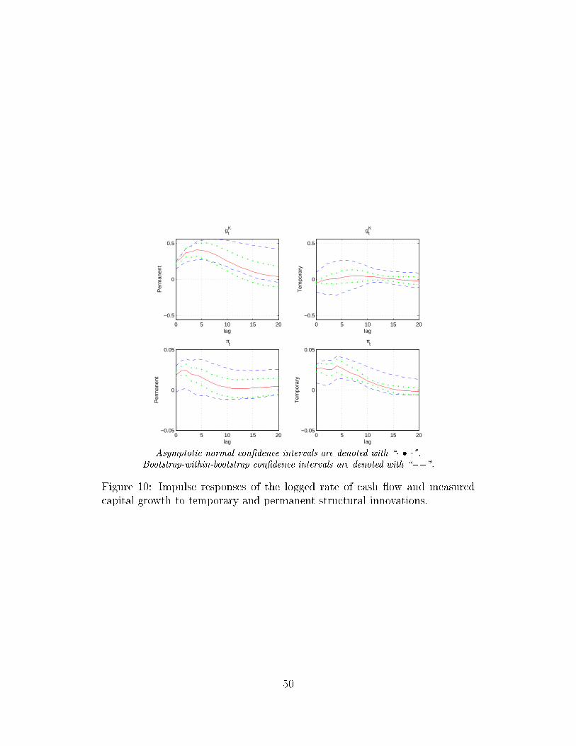
0 5 10 15 20

−0.5

0

0.5

lag

gKt

Per

man

ent

0 5 10 15 20

−0.5

0

0.5

lag

gKt

Tem

pora

ry

0 5 10 15 20−0.05

0

0.05

lag

πt

Per

man

ent

0 5 10 15 20−0.05

0

0.05

lag

πt

Tem

pora

ry

Asymptoti normal on�den e intervals are denoted with \� � �".Bootstrap-within-bootstrap on�den e intervals are denoted with \��".Figure 10: Impulse responses of the logged rate of ash ow and measured apital growth to temporary and permanent stru tural innovations.

50

0 5 10 15 20−0.5

0

0.5

lag

gKt

Per

man

ent

0 5 10 15 20−0.5

0

0.5

lag

gKt

Tem

pora

ry

0 5 10 15 20

−0.1

−0.05

0

0.05

0.1

lag

Qt

Per

man

ent

0 5 10 15 20

−0.1

−0.05

0

0.05

0.1

lag

Qt

Tem

pora

ry

Asymptoti normal on�den e intervals are denoted with \� � �".Bootstrap-within-bootstrap on�den e intervals are denoted with \��".Figure 11: Impulse response of logged Tobin's Q and measured apital growthto temporary and permanent stru tural innovations.

51

5 10 15 20

−0.1

−0.05

0

0.05

0.1

lag

d gKt

Per

man

ent

5 10 15 20

−0.1

−0.05

0

0.05

0.1

lag

d gKt

Tem

pora

ry

5 10 15 20−0.01

−0.005

0

0.005

0.01

lag

d πt

Per

man

ent

5 10 15 20−0.01

−0.005

0

0.005

0.01

lag

d πt

Tem

pora

ry

Asymptoti normal on�den e intervals are denoted with \� � �".Bootstrap-within-bootstrap on�den e intervals are denoted with \��".Figure 12: First-di�eren e of the impulse responses of the logged rate of ash ow and measured apital to temporary and permanent stru tural innovations.

52

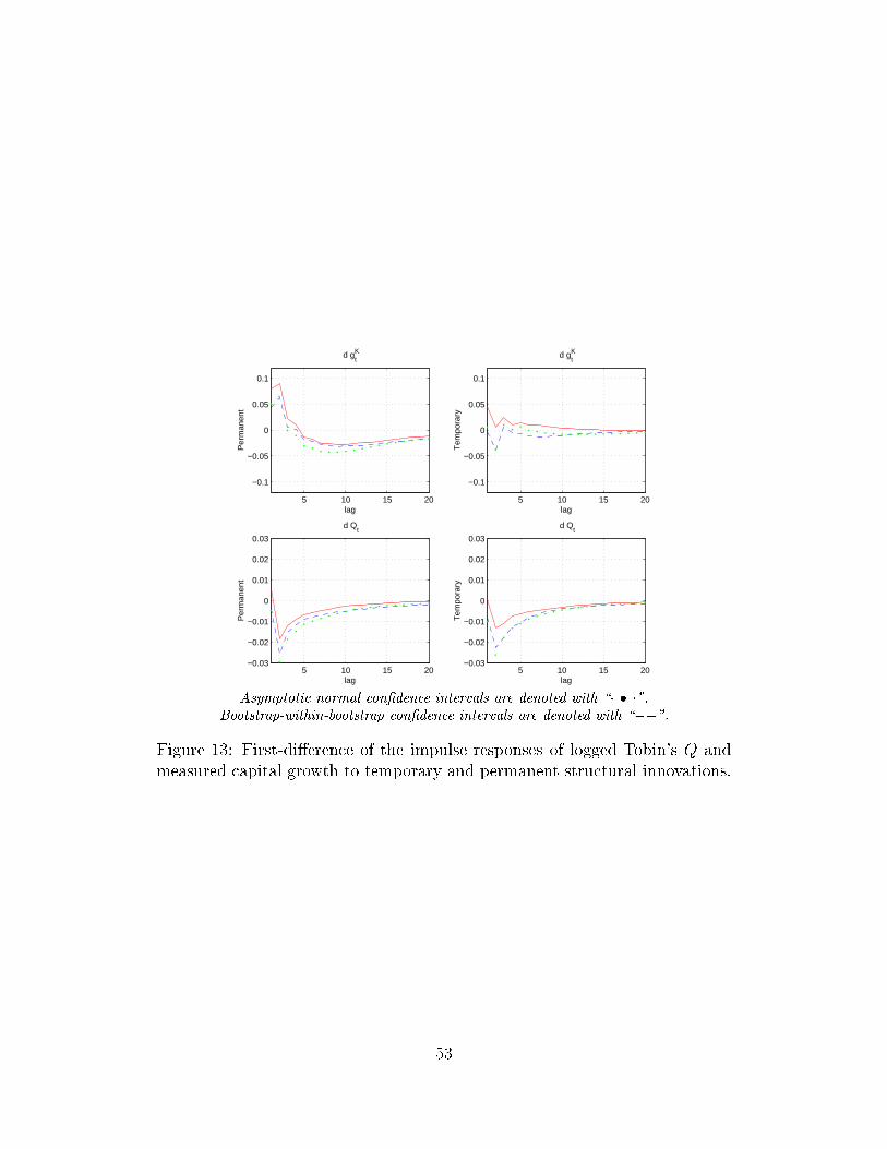
5 10 15 20

−0.1

−0.05

0

0.05

0.1

lag

d gKt

Per

man

ent

5 10 15 20

−0.1

−0.05

0

0.05

0.1

lag

d gKt

Tem

pora

ry

5 10 15 20−0.03

−0.02

−0.01

0

0.01

0.02

0.03

lag

d Qt

Per

man

ent

5 10 15 20−0.03

−0.02

−0.01

0

0.01

0.02

0.03

lag

d Qt

Tem

pora

ry

Asymptoti normal on�den e intervals are denoted with \� � �".Bootstrap-within-bootstrap on�den e intervals are denoted with \��".Figure 13: First-di�eren e of the impulse responses of logged Tobin's Q andmeasured apital growth to temporary and permanent stru tural innovations.

53

5 10 15 20−0.3

−0.2

−0.1

0

0.1

0.2

0.3

lag

After impact gKt

Per

man

ent

5 10 15 20−0.3

−0.2

−0.1

0

0.1

0.2

0.3

lag

After impact gKt

Tem

pora

ry

5 10 15 20−0.04

−0.02

0

0.02

0.04

lag

After impact πt

Per

man

ent

5 10 15 20−0.04

−0.02

0

0.02

0.04

lag

After impact πt

Tem

pora

ry

Asymptoti normal on�den e intervals are denoted with \� � �".Bootstrap-within-bootstrap on�den e intervals are denoted with \��".Figure 14: Net-of-impa t impulse response of the logged rate of ash ow andmeasured apital growth to temporary and permanent stru tural innovations.

54

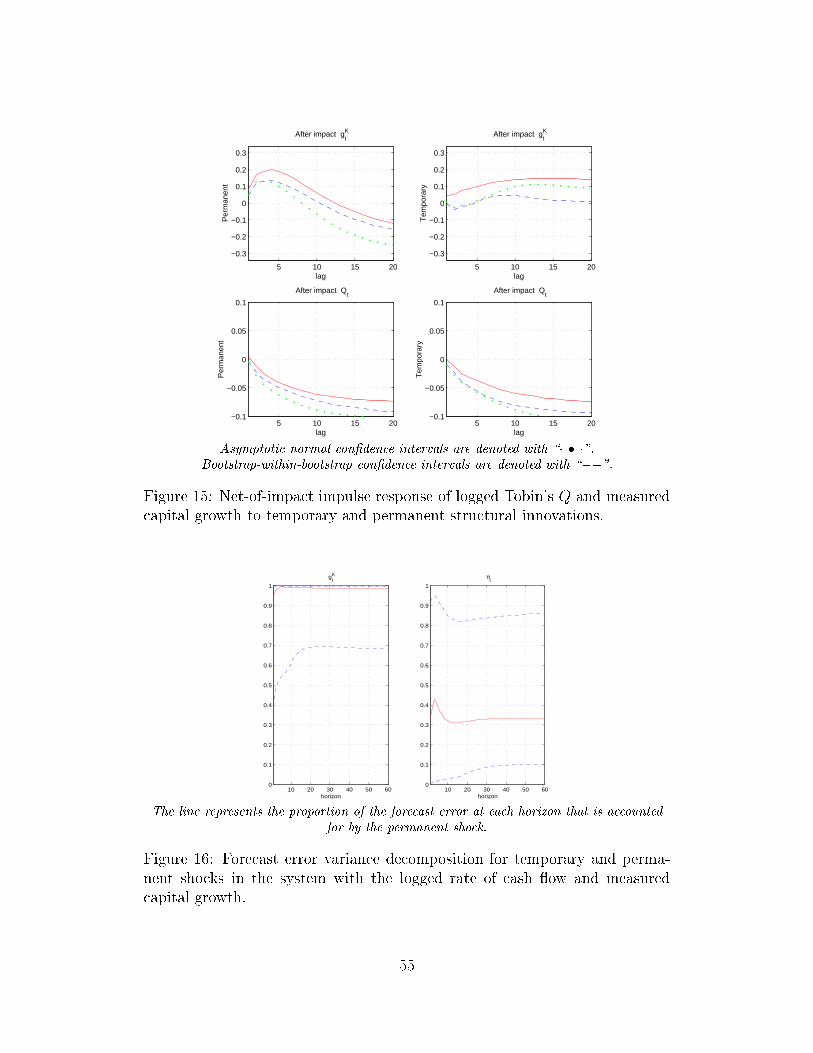
5 10 15 20

−0.3

−0.2

−0.1

0

0.1

0.2

0.3

lag

After impact gKt

Per

man

ent

5 10 15 20

−0.3

−0.2

−0.1

0

0.1

0.2

0.3

lag

After impact gKt

Tem

pora

ry5 10 15 20

−0.1

−0.05

0

0.05

0.1

lag

After impact Qt

Per

man

ent

5 10 15 20−0.1

−0.05

0

0.05

0.1

lag

After impact Qt

Tem

pora

ry

Asymptoti normal on�den e intervals are denoted with \� � �".Bootstrap-within-bootstrap on�den e intervals are denoted with \��".Figure 15: Net-of-impa t impulse response of logged Tobin's Q and measured apital growth to temporary and permanent stru tural innovations.

10 20 30 40 50 600

0.1

0.2

0.3

0.4

0.5

0.6

0.7

0.8

0.9

1

gKt

horizon10 20 30 40 50 60

0

0.1

0.2

0.3

0.4

0.5

0.6

0.7

0.8

0.9

1

πt

horizonThe line represents the proportion of the fore ast error at ea h horizon that is a ountedfor by the permanent sho k.Figure 16: Fore ast error varian e de omposition for temporary and perma-nent sho ks in the system with the logged rate of ash ow and measured apital growth. 55

10 20 30 40 50 600

0.1

0.2

0.3

0.4

0.5

0.6

0.7

0.8

0.9

1

gKt

horizon10 20 30 40 50 60

0

0.1

0.2

0.3

0.4

0.5

0.6

0.7

0.8

0.9

1

Qt

horizonThe line represents the proportion of the fore ast error at ea h horizon that is a ountedfor by the permanent sho k.Figure 17: Fore ast error varian e de omposition for temporary and perma-nent sho ks in the system with logged Tobin's Q and measured apital growth.

0 5 10 15 20

−4

−2

0

2

4

lag

gYt

Per

man

ent

0 5 10 15 20

−4

−2

0

2

4

lag

gYt

Tem

pora

ry

0 5 10 15 20

−1.5

−1

−0.5

0

0.5

1

1.5

lag

rt

Per

man

ent

0 5 10 15 20

−1.5

−1

−0.5

0

0.5

1

1.5

lag

rt

Tem

pora

ry

Asymptoti normal on�den e intervals are denoted with \� � �".Bootstrap-within-bootstrap on�den e intervals are denoted with \��".Figure 18: Impulse response of output growth and the real interest rate totemporary and permanent stru tural innovations.56

0 5 10 15 20

−1

−0.5

0

0.5

1

gKt

Per

man

ent

0 5 10 15 20

−1

−0.5

0

0.5

1

gKt

Tem

pora

ry

0 5 10 15 20−0.2

−0.1

0

0.1

0.2

πt

Per

man

ent

0 5 10 15 20−0.2

−0.1

0

0.1

0.2

πt

Tem

pora

ry

0 5 10 15 20

−0.05

0

0.05

Qt

Per

man

ent

0 5 10 15 20

−0.05

0

0.05

Qt

Tem

pora

ryAsymptoti normal on�den e intervals are denoted with \� � �".Bootstrap-within-bootstrap on�den e intervals are denoted with \��".Figure 19: Impulse response of measured apital growth, the logged rate of ash ow and logged Tobin's Q to separately-identi�ed temporary and perma-nent stru tural innovations.

57

Table 5: Stylized Balan e SheetAssets Liabilities + EquityFINASt DEBTtPVCCAtINVtRESKtQt�pt�1Kt EQUtTotal Market Value Total Market Value

58

Referen esAbel, Andrew B., Eberly, Jani e C. \A Uni�ed Model of Investment UnderUn ertainty." The Ameri an E onomi Review, 1994, 84(5), 1369-1384.Abel, Andrew B., Eberly, Jani e C. \Q Theory Without Adjustment Costsand Cash Flow E�e ts Without Finan ing Constraints." Unpublishedmanus ript, 2002.Altug, Sumru. \Time-to-Build, Delivery Lags, and the Equilibrium Pri ingof Capital Goods." Journal of Money, Credit, and Banking, 1993, 25(3),301-319.Barnett, Steven, Sakellaris, Plutar hos. \Non-linear Response of Firm Invest-ment to Q: Testing a Model of Convex and Non- onvex Adjustment Costs"."Journal of Monetary E onomi s, 1998, 42(2), 261-288.Basu, Susanto, Fernald, John G., Shapiro, Matthew D. \Produ tivity Growthin the 1990s: Te hnology, Utilization, or Adjustment?" Carnegie-Ro hesterSeries on Publi Poli y, 2000.Berndt, Ernst R., Fuss, Melvin A. \Produ tivity measurement with adjust-ments for variations in apa ity utilization and other forms of temporaryequilibrium." Journal of E onometri s, 1986, 33(1), 7-29.Blan hard, Olivier Jean, Quah, Danny. \The Dynami E�e ts of AggregateDemand and Supply Disturban es." The Ameri an E onomi Review, 1989,79(4), 655-673.Bound, John, Jaeger, David, and Baker, Regina. \Problems with InstrumentalVariables Estimation When the Correlation between the Instruments andthe Endogeneous Explanatory Variable is Weak." Journal of the Ameri anStatisti al Asso iation, 1995, 90, 443-450.Caballero, Ri ardo J.. \Small Sample Bias and Adjustment Costs." Review ofE onomi s and Statisti s, 1994, 76(1), 52-58.Caballero, Ri ardo J.. \Aggregate Investment." In: Taylor, John and Mi haelWoodford (Eds) Handbook of Ma roe onomi s V1, 1999, 813-862.Caballero, Ri ardo J., Engel, Eduardo M.R.A., Haltiwanger, John C.. \Plant-Level Adjustment and Aggregate Investment Dynami s." Brookings Paperson E onomi A tivity, 1995, 1995(2), 1-51.Caballero, Ri ardo J., Engel, Eduardo M.R.A.. \Explaining Investment Dy-nami s in U.S. Manufa turing: a Generalized s,S approa h." E onometri a,1999, 67(4), 783-826. 59

Caballero, Ri ardo J., Leahy, John V.. \Fixed Costs: The Demise of Marginalq." NBER working paper w5508, 1996.Campbell, John Y..\Inspe ting the Me hanism: An Analyti al Approa h tothe Sto hasti Growth Model." Journal of Monetary E onomi s, 1994, 33(3),463-506.Chang, Pau-Li., Sakata, Shini hi.. \A Misspe i� ation-Robust Impulse Re-sponse Estimator." Unpublished manus ript, 2003.Christiano, Lawren e J., Todd, Ri hard M.. \Time to Plan and AggregateFlu tuations." Federal Reserve Bank of Minneapolis Quarterly Review,1995, 20(1), 14-27.Co hrane, John H. \How Big is the Random Walk in GNP?" Journal of Po-liti al E onomy, 1988, 96(5), 893-920.Doms, Mark, Dunne, Timothy. \Capital Adjustment Patterns in Manufa tur-ing Plants." Review of E onomi Dynami s, 1998, 1(2), 409-429.Er eg, Christopher J., Levin, Andrew T. \Optimal Monetary Poli y withDurable and Non-Durable Goods." Working Paper, Board of Governors ofthe Federal Reserve, 2003.Eri kson, Timothy, Whited, Toni M. \Measurement Error and the Relation-ship between Investment and q." Journal of Politi al E onomy, 2000, 108(5),1027-1057.Fazzari, Steven R., Hubbard, R. Glenn, Peterson, Bru e C. \Finan ing Con-straints and Corporate Investment." Brookings Papers on E onomi A tiv-ity, 1988, 1988(1), 141-195.Hall, Robert E. \The Sto k Market and Capital A umulation." Ameri anE onomi Review, 2001, 91, 1185-1202.Hayashi, Fumio. \Tobin's Marginal q and Average q: A Neo lassi al Interpre-tation." E onometri a, 1982, 50(1), 213-224.Hulten, Charles R. \Produ tivity hange, apa ity utilization, and the sour esof eÆ ien y growth." Journal of E onometri s, 1986, 33(1), 31-50.Jorgenson, Dale W., Yun, Kun-Young. Tax Reform and the Cost of Capital,Oxford: Clarendon Press, 1991.Jorgenson, Dale W., Stephenson, James A. \The Time Stru ture of InvestmentBehavior in United States Manufa turing, 1947-1960." Review of E onomi sand Statisti s, 1967, 49, 16-27.. 60

Kilian, Lutz. \Small-Sample Con�den e Intervals for Impulse Response Fun -tions." The Review of E onomi s and Statisti s, 1998, 80(2), 218-230.Kimball, Miles S. \Q-Theory and Real Business Cy le Analyti s." Universityof Mi higan Working Paper, 2003.King, Robert G., Plosser, Charles I., and Rebelo, Sergio T. \Produ tion,Growth and Business Cy les." Journal of Monetary E onomi s, 195-232.Koeva, Petya. \The Fa ts about Time to Build." IMF Working Paper 00/138,2000.Kydland, Finn E., Pres ott, Edward C.. \Time to Build and Aggregate Flu -tuations." E onometri a, 1982, 50(6),1345-1371.Krainer, Robert E.. \The Time Pro�le of Capital A umulation in the Auto-mobile Industry." Journal of Politi al E onomy, 1968, 76, 1049-57.Laitner, John P., and Stolyarov, Dmitriy L.. \Te hnologi al Change and theSto k Market." Ameri an E onomi Review, 2003, 93(4), 1240-1267.L�utkepohl, Helmut. Introdu tion to Multiple Time Series Analysis, New York:Springer-Verlag, 1993.Mayer, Thomas. \Plant and Equipment Lead Times." Journal of Business,1960, 33, 127-132.Majd, Saman, Pindy k, Robert. \Time to Build, Option Value, and InvestmentDe isions." Journal of Finan ial E onomi s, 1987, 18, 7-27.M Grattan, Ellen R, Pres ott, Edward C. \Taxes, Regulations, and the Valueof U.S. Corporations: A General Equilibrium Analysis" Federal ReserveBank of Minneapolis Resear h Sta� Report 309, 2002.Millar, Jonathan. \Gestation Lags and the Relationship Between Investmentand Q in Regressions" Dissertation Chapter, University of Mi higan, 2005.Newey W., and West, K. \A Simple, Positive Semi-De�nite, Heteros edasti ityand Auto orrelation Consistent Covarian e Matrix." E onometri a, 1987,55, 703-708.Romer, David. Advan ed Ma roe onomi s, New York: M Graw-Hill, 1996.Sargent, Thomas J. Dynami Ma roe onomi Theory, Cambridge, MA: Har-vard University Press, 1987.Shapiro, Matthew D. \The Dynami Demand for Capital and Labor." Quar-terly Journal of E onomi s, 1986, 101(3), 513-542.61

Shapiro, Matthew D., Watson, Mark W. \Sour es of Business Cy le Flu tua-tions." NBER Ma ro Annual, 1988, 3, 111-148.Shea, John. \Instrument Relevan e in Multivariate Linear Models: A SimpleMeasure." Review of E onomi s and Statisti s, 1997, 79(2), 348-352.Sto k, James H., Watson, Mark W. \Business Cy le Flu tuations in USMa roe onomi Time Series." In: Taylor, John and Mi hael Woodford (Eds)Handbook of Ma roe onomi s V1, 1999, 3-64.Sto k, James H., Wright, Jonathan H., and Yogo, Motohiro. \A Survey ofWeak Instruments and Weak Identi� ation in General Method of Moments."Journal of Business and E onomi Statisti s, 2002, 20(4), 518-529.Summers, Lawren e H. \Taxation and Corporate Investment: A q-TheoryApproa h." Brookings Papers on E onomi A tivity, 1981, 1981(1), 67-127.Thomas, Julia K. \Is Lumpy Investment Relevant for the Business Cy le?"Journal of Politi al E onomy, 2002, 110(3), 508-534.Whelan, Karl. \A Guide to the Use of Chain Aggregated NIPA Data." FEDSworking paper, 2000-35.Wooldridge, Je�rey M. E onometri Analysis of Cross Se tion and Panel Data,Cambridge: The MIT Press, 2002.\Fixed Reprodu ible Tangible Wealth of the United States, 1925-94," Bureauof E onomi Analysis, August 1999.

62