geostatistical analysis of soil texture fractions on the ... · pdf file175 soil & water...

173

Soil & Water Res., 6, 2011 (4): 173–189

Geostatistical Analysis of Soil Texture Fractions on the Field Scale

Masoomeh DELBARI1, Peyman AFRASIAB1 and Willibald LOISKANDL2

1Department of Water Engineering, Faculty of Agriculture, University of Zabol, Zabol, Iran; 2Institute of Hydraulics and Rural Water Management, Department of Water, Atmosphere

and Environment, University of Natural Resources and Applied Life Sciences, Vienna, Austria

Abstract: Geostatistical estimation methods including ordinary kriging (OK), lognormal ordinary kriging (LOK), cokriging (COK), and indicator kriging (IK) are compared for the purposes of prediction and, in particular, uncertainty assessment of the soil texture fractions, i.e. sand, silt, and clay proportions, in an erosion experimental field in Lower Austria. The soil samples were taken on 136 sites, about 30-m apart. The validation technique was cross-validation, and the comparison criteria were the mean bias error (MBE) and root mean squared error (RMSE). Statistical analysis revealed that the sand content is positively skewed, thus persuading us to use LOK for the estimation. COK was also used due to a good negative correlation seen between the texture fractions. The autocorrelation analysis showed that the soil texture fractions in the study area are strongly to moderately correlated in space. Cross-validation indicated that COK is the most accurate method for estimating the silt and clay contents; RMSE equalling to 3.17% and 1.85%, respectively. For the sand content, IK with RMSE (12%) slightly smaller than COK (RMSE = 14%) was the best esti-mation method. However, COK maps presented the true variability of the soil texture fractions much better than the other approaches, i.e. they achieved the smallest smoothness. Regarding the local uncertainty, the estimation variance maps produced by OK, LOK, and COK methods similarly indicated that the lowest uncertainty occurred near the data locations, and that the highest uncertainty was seen in the areas of sparse sampling. The uncertainty, however, varied much less across the study area compared to conditional variance for IK. The IK conditional variance maps showed, in contrast, some relations to the data values. The estimation uncertainty needs to be evaluated for the incorporation into the risk analysis in the soil management.

Keywords: estimation uncertainty; kriging; prediction; soil texture fractions; spatial variability

In recent years, an increasing number of soil phys-ical and chemical process models and pedotransfer functions were developed for different purposes such as modelling the water movement and solute transport in soil (Gupta & Larson 1979; Rawls et al. 1982) or assessing soil erosion sensivity (Mor-gan et al. 1998). A key parameter used in many soil process models and pedotransfer functions is soil texture fraction, i.e. sand, silt and clay percent-ages, which should be quantified accurately on the point scale. As in many cases sparse sampling is only available, some sort of spatial interpolation is required to produce a more detailed picture of

the soil texture fractions. Whatever interpolation method is used, there is always some uncertainty attached to the estimates. These uncertainties cannot be neglected and need to be evaluated to assess the reliability of the estimates and the risk involved in any related decision-making process.

Geostatistics as a set of tools for spatial char-acterisation of the soil properties and estimation with incorporating the spatial continuity behaviour of the soil data into the estimation process has been increasingly used in the soil science over the last two decades (Trangmar et al. 1985; Cam-bardella et al. 1994; Gonzalez & Zak 1994;

174

Soil & Water Res., 6, 2011 (4): 173–189

Goovaerts 1998; Gaston et al. 2001, López -Granados et al. 2002; Nogueira et al. 2002; Ersahin & Brohi 2006; Delbari 2007). The most popular geostatistical interpolation method, also known as the best linear unbiased estimator (BLUE), is ordinary kriging (OK) (Journel & Huijbregts 1978; Isaaks & Srivastava 1989). OK has an extensive application in the soil science (Burgess & Webster 1980). Conventional classification methods of soil properties mapping indicate higher precision when combined with OK (Voltz et al. 1997). However, OK tends to smooth out the details, i.e. small values are overestimated while high values are underestimated. The smoothing effect of OK is a serious problem especially when the detection of extreme values is the main concern of the problem at hand. Therefore, OK is no longer suitable when dealing with the data of highly skewed distribution. On the other hand many soil properties in earth sciences do not follow a normal distribution due to the existence of few very small or very large values. These extreme values may affect summary statistics, e.g. the mean or variance, or spatial correlation measures of the data, e.g. the semivariogram. There are different ways to handle such extreme values. One way is to remove the extreme values from the data if, of course, their erroneousness is declared. The second way is to classify them into a separate population. This is, however, conditional on the density of the available data to allow the deviation of the reliable statistics for each subset (Goovaerts 1997). The other way is to transform the data us-ing some transformation function, e.g. logarithmic transformation applied for a positively skewed histogram (Saito & Goovaerts 2000), since many phenomena in earth science are log-normally dis-tributed. More generally, indicator kriging (IK) is a non-parametric (distribution-free) counterpart of OK, which can overcome the smoothing effect of OK (Journel 1983). IK is also a useful method for presenting the connectivity of extreme values in a spatial field (Goovaerts 1997).

Soil information is usually multivariate. Cokriging (COK) is a multivariate extension of OK to the situ-ations where one or more secondary variables are spatially cross-correlated with the primary variable. In such cases, the readily available secondary infor-mation is used to improve the quality of soil prop-erties estimates (Yates & Warrick 1987; Zhang et al. 1992, 1997; Vaughan et al. 1995; Gotway & Hartford 1996; Juang & Lee 1998). For example, Ersahin (2003) compared OK and COK for estimat-

ing the infiltration rate. He found that COK could estimate the infiltration rate more accurately than OK when the infiltration rate measurements are limited and some well-correlated secondary variable like bulk density is available. Another study conducted by Bishop and McBratney (2001) showed that in the presence of secondary information with a high or even poor correlation with the main attribute, OK is no longer suggested and hybrid methods such as kriging with external drift (KED) will result in a more precise estimation. Other researchers also suggest that the denser and less expensive auxiliary data, e.g. aerial photographs could be used to improve the prediction accuracy of the soil properties from the sparse information obtained through soil sur-veys (Kerry & Oliver 2003; López-Granados et al. 2005). There are different case studies in which various kriging methods were compared. For ex-ample, in a study conducted by Triantafilis et al. (2001), ordinary kriging, regression kriging, three-dimensional kriging, and cokriging were compared for predicting soil salinity. Lopez-Granados et al. (2002) examined the spatial patterns of seven soil chemical properties and texture fractions over two fields in southern Spain for the implementation of a site-specific fertilisation practice. Odeh et al. (2003) applied OK and COK to estimate soil particle-size fractions.

In spite of the main application of geostatistics for mapping the soil properties in soil science (Goova-erts 1999), it is increasingly used for assessing the uncertainty attached to the estimates. A unique feature of OK is to produce an estimation variance corresponding to each estimate, which can provide a measure of confidence on the modelled surface (Goovaerts 1997). The OK variance depends, how-ever, on the data arrangement and model of spatial continuity only and is independent of the data values (Lloyd & Atkinson 1999). Therefore, except under homoscedaticity and normality of the distribution of the estimation errors, kriging variance cannot be used as a reliable measure of the estimation uncertainty (Goovaerts 1997). IK, in contrast, can be used for modelling local uncertainty by considering the val-ues of actual data in addition to their configuration (Goovaerts 1997). Instead of estimating a unique value for an unsampled location, IK estimates a cu-mulative distribution function (cdf ) corresponding to each location, which, after being post processed, different measures of local uncertainty such as con-ditional variance can be obtained (Goovaerts et al. 1997; Mohammadi et al. 1997).

175

Soil & Water Res., 6, 2011 (4): 173–189

In this study, the objectives are to predict the spatial distribution of soil texture fractions and to assess the uncertainty attached to the estimates, in particular in an erosion experiment in Lower Austria. For this purpose, the feasibility of using different kriging methods such as OK, LOK, COK, and IK is examined.

MATERIALS AND METHODS

Study area and data set

This study is conducted on a 18 ha hilly slope field (16°34' longitude and 48°34' latitude) located in a 40 ha agriculturally used watershed (Figure 1a). The field is located in Lower Austria, roughly 40 km northeast of Austria’s capital Vienna and approxi-mately 25 to 30 km from the Czech and the Slovak boarders. Geologically, the northern part of the so-called Viennese basin is alluvial deposits (Molasse zone, Zötl 1997). The landscape is characterised by gently to fairly steep slopes (5–20%). The mean annual temperature in 1994–2001 was about 9.6°C while the average annual precipitation is about 665 mm. The samples were collected from the surface layer (0–10 cm) in July 2002. A total of 136 soil samples were taken on an almost regular grid, about 30 m apart. Fine soil texture fractions (sand, silt and clay) were determined from the grain size distribution obtained through the sieving and pipette methods. Soil bulk density was also measured; the average value was 1.38 g/cm3. The location map of the sampling points is shown in Figure 1b.

Geostatistical analysis

Geostatistical analysis usually begins with in-vestigating the spatial continuity between the observations. The semivariogram and cross-sem-ivariogram functions describe the spatial (cross) correlation between the data values (Isaaks & Srivastava 1989). The experimental semivari-ogram and cross-semivariogram are calculated using the following equation:

(1)

where:g*

vw – experimental semivariogram when v = w and cross-semivariogram when v ≠ w

N(h) – number of pairs of random variables Zv(xi) and Zw(xi) at a given separation distance h

A best fit theoretical model of (cross) semivari-ogram is then used in kriging system to predict the spatial distribution of the soil texture fractions. The experimental semivariogram calculation and fitting models are performed using software pack-age GS+ (Robertson 2000).

Ordinary kriging

In ordinary kriging (OK, Isaaks & Srivastava 1989), the values at the unsampled locations are

X (m)

Y (m

)

(b) (a)

AUSTRIA

GERMANY

ITALY

Lower Austria

0 50 100 km

N

Forest

Figure 1. Geographical locatio of the study area (a) and soil sampling sites (b)

)(

1

* )()()()()(2

1)(γhN

iwiwvivvw xZhxZxZhxZ

hNh

)(

1

* )()()()()(2

1)(γhN

iwiwvivvw xZhxZxZhxZ

hNh

176

Soil & Water Res., 6, 2011 (4): 173–189

estimate of a property in real space (Patriarche et al. 2005).

CokrigingThe cokriging (COK) estimator Z*

v(x0) at the un-sampled location x0, assuming there is one auxiliary variable Zw cross-correlated with the main vari-able Zv, is given as (Isaaks & Srivastava 1989):

(5)

where: ai, bj – weights assigned to the known values of the primary

and secondary variables Zv and Zw, respectivelyn, m – numbers of primary and secondary observations

Like for OK, to obtain an unbiased estimate of the primary variable, the sum of weights ai should be unity while the sum of weights bj should be zero and the COK estimation variance is minimised (Goovaerts 1997).

Indicator kriging Indicator kriging (IK) is based on the coding of

the random function Z(x) into a set of K indica-tor random functions I(x, zk) corresponding to different cutoffs zk:

(6)

After transforming the observed data to a new set of indicator variables, the experimental semi-variogram is calculated for every set of indicators at each cutoff zk as:

(7)

where:gI

*(h) – indicator experimental semivariogramN(h) – number of pairs of indicator transforms I(xi; zk)

and I(xi+h; zk) at locations xi and xi+h, respec-tively,

h – separation distance vector

The conditional cumulative distribution func-tion (ccdf ) at each unsampled location, e.g. x0, is then obtained by the IK estimator:

(8)

determined by a linear weighted moving averaging of the values at the sampled locations, i.e.:

(2)

where:Z*(x0) – estimated value of the variable of interest at the

unsampled location x0li – weight assigned to the known value of the vari-

able at location xi determined based on a semi-variogram model

n – number of neighbouring observations

Allocating weights to the known locations is done in such a way that they sum to unity to provide an unbiased estimation (E [Z*(x0) −Z(x0)] = 0). By minimising the kriging estimation error vari-ance, the unknown weights are found by solving the following system of (n + 1) linear equations:

(3)

where:g(xi, xj) – average semivariance between all pairs of the

data locationsm – Lagrange parameter for minimisation the krig-

ing varianceg(xi, x0) – average semivariance between the location to

be estimated (x0) and the ith sample point

The OK variance is given as:

(4)

OK estimation variance corresponding to each estimate can be used to generate a confidence interval for the respective estimate assuming a normal distribution of errors (Goovaerts 1997).

Lognormal ordinary kriging OK performed on lognormal transformed data

is called lognormal ordinary kriging (LOK). The estimates have to be back-transformed to the origi-nal space at the end. This is of course a delicate issue because the antilog back-transformation of the estimates does not result in an unbiased

n

iii xZxZ

10 )(λ)(

n

ii

11λ

1λ

,...,1,),(γμ),(γλ

1

10

n

jj

n

jijij nixxxx

n

iiiOK xx

10

2 μ),(γλσ

m

jjwj

n

iiviv xZxZxZ

110

* )(β)(α)(

K , 1,k ,otherwise0

)(1);(

kk

zxZifzxI K , 1,k ,

otherwise0)(1

);(

kk

zxZifzxI

2)(

1

* );();()(2

1)(γ

hN

ikikiI zhxIzxI

hNh

n

ikiikk zxIzxInzxF

10

*0 );(λ);())(;(

177

Soil & Water Res., 6, 2011 (4): 173–189

where:I*(x0; zk) – estimated indicator transform at the unsam-

pled location x0li – weight assigned to the indicator transform I

at location xi

These discrete probability functions must be interpolated within each class (between every two parts of ccdf ) and extrapolated beyond the minimum and maximum values to provide a con-tinuous ccdf covering all the possible range of the property of interest. In this study, “linear inter-polation between tabulated bounds” (Deutsch & Journel 1998) provided by the sample histogram is performed to increase the resolution of the set of K estimated probabilities. IK-based ccdfs are then post processed to compute E-type estimates, which can be compared with e.g. OK estimates. Local uncertainty measures, e.g. conditional variance map, are also provided through post processing of IK-based ccdfs.

Kriging methods are performed using the soft-ware package GSLIB (Deutsch & Journel 1998). The estimation net includes a regular grid with the grid cell size of 5 × 5 m covering the study field in Lower Austria.

Validation technique and comparison criteria

The cross-validation or so-called “leave-one-out” technique (Isaaks & Srivastava 1989) is used to evaluate the utilisation of different kriging meth-ods. The overall performance of the interpolators is compared using two statistical criteria; the root mean squared error (RMSE) and the mean bias error (MBE):

(9)

(10)

where:Z*(xi), Z(xi) – estimated and observed values at location

xi, respectivelyN – number of observations

The RMSE is a measure of the accuracy of the interpolation methods; low RMSE indicates an interpolator that is likely to give reliable esti-mates for unknown attributes. The MBE is, on the other hand, a measure of the estimator bias; for the unbiased interpolator, the MBE should be close to zero.

RESULTS AND DISCUSSION

Characterisation of soil texture fractions

A summary statistics of clay, silt, and sand per-centages in the top layer (0–10 cm depth) of soil is reported in Table 1. This information indicates that the soil texture class in the study area is gener-ally silt loam, implying a moderate water holding capacity in the field. The susceptibility to erosion is mostly high due to the high proportion of the silt content. As seen in Table 1, both silt and sand contents have equally high variances; the greatest coefficient of variation (CV) belongs to the sand content indicating a considerable variability of the sand content in the study field. Kolmogorov-Smirnov (KS) normality test indicates that clay is almost normally distributed with a non-sig-nificant (high) P-value of 0.67. Silt and sand are strongly negatively (P = 5.17E-5) and positively (P = 1.32E-10) skewed, respectively, and can also be seen from the skewness and kurtosis coeffi-cients and histograms of the soil texture fractions provided in Table 1 and Figure 2. This suggests

Table 1. Descriptive statistics of soil texture fractions (in %)

Variable Minimum Maximum Mean Median SD Variance CV Skewness Kurtosis

Sand 6.91 31.97 10.31 8.81 4.51 20.38 44 3.25 10.69

ln sand 1.93 3.46 2.28 2.18 0.3 0.09 0.13 2.37 5.51

Silt 46.74 76.34 68.43 69.08 4.80 23.02 7 –2.39 7.13

Clay 15.25 26.75 21.27 21.25 2.33 5.44 11 –0.23 –0.25

SD – standard deviation; CV – coefficient of variation

2

1)()(1RMSE

N

iii xZxZ

N

N

iii xZxZ

N 1)()(1MBE

178

Soil & Water Res., 6, 2011 (4): 173–189

that the spatial distribution of the sand and silt contents in topsoil of the study area is heterogene-ous. For sand with a positively skewed distribu-tion, lognormal transformed data is also provided in Table 1. Although log-transformation reduces the skewness coefficient (Table 1) and improves the distribution of new data, it is still not able to produce a rigorously normal distribution; the distribution is closer to normal.

Pearson correlation analysis has been carried out to determine the extent of the relationship between the three soil texture fractions. The re-sults (Table 2) reveal a strong negative correlation between the sand and silt contents (r = –0.87). Clay has a moderate negative correlation (r = –0.36) with silt and the smallest correlation (r = –0.13) exists between clay and sand contents.

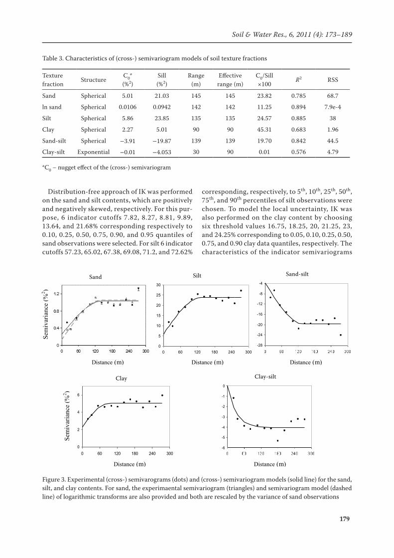
Spatial correlation

The sample (cross-) semivariograms for sand, silt, and clay percentages were calculated and then fit-ted by the weighted least squares models. To check geometric anisotropy, directional semivariograms were calculated for four azimuths 0°, 45°, 90° and

135° with 22.5° angle tolerance. The results (not shown) did not show signs of anisotropy; hence, omni-directional (cross-) semivariograms shown in Figure 3 were only considered for further analy-sis. For sand, the semivariogram of logarithmic transforms was also calculated and is presented in Figure 3; it is less erratic than the semivariogram of the raw data. In Table 3, the characteristics of (cross-) semivariogram models for soil texture frac-tion are presented. As seen, most semivariograms include a nugget effect comprising short-range variability (spatial variation occurring at distances shorter than the smallest sampling distance) and the overall measurement error. The best fitted model to the experimental (cross-) semivariogram of the soil texture fractions in terms of the highest R2 and lowest RSS coefficients functionally of GS+ (Ro-bertson 2000) is generally spherical. The degree of spatial correlation is evaluated using the ratio of nugget variance (C0) to the whole variance (Sill, Cambardella et al. 1994); the lower is the index C0/Sill, the stronger is the spatial correlation. Ac-cordingly, sand and silt having a C0/Sill < 25% are strongly spatially correlated and clay has a moder-ate spatial correlation (25% < C0/Sill < 75%). The latter is comparable with the result obtained in a study by Gallichand and Marcotte (1993) in which clay content showed a C0/Sill of 43%. They suggest, however, a different semivariogram model and correlation distance. Since clay content does not show any strong spatial correlation, silt content having a moderate correlation with clay, is used as a secondary variable to improve possibly the estimation results. As seen in Figure 3 and Table 3, using auxiliary variable even for sand and silt con-tents with a relatively strong spatial dependency improves the spatial correlation results.

Table 2. Pearson correlation coefficient (r) among soil texture fractions

Texture fraction Sand Silt Clay

Sand 1 –0.88* –0.13ns

Silt –0.88* 1 –0.36*

Clay –0.13ns –0.36* 1

*significant correlation at a significance level of P ≤ 0.05; nsnot significant

Figure 2. Histograms of sand (a) silt (b) and clay (c) contents

(a)

(b)

(c)

(a)

(b)

(c)

(a)

(b)

(c)

(a) (b) (c)

Freq

uenc

y

Sand (%) Silt (%) Clay (%)

179

Soil & Water Res., 6, 2011 (4): 173–189

Distribution-free approach of IK was performed on the sand and silt contents, which are positively and negatively skewed, respectively. For this pur-pose, 6 indicator cutoffs 7.82, 8.27, 8.81, 9.89, 13.64, and 21.68% corresponding respectively to 0.10, 0.25, 0.50, 0.75, 0.90, and 0.95 quantiles of sand observations were selected. For silt 6 indicator cutoffs 57.23, 65.02, 67.38, 69.08, 71.2, and 72.62%

corresponding, respectively, to 5th, 10th, 25th, 50th, 75th, and 90th percentiles of silt observations were chosen. To model the local uncertainty, IK was also performed on the clay content by choosing six threshold values 16.75, 18.25, 20, 21.25, 23, and 24.25% corresponding to 0.05, 0.10, 0.25, 0.50, 0.75, and 0.90 clay data quantiles, respectively. The characteristics of the indicator semivariograms

Table 3. Characteristics of (cross-) semivariogram models of soil texture fractions

Texture fraction

StructureC0*(%2)

Sill(%2)

Range(m)

Effective range (m)

C0/Sill ×100

R2 RSS

Sand Spherical 5.01 21.03 145 145 23.82 0.785 68.7

ln sand Spherical 0.0106 0.0942 142 142 11.25 0.894 7.9e-4

Silt Spherical 5.86 23.85 135 135 24.57 0.885 38

Clay Spherical 2.27 5.01 90 90 45.31 0.683 1.96

Sand-silt Spherical –3.91 –19.87 139 139 19.70 0.842 44.5

Clay-silt Exponential –0.01 –4.053 30 90 0.01 0.576 4.79

*C0 – nugget effect of the (cross-) semivariogram

Figure 3. Experimental (cross-) semivarograms (dots) and (cross-) semivariogram models (solid line) for the sand, silt, and clay contents. For sand, the experimaental semivariogram (triangles) and semivariogram model (dashed line) of logarithmic transforms are also provided and both are rescaled by the variance of sand observations

Distance (m)

Sem

ivar

ianc

e (%

2 )

Distance (m)

Clay Sand-silt

Silt Sand

Clay-silt

-28

-24

-20

-16

-12

-8

-4

-6

-5

-4

-3

-2

-1

0

0

0.4

0.8

1.2

0 60 120 180 240 3000

5

10

15

20

25

30

0 60 120 180 240 300

0

2

4

6

0 60 120 180 240 300

Distance (m)

Sem

ivar

ianc

e (%

2 )

Distance (m)

Clay Sand-silt

Silt Sand

Clay-silt

-28

-24

-20

-16

-12

-8

-4

-6

-5

-4

-3

-2

-1

0

0

0.4

0.8

1.2

0 60 120 180 240 3000

5

10

15

20

25

30

0 60 120 180 240 300

0

2

4

6

0 60 120 180 240 300

Distance (m)

Sem

ivar

ianc

e (%

2 )

Distance (m)

Clay Sand-silt

Silt Sand

Clay-silt

-28

-24

-20

-16

-12

-8

-4

-6

-5

-4

-3

-2

-1

0

0

0.4

0.8

1.2

0 60 120 180 240 3000

5

10

15

20

25

30

0 60 120 180 240 300

0

2

4

6

0 60 120 180 240 300

Distance (m)

Sem

ivar

ianc

e (%

2 )

Distance (m)

Clay Sand-silt

Silt Sand

Clay-silt

-28

-24

-20

-16

-12

-8

-4

-6

-5

-4

-3

-2

-1

0

0

0.4

0.8

1.2

0 60 120 180 240 3000

5

10

15

20

25

30

0 60 120 180 240 300

0

2

4

6

0 60 120 180 240 300

Distance (m)

Sem

ivar

ianc

e (%

2 )

Distance (m)

Clay Sand-silt

Silt Sand

Clay-silt

-28

-24

-20

-16

-12

-8

-4

-6

-5

-4

-3

-2

-1

0

0

0.4

0.8

1.2

0 60 120 180 240 3000

5

10

15

20

25

30

0 60 120 180 240 300

0

2

4

6

0 60 120 180 240 300

Distance (m)

Sem

ivar

ianc

e (%

2 )

Distance (m)

Clay Sand-silt

Silt Sand

Clay-silt

-28

-24

-20

-16

-12

-8

-4

-6

-5

-4

-3

-2

-1

0

0

0.4

0.8

1.2

0 60 120 180 240 3000

5

10

15

20

25

30

0 60 120 180 240 300

0

2

4

6

0 60 120 180 240 300

Distance (m)

Sem

ivar

ianc

e (%

2 )

Distance (m)

Clay Sand-silt

Silt Sand

Clay-silt

-28

-24

-20

-16

-12

-8

-4

-6

-5

-4

-3

-2

-1

0

0

0.4

0.8

1.2

0 60 120 180 240 3000

5

10

15

20

25

30

0 60 120 180 240 300

0

2

4

6

0 60 120 180 240 300

Distance (m)

Sem

ivar

ianc

e (%

2 )

Distance (m)

Clay Sand-silt

Silt Sand

Clay-silt

-28

-24

-20

-16

-12

-8

-4

-6

-5

-4

-3

-2

-1

0

0

0.4

0.8

1.2

0 60 120 180 240 3000

5

10

15

20

25

30

0 60 120 180 240 300

0

2

4

6

0 60 120 180 240 300

Distance (m)

Sem

ivar

ianc

e (%

2 )

Distance (m)

Clay Sand-silt

Silt Sand

Clay-silt

-28

-24

-20

-16

-12

-8

-4

-6

-5

-4

-3

-2

-1

0

0

0.4

0.8

1.2

0 60 120 180 240 3000

5

10

15

20

25

30

0 60 120 180 240 300

0

2

4

6

0 60 120 180 240 300

Distance (m)

Sem

ivar

ianc

e (%

2 )

Distance (m)

Clay Sand-silt

Silt Sand

Clay-silt

-28

-24

-20

-16

-12

-8

-4

-6

-5

-4

-3

-2

-1

0

0

0.4

0.8

1.2

0 60 120 180 240 3000

5

10

15

20

25

30

0 60 120 180 240 300

0

2

4

6

0 60 120 180 240 300

Silt Sand-silt

Clay Clay-silt

Sand

Distance (m)

Sem

ivar

ianc

e (%

2 )

Distance (m)

Clay Sand-silt

Silt Sand

Clay-silt

-28

-24

-20

-16

-12

-8

-4

-6

-5

-4

-3

-2

-1

0

0

0.4

0.8

1.2

0 60 120 180 240 3000

5

10

15

20

25

30

0 60 120 180 240 300

0

2

4

6

0 60 120 180 240 300

180

Soil & Water Res., 6, 2011 (4): 173–189

are given in Table 4. The models are fitted using a combination of fitting by eye and the weighted least squares. Most of the indicator semivariograms show a moderate spatial correlation within the classes for the texture fractions.

Estimation and uncertainty assessment

Cross-validation results of sand, silt, and clay contents estimation using OK, LOK, COK, and full IK are presented in Table 5. The results indicated that IK is the most accurate method (RMSE = 3.12%) for estimating the sand content whereas the highest error was obtained with LOK (RMSE = 3.24%). The scatterplots of the sand observations

versus the estimates from OK, LOK, and full IK are displayed in Figure 4. With all methods, the estimated mean value is similar to the actual mean value (without bias), and standard deviation (SD) of the estimated values is smaller than the sam-pled one (smoothness). IK, however, achieved the highest correlation coefficient between the sand observations and estimates. Surprisingly, IK smoothed out the sand estimates at the most, which may be due to an insufficient indicators selected. The smoothing effect was the least for COK, yet it gave a correlation coefficient quite similar to IK. This highlights the usefulness of the secondary variable (i.e. silt content) for improving the sand estimation results. The most accurate method for estimating the silt content appeared

Table 4. Indicator semivariogram characteristics of sand, silt, and clay contents

Texture fraction

Quantile StructurC0

(%2)Sill(%2)

Range (m)

Effectiverange (m)

C0/Sill × 100

R2 RSS

Sand

0.1Sph.Exp.

0.040.001

0.0980.097

18040

180120

40.821.03

0.6820.761

1.92e-31.45e-3

0.25Sph.Exp.

0.060.041

0.1930.197

8536

85108

31.0920.81

0.8320.89

1.94e-31.29e-3

0.50Sph.Exp.

0.180.128

0.2560.257

13031

13093

70.3149.81

0.6730.538

1.96e-32.97e-3

0.75Sph.Exp.

0.0520.027

0.1920.195

10539

105117

27.0813.85

0.9080.893

1.37e-31.61e-3

0.90 Sph. 0.026 0.095 160 160 27.37 0.881 6.7e-4

0.95 Sph. 0.011 0.036 90 90 30.56 0.687 1.61e-4

Silt

0.05 Sph. 0.015 0.043 130 130 34.88 0.702 2.97e-4

0.1 Sph. 0.028 0.096 160 160 29.17 0.898 5.85e-4

0.25 Sph. 0.099 0.20 140 140 49.5 0.496 5.03e-3

0.50 Sph. 0.17 0.26 160 160 65.38 0.780 1.96e-3

0.75Sph.Exp.

0.0010.001

0.1900.193

7028.3

7085

0.530.52

0.9150.873

1.35e-32.20e-3

0.90 Sph. 0.027 0.079 95 95 34.18 0.802 3.92e-4

Clay

0.05 Sph. 0.0001 0.0394 72 72 0.25 0.721 7.8e-4

0.1 Exp. 0.0354 0.0978 42 126 36.20 0.764 7.4e-4

0.25 Exp. 0.0001 0.1982 26 78 0.05 0.824 4e-3

0.50 Exp. 0.0001 0.2522 22 66 0.04 0.846 3e-3

0.75 Exp. 0.0112 0.1684 17 51 6.65 0.732 1.2e-3

0.90 Exp. 0.0001 0.0826 15 45 0.12 0.516 6e-4

181

Soil & Water Res., 6, 2011 (4): 173–189

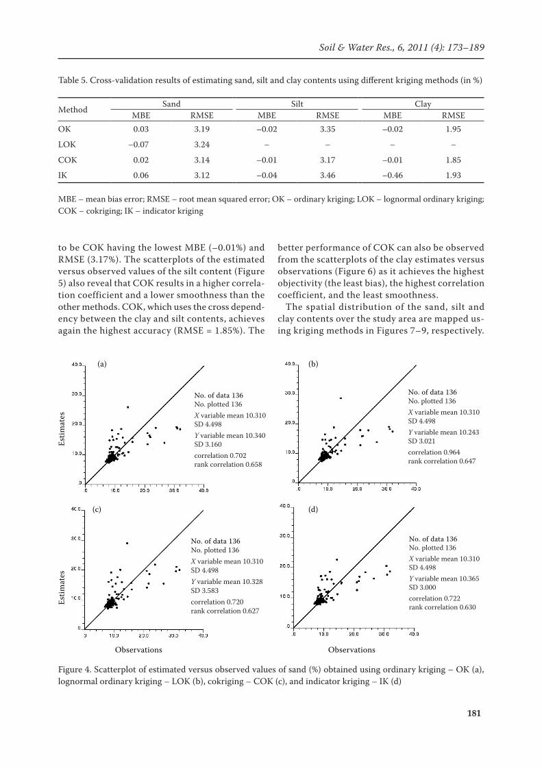
to be COK having the lowest MBE (–0.01%) and RMSE (3.17%). The scatterplots of the estimated versus observed values of the silt content (Figure 5) also reveal that COK results in a higher correla-tion coefficient and a lower smoothness than the other methods. COK, which uses the cross depend-ency between the clay and silt contents, achieves again the highest accuracy (RMSE = 1.85%). The

better performance of COK can also be observed from the scatterplots of the clay estimates versus observations (Figure 6) as it achieves the highest objectivity (the least bias), the highest correlation coefficient, and the least smoothness.

The spatial distribution of the sand, silt and clay contents over the study area are mapped us-ing kriging methods in Figures 7–9, respectively.

Table 5. Cross-validation results of estimating sand, silt and clay contents using different kriging methods (in %)

MethodSand Silt Clay

MBE RMSE MBE RMSE MBE RMSEOK 0.03 3.19 –0.02 3.35 –0.02 1.95

LOK –0.07 3.24 – – – –

COK 0.02 3.14 –0.01 3.17 –0.01 1.85

IK 0.06 3.12 –0.04 3.46 –0.46 1.93

MBE – mean bias error; RMSE – root mean squared error; OK – ordinary kriging; LOK – lognormal ordinary kriging; COK – cokriging; IK – indicator kriging

Figure 4. Scatterplot of estimated versus observed values of sand (%) obtained using ordinary kriging – OK (a), lognormal ordinary kriging – LOK (b), cokriging – COK (c), and indicator kriging – IK (d)

Estim

ates

Estim

ates

Observations Observations

No. of data 136No. plotted 136X variable mean 10.310SD 4.498Y variable mean 10.340SD 3.160correlation 0.702rank correlation 0.658

(a)


(b)


(c)


(d)

182

Soil & Water Res., 6, 2011 (4): 173–189

Figure 5. Scatterplot of estimated versus observed va-lues of silt (%) obtained using ordinary kriging – OK (a), cokriging – COK (b), and indicator kriging – IK (c)

Observations

Estim

ates

Observations

Estim

ates


(a) (b)


(c)


Figure 6. Scatterplot of estimated versus observed values of clay (%) using ordinary kriging – OK (a), cokriging – COK (b), and indicator kriging – IK (c)

Observations

Observations

Estim

ates

Estim

ates

(a)


(b)


(c)


183

Soil & Water Res., 6, 2011 (4): 173–189

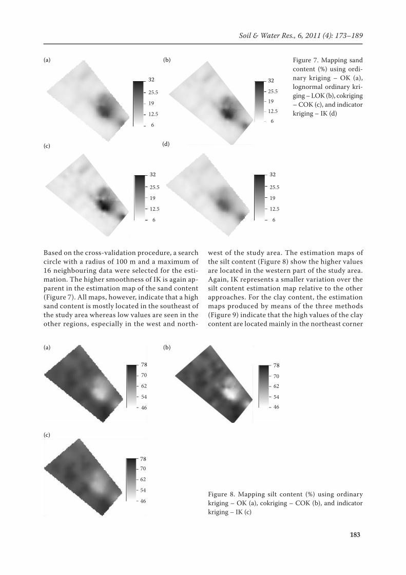
Based on the cross-validation procedure, a search circle with a radius of 100 m and a maximum of 16 neighbouring data were selected for the esti-mation. The higher smoothness of IK is again ap-parent in the estimation map of the sand content (Figure 7). All maps, however, indicate that a high sand content is mostly located in the southeast of the study area whereas low values are seen in the other regions, especially in the west and north-

west of the study area. The estimation maps of the silt content (Figure 8) show the higher values are located in the western part of the study area. Again, IK represents a smaller variation over the silt content estimation map relative to the other approaches. For the clay content, the estimation maps produced by means of the three methods (Figure 9) indicate that the high values of the clay content are located mainly in the northeast corner

Figure 7. Mapping sand content (%) using ordi-nary kriging – OK (a), lognormal ordinary kri-ging – LOK (b), cokriging – COK (c), and indicator kriging – IK (d)

Figure 8. Mapping silt content (%) using ordinary kriging – OK (a), cokriging – COK (b), and indicator kriging – IK (c)

(a) (b)

(c)

78

70

62

54

46

78

70

62

54

46

7870

62

54

46

(b)

(d)

(a)

(c)

(a)

(c)

32

25.5

19

12.5

6

32

25.5

19

12.5

6

32

25.5

19

12.5

6

32

25.5

19

12.5

6

(d)

(b)

184

Soil & Water Res., 6, 2011 (4): 173–189

while the low valued-areas are mostly located in the south and southwest corners of the study area.

The estimation variance produced through OK, LOK, and COK, and IK-conditional variance of the sand estimates are mapped in Figure 10. The estimation error variance (uncertainty) provided by OK, LOK, and COK is, as expected, smaller at the sampling sites and nearby locations and it becomes higher as the distance between the observations is getting larger (south part of the study area) and where no data is available (the east and southeast parts of the study area). The conditional variances

produced by IK show in contrast some relation with the sand data values in addition to the data configuration. Figure 10(d) indicates that the un-certainty of the sand estimate is smaller where the data are consistently small or intermediate (most parts of the western and northern area). The lo-cal uncertainty is larger in the high-valued areas in the south eastern area where high values are isolated, i.e. a few high values are surrounded by small values of sand. To evaluate the uncertainty model provided by OK and IK, the scatterplot of the estimation errors versus standard deviations is

Figure 10. OK-variance (a) LOK--variance (b) COK-variance (c) and IK-conditional variance (d) of sand estimates (%)

Figure 9. Mapping clay content (%) using ordinary kriging – OK (a), cokriging – COK (b), and indicator kriging – IK (c)

(a) (b)

(c)

2724

21

18

15

27

24

21

18

15

2724

21

18

15

(a) (b)

(c) (d)

(a) (b)

(c) (d)

8060

40

20

0

8060

40

20

0

8060

40

20

0

8060

40

20

0

185

Soil & Water Res., 6, 2011 (4): 173–189

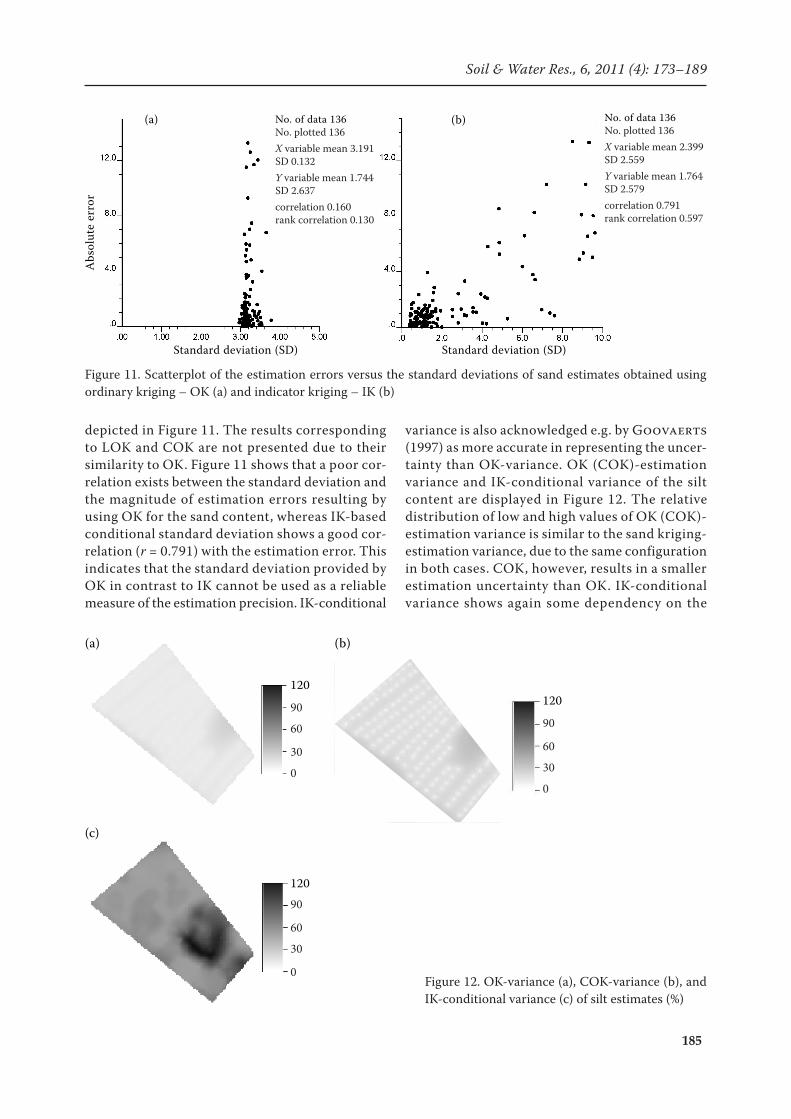
depicted in Figure 11. The results corresponding to LOK and COK are not presented due to their similarity to OK. Figure 11 shows that a poor cor-relation exists between the standard deviation and the magnitude of estimation errors resulting by using OK for the sand content, whereas IK-based conditional standard deviation shows a good cor-relation (r = 0.791) with the estimation error. This indicates that the standard deviation provided by OK in contrast to IK cannot be used as a reliable measure of the estimation precision. IK-conditional

variance is also acknowledged e.g. by Goovaerts (1997) as more accurate in representing the uncer-tainty than OK-variance. OK (COK)-estimation variance and IK-conditional variance of the silt content are displayed in Figure 12. The relative distribution of low and high values of OK (COK)-estimation variance is similar to the sand kriging-estimation variance, due to the same configuration in both cases. COK, however, results in a smaller estimation uncertainty than OK. IK-conditional variance shows again some dependency on the

Figure 11. Scatterplot of the estimation errors versus the standard deviations of sand estimates obtained using ordinary kriging – OK (a) and indicator kriging – IK (b)

Standard deviation (SD)

Abs

olut

e er

ror


(a) No. of data 136No. plotted 136X variable mean 3.191SD 0.132Y variable mean 1.744SD 2.637correlation 0.160rank correlation 0.130

(b) No. of data 136No. plotted 136X variable mean 2.399SD 2.559Y variable mean 1.764SD 2.579correlation 0.791rank correlation 0.597

Figure 12. OK-variance (a), COK-variance (b), and IK-conditional variance (c) of silt estimates (%)

(c)

(a) (b)

(c)

120

90

60

30

0

120

90

60

30

0

120

90

60

30

0

186

Soil & Water Res., 6, 2011 (4): 173–189

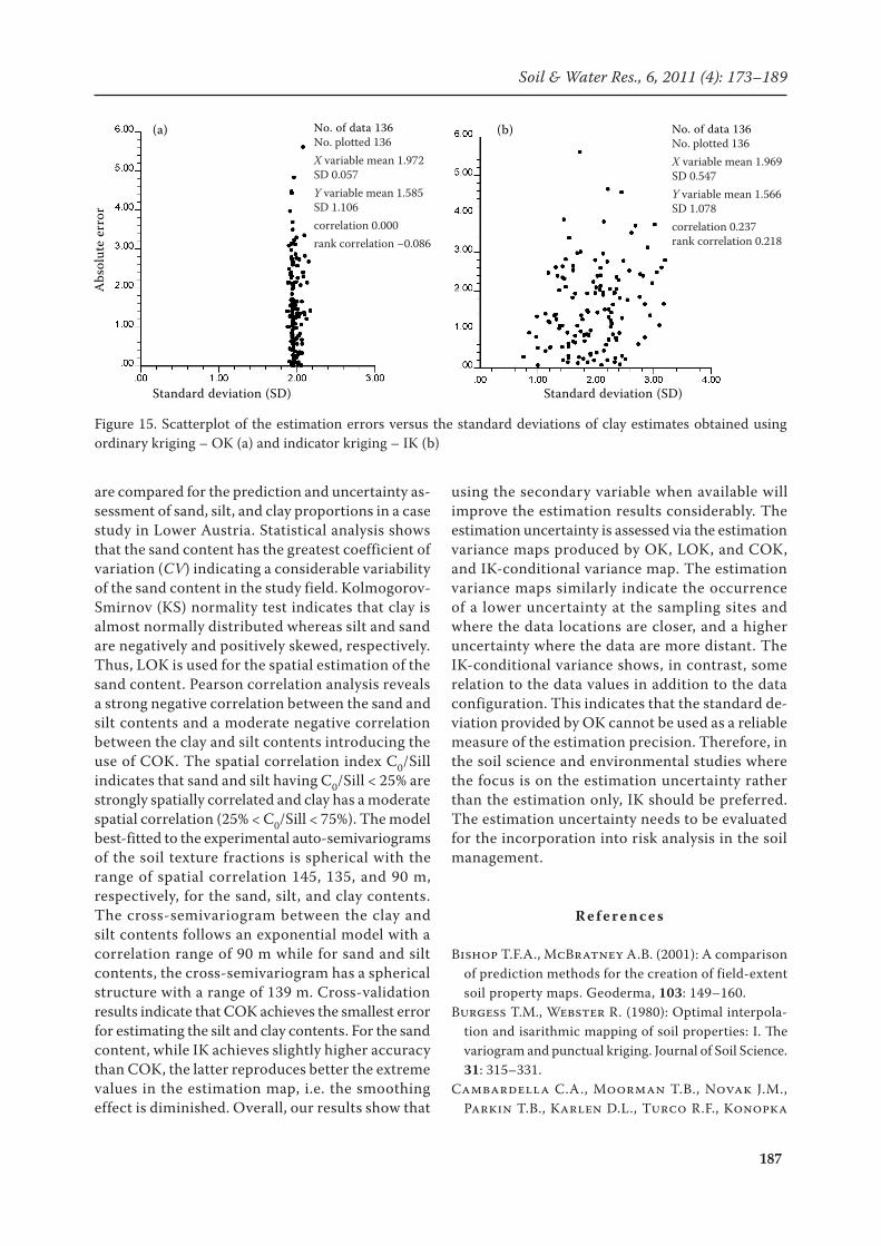
sample data. As seen also in Figure 13, a good correlation (r = 0.607) exists between the absolute error and standard deviation obtained through IK whereas the correlation for OK is quite poor. This indicates that IK-conditional standard deviation can be used as a better representative measure of the silt estimation precision. In Figure 14, the OK (COK)-estimation variance and conditional vari-ance for the clay content estimates are presented. Again, the OK (COK)-variance maps indicate that there is a low uncertainty where the data locations are closer and a high uncertainty where they are more distant. In no similar way, IK-conditional variance map indicates that the areas of a high

uncertainty (wider ccdfs) are located mostly in the north and west of the study area where the transition from the high to the low values occurs within short distances. There is a low correlation between the absolute error and standard deviation obtained through IK and no correlation for those obtained by OK for the clay content (Figure 15).

SUMMARY AND CONCLUSIONS

Geostatistical estimation methods including ordinary kriging (OK), lognormal ordinary kriging (LOK), cokriging (COK), and indicator kriging (IK)

Figure 14. OK-variance (a), COK-variance (b), and IK-conditional variance (c) of clay estimates

Figure 13. Scatterplot of the estimation errors versus the standard deviations of silt estimates obtained using or-dinary kriging – OK (a) and indicator kriging – IK (b)


Abs

olut

e er

ror



(a) (b) No. of data 136No. plotted 136X variable mean 3.165SD 2.308Y variable mean 2.307SD 2.576correlation 0.607rank correlation 0.406

(b)

(c)

(a) (b)

(c)

21

14

7

0

21

14

7

0

21

14

7

0

187

Soil & Water Res., 6, 2011 (4): 173–189

are compared for the prediction and uncertainty as-sessment of sand, silt, and clay proportions in a case study in Lower Austria. Statistical analysis shows that the sand content has the greatest coefficient of variation (CV) indicating a considerable variability of the sand content in the study field. Kolmogorov-Smirnov (KS) normality test indicates that clay is almost normally distributed whereas silt and sand are negatively and positively skewed, respectively. Thus, LOK is used for the spatial estimation of the sand content. Pearson correlation analysis reveals a strong negative correlation between the sand and silt contents and a moderate negative correlation between the clay and silt contents introducing the use of COK. The spatial correlation index C0/Sill indicates that sand and silt having C0/Sill < 25% are strongly spatially correlated and clay has a moderate spatial correlation (25% < C0/Sill < 75%). The model best-fitted to the experimental auto-semivariograms of the soil texture fractions is spherical with the range of spatial correlation 145, 135, and 90 m, respectively, for the sand, silt, and clay contents. The cross-semivariogram between the clay and silt contents follows an exponential model with a correlation range of 90 m while for sand and silt contents, the cross-semivariogram has a spherical structure with a range of 139 m. Cross-validation results indicate that COK achieves the smallest error for estimating the silt and clay contents. For the sand content, while IK achieves slightly higher accuracy than COK, the latter reproduces better the extreme values in the estimation map, i.e. the smoothing effect is diminished. Overall, our results show that

using the secondary variable when available will improve the estimation results considerably. The estimation uncertainty is assessed via the estimation variance maps produced by OK, LOK, and COK, and IK-conditional variance map. The estimation variance maps similarly indicate the occurrence of a lower uncertainty at the sampling sites and where the data locations are closer, and a higher uncertainty where the data are more distant. The IK-conditional variance shows, in contrast, some relation to the data values in addition to the data configuration. This indicates that the standard de-viation provided by OK cannot be used as a reliable measure of the estimation precision. Therefore, in the soil science and environmental studies where the focus is on the estimation uncertainty rather than the estimation only, IK should be preferred. The estimation uncertainty needs to be evaluated for the incorporation into risk analysis in the soil management.

R e f e r e n c e s

Bishop T.F.A., McBratney A.B. (2001): A comparison of prediction methods for the creation of field-extent soil property maps. Geoderma, 103: 149–160.

Burgess T.M., Webster R. (1980): Optimal interpola-tion and isarithmic mapping of soil properties: I. The variogram and punctual kriging. Journal of Soil Science. 31: 315–331.

Cambardella C.A., Moorman T.B., Novak J.M., Parkin T.B., Karlen D.L., Turco R.F., Konopka

Figure 15. Scatterplot of the estimation errors versus the standard deviations of clay estimates obtained using ordinary kriging – OK (a) and indicator kriging – IK (b)

Standard deviation (SD) Standard deviation (SD)

Abs

olut

e er

ror

No. of data 136No. plotted 136X variable mean 1.972SD 0.057Y variable mean 1.585SD 1.106correlation 0.000rank correlation −0.086

(a) (b) No. of data 136No. plotted 136X variable mean 1.969SD 0.547Y variable mean 1.566SD 1.078correlation 0.237rank correlation 0.218

188

Soil & Water Res., 6, 2011 (4): 173–189

A.E. (1994): Field-scale variability of soil properties in central Iowa soils. Soil Science Society of American Journal, 58: 1501–1511.

Delbari M. (2007): Estimation and stochastic simula-tion of soil properties for case studies in Lower Austria and Sistan plain, southeast of Iran. [PhD. Thesis.] University of Natural Resources and Applied Life Sci-ences, Vienna.

Deutsch C.V., Journel A.G. (1998): GSLIB: Geostatis-tical Software Library and User’s Guide. 2nd Ed. Oxford University Press, New York.

Ersahin S., Brohi A.R. (2006): Spatial variation of soil water content in topsoil and subsoil of a Typic Ustif-luvent. Agricultural Water Management, 83: 79–86.

Ersahin S. (2003): Comparing ordinary kriging and cokriging to estimate infiltration rate. Soil Science Society of American Journal, 67: 1848–1855.

Gallichand J., Marcotte D. (1993): Mapping clay content for subsurface drainage in the Nile Delta. Geoderma, 58: 165–179.

Gaston L.A., Locke M.A., Zablotowicz R.M., Reddy K.N. (2001): Spatial variability of soil properties and weed populations in the Mississippi delta. Soil Science Society of American Journal, 65: 449–459.

Gonzalez O.J., Zak D.R. (1994): Geostatistical analysis of soil properties in a secondary tropical dry forest, St. Lucia, West Indies. Plant and Soil, 163: 45–54.

Goovaerts P. (1997): Geostatistics for Natural Resourc-es Evaluation. Oxford University Press, New York.

Goovaerts P. (1998): Geostatistical tools for charac-terizing the spatial variability of microbiological and physico-chemical soil properties. Biology and Fertility of Soils, 27: 315–334.

Goovaerts P. (1999): Geostatistics in soil science: state-of-the-art and perspectives. Geoderma, 89: 1–45.

Goovaerts P., Webster R., Dubois J.-P. (1997): As-sessing the risk of soil contamination in the Swiss Jura using indicator geostatistics. Environmental and Ecological Statistics, 4: 31–48.

Gotway C.A. Hartford A.H. (1996): Geostatistical methods for incorporating auxiliary information in the prediction of spatial variables. Journal of Agricultural, Biological and Environmental Statistics, 1: 17–39.

Gupta S.C., Larson W.E. (1979): Estimating soil water retention characteristics from particle size distribu-tion, organic matter content, and bulk density. Water Resources Research, 15: 1633–1635.

Isaaks E.H., Srivastava R.M. (1989): An Introduction to Applied Geostatistics. Oxford University Press, New York.

Journel A.G. (1983): Non-parametric estimation of spa-tial distributions. Mathematical Geology, 15: 445–468.

Journel A.G., Huijbregts C.J. (1978): Mining Geosta-tistics. Academic Press, New York.

Juang K.W., Lee D.Y. (1998): A comparison of three kriging methods using auxiliary variables in heavy-metal contaminated soils. Journal of Environmental Quality, 27: 355–363.

Kerry R., Oliver M. (2003): Variograms of ancillary data to aid sampling for soil surveys. Precision Agri-culture, 4: 261–278.

Lloyd C.D., Atkinson P.M. (1999): Designing optimal sampling configurations with ordinary and indicator kriging. In: 4th Int. Conf. GeoComputation 99. July 25–28, Fredericksburg.

López-Granados F., Jurado-Expósito M., Aten-ciano S., García-Ferrer A., Sánchez de la Orden M., García-Torres L. (2002): Spatial variability of agricultural soil parameters in southern Spain. Plant Soil, 246: 97–105.

López-Granados F., Jurado-Expósito M., Pena-Barragan J.M., García-Torres L. (2005): Using geostatistical and remote sensing approaches for map-ping soil properties. European Journal of Agronomy, 23: 279–289.

Mohammadi J., Van Meirvenne M., Goovaerts P. (1997): Mapping cadmium concentration and the risk of exceeding a local sanitation threshold using indica-tor geostatistics. In: Soares A., Gómez-Hernández J., Froidevaux R. (eds): GeoENV I – Geostatistics for Environmental Applications. Kluwer, Dordrecht, 327–337.

Morgan R.P.C., Quinton J.N., Smith R.E., Govers G., Poesen J.W.A., Auerswald K., Chisci G., Torri D., Styczen M.E. (1998): The European Soil Ero-sion Model (EUROSEM): A dynamic approach for predicting sediment transport from fields and small catchments. Earth Surface Processes and Landforms, 23: 527–544.

Nogueira F., Couto E.G., Bernardi C.J. (2002): Geo-statistics as a tool to improve sampling and statistical analysis in wetlands: A case study on dynamics of organ-ic matter distribution in the Pantanal of Mato Grosso, Brazil. Brazilian Journal of Biology, 62: 861–870.

Odeh I.O.A., Todd A.J., Triantafilis J. (2003): Spatial prediction of soil particle-size fractions as composi-tional data. Soil Science, 168: 501–515.

Patriarche D., Castro M.C., Goovaerts P. (2005): Estimating regional hydraulic conductivity fields—A comparative study of geostatistical methods. Math-ematical Geology, 37: 587–613.

Rawls W.J., Brakensiek D.L., Saxton K.E. (1982): Estimation of soil water properties. Transactions of ASAE, 25: 1316–1320.

189

Soil & Water Res., 6, 2011 (4): 173–189

Robertson G.P. (2000): GS+: Geostatistics for the En-vironment Sciences. GS+ User’s Guide Version 5. Gamma Design Software, Plainwell.

Saito H., Goovaerts P. (2000): Geostatistical inter-polation of positively skewed and censored data in a dioxin-contaminated site. Environmental Science and Technology, 34: 4228–4235.

Trangmar B.B., Yost R.S., Uehara G. (1985): Applica-tion of geostatistics to spatial studies of soil properties. Advances in Agronomy, 38: 45–93.

Triantafilis J., Odeh I.O.A., McBratney A.B. (2001): Five geostatistical models to predict soil salinity from electromagnetic induction data across irrigated cot-ton. Soil Science Society of American Journal, 65: 869–878.

Vaughan P.J., Lesch S.M., Corwin D.L., Cone D.G. (1995): Water content effect on soil salinity prediction: A geostatistical study using cokriging. Soil Science Society of American Journal, 59: 1146–1156.

Voltz M., Lagacherie P., Louchart X. (1997): Pre-dicting soil properties over a region using sample information from a mapped reference area. European Journal of Soil Science, 48: 19–30.

Yates S.R., Warrick A.W. (1987): Estimating soil wa-ter content using cokriging. Soil Science Society of American Journal, 51: 23–30.

Zhang R., Myers D.E., Warrick A.W. (1992): Esti-mation of spatial distribution of soil chemicals us-ing pseudo-cross-variograms. Soil Science Society of American Journal, 56: 1444–1452.

Zhang R., Shouse P., Yates S. (1997): Use of pseudo-crossvariograms and cokriging to improve estimates of soil solute concentrations. Soil Science Society of American Journal, 61: 1342–1347.

Zötl J.G. (1997): The spa Deutsch-Altenburg and the hydrogeology of the Vienna basin (Austria). Environ-mental Geology, 29: 176–187.

Received for publication February 26, 2010Accepted after corrections March 10, 2011

Corresponding author:

Dr. Masoomeh Delbari, University of Zabol, Faculty of Agriculture, Department of Water Engineering, Zabol, Irane-mail: [email protected]

geostatistical analysis of soil texture fractions on the ... · pdf file175 soil & water...

Documents